ERASMUS UNIVERSITY ROTTERDAM

Solving the Locomotive AssignmentProblem for a European rail-passenger

and rail-cargo company

Master’s ThesisEconometrics and Management Science

Operations Research and Quantitative Logistics

Ivan Olthuis (359299)

November 4, 2015

Erasmus University Rotterdam Ab Ovo InternationalErasmus School of Economics Business Unit AdvancedSupervisor: Planning and SchedulingDr. Wilco van den Heuvel Supervisors:Co-reader: Drs. Dieter VeldhuisDr. Twan Dollevoet Drs. Peter Koot

Abstract

This thesis considers a large real-life application of the Locomotive Assignment

Problem. Due to the large size of the problem instance, many of the existing

solution methods are unlikely to find a good quality solution within reason-

able computation time. In this thesis, we define two different multi-commodity

flow formulations, where the commodities correspond to locomotive types and

consists, respectively. The formulation based on locomotive types provides the

optimal solution, while the consist based formulation is unlikely to reach opti-

mality. Next to the two formulations, two different heuristics are investigated.

The first heuristic is a relax-and-fix heuristic, which aims to solve the locomotive

based formulation iteratively by decomposing the set of arcs into subsets based

on starting time. The second heuristic is a greedy heuristic extended with a local

search heuristic. This approach schedules every activity such that the additional

cost for this activity is minimized. Afterwards, the solution is improved by in-

vestigating neighbouring solutions. Especially the relax-and-fix heuristic is able

to provide good quality results within reasonable computation time for the real

size dataset.

Keywords: Locomotive Assignment Problem; Multi-commodity flow formulations;

Relax-and-fix heuristic; Greedy heuristic

i

Table of contents

1 Introduction 1

2 Problem Description 3

3 Literature Review 73.1 Homogeneous locomotives and single-locomotive consists . . . . . . . . 73.2 Heterogeneous set of locomotives and single-locomotive consists . . . . 73.3 Heterogeneous set of locomotives and multi-locomotive consists . . . . 93.4 General findings . . . . . . . . . . . . . . . . . . . . . . . . . . . . . . 15

4 Data Description 16

5 Mathematical Formulation 205.1 Defining the time-space network . . . . . . . . . . . . . . . . . . . . . 205.2 Notation . . . . . . . . . . . . . . . . . . . . . . . . . . . . . . . . . . . 265.3 Multi-commodity flow problem with side constraints . . . . . . . . . . 28

6 Methodology 316.1 Locomotive based flow formulation . . . . . . . . . . . . . . . . . . . . 31

6.1.1 Generating light traveling arcs . . . . . . . . . . . . . . . . . . 316.2 Consist based flow formulation . . . . . . . . . . . . . . . . . . . . . . 336.3 Relax-and-Fix heuristic . . . . . . . . . . . . . . . . . . . . . . . . . . 356.4 Greedy heuristic . . . . . . . . . . . . . . . . . . . . . . . . . . . . . . 38

6.4.1 Sequencing activities . . . . . . . . . . . . . . . . . . . . . . . . 396.4.2 Assigning activities to loc lines . . . . . . . . . . . . . . . . . . 406.4.3 Local search . . . . . . . . . . . . . . . . . . . . . . . . . . . . . 42

7 Computational Results 457.1 Generating different problem instances . . . . . . . . . . . . . . . . . . 457.2 Results for the small problem instances . . . . . . . . . . . . . . . . . 467.3 Results for the medium size problem instances . . . . . . . . . . . . . 527.4 Results for the real-life dataset . . . . . . . . . . . . . . . . . . . . . . 577.5 Varying the turntime . . . . . . . . . . . . . . . . . . . . . . . . . . . . 63

8 Conclusion 65

9 Further Research 68

1 Introduction

In current society, transport is an important factor with the ever increasing level

of globalization. Especially in Europe, transport by rail is a convenient mode of

transportation since the distances between countries are relatively small, although

advanced operational models are required in order to compete with other means of

transportation. When thinking about rail transport, one can distinguish between two

different types of transport: passenger transport and freight transport. In this study,

both means of transportation will be taken into account. It is important to distinguish

between passenger and freight transport, because there are large differences in weight

of the trains and the timetables of the two modes of transportation are incomparable.

The use of optimization models in the field of rail transport has increased immensely

during the last decade, which is mainly due to the fierce competition between different

railroad companies, see Piu (2011). Furthermore, the increased speed of computers

enables the use of optimization models, since the optimization models are usually

very complex for these kinds of problems. As the use of optimization models has

become popular recently, this study deals with a subject which is of current interest.

This study focuses on a specific part in the process of optimizing the planning for

rail transport, namely assigning a set of locomotives to a network of trains. When

assigning these locomotives, the main goal will be to minimize costs, while taking

several side constraints into account. A schedule for all trains needs to be obtained

first, before the set of locomotives can be assigned to this network of trains. Obtain-

ing this schedule will not be part of this study. According to Ahuja et al. (2002),

locomotive scheduling problems are amongst the most important problems in railroad

scheduling. However, few papers propose methods which are able to cope with large

real-world instances. In real-life instances there are often large numbers of locomo-

tives which need to be assigned and hence making use of optimization models can

lead to large economic savings even when the relative improvement is fairly small, see

Piu (2011). Apart from minimizing total costs, it is also important to obtain a good

schedule in general. With locomotive scheduling, a good schedule should be robust

such that possible delays or other issues have limited impact.

The problem faced in this study is a real-life scheduling problem for a large Euro-

pean rail-passenger and rail-cargo company. A weekly schedule should be obtained,

where around 4,200 activities need to be assigned to a total of 374 locomotives. Since

the size of this scheduling problem is fairly large compared to data instances in other

studies, it is important to develop methods which are able to deal with this larger

1

instance size. But most importantly, many of the locomotives have to be moved be-

tween different activities, which increases the difficulty of the problem faced. Moving

locomotives may be done at any moment during the week, which increases the num-

ber of possible solutions immensely. This additional difficulty is barely discussed in

other papers, either because the problem is such that repositioning is not required,

or a limited number of repositioning opportunities is sufficient to obtain a feasible

solution.

The remainder of this thesis is organized as follows: In Chapter 2, an extensive

problem description is provided. Chapter 3 reviews the related literature, and states

whether the proposed methods might be useful for our study. In Chapter 4, the data

which is used for this study will be discussed in more detail. Chapter 5 describes how

the network is created, and the MIP formulation which follows from this network is

discussed. Chapter 6 describes the different methods in more detail. Then, in Chapter

7 the main results are summarized and conclusions about the different methods are

drawn. Chapter 8 states the main findings of this research, and ideas for further

research are mentioned in Chapter 9.

2

2 Problem Description

The problem of assigning a set of locomotives to cover all scheduled trains while

satisfying several side constraints is known as the Locomotive Assignment Problem

(LAP in the following) in the literature, see Ahuja et al. (2002). The main goal

of the LAP is to assign locomotives to scheduled trains such that the allocation of

locomotives results in minimizing a certain objective. Kasalica et al. (2013) mention

that locomotive scheduling problems can be studied at two different levels: on the

strategic level and at the operational level. At the strategic level, the objective of

the LAP will focus on minimizing the total number of locomotives. This question is

especially interesting if a company wants to know how many locomotives they need

to purchase. On the other hand, if the number of locomotives is known beforehand,

planning at an operational level will be applied. At the operational level, the objective

of the LAP aims to minimize total costs, which are mainly caused by deadheading and

light traveling, by assigning locomotives effectively to activities, as will be explained

later in this chapter. Since the number of available locomotives is known in this

study, the main goal of the LAP will be to minimize the total costs by optimizing

the allocation of locomotives.

In this study, three different kinds of activities need to be planned:

• Assigning locomotives to passenger trains.

• Assigning locomotives to cargo trains.

• Assigning locomotives to fulfill different yard activities. We will refer to those

activities as loc orders in the following of this thesis.

It is important to make a distinction between these three different activity types,

because each of the activities has different characteristics. The main differences

between passenger transport and freight transport are the large differences in train

weights and the timetable of the trains. As one can imagine, cargo trains are heavier

than passenger trains which influences the number of locomotives that needs to be

assigned to a train. Furthermore, passenger trains are usually operational between

5 AM and 12 PM, while freight trains are also operative during night time. The

loc orders can be distinguished into two different types of activities: train related loc

orders and non-train related loc orders. Train related loc orders are always associated

to a passenger or cargo related activity, and therefore these loc orders are performed

3

by the same set of locomotives as their associated activity. Train related loc orders

are activities such as performing brake tests or repositioning an arriving train at the

yard. Non-train related activities are activities such as repositioning wagons at the

yard or performing certain maintenance activities.

Each of these activities requires a certain number of locomotives. Especially for

cargo related activities, assigning one locomotive to an activity is usually insufficient.

Therefore, it is possible to use multiple locomotives in order to provide enough power

to be able to fulfill the activity. In this case, the locomotives are restricted to be of

the same locomotive type. A combination of one locomotive or multiple locomotives

is called a consist.

For each of the activities so called possible tractions are defined. The possible

tractions denote for each activity which consists are able to perform the activity.

More formally, the possible tractions denote the set of feasible consists for each of the

activities. There are several reasons why a consist could not be able to perform an

activity. First, there are crew related arguments. Especially for the newer locomotive

types, not all employees have licences which allow them to drive on these locomotives.

If at some locations an insufficient number of employees is present, it could occur that

there are some activities which cannot be performed by certain consists. Secondly,

not all consists will provide a sufficient amount of horse power. Apart from horse

power restrictions, there are also locomotives which have a maximum speed which is

too low for some of the activities. In this case, it is also not allowed to assign a consist

containing this locomotive to these activities. Finally, there are tracks which cannot

handle electric locomotives, since the required wiring is missing. In this case, consists

containing an electric locomotive cannot be assigned to an activity. For each of the

consists the associated costs are known based on locomotive type and the number of

locomotives which are used.

Each activity has an associated starting and ending location. In general, those

locations will differ from each other, but in case of the loc orders the start and ending

location are always the same. Of course, a consist can only be assigned to a certain

activity if all of the locomotives within this consist are at the starting location at

the starting time of the activity. However, it is not expected that this is achieved

at all times by just assigning locomotives to activities. For example, a cargo train

leaving from a lumberyard needs more horsepower to pull the train compared to

arriving there. If there is only one train entering and leaving this location each day, a

shortage of locomotives will arise at this location. Since there are no other incoming

4

locomotives, it is necessary to move locomotives from other locations to this location.

To solve this, there are two different possibilities to move a locomotive without

assigning it to an activity. First, the locomotive can be moved by means of light

traveling. Light traveling simply entails moving the locomotive without assigning it

to any of the activities. Second, there is an opportunity to move the locomotive by

deadheading. Deadheading means that a locomotive is assigned to a consist perform-

ing an activity, but it will not be used to pull the train. Note that it is allowed to

combine electric locomotives with a consist containing only diesel locomotives, and

to combine diesel locomotives with a consist containing only electric locomotives.

As mentioned before, the main goal of the LAP is to minimize the total costs while

satisfying several side constraints. The side constraints are operational constraints,

and are described below:

• Each activity should be fulfilled by assigning a sufficient number of locomotives.

Since the company has a feasible locomotive allocation at this moment, it can

be guaranteed that a feasible solution exists and hence fulfilling this constraint

is definitely possible.

• The time between two consecutive activities performed by the same locomotive

should be larger than the minimum turntime. The minimum turntime is the

time which is required to reposition locomotives between two activities. Note

that there is also a turntime between the arrival of an activity and the departure

of a light traveling action.

• The maximum distance of light traveling is limited, irrespective of the consist

which is used.

• For each locomotive, the starting location of an activity should be equal to the

ending location of the previous activity. Note that if the gap between those

activities is sufficiently large, it is allowed to reposition the locomotive to the

starting location of the next activity.

• The solution of the LAP should be circular. It is important to make sure that

the obtained schedule is such that all locomotives could continue with the same

schedule in a next week.

• The number of deadheading locomotives assigned to each activity is limited.

Limiting the number of deadheading locomotives is important, as the opera-

tional speed decreases if the number of deadheading locomotives becomes too

5

large. More importantly, the break percentage will increase if the number of

deadheading locomotives increases.

Each of those constraints can be considered to be a hard constraint. Therefore,

these constraints can be modelled strictly and should be satisfied at all times.

Apart from satisfying all constraints, the main goal of the LAP will be to minimize

total costs. Costs are incurred at several moments, which are described below:

• Costs for actively assigning a locomotive to a passenger or cargo related activity.

These costs are determined per mileage and are different for each locomotive

type. Also, the costs depend on whether the activity is passenger or cargo

related.

• Costs associated to loc orders. These costs are fixed per type of activity, irre-

spective of the locomotive type and the location of the activity. The costs only

depend on the duration of the loc orders.

• Costs associated to deadheading. These costs are also per mileage and are dif-

ferent for each locomotive type. In general, these costs are higher compared to

the case where locomotives are actively assigned. However, due to the restric-

tion that all locomotives in a consist need to be of the same locomotive type and

the limitation on consist size, it is sometimes necessary to allow deadheading.

• Light traveling costs. The costs of light traveling are usually higher than for

deadheading. Although the costs are higher, light traveling might be needed as

the number of light traveling opportunities is unlimited, while there are only

limited number of deadheading opportunities.

To sum up, the main goal of this study is to find an approach to solve the LAP,

while minimizing total costs incurred by performing activities, deadheading and light

traveling and satisfying several operational side constraints.

6

3 Literature Review

Especially during the last decade, more research has been carried out with relation

to the LAP. Cordeau et al. (1998) and Piu (2011) provide an extensive description

about the common terminology related to the LAP. Piu et al. (2014) provide an elab-

orate overview of solution methods which were known up to that time. In literature,

three main types of the LAP are considered where these problems differ in the defi-

nition of a consist and in the set of locomotives which is available. In the next three

sections, each type of LAP is considered and associated literature is reviewed.

3.1 Homogeneous locomotives and single-locomotive consists

The most simplified version of the LAP deals with homogeneous locomotives,

where each consist contains one locomotive only. This problem can be formulated as a

minimum cost flow problem, for which various solution approaches exist in literature.

In Ahuja et al. (1993) an extensive survey of existing algorithms is provided. Also, it

is usually possible to solve minimum cost flow problems by using linear programming.

In locomotive scheduling specifically, Kasalica et al. (2013) focus on simultaneously

developing a timetable on one hand, and assigning locomotives on the other hand.

In this paper the possibility of having train delays is further investigated, while the

proposed model is applied to a real-life case of the Serbian Railways and Montenegrin

Railways network. Noori et al. (2012) propose to solve the problem by applying a

two-phase approach, where the main focus lies in making sure that the trains depart

at the most desired time. The problem is modelled as a vehicle routing problem with

time windows, where fuzzy time windows are applied to make sure that the starting

times are close to the desired starting times. In the first phase, the multi-depot

locomotive assignment problem is converted into multiple single-depot locomotive

assignment problems. In the second phase, each of those single-depot locomotive

assignment problems is solved by means of a genetic algorithm.

3.2 Heterogeneous set of locomotives and single-locomotive consists

It is also possible that each consist comprises one locomotive, while a heteroge-

neous set of locomotives is available. This version of the LAP can be formulated as

a multi-depot vehicle routing problem, where each depot corresponds to one locomo-

tive type and each customer corresponds to an activity, which is usually a train leg

in literature. Several solution methods are proposed, for instance a hybrid genetic

7

algorithm, as described by Ho et al. (2008), or a tabu search heuristic, see for example

Renaud et al. (1996) and Cordeau et al. (1997).

In railroad scheduling, several different solution methods have been proposed.

Booler (1980) was amongst the first who studied this problem for the railway area

specifically. Booler (1980) formulates the problem as a multi-commodity flow prob-

lem. A heuristic procedure is provided for solving this multi-commodity flow problem.

However, Wright (1989) mentions that it is not possible to solve larger instances with

this heuristic procedure. Wright (1989) implements two different algorithms, which

are compared with a deterministic method. The first method is a local improvement

method, where an assignment problem needs to be solved. The second method is

based on a simulated annealing approach. It turns out that both heuristic methods

outperform the deterministic method, although Wright (1989) mentions that the al-

gorithms described are not suitable for real-life applications, mainly because several

important constraints are not taken into account.

Forbes et al. (1991) make use of the high similarity between the LAP and the

multi-depot bus scheduling problem. Since the multi-depot bus scheduling problem

is proven to be NP-complete, the authors state that it is very unlikely that a poly-

nomial time algorithm exists if the LAP is formulated as such a multi-depot bus

scheduling problem. Therefore, Forbes et al. (1991) relax the integrality constraints

and solve the remaining assignment problem, which is easily solvable by means of

linear programming. However, the obtained solution will generally turn out to be in-

feasible, because of the relaxed integrality constraints. In order to obtain an integer

solution a branch-and-bound procedure is applied.

Fugenschuh et al. (2006) solve the locomotive scheduling problem on a real-life

study for the Deutsche Bahn AG. Fugenschuh et al. (2006) formulate the problem

as a cyclic capacitated vehicle scheduling problem (CVSP in the following). Further,

they describe two different problem settings which extend the CVSP. Those problems

deal with relaxing the time windows and taking into account stochastic driving times

based on the load of a train, respectively. Each of these problems is formulated as

an integer programming (IP) problem, and for solving standard IP solvers are used.

However, it appeared that larger instances could not be solved to optimality and large

optimality gaps occurred, especially in case the time windows were relaxed.

8

3.3 Heterogeneous set of locomotives and multi-locomotive consists

The most difficult type of LAP deals with a heterogeneous set of locomotives

and each of the consists may have more than one locomotive assigned to it. This

type of the LAP corresponds to the problem which needs to be solved in this study.

This problem can be formulated as an integer multi-commodity network flow model

with side constraints. Even et al. (1976) prove that the integer multi-commodity

network flow problem is NP-complete, which suggests that this type of LAP is also

NP-complete, although it has not been proven formally.

Florian et al. (1976) were the first to find a solution method for this type of

LAP. They formulate the problem as an integer program and try to solve it by

applying Benders’ decomposition. Using Benders’ decomposition makes sense for

this kind of integer program, since a clear block angular structure is present. Usually,

the main difficulty in applying Benders’ decomposition is solving the relaxed master

problem. However, in this case the problem can be transformed such that it can be

solved by Dantzig-Wolfe decomposition. For smaller and moderate size problems the

method provided satisfactory results. However, for larger problems the performance

turned out to be weak as the method failed to converge to an acceptable solution

within reasonable time. The main concern of the authors is the lack of predictability

concerning the upper bound in Benders’ decomposition. Although computers are

much faster these days, it remains questionable whether convergence of the algorithm

can be guaranteed within reasonable solving time.

Cordeau et al. (2000) also apply the idea of Benders’ decomposition, although

their goal is to assign locomotives and cars simultaneously. This problem boils down

to determining a set of minimum cost equipment cycles, such that every train leg

is covered with the appropriate equipment. In contrast to Florian et al. (1976), the

relaxed master problem is solved by relaxing the integrality constraints and generating

cuts from fractional solutions. Also, the convergence can be accelerated by adding

additional valid cuts to the master problem. The effectiveness of this implementation

of Benders’ decomposition is shown by applying it on a large problem instance from

VIA Rail Canada. The solution as obtained from Benders’ decomposition clearly

outperforms solutions obtained by both applying Lagrangian relaxation and Dantzig-

Wolfe decomposition.

Ziarati et al. (1997) formulate the LAP as a multi-commodity flow problem with

side constraints. Because of the large problem size, which is a real-life dataset from

the Canadian National North America railway company, the authors propose to

9

decompose the problem into smaller overlapping problems. Each of those smaller

overlapping problems can be solved by a branch-and-price approach, while applying

Dantzig-Wolfe decomposition to obtain lower bounds in each of the branching nodes.

With Dantzig-Wolfe decomposition, two components need to be solved: the master

problem and the subproblem(s). In this case, each of the subproblems can be solved

as a constrained shortest path problem. With respect to decomposing the problem,

two different scenarios are suggested. The weekly problem is divided in six problems

containing two days or five problems containing three days, where two successive

problems have one or two overlapping days, respectively. In general, both decompo-

sition procedures perform similarly, resulting in a substantial decrease in the number

of required locomotives.

Ziarati et al. (1999) define a branch-first, cut-second approach to solve the LAP.

This approach extends their previous work, see Ziarati et al. (1997), by using cutting

planes at each branching node. By using cutting planes, the authors try to reduce the

high integrality gaps. The integrality gaps are mainly caused by constraints dealing

with the horsepower requirement. Due to the characteristics of the locomotives, it is

usually impossible to find a consist that exactly matches the horsepower requirement.

The integer multi-commodity flow model is solved by applying a branch-and-cut

approach. At each branching node, a lower bound has been obtained by applying

Dantzig-Wolfe decomposition. In the end, the approach resulted in a decrease of

the number of locomotives used and the integrality gap has decreased significantly

compared to the results as obtained by Ziarati et al. (1997).

The branch-and-price approach as proposed by Ziarati et al. (1997) has been

extended by Rouillon et al. (2006). Rouillon et al. (2006) mainly try to improve the

branching method and find an efficient backtracking method. Because of the large size

of the enumeration tree when applying branch-and-bound it is important to use an

efficient search strategy. Therefore, Rouillon et al. (2006) propose a two-phase search

strategy, which combines the best-first and depth-first strategies in order to find the

most promising branching node and find the best solution in that branch as quickly

as possible. Although using more advanced branching methods require substantially

more running time, the authors are able to outperform the results obtained by Ziarati

et al. (1997) in terms of the required number of locomotives.

Another real-life application has been described in Noble et al. (2001). They

solve the problem faced by the Public Transport Corporation in the Australian state

Victoria. Noble et al. (2001) are able to solve the problem to optimality by smartly

10

reformulating constraints in the integer program. However, due to the specific char-

acteristics of the Australian train network, it is redundant to take deadheading and

light traveling into account. Also, the size of the problem is very limited, which means

that the described solution methodology is not applicable for this study.

Apart from classic solution approaches like Benders’ decomposition and branch-

and-cut, Ziarati et al. (2002) propose to solve the LAP by using a neural network.

With neural networks, an associated energy function needs to be defined and the

objective value of this function needs to be minimized. The main concern about this

energy function is the risk of getting stuck in a local optimum. In order to eliminate

this problem, the authors use a stochastic algorithm to obtain a global optimum of

the energy function. In Ziarati et al. (2005), the use of neural networks is combined

with a genetic algorithm. The idea behind this genetic algorithm is to find a pool of

cycles which satisfies the operational constraints. However, it is likely that a large

number of cycles will be created and selecting good routes from this pool of cycles

cannot be done easily. Therefore, a neural network is defined after the pool of cycles

is generated, which can be solved by applying the stochastic algorithm as described

in their paper.

Powell et al. (2006) make use of Approximate Dynamic Programming (ADP in the

following) to solve the LAP. They question the use of multi-commodity flow models,

since they have issues capturing actual operations. With ADP, a recursive relation

is formulated, which should be solved in each moment in time. In each iteration, a

decision function has to be solved by means of integer programming. Surprisingly, it

is possible to solve these integer programs arising at each time moment with regular

MIP solvers. According to Powell et al. (2006), ADP is able to reach results which

can be very close to optimal solutions. Unfortunately, no numerical examples are

provided in their paper which makes it hard to verify these results.

Probably the most extensive problem, including light traveling and deadheading,

has been solved by Ahuja et al. (2002). A more extensive review of this paper

will be provided, since it is very useful for our study. The LAP is formulated as

a multi-commodity flow problem with side constraints. The problem deals with a

large data set from CSX Transportation, which is a large US railroad company. The

resulting network is a weekly time-space network, where each commodity is defined

by a locomotive type. Solving this weekly time-space network to (near) optimality

turned out to be impossible, due to the enormous amount of variables. In order to be

able to solve the problem, Ahuja et al. (2002) aim to reduce the size of the problem.

11

First, the problem is translated into a daily scheduling problem. Train legs which

occur more than five times during one week are assumed to be present in this graph.

All other arcs are not included. Of course, this results in assigning locomotives to

arcs which do not exist in reality on one hand, and not assigning locomotives to

arcs which are not included in the daily scheduling problem. Although the size of

the network has decreased immensely, it is still not solvable within reasonable time.

Ahuja et al. (2002) state that the large computational complexity is mainly due to the

large amount of fixed charge variables. The authors propose heuristics to handle light

traveling and consist busting, such that all fixed charge variables can be eliminated.

A good solution to the remaining daily scheduling problem can be obtained with

a regular MIP solver within reasonable solving time. However, the obtained solution

will not be a feasible one for the weekly scheduling problem. First, the weekly time-

space network will be redefined, such that it incorporates the solution obtained for

the daily schedule. After that, the problem will be solved for one locomotive type

at a time. This results in solving a sequence of single commodity flow problems

with side constraints, which could be solved very efficiently. Now that a feasible

schedule has been created, the solution will be improved by applying a very large-

scale neighbourhood (VLSN) search algorithm. The idea behind this algorithm is to

replace the current solution with an improved neighbouring solution in each iteration.

With VLSN search algorithms, the size of the neighbourhood is too large to investigate

each neighbouring solution separately. Therefore, implicit enumeration methods are

used to obtain improved neighbours.

Although the two-phase approach from Ahuja et al. (2002) appeared to provide

good quality results within moderate running time, it turned out that this method

was not able to find an appropriate solution to some problem instances within 10

hours of running time. Therefore, Vaidyanathan et al. (2008) improve the multi-

commodity network flow formulation as provided by Ahuja et al. (2002). The main

difference between both formulations is the fact that Vaidyanathan et al. (2008)

consider consists instead of individual locomotives. Although this will not result

in an optimal solution, the solution space will decrease substantially. By fixing a

number of possible consists, it becomes very important to select the right amount of

possible consists. A number of selected consists which is too small results in a poor

solution, while too many selected consists will increase the solution space resulting in

an increased computational complexity. Some sensitivity analysis has been performed

to find a proper balance between those two contradicting factors.

12

Piu (2011) extends the model of Vaidyanathan et al. (2008), where the focus lies

mainly on incorporating two factors which are usually not taken into account when

solving LAP. Piu (2011) stresses the following two points:

• Maintenance and fueling is usually not taken into account.

• The robustness of a solution is insufficiently investigated and guaranteed.

To improve the solution with respect to these points, a sophisticated consist

selection procedure is proposed.

Recent studies on the LAP include the work of Zhang et al. (2013), Teichmann et

al. (2015) and Zhang et al. (2015). Zhang et al. (2013) propose a two-stage heuristic

to solve the LAP. The authors formulate the problem as a bipartite graph match-

ing problem, where the locomotives of inbound trains are matched with locomotives

of outbound trains. This problem is usually solved by the Hungarian algorithm.

However, because locomotive scheduling often involves large datasets, it will be com-

putationally infeasible to solve the larger problems with the Hungarian algorithm.

To solve this, the authors propose a two-stage heuristic. In the first stage, a loco-

motive routing connection will be solved on one station. Then in the second stage,

deadheading is explicitly considered to make sure that the obtained schedule from the

first stage becomes feasible. The method has been tested on a data set from North

JiaoLiu railway in China, which showed that the proposed two-stage heuristic is an

efficient method for solving the LAP. Unfortunately, the size of the dataset is rather

small and light traveling has not been addressed. Therefore, the proposed method is

not useful for our study.

Teichmann et al. (2015) solve the LAP for the railway network in the Czech Re-

public. The authors formulate the problem as a mixed integer mathematical problem,

where the use of external locomotives is explicitly considered. Considering external

locomotives could be useful in case the railway company does not have sufficient loco-

motives to fulfill all activities. Also, it might be beneficial to perform some lucrative

activities with own locomotives, while performing less lucrative activities with exter-

nal locomotives. Due to the limited size of the data set, it is possible to solve the

linear model by applying standard MIP solvers.

Finally, Zhang et al. (2015) formulate the LAP as a path-based mixed integer

problem (MIP). Due to the large amount of variables, this problem could not be solved

by a MIP solver. Also, the authors state that even applying branch-and-cut would

be computationally hard. To solve this MIP, Zhang et al. (2015) propose a graph

13

partition based decomposition approach. The time-space network is decomposed

such that it results in minimizing cutting costs. It is important to decompose a

graph at minimum cost, as the information loss resulting from cutting the graph will

be minimized. After that, each of the decomposed graphs is formulated as a separate

MIP. Then, an iterative optimization algorithm is applied to find a near optimal

solution for the entire MIP.

In Table 1 an overview of the discussed papers is given. In this table, the most

important characteristics of the LAP are provided. This includes the objective func-

tion which is considered, whether light traveling is considered, the size of the problem

instance(s) and the proposed solution approach.

Authors Objective LightTraveling

ProblemSize

Solution

Florian et al. (1976) Min investment No Medium Benders’ Decompositionand maintenance

Ziarati et al. (1997) Min operational cost No Large Branch-and-PriceZiarati et al. (1999) Min operational cost No Large Branch-and-PriceCordeau et al. (2000) Min operational cost No Medium Benders’ DecompositionNoble et al. (2001) Min operational cost No Small MIP solverAhuja et al. (2002) Min operational cost

and number of locsYes Large Two-Stage Heuristic

Ziarati et al. (2002) Min operational cost No Large Neural NetworksZiarati et al. (2005) Min operational cost No Large Neural Networks with

Genetic AlgorithmPowell et al. (2006) Min operational cost Yes None Approximate Dynamic

ProgrammingRouillon et al. (2006) Min operational cost No Large Branch-and-PriceVaidyanathan et al. (2008) Min operational cost

and number of locsYes Large Consist Flow Formulation

Piu (2011) Min operational costand number of locs

Yes Large Consist Flow Formulation

Zhang et al. (2013) Min locomotive No Small Two-Stage Heuristicturnaround time

Teichmann et al. (2015) Min operational cost No Small MIP solverZhang et al. (2015) Min locomotive No Different Graph Partition based

utilization cost instances Decomposition

Table 1: Summary of the characteristics of the problem which is being solved and theproposed methodology of different LAP related papers. Small problems are problems withless than 250 activities, medium sized problems contain between 250 and 1,000 activities, andlarge problems contain over 1,000 activities

14

3.4 General findings

In general, several different solution methods for the LAP have been proposed in

the literature. Most of these solution methods belong to one of the following general

methods:

• The problem is decomposed or partitioned into smaller subproblems. After that,

the subproblems are solved and usually an improvement heuristic is applied to

obtain a decent and feasible solution.

• The problem is solved using branch-and-bound or branch-and-cut.

• The problem is solved by applying Benders’ decomposition.

• The problem is formulated as an integer program, and has been solved by using

a regular MIP solver. Note that this solution strategy is only applicable in case

the data set is sufficiently small.

Some exceptions are the approach based on dynamic programming by Powell et

al. (2006), and the approach based on neural networks by Ziarati et al. (2002) and

Ziarati et al. (2005).

The main shortcoming about the proposed solution methods is the size of the

problems which are solved. Although there are some problems of comparable size,

often light traveling is not considered or the number of light traveling arcs which is

required is very small. Therefore, many solution approaches will not be successful for

this study due to the limited size of these problem instances. For example, Zhang et

al. (2015) mention that branch-and-cut approaches struggle to find a decent solution

within reasonable solving time for larger problem instances. Also, solving mixed

integer programs with a regular MIP solver will not result in a decent solution within

reasonable time. Hence, heuristic approaches are required to obtain a solution of

sufficient quality within reasonable solving time.

15

4 Data Description

In this chapter, the data that will be used for this study is described. Ab Ovo has

provided a real-life dataset, which will be described in more detail. Before evaluating

the characteristics of the activities in this dataset, we will first describe the set of

locomotives used for this study. In Table 2, the number of available locomotives of

each locomotive type is provided.

Locomotive type D1 D2 D3 E1 E2

Number of locomotives available 28 17 175 108 46

Table 2: Characteristics of the different locomotive types.

From Table 2 it is clear that there are five different locomotive types. It can be

deduced from the name of the locomotive type whether the locomotive is electric or

diesel. The three locomotives, D1, D2 and D3 are the diesel locomotives, while E1

and E2 are electric locomotives. In the next row the number of available locomotives

is provided for each of the locomotive types.

Next to the number of available locomotives, the costs of assigning these loco-

motives to activities should be known. In Table 3 the costs for passenger related

activities, cargo related activities and light traveling are provided.

Passenger activities Cargo activities Light travelingLocomotive type 1 loc 2 locs 3 locs 1 loc 2 locs 3 locs 1 loc 2 locs 3 locs

D1 – – – – – – – – –D2 6.30 10.98 15.66 10.37 14.63 18.90 6.30 10.98 15.66D3 4.59 7.56 10.53 7.99 11.60 15.21 4.59 7.56 10.53E1 3.85 6.08 – 6.75 9.12 – 3.85 6.08 –E2 4.27 6.90 9.54 7.51 10.63 13.76 4.27 6.90 9.54

Table 3: Costs for assigning locomotives to an activity. The costs are given in euros perkilometer.

Table 3 shows that the costs differ between cargo transport and passenger trans-

port. Most likely, this is due to the large difference in weight between cargo trains

and passenger trains. Also, there seems to be a non-linear relationship between the

costs and the number of locomotives in a consist. However, if one splits the costs in

a fixed cost and a variable cost, the relation can still be expressed as a linear one.

For example, for type D2 in a passenger train related activity, the variable costs are

e 4.68, which means that the fixed costs are e 1.62. Table 4 shows the fixed and

16

variable costs for each of the locomotive types. Also, we observe that it is not pos-

sible to fulfill any activity with locomotive type D1. This type can only be used to

perform loc orders, and cannot be assigned actively to other types of activities. How-

ever, since there are not enough type D1 locomotives to fulfill all loc orders, it is not

possible to remove these locomotives and the loc orders from the problem. Finally, it

can be deduced how many active locomotives are allowed in one consist. For D2, D3

and E2 a maximum of three locomotives is allowed, and for E1 a maximum of two

locomotives is allowed.

Passenger Cargo Light traveling DeadheadingType Fixed cost Variable cost Fixed cost Variable cost Fixed cost Variable cost Deadheading cost

D1 – – – – – – 4.75D2 1.62 4.68 6.10 4.27 1.62 4.68 8.06D3 1.63 2.97 4.38 3.60 1.63 2.97 4.75E1 1.61 2.23 4.37 2.38 1.61 2.23 2.23E2 1.63 2.64 4.38 3.12 1.63 2.64 3.24

Table 4: Specification of costs for all different traveling possibilities. Note that the costs aregiven in euros per kilometer.

From Table 4, we can derive that the costs for diesel locomotives are higher than

for electric locomotives. The lower costs are due to the lower energy costs for the

electric locomotives, which is expressed in both the fixed and variable costs. Of

course, when a locomotive delivers more power, this results in an increased usage of

energy, which makes this locomotive type more expensive to use. Locomotive type

D1 can only be repositioned by means of deadheading, and can only be used to fulfill

loc orders. There are also costs for the loc orders. The cost of fulfilling a loc order

only depends on the duration of this activity, and is the same for all locomotive types

and all locations. A loc order costs e 153.44 per hour and per locomotive.

Another important part of the dataset deals with the activities. The dataset

contains 15,000 activities, of which many are activity related loc orders. However, we

will not schedule these separate activities, because Ab Ovo already provided so called

planning blocks. A planning block consists of one or multiple activities which should

be performed by the same consist. The specific construction of these planning blocks

will not be discussed in this thesis. The activities in this block are always of the

same type, hence passenger and cargo related activities are never combined within

one planning block. The only exceptions are the activity related loc orders, which

can be included as well. Although the concept of planning blocks seems different

from activities, we can treat each of these planning blocks as if they are activities.

17

Just as with activities, each of the planning blocks has a starting location, an ending

location, and a set of possible tractions.

The only difficulty of these planning blocks lies in the calculation of the costs,

because the costs of both passenger and cargo related activities are determined per

mileage, while the costs of the train related loc orders depend on the duration. How-

ever, this problem can be solved by determining the total duration of loc orders within

the planning block. Hence, the cost of one planning block depends on both the du-

ration of loc orders and the total distance of passenger or cargo related activities. In

the following, when we refer to an activity, this corresponds to a planning block. An

activity is considered to be a passenger related activity if the planning block contains

passenger related activities irrespective if there are any activity related loc orders in

this planning block.

In total, there are 542 different locations, but not all locations are start or end

locations of an activity. About 100 locations are used for the cargo train related

activities and for the loc orders, and about 25 locations for the passenger train related

activities. Most of these stations are used for at least two of the three different kinds

of activities. In Table 5 some important characteristics of the activities are provided.

Type of activity Number of activities Minimum time Mean time Maximum time

Passenger 1,297 ( 31.0% ) 42 203 (183.0) 972Cargo 1,829 ( 43.7% ) 38 216 (155.6) 897

Loc Order 1,056 ( 25.3% ) 20 353 (184.9) 800

Table 5: Some important characteristics of the activities, separated on the type of activity.Note that the minimum, mean and maximum time are all given in minutes. Further, thestandard deviation of the mean time is provided between brackets

In Table 5, the important features of the dataset are split into the three different

types of activities. In total, 4,182 activities need to be planned. For each of the

activity types, the minimum time, the maximum time and the mean time is provided.

The minimum time for the loc orders is smallest, which are probably yard activities

such as repositioning one train. The mean time of the cargo and passenger related

activities are comparable, which is unexpected. Usually, one would expect that cargo

related activities take more time, because the distances are usually larger in freight

transport compared to passenger transport. Also, cargo related trains are usually

traveling at a lower speed. This finding can be explained by the construction of the

planning blocks. A passenger related planning block contains more activities than a

cargo related planning block.

18

In passenger transport, there are often many activities in sequence which should be

performed by the same consist, simply because it is not possible to change the assigned

locomotives before the next activity starts. For example, consider a passenger train

which travels between Amsterdam and Paris. In this case, we can distinguish two

different activities: the trip from Amsterdam to Brussels and the trip from Brussels

to Paris. In the planning blocks, these activities will be gathered, since it is clear

that the activities will be performed by the same consist.

The mean time for loc orders is considerably larger than the mean times for pas-

senger and cargo related activities. This observation makes sense, as some loc order

activities entail maintenance related activities, which can take more time compared

to the passenger and cargo related activities. The maximum times for each of the ac-

tivity types is comparable, which is mainly caused by the construction of the planning

blocks.

Finally, an important element in locomotive scheduling is the turntime. The turn-

time is the minimum time required between two successive activities, for example for

coupling and uncoupling of locomotives. The turntime is dependent on the type of

the current activity and the next activity. Also, the turntime differs per location,

which is usually due to the number of available crew members and on their capabil-

ities. In Table 6, the turntime between two sequencing activities is provided. Since

the turntime may differ at each location, the average turntime is provided.

Next ActivityPassenger Cargo Loc Order Light Traveling

Passenger 12 11 0 8Current Cargo 11 9 0 8Activity Loc Order 0 0 0 0

Light Traveling 0 0 0 0

Table 6: The turntime between two successive activities. The turntimes are given in minutes.

From Table 6 it seems that the turntime between passenger and cargo related

activities is the same. However, this is not necessarily true, as there are some locations

for which the turntime for passenger followed by cargo differs from the case where

cargo is followed by passenger. Further, the turntime between loc orders and all other

activities is always zero. This can be explained as there are many loc orders which

are train related. Hence, the loc orders can be performed immediately, since there is

no coupling or uncoupling required.

19

5 Mathematical Formulation

In this chapter, a mathematical formulation for the LAP is provided. The LAP

will be formulated as a multi-commodity flow problem with side constraints, based

on the formulation as given in Ahuja et al. (2002). First, before providing the entire

Mixed Integer Program (MIP in the following), all sets, parameters and decision vari-

ables are explained. Then, the MIP is provided and all constraints will be explained.

5.1 Defining the time-space network

The multi-commodity flow problem with side constraints will be formulated on

a network. More specifically, this network is a weekly time-space network. This

network is denoted as G = (V,A), where V is the set of all vertices and A is the set of

all arcs. For both sets, several subsets of vertices and arcs need to be defined. Before

explaining these sets in detail, Figure 1 provides a part of the time-space network.

We will refer to this figure when explaining different elements of the network.

d

a

b f

g

d

a

b

d

a

b

d

a

g

f b

Arrival/departure nodes

Ground nodesLight traveling nodes

Time

Location A

Location B

c

c c c

i i

e

j

jh

e

e hj

je

j

k k k k

k k k

Activity arcs

Light traveling arcs

Connection arcs

Ground arcs

Figure 1: Example of part of the time-space network for two locations. The letters associatedto the arcs and nodes will be used to refer to specific elements of the time-space network

20

LetQ be the set of all activities. Then, for each activity q ∈ Q the arrival node (vqa)

and the departure node (vqd) are created. These nodes are represented with a circle

in Figure 1, where a departure node is denoted by a and an arrival node by b. Each

of those nodes has two attributes assigned: a location attribute and a time attribute.

In order to simplify the notation, all departure and arrival times are represented in

minutes since the start of the week. For example, if a train departs at 1:51 AM on the

third day, this corresponds to a departure time of 2 · 1, 440 + 111 = 2, 991. Similarly,

the same train on the next day has a departure time of 2, 991 + 1, 440 = 4, 431. The

set containing all departure nodes is denoted by VD and the set containing all arrival

nodes is denoted by VA. Then, let AA be the set of activity arcs, where one specific

activity arc aq is defined as aq = (vqd, vqa). In Figure 1, activity arcs are denoted by c.

Next, we introduce ground arcs AG and ground nodes VG in order to allow for flow

of locomotives which are not actively assigned to activity arcs, or to ensure the flow

of locomotives between different times in the time-space network. We create a ground

node associated with each departure node, which is represented by d in Figure 1. This

ground node has the same location and time attributes as its associated departure

node. Every ground node is connected by a connection arc (AC) with its associated

departure node, which is denoted by e in Figure 1. Although these ground nodes

appear to be superfluous, their purpose will become clear when the light traveling

arcs are constructed.

With the sets and nodes which are defined up to now it is not possible to include

light traveling. Therefore we define the set of light traveling nodes (VL) and the

set of associated light traveling arcs AL. However, creating this set is significantly

harder than the sets described before. Since light traveling does not have a fixed time

schedule, it is theoretically possible to have a light traveling arc between two locations

at any point in time. Of course, this case is not manageable as the number of light

traveling arcs would become extremely large. Therefore, the number of light traveling

arcs should be reduced by allowing only some light traveling arcs and omitting many

possible light traveling arcs, but without restricting the light traveling possibilities

too much.

Ahuja et al. (2002) overcome this difficulty by only creating candidate light trav-

eling possibilities. The idea is to investigate which of the locations are not balanced

in terms of the required number of outbound and inbound locomotives. If the dif-

ference between these values is greater than some threshold, a light traveling arc is

created between the two locations every 8 hours. Clearly, this reduces the number

21

of light traveling arcs substantially, but it is questionable if this procedure turns out

to provide an efficient solution. Especially having arcs starting exactly every 8 hours

seems inefficient, as it does not take into account when certain consists arrive from

performing an activity or when the locomotives are demanded at other locations.

For example, if a consist finishes only 5 minutes after the starting time of the light

traveling arc, it has to wait another 7 hours and 55 minutes before it is allowed to

leave the current location by means of light traveling.

Instead of creating light traveling arcs every 8 hours, we propose a different ap-

proach. Note that it only makes sense to have a light traveling arc before there is a

departure at another location. Therefore, we will create light traveling arcs between

a new light traveling node and a ground node associated to a departure of an activity.

This set of light traveling nodes will be denoted by VL. Also, an associated ground

node is created and both nodes are connected with a connection arc. For all locations

but the departure location such nodes and arcs are created. By only allowing those

light traveling arcs, the total number of light traveling arcs remains limited, while

ensuring that light traveling is not restricted by leaving out too many light traveling

arcs. The attributes of the light traveling node and the associated ground node are

the time of the departure at the head of the light traveling arc minus the traveling

time and the location is just the station where the arc originates.

In Figure 1, the light traveling nodes are denoted by f and their associated ground

nodes by g. Clearly, both nodes have the same time and location attributes. Nodes f

and g are connected by connection arc h. The light traveling arc is represented by i,

which connects a departure related ground node d with a light traveling node f. As

one can observe from Figure 1, the time attribute related to nodes f and g is equal

to the time attribute of node d minus the traveling time of light traveling arc i.

It can be proven that the proposed method is still able to reach the optimal

solution, and that the reduction of light traveling arcs does not result in a restriction

in light traveling opportunities. Intuitively, this is clear since light traveling arcs are

only originating at the latest moment in time, such that there can be no other light

traveling arc which originates later and is still able to reach the destination in time.

Furthermore, each activity can be reached from any other location. Therefore, there

are no arcs which could be added such that the solution could be improved. Note that

optimality with this approach can only be guaranteed if the number of locomotives

which is allowed on a light traveling arc is sufficiently large – which means in this

case that at least the total number of available locomotives is allowed on each arc.

22

In case there are more severe restrictions on the number of locomotives, it might be

required to add another arc to allow for the desired flow of locomotives.

Note that the arrival nodes are not connected by any arcs up to now. For the

arrival nodes another approach than for the departure nodes is required due to the

activity dependent turntimes. As mentioned in Chapter 4, the turntime between

two successive activities depends on both the location and the activity types of both

activities. If one would use one ground node associated to this arrival, it is impossible

to have only one time attribute assigned to this ground node. For instance, suppose

that the current activity is a passenger related activity and assume that there are

two other activities departing from this location, a loc order and another passenger

related activity. Then, it is possible that the turntime between the two passenger

related activities is insufficient, while the loc order can be performed after the current

activity.

There are several possibilities to solve this issue. One could add additional vari-

ables to make sure that a consist is only allowed to perform a succeeding activity if

the turntime is sufficiently large. However, adding more variables to this problem is

not desired. Therefore, we will add additional connection arcs. For each arrival node,

we evaluate all other departure or light traveling nodes with a starting time which

is at most the maximum turntime after the ending time of the current activity. The

maximum turntime differs for each location and is equal to the largest turntime at

this location. For each of those nodes, a connection arc is created if it is possible to

perform the two activities successively. This means that the time between the two

activities is at least the minimum turntime for the two activities. Apart from connect-

ing the arrival node with other departure or light traveling nodes, it is also possible

that the locomotives are not assigned to another activity immediately. Therefore,

a connection arc is created between the arrival node and the ground node with the

smallest time attribute which is larger than the ending time plus the maximum turn-

time. Adding this connection arc assures that all locomotives which arrived in the

arrival node are able to leave this node. In Figure 1, this type of connection arcs is

denoted by j.

Finally, all ground nodes should be connected with each other by means of ground

arcs. All ground nodes at one station are sorted chronologically and the nodes are

connected by ground arcs in chronological order. The ground arcs are denoted by k

in Figure 1. It is important to note that the last ground node in the weekly sequence

should be connected with the first node in the sequence. This is required since a

23

cyclic weekly schedule should be obtained, and adding arcs connecting the start and

the end of the week will enable cyclic solutions.

Combining all different subsets of arcs and nodes will give the definition of the

graph G. Hence, let V := VD ∪ VA ∪ VG ∪ VL and let A := AA ∪ AC ∪ AG ∪ AL.

Also, let K be the set of all locomotive types, where k is a particular locomotive type

from the set K. Then, for each node i ∈ V , we define I[i] as the set of all incoming

arcs into node i and O[i] as the set of all leaving arcs from node i. Finally, let AS

be a subset of all arcs, containing those arcs which connect nodes at the end of the

time-space network with nodes at the start of the time-space network. To be more

precise, this set can be obtained as follows:

AS :={l ∈ A|timehead(l) < timetail(l)

}(1)

Here, timetail(l) and timehead(l) are the time attributes related to the tail and the

head of the arc, respectively. Since a time-space network is a directed graph, the tail

is the node from which a flow of locomotives leaves to another node, which is the

head of the arc.

Next to all sets, we also need to define the parameters. The most important

parameters are cost related. As mentioned before, the costs for actively assigning

a locomotive to an activity can be split into a fixed cost and a variable cost. F kl

denotes the fixed cost of assigning a type k locomotive to activity arc l ∈ AA, and

let ckl represent the variable cost for a type k locomotive assigned to activity arc

l ∈ AA. Note that the calculation of the fixed and variable cost depends on the type

of activity. A loc order will only have variable costs, since the cost only depends on

the duration of the activity. Contrary, the costs for train related activities will have

both fixed and variable costs. Also, train related activities could have additional

costs due to the activity related loc orders, which have the same variable costs as

the non-train related loc orders. Next, the deadheading costs for a locomotive of

type k ∈ K assigned to activity arc l ∈ AA are represented by dkl . Note that the

deadheading costs are also determined for each locomotive per mileage. Finally, let

Gkl denote the fixed cost of light traveling with locomotive type k on arc l ∈ AL and

let ekl be the variable cost of light traveling with locomotive type k on an arc l ∈ AL.

Apart from the cost related parameters, there are also parameters which are loco-

motive related. First, Bk denotes the number of type k locomotives which is available,

as stated in Table 2. Furthermore, let βl denote the maximum number of deadhead-

ing locomotives on activity arc l ∈ AA. Further, ψkl represents the number of type

24

k ∈ K locomotives which are required to fulfill activity arc l ∈ AA. This parameter

is used to show which consists are possible tractions for each activity. If it is not pos-

sible to fulfill an activity with any combinations of a certain locomotive, the decision

variable corresponding to this activity and this locomotive type should be excluded

from the problem. Finally, ζkl represents the maximum number of locomotives of

type k assigned to arc l ∈ AA ∪AL. This parameter is used to restrict the number of

active locomotives and the number of light traveling locomotives within one consist.

Finally, we define all decision variables. Let xkl be the number of type k loco-

motives which are assigned to activity arc l ∈ AA. ykl denotes the number of type

k locomotives which are either deadheading, light traveling or idling at arc l ∈ A.

Let zkl be a binary variable, which is equal to 1 if at least one locomotive of type

k is assigned to activity arc l ∈ AA. Finally, let vkl be an integer variable which

denotes the number of consists of locomotive type k assigned to light traveling arc

l ∈ AL. Note that this variable is required since each consist is only allowed to con-

tain a limited number of locomotives. Because there is no limitation on the number

of light traveling locomotives on one arc, it is possible that several consists of the

same locomotive type use the same light traveling arc.

The number of used consists can be derived from the number of type k locomotives

which use light traveling arc l ∈ AL, which corresponds to the variable ykl . However,

there may be many different combinations of consists which result in the number

of light traveling locomotives. For example, if there are five type E2 locomotives

assigned to light traveling arc l, two possible combinations are 3xE2 + 2xE2 or

2xE2 + 2xE2 + 1xE2. To overcome this difficulty, we make use of the cost structure.

Since the cost for every consist contains a fixed cost element and a variable cost

element, it makes sense to minimize the number of consists in order to incur as little

fixed cost elements as possible. Therefore, the number of consists can be calculated

by the following equation:

vkl =

⌈yklζkl

⌉(2)

In case of the previously stated example, it means that two consists are used,

corresponding to the allocation 3xE2 + 2xE2. In the next section, an overview of all

sets, parameters and decision variables will be provided.

25

5.2 Notation

In this section, all sets, parameters and decision variables that will be used in the

multi-commodity flow problem with side constraints are listed.

Sets

VD Set of all departure nodes

VA Set of all arrival nodes

VG Set of all ground nodes. Ground nodes are either related to a departure

node, or occur at the starting location of a light traveling arc

VL Set of all light traveling nodes

V Set of all nodes, hence V := VD ∪ VA ∪ VG ∪ VL

AA Set of all activity arcs, connecting a departure and arrival node of the

same activity

AC Set of all connection arcs, connecting ground nodes with their associ-

ated departure nodes, connecting arrival nodes with other departure or

light traveling nodes if there is sufficient turntime, and connecting light

traveling nodes with their associated ground nodes

AG Set of all ground arcs, connecting chronologically sequenced ground

nodes at each location

AL Set of all light traveling arcs, connecting a light traveling node with a

departure related ground node. The tail of the arc corresponds to the

light traveling node, the head of the arc will be a departure related

ground node at another location

A Set of all arcs, hence A := AA ∪AC ∪AG ∪AL

K Set of all locomotives

I[i] Set of all incoming arcs into node i ∈ V

O[i] Set of all leaving arcs from node i ∈ V

26

AS Set of all arcs which connect a node at the end of a week to a node at

the start of a week

Parameters

F kl Fixed cost of assigning a type k locomotive to activity arc l ∈ AA

ckl Variable cost of assigning a type k locomotive to activity arc l ∈ AA

dkl Cost of assigning a type k locomotive to activity arc l ∈ AA, while the

locomotive is deadheading

Gkl Fixed cost of light traveling with a type k locomotive on arc l ∈ AL

ekl Variable cost of light traveling on arc l ∈ AL with a type k locomotive

βl The maximum number of deadheading locomotives assigned to one con-

sist on activity arc l ∈ AA

Bk The number of available type k locomotives

ψkl The minimum number of type k locomotives required to fulfill activity

arc l ∈ AA

ζkl The maximum number of type k locomotives allowed on arc l ∈ AA∪AL

Integer Variables

xkl The number of type k locomotives which are actively assigned to activity

arc l ∈ AA

ykl The number of non-active (deadheading, idling or light traveling) loco-

motives of type k on arc l ∈ A

vkl The number of type k consists which are light traveling on arc l ∈ AL

Binary Variables

zkl Equal to 1 if at least one type k locomotive is actively assigned to activity

arc l ∈ AA, 0 otherwise

27

5.3 Multi-commodity flow problem with side constraints

Since all sets, parameters and decision variables are defined, we can now formulate

the MIP for the LAP as given below.

min∑l∈AA

∑k∈K

ckl xkl +

∑l∈AA

∑k∈K

F kl z

kl +

∑l∈AA

∑k∈K

dkl ykl

+∑l∈AL

∑k∈K

ekl ykl +

∑l∈AL

∑k∈K

Gkl v

kl

(3)

subject to

xkl ≥ ψkl z

kl ∀l ∈ AA, ∀k ∈ K (4)

xkl ≤ ζkl zkl ∀l ∈ AA, ∀k ∈ K (5)∑k∈K

zkl = 1 ∀l ∈ AA (6)

ζkl vkl ≥ ykl ∀l ∈ AL, ∀k ∈ K (7)∑

l∈I[i]

(xkl + ykl

)=∑l∈O[i]

(xkl + ykl

)∀i ∈ V , ∀k ∈ K (8)

∑k∈K

ykl ≤ βl ∀l ∈ AA (9)

∑l∈AS

(xkl + ykl

)≤ Bk ∀k ∈ K (10)

xkl ∈ N ∀l ∈ AA, ∀k ∈ K (11)

ykl ∈ N ∀l ∈ A, ∀k ∈ K (12)

vkl ∈ N ∀l ∈ AL, ∀k ∈ K (13)

zkl ∈ B ∀l ∈ AA, ∀k ∈ K (14)

28

The objective (3) consists of five different components. The first two terms mea-

sure the costs related to assigning active locomotives to activities. These costs are

split into fixed and variable costs. The third term consists of the costs related to

deadheading. Note that the ykl decision variable is defined for all arcs, however we

only select the subset of activity arcs from this set of all arcs, as deadheading cannot

be done on other arcs. The final part represents the costs of light traveling. In this

case, the ykl decision variable is only considered for the light traveling arcs.

Constraints (4) ensure that a sufficient number of locomotives is assigned to each

activity. Since it is only allowed to combine actively pulling locomotives of the same

type to a consist, constraints (6) are required. These constraints ensure that only lo-

comotives of one locomotive type are used. Note that in combination with constraints

(4), this ensures that every activity gets enough locomotives assigned. Constraints

(5) restrict the number of locomotives which can be actively assigned to an activity,

which should be zero in case zkl = 0. The number of allowed locomotives can be

deduced from Table 3 as given in Chapter 4. Note that type D1 is only allowed to

perform loc orders, with a maximum consist size of one locomotive.

Constraints (7) determine the number of consists containing type k locomotives

which are light traveling on arc l ∈ AL. Note that these constraints do not force the

number of consists to be equal to zero if ykl is zero. However, this is realized implicitly

due to the non-negative fixed costs Gkl . Hence, ykl will be as small as possible in order

to minimize costs, while at least fulfilling these constraints (7).

Constraints (8) are flow constraints, which ensure that the number of incoming

locomotives equals the number of outgoing locomotives at each node in the time-space

network. Constraints (9) limit the number of deadheading locomotives assigned to

one activity arc l ∈ AA to be at most βl. Constraints (10) count the number of

locomotives which are used in the weekly schedule. The number of locomotives

which are used should not exceed the number of available locomotives Bk. Finally,

constraints (11) - (14) are used to make sure that the decision variables are defined

correctly.

As one can imagine, the number of nodes and arcs which are required to describe

the LAP is extremely large. This large number of arcs and nodes will also result in an

enormous amount of constraints and variables. For example, the ykl variable is defined

for all arcs and for all locomotive types which already results in |K| · |A| variables.

What makes matters even worse is the fact that the multi-commodity flow problem

with side constraints is an NP-complete problem, even if the number of commodities

29

is as small as two, see Even et al. (1976). Therefore, it is highly doubtful whether a

good solution – if one can find a solution at all – can be obtained within reasonable

time, even if the number of different locomotive types is relatively small.

Although it is not proven in literature that the LAP is an NP-complete problem,

the large size of the time-space network and the enormous amount of decision vari-

ables and constraints result in considering different solution approaches. In the next

chapter, other solution approaches will be discussed.

30

6 Methodology

In this chapter, different solution approaches will be discussed. First, solving the

locomotive based multi-commodity flow formulation is discussed. After that, a consist

based formulation is provided, which might be able to find a good solution within

reasonable time, in contrary to the locomotive based formulation. Then two heuristics

are described. The first heuristic makes use of the mathematical formulation and

solves subproblems of the formulation iteratively, while the other heuristic is a greedy

heuristic which is also extended with a local search heuristic.

6.1 Locomotive based flow formulation

The first approach is to implement the formulation as provided in Section 5.3.

Given the size of the problem, the size of the network will be immense - exceeding

one million arcs and even more variables. Hence, it is unlikely that a (near) optimal

solution can be obtained for the large problem instance within reasonable time. How-

ever, the exact problem formulation should be able to solve smaller test instances to

optimality. Then, the objective value can be used as a benchmark for other methods

in order to determine the optimality gap for other approaches.

In general, it is important to investigate the solution quality of a heuristic based

approach. If the optimal solution is unknown, it becomes hard to state the solution

quality. In the worst case, the solution of a heuristic seems to be well, but turns out

to be very weak. However, the optimality gap only makes sense if the test instances

are challenging. If the test instances are too easy to solve, the relative performance

might be overestimated. Hence, the exact formulation can be used as benchmark on

smaller, but challenging, data instances.

When testing the formulation with several test instances, it turned out that the

proposed method to generate light traveling arcs resulted in an enormous amount of

light traveling arcs. As a result, the formulation was not capable of solving smaller

test instances with only 500 activities to optimality within 3 hours. Therefore, other

heuristics for generating a smaller set of light traveling arcs will be discussed in the

next subsection.

6.1.1 Generating light traveling arcs

The initial idea was to add light traveling arcs before each departure node, orig-

inating from each location. In this case, the optimal solution can still be reached,

31

while at least bounding the number of light traveling arcs used. Although the number

of light traveling arcs is bounded, the light traveling related (so light traveling arcs

and associated connection arcs) arcs account for around 80% of the total amount of

arcs. Removing a subset of arcs from this set of light traveling arcs means that the

optimal solution cannot be guaranteed anymore. Additionally, removing arcs could

result in infeasibility, while the problem could be solved with a larger number of light

traveling arcs. Therefore, it is extremely important to select the set of light traveling

arcs such that a feasible and preferably near optimal solution does exist on one hand,

while reducing the number of arcs significantly on the other hand.

The first approach might be useful for this dataset specifically. The idea is to

create light traveling arcs between locations which are connected by activities. Hence,

for each pair of locations, there exists a light traveling arc only if there is at least one

activity arc between the locations. Just as with the original idea, there are only light

traveling arcs ending at the exact moment that an activity starts at a location. This

approach is likely to reduce the number of light traveling arcs considerably, especially

in those cases where each location is connected with few other locations.

A second approach makes use of the characteristics of the activities. For each lo-

cation, the minimum inflow of locomotives and the minimum outflow of locomotives

is calculated. Because there are different locomotive types, each with different charac-

teristics, one cannot simply add all minimum values based on the possible tractions.

To compare the different locomotive types, we will define a ’standard locomotive

type’. This standard locomotive type can be based on the possible tractions and

the power characteristics of each of the locomotive types. The number of required

locomotives will be equal to the minimum number of standard type locomotives over

all possible tractions. Then, light traveling arcs are only generated if the starting

location is a location with more inflow than outflow locomotives, and the ending

location has more outflow locomotives than inflow locomotives.

The idea behind this second approach is that the locations for which there are

more locomotives required to fulfill the activities than locomotives which become

available by arriving activities require additional locomotives to obtain a feasible

solution. By connecting those locations with other locations where the opposite

situation holds, the shortage at the ending location can be solved with the surplus of

locomotives at another location. Again, light traveling arcs always end at the exact

moment that an activity starts at a location.

32

A third approach combines the first and second approach by generating light

traveling arcs between locations based on flow and based on connections. Especially

if one of the approaches turns out to be infeasible, combining both approaches could

result in improved solution quality. Depending on the characteristics of the dataset

this approach may work, especially in case there are not many light traveling arcs

with the first and second approach.

Generally speaking, all approaches are likely to provide worse, and hence non-

optimal solutions, compared to the case where all light traveling arcs are considered.

An optimal solution could exist with these approaches, but only in the exceptional

case that only light traveling arcs are removed which were not used in the optimal

solution.

6.2 Consist based flow formulation

Instead of formulating the LAP for each locomotive type, it is also possible to

provide a formulation based on different consists. This formulation is not exact

and it is very unlikely that this formulation will provide an optimal solution. The

idea is to consider a set of consists, which should be chosen appropriately. It is

important to make sure that the number of consists considered remains limited,

such that the size of the problem will not become extremely large. On the other

hand, selecting too little consists results in poor solutions as the problem becomes

much more restricted. Vaidyanathan et al. (2008) state that considering about eleven

different consists provides the best results in their case. In this case, only small

improvements in objective value could be achieved if the number of consists used

increases and the computation time remains limited for their problem instances.

This consist based flow formulation seems appropriate for our particular problem,

because there are twelve different consists which can be created. Hence, the number

of consists remains limited, while all possible consists are considered. The network

G = (V,A) is the same network compared to the formulation based on locomotive

types. Hence, all arcs and nodes are exactly the same. Additionally, we define C as

the set of all consists, where c is one particular consist from the set C. Also, we need

to introduce some additional notation for the parameters and variables.

Usually, by considering different consists instead of locomotive types the num-

ber of commodities will increase – in this case from five to twelve. Also, the graph

G = (V,A) is exactly the same as compared to the locomotive based formulation.

However, the main improvement lies in the increase of binary variables at the ex-

33

pense of integer variables. Especially, the integer variable for selecting the number

of locomotives assigned to an activity turns into a binary variable, only selecting one

consist which performs the activity. The change of variables is important, since binary

variables increase the convergence to a good solution, which is due to the restricted

branching options in the branch-and-bound procedure which is usually applied with

common MIP solvers.

First, we define the parameters used for this formulation. The costs are calculated

per consist, which means that there is no distinction between fixed and variable costs.

Let ccl be the cost of assigning a consist c ∈ C to activity arc l ∈ AA. dcl denotes the

cost for deadheading with consist c ∈ C on activity arc l ∈ AA. Finally, ecl represents

the cost of light traveling on arc l ∈ AL. Next to the cost related parameters, there

are also some parameters which are consist related. Let acl be an incidence matrix,

where an element is equal to 1 if consist c ∈ C is a possible traction of activity arc

l ∈ AA. ϕkc denotes the number of type k ∈ K locomotives in consist c ∈ C.

Finally, we need to define the decision variables. Let xcl be a binary variable, equal

to 1 if a type c ∈ C consist is actively assigned to activity arc l ∈ AA. ycl denotes the

integer number of type c ∈ C consists which are either deadheading, light traveling

or idling on arc l ∈ A. Below, the consist based formulation is provided.

min∑l∈AA

∑c∈C

cclxcl +

∑l∈AA

∑c∈C

dcl ycl +

∑l∈AL

∑c∈C

ecl ycl (15)

subject to ∑c∈C

aclxcl = 1 ∀l ∈ AA (16)

∑k∈K

∑c∈C

ϕkcy

cl ≤ βl ∀l ∈ AA (17)

∑c∈C

∑l∈AS

ϕkc (xcl + ycl ) ≤ Bk ∀k ∈ K (18)

∑l∈I[i]

(xcl + ycl ) =∑l∈O[i]

(xcl + ycl ) ∀i ∈ V , ∀c ∈ C (19)

xcl ∈ B ∀l ∈ AA, ∀c ∈ C (20)

ycl ∈ N ∀l ∈ A, ∀c ∈ C (21)

34

The objective (15) contains three different parts. The costs are for actively as-

signing a consist to an activity, deadheading with a consist on an activity arc and

light traveling with a consist, respectively. Constraints (16) make sure that for each

activity there is exactly one consist assigned to it. Note that only those consists are

considered which are possible tractions for this activity.

Constraints (17) ensure that the number of deadheading locomotives assigned to

one activity does not exceed the maximum allowed number βl, which is achieved by

multiplying the number of locomotives within one consist with the number of times

this consist is being used. Constraints (18) restrict the number of used locomotives

to be at most Bk. Constraints (19) are flow conservation constraints, which ensure

that the number of incoming type c consists is equal to the number of leaving type c

consists. Finally, constraints (20) and (21) make sure that the decision variables are

defined correctly.

6.3 Relax-and-Fix heuristic

A relax-and-fix heuristic divides the original problem into smaller subsets. In

each iteration, a MIP is solved, where one subset of variables is forced to be integer,

while variables in the other subsets are relaxed. Relax-and-fix heuristics are mainly

applied in lot sizing problems, but since this MIP is based on a time-space network,

it is possible to divide the problem into multiple subsets based on the originating

time of an arc. By relaxing the majority of the variables, the computation time will

drop substantially for each of the subproblems. Hence, especially for MIPs which are

hard to solve entirely, a relax-and-fix approach may be useful. Although a relax-and-

fix heuristic has not been applied on (multi) commodity flow problems before, the

characteristics of this problem seem to suit this heuristic quite well.

Let R denote the problem which needs to be solved. The idea of relax-and-fix

is to divide this problem into k subproblems. Let StepSize denote the size of the

interval for each of the subproblems. Then, Qk contains all arcs which have a starting

time of at least (k− 1) · StepSize and a starting time smaller than k · StepSize. For

example, if StepSize := 100 and k := 3 then Q3 contains all arcs with a starting time

larger or equal than 200 and smaller than 300.

Rk denotes the solution of the kth subproblem of R. With relax-and-fix, the

variables associated to the arcs in subsets Q1 until Qk−1 are fixed according to the

solution of subproblems R1 until Rk−1. For variables associated to arcs with a starting

time between (k − 1) · StepSize and k · StepSize, the variables are restricted to be

35

integer. For the arcs with starting times greater or equal to k ·StepSize, the variables

are relaxed. Consequently, fractional solutions are allowed in each subproblem. This

decreases the solving time of the subproblem, which is especially caused by the flow

constraints which can be satisfied more easily with fractional solutions.

The number of subproblems which needs to be solved depends on the step size

and the arc with the largest starting time, which will be denoted by MaxStart. This

means that in total⌈MaxStartStepSize

⌉subproblems are solved. The number of subproblems

is denoted by MaxStep in the following. Hence, the relax-and-fix heuristic solves

MaxStep subproblems, where each time the number of fixed variables increases.

After solving RMaxStep, a feasible solution for problem R is obtained, although this

is generally not the optimal solution.

Unfortunately, when applying the relax-and-fix heuristic, it cannot be guaranteed

that a feasible solution exists in each iteration. Therefore, the algorithm requires some

extension such that feasible solutions can be obtained in case a feasible solution does

exist. Note that if subproblem R1 turns out to be infeasible, this implies that problem

R is infeasible as well. Clearly, if a relaxation of the problem cannot be solved, this

will hold for the problem itself for sure. In any other stage of the heuristic, this

conclusion cannot be drawn, unless there are no variables which are fixed and the

subproblem remains infeasible.

Infeasibility is tackled by the following procedure. Once subproblem Rk is infea-

sible, the problem is solved again but less variables are fixed. Hence, variables associ-

ated to sets Q1, ..., Qk−2 are fixed, for sets Qk−1 and Qk the variables are forced to be

integer and for the remaining sets the variables are relaxed. As there are less variables

fixed in this case, it is usually possible to obtain a feasible solution. If subproblem

Rk is still infeasible, then variables in sets Q1, ..., Qk−3 are fixed. This procedure

is repeated until a feasible solution for subproblem Rk is obtained. Problem R is

infeasible if none of the variables are fixed and a feasible solution cannot be obtained.

Although feasibility could be achieved, this procedure also has a serious drawback.

If a subproblem is infeasible, the number of fixed variables will decrease, while the

number of variables which are forced to be integer increases. This means that solving

this subproblem takes more time, as there are more integer variables. In the worst

case, the subproblem is only feasible when there are no fixed variables and all variables

up to time k ·StepSize are forced to be integer. In this case, the advantage of solving

the MIP faster in each iteration will be lost, and it might be possible that the total

computation time is larger than when solving the entire MIP at once.

36

Since infeasibility has serious consequences, we propose another slightly different

approach to the relax-and-fix heuristic. Instead of fixing all variables in each step,

only half of the variables will be fixed. Hence, when solving subproblem Rk, variables

associated to the arcs in sets Q1, ..., Qk−2 are fixed. Then, variables associated with

sets Qk−1 and Qk are forced to be integer, while the remaining variables are relaxed.

With this approach, in each iteration a subproblem containing two subsets of arcs

is solved instead of considering only one subset of arcs. Although the size of the

subproblems increases, the number of infeasible solutions drops. The subproblems

are less prone to infeasibility since there are more variables which can be changed,

since only half of the variables are fixed in each stage of the heuristic. Note that

in this case, there are some changes compared to the previous definitions. First,

the StepSize is twice as small when comparing the same problem. Consequently,

MaxStep is twice as large, because only half of the variables is fixed.

Algorithm 1 Relax-and-fix heuristic

1: Input: StepSize , MaxStep, Qk , Rk

2: while k ≤MaxStep do3: if All variables fixed in each iteration then4: r := k − 15: else6: r := k − 27: end if8: for All variables associated to arcs in sets Q1, ..., Qr do9: Fix xkl , y

kl , v

kl and zkl according to R1, ..., Rr

10: end for11: for All variables associated to arcs in sets Qr+1, ..., Qk do12: Set xkl ∈ N, ykl ∈ N, vkl ∈ N and zkl ∈ B13: end for14: for All variables associated to arcs in sets Qk+1, ..., QMaxStep do15: Set xkl ∈ R+, ykl ∈ R+, vkl ∈ R+ and 0 ≤ zkl ≤ 116: end for17: Solve Rk

18: if Rk is feasible then19: Set k := k + 120: else if Rk is infeasible and k > 1 and r > 0 then21: Set r := r − 122: Goto 823: else24: Stop, problem R is infeasible25: end if26: end while

37

Both proposed methods will be investigated, where it is especially interesting

to compare the computational time in each iteration of the heuristic. We expect

that the time needed for each iteration is lower with the second approach, because

dealing with infeasibility takes more time within an iteration. However, the total

computation time depends on the size of the problem. For smaller problems, it is

unlikely that infeasibilities have large influence on the iteration time, and hence the

total computation time is probably still smaller. For larger problems, infeasibilities

have more impact, and it can be expected that fixing less variables should lead to a

decrease in total computation time. In Algorithm 1, a pseudo-code of the relax-and-

fix heuristic can be found.

The computation time of the relax-and-fix heuristic mainly depends on the value of

StepSize. If StepSize decreases, the computation time for each subproblem decreases

as well. However, the number of subproblems which needs to be solved increases.

Intuitively, the solution quality improves when the size of the subproblems becomes

larger. Hence, a trade-off has to be made between the computation time for each

iteration and the number of subproblems which need to be solved on one hand, and

taking solution quality into account on the other hand.

6.4 Greedy heuristic

For solving large and complicated problems, greedy heuristics are often applied

to obtain a reasonably well solution which can be obtained rather quickly. The

general idea of greedy heuristics is to solve the problem iteratively, while obtaining

the optimal solution in each iteration of the heuristic. Note that this approach fails

to find the optimal solution, as an optimal solution after one iteration can turn out

to be a bad choice in the next iteration. With greedy heuristics, only decisions up

to the current iteration are evaluated, and future iterations are never considered or

taken into account in any sense.

The greedy heuristic for this problem specifically contains several steps. First,

an efficient order of assigning activities should be obtained. Then, for each of those

activities, the best locomotives should be selected. Finally, once a feasible solution

with the greedy heuristic is obtained, a local search step is added to improve the

solution of the heuristic. Each of these steps will be explained in one of the next

subsections.

38

6.4.1 Sequencing activities

The greedy heuristic starts by finding a sequence in which the activities will be

assigned in the next step. It is important to find a sequence which assigns activities

in an order which makes sense, because the order of assigning has large impact on the

solution when applying a greedy heuristic. This importance is due to the fact that a

greedy heuristic obtains the best solution in each iteration up to this iteration, but

especially when a poor order of assignment is used, the choices made in earlier itera-

tions could result in poor assignments in later iterations. For example, when some of

the activities which have few possible tractions are assigned latest, one can imagine

that there are few options left for those activities. Hence, some of these activities are

assigned inefficiently. For example, this results in many light traveling actions, and

possibly large distance connections as well. Therefore, obtaining a sequence which

fits the data is of high importance.

In this research, we investigate two different sequences of assigning the activities.

The first approach is based on the difficulty of being able to assign the activity to a

locomotive. Each of the activities gets a difficulty factor assigned, and the activities

will be assigned in descending order of the difficulty factors. Clearly, activities which

have fewest possible tractions are the hardest activities to assign, hence the most

important part of the difficulty factor is based on the number of possible tractions.

The order of assignment is such that an activity with three possible tractions is always

assigned after an activity with two possible tractions.

After sorting on the number of possible tractions, there are still many activities

with the same difficulty factor. Secondly, the activities are sorted ascending on the

number of locomotives which are able to fulfill an activity. This results in less ac-

tivities having the same difficulty factor. For example, consider two activities, both

having two possible tractions. The first activity can be performed by either 2xD2 or

3xD2. The second activity can be performed by either 3xD3 or 2xE1. Then, consid-

ering the number of available locomotives as given in Table 2, the first activity has

seventeen possible locomotives, while the second activity has 283 possible locomo-

tives. Clearly, it is harder to fulfill the first activity, and hence this one gets a higher

difficulty factor.

Finally, it is still possible that there are several activities which have the same

difficulty factor. For example activities which have the same possible tractions, which

tends to occur quite often. To allow for different solutions within the greedy heuristic,

those activities are assigned in random order.

39

The second approach starts with the same first step as before, hence sorting the

activities based on the number of possible tractions. After that, the activities are

sorted on starting time. Sorting on starting time could be beneficial, as the activities

can be assigned to each locomotive in chronological order.

6.4.2 Assigning activities to loc lines

After obtaining the sequence in which the activities should be assigned, the actual

greedy heuristic is applied. Before explaining the heuristic in detail, we will first

explain the concept of loc line. A loc line entails the activities which are performed

by one locomotive during the week. Hence, for each locomotive, one loc line is created.

Algorithm 2 contains a pseudo-code for the greedy heuristic, and we will refer to this

algorithm when explaining different steps of the greedy heuristic.

For each of the activities, the heuristic considers all locomotive types which are

able to fulfill the activity. For this locomotive type, we determine the minimum

number of locomotives required, denoted by ReqLocs. Then for this locomotive type,

the loc lines which could fulfill this activity are selected. Note that at the start of

the algorithm, there will be many empty loc lines. Since considering all those empty

loc lines is superfluous, only one of these empty loc lines is selected. This will reduce

computation time, especially in the beginning of the heuristic.

For each loc line, the cost of assigning the activity to this loc line is calculated. The

cost can be separated into two parts: the activity related costs and the costs related

to make a feasible route by moving the locomotive to another location if necessary.

For each loc line the cost related to relocating the locomotives may be different. The

heuristic aims to select the best connection between the previous activity and the

current activity, and between the current activity and the next activity. The heuristic

determines the best light traveling arcs and the best deadheading opportunities if

there are any. If a feasible route can be obtained, the cheapest light traveling arcs or

deadheading arcs are selected to make sure that the loc line becomes feasible again.

Next to the cost of relocating the locomotives, there could also be some savings

compared to the current loc line. If the previous activity and next activity have a

different starting and ending location, there should be a light traveling or deadheading

arc between these activities. Since the current activity is inserted between these

activities, this arc will not be used anymore and the savings of not using this arc

can be determined. After each of the loc lines has been considered, the loc line for

which the total cost is lowest is selected. The total cost can be calculated as the cost

40

Algorithm 2 Greedy heuristic

1: Input: SetOfActivities, LocLines2: for Each activity in SetOfActivities do3: Initialize: OverallBestCost := inf4: for k ∈ K do5: Get minimum number of locs to fulfill the activity, set ReqLocs accordingly6: while LocAssigned < ReqLocs or not IsFeasible do7: Initialize: BestCost := inf8: for Each loc line with locomotive type k do9: Get the best deadheading and light traveling arcs

10: Get the light traveling or deadheading arc which should be removed11: Get added cost, Cost := CostAddedArcs− SavingsRemovedArcs12: if Cost < BestCost then13: Set BestCost := Cost14: Store the current loc line as the best loc line15: Store added and removed deadheading and light traveling arcs16: Remove all loc lines from the set of best loc lines with equal cost17: else if Cost = BestCost then18: Store this loc line in a set of best loc lines of equal cost19: end if20: end for21: if The set of best loc lines with equal cost is not empty then22: Select one loc lines as best loc line, each with the same probability23: end if24: Store the best loc lines25: BestCostTot := BestCostTot+BestCost26: if best loc line is empty then27: IsFeasible := false28: else29: LocAssigned := LocAssigned+ 130: end if31: end while32: Get ActCost33: TotCost := ActCost+BestCostTot34: if TotCost < OverallBestCost then35: OverallBestCost := TotCost36: Store the best loc lines37: Store the added and removed deadheading and light traveling arcs38: end if39: end for40: Assign activity to the best loc lines41: Add and remove the deadheading and light traveling arcs from the loc line42: end for

41

related to relocating the locomotive minus the savings due to possible removal of a

light traveling or deadheading arc. Clearly, it could occur that there are several loc

lines with the same total cost. In this case, one loc line will be selected randomly to

be the best loc line. This procedure corresponds with lines 7 - 30 in Algorithm 2.

This procedure is repeated until the number of loc lines, denoted by LocAssigned

in Algorithm 2, which are used to fulfill the activity is equal to ReqLocs. Note

that when determining which light traveling arc or which deadheading arc should be

selected, we should take into account which arcs are removed or added in the previous

iteration(s). If one does not take this into account, the calculation of the costs

could be wrong. More important, it is also possible that the number of deadheading

locomotives assigned to one activity becomes too large.

Each time the best loc line is selected. Note that if there are no loc lines which

yield a feasible route, this locomotive type is considered to be infeasible and the next

locomotive type will be considered. After the desired number of loc lines are selected,

the total cost of assigning the activity to this locomotive type is calculated. If the

total cost are lower than the best cost up to now, the loc lines are stored as the best

loc lines and the heuristic continues with the next locomotive type. After all loc

lines are considered, the activity will be assigned to the best loc lines, along with the

required light traveling or deadheading arcs and along with the removal of the light

traveling or deadheading arcs which are no longer needed. This part of the heuristic

is described in lines 32-38 in Algorithm 2.

With this greedy heuristic infeasibility might occur, although very unlikely in case

the problem has a feasible solution. The greedy heuristic can use all light traveling

arcs, such that a feasible solution can be obtained in each phase of the heuristic, unless

there are not enough locomotives which could fulfill the activity. In this case, the

activity is added to a set of unscheduled activities, and the heuristic continues with

evaluating the next activity. Because our real-size problem has a sufficient number

of available locomotives, infeasibilities will not occur and hence there is no extended

method to deal with those infeasibilities.

6.4.3 Local search

Obviously, after completing the greedy heuristic, the optimal solution has not

been obtained in many cases. Therefore, we introduce a local search heuristic to

improve the current solution. Local search heuristics are improvement heuristics,

which means that an initial solution is improved by considering different neighbouring

42

solutions. In the end, a local optimum is obtained. The quality of this solution

is largely dependent on the quality of the initial solution, although a worse initial

solution could potentially lead to a better local optimum. Because of the large size

and the complexity of this problem, only small changes are considered. For each of

the activities, we consider whether there exists a better neighbouring solution, which

means whether the activity can be assigned to (other) loc lines such that a decrease

in total cost is realized, without changing any assignments of other activities. In the

literature, this type of the local search heuristic is known as 1-opt local search.

For each of the activities, we start by removing the activity from the loc line(s) to

which it is currently assigned. This also includes removing possible light traveling and

deadheading arcs between the previous activity and this activity and between this

activity and the next activity. After removing these arcs, we might need to add an

arc between the previous activity and next activity, if removal of the activity results

in different ending and starting locations.

After removing the activities and other arcs from the loc lines, the heuristic will

insert the activity in other loc lines. If insertion results in a total cost which is lower

than before, the new solution is accepted and the heuristic continues with the next

activity. If the cost is the same, the current solution remains the best solution, and

the heuristic continues to the next activity. Obviously, it is impossible to obtain a

worse solution, because it is always possible to use the exact same loc lines as before,

which results in costs which are at least as good as before. Note that it is possible

that using the same loc lines results in a decrease in total cost.

Due to the cost structure, it is beneficial to use larger consists in case of light

traveling. Hence, the same loc lines are used, but there are some light traveling arcs

which could result in a decrease in total cost. This occurs often when considering the

activities which were assigned first, because other light traveling arcs are used when

assigning the following activities. Combining some of these light traveling arcs may

lead to a decrease in total costs.

The local search procedure is repeated until one of the following two stopping

criteria is reached. First, if an iteration did not result in an improvement of objective

value. Clearly, if one iteration did not yield any improvement, another iteration will

not result in an improvement as well. Second, if a maximum number of iterations Imax

is reached. Especially for the real-size dataset, performing an entire iteration might

take hours. Therefore, after Imax iterations, the local search heuristic is aborted.

Algorithm 3 provides a pseudo-code for the local search heuristic.

43

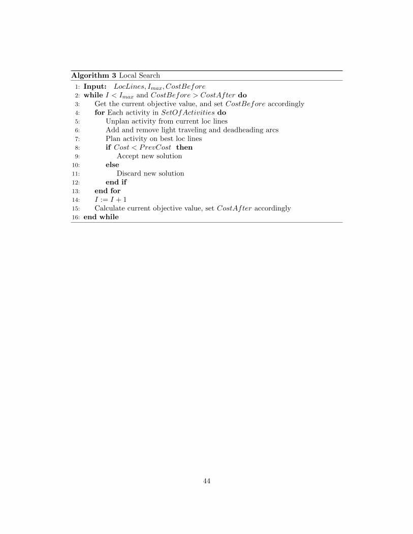
Algorithm 3 Local Search

1: Input: LocLines, Imax, CostBefore2: while I < Imax and CostBefore > CostAfter do3: Get the current objective value, and set CostBefore accordingly4: for Each activity in SetOfActivities do5: Unplan activity from current loc lines6: Add and remove light traveling and deadheading arcs7: Plan activity on best loc lines8: if Cost < PrevCost then9: Accept new solution

10: else11: Discard new solution12: end if13: end for14: I := I + 115: Calculate current objective value, set CostAfter accordingly16: end while

44

7 Computational Results

In this chapter, the results of the different solution approaches as described in

Chapter 6 are discussed. The different methods are programmed in Quintiq software.

All MIP formulations are solved by using CPLEX 12.5.1, which can be accessed via

the Quintiq software package. In general, the Quintiq software package is an object

oriented programming language, which is a mix between C++ and Java, which are

both object oriented programming languages. All methods are performed on a laptop

with 8.0 GB RAM memory and an Intel(R) Core(TM) i7-4800MQ CPU @ 2.70GHz

processor. The reported running times are all obtained using the same laptop, and

are hence comparable with each other.

The remainder of this chapter is divided as follows. In Section 7.1 different prob-

lem instances which will be used to investigate the quality of the different heuristics

are described. Afterwards, Section 7.2 describes the results for the smallest problem

instances, Section 7.3 the results for the middle sized problem instances and Section

7.4 the results of the real-size dataset. Section 7.5 investigates the robustness of the

solutions by changing the minimum turntime.

7.1 Generating different problem instances

In this section, two newly generated problem instances will be discussed. As de-

scribed before, it is important to generate smaller problem instances in order to eval-

uate the different heuristics and formulations. Also, several variants of the heuristics

can be tested before actually solving the real-life, and much larger, problem instance.

Hence, two additional problems were generated. The first problem contains only

250 activities, divided amongst ten different locations. This problem will be referred

to as the small problem. The second problem, a medium size problem, contains of

500 activities divided amongst 25 different locations. To avoid that a problem turns

out to be very hard or very easy to solve, we generate three different instances for

both cases.

For both problems, the different locations are denoted by an x and y coordinate.

Each of the x and y coordinates is assumed to be uniformly distributed on the interval

[0, 200]. The distance between a pair of locations will be calculated according to the

Euclidean distance, which is defined as given in Formula (22).

D(i, j) = D(j, i) =

√(xi − xj)2 + (yi − yj)2 (22)

45

Each of the activities is either passenger related, cargo related or a loc order.

The proportion of activities corresponding to one of the types is the same as given

in Table 5. Also, the average duration of the loc orders corresponds to the average

duration in Table 5. For the other activities, the duration is determined by assuming

an average speed, which is slightly higher for the passenger related activities.

The starting and ending location of the activities are randomly selected, where

each of the locations has the same probability of being selected. This may be a

difference with the real-life dataset, because with the real-life dataset there are certain

sets of locations which are connected more often than other sets of locations. For

example, one could think of a busy connection between two large cities, which will

be used more frequently than a connection between smaller locations. Although

the allocation of locations may be different, the problem instances are probably well

capable of investigating the quality of the different heuristics.

The set of available locomotive types and associated costs are exactly the same

as shown in Tables 2 - 4. The only difference lies in the number of locomotives which

are available. The number of available locomotives is adjusted such that the relative

number of available locomotives remains comparable with the real-life dataset. The

number of locomotives which is required depends mainly on the number of activities.

Since the smaller problem instances are daily problems, while the real-size problem

instance is a weekly problem, we should compare the number of activities per day.

The number of available locomotives can be determined based on the proportion of

activities in the smaller problem instances compared to the real-size problem instance.

All cost related parameters are the same, which is important when considering light

traveling or deadheading opportunities.

Each of the instances will be used to evaluate the results of the different heuristics.

Also, for the relax-and-fix heuristic and the greedy heuristic, multiple variants of the

heuristics are investigated. After that, the best performing approaches are applied

to the real-life dataset.

7.2 Results for the small problem instances

In this section, the results for the small problem will be discussed for each of the

heuristics separately. Furthermore, the results will be compared between the different

methods, and conclusions will be drawn from these results. First, the results for the

MIP formulations will be provided. For both formulations, all possible light traveling

arcs are generated. The results are depicted in Table 7 and Table 8.

46

Instance Runtime (s) Objective Value (e) Opt Gap (%) Gap (%) Variables Constraints

1 83 154,812.40 0.00 0.00 55,955 98,7452 296 205,463.97 0.00 0.00 55,820 98,3953 170 135,190.17 0.00 0.00 55,850 98,455

Table 7: Results for the locomotive based formulation

Instance Runtime (s) Objective Value (e) Opt Gap (%) Gap (%) Variables Constraints

1 10 157,350.00 1.64 0.00 104,388 203,2812 8 208,151.46 1.31 0.00 103,968 202,4413 8 138,015.26 2.09 0.00 104,040 202,825

Table 8: Results for the consist based formulation

In both Table 7 and Table 8, and in many of the following tables, the columns

Opt Gap (%), which is the optimality gap, and Gap (%) appear. The optimality

gap denotes the gap between the obtained solution and the optimal solution. More

formally, the optimality gap is calculated as given in Equation (23).

ε =zH − z∗

z∗· 100% (23)

In Equation (23), zH denotes the obtained solution with the current method,

while z∗ denotes the optimal solution. Note that for some larger problems, the

optimal solution is usually unknown. In this case, z∗ denotes the best lower bound

on the optimal solution.

The gap is only provided for both formulations. In case the optimal solution has

not been reached within the maximum computation time, the gap between this solu-

tion and the current best lower bound on the solution is provided. When calculating

the optimality gap in this case, z∗ is equal to the best lower bound after the maximum

computation time. Note that the optimality gap is an upper bound in this case, as

the optimal solution is always larger than z∗.

From Table 7, we conclude that all instances were solved to optimality within

5 minutes. The differences between the problem instances are rather large, as the cost

for instance 2 is about 50% higher than the cost for instance 3. This large difference

is due to the position of the different locations. For instance 2, the distances between

locations are larger compared to instance 3, which results in an increase in costs

associated to fulfilling these activities.

47

Table 8 shows that the computation time for the consist based formulation is

much shorter than for the locomotive based formulation, although the number of

variables and constraints is considerably higher. As explained before, the consist

based formulation is likely to provide non-optimal solutions, which is confirmed by

Table 8. Although the solution is non-optimal, the optimality gap is only 2.1% in

the worst case, which is relatively small. Comparing the number of variables and

constraints between both formulations, the consist based formulation has around

twice as many variables and constraints. This difference is due to the larger number

of consists compared to the number of locomotive types.

Second, the results for relax-and-fix heuristic will be provided. In Section 6.3,

two different approaches are described. Table 9 provides the results for the approach

where all variables are fixed in each iteration, while Table 10 corresponds to the

approach where only part of the variables are fixed.

StepSize (min) Subproblems (#) Instance Result R1 (s) Time (s) Objective Value (e) Opt Gap (%)

50 29

1Best 3 57 155,131.06 0.21

Average 3 58 155,206.58 0.26

2Best 3 61 206,049.55 0.29

Average 3 63 206,719.76 0.61

3Best 2 57 135,880.25 0.51

Average 2 58 136,254.38 0.79

100 15

1Best 5 37 155,131.06 0.21

Average 3 34 155,169.69 0.23

2Best 5 35 206,049.55 0.29

Average 7 39 206,478.20 0.50

3Best 2 33 135,540.80 0.26

Average 2 35 135,644.85 0.34

150 10

1Best 3 48 154,996.11 0.12

Average 4 36 155,142.00 0.21

2Best 15 38 206,361.41 0.44

Average 10 35 206,809.74 0.65

3Best 2 24 135,675.31 0.36

Average 2 24 135,913.51 0.54

250 6

1Best 8 22 155,100.46 0.19

Average 8 25 155,274.90 0.30

2Best 9 23 206,255.50 0.39

Average 17 32 206,274.31 0.40

3Best 2 17 135,398.74 0.15

Average 2 20 135,512.20 0.24

Table 9: Results for the relax-and-fix heuristic when fixing all variables in each iteration.The average values are obtained by performing ten different runs. R1 denotes the computationtime for the first subproblem

48

In Table 9, the relax-and-fix heuristic is solved for different values of StepSize.

For each instance, the time to solve the first subproblem, denoted by R1, and the

total computation time are provided. It is important to distinguish the first sub-

problem from the other subproblems, because the computation time of this iteration

will be considerably larger. In the first iteration, an initial solution needs to be ob-

tained, while in the following iterations part of the solution is already known. This

reduces the number of variables, but also the number of possible solutions. Hence,

the computation time per iteration decreases when the heuristic progresses.

StepSize (min) Subproblems (#) Instance Result R1 (s) Time (s) Objective Value (e) Opt Gap (%)

25 58

1Best 3 109 154,983.06 0.11

Average 3 111 155,027.68 0.14

2Best 2 109 206,919.04 0.71

Average 2 112 207,816.46 1.15

3Best 2 109 135,971.18 0.58

Average 2 113 136,178.92 0.73

50 29

1Best 2 63 154,904.11 0.06

Average 3 62 155,004.55 0.13

2Best 3 64 206,049.55 0.29

Average 8 72 206,748.19 0.63

3Best 2 66 135,540.80 0.26

Average 2 62 135,618.61 0.32

75 20

1Best 3 60 154,842.67 0.02

Average 3 56 154,937.60 0.08

2Best 12 54 206,338.14 0.43

Average 12 56 206,665.00 0.58

3Best 2 44 135,540.80 0.26

Average 2 44 135,675.15 0.36

125 12

1Best 16 43 155,108.00 0.19

Average 12 41 155,130.35 0.21

2Best 7 36 205,906.62 0.22

Average 12 42 206,106.17 0.32

3Best 2 31 135,398.74 0.15

Average 2 31 135,554.80 0.27

Table 10: Results for the relax-and-fix heuristic when only fixing half of the variables ineach iteration. The average values are obtained by performing ten different runs. R1 denotesthe computation time for the first subproblem

For each instance, the best solution and the average solution over ten runs are

reported. One might expect that the relax-and-fix heuristic gives the same solution

in every run, because every subproblem is solved to optimality. However, randomness

in solutions is possible because there are multiple solutions with the same objective

value. For example, the cost for loc orders is the same irrespective of the locomotive

49

type which fulfills the activity.

From Table 9, we see that the optimality gap generally decreases when the step

size becomes larger. Of course, solving larger subproblems at once leads to a solution

which is usually closer to the optimal solution, because more variables are fixed at

once. In some cases, this finding does not hold. An opposite finding might be due to

the division of activities among the subsets. Some activities will be important for ob-

taining a good solution, for example those activities which require long light traveling

arcs. The division of subsets could be such that these activities are divided ineffi-

ciently among the subsets, resulting in an increase in objective value. Consequently,

the computation time per iteration increases, due to a larger number of integer vari-

ables. Furthermore, the difference between the average objective value and the best

objective value is relatively small, in all cases smaller than 0.32%. This indicates that

the randomness which is involved has only limited effect on the objective value.

More interestingly, we can compare Table 9 and Table 10. As expected, the com-

putation time is about twice as large in case only part of the variables are fixed in

each iteration. The difference might be smaller in case many infeasibilities occur in

the approach where all variables are fixed, although there are almost no infeasibili-

ties for these smaller problem instances. On average, the optimality gap is slightly

lower with the second approach, although the differences are rather small. Overall,

both approaches manage to obtain solutions which are close to the optimal solution,

since the optimality gap is usually around or below 0.5%. For these smaller problem

instances, the best performance is achieved when larger subproblems are solved in

each iteration. Clearly, when the size of the problem instances increases, the com-

putation time to solve each of the larger subproblems becomes larger. Therefore, it

is important to note that the relax-and-fix heuristic is also performing well when the

subproblems are smaller.

Finally, the results for the greedy heuristic will be provided. Table 11 reports the

results for the small dataset. Just as with the relax-and-fix approach, the average

values and best values over ten runs are provided. Since there is randomness in the

order in which the activities are assigned, it is necessary to perform multiple runs to

investigate the average performance. Also, two different approaches for sequencing

activities are investigated: Method A denotes the method which sorts the activities

based on number of possible tractions, followed by number of possible locomotives

and finally randomly assigning activities with the same difficulty factor. Method B

corresponds with the sequence based on first sorting on the number of possible trac-

50

tions, followed by sorting on the starting time of the activity. Finally, the results

are split such that the objective after the greedy heuristic is provided, as well as the

results after the local search heuristic. Note that each run of the local search heuristic

uses the solution of the greedy heuristic as initial solution.

Greedy heuristic Local SearchMethod Instance Result Time (s) Objective (e) Opt Gap (%) Time (s) Objective (e) Opt Gap (%)

A

1Best 1 172,460.83 11.40 6 168,779.96 9.02

Average <1 177,539.52 14.68 7 171,434.45 10.74

2Best 1 238,684.30 16.17 8 230,275.71 12.08

Average <1 241,823.00 17.70 7 233,582.32 13.69

3Best 1 154,020.23 13.93 10 148,803.09 10.10

Average <1 157,138.64 16.24 7 151,383.71 11.98

B

1Best <1 172,204.36 11.23 8 167,014.00 7.88

Average <1 175,438.00 13.32 6 169,972.98 9.79

2Best <1 234,824.62 14.29 5 227,062.83 10.51

Average <1 236,804.26 15.25 5 229,458.35 11.68

3Best 1 153,557.44 13.59 9 146,155.92 8.11

Average <1 154,472.09 14.26 7 148,519.84 9.86

Table 11: Results for the greedy heuristic, separated before and after local search hasbeen applied. The average values are obtained by performing ten different runs. MethodA corresponds with the sequence based on the number of possible tractions, the number ofpossible locomotives which are able to fulfill the activity and after that a random sequencefor those activities which have the same factor. Method B corresponds to the sequence basedon the number of possible tractions, and based on the starting time afterwards

From Table 11, we can conclude that method B is outperforming method A, be-

cause it provides solutions with lower costs for every problem instance. As expected,

the greedy heuristic performs worse than the relax-and-fix heuristic in terms of the

objective value, with an optimality gap of around 15% in the worst case. However,

the weaker performance is compensated by a reduction in computation time, since

the greedy heuristic solves the problem instances within one second. As explained

before, the greedy heuristic can be improved by performing a local search heuristic.

On average, the local search heuristic took four iterations, resulting in an average

improvement of 4%. Even when the greedy heuristic and local search heuristic are

combined, the computation time does not exceed 10 seconds in any case, which is

considerably faster than the other approaches, except for the consist based formula-

tion.

The differences between the average objective values and the best objective values

are relatively large compared to the relax-and-fix method. Also, the differences are

larger for method A compared to method B. Clearly, larger differences are due to an

51

increase in randomness, which allows for a larger variety of solutions. With method A,

there are many activities with the same difficulty factor, hence every run of the greedy

heuristic has an order of assigning activities which is rather different from each other.

With method B however, the order of assignment is the same, and the randomness

is caused when two or more loc lines have the same cost when assigning the activity.

7.3 Results for the medium size problem instances

In this section, the results for the medium size problem instances are discussed.

First, both formulations are evaluated. Due to the increased size of the problem

instances, it is necessary to set a maximum computation time for the locomotive based

formulation. The computation time is bounded to be less than 2 hours. Table 12

reports the results for the locomotive based formulation, while Table 13 reports the

results for the consist based formulation.

Instance Runtime (s) Objective Value (e) Opt Gap (%) Gap (%) Variables Constraints

1 7,200 327,790.32 0.27 0.27 267,635 471,2752 7,200 347,989.25 0.24 0.24 267,770 471,5453 7,200 367,095.18 0.16 0.16 268,115 472,235

Table 12: Results for the locomotive based formulation. The optimality gap and gap aredetermined according to the best lower bound after 2 hours of computation time

Instance Runtime (s) Objective Value (e) Opt Gap (%) Gap (%) Variables Constraints

1 142 331,221.91 1.32 0.00 492,324 973,6532 61 351,508.19 1.25 0.00 492,648 974,3013 73 371,832.44 1.45 0.00 493,476 975,957

Table 13: Results for the consist based formulation

Table 12 shows that none of the problem instances were solved to optimality

within 2 hours. Contrary, the consist based formulation is still able to solve the

problem instances to optimality within only 3 minutes of computation time. The

optimality gap as reported in Table 13 is calculated compared with the best known

lower bound. This lower bound can be determined by the gap as reported in Table 12.

The optimality gap for the consist based formulation is comparable with the gaps

reported for the smaller problem instances.

52

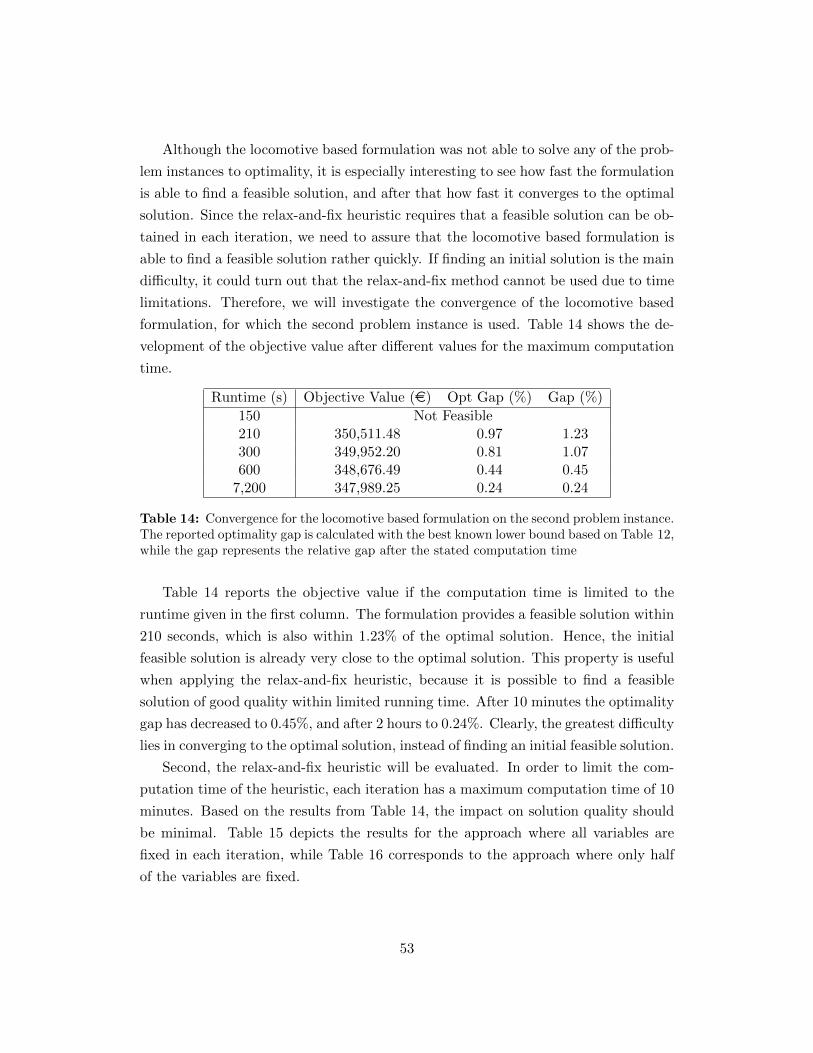
Although the locomotive based formulation was not able to solve any of the prob-

lem instances to optimality, it is especially interesting to see how fast the formulation

is able to find a feasible solution, and after that how fast it converges to the optimal

solution. Since the relax-and-fix heuristic requires that a feasible solution can be ob-

tained in each iteration, we need to assure that the locomotive based formulation is

able to find a feasible solution rather quickly. If finding an initial solution is the main

difficulty, it could turn out that the relax-and-fix method cannot be used due to time

limitations. Therefore, we will investigate the convergence of the locomotive based

formulation, for which the second problem instance is used. Table 14 shows the de-

velopment of the objective value after different values for the maximum computation

time.

Runtime (s) Objective Value (e) Opt Gap (%) Gap (%)

150 Not Feasible210 350,511.48 0.97 1.23300 349,952.20 0.81 1.07600 348,676.49 0.44 0.45

7,200 347,989.25 0.24 0.24

Table 14: Convergence for the locomotive based formulation on the second problem instance.The reported optimality gap is calculated with the best known lower bound based on Table 12,while the gap represents the relative gap after the stated computation time

Table 14 reports the objective value if the computation time is limited to the

runtime given in the first column. The formulation provides a feasible solution within

210 seconds, which is also within 1.23% of the optimal solution. Hence, the initial

feasible solution is already very close to the optimal solution. This property is useful

when applying the relax-and-fix heuristic, because it is possible to find a feasible

solution of good quality within limited running time. After 10 minutes the optimality

gap has decreased to 0.45%, and after 2 hours to 0.24%. Clearly, the greatest difficulty

lies in converging to the optimal solution, instead of finding an initial feasible solution.

Second, the relax-and-fix heuristic will be evaluated. In order to limit the com-

putation time of the heuristic, each iteration has a maximum computation time of 10

minutes. Based on the results from Table 14, the impact on solution quality should

be minimal. Table 15 depicts the results for the approach where all variables are

fixed in each iteration, while Table 16 corresponds to the approach where only half

of the variables are fixed.

53

StepSize (min) Subproblems (#) Instance Result R1 (s) Time (s) Objective Value (e) Opt Gap (%)

50 29

1Best 171 588 328,559.06 0.51

Average 161 546 329,317.72 0.74

2Best 182 591 349,655.71 0.72

Average 135 549 349,984.45 0.81

3Best 96 467 368,529.24 0.56

Average 94 473 369,199.85 0.73

100 15

1Best 160 406 328,278.89 0.42

Average 172 434 328,526.28 0.50

2Best 141 385 349,554.96 0.69

Average 143 406 349,915.46 0.79

3Best 161 529 368,177.33 0.45

Average 150 425 368,484.87 0.53

150 10

1Best 155 422 328,560.45 0.51

Average 146 390 328,797.16 0.58

2Best 600 964 349,246.24 0.60

Average 587 937 349,391.03 0.64

3Best 137 370 368,219.65 0.46

Average 125 390 368,395.40 0.51

250 6

1Best 312 483 327,894.69 0.30

Average 276 471 328,301.39 0.43

2Best 600 926 348,716.61 0.45

Average 575 1,008 348,912.24 0.51

3Best 124 512 368,177.66 0.45

Average 134 445 368,639.63 0.58

Table 15: Results for the relax-and-fix heuristic where all variables are fixed in each iteration.R1 denotes the computation time of the first subproblem. The average values are obtainedby performing ten different runs

Both approaches of the relax-and-fix heuristic show comparable results with those

from the smaller problem instances. The approach where only part of the variables

is fixed provides slightly better results, and the computation time is about twice

as large. From both Table 15 and Table 16, it becomes clear that solving the first

subproblem takes considerably more time than solving the other subproblems. In

the first subproblem, an initial feasible solution should be obtained. In following

iterations, part of the variables is already fixed, which decreases the solution space

and will lead to a decrease in computation time.

The computation time for each problem instance is more volatile compared to

the smaller dataset. For example, with a time step of 150 minutes, the first problem

instance is solved in 390 seconds while the second problem instance takes almost

1,000 seconds. There are some instances for which solving the MIP takes more time,

and the differences in computation time will increase once the problem instances

54

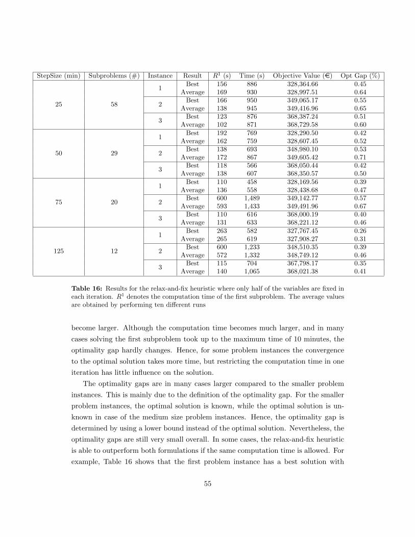
StepSize (min) Subproblems (#) Instance Result R1 (s) Time (s) Objective Value (e) Opt Gap (%)

25 58

1Best 156 886 328,364.66 0.45

Average 169 930 328,997.51 0.64

2Best 166 950 349,065.17 0.55

Average 138 945 349,416.96 0.65

3Best 123 876 368,387.24 0.51

Average 102 871 368,729.58 0.60

50 29

1Best 192 769 328,290.50 0.42

Average 162 759 328,607.45 0.52

2Best 138 693 348,980.10 0.53

Average 172 867 349,605.42 0.71

3Best 118 566 368,050.44 0.42

Average 138 607 368,350.57 0.50

75 20

1Best 110 458 328,169.56 0.39

Average 136 558 328,438.68 0.47

2Best 600 1,489 349,142.77 0.57

Average 593 1,433 349,491.96 0.67

3Best 110 616 368,000.19 0.40

Average 131 633 368,221.12 0.46

125 12

1Best 263 582 327,767.45 0.26

Average 265 619 327,908.27 0.31

2Best 600 1,233 348,510.35 0.39

Average 572 1,332 348,749.12 0.46

3Best 115 704 367,798.17 0.35

Average 140 1,065 368,021.38 0.41

Table 16: Results for the relax-and-fix heuristic where only half of the variables are fixed ineach iteration. R1 denotes the computation time of the first subproblem. The average valuesare obtained by performing ten different runs

become larger. Although the computation time becomes much larger, and in many

cases solving the first subproblem took up to the maximum time of 10 minutes, the

optimality gap hardly changes. Hence, for some problem instances the convergence

to the optimal solution takes more time, but restricting the computation time in one

iteration has little influence on the solution.

The optimality gaps are in many cases larger compared to the smaller problem

instances. This is mainly due to the definition of the optimality gap. For the smaller

problem instances, the optimal solution is known, while the optimal solution is un-

known in case of the medium size problem instances. Hence, the optimality gap is

determined by using a lower bound instead of the optimal solution. Nevertheless, the

optimality gaps are still very small overall. In some cases, the relax-and-fix heuristic

is able to outperform both formulations if the same computation time is allowed. For

example, Table 16 shows that the first problem instance has a best solution with

55

an optimality gap of 0.26%, which is smaller than the optimality gap of 0.27% as

reported in Table 12.

Although the approach where all variables are fixed seems to provide better re-

sults, mainly because it is faster and the solution quality is comparable, we will still

use both approaches on the real-size dataset. With the approach where all variables

are fixed in each iteration, infeasibilities occurred quite often, especially at one of the

last subproblems. Because the size of the subproblems is still quite small, the influ-

ence of infeasibilities is limited. However, the consequences for the real-size dataset

could be more severe and therefore considering both approaches can be justified.

Finally, we will discuss the results for the greedy and local search heuristics. Just

as with the small problem instances, the results are reported separately for both

heuristics, and the same two approaches for sequencing the activities are considered.

Table 17 shows the results for the greedy and local search heuristics, for which the

average and best solutions over ten runs are reported.

Greedy heuristic Local SearchMethod Instance Result Time (s) Objective (e) Opt Gap (%) Time (s) Objective (e) Opt Gap (%)

A

1Best 4 376,554.82 15.19 50 366,366.73 12.07

Average 4 383,857.91 17.42 48 369,031.42 12.89

2Best 3 400,153.63 15.27 53 384,423.86 10.74

Average 3 404,679.99 16.57 45 387,454.42 11.61

3Best 4 422,965.65 15.40 57 404,350.70 10.32

Average 4 426,991.37 16.50 43 409,422.63 11.70

B

1Best 5 375,656.60 14.91 64 362,729.22 10.96

Average 5 377,948.48 15.61 58 365,815.74 11.90

2Best 4 392,324.66 13.01 59 381,448.04 9.88

Average 4 396,909.25 14.33 44 385,102.43 10.93

3Best 5 415,809.46 13.45 43 404,199.22 10.28

Average 5 417,958.38 14.03 47 405,801.20 10.72

Table 17: Results for the greedy heuristic and local search heuristic. Method A correspondswith the sequence based on the number of possible tractions, the number of possible locomo-tives which are able to fulfill the activity and after that a random sequence for those activitieswhich have the same factor. Method B corresponds to the sequence based on the number ofpossible tractions, and based on the starting time afterwards

Table 17 shows comparable results with the results for the smaller problem in-

stances. Method B is outperforming method A for all problem instances, for both

the greedy heuristic as well as the local search heuristic. Therefore, we will only

apply method B on the real-size dataset, because method A does not provide better

results in any case. Just as with the smaller problem instances, the combination of

56

the greedy heuristic and the local search heuristic is faster than the other methods.

In this case, the computation time is also lower compared to the consist based for-

mulation. It is to be expected that the difference in computation time will become

larger once the problem instances are getting larger, such that the greedy heuristic is

the fastest heuristic on one hand, but resulting in the largest optimality gaps on the

other hand.

7.4 Results for the real-life dataset

In this section, the results for the real-life dataset are provided. As explained in

the previous sections, not all different variants of the heuristics will be investigated.

For both formulations, all different approaches for generating light traveling arcs

(see Section 6.1.1) are investigated. For the greedy heuristic, only the approach where

the order of assignment is based on the number of possible tractions, followed by

the starting time is evaluated. The other proposed approach turned out to provide

worse results for all problem instances. Because the volatility in objective values

turned out to be rather large, the results are reported after performing ten different

runs. Finally, for the relax-and-fix heuristic both approaches will be investigated,

mainly to investigate the effect of infeasibilities occurring in either of the approaches.

Considering the small relative differences between various runs for the same setting

of the StepSize parameter, we will only use one run for each of the values of the

StepSize parameter.

Due to the large size of the dataset, and because of the enormous amount of light

traveling arcs, it turned out that the available 8 GB of memory was insufficient. The

results as reported are obtained by solving the problems on an online server, which

provided sufficient memory. In the worst case, when generating all light traveling

arcs and solving the consist based formulation, up to 70 GB of memory was required.

First, we start by evaluating the performance of both MIP formulations. For both

formulations, the computation time is limited to 10 hours. In Table 18 the results for

the locomotive based formulation are shown for each of the approaches to generate

the light traveling arcs. Table 19 reports the results for the consist based formulation.

From Table 18, we can conclude that the locomotive based formulation is not able

to solve any of the approaches to optimality within 10 hours of computation time.

Further, the number of variables is very large, exceeding ten million variables in case

all light traveling arcs were generated. The performance of the different approaches

for generating light traveling arcs are widespread. The first approach when arcs are

57

Method Runtime (s) Objective Value (e) Opt Gap (%) Gap (%) Variables Constraints

All Arcs 36,000 5,091,774.98 0.39 0.39 10,512,985 18,436,629Approach A Not Feasible 1,445,710 2,538,159Approach B 36,000 5,422,303.25 6.91 0.45 877,800 1,541,599Approach C 36,000 5,134,845.88 1.24 0.32 2,009,075 3,527,754

Table 18: Results for the locomotive based formulation. Approach A denotes the casewhere only light traveling arcs are added based on the in and outflow of locomotives in eachlocation. Approach B only adds arcs between those locations which are connected by anactivity. Finally, Approach C combines the arcs of both approaches A and B

Method Runtime (s) Objective Value (e) Opt Gap (%) Gap (%) Variables Constraints

All Arcs 17,237 5,141,540.74 1.41 0.00 19,046,844 38,001,689Approach A Not Feasible 2,651,976 5,211,953Approach B 36,000 5,533,956.26 9.11 0.02 1,623,216 3,154,433Approach C 35,603 5,203,757.13 2.60 0.00 3,674,928 7,257,857

Table 19: Results for the consist based formulation. Approach A denotes the case where onlylight traveling arcs are added based on the in and outflow of locomotives in each location.Approach B only adds arcs between those locations which are connected by an activity.Finally, Approach C combines the arcs of both approaches A and B

only added based on flow of locomotives turned out to be infeasible. Apparently, there

are some essential variables omitted which are required to obtain a feasible solution.

The second approach, which adds only arcs between locations which are connected

by activities, succeeds in finding a feasible solution. Since the second method is able

to find a feasible solution, combining both approaches should result in a feasible

solution as well. This third approach has still a limited number of variables, while

the optimality gap is only 1.24% compared to an optimality gap of 6.91% with the

second approach. The third approach may be useful when applying the relax-and-fix

heuristic, because of the smaller number of variables, while the optimality gap is

rather small.

Table 19 shows that the consist based formulation is able to solve the problem

to optimality for the approaches with all light traveling arcs and the third approach,

which combines the first and second approach. The gap between the solution obtained

by the consist based formulation compared to the solution with the locomotive based

formulation is comparable with the medium size problem instances, usually around

1.5%. The second approach does not yield an optimal solution within 10 hours, which

is remarkable since the problem size is smallest when applying the second approach.

58

However, as the large gap already indicates, there are relatively few light traveling arcs

which makes finding an initial feasible solution harder. Therefore, the consist based

formulation is not able to find an optimal solution within 10 hours of computation

time.

We notice that the number of variables and constraints is extremely large with

the consist based formulation, which is a drawback of this method. Especially when

all light traveling arcs are considered, the number of variables is close to 20 million

and there are 38 million constraints. Hence, solving this problem requires more

memory than which may be available in many cases. Additionally, even initializing

all variables and creating all constraints takes up to 30 minutes already. On the other

hand, the formulation is able to solve the problem quicker, and even able to reach

optimality in many cases.

Although the results of the formulations are still quite well, the large computation

times are a serious drawback. Especially in real-life situations, there are often cases

when a schedule needs to be obtained quickly. Therefore, investigating the quality

of the heuristics is also essential. First, the results for the relax-and-fix heuristic

will be reported. To limit the computation time of this heuristic, each iteration is

stopped when either the relative difference is smaller than 0.5% or after one hour

of computation time. When all light traveling arcs are included, this limitation of

computation time did not result in any feasible solutions. Even when the maximum

time for an iteration was increased to 2 hours, still no feasible solution could be

obtained. Therefore, the results will be based on the third approach, which combines

the arcs based on locations and based on flow of locomotives. Table 20 depicts the

results for the approach where all variables are fixed in each iteration, while Table 21

reports the results when only part of the variables are fixed in each iteration.

StepSize (min) Subproblems (#) R1 (s) Time (s) Objective Value (e) Gap (%) Opt Gap (%)

336 30 546 16,245 5,180,427.14 1.21 2.14504 20 840 18,307 5,152,782.05 0.67 1.59672 15 Not Feasible

1,008 10 Not Feasible2,016 5 Not Feasible

Table 20: Results for the relax-and-fix heuristic where all variables are fixed in each iteration.R1 denotes the computation time of the first subproblem

59

StepSize (min) Subproblems (#) R1 (s) Time (s) Objective Value (e) Gap (%) Opt Gap (%)

168 60 746 32,412 5,172,529.36 1.06 1.98252 40 834 17,443 5,169,159.33 0.99 1.92336 30 855 13,599 5,150,220.83 0.62 1.54504 20 1,201 11,738 5,148,960.53 0.60 1.52

1,008 10 2,000 8,012 5,146,863.92 0.55 1.48

Table 21: Results for the relax-and-fix heuristic where only part of the variables are fixedin each iteration. R1 denotes the computation time of the first subproblem

Table 20 shows that the relax-and-fix heuristic is only able to obtain feasible

solutions when the size of the subproblems is smaller. Infeasibility for the cases where

the size of these subproblems is larger is caused by infeasibilities at the end of the

heuristic. In each of these cases, a sequence of infeasibilities resulted in solving almost

the entire problem at once, which could not been done within 1 hour of computation

time. Moreover, it is also not desired to solve such large subproblems, simply because

there is no advantage in using the heuristic in the first place and one could just solve

the complete locomotive based formulation instead.

The two cases with smaller subproblems result in feasible solutions which are close

to the optimal solution. The gap denotes the difference with the objective value with

the same set of light traveling arcs, while the optimality gap denotes the difference

with the best known lower bound. The gaps are 1.21% and 0.67%, which is larger

than for the smaller problem instances. The increase in gap is due to two factors.

First, the locomotive based formulation could not reach optimality, and the gap of

0.32% is larger than for the medium and smaller problem instances. Second, the

stopping criteria influence the final solution. Since each iteration is stopped when

the solution is within 0.5% of the optimal solution, the overall gap increases.

As infeasibilities turn out to have large impact on solutions for the relax-and-fix

heuristic on a larger dataset, it is interesting to see if the performance improves once

only part of the variables are fixed. This case is depicted in Table 21. We notice

that this approach provides feasible solutions for all different parameter settings of

StepSize. Further, we observe an interesting pattern: when the size of the subprob-

lems increases, the time of the first subproblem increases, while the total computation

time decreases quite rapidly. This is due to a decrease in the number of subproblems

which needs to be solved. Though, the decrease in total time is larger than for the

small and medium size problem instances. The main explanation for this difference

lies in the size of the problem. In each iteration of the heuristic, all variables and

60

constraints have to be initialized. For the smaller instances this initialization time

is negligible, but this initialization time becomes more significant for the larger in-

stances. Hence, the advantage of having small subproblems which could be solved

quickly is annihilated by the initialization time in each iteration.

Looking at the objective values tells that the optimality gaps decrease when the

size of the subproblems increases. This pattern could also be observed on the smaller

problem instances. The optimality gap is around 1.5% if the subproblems get suffi-

ciently large. The obtained solution is comparable with the solution of the consist

based formulation when all light traveling arcs are considered, but the computation

time can be halved by using the relax-and-fix heuristic.

Finally, the results for the greedy heuristic and local search heuristic will be

provided. As said before, the results are based on ten different runs. Also, only the

approach where the activities are assigned based on starting time is used. Table 22

summarizes the results for the real-size dataset.

Greedy heuristic Local SearchResult Time (s) Objective (e) Opt Gap (%) Time (s) Objective (e) Opt Gap (%)

Best 1,856 6,063,725.69 19.55 6,723 5,809,936.77 14.70Average 2,176 6,102,139.87 20.31 7,129 5,821,909.62 14.79

Table 22: Results for the greedy heuristic and local search heuristic. The reported averagesare based on ten different runs

From Table 22, we observe that the optimality gap with the greedy heuristic

is quite large, also in comparison with the medium and smaller problem instances.

The increase of optimality gap is caused by several factors. Firstly, the increase in

number of locations and the specific schedule require many light traveling arcs or

deadheading activities. Secondly, due to the possible tractions of the activities, there

are some locomotive types for which each locomotive has to fulfill many activities.

In combination with the first statement, the use of light traveling arcs can become

inefficient. The greedy heuristic is still able to assign all activities within 40 minutes,

which is considerably faster than all other methods.

The local search heuristic leads to large improvements, on average lowering the

optimality gap with 5.5%. The achieved improvement with the local search heuristic

is on average larger than with the medium and small problem instances, although this

is probably due to weaker initial solutions which allow for larger improvements. The

combination of the greedy heuristic and three iterations of the local search heuristic

61

takes around 2.5 hours, which is still considerably long if one wants to obtain a

reasonable schedule quickly. One clear opportunity lies in reducing the number of

iterations of the local search heuristic. Figure 2 shows the average optimality gap

after each iteration of the local search heuristic.

0 1 2 3 414

16

18

20

22

Iteration

Op

tim

alit

yG

ap(%

)

Figure 2: The development of the optimality gap after a number of iterations of the localsearch heuristic. The optimality gap is the average optimality gap determined over tendifferent runs of the greedy and local search heuristic

Figure 2 shows that the largest improvement of the optimality gap has been

achieved in the first iteration of the local search heuristic. In this iteration, the

optimality gap has already decreased by 4.0%. The second and third iteration only

account for 1.5% decrease in optimality gap. Hence, if the main goal lies in finding

a quick solution, performing only one iteration of the local search iteration would be

the most preferred option. In this case, a solution can be obtained within 80 minutes,

which has an optimality gap just over 16%.

We will end this section with some concluding remarks about the different meth-

ods. Both formulations provide solutions with the lowest optimality gaps. However,

the computation time for these methods is large, and both methods require a large

available memory. The relax-and-fix heuristic works well, especially if part of the

variables are fixed in each iteration. The optimality gap is also small, smaller than

2% even in the worst case. However, this heuristic was not able to find solutions for

the case where all light traveling arcs were considered. The computation time is also

smaller than for both formulations, but larger than for the greedy heuristic and local

62

search heuristic. This final method is the fastest, but also results in a solution with

the largest optimality gap. This method is especially useful if one wants to obtain

a solution quickly. In general, a trade-off between solution quality and computation

time needs to be made. It seems that the relax-and-fix heuristic provides the best re-

sults, because if the size of the subproblems is appropriately chosen, the computation

time remains limited while the optimality gap remains small.

7.5 Varying the turntime

In this section the objective value is compared when different minimum turntimes

are used. Previously, the time between two consecutive operations performed by a

locomotive had to be at least as large as the minimum turntime at that location. How-

ever, in real-life it is often desired that the time between two consecutive operations is

much larger than this minimum time. Increasing the turntime is especially important

when delays are taken into account. Clearly, if there is an activity for which there is

a delay of 30 minutes and the time between two activities is only 20 minutes, then

there will be a delay on the next activity as well. Hence, by increasing the turntimes

the schedule will be more robust against delays. Table 23 evaluates the performance

of all small and medium sized problem instances when the minimum turntime is in-

creased to 15, 30, 45 or 60 minutes, respectively. The results are evaluated on the

consist based formulation, which is able to solve the problem instances quickly.

Small Medium

Minimum turntime Instance Objective (e) Gap (%) Objective (e) Gap (%)

151 157,440.61 0.06 331,343.69 0.042 208,391.96 0.12 352,062.79 0.163 138,018.37 0.002 371,945.14 0.03

301 157,851.54 0.32 332,603.11 0.422 209,812.54 0.80 353,357.64 0.533 138,576.90 0.41 373,291.61 0.39

451 158,193.06 0.54 334,321.60 0.942 211,037.41 1.39 354,912.71 0.973 139,057.52 0.76 374,187.83 0.63

601 158,980.83 1.04 335,316.96 1.242 211,752.53 1.73 356,072.06 1.303 139,721.68 1.24 376,808.30 1.34

Table 23: Performance of the different problem instances on the consist based formulationwhen the minimum turntime is varied

63

Table 23 shows the gap for different values of the minimum turntime. The gap

denotes the difference between the optimal solution as obtained with the consist based

formulation (see Table 8 and Table 13) and the solution obtained with the adjusted

minimum turntimes. An important observation is the low increase in optimality value

when the minimum turntime is increased. This means that the current schedule is

such that there are few operations which are scheduled close after each other. An

explanation might rely on the construction of the light traveling arcs. Since the light

traveling arcs originate at the latest possible time at each location, there are many

light traveling arcs which can be used even when the minimum turntime is increased.

The effect on changing the minimum turntime for the real-size dataset is likely to

be comparable with the effect as observed on the smaller datasets. Possibly, the gap

increases slightly, because we already noticed that the schedule tends to be denser

for some of the locomotive types. By increasing the minimum turntimes, some of the

routes are likely to become infeasible. Since there are few other opportunities, there

could appear some cases for which there are inefficient connections which have to be

made to obtain a feasible solution.

64

8 Conclusion

In this thesis, a large real-life problem instance of the Locomotive Assignment

Problem (LAP) has been solved. In the past decade, the use of optimization models

in the field of rail transport has increased immensely. The LAP is one of the most

important problems in railway scheduling. The dataset which is considered for this

study is large compared to data instances in other papers, and especially the need of

light traveling and deadheading opportunities increases the difficulty of the problem.

To solve this problem, we proposed two different multi-commodity flow formula-

tions and two different heuristics. The commodities in the formulations correspond

either to specific locomotive types or consists. For both formulations, a large time-

space network is used. Because there is an enormous amount of variables and con-

straints in both formulations, the use of heuristic approaches could be justified. The

large size of the network is mainly due to the light traveling arcs, and therefore several

heuristic approaches for creating light traveling arcs are provided.

The first heuristic is a relax-and-fix heuristic. A relax-and-fix heuristic solves the

multi-commodity formulation iteratively, where in each iteration part of the variables

is forced to be integer, while many variables are relaxed. Two different approaches

for fixing the variables in each iteration were discussed. In the first approach, all

variables which were forced to be integer in the previous iteration are fixed. The

second approach fixes only half of these variables. The first approach might result

in infeasible subproblems at some moment of the heuristic, which could be solved by

fixing a smaller part of the variables. Although the second approach requires twice

as many iterations, the number of infeasibilities decreases because the subproblems

become less restricted.

The second heuristic is a greedy heuristic, which is extended with a 1-opt local

search heuristic. The greedy heuristic starts with finding an efficient order for as-

signing the activities. Afterwards, the activities are assigned such that the costs are

minimized after assigning each of the activities. Once all activities are assigned, it is

highly unlikely that the optimal solution has been reached. To improve the solution,

the solution following from the greedy heuristic is used as initial solution of the local

search heuristic. The local search heuristic aims to improve the solution, by making

small local changes and accepting a neighbouring solution if it results in a decrease

of the total costs.

Next to the real-size dataset, some smaller problem instances were created to in-

vestigate and compare different approaches of the heuristics. For the smallest dataset,

65

containing only 250 activities divided among 10 locations, the locomotive based for-

mulation is able to reach the optimal solution within 5 minutes. All other approaches

are quicker, but do not manage to obtain the optimal solution. The consist based

formulation and combination of the greedy heuristic with the local search heuristic

are fastest, but result in an optimality gap of 1.5% and 10%, respectively. The relax-

and-fix heuristic is faster than the locomotive based formulation, but faces optimality

gaps between 0.1% and 1.1%, dependent on the size of the subproblems. Therefore

the use of the locomotive based formulation is recommended on smaller problem

instances.

The medium sized problem instances contain 500 activities, divided among 25

locations. It turned out that the locomotive based formulation was not able to solve

any of the problem instances within 3 hours. Although the obtained solutions after 3

hours of computation time are better than the objective values of the other methods,

faster alternatives may be preferred in this case. The consist based formulation

solves the instances within 2 minutes, and the resulting optimality gaps are around

1.3%. The relax-and-fix heuristic takes longer, usually around 10 minutes, but the

optimality gaps are lower, in many cases around 0.5%. The greedy heuristic is the

fastest method, but has optimality gaps between 10% and 12%. For the medium

sized problem instances, both the consist based formulation as well as the relax-and-

fix method are the recommended solution approaches.

The real-size dataset, containing almost 4,200 activities, turned out to be fairly

challenging, especially because the available memory on the laptop was insufficient.

Both formulations were limited to 10 hours of computation time. Also, different ap-

proaches for generating light traveling arcs were considered. The locomotive based

formulation could not solve any of the approaches to optimality, leaving gaps around

0.4%. The consist based formulation was usually able to solve the problem to op-

timality, but took over 5 hours in any case. The gaps between both formulations

were comparable with the gaps as observed with the smaller problem instances. The

relax-and-fix heuristic showed different results based on which approach with respect

to fixing variables was applied. In case all variables were fixed, infeasibilities in some

iterations of the heuristic caused problems. However, the approach where only half of

the variables are fixed performed very well. With some larger subproblems, a solution

within 1.5% of optimality could be obtained within 2.5 hours.

The combination of the greedy heuristic and local search heuristic could obtain

a solution within 80 minutes of computation time. However, the solutions face opti-

66

mality gaps close to 15%, which is substantially large compared to the relax-and-fix

heuristic. In general, the relax-and-fix heuristic where only part of the variables are

fixed is recommended. However, we need to mention that if the size of the problem

would increase, the greedy heuristic would still be able to find a solution in limited

time. This is questionable for all other solution approaches. Also, from a practical

point of view, if a solution has to be found quickly, the greedy heuristic is able to

provide a feasible solution within 40 minutes of computation time.

67

9 Further Research

In different stages of this research, some further research would be required. First,

some ideas for further research for both heuristics are provided. After that, some more

general ideas for further research are discussed.

With the real-size dataset, the light traveling opportunities turned out to be

a point of interest. Generating all possible light traveling arcs results in a very

large network, which causes memory issues and resulted in problems when solving

the formulations. Therefore, we proposed different heuristics to generate a smaller

number of possible light traveling arcs. Although the results were satisfactory, there is

some room for improvement in generating these arcs. Generating light traveling arcs

should become more dependent on the characteristics of the dataset. For example,

with one of the proposed methods, it turned out that the problem became infeasible.

This infeasibility is the result of leaving out some important light traveling arcs

which are required to provide feasible solutions. Hence, more detailed research on

the dataset could show which light traveling arcs are of vital importance for generating

feasible solutions.

The relax-and-fix heuristic turned out to perform well on the large dataset, espe-

cially in case only half of the variables were fixed in each iteration. It is interesting to

investigate different proportions of variables which are fixed. For example, fixing 34

of the variables in each iteration might be sufficient to avoid infeasibilities, while less

iterations are required compared to the case where half of the variables were fixed.

Further, we noticed that the computation time for solving the first subproblem is

larger than for the following subproblems. Therefore, it might be beneficial to solve

a smaller first subproblem, and increase the step size in following problems.

The idea of dividing the problem into smaller subproblems which are solved it-

eratively seems to be rather efficient. With the relax-and-fix heuristic, the division

of the subsets is based on the starting time of an arc. It might be interesting to

investigate different decomposition criteria. One intuitive criterion would rely on the

possible tractions of each of the activities, such that the division is based on different

types of locomotives. In this case, it is clear how the activity arcs should be divided

among the different subsets. However, dividing the other arcs might be harder, as

these arcs are not specifically related to the locomotive type.

The greedy heuristic in combination with the local search heuristic is the fastest

heuristic of all approaches, however the solution quality turned out to be rather poor.

One shortcoming of the method lies in the circularity restriction. With the greedy

68

heuristic, we forced that each loc line was circular, hence each locomotive could

perform the same loc line every week. This is a more restrictive assumption than the

assumption that the entire schedule should be circular. One possible approach may

execute the greedy heuristic as it is proposed right now, and updates the schedule

afterwards by applying a heuristic approach to find which arcs can be removed and

result in the largest improvement in total costs. This heuristic considers pairs of

loc lines of the same locomotive type. Then, we can add arcs between the ending

location of one loc line to the starting location of the other loc line, and remove the

currently existing arcs. Then, the difference in costs between both routes should be

determined and the combinations with the largest savings should be implemented.

Note that once this approach is implemented it will be harder to apply the local search

heuristic, because we should also take into account that the entire solution should

remain circular, while each of the separate loc lines are not forced to be circular.

Next to the heuristic related improvements, we will also indicate some more gen-

eral ideas for further research. First of all, the proposed methods provide a static

solution of the problem, since for example maintenance, breakages of locomotives and

delays are not taken into account. Clearly, once stochastic factors are considered, it

becomes much harder to solve the problem within reasonable time.

Another crucial element in the LAP is the light traveling arcs. With respect to the

light traveling arcs in the current solutions, we had to make some assumptions which

require further investigation. When generating the light traveling arcs, we assumed

that an arc could originate at every moment during the week. However, this may be

infeasible in real-life applications, simply because there are certain numbers of crew

members required to fulfill these activities. One can imagine that it is not desired

to have many light traveling arcs taking place during night time. Also, there might

be some locations which do not allow any light traveling activities. We also had to

make assumptions about the duration of the light traveling arcs. Hence, additional

information about these light traveling arcs is necessary if one wants to obtain a

solution which is desirable in real-life applications.

Finally, we notice that the current allocation of activities results in a schedule

which is rather unbalanced; i.e. there are some locomotives for which the schedule

is very dense, while there are other locomotives of the same locomotive type which

only contain few activities. Clearly, the unbalanced solution is the result of the

cost structure, as the objective does not take the allocation of activities over the

different locomotives into account. In reality, unbalanced schedules may be undesired,

69

especially with respect to breakages and possible delays. Suppose there is a locomotive

with a very dense schedule which breaks down while performing an activity. This

breakage also affects other activities, since this locomotive has many other activities

which it needs to fulfill. One could solve this issue by adding another factor to the

objective value, for example to limit the total time a locomotive is allowed to be

active, or to penalize short turntimes between two activities.

70

References

Ahuja, R.K., Magnanti, T.L., Orlin, J.B. 1993. Network Flows: Theory, Algorithms

and Applications. Prentice-Hall, Englewood Cliffs.

Ahuja, R.K., Liu, J., Orlin, J.B., Sharma, D., Shughart, L.A. 2002. Solving real-

life locomotive scheduling problems. Working Paper 4389-02, MIT Sloan School of

Management, 34 pages.

Booler, J.M.P. 1980. The solution of a railway locomotive scheduling problem.

The Journal of the Operational Research Society 31(10), 943-948.

Cordeau, J.F., Gendreau, M., Laporte, G. 1997. A tabu search heuristic for periodic

and multi-depot vehicle routing problems. Networks 30(2), 105-119.

Cordeau, J.F., Toth, P., Vigo, D. 1998. A survey of optimization models for train

routing and scheduling. Transportation Science 32(4), 380-404.

Cordeau, J.F., Soumis, F., Desrosiers, J. 2000. A Benders decomposition approach for

the locomotive and car assignment problem. Transportation Science 34(2), 133-149.

Even, S., Itai, A., Shamir, A. 1976. On the complexity of timetable and multi-

commodity flow problems. SIAM Journal on Computing 5(4), 691-703.

Florian, M., Bushell, G., Ferland, J., Guerin, G., Nastansky, L. 1976. The engine

scheduling problem in a railway network. INFOR 14(2), 121-138.

Forbes, M.A., Holt, J.N., Watts, A.M. 1991. Exact solution of locomotive scheduling

problems. The Journal of the Operational Research Society 42(10), 825-831.

Fugenschuh, A., Homfeld, H., Huck, A., Martin, A. 2006. Locomotive and wagon

scheduling in freight transport. 6th Workshop on Algorithmic Methods and Models

for Optimization of Railways (ATMOS’06), 14 pages.

Ho, W., Ho, G.T.S., Ji, P., Lau, H.C.W. 2008. A hybrid genetic algorithm for

the multi-depot vehicle routing problem. Engineering Applications of Artificial

Intelligence 21(4), 548-557.

Kasalica, S., Mandic, D., Vukadinovic, V. 2013. Locomotive assignment optimization

including train delays. Promet - Traffic & Transportation 25(5), 421-429.

71

Noble, D.H., Al-Amin, M., Mills, R.G.J. 2001. Production of locomotive rosters for

a multi-class multi-locomotive problem. The Journal of the Operational Research

Society 52(11), 1191-1200.

Noori, S., Ghannadpour, S.F., 2012. Locomotive assignment problem with train

precedence using genetic algorithm. Journal of Industrial Engineering International

8(9), 1-13.

Piu, F. 2011. A mixed integer programming approach to the locomotive assignment

problem. Ecole Polytechnique Federale de Lausanne, 42 pages.

Piu, F., Speranza, M.G. 2014. The locomotive assignment problem: a survey on

optimization models. International Transactions in Operational Research 21(3),

327-352.

Powell, W.B., Bouzaiene-Ayari, B. 2006. Approximate dynamic programming

for locomotive optimization. Department of Operations Research and Financial

Engineering, Princeton University, 8 pages.

Renaud, J., Laporte, G., Boctor, F.F. 1996. A tabu search heuristic for the multi-

depot vehicle routing problem. Computers & Operations Research 23(3), 229-235.

Rouillon, S., Desaulniers, G., Soumis, F. 2006. An extended branch-and-bound

method for locomotive assignment. Transportation Research Part B 40(5), 404-423.

Teichmann, D., Dorda, M., Golc, K., Bınova, H. 2015. Locomotive assignment prob-

lem with heterogeneous vehicle fleet and hiring external locomotives. Mathematical

Problems in Engineering, Article ID 583909, 7 pages.

Vaidyanathan, B., Ahuja, R.K., Liu, J., Shughart, L.A. 2008. Real-life locomotive

planning: new formulations and computational results. Transportation Research

Part B: Methodological 42(2), 147-168.

Wright, M.B. 1989. Applying stochastic algorithms to a locomotive scheduling

problem. The Journal of the Operational Research Society 40(2), 187-192.

Zhang, J., Ni, S., Ge, L., Wang, Y. 2013. A two-stage heuristic algorithm for

locomotive scheduling. Information Technology Journal 12(11), 2153-2159.

72

Zhang, X., Mo, W., Wang, B., Wang, F., Gao, P. 2015. Graph partition based

decomposition approach for large-scale railway locomotive assignment. The Open

Cybernetics & Systemics Journal 9, 243-252.

Ziarati, K., Soumis, F., Desrosiers, J., Gelinas, S., Saintonge, A. 1997. Locomotive

assignment with heterogeneous consists at CN North America. European Journal

of Operational Research 97(2), 281-292.

Ziarati, K., Soumis, F., Desrosiers, J., Solomon, M.M. 1999. A branch-first, cut-

second approach for locomotive assignment. Management Science 45(8), 1156-1168.

Ziarati, K., Mohammadi Nezhad, A. 2002. Cyclic locomotive assignment problem

using Ising mean field technique. Proceedings of the 8th Annual Conference of the

Computer Society in Iran, Shiraz University, 98-103.

Ziarati, K., Chizari, H., Mohammadi Nezhad, A. 2005. Locomotive optimization

using artificial intelligence approach. Iranian Journal of Science and Technology

29, 93-105.

73