SOLVING PROBLEMS BY SEARCHING - Université Lavalchaib/IFT-4102-7025/public_html/Travaux... · 3...
80
3 SOLVING PROBLEMS BY SEARCHING In which we see how an agent can find a sequence of actions that achieves its goals. The simplest agents discussed in Chapter 2 were the reflex agents, which base their actions on a direct mapping from states to actions. Such agents cannot operate well in environments for which this mapping would be too large to store and would take too long to learn. Goal-based agents, on the other hand, can succeed by considering future actions and the desirability of their outcomes. This chapter describes one kind of goal-based agent called a problem-solving agent. PROBLEM-SOLVING AGENT Problem-solving agents decide what to do by finding sequences of actions that lead to de- sirable states. We start by defining precisely the elements that constitute a “problem” and its “solution,” and give several examples to illustrate these definitions. We then describe several general-purpose search algorithms can be used to solve these problems and compare the advantages of each algorithm. These algorithms are uninformed, in the sense that they are given no information about the problem other than its definition. Chapter 4 deals with informed search algorithms that have some idea of where to look for solutions. This chapter uses concepts from the analysis of algorithms. Readers unfamiliar with the concepts of asymptotic complexity (that is, notation) and NP-completeness should consult Appendix A. 3.1 P ROBLEM-S OLVING AGENTS Intelligent agents are supposed to maximize their performance measure. As we mentioned in Chapter 2, achieving this is sometimes simplified if the agent can adopt a goal and aim to satisfy it. Let us first look at why and how an agent might do this. Imagine an agent in the city of Arad, Romania, enjoying a touring holiday. The agent’s performance measure contains many factors: it wants to improve its suntan, improve its Ro- manian, take in the sights, enjoy the nightlife (such as it is), avoid hangovers, and so on. The decision problem is a complex one involving many tradeoffs and careful reading of guide- books. Now, suppose the agent has a nonrefundable ticket to fly out of Bucharest the follow- 62
Transcript of SOLVING PROBLEMS BY SEARCHING - Université Lavalchaib/IFT-4102-7025/public_html/Travaux... · 3...

3SOLVING PROBLEMS BYSEARCHING
In which we see how an agent can find a sequence of actions that achieves itsgoals.
The simplest agents discussed in Chapter 2 were the reflex agents, which base their actions ona direct mapping from states to actions. Such agents cannot operate well in environments forwhich this mapping would be too large to store and would take too long to learn. Goal-basedagents, on the other hand, can succeed by considering future actions and the desirability oftheir outcomes.
This chapter describes one kind of goal-based agent called a problem-solving agent.PROBLEM-SOLVINGAGENT
Problem-solving agents decide what to do by finding sequences of actions that lead to de-sirable states. We start by defining precisely the elements that constitute a “problem” andits “solution,” and give several examples to illustrate these definitions. We then describeseveral general-purpose search algorithms can be used to solve these problems and comparethe advantages of each algorithm. These algorithms are uninformed, in the sense that theyare given no information about the problem other than its definition. Chapter 4 deals withinformed search algorithms that have some idea of where to look for solutions.
This chapter uses concepts from the analysis of algorithms. Readers unfamiliar withthe concepts of asymptotic complexity (that is, ��� notation) and NP-completeness shouldconsult Appendix A.
3.1 PROBLEM-SOLVING AGENTS
Intelligent agents are supposed to maximize their performance measure. As we mentionedin Chapter 2, achieving this is sometimes simplified if the agent can adopt a goal and aim tosatisfy it. Let us first look at why and how an agent might do this.
Imagine an agent in the city of Arad, Romania, enjoying a touring holiday. The agent’sperformance measure contains many factors: it wants to improve its suntan, improve its Ro-manian, take in the sights, enjoy the nightlife (such as it is), avoid hangovers, and so on. Thedecision problem is a complex one involving many tradeoffs and careful reading of guide-books. Now, suppose the agent has a nonrefundable ticket to fly out of Bucharest the follow-
62

Section 3.1. Problem-Solving Agents 63
ing day. In that case, it makes sense for the agent to adopt the goal of getting to Bucharest.Courses of action that don’t reach Bucharest on time can be rejected without further consid-eration and the agent’s decision problem is greatly simplified. Goals help organize behaviorby limiting the objectives that the agent is trying to achieve. Goal formulation, based on theGOAL FORMULATION
current situation and the agent’s performance measure, is the first step in problem solving.We will consider a goal to be a set of world states—just those states in which the goal
is satisfied. The agent’s task is to find out which sequence of actions will get it to a goalstate. Before it can do this, it needs to decide what sorts of actions and states to consider. If itwere to try to consider actions at the level of “move the left foot forward an inch” or “turn thesteering wheel one degree left,” the agent would probably never find its way out of the parkinglot, let alone to Bucharest, because at that level of detail there is too much uncertainty in theworld and there would be too many steps in a solution. Problem formulation is the processPROBLEM
FORMULATION
of deciding what actions and states to consider, given a goal. We will discuss this process inmore detail later. For now, let us assume that the agent will consider actions at the level ofdriving from one major town to another. The states it will consider therefore correspond tobeing in a particular town.1
Our agent has now adopted the goal of driving to Bucharest, and is considering whereto go from Arad. There are three roads out of Arad, one toward Sibiu, one to Timisoara, andone to Zerind. None of these achieves the goal, so unless the agent is very familiar with thegeography of Romania, it will not know which road to follow.2 In other words, the agent willnot know which of its possible actions is best, because it does not know enough about thestate that results from taking each action. If the agent has no additional knowledge, then it isstuck. The best it can do is choose one of the actions at random.
But suppose the agent has a map of Romania, either on paper or in its memory. Thepoint of a map is to provide the agent with information about the states it might get itselfinto, and the actions it can take. The agent can use this information to consider subsequentstages of a hypothetical journey via each of the three towns, trying to find a journey thateventually gets to Bucharest. Once it has found a path on the map from Arad to Bucharest,it can achieve its goal by carrying out the driving actions that correspond to the legs of thejourney. In general, an agent with several immediate options of unknown value can decidewhat to do by first examining different possible sequences of actions that lead to states ofknown value, and then choosing the best sequence.
This process of looking for such a sequence is called search. A search algorithm takes aSEARCH
problem as input and returns a solution in the form of an action sequence. Once a solution isSOLUTION
found, the actions it recommends can be carried out. This is called the execution phase. Thus,EXECUTION
we have a simple “formulate, search, execute” design for the agent, as shown in Figure 3.1.After formulating a goal and a problem to solve, the agent calls a search procedure to solveit. It then uses the solution to guide its actions, doing whatever the solution recommends as
� Notice that each of these “states” actually correspond to large sets of world states, because a real world statespecifies every aspect of reality. It is important to keep in mind the distinction between states in problem solvingand world states.� We are assuming that most readers are in the same position, and can easily imagine themselves as clueless asour agent. We apologize to Romanian readers who are unable to take advantage of this pedagogical device.
c� 2002 by Russell and Norvig. DRAFT---DO NOT DISTRIBUTE

64 Chapter 3. Solving Problems by Searching
function SIMPLE-PROBLEM-SOLVING-AGENT( percept) returns an actioninputs: percept, a perceptstatic: seq, an action sequence, initially empty
state, some description of the current world stategoal, a goal, initially nullproblem, a problem formulation
state�UPDATE-STATE(state, percept)if seq is empty then do
goal� FORMULATE-GOAL(state)problem� FORMULATE-PROBLEM(state, goal)seq� SEARCH( problem)
action� FIRST(seq)seq�REST(seq)return action
Figure 3.1 A simple problem-solving agent. It first formulates a goal and a problem,searches for a sequence of actions that would solve the problem, and then executes the actionsone at a time. When this is complete, it formulates another goal and starts over.
the next thing to do—typically, the first action of the sequence—and then removing that stepfrom the sequence. Once the solution has been executed, the agent will formulate a new goal.
We first describe the process of problem formulation, and then the bulk of the chapteris devoted to various algorithms for the SEARCH function. We will not discuss the workingsof the UPDATE-STATE and FORMULATE-GOAL functions further in this chapter.
Before plunging into the details, however, let us pause briefly to see where problem-solving agents fit into the discussion of agents and environments in Chapter 2. The agentdesign in Figure 3.1 assumes that the environment is static, because formulating and solvingthe problem is done without paying attention to any changes that might be occurring in theenvironment. The agent design also assumes that the initial state is known, which is easiestif the environment is observable. The idea of enumerating “alternative courses of action”assumes that the environment can be viewed as discrete. Finally, and most importantly, theagent design assumes that the environment is deterministic. Solutions to problems are singlesequences of actions, so they cannot handle any unexpected events; moreover, solutions areexecuted without paying attention to the percepts! An agent that carries out its plans withits eyes closed, so to speak, must be quite certain of what is going on. (Control theoristscall this an open-loop system, because ignoring the percepts breaks the loop between agentOPEN-LOOP
and environment.) All these assumptions mean that we are dealing with the easiest kindsof environments, which is one reason why this chapter comes early on in the book. Sec-tion 3.6 takes a brief look at what happens when we relax the assumptions of observabilityand determinism. Chapters 12 and 17 go into much greater depth.
c� 2002 by Russell and Norvig. DRAFT---DO NOT DISTRIBUTE

Section 3.1. Problem-Solving Agents 65
Well-defined problems and solutions
A problem can be formally defined by four components:PROBLEM
� The initial state that the agent starts in. For example, the initial state for our agent inINITIAL STATE
Romania might be described as ��������.
� A description of the possible actions available to the agent. The most common for-mulation3 uses a successor function. Given a particular state �, SUCCESSOR-FN���SUCCESSOR
FUNCTION
returns a set of �action successor� ordered pairs, where each successor is a state thatcan be reached from �. For example, from the state In�Arad�, the successor functionfor the Romania problem would return
��GoTo�Sibiu�� In�Sibiu��� �GoTo�Timisoara�� In�Timisoara��� �GoTo�Zerind�� In�Zerind���
Together, the initial state and successor function implicitly define the state space of theSTATE SPACE
problem—the set of all states reachable from the initial state. The state space forms agraph in which the nodes are states and the arcs between nodes are actions. (The mapof Romania shown in Figure 3.2 can be interpreted as a state space graph if we vieweach road as standing for two driving actions, one in each direction.) A path in the statePATH
space is a sequence of states connected by a sequence of actions.
� The goal test, which determines whether a given state is a goal state. Sometimes there isGOAL TEST
an explicit set of possible goal states, and the test simply checks if the given state is oneof them. The agent’s goal in Romania is the singleton set �In�Bucharest��. Sometimesthe goal is specified by an abstract property rather than an explicitly enumerated set ofstates. For example, in chess, the goal is to reach a state called “checkmate,” where theopponent’s king is under attack and can’t escape.
� A path cost function that assigns a numeric cost to each path. The problem-solvingPATH COST
agent chooses a cost function that reflects its own performance measure. For the agenttrying to get to Bucharest, time is of the essence, so the cost of a path might be its lengthin kilometers. In this chapter, we assume that the cost of a path can be described as thesum of the costs of the individual actions along the path. The step cost of taking actionSTEP COST
� to go from state � to state is denoted by ��� � �. The step costs for Romania areshown in Figure 3.2 as route distances. We will assume that step costs are nonnegative.4
The preceding elements define a problem and can be gathered together into a single datastructure that is given as input to a problem-solving algorithm. A solution to a problem isSOLUTION
a path from the initial state to a goal state. Solution quality is measured by the path costfunction, and an optimal solution has the lowest path cost among all solutions. For theOPTIMAL SOLUTION
moment, we will leave it to the reader to determine the optimal way to get to Bucharest.
Formulating Problems
In the preceding section we proposed a formulation of the problem of getting to Bucharest interms of the initial state, successor function, goal test, and path cost. This formulation seems
� An alternative formulation uses a set of operators that can be applied to a state to generate successors.� The implications of negative costs are explored in Exercise 3.17.
c� 2002 by Russell and Norvig. DRAFT---DO NOT DISTRIBUTE

66 Chapter 3. Solving Problems by Searching
Giurgiu
UrziceniHirsova
Eforie
Neamt
Oradea
Zerind
Arad
Timisoara
Lugoj
Mehadia
Dobreta
Craiova
Sibiu Fagaras
Pitesti
Vaslui
Iasi
Rimnicu Vilcea
Bucharest
71
75
118
111
70
75
120
151
140
99
80
97
101
211
138
146 85
90
98
142
92
87
86
Figure 3.2 A simplified road map of part of Romania.
reasonable, yet it omits a great many aspects of the real world. Compare the simple statedescription we have chosen, In(Arad), to an actual cross-country trip, where the state of theworld includes so many things: the travelling companions, what is on the radio, the sceneryout of the window, whether there are any law enforcement officers nearby, how far it is to thenext rest stop, the condition of the road, the weather, and so on. All these considerations areleft out of our state descriptions because they are irrelevant to the problem of finding a routeto Bucharest. The process of removing detail from a representation is called abstraction.ABSTRACTION
As well as abstracting the state description, we must abstract the actions themselves. Adriving action has many effects. Besides changing the location of the vehicle and its occu-pants, it takes up time, consumes fuel, generates pollution, and changes the agent (as they say,travel is broadening). In our formulation, we take into account only the change in location.Also, there are many actions that we will omit altogether: turning on the radio, looking out ofthe window, slowing down for law enforcement officers, and so on. And of course, we don’tspecify actions at the level of “turn steering wheel to the left by three degrees.”
Can we be more precise about defining the appropriate level of abstraction? Think of theabstract states and actions we have chosen as corresponding to large sets of detailed worldstates and detailed action sequences. Now consider a solution to the abstract problem: forexample, the path from Arad to Sibiu to Rimnicu Vilcea to Pitesti to Bucharest. This abstractsolution corresponds to a large number of more detailed paths. For example, we could drivewith the radio on between Sibiu and Rimnicu Vilcea, and then switch it off for the rest ofthe trip. The abstraction is valid if we can expand any abstract solution into a solution in themore detailed world; a sufficient condition is that for every detailed state that is “in Arad,”
c� 2002 by Russell and Norvig. DRAFT---DO NOT DISTRIBUTE

Section 3.2. Example Problems 67
there is a detailed path to some state that is “in Sibiu,” and so on. The abstraction is usefulif carrying out each of the actions in the solution is easier than the original problem; in thiscase they are easy enough that they can be carried out without further search or planning byan average driving agent. The choice of a good abstraction thus involves removing as muchdetail as possible while retaining validity and ensuring that the abstract actions are easy tocarry out. Were it not for the ability to construct useful abstractions, intelligent agents wouldbe completely swamped by the real world.
3.2 EXAMPLE PROBLEMS
The problem-solving approach has been applied to a vast array of task environments. Welist some of the best known here, distinguishing between toy and real-world problems. A toyproblem is intended to illustrate or exercise various problem-solving methods. It can be givenTOY PROBLEM
a concise, exact description. This means that it can be used easily by different researchersto compare the performance of algorithms. A real-world problem is one whose solutionsREAL-WORLD
PROBLEM
people actually care about. They tend not to have a single agreed-upon description, but wewill attempt to give the general flavor of their formulations.
Toy problems
The first example we will examine is the vacuum world first introduced in Chapter 2 (seeFigure 2.2). This can be formulated as a problem as follows:
� States: the agent is in one of two locations, each of which may or may not contain dirt.Thus there are �� �� � � possible world states.
� Initial state: any state can be designated as the initial state.
� Successor function: generates the legal states that result from trying the three actions:Left, Right, and Suck. The complete state space is shown in Figure 3.3.
� Goal test: checks if all the squares are clean.
� Path cost: each step costs 1, so the path cost is the number of steps in the path.
Compared to a real vacuum world, this toy problem has discrete locations, discrete (Boolean!)dirt, reliable cleaning, and never gets messed up once cleaned. (In Section 3.6, we will relaxthese assumptions.) One important thing to note is that the state is determined by both theagent location and the dirt locations. A larger environment with � locations has � �� states.
The 8-puzzle, an instance of which is shown in Figure 3.4, consists of a 3�3 board with8-PUZZLE
eight numbered tiles and a blank space. A tile adjacent to the blank space can slide into thespace. The object is to reach a specified goal state such as the one shown on the right of thefigure. The standard formulation is as follows:
� States: a state description specifies the location of each of the eight tiles and the blankin one of the nine squares.
� Initial state: any state can be designated as the initial state. Note that any given goalcan be reached from exactly half of the possible initial states (Exercise 3.4).
c� 2002 by Russell and Norvig. DRAFT---DO NOT DISTRIBUTE

68 Chapter 3. Solving Problems by Searching
R
L
S S
S S
R
L
R
L
R
L
S
SS
S
L
L
LL R
R
R
R
Figure 3.3 The state space for the vacuum world. Arcs denote actions: L = Left, R =Right, S = Suck.
� Successor function: generates the legal states that result from trying the four actions:blank moves left, right, up, or down.
� Goal test: checks if the state matches the goal configuration shown in Figure 3.4. (Othergoal configurations are possible.)
� Path cost: each step costs 1, so the path cost is the number of steps in the path.
What abstractions have we included here? The actions are abstracted to their begin-ning and final states, ignoring the intermediate locations where the block is sliding. We’veabstracted away actions such as shaking the board when pieces get stuck, or extracting thepieces with a knife and putting them back again. We’re left with a good description of therules of the puzzle, avoiding all the details of the manipulations necessary to solve the physi-cal puzzle in the real world.
The 8-puzzle belongs to the family of sliding-block puzzles, which are often used asSLIDING-BLOCKPUZZLES
2
Start State Goal State
1
3 4
6 7
5
1
2
3
4
6
7
8
5
8
Figure 3.4 A typical instance of the 8-puzzle.
c� 2002 by Russell and Norvig. DRAFT---DO NOT DISTRIBUTE

Section 3.2. Example Problems 69
test problems for new search algorithms in AI. This general class is known to be NP-complete,so one does not expect to find methods significantly better in the worst case than the searchalgorithms described in this chapter and the next. The 8-puzzle has ����� ��� reachablestates and is easily solved. The 15-puzzle (on a 5 by 5 board) has around 1.3 trillion states andrandom instances can be solved optimally in a few milliseconds by the best search algorithms.The 24-puzzle (on a 5 by 5 board) has around ��� states and random instances are still quitedifficult to solve optimally with current machines and algorithms.
The goal of the 8-queens problem is to place eight queens on a chessboard such that8-QUEENS PROBLEM
no queen attacks any other. (A queen attacks any piece in the same row, column or diago-nal.) Figure 3.5 shows an attempted solution that fails: the queen in the rightmost column isattacked by the queen at the top left.
Figure 3.5 Almost a solution to the 8-queens problem. (Solution is left as an exercise.)
Although efficient special-purpose algorithms exist for this problem and the whole �-queens family, it remains an interesting test problem for search algorithms. There are twomain kinds of formulation. An incremental formulation involves operators that augmentINCREMENTAL
FORMULATION
the state description, starting with an empty state; for the 8-queens problem, this means thateach action adds a queen to the state. A complete-state formulation starts with all 8 queensCOMPLETE-STATE
FORMULATION
on the board and moves them around. In either case, the path cost is of no interest becauseonly the final state counts. The first incremental formulation one might try is the following:
� States: any arrangement of 0 to 8 queens on the board.� Initial state: no queens on the board.� Successor function: add a queen to any empty square.� Goal test: 8 queens on board, none attacked.
In this formulation, we have � �� � �� ��� possible sequences to investigate.A better formulation would simply prohibit placing a queen in any square that is alreadyattacked:
c� 2002 by Russell and Norvig. DRAFT---DO NOT DISTRIBUTE

70 Chapter 3. Solving Problems by Searching
� States: arrangements of 0 to 8 queens in the leftmost columns with none attacked.
� Successor function: add a queen to any square in the leftmost empty column such thatit is not attacked by any other queen.
This formulation reduces the 8-queens state space from �� ��� to just 2,057, and solutionsare easy to find. On the other hand, it reduces the 100-queens state space from roughly ����
down to more than ��� states (Exercise 3.5). This is too big for the algorithms in this chapterto handle. Chapter 4 describes the complete-state formulation and Chapter 5 gives a simplealgorithm that makes even the million-queens problem easy to solve.
Real-world problems
We have already seen how the route-finding problem is defined in terms of specified loca-ROUTE-FINDINGPROBLEM
tions and transitions along links between them. Route-finding algorithms are used in a varietyof applications, such as routing in computer networks, military operations planning, and air-line travel planning systems. These problems are typically complex to specify. Consider asimplified example of an airline travel problem specified as follows:
� States: represented by a location (an airport, possibly a gate) and the current time.
� Initial state: specified by the problem.
� Successor function: returns the states resulting from taking any scheduled flight (per-haps further specified by seat class and location), leaving later than the current time plusthe within-airport transit time, from the current airport to another.
� Goal test: are we at the destination by some prespecified time?
� Path cost: depends on monetary cost, waiting time, flight time, customs and immi-gration procedures, seat quality, time of day, type of airplane, frequent-flyer mileageawards, and so on.
Commercial travel advice systems use a problem formulation of this kind, with many addi-tional complications to handle the byzantine fare structures that airlines impose. Any sea-soned traveller knows, however, that not all air travel goes according to plan. A really goodsystem should include contingency plans—such as backup reservations on alternate flights—to the extent that these are justified by the cost and likelihood of failure of the original plan(see Chapters 12 and 17).
Touring problems are closely related to route-finding problems, but with an importantTOURING PROBLEMS
difference. Consider, for example, the problem, “Visit every city in Figure 3.2 at least once,starting and ending in Bucharest.” As with route finding, the actions correspond to tripsbetween adjacent cities. The state space, however, is quite different. Each state must includenot just the current location but also the set of cities the agent has visited. So the initialstate would be “In Bucharest; visited �Bucharest�,” a typical intermediate state would be “InVaslui; visited �Bucharest,Urziceni,Vaslui�,” and the goal test would check if the agent is inBucharest and that all 20 cities have been visited.
The travelling salesperson problem (TSP) is a touring problem in which each cityTRAVELLINGSALESPERSONPROBLEM
c� 2002 by Russell and Norvig. DRAFT---DO NOT DISTRIBUTE

Section 3.2. Example Problems 71
must be visited exactly once. The aim is to find the shortest tour.5 The problem is known tobe NP-hard, but an enormous amount of effort has been expended to improve the capabilitiesof TSP algorithms. In addition to planning trips for travelling salespersons, these algorithmshave been used for tasks such as planning movements of automatic circuit board drills andstocking machines on shop floors.
A VLSI layout problem requires positioning millions of components and connectionsVLSI LAYOUT
on a chip to minimize area, minimize circuit delays, minimize stray capacitances, and max-imize manufacturing yield. The layout problem comes after the logical design phase, and isusually split into two parts: cell layout and channel routing. In cell layout, the primitivecomponents of the circuit are grouped into cells, each of which performs some recognizedfunction. Each cell has a fixed footprint (size and shape) and requires a certain number ofconnections to each of the other cells. The aim is to place the cells on the chip so that they donot overlap and so that there is room for the connecting wires to be placed between the cells.Channel routing finds a specific route for each wire using the gaps between the cells. Thesesearch problems are extremely complex, but definitely worth solving. In Chapter 4, we willsee some algorithms capable of solving them.
Robot navigation is a generalization of the route-finding problem described earlier.ROBOT NAVIGATION
Rather than a discrete set of routes, a robot can move in a continuous space with (in principle)an infinite set of possible actions and states. For a circular robot moving on a flat surface,the space is essentially two-dimensional. When the robot has arms and legs or wheels thatmust also be controlled, the search space becomes many-dimensional. Advanced techniquesare required just to make the search space finite. We examine some of these methods inChapter 25. In addition to the complexity of the problem, real robots must also deal witherrors in their sensor readings and motor controls.
Automatic assembly sequencing of complex objects by a robot was first demonstratedAUTOMATICASSEMBLYSEQUENCING
by FREDDY (Michie, 1972). Progress since then has been slow but sure, to the point wherethe assembly of intricate objects such as electric motors is economically feasible. In assemblyproblems, the aim is to find an order in which to assemble the parts of some object. If thewrong order is chosen, there will be no way to add some part later in the sequence withoutundoing some of the work already done. Checking a step in the sequence for feasibility is adifficult geometrical search problem closely related to robot navigation. Thus, the generationof legal successors is the expensive part of assembly sequencing. Any practical algorithmmust avoid exploring all but a tiny fraction of the state space. Another important assemblyproblem is protein design, in which the goal is to find a sequence of amino acids that willPROTEIN DESIGN
fold into a three-dimensional protein with the right properties to cure some disease.In recent years there has been increased demand for software robots that perform In-
ternet searching, looking for answers to questions, for related information, or for shoppingINTERNETSEARCHING
deals. This is a good application for search techniques, because it is easy to conceptualize theInternet as a graph of nodes (pages) connected by links. Probably more AI programmers havebecome millionaires from this application than from all others combined. A full description
� Strictly speaking, this is the travelling salesperson optimization problem. The TSP itself asks if a tour existswith cost less than some constant.
c� 2002 by Russell and Norvig. DRAFT---DO NOT DISTRIBUTE

72 Chapter 3. Solving Problems by Searching
of Internet search is deferred until Chapter 10.
3.3 SEARCHING FOR SOLUTIONS
Having formulated some problems, we now need to solve them. This is done by a searchthrough the state space. This chapter deals with search techniques that use an explicit searchtree that is constructed using the initial state and the successor function that together defineSEARCH TREE
the state space.6
Figure 3.6 shows some of the expansions in the search tree for route finding from Aradto Bucharest. The root of the search tree is a search node corresponding to the initial state,SEARCH NODE
In(Arad). The first step is to test if this is a goal state. Clearly it is not, but it is important tocheck so that we can solve trick problems like “starting in Arad, get to Arad.” Because this isnot a goal state, we need to consider some other states. This is done by expanding the currentEXPANDING
state; that is, applying the successor function to the current state, thereby generating a newGENERATING
set of states. In this case, we get three new states: In(Sibiu), In(Timisoara), and In(Zerind).Now we must choose which of these three possibilities to consider further.
This is the essence of search—following up one option now and putting the others asidefor later, in case the first choice does not lead to a solution. Suppose we choose Sibiu first.We check to see if it is a goal state (it is not) and then expand it to get In(Arad), In(Fagaras),In(Oradea), and In(RimnicuVilcea). We can then choose any of these four, or go back andchoose Timisoara or Zerind. We continue choosing, testing, and expanding until a solution isfound, or until there are no more states to be expanded. The choice of which state to expand isdetermined by the search strategy. The general tree-search algorithm is described informallySEARCH STRATEGY
in Figure 3.7.It is important to distinguish between the state space and the search tree. For the route-
finding problem, there are only 20 states in the state space, one for each city. But there arean infinite number of paths in this state space, so the search tree has an infinite number ofnodes. For example, the three paths Arad–Sibiu, Arad–Sibiu–Arad, Arad–Sibiu–Arad–Sibiuare the first three of an infinite sequence of paths. (Obviously, a good search algorithm avoidsfollowing such repeated paths; Section 3.5 shows how.)
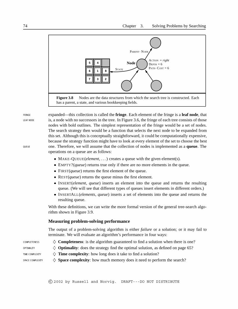
There are many ways to represent nodes, but we will assume a node is a data structurewith five components:
� STATE: the state in the state space to which the node corresponds.
� PARENT-NODE: the node in the search tree that generated this node.
� ACTION: the action that was applied to the parent to generate the node.
� PATH-COST: the cost of the path from the initial state to the node, as indicated by theparent pointers. The path cost is traditionally denoted by ���.
� DEPTH: the number of steps along the path from the initial state.
� In general, we may have a search graph rather than a search tree, when the same state can be reached frommultiple paths. We defer consideration of this complication until Section 3.5.
c� 2002 by Russell and Norvig. DRAFT---DO NOT DISTRIBUTE

Section 3.3. Searching for Solutions 73
It is important to remember the distinction between nodes and states. A node is a bookkeepingdata structure used to represent the search tree. A state corresponds to a configuration of theworld. Thus, nodes are on particular paths, as defined by PARENT-NODE pointers, whereasstates are not. Furthermore, two different nodes can contain the same world state, if that stateis generated via two different search paths. The node data structure is depicted in Figure 3.8.
We also need to represent the collection of nodes that have been generated but not yet
(a) The initial state
(b) After expanding Arad
(c) After expanding Sibiu
Rimnicu Vilcea LugojArad Fagaras Oradea AradArad Oradea
Rimnicu Vilcea Lugoj
ZerindSibiu
Arad Fagaras Oradea
Timisoara
AradArad Oradea
Lugoj AradArad Oradea
Zerind
Arad
Sibiu Timisoara
Arad
Rimnicu Vilcea
Zerind
Arad
Sibiu
Arad Fagaras Oradea
Timisoara
Figure 3.6 Partial search trees for route finding from Arad to Bucharest. Nodes that havebeen expanded are shaded; nodes that have been generated but not yet expanded are outlinedin bold; nodes that have not yet been generated are shown in faint dashed lines.
function TREE-SEARCH( problem, strategy) returns a solution, or failureinitialize the search tree using the initial state of problemloop do
if there are no candidates for expansion then return failurechoose a leaf node for expansion according to strategyif the node contains a goal state then return the corresponding solutionelse expand the node and add the resulting nodes to the search tree
end
Figure 3.7 An informal description of the general tree-search algorithm.
c� 2002 by Russell and Norvig. DRAFT---DO NOT DISTRIBUTE
74 Chapter 3. Solving Problems by Searching
1
23
45
6
7
81
23
45
6
7
8
Node
PARENT− NODE
STATE P COSTATH− = 6DEPTH = 6ACTION = right
Figure 3.8 Nodes are the data structures from which the search tree is constructed. Eachhas a parent, a state, and various bookkeeping fields.
expanded—this collection is called the fringe. Each element of the fringe is a leaf node, thatFRINGE
LEAF NODE is, a node with no successors in the tree. In Figure 3.6, the fringe of each tree consists of thosenodes with bold outlines. The simplest representation of the fringe would be a set of nodes.The search strategy then would be a function that selects the next node to be expanded fromthis set. Although this is conceptually straightforward, it could be computationally expensive,because the strategy function might have to look at every element of the set to choose the bestone. Therefore, we will assume that the collection of nodes is implemented as a queue. TheQUEUE
operations on a queue are as follows:
� MAKE-QUEUE(element, . . . ) creates a queue with the given element(s).
� EMPTY?(queue) returns true only if there are no more elements in the queue.
� FIRST(queue) returns the first element of the queue.
� REST(queue) returns the queue minus the first element.
� INSERT(element, queue) inserts an element into the queue and returns the resultingqueue. (We will see that different types of queues insert elements in different orders.)
� INSERTALL(elements, queue) inserts a set of elements into the queue and returns theresulting queue.
With these definitions, we can write the more formal version of the general tree-search algo-rithm shown in Figure 3.9.
Measuring problem-solving performance
The output of a problem-solving algorithm is either failure or a solution; or it may fail toterminate. We will evaluate an algorithm’s performance in four ways:
� Completeness: is the algorithm guaranteed to find a solution when there is one?COMPLETENESS
� Optimality: does the strategy find the optimal solution, as defined on page 65?OPTIMALITY
� Time complexity: how long does it take to find a solution?TIME COMPLEXITY
� Space complexity: how much memory does it need to perform the search?SPACE COMPLEXITY
c� 2002 by Russell and Norvig. DRAFT---DO NOT DISTRIBUTE

Section 3.3. Searching for Solutions 75
function TREE-SEARCH( problem, fringe) returns a solution, or failure
fringe� INSERT(MAKE-NODE(INITIAL-STATE[problem]), fringe)loop do
if EMPTY?( fringe) then return failurenode�REMOVE-FRONT(fringe)if GOAL-TEST[problem] applied to STATE(node) succeeds
then return SOLUTION(node)fringe� INSERTALL(EXPAND(node, problem), fringe)
end
function EXPAND( node, problem) returns a set of nodes
successors� the empty setfor each �action, result� in SUCCESSOR-FN[problem](STATE[node]) do
successor� a new NODE
STATE[successor]� resultPARENT-NODE[successor]� nodeACTION[successor]� actionPATH-COST[successor]� PATH-COST[node] + STEP-COST(node, action, successor)DEPTH[successor]�DEPTH[node] + 1add successor to successors
endreturn successors
end
Figure 3.9 The general tree-search algorithm. (Note that the fringe argument must be anempty queue, and the type of the queue will affect the order of the search.) The SOLUTION
function returns the sequence of actions obtained by following parent pointers back to theroot.
Time and space complexity are always considered with respect to some measure of the prob-lem difficulty. In theoretical computer science, the typical measure is the size of the statespace graph, because the graph is typically viewed as an explicit data structure that is inputto the search program. (The map of Romania is an example of this.) In AI, where the graphis often represented implicitly by the initial state and successor function and is frequentlyinfinite, complexity is expressed using the following quantities:
� �, the branching factor—the maximum number of successors of any node;BRANCHING FACTOR
� �, the depth of the shallowest goal node;
� �, the maximum length of any path in the state space.
c� 2002 by Russell and Norvig. DRAFT---DO NOT DISTRIBUTE

76 Chapter 3. Solving Problems by Searching
Time is often measured in terms of the number of nodes generated7 during the search, andspace in terms of the maximum number of nodes stored in memory.
To assess the effectiveness of a search algorithm, we can consider just the search cost—SEARCH COST
which typically depends on the time complexity but can also include a term for memoryusage—or we can use the total cost, which combines the search cost and the path cost of theTOTAL COST
solution found. For the problem of finding a route from Arad to Bucharest, the search costis the amount of time taken by the search and the solution cost is the total length of the pathin kilometers. Thus, to compute the total cost, we have to add kilometers and milliseconds.There is no “official exchange rate” between the two, but it might be reasonable in this caseto convert kilometers into milliseconds using an estimate of the car’s average speed (becausetime is what the agent cares about). This enables the agent to find an optimal tradeoff pointat which further computation to find a shorter path becomes counterproductive. The moregeneral problem of tradeoffs between different goods will be taken up in Chapter 16.
3.4 UNINFORMED SEARCH STRATEGIES
This section covers five search strategies that come under the heading of uninformed searchUNINFORMEDSEARCH
(also called blind search). The term means that they have no additional information aboutstates beyond that provided in the problem definition. All they can do is generate successorsand distinguish a goal state from a non-goal state. Strategies that know whether one non-goal state is “more promising” than another are called informed search or heuristic searchINFORMED SEARCH
HEURISTIC SEARCH strategies; they will be covered in Chapter 4. All search strategies are distinguished by theorder in which nodes are expanded.
Breadth-first search
Breadth-first search is a simple strategy in which the root node is expanded first, then all theBREADTH-FIRSTSEARCH
successors of the root node are expanded next, then their successors, and so on. In general,all the nodes are expanded at a given depth in the search tree before any nodes at the nextlevel.
Breadth-first search can be implemented by calling TREE-SEARCH with an emptyfringe that is a first-in-first-out (FIFO) queue, assuring that the nodes that are visited firstwill be expanded first. In other words, calling TREE-SEARCH( problem,FIFO-QUEUE()) re-sults in a breadth-first search. The FIFO queue puts all newly generated successors at the endof the queue, which means that shallow nodes are expanded before deeper nodes. Figure 3.10shows the progress of the search on a simple binary tree.
Let us now evaluate breadth-first search using the four criteria given in the previous sec-tion. We can easily see that it is complete—if the shallowest goal node is at some finite depth�, breadth-first search will eventually find it after expanding all shallower nodes (provided
� Some texts measure time in terms of the number of node expansions instead. The two measures differ by atmost a factor of �. It seems to us that the execution time of a node expansion increases with the number of nodesgenerated in that expansion; moreover, space is consumed by nodes as they are generated.
c� 2002 by Russell and Norvig. DRAFT---DO NOT DISTRIBUTE

Section 3.4. Uninformed Search Strategies 77
the branching factor � is finite). The shallowest goal node is not necessarily the optimal one;technically, breadth-first search is optimal if the path cost is a nondecreasing function of thedepth of the node. (This condition is usually satisfied only when all actions have the samecost.)
So far, the news about breadth-first search has been good. To see why it is not always thestrategy of choice, we have to consider the amount of time and memory it takes to complete asearch. To do this, we consider a hypothetical state space where every state has � successors.The root of the search tree generates � nodes at the first level, each of which generates � morenodes, for a total of �� at the second level. Each of these generates � more nodes, yielding ��
nodes at the third level, and so on. Now suppose that the solution is at depth �. In the worstcase, we would expand all but the last node at level � (since the goal itself is not expanded),generating ����� � nodes at level ���. Then the total number of nodes generated would be
� � �� � �� � � �� � ����� � �� � �������
Every node that is generated must remain in memory, because it is either part of the fringeor is an ancestor of a fringe node. The space complexity is, therefore, the same as the timecomplexity (plus one node for the root).
Those who do complexity analysis are worried (or excited, if they like a challenge) byexponential complexity bounds such as �������. Figure 3.11 shows why. It lists the time andmemory required for a breadth-first search with branching factor � � �, for various valuesof the solution depth �. The table assumes that 10,000 nodes can be generated per second andthat a node requires 1000 bytes of storage. Many search problems fit roughly within theseassumptions (give or take a factor of 100) when run on a modern personal computer.
There are two lessons to be learned from Figure 3.11. First, the memory requirementsare a bigger problem for breadth-first search than the execution time. 31 hours would not betoo long to wait for the solution to an important problem of depth 8, but few computers havethe terabyte of main memory it would take. Fortunately, there are other search strategies thatrequire less memory.
The second lesson is that the time requirements are still a major factor. If your problemhas a solution at depth 12, then (given our assumptions) it will take 35 years for breadth-firstsearch (or indeed any uninformed search) to find it. In general, exponential complexity searchproblems cannot be solved by uninformed methods for any but the smallest instances.
A
B C
D E F G
A
B C
D E F G
A
B C
D E F G
A
B C
D E F G
Figure 3.10 Breadth-first search on a simple binary tree. At each stage, the node to beexpanded next is indicated by a marker.
c� 2002 by Russell and Norvig. DRAFT---DO NOT DISTRIBUTE

78 Chapter 3. Solving Problems by Searching
Uniform-cost search
Breadth-first search is optimal when all step costs are equal, because it always expands theshallowest unexpanded node. By a simple extension, we can find an algorithm that is optimalwith any step cost function. Instead of expanding the shallowest node, uniform-cost searchUNIFORM-COST
SEARCH
expands the node � with the lowest path cost, ���. Note that if all step costs are equal, thisis identical to breadth-first search.
Uniform-cost search does not care about the number of steps a path has, but only abouttheir total cost. Therefore, it will get stuck in an infinite loop if it ever expands a node thathas a zero-cost action leading back to the same state (for example, a ���� action). We canguarantee completeness provided the cost of every step is greater than or equal to some smallpositive constant �. This condition is also sufficient to ensure optimality. It means that thecost of a path always increases as we go along the path. From this property, it is easy tosee that the algorithm expands nodes in order of increasing ���. Therefore, the first goalnode selected for expansion is the optimal solution. (Remember that TREE-SEARCH appliesthe goal test only to the a nodes that are selected for expansion.) We recommend trying thealgorithm out to find the shortest path to Bucharest.
Uniform-cost search is guided by path costs rather than depths, so its complexity cannoteasily be characterized in terms of � and �. Instead, let �� be the cost of the optimal solution,and assume that every action costs at least �. Then the algorithm’s worst-case time and spacecomplexity is �����
�����, which can be much greater than ��. This is because uniform-costsearch can, and often does, explore large trees of small steps before exploring paths involvinglarge and perhaps useful steps. When all step costs are equal, of course, ���
���� is just ��.
Depth-first search
Depth-first search always expands the deepest node in the current fringe of the search tree.DEPTH-FIRSTSEARCH
The progress of the search is illustrated in Figure 3.12. The search proceeds immediatelyto the deepest level of the search tree, where the nodes have no successors. As those nodesare expanded, they are dropped from the fringe, so then the search “backs up” to the nextshallowest node that still has unexplored successors.
This strategy can be implemented by TREE-SEARCH with a last-in-first-out (LIFO)
Depth Nodes Time Memory
2 1100 .11 seconds 1 megabyte4 111,100 11 seconds 106 megabytes6 �� 19 minutes 10 gigabytes8 � 31 hours 1 terabytes
10 ��� 129 days 101 terabytes12 ��� 35 years 10 petabytes14 ��� 3,523 years 1 exabyte
Figure 3.11 Time and memory requirements for breadth-first search. The numbers shownassume branching factor � � ��; 10,000 nodes/second; 1000 bytes/node.
c� 2002 by Russell and Norvig. DRAFT---DO NOT DISTRIBUTE

Section 3.4. Uninformed Search Strategies 79
queue, also known as a stack. As an alternative to the TREE-SEARCH implementation, it iscommon to implement depth-first search with a recursive function that calls itself on each ofits children in turn. (A recursive depth-first algorithm incorporating a depth limit is shown inFigure 3.13.)
Depth-first search has very modest memory requirements. It needs to store only a singlepath from the root to a leaf node, along with the remaining unexpanded sibling nodes for eachnode on the path. Once a node has been expanded, it can be removed from memory as soonas all its descendants have been fully explored (see Figure 3.12). For a state space withbranching factor � and maximum depth �, depth-first search requires storage of only ����nodes. Using the same assumptions as Figure 3.11, and assuming that nodes at the samedepth as the goal node have no successors, we find that depth-first search would require 118kilobytes instead of 10 petabytes at depth � � ��, a factor of 10 billion times less space.
A variant of depth-first search called backtracking search uses still less memory. InBACKTRACKINGSEARCH
backtracking, only one successor is generated at a time rather than all successors; each par-
A
B C
D E F G
H I J K L M N O
A
B C
D E F G
H I J K L M N O
A
B C
D E F G
H I J K L M N O
A
B C
D E F G
H I J K L M N O
A
B C
D E F G
H I J K L M N O
A
B C
D E F G
H I J K L M N O
A
B C
D E F G
H I J K L M N O
A
B C
D E F G
H I J K L M N O
A
B C
D E F G
H I J K L M N O
A
B C
D E F G
H I J K L M N O
A
B C
D E F G
H I J K L M N O
A
B C
D E F G
H I J K L M N O
Figure 3.12 Depth-first search on a binary tree. Nodes that have been expanded and haveno descendants in the fringe can be removed from memory; these are shown in black. Nodesat depth 3 are assumed to have no successors and � is the only goal node.
c� 2002 by Russell and Norvig. DRAFT---DO NOT DISTRIBUTE

80 Chapter 3. Solving Problems by Searching
tially expanded node remembers which successor to generate next. In this way, only ����memory is needed rather than �����. Backtracking search facilitates yet another memory-saving (and time-saving) trick: the idea of generating a successor by modifying the currentstate description directly rather than copying it first. This reduces the memory requirementsto just one state description and ���� actions. For this to work, we must be able to undoeach modification when we go back to generate the next successor. For problems with largestate descriptions, such as robotic assembly, these techniques are critical to success.
The drawback of depth-first search is that it can make a wrong choice and get stuckgoing down a very long (or even infinite) path when a different choice would lead to a solutionnear the root of the search tree. For example, in Figure 3.12, depth-first search will explorethe entire left subtree even if node � is a goal node. If node � were also a goal node, thendepth-first search would return it as a solution; hence, depth-first search is not optimal. Ifthe left subtree were of unbounded depth but contained no solutions, depth-first search wouldnever terminate; hence, it is not complete. In the worst case, depth-first search will generateall of the ����� nodes in the search tree, where � is the maximum depth of any node. Notethat � can be much larger than � (the depth of the shallowest solution), and is infinite if thetree is unbounded.
Depth-limited search
The problem of unbounded trees can be alleviated by supplying depth-first search with a pre-determined depth limit �. That is, nodes at depth � are treated as if they have no successors.This approach is called depth-limited search. The depth limit solves the infinite-path prob-DEPTH-LIMITED
SEARCH
lem. Unfortunately, it also introduces an additional source of incompleteness if we choose� � �, that is, the shallowest goal is beyond the depth limit. (This is not unlikely when �is unknown.) Depth-limited search will also be nonoptimal if we choose � � �. Its timecomplexity is ����� and its space complexity is �����. Depth-first search can be viewed as aspecial case of depth-limited search with ���.
Sometimes, depth limits can be chosen based on knowledge of the problem. For exam-ple, on the map of Romania there are 20 cities. Therefore, we know that if there is a solution,it must be of length 19 at the longest, so � � �� is a possible choice. But in fact if we studiedthe map carefully, we would discover that any city can be reached from any other city in atmost 9 steps. This number, known as the diameter of the state space, gives us a better depthDIAMETER
limit, which leads to a more efficient depth-limited search. For most problems, however, wewill not know a good depth limit until we have solved the problem.
Depth-limited search can be implemented as a simple modification to the general tree-search algorithm or to the recursive depth-first search algorithm. We show the pseudocode forrecursive depth-limited search in Figure 3.13. Notice that depth-limited search can terminatewith two kinds of failure: the standard failure value indicates no solution; the cutoff valueindicates no solution within the depth limit.
Iterative deepening depth-first search
Iterative deepening search (or iterative deepening depth-first search) is a general strategy,ITERATIVEDEEPENING SEARCH
c� 2002 by Russell and Norvig. DRAFT---DO NOT DISTRIBUTE

Section 3.4. Uninformed Search Strategies 81
function DEPTH-LIMITED-SEARCH( problem, limit) returns a solution, or failure/cutoffreturn RECURSIVE-DLS(MAKE-NODE(INITIAL-STATE[problem]), problem, limit)
function RECURSIVE-DLS(node, problem, limit) returns a solution, or failure/cutoffcutoff-occurred?� falseif GOAL-TEST[problem](STATE[node]) then return SOLUTION(node)else if DEPTH[node] = limit then return cutoffelse for each successor in EXPAND(node, problem) do
result�RECURSIVE-DLS(successor, problem, limit)if result = cutoff then cutoff-occurred?� trueelse if result �� failure then return result
endif cutoff-occurred? then return cutoff else return failure
Figure 3.13 A recursive implementation of depth-limited search.
often used in combination with depth-first search, that finds the best depth limit. It does thisby gradually increasing the limit—first 0, then 1, then 2, and so on—until a goal is found. Thiswill occur when when the depth limit reaches �, the depth of the shallowest goal node. Thealgorithm is shown in Figure 3.14. Iterative deepening combines the benefits of depth-firstand breadth-first search. Like depth-first search, its memory requirements are very modest:����� to be precise. Like breadth-first search, it is complete when the branching factor isfinite and optimal when the path cost is a nondecreasing function of the depth of the node.Figure 3.15 shows four iterations of ITERATIVE-DEEPENING-SEARCH on a binary searchtree, where the solution is found on the fourth iteration.
Iterative deepening search may seem wasteful, because states are generated multipletimes. For most problems, however, the overhead of this repeated generation is actuallyrather small. Intuitively, the reason is that in a search tree with the same (or nearly the same)branching factor at each level, most of the nodes are in the bottom level, so it does not mattermuch that the upper levels are generated multiple times. In an iterative deepening search, the
function ITERATIVE-DEEPENING-SEARCH( problem) returns a solution, or failureinputs: problem, a problem
for depth� 0 to � doresult�DEPTH-LIMITED-SEARCH( problem, depth)if result �� cutoff then return result
end
Figure 3.14 The iterative deepening search algorithm, which repeatedly applies depth-limited search with increasing limits. It terminates when a solution is found or if the depth-limited search returns failure, meaning that no solution exists.
c� 2002 by Russell and Norvig. DRAFT---DO NOT DISTRIBUTE

82 Chapter 3. Solving Problems by Searching
nodes on the bottom level (depth �) are generated once, those on the next to bottom level aregenerated twice, and so on, up to the children of the root, which are generated � times. So thetotal number of node generations in an iterative deepening search is given by
��IDS� � ���� � ��� ���� � � �����
which gives a time complexity of �����. We can compare this to the nodes generated by abreadth-first search:
��BFS� � � � �� � � �� � ����� � ��
Notice that breadth-first search generates some nodes at depth ���, whereas iterative deepen-ing does not. The result is that iterative deepening is actually faster than breadth-first search,
Limit = 3
Limit = 2
Limit = 1
Limit = 0 A A
A
B C
A
B C
A
B C
A
B C
A
B C
D E F G
A
B C
D E F G
A
B C
D E F G
A
B C
D E F G
A
B C
D E F G
A
B C
D E F G
A
B C
D E F G
A
B C
D E F G
A
B C
D E F G
H I J K L M N O
A
B C
D E F G
H I J K L M N O
A
B C
D E F G
H I J K L M N O
A
B C
D E F G
H I J K L M N O
A
B C
D E F G
H I J K L M N O
A
B C
D E F G
H I J K L M N O
A
B C
D E F G
H I J K L M N O
A
B C
D E F G
H I J K L M N O
A
B C
D E F G
H I J K L M N O
A
B C
D E F G
H I J K L M N O
A
B C
D E F G
H J K L M N OI
A
B C
D E F G
H I J K L M N O
Figure 3.15 Four iterations of iterative deepening search on a binary tree.
c� 2002 by Russell and Norvig. DRAFT---DO NOT DISTRIBUTE

Section 3.4. Uninformed Search Strategies 83
GoalStart
Figure 3.16 A schematic view of a bidirectional search that is about to succeed, when abranch from the start node meets a branch from the goal node.
despite the repeated generation of states. For example, if � � � and � � , the numbers are
��IDS� � � � � � � � � � ���
��BFS� � � � � � � � � � � � ��� �� � � ��� �
In general, iterative deepening is the preferred uninformed search method when there is alarge search space and the depth of the solution is not known.
Iterative deepening search is analogous to breadth-first search in that it explores a com-plete layer of new nodes at each iteration before going on to the next layer. It would seemworthwhile to develop an iterative analogue to uniform-cost search, inheriting the latter al-gorithm’s optimality guarantees while avoiding its memory requirements. The idea is to useincreasing path-cost limits instead of increasing depth limits. The resulting algorithm, callediterative lengthening search, is explored in Exercise 3.11. It turns out, unfortunately, that
ITERATIVELENGTHENINGSEARCH
iterative lengthening incurs substantial overhead compared to uniform-cost search.
Bidirectional search
The idea behind bidirectional search is to run two simultaneous searches—one forward fromthe initial state and the other backward from the goal, stopping when the two searches meetin the middle (Figure 3.16). The motivation is that ���� � ���� is much less than ��.
Bidirectional search is implemented by having one or both of the searches check eachnode before it is expanded to see if it is in the fringe of the other search tree; if so, a solutionhas been found. For example, if a problem has solution depth ���, and each direction runsbreadth-first search one node at a time, then in the worst case the two searches meet wheneach has expanded all but one of the nodes at depth 3. For ���, this means a total of 22,200node generations, compared to 11,111,100 for a standard breadth-first search. Checking anode for membership in the other search tree can be done in constant time with a hash table,so the time complexity of bidirectional search is �������. At least one of the search trees mustbe kept in memory so that the membership check can be done, hence the space complexityis also �������. This space requirement is the most significant weakness of bidirectionalsearch. The algorithm is complete and optimal (for uniform step costs) if both searches arebreadth-first; other combinations may sacrifice completeness, optimality, or both.
c� 2002 by Russell and Norvig. DRAFT---DO NOT DISTRIBUTE

84 Chapter 3. Solving Problems by Searching
The reduction in time complexity makes bidirectional search attractive, but how dowe search backwards? This is not as easy as it sounds. Let the predecessors of a node �,PREDECESSORS
�������, be all those nodes that have � as a successor. Bidirectional search requires that������� be efficiently computable. The easiest case is when all the actions in the state spaceare reversible, so that ���������������. Other cases may require substantial ingenuity.
Consider the question of what we mean by “the goal” in searching “backward from thegoal.” For the 8-puzzle and for route finding in Romania, there is just one goal state so thebackward search is very much like the forward search. If there are several explicitly listed goalstates—for example, the two dirt-free goal states in Figure 3.3—then we can construct a newdummy goal state whose immediate predecessors are all the actual goal states. Alternatively,some redundant node generations can be avoided by viewing the set of goal states as a singlestate, each of whose predecessors is also a set of states—specifically, the set of states havinga corresponding successor in the set of goal states (see also Section 3.6).
The most difficult case for bidirectional search is when the goal test gives only an im-plicit description of some possibly large set of goal states—for example, all the states satisfy-ing the “checkmate” goal test in chess. A backward search would need to construct compactdescriptions of “all states that lead to checkmate by move ��” and so on; and those descrip-tions would have to be tested against the states generated by the forward search. There is nogeneral way to do this efficiently.
Comparing uninformed search strategies
Figure 3.17 compares search strategies in terms of the four evaluation criteria set forth inSection 3.4.
CriterionBreadth- Uniform- Depth- Depth- Iterative Bidirectional
First Cost First Limited Deepening (if applicable)
Complete? Yes� Yes��� No No Yes� Yes���
Time ������� ���������� ����� ���� ����� �������
Space ������� ���������� ����� ����� ����� �������
Optimal? Yes Yes No No Yes Yes��
Figure 3.17 Evaluation of search strategies. � is the branching factor; � is the depth ofthe shallowest solution; � is the maximum depth of the search tree; � is the depth limit.Superscript caveats are as follows: � complete if � is finite; � complete if step costs � forpositive ; optimal if step costs are all identical; � if both directions use breadth-first search.
3.5 AVOIDING REPEATED STATES
Up to this point, we have all but ignored one of the most important complications to thesearch process: the possibility of wasting time by expanding states that have already beenencountered and expanded before. For some problems, this possibility never comes up; the
c� 2002 by Russell and Norvig. DRAFT---DO NOT DISTRIBUTE

Section 3.5. Avoiding Repeated States 85
state space is a tree and there is only one path to each state. The efficient formulation of the 8-queens problem (where each new queen is placed in the leftmost empty column) is efficient inlarge part because of this—each state can only be reached through one path. If we formulatethe 8-queens problem so that a queen can be placed in any column, then each state with �queens can be reached by �� different paths.
For some problems, repeated states are unavoidable. This includes all problems wherethe actions are reversible, such as route-finding problems and sliding-blocks puzzles. Thesearch trees for these problems are infinite, but if we prune some of the repeated states, wecan cut the search tree down to finite size, generating only the portion of the tree that spansthe state space graph. Considering just the search tree up to a fixed depth, it is easy tofind cases where eliminating repeated states yields an exponential reduction in search cost.In the extreme case, a state space of size � � � (Figure 3.18(a)) becomes a tree with ��
leaves (Figure 3.18(b)). A more realistic example is the rectangular grid as illustrated inRECTANGULAR GRID
Figure 3.18(c). On a grid, each state has four successors, so the search tree including repeatedstates has � leaves; but there are only about ��� distinct states within � steps of any givenstate. For � � �, this means about a trillion nodes but only about 800 distinct states.
Repeated states, then, can cause a solvable problem to become unsolvable if the al-gorithm does not detect them. Detection usually means comparing the node about to beexpanded to those that have been expanded already; if a match is found, then the algorithmhas discovered two paths to the same state and can discard one of them.
For depth-first search, the only nodes in memory are those on the path from the root tothe current node. Comparing those nodes to the current node allows the algorithm to detectlooping paths that can be discarded immediately. This is fine for ensuring that finite statespaces do not become infinite search trees because of loops; unfortunately, it does not avoidthe exponential proliferation of non-looping paths in problems such as those in Figure 3.18.The only way to avoid these is to keep more nodes in memory. Thus, we have a fundamentaltradeoff between space and time. Algorithms that forget their history are doomed to repeatit.
If an algorithm remembers every state that it has visited, then it can be viewed as ex-ploring the state-space graph directly. We can modify the general TREE-SEARCH algorithmto include a data structure called the closed list that stores every expanded node. (The fringeCLOSED LIST
of unexpanded nodes is sometimes called the open list.) If the current node matches a nodeOPEN LIST
on the closed list, it is discarded instead of being expanded. The new algorithm is calledGRAPH-SEARCH (Figure 3.19). On problems with many repeated states, GRAPH-SEARCH
is much more efficient than TREE-SEARCH. Its worst-case time and space requirements areproportional to the size of the state space. As we have seen, this may be much smaller than�����.
Optimality for graph search is a tricky issue. We said earlier that when a repeated stateis detected, the algorithm has found two paths to the same state. The GRAPH-SEARCH al-gorithm in Figure 3.19 always discards the newly discovered path; obviously, if the newlydiscovered path is shorter than the original one, GRAPH-SEARCH may miss an optimal so-lution. Fortunately, we can show (Exercise 3.12) that this cannot happen when using eitheruniform-cost search or breadth-first search with constant step costs; hence, these two optimal
c� 2002 by Russell and Norvig. DRAFT---DO NOT DISTRIBUTE

86 Chapter 3. Solving Problems by Searching
tree search strategies are also optimal graph search strategies. Iterative deepening search, onthe other hand, uses depth-first expansion and can easily follow a suboptimal path to a nodebefore finding the optimal one. Hence, iterative deepening graph search needs to check if anewly discovered path to a node is better than the original one, and, if so, may need to revisethe depths and path costs of that node’s descendants.
Note that the use of a closed list means that depth-first search and iterative deepeningsearch no longer have linear space requirements. Because the GRAPH-SEARCH algorithmkeeps every node in memory, some searches are infeasible because of memory limitations.
A
B
C
D
A
B
CC
B
CC
A
(c)(b)(a)
Figure 3.18 State spaces that generate an exponentially larger search tree. (a) A statespace in which there are two possible actions leading from A to B, two from B to C, andso on. The state space contains � � � states, where � is the maximum depth. (b) The thecorresponding search tree, which has �� branches corresponding to the �� paths through thespace. (c) A rectangular grid space. States within 2 steps of the initial state (A) are shown ingray.
function GRAPH-SEARCH( problem, fringe) returns a solution, or failure
closed� an empty setfringe� INSERT(MAKE-NODE(INITIAL-STATE[problem]), fringe)loop do
if fringe is empty then return failurenode�REMOVE-FRONT(fringe)if GOAL-TEST[problem](STATE[node]) then return SOLUTION(node)if STATE[node] is not in closed then
add STATE[node] to closedfringe� INSERTALL(EXPAND(node, problem), fringe)
end
Figure 3.19 The general graph-search algorithm. The set closed can be implemented witha hash table to allow efficient checking for repeated states. This algorithm assumes that thefirst path to a state is the cheapest (see text).
c� 2002 by Russell and Norvig. DRAFT---DO NOT DISTRIBUTE

Section 3.6. Searching with Partial Information 87
3.6 SEARCHING WITH PARTIAL INFORMATION
In Section 3.3 we assumed that the environment is fully observable and deterministic, andthat the agent knows what the effects of each action are. Therefore, the agent can calculateexactly which state results from any sequence of actions and always knows which state it isin. Its percepts provide no new information after each action. What happens when knowledgeof the states or actions is incomplete? We find that different types of incompleteness lead tothree distinct problem types:
1. Sensorless problems (also called conformant problems): if the agent has no sensorsat all, then (as far as it knows) it may be in one of several possible initial states, andeach action may therefore lead to one of several possible successor states.
2. Contingency problems: if there is uncertainty about action outcomes, or if the en-vironment is partially observable, then the agent’s percepts provide new informationafter each action. Each possible percept defines a contingency that must be planned for.A problem is called adversarial if the uncertainty is caused by the hostile actions ofanother agent.
3. Exploration problems: when the states and actions of the environment are unknown,the agent must act to discover them. Exploration problems can be viewed as an extremecase of contingency problems. Section 4.5.
As an example, we will use the vacuum world environment. Recall that the state space haseight states, as shown in Figure 3.20. There are three actions—Left, Right, and Suck—and thegoal is to clean up all the dirt (states 7 and 8). If the environment is observable, deterministic,and completely known, then the problem is trivially solvable by any of the algorithms we havedescribed. For example, if the initial state is 5, then the action sequence [Right,Suck] willreach a goal state, 8. The remainder of this section deals with the sensorless and contingencyversions of the problem. Exploration problems are covered in Section 4.5 and adversarialproblems in Chapter 6.
Sensorless Problems
Suppose that the vacuum agent knows all the effects of its actions, but has no sensors at all.Then it knows only that its initial state is one of the set �� � � � � ��. One mightsuppose that the agent’s predicament is hopeless, but in fact it can do quite well. Because itknows what its actions do, it can, for example, calculate that the action Right will cause it tobe in one of the states �� � ��, and the action sequence [Right,Suck] will always end up inone of the states � ��. Finally, the sequence [Right,Suck,Left,Suck] is guaranteed to reachthe goal state 7 no matter what the start state. We say that the agent can coerce the world intoCOERCION
state 7, even when it doesn’t know what state it starts from. To summarize: when the world isnot fully observable, the agent must reason about sets of states that it might get to, rather thansingle states. We call each such set of states a belief state, representing the agent’s currentBELIEF STATE
belief about the possible physical states it might be in. Fully observable environments can be
c� 2002 by Russell and Norvig. DRAFT---DO NOT DISTRIBUTE

88 Chapter 3. Solving Problems by Searching
1 2
3 4
5 6
7 8
Figure 3.20 The eight possible states of the vacuum world.
thought of as a special case in which every belief state is a singleton set containing exactlyone physical state.
To solve sensorless problems, we simply search in the space of belief states rather thanphysical states, using any standard search algorithm. The initial state is a belief state, andeach action maps from a belief state to another belief state. An action is applied to a beliefstate by unioning the results of applying the action to each physical state in the belief state.A path now connects several belief states, and a solution is now a path that leads to a beliefstate, all of whose members are goal states. Figure 3.21 shows the reachable belief state spacefor the deterministic, sensorless vacuum world. There are only 12 reachable belief states, butthe entire belief state space contains every possible set of physical states, i.e., ��� � beliefstates. In general, if the physical state space has � states, the belief state space has �� beliefstates.
Our discussion of sensorless problems so far has assumed deterministic actions, but theanalysis is essentially unchanged if the environment is nondeterministic—that is, if actionsmay have several possible outcomes. The reason is that, in the absence of sensors, the agenthas no way to tell which outcome actually occurred, so the various possible outcomes arejust additional physical states in the successor belief state. For example, suppose the theenvironment obeys Murphy’s Law: the so-called Suck action sometimes deposits dirt on thecarpet but only if there is no dirt there already.8 Then, if ���� is applied in physical state4 (see Figure 3.20), there are two possible outcomes: states 2 and 4. Applied to the initialbelief state, �� � � � � ��, ���� now leads to the belief state that is the union of theoutcome sets for the eight physical states. Calculating this, we find that the new belief state is�� � � � � ��. So, for a sensorless agent in the Murphy’s Law world, the ���� actionleaves the belief state unchanged! In fact, the problem is unsolvable (see Exercise 3.18).
� We assume that most readers face similar problems, and can imagine themselves as frustrated as our agent. Weapologize to owners of modern, efficient home appliances who cannot take advantage of this pedagogical device.
c� 2002 by Russell and Norvig. DRAFT---DO NOT DISTRIBUTE

Section 3.6. Searching with Partial Information 89
L
R
L R
S
L RS S
S S
R
L
S S
L
R
R
L
R
L
Figure 3.21 The reachable portion of the belief state space for the deterministic, sensor-less vacuum world. Each dashed-line box encloses a belief state. At any given point, theagent is in a particular belief state but does not know which physical state it is in. The initialbelief state (complete ignorance) is the top center box. Actions are represented by labelledarcs. Self-loops are omitted for clarity.
Intuitively, the reason is that the agent cannot tell if the current square is dirty, and hencecannot tell if the ���� action will clean it up or create more dirt.
Contingency Problems
When the environment is such that the agent can obtain new information from its sensorsafter acting, the agent faces a contingency problems. The solution to a contingency problemCONTINGENCY
PROBLEM
often takes the form of a tree, where each branch may be selected depending on the perceptsreceived up to that point in the tree. For example, suppose that the agent is in the Murphy’sLaw world, and that it has a position sensor and a local dirt sensor, but no sensor capable of
c� 2002 by Russell and Norvig. DRAFT---DO NOT DISTRIBUTE

90 Chapter 3. Solving Problems by Searching
detecting dirt in other squares. Thus, the percept ��� �!� means that the agent is in one ofthe states �� ��. The agent might formulate the action sequence [Suck,Right,Suck]. Suckingwould change the state to one of � ��, and moving right would then change the state to oneof �� ��. Executing the final Suck action in state 6 takes us to state 8, a goal, but executing itin state 8 might take us back to state 6 (by Murphy’s Law), in which case the plan fails.
By examining the belief state space for this version of the problem, it can easily bedetermined that no fixed action sequence guarantees a solution to this problem. There is,however, a solution if we don’t insist on a fixed action sequence:
�Suck Right if [R,Dirty] then Suck� "
This extends the space of solutions to include the possibility of selecting actions based oncontingencies arising during execution. Many problems in the real, physical world are con-tingency problems, because exact prediction is impossible. For this reason, many people keeptheir eyes open while walking around or driving.
Contingency problems sometimes allow purely sequential solutions. For example, con-sider a fully observable Murphy’s Law world. Contingencies arise if the agent performs a���� action in a clean square, because dirt may or may not be deposited in the square. Aslong as the agent never does this, no contingencies arise and there is a sequential solutionfrom every initial state (Exercise 3.18).
The algorithms for contingency problems are more complex than the standard searchalgorithms in this chapter; they are covered in Chapter 12. Contingency problems also lendthemselves to a somewhat different agent design, in which the agent can act before it hasfound a guaranteed plan. This is useful because rather than considering in advance everypossible contingency that might arise during execution, it is often better to start acting andsee which contingencies do arise. The agent can then continue to solve the problem given theadditional information. This type of interleaving of search and execution is also useful forINTERLEAVING
exploration problems (see Section 4.5) and for game playing (see Chapter 6).
3.7 SUMMARY
This chapter has introduced methods that an agent can use to select actions in environmentsthat are deterministic, observable, static, and completely known. In such cases, the agent canconstruct sequences of actions that achieve its goals; this process is called search.
� Before an agent can start searching for solutions, it must formulate a goal and then usethe goal to formulate a problem.
� A problem consists of four parts: the initial state, a set of actions, a goal test function,and a path cost function. The environment of the problem is represented by a statespace. A path through the state space from the initial state to a goal state is a solution.
� In real life, most problems are ill-defined; but with some analysis, many problems canfit into the state space model.
� A single, general TREE-SEARCH algorithm can be used to solve any problem; specificvariants of the algorithm embody different strategies.
c� 2002 by Russell and Norvig. DRAFT---DO NOT DISTRIBUTE

Section 3.7. Summary 91
� Search algorithms are judged on the basis of completeness, optimality, time complex-ity, and space complexity. Complexity depends on �, the branching factor in the statespace, and �, the depth of the shallowest solution.
� Breadth-first search selects the shallowest unexpanded node in the search tree forexpansion. It is complete, optimal for unit step costs, and has time and space complexityof �����. The space complexity makes it impractical in most cases. Uniform-costsearch is similar to breadth-first search but expands the node with lowest path cost, ���. It is complete and optimal provided step costs exceed some positive bound �.
� Depth-first search selects the deepest unexpanded node in the search tree for expan-sion. It is neither complete nor optimal, and has time complexity of ����� and spacecomplexity of �����, where � is the maximum depth of any path in the state space.
� Depth-limited search imposes a fixed depth limit on a depth-first search.
� Iterative deepening search calls depth-limited search with increasing limits until agoal is found. It is complete, optimal for unit step costs, and has time complexity of����� and space complexity of �����.
� Bidirectional search can enormously reduce time complexity, but is not always appli-cable and may be impractical because of its space complexity.
� When the state space is a graph rather than a tree, it can pay off to check for repeatedstates in the search tree. The GRAPH-SEARCH algorithm eliminates all duplicate states.
� When the environment is partially observable, the agent can apply search algorithms inthe space of belief states, or sets of possible states that the agent might be in. In somecases, a single solution sequence can be constructed; in other cases, a contingency planis required.
BIBLIOGRAPHICAL AND HISTORICAL NOTES
Most of the state-space search problems analyzed in this chapter have a long history in theliterature, and are less trivial than they may seem. The missionaries and cannibals prob-lem used in Exercise 3.9 was analyzed in detail by Amarel (1968). It had been consideredearlier in AI by Simon and Newell (1961), and in operations research by Bellman and Drey-fus (1962). Studies such as these and Newell and Simon’s work on the Logic Theorist (1957)and GPS (1961) led to the establishment of search algorithms as the primary tools in thearmory of 1960s AI researchers, and the establishment of problem solving as the canoni-cal AI task. A more recent treatment of problem representation and abstraction, includingAI programs that themselves perform these tasks (in part), is in Knoblock (1990).
The 8-puzzle is a smaller cousin of the 15-puzzle, which was invented by the famousAmerican game designer Sam Loyd (1959) in the 1870s. It quickly achieved immense pop-ularity in the United States, comparable to the more recent sensation caused by Rubik’sCube. It also quickly attracted the attention of mathematicians (Johnson and Story, 1879;Tait, 1880). The editors of the American Journal of Mathematics stated “The ‘15’ puzzlefor the last few weeks has been prominently before the American public, and may safely be
c� 2002 by Russell and Norvig. DRAFT---DO NOT DISTRIBUTE

92 Chapter 3. Solving Problems by Searching
said to have engaged the attention of nine out of ten persons of both sexes and all ages andconditions of the community. But this would not have weighed with the editors to inducethem to insert articles upon such a subject in the American Journal of Mathematics, but forthe fact that " " "” (there follows a summary of the mathematical interest of the 15-puzzle). Anexhaustive analysis of the 8-puzzle was carried out with computer aid by Schofield (1967).Ratner and Warmuth (1986) showed that the general �� � version of the 15-puzzle belongsto the class of NP-complete problems.
The 8-queens problem was first published anonymously in the German chess maga-zine Schach in 1848; it was later attributed to one Max Bezzel. It was republished in 1850,and at that time drew the attention of the eminent mathematician Carl Friedrich Gauss, whoattempted to enumerate all possible solutions, but found only 72. Nauck published all 92solutions later in 1850. Netto (1901) generalized the problem to “�-queens,” and Abramsonand Yung (1989) found an ���� algorithm.
Each of the real-world search problems listed in the chapter has been the subject of agood deal of research effort. Methods for selecting optimal airline flights remain proprietaryfor the most part, but Carl de Marcken (personal communication) has shown that airline ticketpricing and restrictions have become so convoluted that the problem of selecting an optimalflight is formally undecidable. The travelling salesperson problem is a standard combina-torial problem in theoretical computer science (Lawler, 1985; Lawler et al., 1992). Karp(1972) proved the TSP to be NP-hard, but effective heuristic approximation methods weredeveloped (Lin and Kernighan, 1973). Arora (1998) devised a fully polynomial approxi-mation scheme for Euclidean TSPs. VLSI layout methods are surveyed by Shahookar andMazumder (1991) and many layout optimization papers appear in VLSI journals. Roboticnavigation and assembly problems are discussed in Chapter 25.
Uninformed search algorithms for problem solving are a central topic of classical com-puter science (Horowitz and Sahni, 1978) and operations research (Dreyfus, 1969); Deo andPang (1984) and Gallo and Pallottino (1988) give more recent surveys. Breadth-first searchwas formulated for solving mazes by Moore (1959). The method of dynamic program-ming (Bellman and Dreyfus, 1962), which systematically records solutions for all subprob-lems of increasing lengths, can be seen as a form of breadth-first search on graphs. Thetwo-point shortest path algorithm of Dijkstra (1959) is the origin of uniform-cost search.
A version of iterative deepening designed to make efficient use of the chess clock wasfirst used by Slate and Atkin (1977) in the CHESS 4.5 game-playing program, but the appli-cation to shortest path graph search is due to Korf (1985a). Iterative broadening (GinsbergITERATIVE
BROADENING
and Harvey, 1992) is a complementary technique in which each iteration of the search mayexpand at most � successors of each node; � is increased on each iteration to ensure com-pleteness. This technique is sometimes useful for problems with large branching factors.Bidirectional search, which was introduced by Pohl (1969, 1971), can also be very effectivein some cases.
Partially observable and nondeterministic environments have not been studied in greatdepth within the problem-solving approach. Some efficiency issues in belief-state searchhave been investigated by Genesereth and Nourbakhsh (1993). Koenig and Simmons (1998)studied robot navigation from an unknown initial position, and Erdmann and Mason (1988)
c� 2002 by Russell and Norvig. DRAFT---DO NOT DISTRIBUTE

Section 3.7. Summary 93
studied the problem of robotic manipulation without sensors, using a continuous form ofbelief-state search. Contingency search has been studied within the planning subfield (seeChapter 12). For the most part, planning and acting with uncertain information have beenhandled using the tools of probability and decision theory (see Chapter 17).
The textbooks by Nilsson (1971, 1980) are good general sources of information aboutclassical search algorithms. A comprehensive and more up-to-date survey can be foundin (Korf, 1988). Papers about new search algorithms—which, remarkably, continue to bediscovered—appear in journals such as Artificial Intelligence.
EXERCISES
3.1 Define in your own words the following terms: state, state space, search tree, searchnode, goal, action, successor function, and branching factor.
3.2 Explain why problem formulation must follow goal formulation.
3.3 Suppose that LEGAL-ACTIONS�#� denotes the set of actions that are legal in state #,and RESULT�� #� denotes the state that results from performing a legal action � in state #.Explain how to define SUCCESSOR-FN in terms of LEGAL-ACTIONS and RESULT, and viceversa.
3.4 Show that the 8-puzzle states are divided into two disjoint sets, such that no state inone set can be transformed into a state in the other set by any number of moves. [Hint: seeBerlekamp et al. (1982).] Devise a recognition procedure that will tell you if a given state isin one class or the other, and explain why this is a good thing to have for generating randomstarting positions.
3.5 Consider the �-queens problem using the “efficient” incremental formulation given onpage 70. Explain why the state space size is at least �
�� and estimate the largest � for
which exhaustive exploration is feasible. [Hint: Derive a lower bound on the branchingfactor by considering the maximum number of squares that a queen can attack in any givencolumn.]
3.6 Does a finite state space always lead to a finite search tree? How about a finite statespace that is a tree? Can you be more precise about what types of state spaces always lead tofinite search trees? (Adapted from Bender, 1996.)
3.7 Give the initial state, goal test, successor function, and cost function for each of thefollowing. Choose a formulation that is precise enough to be implemented.
a. You have to color a planar map using only four colors, with no two adjacent regionshaving the same color.
b. A 3-foot-tall monkey is in a room where some bananas are suspended from the 8-footceiling. He would like to get the bananas. The room contains two stackable, movable,climbable 3-foot high crates.
c� 2002 by Russell and Norvig. DRAFT---DO NOT DISTRIBUTE

94 Chapter 3. Solving Problems by Searching
c. You have a program that outputs the message “illegal input record” when fed a file ofinput records. You know that processing of each record is independent of the otherrecords. You want to determine what record is illegal.
d. You have three jugs measuring 12 gallons, 8 gallons, and 3 gallons, and a water faucet.You can fill the jugs up, or empty them out from one to another or onto the ground. Youneed to measure out exactly one gallon.
3.8 Consider a state space where the start state is number 1, and the successor function forstate � returns two states labelled �� and �� � �.
a. Draw the portion of the state space for states 1 to 15.
b. Suppose that the goal state is 11. List the order in which nodes will be visited forbreadth-first search, depth-limited search with depth limit 3, and iterative deepeningsearch.
c. Would bidirectional search be appropriate for this problem? If so, describe how it wouldwork. What is the branching factor in each direction of the bidirectional search? Doesthis suggest a reformulation of the problem that would allow you to solve the problemof getting from state 1 to a given goal state with almost no search at all?
3.9 The missionaries and cannibals problem is usually stated as follows. Three mission-aries and three cannibals are on one side of a river, along with a boat that can hold one or twopeople. Find a way to get everyone to the other side, without ever leaving a group of mis-sionaries in one place outnumbered by the cannibals in that place. This problem is famous inAI because it was the subject of the first paper that approached problem formulation from ananalytical viewpoint (Amarel, 1968).
a. Formulate the problem precisely, making only those distinctions necessary to ensure avalid solution. Draw a diagram of the complete state space.
b. Implement and solve the problem optimally using an appropriate search algorithm. Is ita good idea to check for repeated states? decide.
c. Why do you think people have a hard time with this puzzle, when the state space is sosimple?
3.10 Implement two versions of the successor function for the 8-puzzle: one that generatesall the successors at once by copying and editing the 8-puzzle data structure, and one thatgenerates one new successor each time it is called and works by modifying the parent statedirectly (and undoing the modifications as needed). Write versions of iterative deepeningdepth-first search that use these functions and compare their performance.
3.11 On page 83, we mentioned iterative lengthening search, an iterative analogue ofuniform-cost search. The basic idea is to use increasing limits on path cost. If a node isgenerated whose path cost exceeds the current limit, it is immediately discarded. For eachnew iteration, the limit is set to the lowest path cost of any node discarded in the previousiteration.
a. Show that this algorithm is optimal for general path costs.
c� 2002 by Russell and Norvig. DRAFT---DO NOT DISTRIBUTE

Section 3.7. Summary 95
b. Consider a uniform tree with branching factor �, solution depth �, and unit step costs.How many iterations will iterative lengthening require?
c. Now consider step costs drawn from the continuous range � �� with a minimum cost�. How many iterations are required in the worst case?
d. Implement the algorithm and apply it to instances of the 8-puzzle and travelling sales-person problems. Compare the algorithm’s performance to that of uniform-cost search,and comment on your results.
3.12 Prove that uniform-cost search and breadth-first search with constant step costs are op-timal when used with the GRAPH-SEARCH algorithm. Show a state space with constant stepcosts in which GRAPH-SEARCH using iterative deepening finds a suboptimal solution.
3.13 Describe a state space in which iterative deepening search performs much worse thandepth-first search (for example, ����� vs. ����).
3.14 Write a program that will take as input two web page URLs and find a path of linksfrom one to the other. What is an appropriate search strategy? Is bidirectional search a goodidea? Could a search engine be used to implement a predecessor function?
3.15 Consider the problem of finding the shortest path between two points on a plane thathas convex polygonal obstacles as shown in Figure 3.22. This is an idealization of the problemthat a robot has to solve to navigate its way around a crowded environment.
a. Suppose the state space consists of all positions �� � in the plane. How many statesare there? How many paths are there to the goal?
b. Explain briefly why the shortest path from one polygon vertex to any other in the scenemust consist of straight-line segments joining some of the vertices of the polygons.Define a good state space now. How large is this state space?
c. Define the necessary functions to implement the search problem, including a successorfunction that takes a vertex as input and returns the set of vertices that can be reached ina straight line from the given vertex. (Do not forget the neighbors on the same polygon.)Use the straight-line distance for the heuristic function.
d. Apply one or more of the algorithms in this chapter to solve a range of problems in thedomain, and comment on their performance.
3.16 We can turn the navigation problem in Exercise 3.15 into a complete environment asfollows:
� The percept will be a list of the positions, relative to the agent, of the visible vertices.The percept does not include the position of the robot! The robot must determine itsown position from the map; for now, you can assume that each location has a different“view.”
� Each action will be a vector describing a straight-line path to follow. If the path isunobstructed, the action succeeds; otherwise, the robot stops at the point where its pathfirst intersects an obstacle. If the agent returns a zero motion vector and is at the goal(which is fixed and known), then the environment should teleport the agent to a randomlocation (not inside an obstacle).
c� 2002 by Russell and Norvig. DRAFT---DO NOT DISTRIBUTE

96 Chapter 3. Solving Problems by Searching
Figure 3.22 A scene with polygonal obstacles.
� The performance measure charges the agent 1 point for each unit of distance traversedand awards 1000 points each time the goal is reached.
a. Implement this environment and a problem-solving agent for it. The agent will needto formulate a new problem after each teleportation, which will involve determining itscurrent location.
b. Demonstrate your agent working (by having the agent generate suitable commentary asit moves around) and determine its performance over 100 episodes.
c. Modify the environment so that 30% of the time the agent ends up at an unintendeddestination (chosen randomly from the other visible vertices if any, otherwise no moveat all). This is a crude model of the motion errors of a real robot. Modify the agentso that when such an error is detected, it finds out where it is and then constructs aplan to get back to where it was and resume the old plan. Remember that sometimesgetting back to where it was may fail also! Show an example of the agent successfullyovercoming two successive motion errors and still reaching the goal.
d. Now try two different recovery schemes after an error: (1) head for the closest vertex onthe original route; and (2) replan a route to the goal from the new location. Compare theperformance of the three recovery schemes. Would the inclusion of search costs affectthe comparison?
e. Now suppose that there are locations from which the view is identical. (For example,suppose the world is a grid with square obstacles.) What kind of problem does the agentnow face? What do solutions look like?
3.17 On page 65, we said that we would not consider problems with negative path costs. Inthis exercise, we explore this in more depth.
a. Suppose that actions can have arbitrarily large negative costs; explain why this possi-bility would force any optimal algorithm to explore the entire state space.
b. Does it help if we insist that step costs must be greater than or equal to some negativeconstant �? Consider both trees and graphs.
c� 2002 by Russell and Norvig. DRAFT---DO NOT DISTRIBUTE

Section 3.7. Summary 97
c. Suppose that there is a set of operators that form a loop, so that executing the set in someorder results in no net change to the state. If all of these operators have negative cost,what does this imply about the optimal behavior for an agent in such an environment?
d. One can easily imagine operators with high negative cost, even in domains such asroute-finding. For example, some stretches of road might have such beautiful sceneryas to far outweigh the normal costs in terms of time and fuel. Explain, in precise terms,within the context of state-space search, why humans do not drive round scenic loopsindefinitely, and explain how to define the state space and operators for route-finding sothat artificial agents can also avoid looping.
e. Can you think of a real domain in which step costs are such as to cause looping?
3.18 Consider the sensorless, two-location vacuum world under Murphy’s Law. Draw thereachable belief state space given the initial belief state �� � � � � ��, and explainwhy the problem is unsolvable. Show also that if the world is fully observable then there is asolution sequence for each possible initial state.
3.19 Consider the vacuum world problem defined in Figure 2.2.
a. Which of the algorithms defined in this chapter would be appropriate for this problem?Should the algorithm check for repeated states?
b. Apply your chosen algorithm to compute an optimal sequence of actions for a �� �world whose initial state has dirt in the three top squares and the agent in the centersquare.
c. Construct a search agent for the vacuum world, and evaluate its performance in a set of�� � worlds with probability 0.2 of dirt in each square. Include the search cost as wellas path cost in the performance measure, using a reasonable exchange rate.
d. Compare your best search agent with a simple randomized reflex agent that sucks ifthere is dirt, otherwise moves randomly.
e. Consider what would happen if the world was enlarged to �� �. How does the perfor-mance of the search agent and of the reflex agent vary with �?
c� 2002 by Russell and Norvig. DRAFT---DO NOT DISTRIBUTE

4INFORMED SEARCH ANDEXPLORATION
In which we see how information about the state space can prevent algorithmsfrom blundering about in the dark.
Chapter 3 showed that uninformed search strategies can find solutions to problems by system-atically generating new states and testing them against the goal. Unfortunately, these strate-gies are incredibly inefficient in most cases. This chapter shows how an informed searchstrategy—one that uses problem-specific knowledge—can find solutions more efficiently.Section 4.1 describes informed versions of the algorithms in Chapter 3, and Section 4.2 ex-plains how the necessary problem-specific information can be obtained. Sections 4.3 and 4.4cover algorithms that perform purely local search in the state space, evaluating and modify-ing one or more current states rather than systematically exploring paths from an initial state.These algorithms are suitable for problems in which the path cost is irrelevant and all thatmatters is the solution state itself. The family of local-search algorithms includes methodsinspired by statistical physics (simulated annealing) and evolutionary biology (genetic al-gorithms). Finally, Section 4.5 investigates online search, in which the agent is faced with astate space that is completely unknown.
4.1 INFORMED (HEURISTIC) SEARCH STRATEGIES
This section shows how an informed search strategy—one that uses problem-specific knowl-INFORMED SEARCH
edge beyond the definition of the problem itself—can find solutions more efficiently than anuninformed strategy.
The general approach we will consider is called best-first search. Best-first search isBEST-FIRST SEARCH
an instance of the general TREE-SEARCH or GRAPH-SEARCH algorithm in which a node isselected for expansion based on an evaluation function, ����. Traditionally, the node withEVALUATION
FUNCTION
the lowest evaluation is selected for expansion, because the evaluation measures distance tothe goal. Best-first search can be implemented within our general search framework via apriority queue, a data structure that will maintain the fringe in ascending order of � -values.
The name “best-first search” is a venerable but inaccurate one. After all, if we couldreally expand the best node first, it would not be a search at all; it would be a straight march to
98

Section 4.1. Informed (Heuristic) Search Strategies 99
the goal. All we can do is choose the node that appears to be best according to the evaluationfunction. If the evaluation function is exactly accurate, then this will indeed be the bestnode; in reality, the evaluation function will sometimes be off, and can lead the search astray.Nevertheless, we will stick with the name “best-first search,” because “seemingly-best-firstsearch” is a little awkward.
There is a whole family of BEST-FIRST-SEARCH algorithms with different evaluationfunctions.1 A key component of these algorithms is a heuristic function,2 denoted ����:HEURISTIC
FUNCTION
���� � estimated cost of the cheapest path from node n to a goal node.
For example, in Romania, one might estimate the cost of the cheapest path from Arad toBucharest via the straight-line distance from Arad to Bucharest.
Heuristic functions are the most common form in which additional knowledge of theproblem is imparted to the search algorithm. We will study heuristics in more depth in Sec-tion 4.2. For now, we will consider them to be arbitrary problem-specific functions, with oneconstraint: if � is a goal node, then ����� �. The remainder of this section covers two waysto use heuristic information to guide search.
Greedy best-first search
Greedy best-first search3 tries to expand the node that is closest to the goal, on the groundsGREEDY BEST-FIRSTSEARCH
that this is likely to lead to a solution quickly. Thus, it evaluates nodes by using just theheuristic function: ���� � ����.
Let us see how this works for route-finding problems in Romania, using the straight-line distance heuristic, which we will call ����. If the goal is Bucharest, we will need toSTRAIGHT-LINE
DISTANCE
know the straight-line distances to Bucharest, which are shown in Figure 4.1. For example,��������������� ���. Notice that the values of ���� cannot be computed from the prob-lem description itself. Moreover, it takes a certain amount of experience to know that ����is correlated with actual road distances and is, therefore, a useful heuristic.
Urziceni
NeamtOradea
Zerind
Timisoara
Mehadia
Sibiu
PitestiRimnicu Vilcea
Vaslui
241
253329
80199
380234
374
Bucharest
GiurgiuHirsova
Eforie
Arad
Lugoj
DobretaCraiova
Fagaras
Iasi
0160242161
77151
366
244226
176
100193
Figure 4.1 Values of ����—straight-line distances to Bucharest.
� Exercise 4.3 asks you to show that this family includes several familiar uninformed algorithms.� A heuristic function ���� takes a node as input, but is depends only on the state at that node.� Our first edition called this greedy search; other authors have called it best-first search. Our more generalusage of the latter term follows Pearl (1984).
c� 2002 by Russell and Norvig. DRAFT---DO NOT DISTRIBUTE

100 Chapter 4. Informed Search and Exploration
Rimnicu Vilcea
Zerind
Arad
Sibiu
Arad Fagaras Oradea
Timisoara
Sibiu Bucharest
329 374
366 380 193
253 0
Rimnicu Vilcea
Zerind
Arad
Sibiu
Arad Fagaras Oradea
Timisoara
329 374
366 176 380 193
Zerind
Arad
Sibiu Timisoara
253 329 374
Arad
366
(a) The initial state
(b) After expanding Arad
(c) After expanding Sibiu
(d) After expanding Fagaras
Figure 4.2 Stages in a greedy best-first search for Bucharest using the straight-line dis-tance heuristic ����. Nodes are labeled with their �-values.
Figure 4.2 shows the progress of a greedy best-first search using ���� to find a pathfrom Arad to Bucharest. The first node to be expanded from Arad will be Sibiu, because itis closer to Bucharest than either Zerind or Timisoara. The next node to be expanded willbe Fagaras, because it is closest. Fagaras in turn generates Bucharest, which is the goal.For this particular problem, greedy best-first search using ���� finds a solution without everexpanding a node that is not on the solution path; hence, its search cost is minimal. It isnot optimal, however: the path via Sibiu and Fagaras to Bucharest is 32 kilometers longerthan the path through Rimnicu Vilcea and Pitesti. This shows why the algorithm is called“greedy”—it prefers to take the biggest bite possible out of the remaining cost to reach thegoal. It ignores the cost of getting to a node in the first place.
Minimizing ���� is susceptible to false starts. Consider the problem of getting from
c� 2002 by Russell and Norvig. DRAFT---DO NOT DISTRIBUTE

Section 4.1. Informed (Heuristic) Search Strategies 101
Iasi to Fagaras. The heuristic suggests that Neamt be expanded first, because it is closestto Fagaras, but it is a dead end. The solution is to go first to Vaslui—a step that is actuallyfarther from the goal according to the heuristic—and then to continue to Urziceni, Bucharest,and Fagaras. In this case, then, the heuristic causes unnecessary nodes to be expanded. Fur-thermore, if we are not careful to detect repeated states, the solution will never be found—thesearch will oscillate between Neamt and Iasi.
Greedy best-first search resembles depth-first search in the way it prefers to follow asingle path all the way to the goal, but will back up when it hits a dead end. It suffers fromthe same defects as depth-first search—it is not optimal, and it is incomplete (because it canstart down an infinite path and never return to try other possibilities). The worst-case timeand space complexity is ���, where � is the maximum depth of the search space. With agood heuristic function, however, the complexity can be reduced substantially. The amountof the reduction depends on the particular problem and on the quality of the heuristic.
A� search: Minimizing the total estimated solution cost
The most widely-known form of best-first search is called A� search (pronounced “A-starA�
SEARCH
search”). It evaluates nodes by combining ����, the cost to reach the node, and ����, the costto get from the node to the goal:
���� � ���� � ����
Since ���� gives the path cost from the start node to node �, and ���� is the estimated costof the cheapest path from � to the goal, we have
���� � estimated cost of the cheapest solution through �
Thus, if we are trying to find the cheapest solution, a reasonable thing to try first is thenode with the lowest value of ���� � ����. It turns out that this strategy is more than justreasonable: provided that the heuristic function ���� satisfies certain conditions, A� searchis both complete and optimal.
The optimality of A� is very straightforward to analyze when it is used with TREE-SEARCH.In this case, A� is optimal if ���� is an admissible heuristic—that is, provided that ����ADMISSIBLE
HEURISTIC
never overestimates the cost to reach the goal. Admissible heuristics are by nature optimistic,because they think the cost of solving the problem is less than it actually is. Since ���� is theexact cost to reach �, we have as immediate consequence that ���� never overestimates thetrue cost of a solution through �.
An obvious example of an admissible heuristic is the straight-line distance ���� thatwe used in getting to Bucharest. Straight-line distance is admissible because the shortest pathbetween any two points is a straight line, so the straight line cannot be an overestimate. InFigure 4.3, we show the progress of an A� tree search for Bucharest. The values of � arecomputed from the step costs in Figure 3.2, and the values of ���� are given in Figure 4.1.Notice in particular that Bucharest first appears on the fringe at step (e), but it is not selectedfor expansion because its � -cost (450) is higher than that of Pitesti (417). Another way tosay this is that there might be a solution through Pitesti whose cost is as low as 417, so thealgorithm will not settle for a solution that costs 450.
c� 2002 by Russell and Norvig. DRAFT---DO NOT DISTRIBUTE

102 Chapter 4. Informed Search and Exploration
(a) The initial state
(b) After expanding Arad
(c) After expanding Sibiu
Zerind
Arad
Sibiu Timisoara
447=118+329 449=75+374393=140+253
Arad
366=0+366
(d) After expanding Rimnicu Vilcea
(e) After expanding Fagaras
(f) After expanding Pitesti
Zerind
Arad
Sibiu
Arad
Timisoara
Rimnicu VilceaFagaras Oradea
447=118+329 449=75+374
646=280+366 413=220+193415=239+176 671=291+380
Zerind
Arad
Sibiu
Arad
Timisoara
Fagaras Oradea
447=118+329 449=75+374
646=280+366 415=239+176
Rimnicu Vilcea
Craiova Pitesti Sibiu
526=366+160 553=300+253417=317+100
671=291+380
Zerind
Arad
Sibiu
Arad
Timisoara
Sibiu Bucharest
Rimnicu VilceaFagaras Oradea
Craiova Pitesti Sibiu
447=118+329 449=75+374
646=280+366
591=338+253 450=450+0 526=366+160 553=300+253417=317+100
671=291+380
Zerind
Arad
Sibiu
Arad
Timisoara
Sibiu Bucharest
Rimnicu VilceaFagaras Oradea
Craiova Pitesti Sibiu
Bucharest Craiova Rimnicu Vilcea
418=418+0
447=118+329 449=75+374
646=280+366
591=338+253 450=450+0 526=366+160 553=300+253
615=455+160 607=414+193
671=291+380
Figure 4.3 Stages in an A� search for Bucharest. Nodes are labeled with � � � � �. The� values are the straight-line distances to Bucharest taken from Figure 4.1.
c� 2002 by Russell and Norvig. DRAFT---DO NOT DISTRIBUTE

Section 4.1. Informed (Heuristic) Search Strategies 103
From this example of reasoning about costs, we can extract a general proof that A� usingTREE-SEARCH is optimal if ���� is admissible. Suppose a suboptimal goal node �� appearson the fringe, and let the cost of the optimal solution be ��. Then, because �� is suboptimaland because ������ � (true for any goal node), we know that
����� � ����� � ����� � ����� � ��
Now consider a fringe node � that is on an optimal solution path—for example, Pitesti in theexample of the preceding paragraph. (There must always be such a node if a solution exists.)If ���� does not overestimate the cost of completing the solution path, then we know that
���� � ���� � ���� � ��
Now we have shown that ���� � �� � �����, so �� will not be expanded and A� mustreturn an optimal solution.
If we use the GRAPH-SEARCH algorithm of Figure 3.19 instead of TREE-SEARCH,then this proof breaks down. Suboptimal solutions can be returned because GRAPH-SEARCH
can discard the optimal path to a repeated state if it is not the first one generated. (SeeExercise 4.4.) There are two ways to fix this problem. The first solution is to extendGRAPH-SEARCH so that it discards the more expensive of any two paths found to the samenode. (See the discussion in Section 3.5.) The extra bookkeeping is rather messy, but it doesrestore the guarantee of optimality. The second solution is to ensure that the optimal path toany repeated state is always the first one followed—as is the case with uniform-cost search.This property holds if we impose an extra requirement on ����, namely the requirement ofconsistency (also called monotonicity). A heuristic ���� is consistent if, for every node �CONSISTENCY
MONOTONICITY and every successor �� of � generated by any action �, the estimated cost of reaching the goalfrom � is no greater than the step cost of getting to �� plus the estimated cost of reaching thegoal from ��:
���� � ���� �� ��� � �����
This is a form of the general triangle inequality, which stipulates that each side of a triangleTRIANGLEINEQUALITY
cannot be longer than the sum of the other two sides. Here, the triangle is formed by �, ��,and the goal closest to �. It is fairly easy to show (Exercise 4.7) that every consistent heuristicis also admissible. The most important consequence of consistency is the following: A� usingGRAPH-SEARCH is optimal if ���� is consistent.
Although consistency is a stricter requirement than admissibility, one has to work quitehard to concoct heuristics that are admissible but not consistent. All the admissible heuristicswe discuss in this chapter are also consistent. Consider, for example, ����. We know thatthe general triangle inequality is satisfied when each side is measured by the straight-linedistance, and that the straight-line distance between � and �� is no greater than ���� �� ���.Hence, ���� is a consistent heuristic.
Another important consequence of consistency is the following: If ���� is consistent,then the values of ���� along any path are nondecreasing. The proof follows directly fromthe definition of consistency. Suppose �� is a successor of �; then ������ ���� � ���� �� ���for some �, and we have
����� � ����� � ����� � ���� � ���� �� ��� � ����� � ���� � ���� � ����
c� 2002 by Russell and Norvig. DRAFT---DO NOT DISTRIBUTE
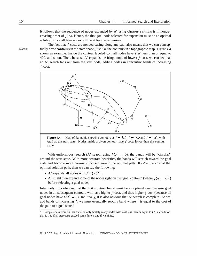
104 Chapter 4. Informed Search and Exploration
It follows that the sequence of nodes expanded by A� using GRAPH-SEARCH is in nonde-creasing order of ����. Hence, the first goal node selected for expansion must be an optimalsolution, since all later nodes will be at least as expensive.
The fact that � -costs are nondecreasing along any path also means that we can concep-tually draw contours in the state space, just like the contours in a topographic map. Figure 4.4CONTOURS
shows an example. Inside the contour labeled ���, all nodes have ���� less than or equal to400, and so on. Then, because A� expands the fringe node of lowest � -cost, we can see thatan A� search fans out from the start node, adding nodes in concentric bands of increasing� -cost.
O
Z
A
T
L
M
DC
R
F
P
G
BU
H
E
V
I
N
380
400
420
S
Figure 4.4 Map of Romania showing contours at � � ���, � � ��� and � � ���, withArad as the start state. Nodes inside a given contour have � -costs lower than the contourvalue.
With uniform-cost search (A� search using ���� � �), the bands will be “circular”around the start state. With more accurate heuristics, the bands will stretch toward the goalstate and become more narrowly focused around the optimal path. If �� is the cost of theoptimal solution path, then we can say the following:
� A� expands all nodes with ���� � ��.
� A� might then expand some of the nodes right on the “goal contour” (where ���� � ��)before selecting a goal node.
Intuitively, it is obvious that the first solution found must be an optimal one, because goalnodes in all subsequent contours will have higher � -cost, and thus higher �-cost (because allgoal nodes have ���� � �). Intuitively, it is also obvious that A� search is complete. As weadd bands of increasing � , we must eventually reach a band where � is equal to the cost ofthe path to a goal state.4
� Completeness requires that there be only finitely many nodes with cost less than or equal to ��, a condition
that is true if all step costs exceed some finite � and if � is finite.
c� 2002 by Russell and Norvig. DRAFT---DO NOT DISTRIBUTE

Section 4.1. Informed (Heuristic) Search Strategies 105
Notice that A� expands no nodes with ���� � ��—for example, Timisoara is not ex-panded in Figure 4.3 even though it is a child of the root. We say that the subtree belowTimisoara is pruned; because ���� is admissible, the algorithm can safely ignore this sub-PRUNING
tree while still guaranteeing optimality. The concept of pruning—eliminating possibilitiesfrom consideration without having to examine them—is important for many areas of AI.
One final observation is that among optimal algorithms of this type—algorithms thatextend search paths from the root—A� is optimally efficient for any given heuristic function.OPTIMALLY
EFFICIENT
That is, no other optimal algorithm is guaranteed to expand fewer nodes than A� (exceptpossibly through tie-breaking among nodes with �������). This is because any algorithmthat does not expand all nodes with ���� � �� runs the risk of missing the optimal solution.
That A� search is complete, optimal, and optimally efficient among all such algorithmsis rather satisfying. Unfortunately, it does not mean that A� is the answer to all our searchingneeds. The catch is that, for most problems, the number of nodes within the goal contoursearch space is still exponential in the length of the solution. Although the proof of the resultis beyond the scope of this book, it has been shown that exponential growth will occur unlessthe error in the heuristic function grows no faster than the logarithm of the actual path cost.In mathematical notation, the condition for subexponential growth is that
������ ������ � �� �������
where ����� is the true cost of getting from � to the goal. For almost all heuristics in practicaluse, the error is at least proportional to the path cost, and the resulting exponential growtheventually overtakes any computer. For this reason, it is often impractical to insist on findingan optimal solution. One can use variants of A� that find suboptimal solutions quickly, or onecan sometimes design heuristics that are more accurate, but not strictly admissible. In anycase, the use of a good heuristic still provides enormous savings compared to the use of anuninformed search. In Section 4.2, we will look at the question of designing good heuristics.
Computation time is not, however, A�’s main drawback. Because it keeps all generatednodes in memory (as do all GRAPH-SEARCH algorithms), A� usually runs out of space longbefore it runs out of time. For this reason, A� is not practical for many large-scale prob-lems. Recently developed algorithms have overcome the space problem without sacrificingoptimality or completeness, at a small cost in execution time. These are discussed next.
Memory-bounded heuristic search
The simplest way to reduce memory requirements for A� is to adapt the idea of iterative deep-ening to the heuristic search context, resulting in the iterative-deepening A� (IDA�) algorithm.The main difference between IDA� and standard iterative deepening is that the cutoff used isthe � -cost (� � �) rather than the depth; at each iteration, the cutoff value is the smallest � -cost of any node that exceeded the cutoff on the previous iteration. IDA� is practical for manyproblems with unit step costs and avoids the substantial overhead associated with keeping asorted queue of nodes. Unfortunately, it suffers from the same difficulties with real-valuedcosts as does the iterative version of uniform-cost search described in Exercise 3.11. Thissection briefly examines two more recent algorithms, called RBFS and MA�.
Recursive best-first search (RBFS) is a simple recursive algorithm that attempts toRECURSIVEBEST-FIRST SEARCH
c� 2002 by Russell and Norvig. DRAFT---DO NOT DISTRIBUTE

106 Chapter 4. Informed Search and Exploration
function RECURSIVE-BEST-FIRST-SEARCH( problem) returns a solution, or failureRBFS( problem, MAKE-NODE(INITIAL-STATE[problem]),�)
function RBFS( problem, node, f-limit) returns a solution, or failure and a new � -cost limitif GOAL-TEST[problem](state) then return nodesuccessors� EXPAND(node, problem)if successors is empty, then return failure,�for each s in successors do � [s]�����s� � ��s�� � node�� endrepeat
best� the lowest � -value node in successorsif � best� � f-limit then return failure, � [best]alternative� the second-lowest � -value among successorsresult,� [best]�RBFS(problem, best,����f-limit� alternative�)if result �� failure then return result
end
Figure 4.5 The algorithm for recursive best-first search.
mimic the operation of standard best-first search, but using only linear space. The algorithm isshown in Figure 4.5. Its structure is similar to that of a recursive depth-first search, but ratherthan continuing indefinitely down the current path, it keeps track of the � -value of the bestalternative path available from any ancestor of the current node. If the current node exceedsthis limit, the recursion unwinds back to the alternative path. As the recursion unwinds, RBFSreplaces the � -value of each node along the path with the best � -value of its children. In thisway, RBFS remembers the � -value of the best leaf in the forgotten subtree and can thereforedecide whether it’s worth reexpanding the subtree at some later time. Figure 4.6 shows howRBFS reaches Bucharest.
RBFS is somewhat more efficient than IDA�, but still suffers from excessive node re-generation. In the example in Figure 4.6, RBFS first follows the path via Rimnicu Vilcea,then “changes its mind” and tries Fagaras, and then changes its mind back again. These mindchanges occur because every time the current best path is extended, there is a good chancethat its � -value will increase—� is usually less optimistic for nodes closer to the goal. Whenthis happens, particularly in large search spaces, the second-best path might become the bestpath, so the search has to backtrack to follow it. Each mind change corresponds to an iterationof IDA�, and could require many reexpansions of forgotten nodes to recreate the best pathand extend it one more node.
Like A�, RBFS is an optimal algorithm if the heuristic function ���� is admissible. Itsspace complexity is ���, but its time complexity is rather difficult to characterize: it de-pends both on the accuracy of the heuristic function and on how often the best path changes asnodes are expanded. Both IDA� and RBFS are subject to the potentially exponential increasein complexity associated with searching on graphs (see Section 3.5), because they cannotcheck for repeated states other than those on the current path.
IDA� and RBFS suffer from using too little memory. Between iterations, IDA� retains
c� 2002 by Russell and Norvig. DRAFT---DO NOT DISTRIBUTE

Section 4.1. Informed (Heuristic) Search Strategies 107
Zerind
Arad
Sibiu
Arad
Timisoara
Fagaras Oradea
Craiova Pitesti Sibiu
Bucharest Craiova Rimnicu Vilcea
Zerind
Arad
Sibiu
Arad
Timisoara
Sibiu Bucharest
Rimnicu VilceaOradea
Zerind
Arad
Sibiu
Arad
Timisoara
Fagaras Oradea Rimnicu Vilcea
Craiova Pitesti Sibiu
646 415 526
526 417 553
646 526
450591
646 526
526 553
418 615 607
447 449
447
447 449
449
366
393
366
393
413
413 417415
366
393
415 450417
417
Rimnicu Vilcea
Fagaras
447
415
447
447
417
(a) After expanding Arad, Sibiu, Rimnicu Vilcea
(c) After switching back to Rimnicu Vilcea and expanding Pitesti
(b) After unwinding back to Sibiu and expanding Fagaras
447
447
Figure 4.6 Stages in an RBFS search for the shortest route to Bucharest. The � -limitvalue for each recursive call is shown on top of each current node. (a) The path via RimnicuVilcea is followed until the current best leaf (Pitesti) has a value that is worse than the bestalternative path (Fagaras). (b) The recursion unwinds and the best leaf value of the forgottensubtree (417) is backed up to Rimnicu Vilcea; then Fagaras is expanded, revealing a bestleaf value of 450. (c) The recursion unwinds and the best leaf value of the forgotten subtree(450) is backed up to Fagaras; then Rimnicu Vilcea is expanded. This time, because the bestalternative path (through Timisoara) costs at least 447, the expansion continues to Bucharest.
only a single number: the current � -cost limit. RBFS retains more information in memory,but it uses only ��� memory: it cannot make use of more memory even if it is available.
It seems sensible, therefore, to use all available memory. Two algorithms that do this areMA� (memory-bounded A�) and SMA� (simplified MA�). We will describe SMA�, whichMA
�
SMA� is—well—simpler. SMA� proceeds just like A�, expanding the best leaf until memory is full.
c� 2002 by Russell and Norvig. DRAFT---DO NOT DISTRIBUTE

108 Chapter 4. Informed Search and Exploration
At this point, it cannot add a new node to the search tree without dropping an old one. SMA�
always drops the worst leaf node—the one with the highest � -value. Like RBFS, SMA�
then backs up the value of the forgotten node to its parent. In this way, the ancestor of aforgotten subtree knows the quality of the best path in that subtree. With this information,SMA� regenerates the subtree only when all other paths have been shown to look worse thanthe path it has forgotten. Another way of saying this is that, if all the descendants of a node �are forgotten, then we will not know which way to go from �, but we will still have an ideaof how worthwhile it is to go anywhere from �.
The complete algorithm is too complicated to reproduce here,5 but there is one subtletyworth mentioning. We said that SMA� expands the best leaf and deletes the worst leaf. Whatif all the leaf nodes have the same � -value? Then the algorithm might select the same nodefor deletion and expansion. SMA� solves this problem by expanding the newest best leaf anddeleting the oldest worst leaf. These can be the same node only if there is only one leaf; in thatcase, the current search tree must be a single path from root to leaf that fills all of memory.If the leaf is not a goal node, then even if it is on an optimal solution path, that solution isnot reachable with the available memory. Therefore, the node can be discarded exactly as ifit had no successors.
SMA� is complete if there is any reachable solution—that is, if �, the depth of theshallowest goal node, is less than the memory size (expressed in nodes). It is optimal if anyoptimal solution is reachable; otherwise it returns the best reachable solution. In practicalterms, SMA� might well be the best general-purpose algorithm for finding optimal solutions,particularly when the state space is a graph, step costs are not uniform, and node generationis expensive compared to the additional overhead of maintaining the open and closed lists.
On very hard problems, however, it will often be the case that SMA� is forced to switchback and forth continually between a set of candidate solution paths, only a small subset ofwhich can fit in memory. (This resembles the problem of thrashing in disk paging systems.)THRASHING
Then the extra time required for repeated regeneration of the same nodes means that problemsthat would be practically solvable by A�, given unlimited memory, become intractable forSMA�. That is to say, memory limitations can make a problem intractable from the point ofview of computation time. Although there is no theory to explain the tradeoff between timeand memory, it seems that this is an inescapable problem. The only way out is to drop theoptimality requirement.
Learning to search better
We have presented several fixed strategies—breadth-first, greedy best-first, and so on—thathave been designed by computer scientists. Could an agent learn how to search better? Theanswer is yes, and the method rests on an important concept called the metalevel state space.METALEVEL STATE
SPACE
Each state in a metalevel state space captures the internal (computational) state of a programthat is searching in an object-level state space such as Romania. For example, the internalOBJECT-LEVEL STATE
SPACE
state of the A� algorithm consists of the current search tree. Each action in the metalevel statespace is a computation step that alters the internal state; for example, each computation step
� A rough sketch appeared in the first edition of this book.
c� 2002 by Russell and Norvig. DRAFT---DO NOT DISTRIBUTE

Section 4.2. Heuristic Functions 109
in A� expands a leaf node and adds its successors to the tree. Thus, Figure 4.3, which showsa sequence of larger and larger search trees, can be seen as depicting a path in the metalevelstate space.
Now, the path in Figure 4.3 has five steps, including one step—the expansion of Fagaras—that is not especially helpful. For harder problems, there will be many such missteps, and ametalevel learning algorithm can learn from these experiences to avoid exploring unpromis-METALEVEL
LEARNING
ing subtrees. The techniques used for this kind of learning are described in Chapter 19; thegoal is to minimize the total cost of problem solving, trading off computational expense andpath cost.
4.2 HEURISTIC FUNCTIONS
In this section, we will look at heuristics for the 8-puzzle, in order to shed light on the natureof heuristics in general.
The 8-puzzle was one of the earliest heuristic search problems. As mentioned in Sec-tion 3.2, the object of the puzzle is to slide the tiles horizontally or vertically into the emptyspace until the configuration matches the goal configuration (Figure 4.7).
2
Start State Goal State
1
3 4
6 7
5
1
2
3
4
6
7
8
5
8
Figure 4.7 A typical instance of the 8-puzzle. The solution is 26 steps long.
The average solution cost for a randomly generated 8-puzzle instance is about 22 steps.The branching factor is about 3. (When the empty tile is in the middle, there are four possiblemoves; when it is in a corner there are two; and when it is along an edge there are three.) Thismeans that an exhaustive search to depth 22 would look at about ��� � � � ���� states. Bykeeping track of repeated states, we could cut this down by a factor of about 170,000, becausethere are only ��� � ���� ��� distinct states that are reachable. (See Exercise 3.4.) This isa manageable number, but the corresponding number for the 15-puzzle is roughly ����, sothe next order of business is to find a good heuristic function. If we want to find the shortestsolutions by using A�, we need a heuristic function that never overestimates the number ofsteps to the goal. Here are two candidates:
� �� � the number of misplaced tiles. For Figure 4.7, all of the eight tiles are out ofposition, so the start state would have �� � �. �� is an admissible heuristic, because itis clear that any tile that is out of place must be moved at least once.
c� 2002 by Russell and Norvig. DRAFT---DO NOT DISTRIBUTE

110 Chapter 4. Informed Search and Exploration
� �� � the sum of the distances of the tiles from their goal positions. Because tilescannot move along diagonals, the distance we will count is the sum of the horizontaland vertical distances. This is sometimes called the city block distance or Manhattandistance. �� is also admissible, because all any move can do is move one tile one stepMANHATTAN
DISTANCE
closer to the goal. Tiles 1 to 8 in the start state give a Manhattan distance of
�� � � � � � � � � � � � � � � � � � ��
As we would hope, neither of these overestimates the true solution cost, which is 26.
The effect of heuristic accuracy on performance
One way to characterize the quality of a heuristic is the effective branching factor �. If theEFFECTIVEBRANCHING FACTOR
total number of nodes generated by A� for a particular problem is � , and the solution depthis �, then � is the branching factor that a uniform tree of depth � would have to have in orderto contain � � � nodes. Thus,
� � � � � � � � ���� � � ����
For example, if A� finds a solution at depth 5 using 52 nodes, then the effective branchingfactor is 1.92. The effective branching factor can vary across problem instances, but usuallyit is fairly constant for sufficiently hard problems. Therefore, experimental measurements of� on a small set of problems can provide a good guide to the heuristic’s overall usefulness.A well-designed heuristic would have a value of � close to 1, allowing fairly large problemsto be solved.
To test the heuristic functions �� and ��, we generated 1200 random problems withsolution lengths from 2 to 24 (100 for each even number) and solved them with iterativedeepening search and with A� tree search using both �� and ��. Figure 4.8 gives the averagenumber of nodes expanded by each strategy and the effective branching factor. The resultssuggest that �� is better than ��, and is far better than using iterative deepening search. On oursolutions with length 14, A� with �� is 30,000 times more efficient than uninformed iterativedeepening search.
One might ask whether �� is always better than ��. The answer is yes. It is easy to seefrom the definitions of the two heuristics that, for any node �, ����� � �����. We thus saythat �� dominates ��. Domination translates directly into efficiency: A� using �� will neverDOMINATION
expand more nodes than A� using �� (except possibly for some nodes with �������). Theargument is simple. Recall the observation on page 104 that every node with ���� � �� willsurely be expanded. This is the same as saying that every node with ���� � �� � ���� willsurely be expanded. But because �� is at least as big as �� for all nodes, every node that issurely expanded by A� search with �� will also surely be expanded with ��, and �� mightalso cause other nodes to be expanded as well. Hence, it is always better to use a heuristicfunction with higher values, provided it does not overestimate and that the computation timefor the heuristic is not too large.
c� 2002 by Russell and Norvig. DRAFT---DO NOT DISTRIBUTE

Section 4.2. Heuristic Functions 111
Search Cost Effective Branching Factor
� IDS A*(��) A*(��) IDS A*(��) A*(��)
2 10 6 6 2.45 1.79 1.794 112 13 12 2.87 1.48 1.456 680 20 18 2.73 1.34 1.308 6384 39 25 2.80 1.33 1.24
10 47127 93 39 2.79 1.38 1.2212 3644035 227 73 2.78 1.42 1.2414 3473941 539 113 2.83 1.44 1.2316 – 1301 211 – 1.45 1.2518 – 3056 363 – 1.46 1.2620 – 7276 676 – 1.47 1.2722 – 18094 1219 – 1.48 1.2824 – 39135 1641 – 1.48 1.26
Figure 4.8 Comparison of the search costs and effective branching factors for theITERATIVE-DEEPENING-SEARCH and A� algorithms with ��, ��. Data are averaged over100 instances of the 8-puzzle, for various solution lengths.
Inventing admissible heuristic functions
We have seen that both �� (misplaced tiles) and �� (Manhattan distance) are fairly goodheuristics for the 8-puzzle and that �� is better. How might one have come up with ��? Is itpossible for a computer to invent such a heuristic mechanically?
�� and �� are estimates of the remaining path length for the 8-puzzle, but they arealso perfectly accurate path lengths for simplified versions of the puzzle. If the rules of thepuzzle were changed so that a tile could move anywhere, instead of just to the adjacent emptysquare, then �� would give the exact number of steps in the shortest solution. Similarly, ifa tile could move one square in any direction, even onto an occupied square, then �� wouldgive the exact number of steps in the shortest solution. A problem with fewer restrictions onthe actions is called a relaxed problem. The cost of an optimal solution to a relaxed problemRELAXED PROBLEM
is an admissible heuristic for the original problem. The heuristic is admissible becausethe optimal solution in the original problem is, by definition, also a solution in the relaxedproblem and therefore must be at least as expensive as the optimal solution in the relaxedproblem. Because the derived heuristic is an exact cost for the relaxed problem, it must obeythe triangle inequality and is therefore consistent (see page 103).
If a problem definition is written down in a formal language, it is possible to constructrelaxed problems automatically.6 For example, if the 8-puzzle actions are described as
A tile can move from square A to square B ifA is horizontally or vertically adjacent to B and B is blank,
� In Chapters 8 and 11, we will describe formal languages suitable for this task. For now, we will use English.
c� 2002 by Russell and Norvig. DRAFT---DO NOT DISTRIBUTE
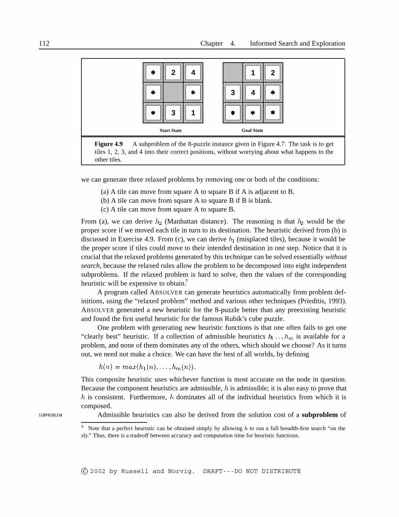
112 Chapter 4. Informed Search and Exploration
2
Start State Goal State
1
3 6
7 8
5
1
2
3
4
6
8
5 4
Figure 4.9 A subproblem of the 8-puzzle instance given in Figure 4.7. The task is to gettiles 1, 2, 3, and 4 into their correct positions, without worrying about what happens to theother tiles.
we can generate three relaxed problems by removing one or both of the conditions:
(a) A tile can move from square A to square B if A is adjacent to B.(b) A tile can move from square A to square B if B is blank.(c) A tile can move from square A to square B.
From (a), we can derive �� (Manhattan distance). The reasoning is that �� would be theproper score if we moved each tile in turn to its destination. The heuristic derived from (b) isdiscussed in Exercise 4.9. From (c), we can derive �� (misplaced tiles), because it would bethe proper score if tiles could move to their intended destination in one step. Notice that it iscrucial that the relaxed problems generated by this technique can be solved essentially withoutsearch, because the relaxed rules allow the problem to be decomposed into eight independentsubproblems. If the relaxed problem is hard to solve, then the values of the correspondingheuristic will be expensive to obtain.7
A program called ABSOLVER can generate heuristics automatically from problem def-initions, using the “relaxed problem” method and various other techniques (Prieditis, 1993).ABSOLVER generated a new heuristic for the 8-puzzle better than any preexisting heuristicand found the first useful heuristic for the famous Rubik’s cube puzzle.
One problem with generating new heuristic functions is that one often fails to get one“clearly best” heuristic. If a collection of admissible heuristics �� �� is available for aproblem, and none of them dominates any of the others, which should we choose? As it turnsout, we need not make a choice. We can have the best of all worlds, by defining
���� � ���������� � ������
This composite heuristic uses whichever function is most accurate on the node in question.Because the component heuristics are admissible, � is admissible; it is also easy to prove that� is consistent. Furthermore, � dominates all of the individual heuristics from which it iscomposed.
Admissible heuristics can also be derived from the solution cost of a subproblem ofSUBPROBLEM
� Note that a perfect heuristic can be obtained simply by allowing � to run a full breadth-first search “on thesly.” Thus, there is a tradeoff between accuracy and computation time for heuristic functions.
c� 2002 by Russell and Norvig. DRAFT---DO NOT DISTRIBUTE

Section 4.2. Heuristic Functions 113
a given problem. For example, Figure 4.9 shows a subproblem of the 8-puzzle instancein Figure 4.7. The subproblem involves getting tiles 1, 2, 3, 4 into their correct positions.Clearly, the cost of the optimal solution of this subproblem is a lower bound on the cost ofthe complete problem. It turns out to be substantially more accurate than Manhattan distancein some cases.
The idea behind pattern databases is to store these exact solution costs for every pos-PATTERN DATABASES
sible subproblem instance—in our example, every possible configuration of the four tiles andthe blank. (Notice that the locations of the other four tiles are irrelevant for the purposes ofsolving the subproblem, but moves of those tiles do count towards the cost.) Then, we com-pute an admissible heuristic ��� for each complete state encountered during a search simplyby looking up the corresponding subproblem configuration in the database. The databaseitself is constructed by searching backwards from the goal state and recording the cost ofeach new pattern encountered; the expense of this search is amortized over many subsequentproblem instances.
The choice of 1-2-3-4 is fairly arbitrary; we could also construct databases for 5-6-7-8,and for 2-4-6-8, and so on. Each database yields an admissible heuristic, and these heuristicscan be combined, as explained earlier, by taking the maximum value. A combined heuristic ofthis kind is much more accurate than the Manhattan distance; the number of nodes generatedwhen solving random 15-puzzles can be reduced by a factor of 1000.
One might wonder whether the heuristics obtained from the 1-2-3-4 database and the5-6-7-8 could be added, since the two subproblems seem not to overlap. Would this still givean admissible heuristic? The answer is no, because the solutions of the 1-2-3-4 subproblemand the 5-6-7-8 subproblem for a given state will almost certainly share some moves—it isunlikely that 1-2-3-4 can be moved into place without touching 5-6-7-8, and vice versa. Butwhat if we don’t count those moves? That is, we record not the total cost of solving the1-2-3-4 subproblem, but just the number of moves involving 1-2-3-4. Then it is easy to seethat the sum of the two costs is still a lower bound on the cost of solving the entire problem.This is the idea behind disjoint pattern databases. Using such databases, it is possible toDISJOINT PATTERN
DATABASES
solve random 15-puzzles in a few milliseconds—the number of nodes generated is reducedby a factor of 10,000 compared with using Manhattan distance. For 24-puzzles, a speedup ofroughly a million can be obtained.
Disjoint pattern databases work for sliding-tile puzzles because the problem can bedivided up in such a way that each move affects only one subproblem—because only one tileis moved at a time. For a problem such as Rubik’s cube, this kind of subdivision cannot bedone because each move affects 8 or 9 of the 26 cubies. Currently, it is not clear how to definedisjoint databases for such problems.
Learning heuristics from experience
A heuristic function ���� is supposed to estimate the cost of a solution beginning from thestate at node �. How could an agent construct such a function? One solution was given in thepreceding section—namely, to devise relaxed problems for which an optimal solution can befound easily. Another solution is to learn from experience. “Experience” here means solving
c� 2002 by Russell and Norvig. DRAFT---DO NOT DISTRIBUTE

114 Chapter 4. Informed Search and Exploration
lots of 8-puzzles, for instance. Each optimal solution to an 8-puzzle problem provides ex-amples from which ���� can be learned. Each example consists of a state from the solutionEXAMPLES
path and the actual cost of the solution from that point. From these examples, an inductivelearning algorithm can be used to construct a function ���� that can (with luck) predict solu-tion costs for other states that arise during search. Techniques for doing just this using neuralnets, decision trees, and other methods are demonstrated in Chapter 18. (The reinforcementlearning methods described in Chapter 19 are also applicable.)
Inductive learning methods work best when supplied with features of a state that areFEATURES
relevant to its evaluation, rather than with just the raw state description. For example, thefeature “number of misplaced tiles” might be helpful in predicting the actual distance of astate from the goal. Let’s call this feature �����. We could take 100 randomly generated8-puzzle configurations and gather statistics on their actual solution costs. We might find thatwhen ����� is 5, the average solution cost is around 14, and so on. Given these data, thevalue of �� can be used to predict ����. Of course, we can use several features. A secondfeature ����� might be “number of pairs of adjacent tiles that are also adjacent in the goalstate.” How should ����� and ����� be combined to predict ����? A common approach isto use a linear combination:
���� � ������� � �������
The constants �� and �� are adjusted to give the best fit to the actual data on solution costs.Presumably, �� should be positive and �� should be negative.
4.3 LOCAL SEARCH ALGORITHMS AND OPTIMIZATION PROBLEMS
The search algorithms that we have seen so far are designed to explore search spaces sys-tematically. This systematicity is achieved by keeping one or more paths in memory and byrecording which alternatives have been explored at each point along the path and which havenot. When a goal is found, the path to that goal also constitutes a solution to the problem.
In many problems, however, the path to the goal is irrelevant. For example, in the 8-queens problem (see page 69), what matters is the final configuration of queens, not the orderin which they are added. This class of problems includes many important applications such asintegrated-circuit design, factory-floor layout, job-shop scheduling, automatic programming,telecommunications network optimization, vehicle routing, and portfolio management.
If the path to the goal does not matter, we might consider a different class of algo-rithms, ones that do not worry about paths at all. Local search algorithms operate usingLOCAL SEARCH
a single current state (rather than multiple paths) and generally move only to neighborsCURRENT STATE
of that state. Typically, the paths followed by the search are not retained. Although localsearch algorithms are not systematic, they have two key advantages: (1) they use very littlememory—usually a constant amount; and (2) they can often find reasonable solutions in largeor infinite (continuous) state spaces for which systematic algorithms are unsuitable.
In addition to finding goals, local search algorithms are useful for solving pure op-timization problems, in which the aim is to find the best state according to an objectiveOPTIMIZATION
PROBLEMS
c� 2002 by Russell and Norvig. DRAFT---DO NOT DISTRIBUTE

Section 4.3. Local Search Algorithms and Optimization Problems 115
function. Many optimization problems do not fit the “standard” search model introduced inOBJECTIVEFUNCTION
Chapter 3. For example, nature provides an objective function—reproductive fitness—thatDarwinian evolution could be seen as attempting to optimize, but there is no “goal test” andno “path cost” for this problem.
To understand local search, we will find it very useful to consider the state space land-scape (as in Figure 4.10). A landscape has both “location” (defined by the state) and “eleva-STATE SPACE
LANDSCAPE
tion” (defined by the value of the heuristic cost function or objective function). If elevationcorresponds to cost, then the aim is to find the lowest valley—a global minimum; if eleva-GLOBAL MINIMUM
tion corresponds to an objective function, then the aim is to find the highest peak—a globalmaximum. (You can convert from one to the other just by inserting a minus sign.) LocalGLOBAL MAXIMUM
search algorithms explore this landscape. A complete local search algorithm always finds agoal if one exists; an optimal algorithm always finds a global minimum/maximum.
currentstate
objective function
state space
global maximum
local maximum
"flat" local maximum
shoulder
Figure 4.10 A one-dimensional state space landscape in which elevation corresponds tothe objective function. The aim is to find the global maximum. Hill-climbing search modifiesthe current state to try to improve it, as shown by the arrow. The various topographic featuresare defined in the text.
Hill-Climbing Search
The hill-climbing search algorithm is shown in Figure 4.11. It is simply a loop that continu-HILL-CLIMBING
ally moves in the direction of increasing value—that is, uphill. It terminates when it reaches a“peak” where no neighbor has a higher value. The algorithm does not maintain a search tree,so the current node data structure need only record the state and its objective function value.Hill-climbing does not look ahead beyond the immediate neighbors of the current state. Thisresembles trying to find the top of Mount Everest in a thick fog while suffering from amnesia.
To illustrate hill-climbing, we will use the 8-queens problem introduced on page 69.Local-search algorithms typically use a complete-state formulation, where each state has8 queens on the board, one per column. The successor function returns all possible statesgenerated by moving a single queen to another square in the same column (so each state has
c� 2002 by Russell and Norvig. DRAFT---DO NOT DISTRIBUTE

116 Chapter 4. Informed Search and Exploration
function HILL-CLIMBING( problem) returns a state that is a local maximuminputs: problem, a problemlocal variables: current, a node
neighbor, a node
current�MAKE-NODE(INITIAL-STATE[problem])loop do
neighbor� a highest-valued successor of currentif VALUE[neighbor]� VALUE[current] then return STATE[current]current� neighbor
end
Figure 4.11 The hill-climbing search algorithm (steepest ascent version), which is themost basic local search technique. At each step the current node is replaced by the bestneighbor; in this version, that means the neighbor with the highest VALUE, but if a heuristiccost estimate � is used, we would find the neighbor with the lowest �.
� �� �� successors). The heuristic cost function � is the number of pairs of queens thatare attacking each other, either directly or indirectly. The global minimum of this functionis zero, which occurs only at perfect solutions. Figure 4.12(a) shows a state with ����.The figure also shows the values of all its successors, with the best successors having ����.Hill-climbing algorithms typically choose randomly among the set of best successors, if thereis more than one.
Hill climbing is sometimes called greedy local search because it grabs a good neighborGREEDY LOCALSEARCH
state without thinking ahead about where to go next. Although greed is considered one of theseven deadly sins, it turns out that greedy algorithms often perform quite well. Hill climbingoften makes very rapid progress towards a solution, because it is usually quite easy to improvea bad state. For example, from the state in Figure 4.12(a), it takes just five steps to reach thestate in Figure 4.12(b), which has ��� and is very nearly a solution. Unfortunately, hillclimbing often gets stuck for the following reasons:
� Local maxima: a local maximum is a peak that is higher than each of its neighboringstates, but lower than the global maximum. Hill-climbing algorithms that reach thevicinity of a local maximum will be drawn upwards towards the peak, but will then bestuck with nowhere else to go. Figure 4.10 illustrates the problem schematically. Moreconcretely, the state in Figure 4.12(b) is in fact a local maximum (i.e., a local minimumfor the cost �); every move of a single queen makes the situation worse.
� Ridges: a ridge is shown in Figure 4.13. Ridges result in a sequence of local maximathat is very difficult for greedy algorithms to navigate.
� Plateaux: a plateau is an area of the state space landscape where the evaluation functionis flat. It can be a flat local maximum, from which no uphill exit exists, or a shoulder,SHOULDER
from which it is possible to make progress. (See Figure 4.10.) A hill-climbing searchmight be unable to find its way off the plateau.
c� 2002 by Russell and Norvig. DRAFT---DO NOT DISTRIBUTE

Section 4.3. Local Search Algorithms and Optimization Problems 117
14
18
17
15
14
18
14
14
14
14
14
12
16
12
13
16
17
14
18
13
14
17
15
18
15
13
15
13
12
15
15
13
15
12
13
14
14
14
16
12
14
12
12
15
16
13
14
12
14
18
16
16
16
14
16
14
(a) (b)
Figure 4.12 (a) An 8-queens state with heuristic cost estimate ����, showing the valueof � for each possible successor obtained by moving a queen within its column. The bestmoves are marked. (b) A local minimum in the 8-queens state space; the state has ��� butevery successor has a higher cost.
In each case, the algorithm reaches a point at which no progress is being made. Startingfrom a randomly generated 8-queens state, steepest-ascent hill climbing gets stuck 86% ofthe time, solving only 14% of problem instances. Still, it works quickly, taking just 4 stepson average when it succeeds and 3 when it gets stuck—not bad for a state space with �� � ��million states.
The algorithm in Figure 4.11 halts if it reaches a plateau where the best successor hasthe same value as the current state. Might it not be a good idea to keep going—to allow asideways move in the hope that the plateau is really a shoulder, as shown in Figure 4.10? TheSIDEWAYS MOVE
answer is usually yes, but we must take care. If we always allow sideways moves when thereare no uphill moves, an infinite loop will occur whenever the algorithm reaches a flat localmaximum that is not a shoulder. One common solution is to put a limit on the number of con-secutive sideways moves allowed. For example, we could allow up to, say, 100 consecutivesideways moves in the 8-queens problem. This raises the percentage of problem instancessolved by hill-climbing from 14% to 94%. Success comes at a cost: the algorithm averagesroughly 21 steps for each successful instance and 64 for each failure.
Variants of the basic hill-climbing method can be defined by changing the way in whichmoves are chosen. For example, stochastic hill climbing chooses at random from amongSTOCHASTIC HILL
CLIMBING
the uphill moves; the probability of selection can vary with the steepness of the uphill move.This usually converges more slowly than steepest ascent, but in some state landscapes itfinds better solutions. First-choice hill climbing implements stochastic hill climbing byFIRST-CHOICE HILL
CLIMBING
generating successors randomly until one is generated that is better than the current state.
c� 2002 by Russell and Norvig. DRAFT---DO NOT DISTRIBUTE

118 Chapter 4. Informed Search and Exploration
Figure 4.13 Illustration of why ridges cause difficulties for hill-climbing. The grid ofstates (dark circles) is superimposed on a ridge rising from left to right, creating a sequenceof local maxima that are not directly connected to each other. From each local maximum, allthe available actions point downhill.
This is a good strategy when a state has many (e.g., thousands) of successors. Exercise 4.16asks you to investigate.
The hill-climbing algorithms described so far are incomplete—they often fail to finda goal when one exists because they can get stuck on local maxima. Random-restart hillclimbing adopts the well known adage, “If at first you don’t succeed, try, try again.” ItRANDOM-RESTART
HILL CLIMBING
conducts a series of hill-climbing searches from randomly generated initial states,8 stoppingwhen a goal is found. It is complete (if we do not limit the number of restarts) with probabilityapproaching 1, for the trivial reason that it will eventually generate a goal state as the initialstate. (It is also optimal for optimization problems, for the same reason, but it has no way torecognize an optimal solution.) If each hill-climbing search has a probability � of success,then the expected number of restarts required is ���. For 8-queens instances with no sidewaysmoves allowed, � � � ��, so we need roughly 7 iterations to find a goal (6 failures and 1success). The expected number of steps is the cost of one successful iteration plus ��� ����times the cost of failure, or roughly 22 steps. When we allow sideways moves, ��� � � � ��iterations are needed on average and �� ��� � �� ���� �� �� � �� steps. For 8-queens,then, random-restart hill climbing is very effective indeed. Even for three million queens, theapproach can find solutions in under a minute.9
The success of hill climbing depends very much on the shape of the state-space land-
� Generating a random state from an implicitly specified state space can be a hard problem in itself. Luby et al. (1993) prove that it is best, in some cases, to restart a randomized search algorithm after a particular,fixed amount of time and that this can be much more efficient than letting each search continue indefinitely.Disallowing or limiting the number of sideways moves is an example of this.
c� 2002 by Russell and Norvig. DRAFT---DO NOT DISTRIBUTE

Section 4.3. Local Search Algorithms and Optimization Problems 119
scape: if there are few local maxima and plateaux, random-restart hill climbing will find agood solution very quickly. On the other hand, many real problems have a landscape thatlooks more like a family of porcupines on a flat floor, with miniature porcupines living on thetip of each porcupine needle, ad infinitum. NP-hard problems typically have an exponentialnumber of local maxima to get stuck on. Despite this, a reasonably good local maximum canoften be found after a small number of restarts.
Simulated annealing search
A hill-climbing algorithm that never makes “downhill” moves towards states with lower value(or higher cost) is guaranteed to be incomplete, because it can get stuck on a local maximum.In contrast, a purely random walk—that is, moving to a successor chosen uniformly at ran-dom from the set of successors—is complete, but extremely inefficient. Therefore, it seemsreasonable to try to combine hill climbing with a random walk in some way that yields bothefficiency and completeness. Simulated annealing is such an algorithm. In metallurgy, an-SIMULATED
ANNEALING
nealing is the process used to temper or harden metals and glass by heating them to a hightemperature and then gradually cooling them, thus allowing the material to coalesce into alow-energy crystalline state. To understand simulated annealing, let’s switch our point ofview from hill climbing to gradient descent (i.e., minimizing cost) and imagine the task ofGRADIENT DESCENT
getting a Ping-Pong ball into the deepest crevice in a bumpy surface. If we just let the ballroll, it will come to rest at a local minimum. If we shake the surface, we can bounce the ballout of the local minimum. The trick is to shake just hard enough to bounce the ball out oflocal minima, but not hard enough to dislodge it from the global minimum. The simulated-annealing solution is to start by shaking hard (i.e., at a high temperature) and then graduallyreduce the intensity of the shaking (i.e., lower the temperature).
The innermost loop of the simulated-annealing algorithm (Figure 4.14) is quite similarto hill climbing. Instead of picking the best move, however, it picks a random move. If themove improves the situation, it is always accepted. Otherwise, the algorithm accepts the movewith some probability less than 1. The probability decreases exponentially with the “badness”of the move—the amount �E by which the evaluation is worsened. The probability alsodecreases as the “temperature” T goes down: “bad” moves are more likely to be allowed atthe start when temperature is high, and they become more and more unlikely as T decreases.The schedule input determines the value of T as a function of time. One can prove that if theschedule lowers T slowly enough, the algorithm will find a global optimum with probabilityapproaching 1.
Simulated annealing was first used extensively to solve VLSI layout problems in theearly 1980s. It has been applied widely to factory scheduling and other large-scale optimiza-tion tasks. In Exercise 4.16, you are asked to compare its performance to that of random-restart hill climbing on the �-queens puzzle.
Local beam search
Keeping just one node in memory might seem to be an extreme reaction to the problem ofmemory limitations. The local beam search algorithm10 keeps track of � states rather thanLOCAL BEAM
SEARCH
c� 2002 by Russell and Norvig. DRAFT---DO NOT DISTRIBUTE

120 Chapter 4. Informed Search and Exploration
function SIMULATED-ANNEALING( problem, schedule) returns a solution stateinputs: problem, a problem
schedule, a mapping from time to “temperature”local variables: current, a node
next, a nodeT, a “temperature” controlling the probability of downward steps
current�MAKE-NODE(INITIAL-STATE[problem])for t� 1 to� do
T� schedule[t]if T = 0 then return currentnext� a randomly selected successor of current�E�VALUE[next] – VALUE[current]if �E � 0 then current� nextelse current� next only with probability �����
Figure 4.14 The simulated annealing search algorithm, a version of stochastic hill climb-ing where some downhill moves are allowed. Downhill moves are accepted readily early inthe annealing schedule and then less often as time goes on.
just one. It begins with � randomly generated states. At each step, all the successors of all �states are generated. If any one is a goal, the algorithm halts. Otherwise, it selects the � bestsuccessors from the complete list and repeats.
At first sight, a local beam search with � states might seem to be nothing more thanrunning � random restarts in parallel instead of in sequence. In fact, the two algorithmsare quite different. In a random-restart search, each search process runs independently ofthe others. In a local beam search, useful information is passed among the � parallel searchthreads. For example, if one state generates several good successors and the other ��� statesall generate bad successors, then the effect is that the first state says to the others, “Come overhere, the grass is greener!” The algorithm quickly abandons unfruitful searches and movesits resources to where the most progress is being made.
In its simplest form, local beam search can suffer from a lack of diversity among the� states—they can quickly become concentrated in a small region of the state space, makingthe search little more than an expensive version of hill climbing. A variant called stochasticbeam search, analogous to stochastic hill climbing, helps to alleviate this problem. InsteadSTOCHASTIC BEAM
SEARCH
of choosing the best � from the the pool of candidate successors, stochastic beam searchchooses � successors at random, with the probability of choosing a given successor beingan increasing function of its value. Stochastic beam search bears some resemblance to theprocess of natural selection, whereby the “successors” (offspring) of a “state” (organism)populate the next generation according to its “value” (fitness).
� Local beam search is an adaptation of beam search, which is a path-based algorithm.
c� 2002 by Russell and Norvig. DRAFT---DO NOT DISTRIBUTE

Section 4.3. Local Search Algorithms and Optimization Problems 121
32252124
(a)Initial Population
(b)Fitness Function
(c)Selection
(d)Cross−Over
(e)Mutation
24748552
32752411
24415124
24
23
20
32543213 11
29%
31%
26%
14%
32752411
24748552
32752411
24415124
32748552
24752411
32752124
24415411
24752411
32748152
24415417
Figure 4.15 The genetic algorithm. The initial population in (a) is ranked by the fitnessfunction in (b), resulting in pairs for mating in (c). They produce offspring in (d), which aresubject to mutation in (e).
Genetic Algorithms
A genetic algorithm (or GA) is a variant of stochastic beam search in which successor statesGENETICALGORITHM
are generated by combining two parent states, rather than by modifying a single state. Theanalogy to natural selection is the same as in stochastic beam search, except now we aredealing with sexual rather than asexual reproduction.
Like beam search, GAs begin with a set of � randomly generated states, called thepopulation. Each state, or individual, is represented as a string over a finite alphabet—mostPOPULATION
INDIVIDUAL commonly, a string of 0s and 1s. For example, an 8-queens state must specify the positions of8 queens, each in a column of 8 squares, and so requires � �� ���� bits. Alternatively,the state could be represented as 8 digits, each in the range from 1 to 8. (We will see laterthat the two encodings behave differently.) Figure 4.15(a) shows a population of four 8-digitstrings representing 8-queens states.
The production of the next generation of states is shown in Figure 4.15(b)–(e). In (b),each state is rated by the evaluation function or (in GA terminology) the fitness function.FITNESS FUNCTION
A fitness function should return higher values for better states, so, for the 8-queens problemwe use the number of nonattacking pairs of queens, which has a value of 28 for a solution.The values of the four states are 24, 23, 20, and 11. In this particular variant of the geneticalgorithm, the probability of being chosen for reproducing is directly proportional to thefitness score, and the percentages are shown next to the raw scores.
In (c), a random choice of two pairs is selected for reproduction, in accordance with theprobabilities in (b). Notice that one individual is selected twice and one not at all.11 For eachpair to be mated, a crossover point is randomly chosen from the positions in the string. InCROSSOVER
Figure 4.15 the crossover points are after the third digit in the first pair and after the fifth digitin the second pair.12
�� There are many variants of this selection rule. The method of culling, in which all individuals below a giventhreshold are discarded, can be shown to converge faster than the random version (Baum et al., 1995).�� It is here that the encoding matters. If a 24-bit encoding is used instead of 8 digits, then the crossover pointhas a 2/3 chance of being in the middle of a digit, which results in an essentially arbitrary mutation of that digit.
c� 2002 by Russell and Norvig. DRAFT---DO NOT DISTRIBUTE

122 Chapter 4. Informed Search and Exploration
+ =
Figure 4.16 The 8-queens states corresponding to the first two parents in Figure 4.15(c)and the first offspring in Figure 4.15(d).
In (d), the offspring themselves are created by crossing over the parent strings at thecrossover point. For example, the first child of the first pair gets the first three digits from thefirst parent and the remaining digits from the second parent, whereas the second child getsthe first three digits from the second parent and the rest from the first parent. The 8-queensstates involved in this reproduction step are shown in Figure 4.16. The example illustratesthe fact that, when two parent states are quite different, the crossover operation can producea state that is a long way from either parent state. It is often the case that the population isquite diverse early on in the process, so crossover (like simulated annealing) frequently takeslarge steps in the state space early in the search process and smaller steps later on when mostindividuals are quite similar.
Finally, in (e), each location is subject to random mutation with a small independentMUTATION
probability. One digit was mutated in the first, third, and fourth offspring. In the 8-queensproblem, this corresponds to choosing a queen at random and moving it to a random squarein its column. Figure 4.17 describes an algorithm that implements all these steps.
Like stochastic beam search, genetic algorithms combine an uphill tendency with ran-dom exploration and exchange of information among parallel search threads. The primaryadvantage, if any, of genetic algorithms comes from the crossover operation. Yet it can beshown mathematically that, if the positions of the genetic code is permuted initially in a ran-dom order, crossover conveys no advantage. Intuitively, the advantage comes from the abilityof crossover to combine large blocks of letters that have evolved independently to performuseful functions, thus raising the level of granularity at which the search operates. For ex-ample, it could be that putting the first three queens in positions 2, 4, and 6 (which results inno attacks) constitutes a useful block that can be combined with other blocks to construct asolution.
The theory of genetic algorithms explains how this works using the idea of a schema,SCHEMA
which is a substring in which some of the positions can be left unspecified. For example,the schema 246***** describes all 8-queens states in which the first three queens are inpositions 2, 4, and 6 respectively. Strings that match the schema (such as 24613578) arecalled instances of the schema. It can be shown that, if the average fitness of the instances ofa schema is above the mean, then the number of instances of the schema within the populationwill grow over time. Clearly, this effect is unlikely to be significant if adjacent bits are totally
c� 2002 by Russell and Norvig. DRAFT---DO NOT DISTRIBUTE

Section 4.3. Local Search Algorithms and Optimization Problems 123
function GENETIC-ALGORITHM( population, FITNESS-FN) returns an individualinputs: population, a set of individuals
FITNESS-FN, a function that measures the fitness of an individual
repeatnew-population� empty setloop for i from 1 to SIZE(population) do���RANDOM-SELECTION( population, FITNESS-FN)���RANDOM-SELECTION( population, FITNESS-FN)child�REPRODUCE( ��� ��)if (small random probability) then child�MUTATE(child)add child to new-population
endpopulation� new-population
until some individual is fit enough, or enough time has elapsedreturn the best individual in population, according to FITNESS-FN
function REPRODUCE( ��� ��) returns an individualinputs: ��� ��, parent individuals
n� LENGTH(��)c� random number from 1 to nreturn APPEND(SUBSTRING(��� �� �), SUBSTRING(��� �� �� ))
Figure 4.17 A genetic algorithm. The algorithm is the same as the one diagrammed inFigure 4.15, with one variation: in this more popular version, each mating of two parentsproduces only one offspring, not two.
unrelated to each other, because then there will be few contiguous blocks that provide aconsistent benefit. Genetic algorithms work best when schemas correspond to meaningfulcomponents of a solution. For example, if the string is a representation of an antenna, thenthe schemas may represent components of the antenna, such as reflectors and deflectors. Agood component is likely to be good in a variety of different designs. This suggests thatthe successful application of genetic algorithms requires careful engineering of the stringrepresentation.
In practice, genetic algorithms have had a widespread impact on optimization problems,such as circuit layout and job-shop scheduling. At present, it is not clear whether the appealof genetic algorithms arises from their performance or from their æsthetically pleasing originsin the theory of evolution. Much work remains to be done to identify the conditions underwhich genetic algorithms perform well.
c� 2002 by Russell and Norvig. DRAFT---DO NOT DISTRIBUTE

124 Chapter 4. Informed Search and Exploration
EVOLUTION AND SEARCH
The basic theory of evolution was developed in Charles Darwin’s On the Ori-gin of Species by Means of Natural Selection (1859). The central idea is simple:variations (known as mutations) occur in reproduction and will be preserved insuccessive generations approxiamtely in proportion to their effect on reproductivefitness.
Darwin’s theory was developed with no knowledge of how the traits of organ-isms can be inherited and modified. The probabilistic laws governing these pro-cesses were first identified by Gregor Mendel (1866), a monk who experimentedwith sweet peas using what he called artificial fertilization. Much later, Watson andCrick (1953) identified the structure of the DNA molecule and its alphabet, AGTC(adenine, guanine, thymine, cytosine). In the standard model, variation occurs bothby point mutations in the letter sequence and by “crossover” (in which the DNA ofan offspring is generated by combining long sections of DNA from each parent).
The analogy to local search algorithms has already been described; the princi-pal difference between stochastic beam search and evolution is the use of sexual re-production, wherein successors are generated from multiple organisms rather thanjust one. The actual mechanisms of evolution are, however, far richer than mostgenetic algorithms allow. For example, mutations can involve reversals, duplica-tions, and movement of large chunks of DNA; some viruses borrow DNA from oneorganism and insert it in another; and there are transposable genes that do nothingbut copy themselves many thousands of times within the genome. There are evengenes that poison cells from potential mates that do not carry the gene, therebyincreasing their chances of replication. Most important is the fact that the genesthemselves encode the mechanisms whereby the genome is reproduced and trans-lated into an organism. In genetic algorithms, those mechanisms are a separateprogram that is not represented within the strings being manipulated.
Darwinian evolution might well seem to be an inefficient mechanism, havinggenerated blindly some ���� or so organisms without improving its search heuris-tics one iota. Fifty years before Darwin, however, the otherwise great French natu-ralist Jean Lamarck (1809) proposed a theory of evolution whereby traits acquiredby adaptation during an organism’s lifetime would be passed on to its offspring.Such a process would be effective, but does not seem to occur in nature. Muchlater, James Baldwin (1896) proposed a superficially similar theory: that behaviorlearned during an organism’s lifetime could accelerate the rate of evolution. UnlikeLamarck’s, Baldwin’s theory is entirely consistent with Darwinian evolution, be-cause it relies on selection pressures operating on individuals that have found localoptima among the set of possible behaviors allowed by their genetic makeup. Mod-ern computer simulations confirm that the “Baldwin effect” is real, provided that“ordinary” evolution can create organisms whose internal performance measure issomehow correlated with actual fitness.
c� 2002 by Russell and Norvig. DRAFT---DO NOT DISTRIBUTE

Section 4.4. Local Search in Continuous Spaces 125
4.4 LOCAL SEARCH IN CONTINUOUS SPACES
In Chapter 2, we explained the distinction between discrete and continuous environments,pointing out that most real-world environments are continuous. Yet none of the algorithmswe have described can handle continuous state spaces—the successor function would in mostcases return infinitely many states! This section provides a very brief introduction to somelocal search techniques for finding optimal solutions in continuous spaces. The literatureon this topic is vast; many of the basic techniques originated in the 17th century, after thedevelopment of calculus by Newton and Leibniz.13 We will find uses for these techniques atseveral places in the book, including the chapters on learning, vision, and robotics.
Let us begin with an example. Suppose we want to place three new airports anywherein Romania, such that the sum of squared distances from each city on the map (Figure 3.2)to its nearest airport is minimized. Then the state space is defined by the coordinates ofthe airports: ���� ���, ���� ���, and ���� ���. This is a six-dimensional space; we also saythat states are defined by six variables. (In general, states are defined by an �-dimensionalvector of variables, x.) Moving around in this space corresponds to moving one or more ofthe airports on the map. The objective function ����� ��� ��� ��� ��� ��� is relatively easy tocompute for any particular state once we compute the closest cities, but rather tricky to writedown in general.
One way to avoid continuous problems is simply to discretize the neighborhood of eachDISCRETIZATION
state. For example, we can move only one airport at a time in either the � or � direction by afixed amount �Æ. With 6 variables, this gives 12 successors for each state. We can then applyany of the local search algorithms described previously. One can also apply stochastic hillclimbing and simulated annealing directly, without discretizing the space. These algorithmschoose successors randomly, which can be done by generating random vectors of length Æ.
There are many methods that attempt to use the gradient of the landscape to find aGRADIENT
maximum. The gradient of the objective function is a vector � that gives the magnitude anddirection of the steepest slope. For our problem, we have
� �
���
������
������
������
������
������
���
�
In some cases, we can find a maximum by solving the equation � ��. (This could be done,for example, if we were placing just one airport; the solution is the arithmetic mean of all thecities’ coordinates.) In many cases, however, this equation cannot be solved in closed form.For example, with three airports, the expression for the gradient depends on what cities areclosest to each airport in the current state. This means we can compute the gradient locallybut not globally. Even so, we can still perform steepest-ascent hill climbing by updating thecurrent state via the formula
x � x � � ��x� �
where � is a small constant. In other cases, the objective function might not be availablein a differentiable form at all—for example, the value of a particular set of airport locations
�� A basic knowledge of multivariate calculus and vector arithmetic is useful when one is reading this section.
c� 2002 by Russell and Norvig. DRAFT---DO NOT DISTRIBUTE

126 Chapter 4. Informed Search and Exploration
may be determined by running some large-scale economic simulation package. In thosecases, a so-called empirical gradient can be determined by evaluating the response to smallEMPIRICAL
GRADIENT
increments and decrements in each coordinate. Empirical gradient search is the same assteepest-ascent hill climbing in a discretized version of the state space.
Hidden beneath the phrase “� is a small constant” lies a huge variety of methods foradjusting �. The basic problem is that, if � is too small, too many steps are needed; if �is too large, the search could overshoot the maximum. The technique of line search tries toLINE SEARCH
overcome this dilemma by extending the current gradient direction—usually by repeatedlydoubling �—until � starts to decrease again. The point at which this occurs becomes the newcurrent state. There are several schools of thought about how the new direction should bechosen at this point.
For many problems, the most effective algorithm is the venerable Newton–RaphsonNEWTON–RAPHSON
method (Newton, 1671; Raphson, 1690). This is a general technique for finding roots offunctions—that is, solving equations of the form ����� �. It works by computing a newestimate for the root � according to Newton’s formula
�� �� ����������
To find a maximum or minimum of � , we need to find x such that the gradient is zero (i.e., ��x�� 0). Thus ���� in Newton’s formula becomes ��x�, and the update equation canbe written in matrix–vector form as
x � x�H��
� �x� ��x�
where H� �x� is the Hessian matrix of second derivatives, whose elements �� are givenHESSIAN
by ��������� . Since the Hessian has �� entries, Newton–Raphson becomes expensive inhigh-dimensional spaces, and many approximations have been developed.
Local search methods suffer from local maxima, ridges, and plateaux in continuousstate spaces just as much as in discrete spaces. Random restarts and simulated annealing canbe used and are often helpful. High-dimensional continuous spaces are, however, big placesin which it is easy to get lost.
A final topic with which a passing acquaintance is useful is constrained optimization.CONSTRAINEDOPTIMIZATION
An optimization problem is constrained if solutions must satisfy some hard constraints on thevalues of each variable. For example, in our airport-siting problem, we might constrain sitesto be inside Romania and on dry land (rather than in the middle of lakes). The difficulty ofconstrained optimization problems depends on the nature of the constraints and the objec-tive function. The best-known category is that of linear programming problems, in whichLINEAR
PROGRAMMING
constraints must be linear inequalities forming a convex region and the objective function isalso linear. Linear programming problems can be solved in time polynomial in the numberof variables. Problems with different types of constraints and objective functions have alsobeen studied—quadratic programming, second-order conic programming, and so on.
4.5 ONLINE SEARCH AGENTS AND UNKNOWN ENVIRONMENTS
So far we have concentrated on agents that use offline search algorithms. They compute aOFFLINE SEARCH
c� 2002 by Russell and Norvig. DRAFT---DO NOT DISTRIBUTE

Section 4.5. Online Search Agents and Unknown Environments 127
complete solution before setting foot in the real world (see Figure 3.1), and then execute thesolution without recourse to their percepts. In contrast, an online search14 agent operatesONLINE SEARCH
by interleaving computation and action: first it takes an action, then it observes the environ-ment and computes the next action. Online search is a good idea in dynamic or semidynamicdomains—domains where there is a penalty for sitting around and computing too long. On-line search is an even better idea for stochastic domains. In general, an offline search wouldhave to come up with an exponentially large contingency plan that considers all possible hap-penings, while an online search need only consider what actually does happen. For example,a chess playing agent is well-advised to make its first move long before it has figured out thecomplete course of the game.
Online search is a necessary idea for an exploration problem, where the states andEXPLORATIONPROBLEM
actions are unknown to the agent. An agent in this state of ignorance must use its actions asexperiments to determine what to do next, and hence must interleave computation and action.
The canonical example of online search is a robot that is placed in a new building andmust explore it to build a map that it can use for getting from � to �. Methods for escapingfrom labyrinths—required knowledge for aspiring heroes of antiquity—are also examples ofonline search algorithms. Spatial exploration is not the only form of exploration, however.Consider a newborn baby: it has many possible actions, but knows the outcomes of none ofthem, and it has experienced only a few of the possible states that it can reach. The baby’sgradual discovery of how the world works is, in part, an online search process.
Online search problems
An online search problem can be solved only by an agent executing actions, rather than by apurely computational process. We will assume that the agent knows just the following:
� ACTIONS���, which returns a list of actions allowed in state �;
� The step-cost function ���� �� ���—note that this cannot be used until the agent knowsthat �� is the outcome; and
� GOAL-TEST���.
Note in particular that the agent cannot access the successors of a state except by actuallytrying all the actions in that state. For example, in the maze problem shown in Figure 4.18,the agent does not know that going �� from (1,1) leads to (1,2); nor, having done that, doesit know that going !"� will take it back to (1,1). This degree of ignorance can be reducedin some applications—for example, a robot explorer might know how its movement actionswork and be ignorant only of the locations of obstacles.
We will assume that the agent can always recognize a state that it has visited before, andwe will assume that the actions are deterministic. (These last two assumptions are relaxed inChapter 17.) Finally, the agent might have access to an admissible heuristic function ���� thatestimates the distance from the current state to a goal state. For example, in Figure 4.18, theagent might know the location of the goal and be able to use the Manhattan distance heuristic.
�� The term “online” is commonly used in computer science to refer to algorithms that must process input dataas they are received, rather than waiting for the entire input data set to become available.
c� 2002 by Russell and Norvig. DRAFT---DO NOT DISTRIBUTE

128 Chapter 4. Informed Search and Exploration
G
S
1 2 3
1
2
3
Figure 4.18 A simple maze problem. The agent starts at and must reach �, but knowsnothing of the environment.
S
G
S
G
A
A
S G
(a) (b)
Figure 4.19 (a) Two state spaces that might lead an online search agent into a dead end.Any given agent will fail in at least one of these spaces. (b) A 2-D environment that can causean online search agent to follow an arbitrarily inefficient route to the goal. Whichever choicethe agent makes, the adversary blocks that route with another long thin wall.
Typically, the agent’s objective is to reach a goal state while minimizing cost. (Anotherpossible objective is simply to explore the entire environment.) The cost is the total path costof the path that the agent actually travels. It is common to compare this cost with the pathcost of the path the agent would follow if it knew the search space in advance—that is, theactual shortest path (or shortest complete exploration). In the language of online algorithms,this is called the competitive ratio; we would like it to be as small as possible.COMPETITIVE RATIO
Although this sounds like a reasonable request, it is easy to see that the best achievablecompetitive ratio is infinite in some cases. For example, if some actions are irreversible, the
c� 2002 by Russell and Norvig. DRAFT---DO NOT DISTRIBUTE

Section 4.5. Online Search Agents and Unknown Environments 129
online search might accidentally reach a dead-end state from which no goal state is reachable.Perhaps you find the term “accidentally” unconvincing—after all, there might be an algorithmthat happens not to take the dead-end path as it explores. Our claim, to be more precise, is thatno algorithm can avoid dead ends in all state spaces. Consider the two dead-end state spacesin Figure 4.19(a). To an online search algorithm that has visited states # and �, the two statespaces look identical, so it must make the same decision in both. Therefore, it will fail inone of them. This is an example of an adversary argument—we can imagine an adversaryADVERSARY
ARGUMENT
that constructs the state space while the agent explores it and can put the goals and dead endswherever it likes.
Dead ends are a real difficulty for robot exploration—staircases, ramps, cliffs, and allkinds of natural terrain present opportunities for irreversible actions. To make progress, wewill simply assume that the state space is safely explorable—that is, some goal state is reach-SAFELY EXPLORABLE
able from every reachable state. State spaces with reversible actions, such as mazes and8-puzzles, can be viewed as undirected graphs and are clearly safely explorable.
Even in safely explorable environments, no bounded competitive ratio can be guaran-teed if there are paths of unbounded cost. This is easy to show in environments with irre-versible actions, but in fact it remains true for the reversible case as well, as Figure 4.19(b)shows. For this reason, it is common to describe the performance of online search algorithmsin terms of the size of the entire state space rather than just the depth of the shallowest goal.
Online search agents
After each action, an online agent receives a percept telling it what state it has reached; fromthis information, it can augment its map of the environment. The current map is used todecide where to go next. This interleaving of planning and action means that online searchalgorithms are quite different from the offline search algorithms we have seen previously.For example, offline algorithms such as A� have the ability to expand a node in one partof the space and then immediately expand a node in another part of the space, because nodeexpansion involves simulated rather than real actions. An online algorithm, on the other hand,can expand only a node that it physically occupies. To avoid travelling all the way across thetree to expand the next node, it seems better to expand nodes in a local order. Depth-firstsearch has exactly this property, because (except when backtracking) the next node expandedis a child of the previous node expanded.
An online depth-first search agent is shown in Figure 4.20. This agent stores its mapin a table, �$�%&'��� ��, that records the state resulting from executing action � in state �.Whenever an action from the current state has not been explored, the agent tries that action.The difficulty comes when the agent has tried all the actions in a state. In offline depth-firstsearch, the state is simply dropped from the queue; in an online search, the agent has tobacktrack physically. In depth-first search, this means going back to the state from which theagent entered the current state most recently. That is achieved by keeping a table that lists,for each state, the predecessor states to which the agent has not yet backtracked. If the agenthas run out of states to which it can backtrack, then its search is complete.
We recommend that the reader trace through the progress of ONLINE-DFS-AGENT
c� 2002 by Russell and Norvig. DRAFT---DO NOT DISTRIBUTE
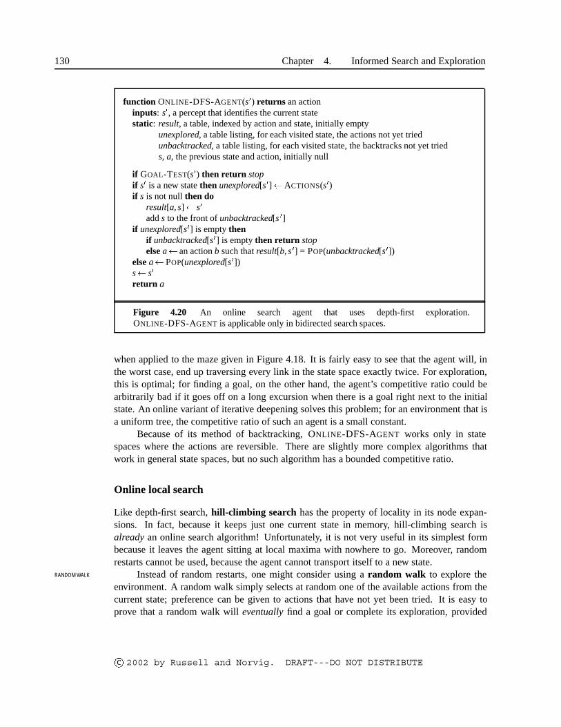
130 Chapter 4. Informed Search and Exploration
function ONLINE-DFS-AGENT(s�) returns an actioninputs: s�, a percept that identifies the current statestatic: result, a table, indexed by action and state, initially empty
unexplored, a table listing, for each visited state, the actions not yet triedunbacktracked, a table listing, for each visited state, the backtracks not yet trieds, a, the previous state and action, initially null
if GOAL-TEST(s�) then return stopif s� is a new state then unexplored[s�]�ACTIONS(s�)if s is not null then do
result[a, s]� s�
add s to the front of unbacktracked[s �]if unexplored[s�] is empty then
if unbacktracked[s�] is empty then return stopelse a� an action b such that result[b, s�] = POP(unbacktracked[s�])
else a� POP(unexplored[s�])s� s�
return a
Figure 4.20 An online search agent that uses depth-first exploration.ONLINE-DFS-AGENT is applicable only in bidirected search spaces.
when applied to the maze given in Figure 4.18. It is fairly easy to see that the agent will, inthe worst case, end up traversing every link in the state space exactly twice. For exploration,this is optimal; for finding a goal, on the other hand, the agent’s competitive ratio could bearbitrarily bad if it goes off on a long excursion when there is a goal right next to the initialstate. An online variant of iterative deepening solves this problem; for an environment that isa uniform tree, the competitive ratio of such an agent is a small constant.
Because of its method of backtracking, ONLINE-DFS-AGENT works only in statespaces where the actions are reversible. There are slightly more complex algorithms thatwork in general state spaces, but no such algorithm has a bounded competitive ratio.
Online local search
Like depth-first search, hill-climbing search has the property of locality in its node expan-sions. In fact, because it keeps just one current state in memory, hill-climbing search isalready an online search algorithm! Unfortunately, it is not very useful in its simplest formbecause it leaves the agent sitting at local maxima with nowhere to go. Moreover, randomrestarts cannot be used, because the agent cannot transport itself to a new state.
Instead of random restarts, one might consider using a random walk to explore theRANDOM WALK
environment. A random walk simply selects at random one of the available actions from thecurrent state; preference can be given to actions that have not yet been tried. It is easy toprove that a random walk will eventually find a goal or complete its exploration, provided
c� 2002 by Russell and Norvig. DRAFT---DO NOT DISTRIBUTE

Section 4.5. Online Search Agents and Unknown Environments 131
that the space is finite.15 On the other hand, the process can be very slow. Figure 4.21 showsan environment in which a random walk will take exponentially many steps to find the goal,because, at each step, backward progress is twice as likely as forward progress. The exampleis contrived, of course, but there are many real-world state spaces whose topology causesthese kinds of “traps” for random walks.
S G
Figure 4.21 An environment in which a random walk will take exponentially many stepsto find the goal.
Augmenting hill climbing with memory rather than randomness turns out to be a moreeffective approach. The basic idea is to store a “current best estimate” ���� of the cost toreach the goal from each state that has been visited. ���� starts out being just the heuristicestimate ���� and is updated as the agent gains experience in the state space. Figure 4.22shows a simple example in a one-dimensional state space. In (a), the agent seems to be stuckin a flat local minimum at the shaded state. Rather than staying where it is, the agent shouldfollow what seems to be the best path to the goal based on the current cost estimates for itsneighbors. The estimated cost to reach the goal through a neighbor �� is the cost to get to�� plus the estimated cost to get to a goal from there—that is, ���� �� ��� � �����. In theexample, there are two actions with estimated costs �� and �� �, so it seems best to moveright. Now, it is clear that the cost estimate of 2 for the shaded state was overly optimistic.Since the best move cost 1 and led to a state that is at least 2 steps from a goal, the shadedstate must be at least 3 steps from a goal, so its � should be updated accordingly, as shownin Figure 4.22(b). Continuing this process, the agent will move back and forth twice more,updating � each time and “flattening out” the local minimum until it escapes to the right.
An agent implementing this scheme, which is called LRTA� (learning, real-time A�), isLRTA*
shown in Figure 4.23. Like ONLINE-DFS-AGENT, it builds a map of the environment usingthe result table. It updates the cost estimate for the state it has just left and then chooses the“apparently best” move according to its current cost estimates. One important detail is thatactions that have not yet been tried in a state � are always assumed to lead immediately to thegoal with the least possible cost, namely ����. This optimism under uncertainty encouragesOPTIMISM UNDER
UNCERTAINTY
the agent to explore new, possibly promising paths.An LRTA� agent is guaranteed to find a goal in any finite, safely explorable environ-
ment. Unlike A�, however, it is not complete for infinite state spaces—there are cases whereit can be led infinitely astray. It can explore an environment of � states in ���� steps inthe worst case, but often does much better. The LRTA� agent is just one of a large family of
�� The infinite case is much more tricky. Random walks are complete on infinite one-dimensional and twodimensional grids, but not on three-dimensional grids! In the latter case, the probability that the walk ever returnsto the starting point is only about 0.3405. (See Hughes, 1995, for a general introduction.)
c� 2002 by Russell and Norvig. DRAFT---DO NOT DISTRIBUTE

132 Chapter 4. Informed Search and Exploration
12
1 11 1 11
1 1 11 1 11
1 1 11 1 11
8 9
8 9
8 9
2
2
3
4
4
4
3
3
3
1 1 11 1 118 9 4 4 3
1 1 11 1 118 9 4 35
3
5
5
4
(a)
(b)
(c)
(d)
(e)
Figure 4.22 Five iterations of LRTA� on a one-dimensional state space. Each state islabeled with �� �, the current cost estimate to reach a goal, and each arc is labeled withits step cost. The shaded state marks the location of the agent, and the updated values arecircled.
function LRTA�-AGENT(s�) returns an actioninputs: s�, a percept that identifies the current statestatic: result, a table, indexed by action and state, initially empty
H, a table of cost estimates indexed by state, initially emptys, a, the previous state and action, initially null
if GOAL-TEST(s�) then return stopif s� is a new state (not in H) then H[s�]��(s�)unless s is null
result[a, s]� s�
H[s]� ����� ACTIONS ���
LRTA�-COST(s, b, result[b, s], H)
a� an action b in ACTIONS(s�) that minimizes LRTA�-COST(s�, b, result[b, s�], H)s� s�
return a
function LRTA�-COST(s, a, s�, H) returns a cost estimateif s� is undefined then return �� �else return �� � �� �� � � ��
Figure 4.23 LRTA�-AGENT selects an action according to the values of neighboringstates, which are updated as the agent moves about the state space.
online agents that can be defined by specifying the action selection rule and the update rulein different ways. We will discuss this family, which was developed originally for stochasticenvironments, in Chapter 19.
Learning in online search
The initial ignorance of online search agents provides several opportunities for learning. First,the agents learn a “map” of the environment—more precisely, the outcome of each action ineach state—simply by recording each of their experiences. (Notice that the assumption of
c� 2002 by Russell and Norvig. DRAFT---DO NOT DISTRIBUTE

Section 4.6. Summary 133
deterministic environments means that one experience is enough for each action.) Second,the local search agents acquire more accurate estimates of the value of each state by usinglocal updating rules, as in LRTA�. In Chapter 19 we will see that these updates eventuallyconverge to exact values for every state, provided that the agent explores the state space in theright way. Once exact values are known, optimal decisions can be taken simply by moving tothe highest-valued successor—that is, pure hill climbing is then an optimal strategy.
If you followed our suggestion to trace the behavior of ONLINE-DFS-AGENT in theenvironment of Figure 4.18, you will have noticed that the agent is not very bright. Forexample, after it has seen that the �� action goes from (1,1) to (1,2), the agent still has noidea that the !"� action goes back to (1,1), or that the �� action also goes from (2,1) to(2,2), from (2,2) to (2,3), and so on. In general, we would like the agent to learn that ��increases the �-coordinate unless there is a wall in the way, that !"� reduces it, and so on.For this to happen, we need two things. First, we need a formal and explicitly manipulablerepresentation for these kinds of general rules; so far, we have hidden the information insidethe black box called the successor function. Part IV is devoted to this issue. Second, we needalgorithms that can construct suitable general rules from the specific observations made bythe agent. These are covered in Chapter 18.
4.6 SUMMARY
This chapter has examined the application of heuristics to reduce search costs. We havelooked at a number of algorithms that use heuristics and found that optimality comes at a stiffprice in terms of search cost, even with good heuristics.
� Best-first search is just GRAPH-SEARCH where the minimum-cost unexpanded nodes(according to some measure) are selected for expansion. Best-first algorithms typicallyuse a heuristic function ���� that estimates the cost of a solution from �.
� Greedy best-first search expands nodes with minimal ����. It is not optimal, but isoften efficient.
� A� search expands nodes with minimal ���� � ���� � ����. A� is complete andoptimal, provided that we guarantee that ���� is admissible (for TREE-SEARCH) orconsistent (for GRAPH-SEARCH). The space complexity of A� is still prohibitive.
� The performance of heuristic search algorithms depends on the quality of the heuris-tic function. Good heuristics can sometimes be constructed by relaxing the problemdefinition, by precomputing solution costs for subproblems in a pattern database, or bylearning from experience with the problem class.
� RBFS and SMA� are robust, optimal search algorithms that use limited amounts ofmemory; given enough time, they can solve problems that A� cannot solve.
� Local search methods such as hill climbing operate on complete-state formulations,keeping only a small number of nodes in memory. Several stochastic algorithms havebeen developed, including simulated annealing, which returns optimal solutions when
c� 2002 by Russell and Norvig. DRAFT---DO NOT DISTRIBUTE

134 Chapter 4. Informed Search and Exploration
given an appropriate cooling schedule. Many local search methods can also be used tosolve problems in continuous spaces.
� A genetic algorithm is a stochastic hill-climbing search in which a large population ofstates is maintained. New states are generated by mutation and by crossover, whichcombines of pairs of states from the population.
� Exploration problems arise when the agent has no idea about the states and actions ofits environment. For safely explorable environments, online search agents can build amap and find a goal if one exists. Updating heuristic estimates from experience providesan effective method to escape from local minima.
BIBLIOGRAPHICAL AND HISTORICAL NOTES
The use of heuristic information in problem solving appears in an early paper by Simonand Newell (1958), but the phrase “heuristic search” and the use of heuristic functions thatestimate the distance to the goal came somewhat later (Newell and Ernst, 1965; Lin, 1965).Doran and Michie (1966) conducted extensive experimental studies of heuristic search asapplied to a number of problems, especially the 8-puzzle and the 15-puzzle. Although Doranand Michie carried out theoretical analyses of path length and “penetrance” (the ratio ofpath length to the total number of nodes examined so far) in heuristic search, they appearto have used their heuristic functions as the sole guiding element in the search, ignoring theinformation provided by current path length. The A� algorithm, incorporating the currentpath length into heuristic search, was developed by Hart, Nilsson, and Raphael (1968), withsome later corrections (Hart et al., 1972). Dechter and Pearl (1985) demonstrated the optimalefficiency of A�.
The original A� paper introduced the consistency condition on heuristic functions. Themonotone condition was introduced by Pohl (1977) as a simpler replacement, but Pearl (1984)showed that the two were equivalent, and now they are used interchangeably. A number of al-gorithms predating A� used the equivalent of open and closed lists; these include breadth-first,depth-first, and uniform-cost search (Bellman, 1957; Ford, 1956; Dijkstra, 1959). Bellman’swork in particular showed the importance of additive path costs in simplifying optimizationalgorithms.
Pohl (1970, 1977) pioneered the study of the relationship between the error in heuris-tic functions and the time complexity of A�. The proof that A� runs in linear time if theerror in the heuristic function is bounded by a constant can be found in Pohl (1977) andin Gaschnig (1979). Pearl (1984) strengthened this result to allow a logarithmic growth inthe error. The “effective branching factor” measure of the efficiency of heuristic search wasproposed by Nilsson (1971).
There are a large number of minor and major variations on the A� algorithm. Pohl (1973)proposed the use of dynamic weighting, which uses a weighted sum �����"����� �"����� of the current path length and the heuristic function as an evaluation function, ratherthan the simple sum ����� ��������� used in A�. The weights "� and "� are adjusted dy-
c� 2002 by Russell and Norvig. DRAFT---DO NOT DISTRIBUTE

Section 4.6. Summary 135
namically as the search progresses. Pohl’s algorithm can be shown to be (-admissible—thatis, guaranteed to find solutions within a factor �� ( of the optimal solution—where ( is a pa-rameter supplied to the algorithm. The same property is exhibited by the A� algorithm (Pearl,1984), which can select any node from the fringe provided its � -cost is within a factor � � (of the lowest-� -cost fringe node. The selection can be done so as to minimize search cost.
A� and other state-space search algorithms are closely related to the branch-and-boundtechniques that are widely used in operations research (Lawler and Wood, 1966). Therelationships between state-space search and branch-and-bound have been investigated indepth (Kumar and Kanal, 1983; Nau et al., 1984; Kumar et al., 1988). Martelli and Monta-nari (1978) demonstrate a connection between dynamic programming (see Chapter 17) andcertain types of state-space search. Kumar and Kanal (1988) attempt a “grand unification” ofheuristic search, dynamic programming, and branch-and-bound techniques under the nameof CDP—the “composite decision process.”
Because computers in the late 1950s and early 1960s had at most a few thousand wordsof main memory, memory-bounded heuristic search was an early research topic. The GraphTraverser (Doran and Michie, 1966), one of the earliest search programs, commits to anoperator after searching best first up to the memory limit. IDA� (Korf, 1985a, 1985b) was thefirst widely used optimal, memory-bounded, heuristic search algorithm, and a large numberof variants have been developed. An analysis of the efficiency of IDA� and of its difficultieswith real-valued heuristics appears in Patrick et al. (1992).
RBFS (Korf, 1991, 1993) is actually somewhat more complicated than the algorithmshown in Figure 4.5, which is closer to an independently developed algorithm called iterativeexpansion, or IE (Russell, 1992). RBFS uses a lower bound as well as the upper bound; theITERATIVE
EXPANSION
two algorithms behave identically with admissible heuristics, but RBFS expands nodes inbest-first order even with an inadmissible heuristic. The idea of keeping track of the bestalternative path appeared earlier in Bratko’s (1986) elegant Prolog implementation of A� andin the DTA� algorithm (Russell and Wefald, 1991). The latter work also discusses metalevelstate spaces and metalevel learning.
The MA� algorithm appeared in Chakrabarti et al. (1989). SMA�, or Simplified MA�,emerged from an attempt to implement MA� as a comparison algorithm for IE (Russell,1992). Kaindl and Khorsand (1994) have applied SMA� to produce a bidirectional search al-gorithm that is substantially faster than previous algorithms. Korf and Zhang (2000) describea divide-and-conquer approach, and Zhou and Hansen (2002) introduce memory-bounded A�
graph search. Korf (1995) surveys memory-bounded search techniques.The idea that admissible heuristics can be derived by problem relaxation appears in the
seminal paper by Held and Karp (1970), who used the the minimum-spanning-tree heuristicto solve the TSP. (See Exercise 4.8.)
The automation of the relaxation process was implemented successfully by Priedi-tis (1993), building on earlier work with Mostow (Mostow and Prieditis, 1989). The useof pattern databases to derive admissible heuristics is due to Gasser (1995) and Culbersonand Schaeffer (1998); disjoint pattern databases are described by Korf and Felner (2002).The probabilistic interpretation of heuristics was investigated in depth by Pearl (1984) andHansson and Mayer (1989).
c� 2002 by Russell and Norvig. DRAFT---DO NOT DISTRIBUTE

136 Chapter 4. Informed Search and Exploration
By far the most comprehensive source on heuristics and heuristic search algorithmsis Pearl’s (1984) Heuristics text. This book provides especially good coverage of the widevariety of offshoots and variations of A�, including rigorous proofs of their formal properties.Kanal and Kumar (1988) present an anthology of important articles on heuristic search. Newresults on search algorithms appear regularly in the journal Artificial Intelligence.
Local-search techniques have a long history in mathematics and computer science. In-deed, the Newton–Raphson method (Newton, 1671; Raphson, 1690) can be seen as a veryefficient local-search method for continuous spaces in which gradient information is avail-able. Brent (1973) is a classic reference for optimization algorithms that do not require suchinformation. Beam search, which we have presented as a local-search algorithm, originatedas a bounded-width variant of dynamic programming for speech recognition in the HARPY
system (Lowerre, 1976). A related algorithm is analyzed in depth by Pearl (1984, Ch. 5).The topic of local search has been reinvigorated in recent years by surprisingly good
results for large constraint satisfaction problems such as �-queens (Minton et al., 1992) andlogical reasoning (Selman et al., 1992) and by the incorporation of randomness, multiplesimultaneous searches, and other improvements. This renaissance of what Christos Papadi-mitriou has called “New Age” algorithms has also sparked increased interest among theoret-ical computer scientists (Koutsoupias and Papadimitriou, 1992; Aldous and Vazirani, 1994).In the field of operations research, a variant of hill climbing called tabu search has gainedTABU SEARCH
popularity (Glover, 1989; Glover and Laguna, 1997). Drawing on models of limited short-term memory in humans, this algorithm maintains a tabu list of � previously visited states thatcannot be revisited; as well as improving efficiency when searching graphs, this can allow thealgorithm to escape from some local minima. Another useful improvement on hill climb-ing is the STAGE algorithm (Boyan and Moore, 1998). The idea is to use the local maximafound by random-restart hill climbing to get an idea of the overall shape of the landscape.The algorithm fits a smooth surface to the set of local maxima and then calculates the globalmaximum of that surface analytically. This becomes the new restart point. The algorithmhas been shown to work in practice on hard problems. (Gomes et al., 1998) showed thatthe run time distributions of systematic backtracking algorithms often have a heavy-taileddistribution, which means that the probability of a very long run time is more than would beHEAVY-TAILED
DISTRIBUTION
predicted if the run times were normally distributed. This provides a theoretical justificationfor random restarts.
Simulated annealing was first described by Kirkpatrick et al. (1983), who borroweddirectly from the Metropolis algorithm (which is used to simulate complex systems inphysics (Metropolis et al., 1953) and was supposedly invented at a Los Alamos dinner party).Simulated annealing is now a subfield in itself, with several hundred papers published everyyear.
Finding optimal solutions in continuous spaces is the subject matter of several fields,including optimization theory, optimal control theory, and the calculus of variations.Suitable (and practical) entry points are provided by Press et al. (2002) and Bishop (1995).Linear programming (LP) was one of the first applications of computers; the simplex algo-rithm (Wood and Dantzig, 1949; Dantzig, 1949) is still used despite worst-case exponentialcomplexity. Karmarkar (1984) developed a practical polynomial-time algorithm for LP.
c� 2002 by Russell and Norvig. DRAFT---DO NOT DISTRIBUTE

Section 4.6. Summary 137
Work by Sewall Wright (1931) on the concept of a fitness landscape was an impor-tant precursor to the development of genetic algorithms. In the 1950s, several statisticians,including Box (1957) and Friedman (1959), used evolutionary techniques for optimizationproblems, but it wasn’t until Rechenberg (1965, 1973) introduced evolution strategies toEVOLUTION
STRATEGIES
solve optimization problems for airfoils that the approach gained popularity. In the 1960sand 1970s, John Holland (1975) championed genetic algorithms, both as a useful tool andas a method to expand our understanding of adaptation, biological or otherwise (Holland,1995). The artificial life movement (Langton, 1995) takes this idea one step further, view-ARTIFICIAL LIFE
ing the products of genetic algorithms as organisms rather than solutions to problems. Workin this field by Hinton and Nowlan (1987) and Ackley and Littman (1991) has done muchto clarify the implications of the Baldwin effect. For general background on evolution, westrongly recommend Smith and Szathmary (1999).
Most comparisons of genetic algorithms to other approaches (especially stochastic hill-climbing) have found that the genetic algorithms are slower to converge, even on problemsspecifically designed to give genetic algorithms an advantage (O’Reilly and Oppacher, 1994;Mitchell et al., 1996; Juels and Wattenberg, 1996; Baluja, 1997). Needless to say, suchfindings are not universally popular within the GA community, but recent attempts withinthat community to understand population-based search as an approximate form of Bayesianlearning (see Chapter 18) might help to close the gap between the field and its critics (Pelikanet al., 1999). The theory of quadratic dynamical systems may also explain the performanceof GAs (Rabani et al., 1998). See Lohn et al. (2001) for an example of GAs applied toantenna design, and Larranaga et al. (1999) for an application to the travelling salespersonproblem.
The field of genetic programming is closely related to genetic algorithms. The princi-GENETICPROGRAMMING
pal difference is that the representations that are mutated and combined are programs ratherthan bit strings. The programs are represented in the form of expression trees; the expressionscan be in a standard language such as Lisp or can be specially designed to represent circuits,robot controllers, and so on. Crossover involves splicing together subtrees rather than sub-strings. This form of mutation guarantees that the offspring are well-formed expressions,which would not be the case if programs were manipulated as strings.
Recent interest in genetic programming was spurred by John Koza’s work (Koza, 1992,1994), but it goes back at least to early experiments with machine code by Friedberg (1958)and with finite-state automata by Fogel et al. (1966). As with genetic algorithms, there isdebate about the effectiveness of the technique. Koza et al. (1999) describe a variety ofexperiments on the automated design of circuit devices using genetic programming.
The journals Evolutionary Computation and IEEE Transactions on Evolutionary Com-putation cover genetic algorithms and genetic programming; articles are also found in Com-plex Systems, Adaptive Behavior, and Artificial Life. The main conferences are the Inter-national Conference on Genetic Algorithms and the Conference on Genetic Programming,recently merged to form the Genetic and Evolutionary Computation Conference. The textsby Melanie Mitchell (1996) and David Fogel (2000) give good overviews of the field.
Algorithms for exploring unknown state spaces have been of interest for many centuries.Depth-first search in a maze can be implemented by keeping one’s left hand on the wall; loops
c� 2002 by Russell and Norvig. DRAFT---DO NOT DISTRIBUTE

138 Chapter 4. Informed Search and Exploration
can be avoided by marking each junction. Depth-first search fails with irreversible actions; themore general problem of exploring of Eulerian graphs (i.e., graphs in which each node hasEULERIAN GRAPHS
equal numbers of incoming and outgoing edges) was solved by an algorithm due to Hierholzer(1873). The first thorough algorithmic study of the exploration problem for arbitrary graphswas carried out by Deng and Papadimitriou (1990), who developed a completely generalalgorithm, but showed that no bounded competitive ratio is possible for exploring a generalgraph. Papadimitriou and Yannakakis (1991) examined the question of finding paths to a goalin geometric path-planning environments (where all actions are reversible). They showed thata small competitive ratio is achievable with square obstacles, but with general rectangularobstacles no bounded ratio can be achieved. (See Figure 4.19.)
The LRTA� algorithm was developed by Korf (1990) as part of an investigation intoreal-time search for environments in which the agent must act after searching for only aREAL-TIME SEARCH
fixed amount of time (a much more common situation in two-player games). LRTA� is infact a special case of reinforcement learning algorithms for stochastic environments (Bartoet al., 1995). Its policy of optimism under uncertainty—always head for the closest unvisitedstate—can result in an exploration pattern that is less efficient in the uninformed case thansimple depth-first search (Koenig, 2000). Dasgupta et al. (1994) show that online iterativedeepening search is optimally efficient for finding a goal in a uniform tree with no heuristicinformation. Several informed variants on the LRTA� theme have been developed with dif-ferent methods for searching and updating within the known portion of the graph (Pembertonand Korf, 1992). As yet, there is no good understanding of how to find goals with optimalefficiency when using heuristic information.
The topic of parallel search algorithms was not covered in the chapter, partly becausePARALLEL SEARCH
it requires a lengthy discussion of parallel architectures. As parallel computers are becomingwidely available, parallel search is becoming an important topic in both AI and theoreticalcomputer science. A brief introduction to the AI literature can be found in Mahanti andDaniels (1993).
EXERCISES
4.1 Trace the operation of A� search applied to the problem of getting to Bucharest fromLugoj using the straight-line distance heuristic. That is, show the sequence of nodes that thealgorithm will consider and the � , �, and � score for each node.
4.2 The heuristic path algorithm is a best-first search in which the objective function is���� � �� � "����� � "����. For what values of " is this algorithm guaranteed to beoptimal? What kind of search does this perform when " � �? When " � �? When" � �?
4.3 Prove each of the following statements:
a. Breadth-first search is a special case of uniform-cost search.
c� 2002 by Russell and Norvig. DRAFT---DO NOT DISTRIBUTE

Section 4.6. Summary 139
b. Breadth-first search, depth-first search, and uniform-cost search are special cases ofbest-first search.
c. Uniform-cost search is a special case of A� search.
4.4 Devise a state space in which A� using GRAPH-SEARCH returns a suboptimal solutionwith an ���� function that is admissible but inconsistent.
4.5 We saw on page 101 that the straight-line distance heuristic leads greedy best-firstsearch astray on the problem of going from Iasi to Fagaras. However, the heuristic is per-fect on the opposite problem: going from Fagaras to Iasi. Are there problems for which theheuristic is misleading in both directions?
4.6 Invent a heuristic function for the 8-puzzle that sometimes overestimates, and showhow it can lead to a suboptimal solution on a particular problem. (You can use a computer tohelp if you want.) Prove that, if � never overestimates by more than �, A� using � returns asolution whose cost exceeds that of the optimal solution by no more than �.
4.7 Prove that if a heuristic is consistent, it must be admissible. Construct an admissibleheuristic that is not consistent.
4.8 The travelling- salesperson problem (TSP) can be solved via the minimum spanningtree (MST) heuristic, which is used to estimate the cost of completing a tour, given that apartial tour has already been constructed. The MST cost of a set of cities is the smallest sumof the link costs of any tree that connects all the cities.
a. Show how this heuristic can be derived from a relaxed version of the TSP.
b. Show that the MST heuristic dominates straight-line distance.
c. Write a problem generator for instances of the TSP where cities are represented byrandom points in the unit square.
d. Find an efficient algorithm in the literature for constructing the MST, and use it with anadmissible search algorithm to solve instances of the TSP.
4.9 On page 112, we defined the relaxation of the 8-puzzle in which a tile can move fromsquare A to square B if B is blank. The exact solution of this problem defines Gaschnig’sheuristic (Gaschnig, 1979). Explain why Gaschnig’s heuristic is at least as accurate as ��(misplaced tiles), and show cases where it is more accurate than both �� and �� (Manhattandistance). Can you suggest a way to calculate Gaschnig’s heuristic efficiently?
4.10 We gave two simple heuristics for the 8-puzzle: Manhattan distance and misplacedtiles. Several heuristics in the literature purport to improve on Manhattan distance—see,for example, Nilsson (1971), Mostow and Prieditis (1989), and Hansson et al. (1992). Testthese claims by implementing the heuristics and comparing the performance of the resultingalgorithms.
4.11 Give the name of the algorithm that results from each of the following special cases:
a. Local beam search with � � �.
b. Local beam search with � ��.
c� 2002 by Russell and Norvig. DRAFT---DO NOT DISTRIBUTE

140 Chapter 4. Informed Search and Exploration
c. Simulated annealing with ) � � at all times.d. Genetic algorithm with population size � � �.
4.12 Sometimes there is no good evaluation function for a problem, but there is a goodcomparison method: a way to tell whether one node is better than another, without assigningnumerical values to either. Show that this is enough to do a best-first search. Is there ananalogue of A�?
4.13 Relate the time complexity of LRTA� to its space complexity.
4.14 Suppose that an agent is in a � � maze environment like the one shown in Fig-ure 4.18. The agent knows that its initial location is (1,1), that the goal is at (3,3), and that thefour actions ��, !"�, *$�', +,��' have their usual effects unless blocked by a wall. Theagent does not know where the internal walls are. In any given state, the agent perceives theset of legal actions; it can also tell whether the state is one it has visited before or a new state.
a. Explain how this online search problem can be reconceptualized as an offline searchin belief state space, where the initial belief state includes all possible environmentconfigurations. How large is the initial belief state? How large is the space of beliefstates?
b. How many distinct percepts are possible in the initial state?c. Describe the first few branches of a contingency plan for this problem. How large
(roughly) is the complete plan?
Notice that this contingency plan is a solution for every possible environment fitting the givendescription. Therefore, interleaving of search and execution is not strictly necessary even inunknown environments.
4.15 (a) Devise a hill-climbing approach to solve travelling salesperson problems. Comparethe results with optimal solutions obtained via the A� and the MST heuristic (Exercise 4.8).(b) Devise a genetic algorithm approach to the travelling salesperson problem. Compareresults to the other approaches. You may want to consult Larranaga et al. (1999) for somesuggestions for representations.
4.16 Generate a large number of 8-puzzle and 8-queens instances and solve them (wherepossible) by hill climbing (steepest-ascent and first-choice variants), hill climbing with ran-dom restart, and simulated annealing. Measure the search cost and percentage of solvedproblems and graph these against the optimal solution cost. Comment on your results.
4.17 In this exercise, we will examine hill climbing in the context of robot navigation, usingthe environment in Figure 3.22 as an example.
a. Repeat Exercise 3.16 using hill climbing. Does your agent ever get stuck in a localminimum? Is it possible for it to get stuck with convex obstacles?
b. Construct a nonconvex polygonal environment in which the agent gets stuck.c. Modify the hill-climbing algorithm so that, instead of doing a depth-1 search to decide
where to go next, it does a depth-� search. It should find the best �-step path and doone step along it, and then repeat the process.
c� 2002 by Russell and Norvig. DRAFT---DO NOT DISTRIBUTE

Section 4.6. Summary 141
d. Is there some � for which the new algorithm is guaranteed to escape from local minima?
e. Explain how LRTA� enables the agent to escape from local minima in this case.
4.18 Compare the performance of A� and RBFS on a set of randomly generated problemsin the 8-puzzle (with Manhattan distance) and TSP (with MST—see Exercise 4.8) domains.Discuss your results. What happens to the performance of RBFS when a small random num-ber is added to the heuristic values in the 8-puzzle domain?
c� 2002 by Russell and Norvig. DRAFT---DO NOT DISTRIBUTE