Solution Spaces for Linear Equations in Valued...

Solution Spaces for Linear Equations in Valued D-Fields

by

Meghan Anderson

A dissertation submitted in partial satisfaction of the

requirements for the degree of

Doctor of Philosophy

in

Mathematics

in the

Graduate Division

of the

University of California, Berkeley

Committee in charge:

Professor Thomas Scanlon, ChairProfessor Leo A. Harrington

Professor Paolo Mancosu

Spring 2011


Copyright 2011by

Meghan Anderson

1

Abstract


by

Meghan Anderson

Doctor of Philosophy in Mathematics

University of California, Berkeley

Professor Thomas Scanlon, Chair

In his 1997 thesis, Thomas Scanlon developed the model theory of a class of valuedfields, which allow for the consideration of a difference field and a related differential fieldin the same structure. In this theory, fields are endowed with a derivative like operator D,interacting strongly with a valuation. The operator specializes to a derivative in the residuefield, but in the valued field is interdefinable with a nontrivial automorphism. The theorywas shown to have good model theoretic properties, most notably quantifier elimination.

We look at solutions to linear D-equations in these fields, with the goal of using the residuedifferential field to better understand the behavior of the difference field solutions. First, weshow that the dimension of a maximal solution space to such an equation as a vector spaceover the constants is completely determined by the structure induced on the residue field.We then find reasonable conditions on the base field sufficient to assure uniqueness for thefield extension generated by these solutions. Finally, we provide examples of automorphismgroups in the theory; in particular, we show that nonlinear relations in the residue field maynot lift to the valued field.

i

Contents

1 Introduction 1

1.1 Motivation . . . . . . . . . . . . . . . . . . . . . . . . . . . . . . . . . . . . . . . . . 1

2 Preliminaries 3

2.1 Differential Algebra . . . . . . . . . . . . . . . . . . . . . . . . . . . . . . . . . . . 32.2 Differential Galois Theory . . . . . . . . . . . . . . . . . . . . . . . . . . . . . . . 62.3 Difference Fields . . . . . . . . . . . . . . . . . . . . . . . . . . . . . . . . . . . . . 82.4 Model Theoretic View . . . . . . . . . . . . . . . . . . . . . . . . . . . . . . . . . . 9

3 Valued D-fields 11

3.1 De-Rings . . . . . . . . . . . . . . . . . . . . . . . . . . . . . . . . . . . . . . . . . . 113.2 Valued Fields . . . . . . . . . . . . . . . . . . . . . . . . . . . . . . . . . . . . . . . 133.3 �VDF: Axioms and Consequences . . . . . . . . . . . . . . . . . . . . . . . . . . . 153.4 Algebra in Valued D-Fields . . . . . . . . . . . . . . . . . . . . . . . . . . . . . . . 18

4 Solutions to Linear D-Equations 22

4.1 Valuation Compatibility . . . . . . . . . . . . . . . . . . . . . . . . . . . . . . . . . 224.2 D-fundamental systems of solutions . . . . . . . . . . . . . . . . . . . . . . . . . . 27

5 Galois Theory 28

5.1 PVD-extensions . . . . . . . . . . . . . . . . . . . . . . . . . . . . . . . . . . . . . . 285.2 Liaison Groups . . . . . . . . . . . . . . . . . . . . . . . . . . . . . . . . . . . . . . 30

6 Examples 32

6.1 Maximality of Constants . . . . . . . . . . . . . . . . . . . . . . . . . . . . . . . . 326.2 Fixed Fields and Imaginaries . . . . . . . . . . . . . . . . . . . . . . . . . . . . . . 336.3 Definability . . . . . . . . . . . . . . . . . . . . . . . . . . . . . . . . . . . . . . . . 346.4 Vector Space Dimension . . . . . . . . . . . . . . . . . . . . . . . . . . . . . . . . . 366.5 Algebraic Relations . . . . . . . . . . . . . . . . . . . . . . . . . . . . . . . . . . . 40

Bibliography 44

1

Chapter 1

Introduction

1.1 Motivation

A model complete theory of valued D-fields, called �VDF, was developed by Scanlon in [18].In this theory, the fields are endowed with a additive operator D, interacting in a naturalway with the valuation. The D-operator specializes to a derivation in the residue field, butin the valued field but obeys a twisted Leibniz rule:

D(xy) = xD y + y Dx + εDxD y

where ε is a fixed element of positive valuation. Such a D-operator is interdefinable withan automorphism σ of the valued field, defined by σ(x) ∶= x + εDx. Additional axioms,notably one demanding that there are D-constants at every valuation and that an analogueof Hensel’s lemma holds, assure that the theory has quantifier elimination.

This setting should allow for some information from the well understood differential fieldsdownstairs to be lifted to the more complicated difference fields upstairs. This analysis isfeasible thanks to the good model theoretic properties of �VDF, in particular the aforemen-tioned quantifier elimination. However, the theory also presents its own challenges, evenin the relatively simple setting of solution spaces to linear equations. This thesis addressessome of these challenges and begins work on such an analysis.

The first difficulty arises from the fact that not all difference field extensions are compat-ible with the axioms for �VDF. Therefore, it may not always be possible to adjoin as manysolutions to a given equation as one would like, and the solution spaces to linear differenceequations will often be strictly smaller than those traditionally considered. Furthermore,while it is easy to see that the axioms �VDF will have an effect on solution space size, itrequires some work to see exactly what this effect will be.

In Chapter 4, we show that dimension of the solutions space to a linear D-equation in�VDF depends in a strong and systematic way on the structure induced on the residue field.With this result, what was once a complication can now be considered a feature of the theory,

2

as it allows for further distinctions about the structure of the solutions to D-equations thanare possible purely algebraically.

A second hurdle is the fact that it is not known whether �VDF has prime models. Thus, it isnot immediately obvious that the extension generated by a maximal set of solutions to a linearD-equation will be unique. In Chapter 5, we will show that with reasonable assumptions onthe constants of the base field, these extensions are unique up to isomorphism. We will alsodemonstrate the necessity of these assumptions by exhibiting an example where, withoutthem, the desired uniqueness result fails.

These two elements allow for a meaningful model theoretic Galois theory, outlined at theend of Chapter 5. In Chapter 6, we take a closer look at both sides of this correspondenceby working through several examples.

3

Chapter 2

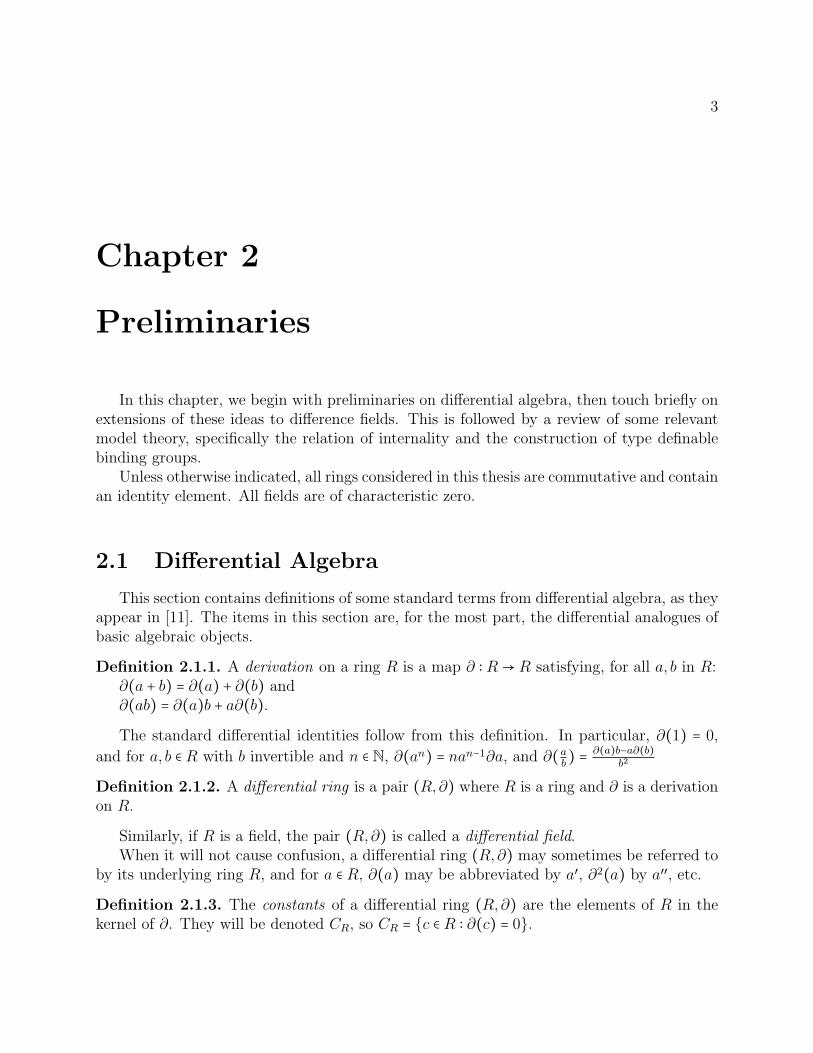
Preliminaries

In this chapter, we begin with preliminaries on differential algebra, then touch briefly onextensions of these ideas to difference fields. This is followed by a review of some relevantmodel theory, specifically the relation of internality and the construction of type definablebinding groups.

Unless otherwise indicated, all rings considered in this thesis are commutative and containan identity element. All fields are of characteristic zero.

2.1 Differential Algebra

This section contains definitions of some standard terms from differential algebra, as theyappear in [11]. The items in this section are, for the most part, the differential analogues ofbasic algebraic objects.

Definition 2.1.1. A derivation on a ring R is a map ∂ ∶ R → R satisfying, for all a, b in R:∂(a + b) = ∂(a) + ∂(b) and∂(ab) = ∂(a)b + a∂(b).

The standard differential identities follow from this definition. In particular, ∂(1) = 0,and for a, b ∈ R with b invertible and n ∈ N, ∂(an) = nan−1∂a, and ∂(

ab ) =

∂(a)b−a∂(b)b2

Definition 2.1.2. A differential ring is a pair (R,∂) where R is a ring and ∂ is a derivationon R.

Similarly, if R is a field, the pair (R,∂) is called a differential field.When it will not cause confusion, a differential ring (R,∂) may sometimes be referred to

by its underlying ring R, and for a ∈ R, ∂(a) may be abbreviated by a′, ∂2(a) by a′′, etc.

Definition 2.1.3. The constants of a differential ring (R,∂) are the elements of R in thekernel of ∂. They will be denoted CR, so CR = {c ∈ R ∶ ∂(c) = 0}.

4

Equivalently, c ∈ CR if for all a ∈ R, ∂(ca) = c∂(a). The constants of a differential ringform a ring, and the constants of a differential field form a field.

Proposition 2.1.4. If R is a differential ring, and a ∈ R is algebraic over CR, then a ∈ CR.

Proof. Let P (x) = ∑ni=0 cix

i be a minimal polynomial for a over CR. Since P (a) = 0,

D(P (a)) = �

n

�i=1

ci(i)ai−1�∂(a) = 0

So either ∂(a) = 0 or (∑ni=1 ci(i)a

i−1) = 0, contradicting the minimality of P .

Definition 2.1.5. A differential ring (S,∂S) is a differential extension of (R,∂R) if S is anextension of R as a ring, and for all a ∈ R, ∂S(a) = ∂R(a).

Definition 2.1.6. A differential homomorphism from (R,∂R) to (S,∂S) is a ring homomor-phism φ ∶ R → S making the following diagram commute:

Rφ

��→ S

��

∂R

��

∂S

Rφ

��→ S

Definition 2.1.7. A differential ideal I of (R,∂) is an ideal of R such that ∂(I) ⊆ I.

If I is an ideal of a differential ring (R,∂), then ∂ induces the structure of a differentialring on R�I exactly when I is a differential ideal.

Definition 2.1.8. A simple differential ring is a differential ring whose only differentialideals are (0) and R.

A simple differential ring need not be simple as a ring. For example, zC[z] is up anontrivial ring ideal in C[z], but are not closed under the derivation ∂ =

ddz . In fact, no

nontrivial ideals in (C[z], ddz) are closed under d

dz , making (C[z], ddz) a simple differential

ring.

Definition 2.1.9. A differential algebra over (R,∂R) is a differential ring (S,∂S) giventogether with a homomorphism of differential rings (R,∂R)→ (S,∂S).

Definition 2.1.10. The tensor product of two differential algebras, (T,∂T ) and (S,∂S), overa differential ring R is the ring T ⊗R S, with ∂T⊗RS defined for t ∈ T and s ∈ S by,

∂T⊗RS(t⊗R s) = (∂T (t)⊗R s) + (t⊗R ∂S(s)).

5

To that the map ∂T⊗RS is a well defined derivation, check first the case where the deriva-tion on R is trivial. For general R, observe that T ⊗R S is the quotient of T ⊗C S by the ringideal I generated by elements of the form {1⊗C 1.r − r.1⊗C 1} for r ∈ R, and that this I is adifferential ideal.

Definition 2.1.11. For a differential ring R, R{X} is the ring of differential polynomials

over R in the variable X. It is the ring of polynomials in countably many variables

R{X} ∶= R[X,X′,X′′, . . . ,X

(n), . . .]

with the derivation on R extended so that ∂(X(n)) =X(n+1).A differential polynomial can be considered as a differential operator, via the map

R{X}→ End(R) that takes X(n) to ∂nR and a ∈ R to left multiplication by a.

Given a differential ring (R,∂R) and a multiplicative subset S ⊆ R, we can consider thelocalization S−1R. As usual, the elements are classes of ordered pairs (r, s) where r ∈ R ands ∈ S modulo the equivalence relation dened by (r1, s1) ∼ (r2, s2) if there is some t ∈ S witht(s2r1 − s1r2) = 0. This localization S−1R can be given the structure of a differential ring.

Proposition 2.1.12. Given a differential ring (R,∂R) and a S a multiplicative subset of R,

∂R extendes uniquely to S−1R by the quotient rule ∂(r, s) = (s∂r − r∂s, s2).

Proof. It is clear that if ∂R extends to S−1R, it must obey the quotient rule, so if an extensionexists, it is unique.

For this extension to be well defined, it must preserve the equivalence classes that makeup S−1R. Thus, the derivation will preserve equivalence classes if whenever there is somet ∈ R such that

t(r1s2 − r2s1) = 0

there is also a t∗ ∈ R such that

t∗�(∂(r1)s1 − r1∂(s1))s

22 − (∂(r2)s2 − r2∂(s2))s

21� = 0.

A straightforward verification shows that t2 is such a t∗.

Proposition 2.1.13. If (F,∂F ) is a differential field (of characteristic 0), then ∂F extends

uniquely to the algebraic closure F of F .

Proof. To see that the derivation extends uniquely to any finite extension,Suppose a ∈ F �F and let P (x) = ∑

ni=0 fix

i be its minimal polynomial over F with f1 = 1,and using the primitive element theorem suppose further that a is a primitive root of P , soP (x) splits in F (a).

6

Now suppose we have extended the derivation ∂F to a derivation ∂ on all of F (a). Byapplying this ∂ to the minimal polynomial, we can solve for ∂(a) in terms of a and elementsin F . Any element in F (a) is an F linear combination of {1, a, a2, . . . an−1}, and for any suchlinear combination, b ∶= ∑

ni=0 fia

i, ∂b can be computed in terms of this ∂a, so if the derivationcan be extended, it is unique.

To see that this gives a valid derivation, one checks that for b1, b2 ∈ K(a), the Leibnizrule

∂(b1b2) = b1∂b2 + b2∂b1

holds, which reduces to to showing that ∂(ak) = kak−1∂(a) for n ≤ k ≤ 2n − 1. This can bedone by induction, making use of the minimal polynomial for a.

Since F is the union of F (a) over all such a, we see that ∂F has a unique extension to F .

2.2 Differential Galois Theory

Differential Galois theory is the study of the differential field extensions generated tosolutions to differential equations and of their automorphism groups. Here, we recall someof the basic ideas and definitions from the differential Galois theory of linear differentialequations. An excellent introduction can be found in [11], which we continue to follow here;for a more exhaustive reference, turn to [21].

If L is an order n linear differential operator over a differential field F , then the solutionsto the equation L = 0 will form a vector space over the constants of dimension at most n.Furthermore, there is some differential extension K ⊇ F in which L = 0 has n solutions,linearly independent over the constants of K. If {f1 . . . fn} is a set of n solutions to L = 0in a differential field K, linearly independent over the constants of K, then {f1 . . . fn} is afundamental system of solutions of L in K.

If K ⊇ F is a differential field extension and the constants of K are the constants of F ,then K is a no new constants extension of F . If CF is algebraically closed, then for any L

over F , there is a K ⊇ F containing a fundamental system of solutions to L with CK = CF .Such extensions are called Picard-Vessiot extensions; they are the smallest differential fieldextensions containing a full set of solutions to a given equation.

The assumption that CF be algebraically closed is relatively benign, as the derivation onany differential field extends uniquely to its algebraic closure by Proposition 2.1.13 and theconstants of an algebraically closed differential field will themselves be algebraically closedby Proposition 2.1.4.

Definition 2.2.1. Let (F,∂) be a differential field and L, a linear differential operator oforder n over K. A Picard-Vessiot extension of F for L is a differential extension F ⊆K suchthat:

7

1. The constants of K are the constants of F ,

2. L = 0 has n solutions in K linearly independent over these constants

3. K is generated over F as a differential field by the solutions of L = 0 in K.

An order n linear differential equation can also be written as ∂(x) = Ax, where A ∈

Gln(K), x is a vector, and ∂ acts on x component-wise. We say that M is a fundamental

matrix for the equation ∂(x) = Ax if M is an invertible matrix satisfying ∂(M) = AM . APicard-Vessiot extension can then be equivalently defined as a no new constants extensionof F generated as a field by the entries of M .

If the constants of F are algebraically closed, then any two Picard Vessiot extensions ofF for L are isomorphic over F as differential fields.

Picard Vessiot extensions play the role of Galois extensions in differential Galois theory.

Let Aut(K�F ) be the group of field automorphisms of K over F ; it is a subgroup ofGLn(CK). Let DGal(K/F) be the group of differential automorphisms of K over F ; that is,the subgroup of Aut(K�F ) of elements σ such that for all a ∈ K, ∂(σ(a)) = σ(∂(a)). ThenDGal(K/F), considered as a subgroup of GLn(CK), is an algebraic group. Furthermore, itcan be shown using Proposition 2.1.13 that any finite Galois extension of K ⊇ F is a PicardVessiot extension for some equation, and that in this case the differential Galois group willbe the same as the ordinary Galois group of the extension.

For a Picard Vessiot extension K ⊇ F , there is a Galois correspondence between inter-mediate differential field extensions and subgroups of DGal(K�F ).

Theorem 2.2.2 (Fundamental Theorem of Differential Galois Theory). Let K ⊇ F be a

Picard Vessiot Extension, and set G ∶= DGal(K�F ). Then there is a lattice inverting bijective

correspondence:

{differential subfields F ⊆ E ⊆K}↔ {Zariski closed subgroups H of G}

given by:

E → {elements in G fixing E}

{the fixed field of H}←H

with Picard Vessiot extensions corresponding to normal subgroups.

While we will consider only linear equations in this thesis, it is worth noting that Kolchindeveloped a differential Galois theory for a wider class of equations. The extensions consid-ered are called strongly normal.

Definition 2.2.3. Let K and L be differential fields with K ⊆ L, both inside a universaldifferential field U . The extensions L�K is strongly normal if and only if:

8

1. CK = CL is algebraically closed;

2. L is finitely generated over K

3. if σ ∶ U → U is a differential automorphism fixing K pointwise, then �L,CU� = �σ(L),CU�.Picard Vessiot extensions are strongly normal, but certain nonlinear differential equations

also give rise to strongly normal extensions, and can therefore be shown to have a good Galoistheory.

2.3 Difference Fields

A difference ring (R,σ) is ring R together with a ring automorphism σ ∶ R → R. Theconstants of R are the elements c ∈ R with σ(c) = c, and are denoted CR. A difference ringthat is a field is a difference field. When working in a difference ring, the image of x ∈ R

under the automorphism σ is sometimes denoted σ(x), and sometimes xσ.A Galois theory of linear difference equations has been developed in analogy with dif-

ferential Galois theory; a good reference on the subject is [20]. A fundamental system ofsolutions for an order n linear equation L(x) = 0 over a difference field F is again a set of n

solutions to the equation in K ⊇ F , linearly independent over the constants of K. If K is ano new constants extension of F , generated by such a fundamental system of solutions, K

is again called a Picard Vessiot extension of F for L. If the constants of F are algebraicallyclosed, such a K exists and is unique up to isomorphism over F , and the expected Galoiscorrespondence holds.

However, in difference fields, the requirement that the constants be algebraically closedis a significant restriction. A difference field (F,σ) might contain nonconstant elementsalgebraic over CF , and σ might not have a unique extension to the algebraic closure of F .One consequence of this is that some equations may never have any nonzero solutions in adifference field with algebraically closed constants. The simplest example of such an equationis σ(x) = −x. Since the square of any solution is a constant, any nonzero solution will be anonconstant element algebraic over the constants.

The Galois theory of difference equations has therefore been expanded in multiple direc-tions. In order to include equations like σ(x) = −x, one can consider field extensions whosefields of constants are not algebraically closed, or Picard Vessiot rings that are not neces-sarily integral (a solution to σ(x) = x in such a ring would also satisfy x2 = 0). A survey ofthese is given in [3], where it is also proved that in the cases they coincide, three reasonableapproaches lead to essentially the same Galois theory.

An algorithm for computing the Galois group of an order two difference equation over(K,σ), for K = k(z), where k is a finite algebraic extension of Q and σ(z) = z + 1 is givenin [6]. We will use this algorithm in the examples, in order to compare model theoretic

9

automorphism groups in valued D-fields to the standard difference Galois groups for thesame equations.

To a second order linear difference equation σ2x + aσx + bx = 0, the procedure associatesa first order nonlinear difference equation xσx+ ax+ b = 0 called the Riccati equation. If theRiccati equation has a solution u in the base field, then the difference operator σ2 + aσ + b

factors as (σ− bu)(σ−u). The algorithm draws the following conclusions about the difference

Galois group G based on the number of solutions to the Riccati equation in K ∶= (Q(t)).

1. If the Riccati equation has no solutions in K, then G is irreducible.

2. If the Riccati equation has exactly one solution u in K, then G is reducible, but notcompletely reducible.

3. If the Riccati equation has exactly two solutions u1 and u2 in K then G is completelyreducible, but not an algebraic subgroup of {c.Id ∶ c ∈ Q×}.

4. If the Riccati equation more than two solutions, then G is an algebraic subgroup of{c.Id ∶ c ∈ Q×}.

In the cases we encounter, the Riccati equation will have two solutions. It is also shownin [6] that if G0 is the identity component of G, and G is a reducible difference Galois groupin this setting, then G�G0 is finite cyclic. Thus, the problem is reduced to considering suchreducible subgroups of GL(2,CK). This can be done by inspection, as the subgroup mustcontain the matrix

�u1 00 u2

�

corresponding to equation in its factored form.

2.4 Model Theoretic View

There is also a model theoretic Galois theory, which in its most basic form relates defin-ably closed sets in some model with (quotients of) groups of automorphisms of that model.We introduce this Galois theory here; for basic model theoretic definition and concepts, see[13], [7], or [17].

For two definable sets Q and C in some model U , the model theoretic Galois groupMGal ∶= Aut(Q�C)(U) of Q over C in U is the group of automorphisms of Q induced byautomorphisms of U fixing C pointwise. If Q is internal to C; meaning there is some finitetuple b such that in any model, the elements of Q are definable over Cb, this automorphismgroup is type definable. When Q and C are definably closed, and Th(U) eliminates imag-inaries, there is a Galois correspondence between type definable subgroups of MGal anddefinably closed substructures S of U with C ⊆ S ⊆Q.

10

An excellent introduction to the subject is the recent [14], while a complete technicaltreatment with minimal assumptions on the theory is given in [8]. A detailed look at the“internality” relation and exhaustive treatment of the Galois correspondence is given in [9].

In the early 1980’s, the connection between these model theoretic automorphism groupsand differential galois theory was noted in [16]. Later, this connection was more fully devel-oped by Pillay in [15], which uses the model theoretic framework to generalize the Kolchintheory. The setting for this work is DCF0, the theory of differentially closed fields of charac-teristic zero. These universal differential fields were described in the 1950’s by Kolchin andRobinson, and later shown to have the following finite axiomatization by Lenore Blum.

Definition 2.4.1. A differential field K is differentially closed if for all f, g ∈ K{X}, withorder(f)>order(g), there is some x ∈K with f(x) = 0 and g(x) ≠ 0.

Differentially closed fields are the subject of [12]. Any differential field of characteristiczero embeds into a model of DCF0. The theory has quantifier elimination, is complete andω-stable, and eliminates imaginaries.

Using these facts, we can uniquely associate to any linear differential equation L over adifferential field K the set QL of solutions to L in a prime modelM of DCF0 over K. If C

is the set of constants, then QL is C-internal; QL is a finite dimensional vector space overC, if b is a basis for QL over C every element of Q is definable over Cb. The model theoreticGalois group of QL over C inM is therefore type definable.

By ω-stability, any type definable group in DCF0 is in fact definable. Furthermore, onecan identify the model theoretic Galois group in DCF0 with the standard differential Galoisgroup associated to L. The construction of the group used the fact that L was a linearequation only in establishing that QL was C internal; everything above makes sense inDCF0 for any sets Q and C satisfying the internality relation. This can be shown to includeany case where C is the set of constants and the extension generated by Q is a stronglynormal extension of the base field.

11

Chapter 3

Valued D-fields

3.1 De-Rings

Everything in this section comes directly from [18]. For ease of reference, throughoutthis section and the two that follow, we retain the notation of that paper.

Let L be the language of rings, along with an extra function symbol D and a constant e.

Definition 3.1.1. A De-ring is an L-structure R such that

● R is a ring,

● e some element in R, and

● D is a additive map from R to R, satisfying D(1) = 0 and the twisted Leibniz ruleD(xy) =D(x)y + xD(y) + eD(x)D(y).

Given D, we can define an endomorphism σ of R by the formula σ(x) ∶= x + eDx, andthe twisted Leibniz rule can be rewritten as D(xy) = xDy + σ(y)Dx.

The definition above makes sense for any ring R and any e ∈ R, but there are somespecial cases. If e = 0, there is no twisting, σ = id and D is a derivation. If e ≠ 0, σ isa nontrivial endomorphism, and this twisting means that D operator can no longer be aderivation. Furthermore, if e is not a zero divisor, then σ and D are interdefinable, and D

can be recovered from σ by eD(x) = (σ(x) − x), making (R,D) equivalent to the differencering (R,σ). When e is invertible, the situation is recognizable as that of a σ-derivation,δσ(x) ∶= γ(xσ − x) with γ = e−1. Modules over rings with such an operator are deeplyexplored in [1].

Many facts familiar from differential algebra remain true in the D-ring setting. Theconstants of a D-ring form a ring, and the constants of a D-field form a field. D-extensionsand D-algebras are defined in the expected way. If R is a D-ring and I ⊆ R is an ideal, wesay I is a D-ideal if D(I) ⊆ I, in which case the structure induced on R�I is also that of aD-ring.

12

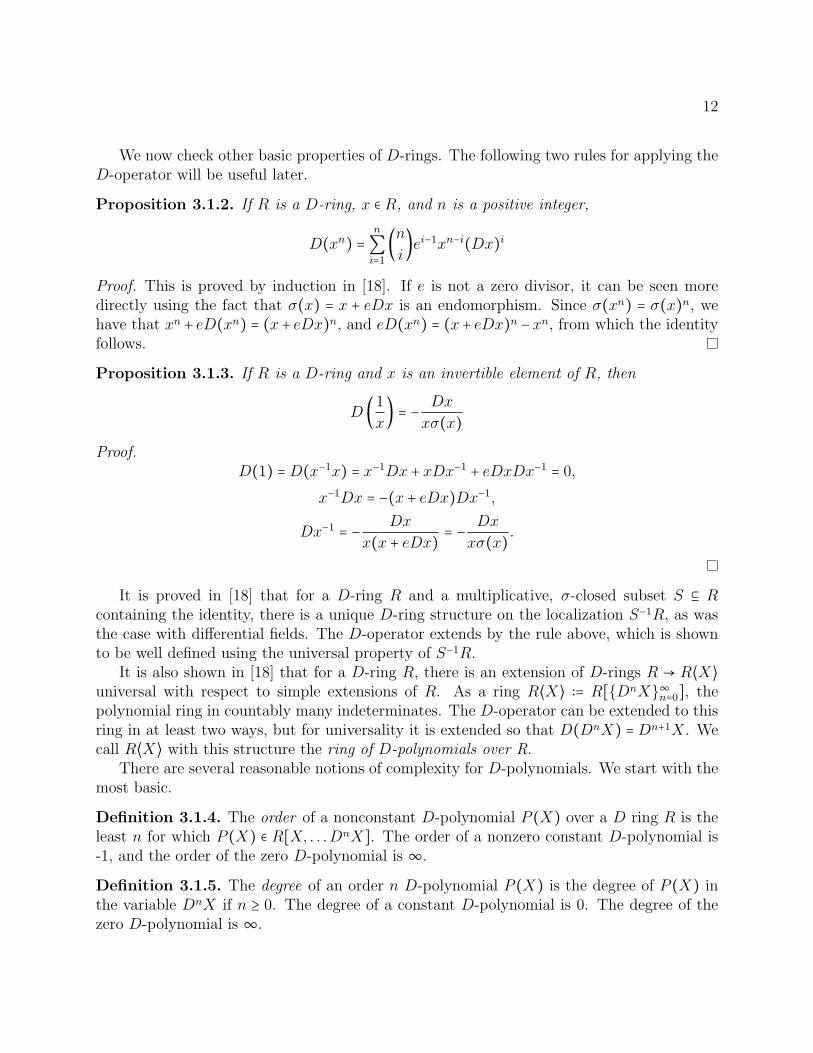
We now check other basic properties of D-rings. The following two rules for applying theD-operator will be useful later.

Proposition 3.1.2. If R is a D-ring, x ∈ R, and n is a positive integer,

D(xn) =

n

�i=1�n

i�e

i−1x

n−i(Dx)

i

Proof. This is proved by induction in [18]. If e is not a zero divisor, it can be seen moredirectly using the fact that σ(x) = x + eDx is an endomorphism. Since σ(xn) = σ(x)n, wehave that xn + eD(xn) = (x+ eDx)n, and eD(xn) = (x+ eDx)n − xn, from which the identityfollows.

Proposition 3.1.3. If R is a D-ring and x is an invertible element of R, then

D �1

x� = −

Dx

xσ(x)

Proof.

D(1) =D(x−1

x) = x−1

Dx + xDx−1+ eDxDx

−1= 0,

x−1

Dx = −(x + eDx)Dx−1

,

Dx−1= −

Dx

x(x + eDx)= −

Dx

xσ(x).

It is proved in [18] that for a D-ring R and a multiplicative, σ-closed subset S ⊆ R

containing the identity, there is a unique D-ring structure on the localization S−1R, as wasthe case with differential fields. The D-operator extends by the rule above, which is shownto be well defined using the universal property of S−1R.

It is also shown in [18] that for a D-ring R, there is an extension of D-rings R → R�X�

universal with respect to simple extensions of R. As a ring R�X� ∶= R[{DnX}∞n=0], thepolynomial ring in countably many indeterminates. The D-operator can be extended to thisring in at least two ways, but for universality it is extended so that D(DnX) =Dn+1X. Wecall R�X� with this structure the ring of D-polynomials over R.

There are several reasonable notions of complexity for D-polynomials. We start with themost basic.

Definition 3.1.4. The order of a nonconstant D-polynomial P (X) over a D ring R is theleast n for which P (X) ∈ R[X, . . .DnX]. The order of a nonzero constant D-polynomial is-1, and the order of the zero D-polynomial is ∞.

Definition 3.1.5. The degree of an order n D-polynomial P (X) is the degree of P (X) inthe variable DnX if n ≥ 0. The degree of a constant D-polynomial is 0. The degree of thezero D-polynomial is ∞.

13

A D-polynomial of order n and degree d has order-degree (n, d). Order-degrees areordered lexicographically, and a D-polynomial P is said to be simpler than a D-polynomialQ, denoted P � Q if the order-degree of P is less than the order-degree of Q in that ordering.

In the next example, we apply D to an order one D-polynomial over the constants, toprovide some insight into the structure of R�X�.

Example 3.1.6. Let R be a D-ring and P (X) = ∑ni=0 ciX

i be a polynomial over the constantsof R. Then

D(P (X)) =

n

�i=1

ei−1(DX)

i�

n

�m=i�m

i�cmX

m−i�

Proof.

D �

n

�i=1

ciXi� =

n

�i=1

ciD(Xi) =

n

�i=0

ci �

i

�k=0�i

k�e

k−1X

i−k(DX)

k� ,

then regroup around ek−1(DX)k.

As expected, applying the D-operator increases the order of P . However, unlike in adifferential field, the degree of D(P ) is the same as the degree of P , as the last term of D(P )

will be cnen−1(DX)n. When we move to valued D-fields, the “en−1” in this expression will

assure that such terms of high degree will also have high valuation.In Chapter 5, we will use a lemma from [18] that requires a more refined notion of

complexity for an inductive argument.

Definition 3.1.7. The total degree of a D polynomial P , denoted T.deg(P ), is (degX(i) P )∞i=0.For any P , T.deg(P ) ∈ N<ω ∶= {(nj)

∞j=0 ∶ nj ∈ N and nj = 0 for j � 0}. The set N<ω is

well ordered by (nj)∞j=0 < (mj)

∞j=0 if and only if there is some N such that nN < mN and for

all j > N , nj ≤ mj. With this ordering on the total degrees, we write P � Q if T.deg(P ) <T.deg(Q). This means that P � Q if there is some N for which degDN P < degDN Q and forall higher order terms, the degree of P never exceeds the degree of Q.

In addition to applying the D operator to D-polynomials, we will also want to be able totake their derivatives. If P is a D-polynomial of the form P (X) = F (X,DX, ...,DnX), define

∂∂X(i)P to be the D-polynomial ∂

∂XiF (X,DX, ...,DnX), the derivative of F with respect to

the variable DiX. We will need this primarily to make sense of a version of Hensel’s lemmafor valued D-fields; however in [18], it is used extensively in inductive arguments on T.deg,since for any i, ∂

∂X(i)P � P .

3.2 Valued Fields

We will look at De-rings in the context of valued fields. Recall the definition of a valuedfield.

14

Definition 3.2.1. A valued field is a pair (K,v) where K is a field and v is a map from K

onto Γ ∪ {∞}, where Γ is an ordered abelian group, called the value group and

1. v(x) =∞⇔ x = 0,

2. v(xy) = v(x) + v(y) (so v is a group homomorphism K× → Γ), and

3. v(x + y) ≥min{v(x), v(y)} (the “ultrametric inequality”).

From these axioms, we can conclude that v(x + y) > min{v(x), v(y)} then v(x) = v(y).Suppose x + y = z and v(z) > v(x) and v(z) > v(y). Then v(y) = v(z − x) ≥ v(x) andv(x) = v(z − y) ≥ v(y), which is only possible if v(x) = v(y).

For a valued field let K, we let RK denote the ring of integers of K, so RK ∶= {x ∈ K ∶

v(x) ≥ 0}. This ring has a unique maximal ideal mK ∶= {x ∈ K ∶ v(x) > 0}, and the quotientR�m is the residue field of K, denoted kK . The subscripts are dropped when doing so willnot cause confusion. The quotient map R → R�m is denoted π.

Definition 3.2.2. An extension L ⊇ K of valued fields is immediate if L and K have thesame value group and residue field.

Definition 3.2.3. An extension L ⊇K of valued fields is ramified if the value group of L isstrictly larger than the value group of K, i.e. ΓL � ΓK .

Definition 3.2.4. A valued field is said to be maximally complete if it has no proper im-mediate extensions.

Kaplansky showed in [10] that valued fields of residue field characterstic zero have uniquemaximal immediate extensions, and described the structure of such extensions. A key toolin his proof, and in much subsequent work in valued fields, was the existing notion of apseudo-convergent sequence.

Definition 3.2.5. A pseudo-convergent sequence is a limit ordinal indexed sequence {xα}α<κof elements of a valued field K such that (∀α < β < γ < κ) (v(xα − xβ) < v(xβ − xγ)).

If there is some c ∈ K such that (∀α < β < κ) (v(xα − c) < v(xβ − c)), then c is a pseudo-

limit of {xα}, and {xα} pseudo-converges to c.For any pseudo-convergent (p.c.) sequence {xα} in K, {v(xα−xα+1)} is a strictly increas-

ing sequence in ΓK . It is unbounded if and only if {xα} is a convergent sequence; otherwise,it isolates a cut in ΓK .

Define the the breadth of a p.c. sequence {xα} to be {ρ ∈ Γ ∪∞ ∶ (∀α)v(xα − xα+1) < ρ};so a p.c. sequence converges if and only if its breadth is {∞}. Let c be a pseudolimit of{xα}. Then any element b ∈K (or in any extension of K) satisfying v(b− c) ∈ breadth({xα})

is also a pseudolimit of {xα} (and conversely).If {xα} has no pseudo-limits in K, then it is a strict pseudo-convergent sequence.

15

An important attribute of some valued fields is satisfying a condition known as Hensel’sLemma, which can be stated in many equivalent forms. The one we will make the most useof is the following.

Hensel’s Lemma: Let K be a valued field and R its valuation ring. Given any P (x) ∈ R[x]

and a ∈ R satisfying v(P (a)) > 0 and v(P ′(a)) = 0, there is a b ∈ R with P (b) = 0 andv(a − b) > 0.

Not all valued fields satisfy Hensel’s lemma, but it is a powerful tool in those that do.Valued fields in which Hensel’s lemma holds are said to be henselian. All maximally completevalued fields are henselian, but the converse is false. Every valued field K has a henselisation

Kh, an immediate extension universal for extensions of K satisfying Hensel’s lemma.

Valued fields have long been objects of interest to model theorists, dating from at leastthe 1950’s. A good survey of the interactions of between model theory and the study ofvalued fields is given in the introduction to [4]. In particular, because of the ordering on thevalue group, no theory of valued fields can be stable. However, the theory of algebraicallyclosed valued fields, called ACVF, is an especially tractable example of an unstable theory,because it is largely controlled by a stable part. This is explored very precisely in [5], wherea notion called “metastability” is introduced. It is also shown in [5] that algebraically closedvalued fields have elimination of imaginaries in a reasonable extension of the standard valuedfield language, a result which can also be taken as a complete description of the un-eliminableimaginaries in the natural language.

3.3 �VDF: Axioms and Consequences

As noted above, D-rings generalize rings with both difference and differential operators.Valued D-fields allow us to consider these two cases in the same structure.

Definition 3.3.1. A valued D-field is a valued field K considered as a De-ring, with v(e) ≥ 0and v(Dx) ≥ v(x).

Since K is a field, e must be 0 or invertible. For the case of interest in this thesis, wetake e ≠ 0 and v(e) > 0. The D-operator on K is then interdefinable with an endomorphismof K, while the structure induced on k by D is that of a differential field.

In [18], the model theory of a particular class of these valued D-fields, there called (k,G)-D-henselian fields, is developed. We now present the axioms for these fields, as they appearin that paper.

The sorts are (K,k,Γ) where K is a valued field, k its residue field, and Γ its value group.The fields K and k, both of characteristic zero, are considered in the language of De rings.In the model completion, k will be linearly differentially closed, in the following sense.

16

Definition 3.3.2. A differential field k is linearly differentially closed if any non-zero lineardifferential operator L ∈ k[D] is surjective as a map L ∶ k → k.

The group Γ is an ordered abelian group with divisibility predicates; k and Γ may alsohave additional structure. A symbol ∞ is added to the language in a natural way, and thereare maps v ∶ K → Γ ∪∞ for the valuation and π ∶ K → k ∪∞ for the residue map. The ringof integers in K is definable, and denoted OK ∶= {a ∈ K ∶ v(a) ≥ 0}. The constants of K arealso definable and for now denoted KD ∶= {a ∈K ∶D(a) = 0}.

Definition 3.3.3. Let k be a linearly differentially closed field, also closed under nth roots.Let G be an ordered abelian group, and suppose that that Th(k) and Th(G) eliminatequantifiers. A (k,G)-D-valued field is a multisorted structure with sorts (K,k,Γ) satisfyingthe following axioms:

1. K and k are De fields of characteristic zero and k � Th∀(k).2. K is a valued field, whose value group is a subgroup of Γ via the valuation v and whose

residue field is a subfield of k via the residue map π, and v(e) > 0.

3. ∀x ∈K,v(Dx) ≥ v(x) and π(Dx) =Dπ(x) .

4. Γ � Th∀(G).

Definition 3.3.4. A (k,G)-D-henselian field is a structure satisfying the four axioms above,as well as:

5. (∀x ∈K) [([∃y ∈K]yn = x)↔ n�v(x)] .

6. Γ = v((KD)×) (“K has enough constants”).

7. k = π(OK) (“π is onto”).

8. (D-Hensel’s Lemma): If P ∈ OK�X� is a D-polynomial, a ∈ O, and v(P (a)) > 0 =v(

∂∂X(i)P (a)) for some i, then there is b ∈K with P (b) = 0 and v(a − b) ≥ v(P (a)).

9. Γ ≡G

10. k ≡ k

The theory of (k,G)-D-Henselian fields theory is model complete, and eliminates quan-tifiers in the field sort, up to the theories of the residue field and value group.

17

Example 3.3.5. As described in [18], for a fixed G and k the generalized power series fieldsk((εG)) provide canonical models for the theory of (k,G)-D-henselian fields. These fieldsare defined as a set by:

k((εG)) ∶= {f ∶G→ k ∶ supp(f) ∶= {x ∈ G ∶ f(x) ≠ 0} is well-ordered in G}.

Elements in k((εG)) can be considered as formal power series

f ↔ �γ∈G

f(γ)εγ

with addition and multiplication defined in the expected way.For f ∈ k((εG)), v(f) =min{supp(f)}. To determine D(f), let ∂ be the derivation on k

and let e be any element with v(e) > 0. On k, define

σ(x) =

∞�n=0

∂nx

n!e

n

and extend σ to the rest of k((εG)) by

σ(f) = �γ∈G

σ(f(γ))εγ.

Then D(f) can be recovered by the identity Df = e−1(σ(f) − f). With this structure,k((εG)) is a maximally complete as a valued field, and thus henselian.

We will often work in these fields and use model completeness to draw more generalconclusions.

Notation 3.3.6. Of special interest in this thesis are (k,G)-D-henselian fields for k dif-ferentially closed. We call the theory of (k,G)-D-Henselian fields for k differentially closed�VDF. Any (k,G)-D-field K can be embedded into a model M of �VDF; take M to be a(k′,G)-D-Henselian field where k′ is a differential closure of k. This will be discussed inmore detail in Chapter 5.

From this point on, we will refer to a D-operator on a valued field K as D, and theD-operator induced on the residue field as ∂, as a reminder that the residue operator is infact a derivation (so the second half of Axiom 3 would now read “π(Dx) = ∂π(x)”). Tofurther emphasize the connection with differential fields, we will from now on refer to theconstants of K as CK and the constants of k as Ck. A D-henselian field is any valued D-fieldtin which the D-Hensel’s Lemma holds.

18

3.4 Algebra in Valued D-Fields

In this section, we explore basic algebra in the valued D-field setting, and establish somefacts that will be useful in what follows.

First, note that the requirement that v(Dx) ≥ v(x) implies that the endomorphismdefined by σ(x) = x + eDx is valuation preserving. In fact, we can say more. In [4] andelsewhere, valued fields are considered with their leading term or “RV” structure. For x ∈K×,rv(x) is the image of x in the quotient K×�(1 +m). Thus, for x, y ∈K, rv(x) = rv(y) if andonly if v(x − y) >min{v(x), v(y)}; equivalently, if v(x − y) > v(x) or v(x − y) > v(y).

For any δ ∈ Γ with δ > 0, we can also consider the ideal mδ ∶= {x ∈ R ∶ v(x) > δ}, and setrvδ(x) to be the image of x in K×�(1 +mδ), so rv0(x) = rv(x), and if α,β ∈ Γ with α < β,then for any x, y ∈K, rvβ(x) = rvβ(y) implies rvα(x) = rvα(y). The image of the map rvδ isthe uneliminable imaginary sort RVδ.

Proposition 3.4.1. If K is a valued D-field with v(e) > 0, and σ is the endomorphism

defined by σ(x) = x + eDx, then rv(xσ) = rv(x).

Proof. The endomorphism σ takes x and adds to it something of strictly higher valuation,thereby preserving the leading term. By the definition of valued D-field, v(Dx) ≥ v(x), andby assumption v(e) > 0, so v(eDx) = v(Dx) + v(e) > v(x). Then since

xσ− x = eDx

we have v(xσ − x) > v(x). By the above, this is equivalent to rv(xσ) = rv(x).

Next, a few remarks about henselizations.As we will be dealing mostly with linear equations, it is worth noting that if P (X) =

∑ni=0 ri D

i(X) is a linear D-equation with min{v(ri)} = 0, then P satisfies the hypotheses of

the D-Hensel’s Lemma at any approximate root, since ∂∂X(j)P (a) = rj regardless of the choice

of a. Therefore, when working with linear equations in D-henselian fields, we will apply DHLwithout rechecking this condition.

One major complication in going from the study of differential fields to the study ofdifference fields is that, in a difference field, elements algebraic over the constants may notbe constant themselves. Instead, they might be elements of finite orbit under the differenceoperator. Difference fields that have algebraically closed fields of constants are in many waysmuch simpler than those that do not, and many theorems of differential algebra apply onlyto the restricted case of such fields.

In �VDF, the restriction that the algebraic closure of the constants contains no nonconstantelements is a consequence of the axioms.

Proposition 3.4.2. If K is a D-henselian field with enough constants, then CK is relatively

algebraically closed in K; if a ∈K is algebraic over CK, then Da = 0.

Proof. We must first establish the following weaker claim.

19

Claim. If K is a valued D-field with enough constants, and a ∈K is algebraic over CK and

a ≠ 0, then v(Da) > v(a).

Proof. Our definition of valued D-field requires that for all x ∈ K, v(Dx) ≥ v(x). We showthat for a CK-algebraic, the inequality must be strict.

Since there are constants at every valuation, we may scale by a constant to assume thatv(a) = 0. Let

P ∶=

n

�i=0

cixi

be a minimal polynomial for a over CK . We may again scale to assume that P is minimallyintegral; ie min{v(ci)} = 0. Then π(P ) is a nonzero polynomial over the constants of theresidue field, and π(a) is a solution to π(P )(x) = 0. Since the residue field is a differentialfield, anything algebraic over the constants is itself a constant, and ∂(π(a)) = π(Da) = 0, sov(Da) > 0 = v(a).

Now, suppose that there were some a ∈ K, algebraic over CK , with Da ≠ 0. Again,we may assume without loss that v(a) = 0 and that a has a minimally integral minimalpolynomial P over CK .

From the above, we know that v(Da) > 0. Let v(Da) = α. If Q(x) ∶= Dx, then v(Q(a)) =

v(Da) > 0, and ∂∂X(1)Q(a) = 1, so v(

∂∂X(1)Q(a)) = 0, and DHL applies to Q at a. From this,

we can find a b ∈K such that D b = 0 and v(a− b) ≥ v(Da) = α. Now consider m ∶= a− b. Theelement m is algebraic over the constants, as it satisfies P (x+ b) = 0, v(m) = v(a− b), whichby DHL is at least α, and v(Dm) = v(D(a − b)) = v(Da −D b) = v(Da) = α, contradictingthe previous claim.

Corollary 3.4.3. If K is a valued D-field, then CK is relatively algebraically closed in K;

if a ∈K is algebraic over CK, then Da = 0.

Proof. Any valued D-field K can be extended to a D-henselian field L with enough constants.

As we plan to consider linear D-equations, it will be useful to recall the definition of theWronskian and to define its D-analogue.

Definition 3.4.4. If y1, ..., ys are elements of a differential ring R, then their Wronskian, de-noted w(y1, ..., ys), is the determinant of the s×s matrix whose ith column is (yi,∂yi, . . .∂

s−1yi)�

This notion may be extended to any D-ring, where D may not be a derivation.

Definition 3.4.5. If y1, ..., ys are elements of a D-ring T , then their D-Wronskian, denotedwD(y1, ..., ys), is the determinant of the s×s matrix whose ith column is (yi,D yi, . . .D

s−1yi)�

20

When it is clear from the context that we are working in the D-ring setting, this will bereferred to simply as the Wronskian and denoted w(y1 . . . ys) as in the differential case.

In a differential field F , elements y1, . . . , yn ∈ F are linearly independent over the constantsof F if and only if w(y1, . . . , ys) = 0. This is also true in D-fields. The standard proofs fordifferential fields work with slight modifications; the key is the following simple observation.

Proposition 3.4.6. Let K be a field and σ an automorphism of K. Let y1, . . . , yn ∈ K.

Then y1, . . . , yn are linearly dependent over the σ-constants CσK of K if and only if yσ

1 , . . . , yσn

are.

Proof. Suppose ∑ni=1 ciy

σi = 0 with ci ∈ C

σK , not all zero. Then

σ−1�

n

�i=1

ciyσi � =

n

�i=1

σ−1(ciy

σi ) =

n

�i=1

ciyi = σ−1(0) = 0.

From here we follow [11], using the twisted Leibniz rule in the form D(ab) = aDb+ bσDa.The above lemma will allow us to work with the twisting.

Lemma 3.4.7. Let K be a valued D-field with field of constants CK. Then y1, . . . , yn are

linearly dependent over CK if and only if w(y1 . . . yn) = 0.

Proof. In the first direction, if (y1, . . . yn) are linearly dependent over CK , there are c1, . . . , cn ∈

CK such that ∑ni=1 ciyi = 0. Applying Dj to this equation, we see that ∑n

i=1 ci Djyi = 0 for any

j, and so the ci’s are a nontrivial solution to the system of linear equations

n

�i=1(Dj

yi)xi = 0 for 0 ≤ j ≤ n − 1.

The determinant of the matrix of coefficients of this system is w(y1, . . . , yn), which musttherefore be zero.

On the other hand, if w(y1, . . . , yn) = 0, then there are c1 . . . cn ∈ K such that for 0 ≤ j ≤

n − 1:n

�i=1(D

jyi)ci = 0

To show that all the ci can be taken to be in CK , arrange the indices so that c1 ≠ 0, thendivide through by c1 to let c1 = 1. Then apply D to obtain

n

�i=1(Dj+1

yi)ci +

n

�i=1

σ(Djyi)D(ci) = 0

21

For 0 ≤ j ≤ n − 2, the first sum is zero by the preceding equation. Since c1 = 1, D(c1) = 0,and the first term in the second sum is also zero. So for 0 ≤ j ≤ n − 2, D(c2), . . . ,D(cn) is asolution to the system of linear equations

n

�i=2

σ(Djyi)xi =

n

�i=2(Dj

σ(yi))xi = 0

The determinant of the matrix of coefficients for this equation is w(yσ2 , . . . , yσ

n). If w(yσ2 , . . . , yσ

n) ≠

0, then the solution D(c2), . . . ,D(cn) trivial, so yσ2 , . . . yσ

n are linearly dependent over CK , andso are y2 . . . yn. If w(yσ

2 , . . . , yσn) = 0, proceed by induction until a linear dependence relation

between yσm

i , . . . , yσm

n over CK is found for some i and m. Applying σ−m then gives a relationbetween yi, . . . , ym without changing the coefficients.

22

Chapter 4

Solutions to Linear D-Equations

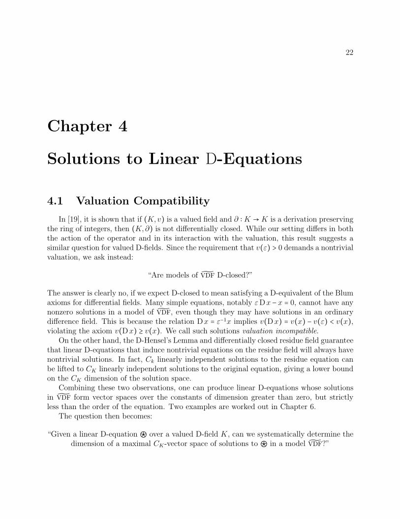
4.1 Valuation Compatibility

In [19], it is shown that if (K,v) is a valued field and ∂ ∶K →K is a derivation preservingthe ring of integers, then (K,∂) is not differentially closed. While our setting differs in boththe action of the operator and in its interaction with the valuation, this result suggests asimilar question for valued D-fields. Since the requirement that v(ε) > 0 demands a nontrivialvaluation, we ask instead:

“Are models of �VDF D-closed?”

The answer is clearly no, if we expect D-closed to mean satisfying a D-equivalent of the Blumaxioms for differential fields. Many simple equations, notably εDx − x = 0, cannot have anynonzero solutions in a model of �VDF, even though they may have solutions in an ordinarydifference field. This is because the relation Dx = ε−1x implies v(Dx) = v(x) − v(ε) < v(x),violating the axiom v(Dx) ≥ v(x). We call such solutions valuation incompatible.

On the other hand, the D-Hensel’s Lemma and differentially closed residue field guaranteethat linear D-equations that induce nontrivial equations on the residue field will always havenontrivial solutions. In fact, Ck linearly independent solutions to the residue equation canbe lifted to CK linearly independent solutions to the original equation, giving a lower boundon the CK dimension of the solution space.

Combining these two observations, one can produce linear D-equations whose solutionsin �VDF form vector spaces over the constants of dimension greater than zero, but strictlyless than the order of the equation. Two examples are worked out in Chapter 6.

The question then becomes:

“Given a linear D-equation � over a valued D-field K, can we systematically determine thedimension of a maximal CK-vector space of solutions to � in a model �VDF?”

23

The answer to this question is yes. In fact, the example of εDx−x = 0, which specializesto x = 0 in the residue field, demonstrates the only hurdle to adjoining solutions to a linear D-equation in �VDF. The CK dimension of the solution space of a linear D-equation is completelydetermined by the structure it induces on the residue field.

To arrive at this result, we first need a few definitions.

Definition 4.1.1. A D-polynomial P (X) over a valued D-field K is said to be minimally

integral the minimum of the valuations of its coefficients is zero. Equivalently, P is over R

and π(P ) ≠ 0.

Since K is a field, any D-polynomial over K is equivalent to one in minimally integralform. Suppose v(b) =min{v(aS) ∶ aS is a coefficient of P}; then b−1P is a minimally integralpolynomial with the same zero set as P .

For a given polynomial, this minimally integral form is not unique, but the valuationsof the coefficients are. Furthermore, if P is of order n, we can take the coefficients of P tobe indexed by Nn in the natural way and ordered lexicographically, and can always assumethat P has been scaled by the coefficient whose index is greatest among those of minimalvaluation. This will ensure that the corresponding polynomial in the residue field is monic.

Definition 4.1.2. The residual order of a minimally integral D-polynomial P is the greatestn such that Dn appears in some term of P whose coefficient has valuation zero. Equivalently,π(P ) has order n as a ∂-polynomial on k.

A linear D-operator L ∶= ∑ai D(i) is minimally integral if min{v(ai)} = 0. In that case,

its residual order is max{i ∶ v(ai) = 0}, the order of the operator induced on the residue field.

For the remainder of this section, K is a valued D-field with enough constants, satisfyingD-Hensel’s lemma, with value group Γ, residue field k, and ring of integers R. We let L bea minimally integral linear D-operator over K and l ∶= π(L) the ∂-operator induced on k byL.

We will show that the solutions to L in K form a vector space over CK of dimension equalto the dimension of the Ck vector space of solutions to l in k. If k is differentially closed, orat least closed with respect to linear differential equations, this dimension will be equal tothe residual order of L. The first step is to establish a connection between the solutions toL in K and the solutions to l in the k.

Lemma 4.1.3. Let K, k, L, and l be as above, and suppose that a1, . . . , an are solutions

to l in k, linearly independent over Ck. Then there are A1, . . . ,An ∈ R, such that for all i,

π(Ai) = ai, L(Ai) = 0, and A1, . . . ,An are linearly independent over CK.

Proof. Since π is onto, there are elements B1, . . . ,Bn ∈ R with π(Bi) = ai for all i. TheseBi are approximate solutions to the linear equation L = 0, so DHL applies to L at each Bi,giving A1, . . . ,An ∈ R, with π(Ai) = ai and L(Ai) = 0.

24

Suppose that ∑ni=1 ciAi = 0 with ci ∈ CK not all zero. By scaling and rearranging terms

we may assume that for all i, ci ∈ R, and that v(c1) = 0. Then ∑ni=1 π(ci)ai = 0, each π(ci) is

a constant, and π(c1) ≠ 0.

We will also need the following definition.

Definition 4.1.4. For X ⊆K a definable set and a ∈K the proximity of a to X is ρ(a,X) ∶=

sup{v(a − x) ∶ x ∈X}.

Since X is definable, so is {v(a−x) ∶ x ∈X}. If the value group is divisible, it is o-minimal,and every definable set will have a supremum, so ρ(a,X) will be a well defined element ofthe value group. If the value group is not o-minimal, the type of ρ(a,X) may not be realizedin Γ. The proximity ρ(a,X) is then the cut described by this type.

When X is the zero set of some D-polynomial P (x), another reasonable measure ofproximity would be the distance from P (a) to zero, which will always exist. The nextlemma shows that, in many important cases, the two measures will be the same.

Lemma 4.1.5. Suppose that P (x) ∈ R[x]D is a D-polynomial over R, a ∈ R, and DHL

applies to P at a. Let X ∶= {b ∈ K ∶ P (b) = 0}. Then ρ(a,X) = v(P (a)), and there is some

b ∈X for which this proximity is attained.

Proof. For any c ∈ R, P (a) ≡ P (c) mod v(a−c). If c ∈X, P (c) = 0 and P (a) ≡ 0 mod v(a−c),so v(a − c) cannot exceed v(P (a)). Therefore ρ(a,X) is bounded above by v(P (a)). ByDHL, there is some b ∈ X with v(a − b) ≥ P (a), so ρ(a,X) is at least v(P (a)), and the twoare equal. For the b provided by DHL, v(a − b) = v(P (a)) = ρ(a,X).

With this in hand, we move onto the main result.

Theorem 4.1.6. Let L be a minimally integral linear D-operator over a D-henselian field

K with enough constants, and suppose that the solutions to l ∶= π(L) form an n-dimensional

Ck vector space in the residue field k. Then the solutions to L in K have dimension n as a

CK-vector space.

Proof. Suppose that L ∶= ∑mi=0 ai D

(i) has order m. It is clear that the solutions to L form avector space V over CK of dimension at most m.

Because the residue field k is a differential field, the solutions to l ∶= π(L) are a vectorspace over Ck, the constants of the residue field, which we assume to have dimension n ≤m.By Lemma 4.1.3 any basis of this vector space can be lifted to n linearly independent solutionsto L in K, so the dimension of V is at least n.

It remains to be shown that the dimension of V is at most n. To do this, we will start withthe n-dimensional CK vector space established above, and demonstrate that any solution a

to L = 0 in K is in this vector space.Suppose we have f1, . . . , fn ∈ R, linearly independent over CK with Lfi = 0, v(fi) = 0, and

π(f1), . . . ,π(fn) linearly independent over Ck.

25

Let U be the CK vector space generated by {f1, . . . , fn}, and let Q(x) ∶= w(f1, . . . , fn, x).By Lemma 3.4.7, the set of solutions to Q(x) = 0 is exactly U .

Let T be the Ck vector space generated by {π(f1), . . . ,π(fn)}. By our assumptions,we know that T can also be viewed as the space of solutions to l in the residue field, i.e.T ∶= {x ∈ k ∶ ∑

ni=0 π(ai)∂

ix = 0}.

Lemma 4.1.7. If Q(x) ∶= w(f1, . . . , fn, x), then∂Q

∂Xn= (−1)nw(f1, . . . , fn). In particular, its

valuation is always zero.

Proof. By expanding w(f1, . . . , fn, x) along the last column, we obtain

Q(x) =

n

�i=0(−1)i Di

(x) ⋅ �Mi�

where Mi is the n × n matrix whose jth column is (fj . . .Di−1fj,D

i+1fj, . . .D

n+1fj)

T. Thecoefficient of Dn

(x) in this expansion is (−1)nw(f1, . . . , fn), so ∂Q∂Xn= (−1)nw(f1, . . . , fn).

Since we have taken {π(f1), . . . ,π(fn)} to be linearly independent over the constants ofthe residue field, π(w(f1 . . . fn)) = w(π(f1), . . . ,π(fn)) ≠ 0, so v(w(f1, . . . , fn)) = 0.

Lemma 4.1.8. If La = 0, then there is some b ∈ U with v(a − b) = ρ(a,U).

Proof. Since Q(x) = 0 exactly when x ∈ U , we must find a b ∈ K with Q(b) = 0 andv(a − b) = ρ(a,U).

Since La = 0, π(a) is a solution to l = 0, and can be expressed as a Ck-linear combinationof {π(f1), . . . ,π(fn)}. Therefore, π(Q(a)) = w(π(a),π(f1), . . . ,π(fn)) = 0, and Q(a) hasvaluation greater than 0.

By Lemma 4.1.7 ∂Q∂Xn(a) = w(f1, . . . , fn), which has valuation zero. Therefore, DHL

applies to Q at a, and by Lemma 4.1.5 such a b must exist.

Lemma 4.1.9. For any � ∈ Γ, there is an injective linear map {x ∈ K ∶ Lx = 0 & v(x) ≥

�}�{x ∈K ∶ Lx = 0 & v(x) > �}→ T

Proof. Pick c ∈ CK with v(c) = −�. For y ∈ {x ∈K ∶ Lx = 0 & v(x) ≥ �}, let F ∶ y � cy. ThenG ∶= π ○F is a linear map from {x ∈K ∶ Lx = 0 & v(x) ≥ �} to T . If y1 and y2 have the sameimage under G, then y1 − y2 ∈ {x ∈ K ∶ Lx = 0 & v(x) > �}, so the map induced by G from{x ∈K ∶ Lx = 0 & v(x) ≥ �}�{x ∈K ∶ Lx = 0 & v(x) > �} to T is injective and linear.

Lemma 4.1.10. For any � ∈ Γ and y ∈ R with Ly = 0, there is an injective affine map {x ∈

K ∶ Lx = 0 & v(x − y) ≥ �}�E� → T where E� is the equivalence relation xE�y ∶= v(x − y) > �.

Proof. If Lx = 0, then L(x − y) = 0. Now apply Lemma 4.1.9.

26

For a fixed y ∈ R with Ly = 0, set Vy,� ∶= {x ∈ K ∶ Lx = 0 & v(x − y) ≥ �}�E� as above.Then Vy,� is a vector space over CK�E0 ≅ Ck. Since the map in Lemma 4.1.10 is injective, itmust have dimension less than or equal to n.

Similarly, let Uy,� be {x ∈ K ∶ Qx = 0 & v(x − y) ≥ �}�E�. It is also a vector space overCK�E0 ≅ Ck, of dimension exactly n. By a translating and scaling as above, we can constructfor any y ∈ U and � ∈ Γ an isomorphism Uy,� ≅ T .

Lemma 4.1.11. If La = 0, then a ∈ U

Proof. Suppose La = 0, but a ∉ U . Let α ∶= ρ(a,U), and take b ∈ U with v(a − b) = α.Let a be the equivalence class of a in Vb,α, so a consists of elements of x ∈ V with

v(x − a) > α and let z be its image under the above injection ι ∶ Vb,α � T , so z is an elementof k. If c is the constant used in Lemma 4.1.9, then z = π(c(a − b)).

Let b be the class of Ub,α that maps to z under the same translation and scaling, whichmust exist since the map from Ub,α to T is an isomorphism. Let r be a representative of b;since we used the same scaling as above, this means π(c(r − b)) = z.

Since U ⊆ V , r ∈ V . Because r ∈ V and v(r− b) ≥ α, r ∈ Vb,α. From the fact that r ∈ b andι(b) = z, it follows that r ∈ a.

So r ∈ U , and v(a − r) > α, a contradiction.

Equivalently, since π(c(a − b)) = z and π(c(r − b)) = z, v(c(a − b) − c(r − b)) > 0, sov(c(a − r)) = v(c) + v(a − r) > 0, and v(a − r) > −v(c) = α.

The translation and scaling in Lemmas 4.1.9 and 4.1.10 may also be seen directly in thefollowing calculation:

Let a, b and α be as above, and let d ∶= a − b, so Ld = La − Lb = 0 and v(d) = α. Find ac ∈ CK with v(c) = −α, which must exist because K has constants at every valuation, andlet g ∶= cd. Note that g ∈ U if and only if a ∈ U .

Since g is a solution to Lx = 0, by the same argument used above for a, DHL applies toQ at g, providing an h ∈ U with v(g − h) > 0. Let j = g − h and r = b + c−1h. Since b and h

are both in U , so is r. Then

v(a − r) = v(a − (b + c−1(h))

= v(a − (b + c−1(g + j))

= v(a − b − c−1(c(a − b) + j)

= v(a − b − (a − b) − (c−1

j))

= α + v(j)

> α

So either a ∈ U and therefore ρ(a,U) = ∞, or as above we have found r ∈ U withv(a − r) > ρ(a,U), a contradiction.

27

From this, it follows that V = U and dim(V ) = n.

Corollary 4.1.12. Let L be a minimally integral linear D-operator of residual order n over

K � �VDF. Then the solutions to L in K form an n-dimensional vector space over the

constants of K.

Proof. Since K ��VDF, it is a D-henselian field with enough constants, so the above theoremapplies. As k is differentially closed, the solutions to π(L) in k will have dimension n as aCk-vector space.

4.2 D-fundamental systems of solutions

Given a linear D-equation� over a valued D-field K, we will be interested in adjoining asmany solutions to� as possible without growing the constants. Therefore, sets of solutions to� that are maximal in this sense will play an important role. Keeping with the terminologyof difference and differential fields, we will call them D-fundamental systems of solutions.

Definition 4.2.1. A D-fundamental system of solutions of a linear D-equation � ofresidual order n over a valued D-field K is a n-tuple (f1 . . . fn) of elements in some extensionK ′ of K such that

● Each fi is a solution to �.

● The set {f1 . . . fn} is linearly independent over the constants of K ′.● The set {π(f1) . . .π(fn)} is linearly independent over the constants of π(K ′).● The constants of K�f1 . . . fn� are the constants of K.

In general, if L ⊇ K is an extension of valued D-fields and CL = CK , we call L a no new

constants extension of K.If K is a valued D-field whose constants CK form a maximally complete valued subfield

with residue field Ck algebraically closed, then any linear D-equation � over K will have afundamental system of solutions; a differential fundamental system will exist for the residueequation, and can be lifted by DHL. Lemma 5.1.1 assures that this can be done withoutadding to the value group. Since CK is assumed to be maximal, this implies that theextension will add no new constants.

If �f and �g are both fundamental systems of solutions to some linear D-equation � insome extension L of K, then �f = A�g where A is some matrix over CL; otherwise we couldconstruct a solution space CL dimension greater than n.

28

Chapter 5

Galois Theory

5.1 PVD-extensions

A vital element in the model theoretic approach to differential Galois theory is the ex-istence of unique prime models over arbitrary sets for DCF0, which provide a good notionof differential closure in which to work. However, the existence of unique prime models inDCF0 is consequence of the fact that the theory is totally transcendental. Because of theordering on the value group, �VDF is not even stable. It is not known, in general, whether�VDF such admits prime models. Therefore, it is not immediately clear that the field exten-sions generated by distinct fundamental systems of solutions to the same equation will beisomorphic. Fortunately, modulo a few reasonable assumptions on the constants of the basefield, we will see that they are.

The following lemma (7.12 in [18]) will be useful.

Lemma 5.1.1. Let K be a valued D-field. Given a type p ∈ S1,k(kK) and a D-polynomial

P ∈ OK�X� such that

● If x � p then π(P ) is of minimal total degree among nonzero Q(X) ∈ π(OK)�X� with

Q(x) = 0, and

● T.deg(P ) = T.deg(π(P )),

there is a unique (up to LK-isomorphism) D-field L =K�a� such that P (a) = 0 and π(a) � p.

The extension K ⊆ L is unramified.

The version of this lemma appearing in [18] does not include the condition that L isunramified in the statement of its conclusion; however, it is clear from the proof that thevalue group does not grow in the construction of K�a�.

29

Furthermore, the requirement that T.deg(P ) = T.deg(π(P )) is slightly stronger than isnecessary. In fact, what is needed in the proof is that order-degree of P is equal to the order-degree of π(P ) and that the highest degree term of any order occurring in P has nonzeroresidue. We will use this fact in the last example in Chapter 6.

The next necessary ingredient is a slight modification of Theorem 5.8 in [2]. There, Azginand van den Dries prove uniqueness for certain valued difference field extensions. Becausethe difference operators on their valued fields must induce nontrivial automorphisms theresidue fields, the result does not immediately apply to our valued D-field case, where theresidue field automorphism is the identity. However, by judiciously replacing σ with δ inmost of their proof, the following can be recovered.

Theorem 5.1.2. Let K be a valued D-field of equicharacteristic zero, whose residue field is

linearly differentially closed. All maximal immediate extensions of K are K-isomorphic.

Together, these two pieces allow us to prove the following extension of Theorem 5.1.2.

Theorem 5.1.3. Let K be a valued D-field with residue field k. Let k′ be the differential

closure of k. Then there is a maximal unramified extension K ′ ⊇ K with residue field k′,unique up to isomorphism over K.

Proof. To see that such a field must exist, note that for any valued D-field K and anyextension k′ of k, we can construct an unramified valued D-field extension L of K withresidue field k′ by repeatedly applying Lemma 5.1.1.

Now let K ′ be a maximal immediate extension of L. Such a K ′ must exist as the class ofimmediate extensions of L up to isomorphism is a set. This K ′ is an unramified extensionof K having k as its residue field.

If k′ is linearly differentially closed, such a K ′ is unique up to isomorphism over K.Given two candidate fields, we will show that they are isomorphic by first finding isomorphicintermediate subfields, then applying Theorem 5.1.2.

Lemma 5.1.4. Let K be a valued D-field with residue field k, and suppose k′ ⊇ k is linearly

differentially closed. If K1 and K2 are two maximal unramified valued D-field extensions

of K each with residue field k′, then there are subextensions L1 ⊆ K1 and L2 ⊆ K2 with

π(L1) = π(L2) = k′ and L1 ≅K L2.

Proof. By a back and forth argument, it suffices to show that for each a ∈ k′, there is ana1 ∈K1 and an a2 ∈K2 such that π(a1) = π(a2) = a and K�a1� ≅K K�a2�.

Given a ∈ k′, find a minimal D-polynomial Q for a over k, and a lifting P of Q to OK

such that the hypotheses of Lemma 5.1.1 apply. Since π(K1) = π(K2) = k′, there are bi ∈Ki

such that π(bi) = a. By the minimality of Q, there is some derivative of Q that does notvanish at a, so DHL applies to P at bi. Since K1 and K2 are maximal and k′ is linearlydifferentially closed, DHL holds in K1 and K2, giving ai ∈ Ki with π(ai) = a and P (ai) = 0.Then K�a1� ≅K K�a2� by Lemma 5.1.1.

30

Corollary 5.1.5. With notation as in Lemma 5.1.4, K1 and K2 are isomorphic over K.

Proof. Identifying L1 and L2 by the isomorphism in Lemma 5.1.4, K1 and K2 are bothmaximal immediate extensions of a valued field L whose residue field is linearly differentiallyclosed. The result then follows, as promised, by Theorem 5.1.2.

Given a linear D-equation � over a valued D-field K, and a fundamental system ofsolutions �f of � in some extension of K, K� �f� will be our analogue of a Picard-Vessiotextension for the equation �. With some restrictions on the constants of K ond k, thisextension is independent of the choice of �f , up to isomorphism over K.

Theorem 5.1.6. Let K be a valued D-field with CK maximal and π(CK) algebraically closed.

Let � be a linear D-equation over K and let �f and �g be D-fundamental systems of solutions

to �. Then Kf ∶=K� �f� and Kg ∶=K��g� are isomorphic over K.

Proof. As above, let k be the residue field of K, and let k′ be the differential closure of k.Since Ck is algebraically closed, Ck′ = Ck and the residue fields of Kf and of Kg embed intok′ over k.

By Theorem 5.1.3, we may find maximal unramified extensions K1 of Kf and K2 of Kg,both with residue field k′. Because Kf and Kg are unramified extensions of K, K1 and K2

are also maximal unramified extensions of K with a common differentially closed residuefield. By the theorem, they are therefore isomorphic over K. Via this isomorphism Kf andKg embed over K into a common maximally complete field M with residue field k′ and valuegroup ΓK .

Since �f and �g are fundamental systems of solutions for �, we have �f = A�g for somematrix of constants in M . By maximality of CK , CK = CM and we conclude that the imagesof Kf and of Kg in M are equal.

Note that the requirement that CK be maximal cannot be dropped, as shown in Example6.1.1.

5.2 Liaison Groups

We have shown that, given a linear D-equation � over a valued D-field K, we canassociate to � a unique valued D-field extension L generated by a D-fundamental system ofsolutions to �. We would now like to consider the automorphisms of this extension.

Let Q be the definable set of solutions to � and let C be the set of solutions to theequation Dx = 0. Then in any model M of �VDF, the set Q(M) of points of Q in M isa vector space over C(M), the constants of M. A basis of this vector space is given bya D-fundamental system �f of solutions to �, so the points of Q(M) are all definable over

31

{C(M) ∪ �f}. This remains true in any extension N ⊇ M; Q(N ) will be definable over{C(N ) ∪ �f} for the same �f . The definable set Q of solutions to � is therefore internal tothe definable set C of constants.

The group MGal(Q�C) of model theoretic automorphisms of Q over C can thus beidentified with a type definable group G, and in any U there is a Galois correspondencebetween type definable subgroups of G and definably closed subsets S of U eq with dcleq(C) ⊆S ⊆ dcleq(Q).

Elements of the automorphism group are determined by their action on the internalizingset �f . Since the image of �f under any automorphism will be another fundamental system ofsolutions to �, and any two fundamental systems of solutions differ by a constant matrix,there is a map from the model theoretic automorphism group into the GL(Q), the group oflinear transformations of the C vector space Q, which can be identified with GLn(C), usingthe basis �f .

As the theory �VDF has quantifier elimination, the structure preserved by this group isexactly that which can be described using quantifier free formulas. However, the presenceof the valuation map means that these quantifier free formulas will describe more thanthe algebraic structure. This means that the model theoretic automorphism group willbe a proper subgroup of the group preserving just the algebraic structure. Furthermore,subgroups of G can be defined using the valuation, leading to points on the group side ofthe Galois correspondence that do not occur as subgroups in the standard difference Galoiscorrespondence and therefore can not correspond to subfields.

This is related to the failure of �VDF to eliminate imaginaries. In DCF0, a consequence ofelimination of imaginaries is that in everyM � DFC0, every definably closed subset ofMeq

is actually a substructure ofM, so the “field” side elements of the Galois correspondence areactually fields. In �VDF, the “field” side elements of the correspondence will include at leastthe imaginaries of [5] coming from the valued field language, and possibly more, as shownin Example 6.2.1.

Finally, in a consequence of the ω-stability of DCF0 is that every type definable groupin that theory is actually definable. This also fails in �VDF; a simple example of an equationwith a model theoretic automorphism group that is type definable but not definable is givenin Example 6.3.1.

32

Chapter 6

Examples

In this chapter, we look at several linear D-equations equations and their solution spacesin models of �VDF. These examples are chosen to illustrate issues of definabilty and dimension,and to demonstrate the necessity of the maximality assumption on the constants in Chapter5. For most of these equations, we compute the model theoretic automorphism group of thesolutions space over some base field, usually the constants. We then compare these groupswith the traditional difference Galois groups associated to the same equations, and to thedifferential Galois groups of the equation induced on the residue field. In the difference fieldcase, we rely heavily on the algorithm from [6] outlined in the preliminaries.

To understand the internal structure of models of �VDF, we will need to consider valuationideals. These will allow us to look at approximations to solutions, and to iteratively constructsuch approximations. For α ∈ Γ, these ideals are m>α =∶ {x ∈ R ∶ v(x) > α} and m≥α =∶ {x ∈R ∶ v(x) ≥ α}. If a and b in R are such that v(a − b) > α or v(a − b) ≥ α, we will sometimeswrite a ≡>α b, or a ≡≥α b.

6.1 Maximality of Constants

The first example demonstrates the necessity of the requirement that the constants bemaximal in Theorem 5.1.6, by showing that uniqueness may fail if the constants are assumedonly to be algebraically closed.

Example 6.1.1. Let K be a valued D-field with enough constants, such that CK is alge-braically closed but not maximal. Assume that there is some a ∈ K with π(a) ≠ 0 suchthat the equation Dx = ax has no nonzero solutions in K, but ∂x = π(a)x has a full set ofsolutions in k, the residue field of K.

Let K ′ be a maximal immediate extension of K. Then CK′ is also maximal. Takec ∈ CK′ � CK with π(c) = 1. Such a c must exist because if d is any constant in CK′ � CK

with v(d) ≥ 0, then for any b ∈ CK with 0 < v(b) <∞, we can take c ∶= 1 + bd.

33

Let U ��VDF and take f ∈ U such that Kf ∶=K�f� ⊆ U is a no new constants extension ofK. Let g = cf and Kg ∶= K�g� ⊆ U . Then Kg and Kf are not isomorphic as valued D-fieldsover K. To see this it suffices to show that tp(g�K) is not realized in Kf .

Since the residue equation ∂x = π(a)x has a full set of solutions in k, we can build apseudoconvergent sequence {xα} approximating g in K, and therefore also in Kf . Then{f−1xα} is a pseudoconvergent sequence in Kf approximating c.

Now suppose there were some g ∈Kf realizing tp(g�K). Then g would be a pseudolimitof {xα} in Kf , and f−1g would be a pseudolimit of {f−1xα} in CKf

. The element f−1g wouldtherefore satisfy tp(c�K), which we assumed to be unrealized in K, thereby contradictingthe assertion that Kf introduced no new constants.

6.2 Fixed Fields and Imaginaries

Example 6.2.1. In the next two examples, we take as our base field K the generalizedpower series C(t)((εQ)) in the rational functions over C, with v(ε) = 1, ∂ ∶=

ddt in the residue

field, and the D-operator defined on K as in Example 3.3.5 with e = ε. Since ε is a constant,CK = C((εQ)).

We will use order one D-equations over this K to demonstrate some of the interestingstructure on both sides of the model theoretic Galois correspondence in �VDF.

First we will show that, because �VDF does not have elimination of imaginaries, certainsubgroups of our automorphism groups will have“fixed fields” that are not fields.

Consider the equation:

Dx = x

1. In the residue field

The equation reduces to ∂x = x in the residue field. The solutions are constant multiplesof “et”, which is transcendental over our base field k. Therefore, the differential Galoisgroup is Gm(Ck), the multiplicative group of constants of the residue field.

2. In a difference field

This equation is equivalent to σ(x) = (1 + ε)x, the solutions to which can be shown tobe transcendental over K. The difference Galois group associated to the equation istherefore Gm(CK).

3. In a valued D-field

Any difference field solution to Dx = x is obviously compatible with the valuationcondition v(Dx) ≥ v(x), so the valued D-field extension L associated to the equationcoincides with the difference field extension for the equation. However, D-field auto-morphisms of L must preserve both the difference field structure and the valuation, so

34

the group of D-field automorphisms will be a subgroup of Gv(CK) = {g ∈ Gm(CK) ∶

v(g) = 0}.

By Lemma 5.1.1, the type of an element a ∈ L over K is completely determined by thetype of π(a) over the residue field k of K and a T.deg preserving choice of lifting ofthe minimal D-polynomial of π(a) over k to K. Since Dx − x = 0 has the same T.degas ∂x−x = 0, any two solutions to Dx−x = 0 with the same residue will have the sametype over K, and every element in Gv(CK) preserves both these conditions. Thus, thegroup of D-field automorphisms of L over K is exactly Gv(CK).

4. A definable subgroup

Let H>0 ∶= {g ∈ GM(CK) ∶ v(1 − g) > 0}. Then H>0 is a definable subgroup of Gv(CK).When it acts on the solutions to Dx = x, it preserves their leading terms. However,any two solutions with the same leading term are in the same orbit under the actionof this group. The “fixed field” of this definable subgroup is therefore not a field, butis instead the imaginary structure of the leading terms of solutions to Dx = x.

6.3 Definability

The next example shows that the groups we need to consider may be properly typedefinable.

Example 6.3.1. We again take as our base field K the generalized power series C(t)((εQ))in the rational functions over C, with v(ε) = 1, ∂ ∶=

ddt in the residue field, and the D-operator

defined on K as in Example 3.3.5 with e = ε.

We look at the K-automorphisms of the difference, differential, and D-extensions associ-ated to the equation

Dx = εx

1. The Standard Groups

Difference field: The equation Dx = εx is equivalent to σ(x) = (1 + ε2)x. Solutionsto this equation are transcendental over the rational functions, and the correspond-ing group of automorphisms is therefore the multiplicative group of the constants:Gm(CK).

Residue field: The equation Dx = εx reduces to ∂x = 0, so the solutions to the equationinduced on the residue field are exactly the constants. As these are already in the basefield, the differential Galois group is trivial.

35

2. Valued D-field Group

We expect the group of automorphisms of solutions to Dx = εx preserving the valuedD-structure to be some subgroup of Gv(CK) ∶= {g ∈ Gm(CK) ∶ v(g) = 0} that reducesto the trivial group in the residue field. The simplest example of such a subgroup isH>0 ∶= {g ∈ Gm(CK) ∶ v(1 − g) > 0}, as above. Any two solutions with the same imagein the residue field can be mapped to one another by an element of this group.

However, the higher valuation ideals allow us to identify polynomial approximations tosolutions, which must then be fixed by any automorphism that fixes C(t). The abovegroup H>0 does not fix this structure and therefore cannot be the group that we want.

Let f be any solution to Dx = εx in some no new constants extension L of K. We canassume without loss that v(f) = 0.

To approximate f in K, we start with the fact that

Df ≡ 0 mod m>1So up to m>1, f is a constant, and since CL = CK , there must be some constant c0 ∈K

congruent to f mod m>1. Rewrite f as c0 + εf0.

As c0 and ε are constants, and f is a solution to the original equation, we have:

D(c0 + εf0) = εDf0 = ε(c0 + εf0)

Reducing mod v(ε2) = 2, this gives:

εDf0 ≡>2 εc0 �⇒ Df0 ≡>2 c0 �⇒ f0 ≡<2 c0t + c1

for some c1 ∈ CK , so f = (1 + t)c0 + c1 + ε2f1 for some f1.

This process can be repeated; while the twisted Leibniz rule destroys the familiar rulesfor integration, it is still always possible to calculate antiderivatives for polynomials;for example, the antiderivative of t2 is 1

6(2t3 − 3εt2 + ε2t).

By this iterative process, we can see that for any n ∈ ω, f is congruent modulo n tosomething already in the base field. However, this is all we know. If c is a constantthat is equal to 1 mod all the standard valuations, there is no first order formula withparameters in the base field satisfied by f but not cf . The group of automorphismsmust be equal to the subgroup of the multiplicative group of the constants made up ofsuch c’s.

It is clear from its definition that this group is type definable, but not definable. Thisgroup comes up a lot in our calculations, for the remainder of these examples it will bedenoted Hω in analogy with the valuation restricted subgroup of the previous example.

36

6.4 Vector Space Dimension

The two examples below demonstrate two different reasons that a linear D-equation maybe lacking in solutions: the equation may be hiding a trivial relation, or there can be issueswith valuation compatibilty. Which case we are in is not apparent from the unfactoredoperators, but in both cases the CK-vector space dimension of the solutions can be easilyread off by looking at the residue field.

In both of the following examples, we take our base field K to be the generalized powerseries field C((εQ)), with the trivial D-operator and the constant e identified with ε.

Example 6.4.1. We first look at solutions to the equation

εD2x + (1 − ε)Dx − x = 0.


The equation reduces to ∂x − x = 0 in the residue field, so solutions are constantmultiples of the exponential function. As these solutions are transcendental over theconstants, their automorphism group is Gm(Ck).


Since εD2x + (1 − ε)Dx − x = 0 has an order one reduction, we know from Chapter

4 that the solutions to this equation in a valued D-field will form a one dimensionalvector space over the constants. To check what the solutions will be in a difference,field, let us first express the equation in terms of the automorphism σ.

The identities

Dx =1

ε(σx − x) and D2

x =1

ε2(σ

2x − 2σx + x)

allow us to write

εD2x+(1 − ε)Dx − x =

1

ε(σ

2x − 2σx + x) +

1 − ε

ε(σx − x) − x =

1

ε�(σ

2x − 2σx + x) + (1 − ε)(σx − x) − εx� =

1

ε�σ

2x − 2σx + x + σx − x − εσx + εx − εx� =

1

ε�σ

2x − (1 + ε)(σx)� .

Since ε ≠ 0, this equation is equivalent to

σ2x − (1 + ε)σx = 0,

37

and since σ(ε) = ε, we can apply σ−1 to get

σx − (1 + ε)x = 0

Thus, in this case, the difference field solutions have dimension at most one overthe constants. Valuation compatibility did not come into play; the equation is simplyhiding a trivial relation: εD2

+(1−ε)D− id factors as (D− id)(εD+ id) and is thereforeequivalent to “Dx = x or σx = 0.”

As above, the difference Galois group associated to the equation Dx = x is Gm(CK).


We have already seen that this equation reduces to

Dx = x or σx = 0

Again, as shown above, the group of valued D-field automorphisms of this equationwill be Gv(CK) ∶= {g ∈ Gm(CK) ∶ v(g) = 0}.

By swapping signs, we arrive at an equation where the valuation condition is relevant:

(D+ id)(εD− id) = εD2−(1 − ε)D− id

Example 6.4.2. The equation εD2x − (1 − ε)Dx − x = 0.


The equation specializes to ∂x = −x, so the solutions come from adjoining “e−t” to thebase field, and the automorphism group over the constants is again the full multiplica-tive group of the constants, Gm(Ck).


To see how the solution space is affected by the valuation condition, we first look atsolutions in a difference field extension.

Using the identities above, we can see that the equation εD2x − (1 − ε)Dx − x = 0 is

equivalent to

1

ε(σ

2x − 2σx + x) −

1 − ε

ε(σx − x) − x = 0,

which simplifies toσ

2x − (3 − ε)σx + 2(1 − ε)x = 0.

This does not reduce to an order one equation, so the solutions will form a two dimen-sional vector space over the constants in a sufficiently large difference field extension.

38

To check for relations between these solutions, we apply the Hendriks algorithm tocompute the standard difference Galois group.

The associated Ricatti equation is:

uσu − (3 − ε)u + 2(1 − ε) = 0.

Since we are looking for a solution in the constants, this is equivalent to

u2− (3 − ε)u + 2(1 − ε) = 0

which factors as(u − 2)(u − (1 − ε)) = 0.

Thus, the Ricatti equation has two distinct solutions in the constants, u1 = 2 and u2 =

(1 − ε), and the standard difference Galois group is “completely reducible, but not analgebraic subgroup of {c.Id�c ∈ CK}.” It is therefore a subgroup of the group D of 2×2diagonal matrices over CK .

As the matrix

�2 00 1 − ε

�

is an element of the group and it lies in no proper subgroup (since for all i, j ∈ Z≥1,2i(1 − ε)j ≠ 1), the group must be all of D.

3. In the valued D-field

Again, we know from Chapter 4 that this equation can have at most a one dimensionalspace of solutions over the constants of a valued D-field. However, we have seen abovethat in the standard difference theory, it is possible to adjoin two solutions that arelinearly independent over the constants. Therefore, something in our valued D-fieldaxioms must be preventing us from adjoining the second solution.

To see directly how the valuation condition will lead to this restriction, we show that ifh is the D-wronskian of two linearly independent solutions to the equation, we cannothave v(Dh) ≥ h.

Suppose that f and g are both solutions to εD2x− (1−ε)Dx−x = 0 in some L ��VDF.

Let h ∶= f D g − g Df . Then

Dh =D(f D g − g Df)

=Df D g + f D2g + εDf D2

g −D g Df − g D2f − εD2

f D g

=f D2g − g D2

f + εDf D2g − εD2

f D g

=(f + εDf)(D2g) − (g + εD g)(D2

f)

39

Substituting D2f =

1ε((1 − ε)Df + f) and D2

g =1ε((1 − ε)D g + g), we get

(f + εDf)(D2g) =

1

ε(f + εDf)((1 − ε)D g + g)

=1

ε�(1 − ε)f D g + fg + (ε − ε

2)Df D g + εg Df�

and

(g + εD g)(D2f) =

1

ε(g + εD g)((1 − ε)Df + f)

=1

ε�(1 − ε)g Df + fg + (ε − ε

2)Df D g + εf D g�

Subtracting the two yields

Dh =1

ε((1 − ε)(f D g − g Df) − ε(f D g − g Df))

=1

ε(1 − 2ε)h = �

1

ε+ 2�h.

Since the equation εDx = (1 − 2ε)x has no nonzero solutions in any valued D-fieldsatisfying v(Dx) ≥ v(x), h = 0.

From this and Lemma 3.4.7, we can conclude that f = cg for some constant c. There-fore, the space of solutions to εD2

x − (1 − ε)Dx − x = 0 in K � �VDF form a onedimensional vector space over CK .

A similar calculation will work for any order two linear difference equation of residualorder one. For higher order equations, the proof in Chapter 4 appears to be necessaryto establish the CK-vector space dimension of the solutions.

In this particular case, it is clear from the choice of equation that the difference fieldsolutions occurring in the valued D-field are setting are those that satisfy Dx + x = 0.The equation εDx − x = 0 has no nonzero solutions compatible with the requirementv(Dx) ≥ v(x). In fact, because of the vector space structure on the solutions, thesolution space for any linear D-equation � can also be described as the solution spaceof a linear D-equation or equations having the same order and residual order, althoughit might not always be so easy to read off.

The group of difference field automorphisms of these solutions over K is again Gm(CK).Any D-field automorphism must preserve both the difference structure and valuation,so it is clear that the group we want will be a subgroup of Gv(CK) ∶= {g ∈ Gm(CK) ∶

v(g) = 0}.

40

To see that there are no further restrictions on the group, we again note that by Lemma5.1.1, the type of an element a ∈ L over K is completely determined by the type of π(a)

over the residue field k of K and a T.deg preserving choice of lifting of the minimalD-polynomial of π(a) over k to K. Since Dx+ x = 0 has the same T.deg as ∂x+ x = 0,any two solutions to Dx+x = 0 with the same residue will have the same type over K,and every element in Gv(CK) preserves this type.

6.5 Algebraic Relations

The examples below explore the algebraic relations that may hold inside these vectorspaces of solutions. In contrast to Theorem 4.1.6, which showed that the CK linear structureof the solution spaces lifts from the residue field, we show that nonlinear algebraic relationsbetween solutions in residue field cannot be expected to lift to relations between solutionsin the valued field.

As in the first examples, we take as our base field K the generalized power seriesC(t)((εQ)) in the rational functions over C, and consider solutions in K ′ ⊇K with K ′ ��VDF.

Example 6.5.1. The equation D2x + x = 0.


Solutions to D2x + x = 0 in a valued D-field reduce to solutions to the equation

∂2x + x = 0

in the residue field. These solutions, in turn, are linear combinations of solutions tothe equations ∂x = ix and ∂x = −ix.

Let f be any nonzero solution to ∂x = ix. Then, by the chain rule, g = f−1 is asolution to ∂x = −ix. These two solutions are linearly independent over Ck, andtherefore generate a full set of solutions to ∂2x+x = 0. This space of solutions is a twodimensional vector space over Ck. However, because of the algebraic relation g = f−1,the Picard Vessiot extension for the equation over Ck is generated as a field by onlyone element, and the differential Galois group of the equation is thus the multiplicativegroup of the constants.

2. In the Valued D-field

Since D2x+x = 0 has the same complexity as its reduction, any basis for the solutions

to ∂2x + x = 0 in the residue field will lift to a basis of the original equation in K ′.Let f and g be as above, and let F and G be solutions to Dx = ix and Dx = −ix,respectively, such that π(F ) = f and π(G) = g. Then F and G are a basis of solutionsfor D2

x + x = 0, but the relation F −1 = G does not hold, since if F ∶= F −1,

41

D F =−iF

Fσ(F )= σ �

−i

F� ≠ −iF .

In fact, F is not a solution to D2x + x = 0 at all, but rather satisfies D2

x + σ2x = 0, orequivalently (1 + ε2)D2x + 2εDx + x = 0.

Furthermore, F and G satisfy no algebraic relation over the constants. This is aconsequence of the more general calculation worked out in the following example.

However, if a is a solution to Dx = εx, aF −1 is a solution to Dx = −ix, so using themethods of example 6.3.1, we can find an approximation of G in K�F �.

The group of automorphisms of K�F,G� over K is therefore Gv(CK)×Hω. The reflectsin a concrete way the idea that the algebraic relation coming from the residue fieldalmost holds.

Example 6.5.2. Other liftings of the residue equation ∂2x + x = 0.

We now consider all order two liftings of the differential equation ∂2x+x = 0 over CK , todetermine if any lifting will correspond to a transcendence degree one field extension.

After possibly scaling by a constant, any degree two lifting of ∂2x + x = 0 will be of theform

D2x + εaDx + (1 + εb)x = 0 (6.5.1)

with v(a) and v(b) both greater than or equal to zero.First we compute the group of automorphisms to the difference field solution space of

Equation 6.5.1 using the algorithm from [6]. Since the order of these liftings will match theirresidual order, the valued D-field solutions will coincide with the difference field solutionsto the equation, and the valued D-field automorphisms group will be a subgroup of thedifference Galois group.


We follow the Hendriks Algorithm [6].

(a) Express as a difference equation

Via the identification σ(x) = x + εDx, Equation 6.5.1 becomes

1

ε2�σ

2(x) − 2σ(x) + x� + a(σ(x) − x) + (1 + εb)x = 0.

Multiplying through by ε2 gives:

�σ2(x) − 2σ(x) + x� + ε

2a(σ(x) − x) + ε

2(1 + εb)x = 0.

42

And collecting like terms yields:

σ2(x) − (2 − ε

2a)σ(x) + (1 − ε

2a + ε

2+ ε

3b)x = 0

(b) The Riccati Equation

The corresponding Riccati equation is

uσ(u) − (2 − ε2a)u + (1 − ε

2a + ε

2+ ε

3b) = 0

(c) Roots of the Riccati Equation

As we have taken our base field to be the constants, the Riccati equation isequivalent to

u2− (2 − ε

2a)u + (1 − ε

2a + ε

2+ ε

3b) = 0

which has for solutions

2 − ε2a ±�(2 − ε2a)2 − 4(1 − ε2a + ε2 + ε3b)

2

The discriminant simplifies to

ε4a

2− 4ε2

− 4ε3b = −ε

2(4 + 4εb − ε

2a

2)

Assume for now that CK is algebraically closed. Since this discriminant will neverbe zero, the Ricatti equation will always have exactly two solutions in CK .

(d) Consequences for group

By the Hendriks algorithm, the regular difference Galois group G of the equation isthen completely reducible, but not an algebraic subgroup of {c.Id ∶ c ∈ Gm(CK)},regardless of our choices of a and b.

(e) Subgroup calculation

Let G be the regular difference Galois group of the equation, and let u1 and u2

denote the two roots of the Riccati equation. Either G is the full group of diagonalmatrices over CK , or for some m and n in Z≠0, we have (u1)

n(u2)m = 1.

Assume such m and n exist. Now, u1 and u2 are given by

u1 = 1 −ε2a

2+ εi

�

1 + εb −ε2a

4and u2 = 1 −

ε2a

2− εi

�

1 + εb −ε2a

4

reduced modulo m>v(ε), this gives

(u1)n≡ 1 + niε and (u2)

m≡ 1 −miε

43

from which it follows that m = n, and u1u2 is a root of unity. The full reductionmap π is injective on roots of unity and π(u1u2) = 1, but multiplying out the fullexpressions shows that for no choice of a and b is u1u2 = 1. Thus, no such m

and n exist, and the standard difference Galois group of any degree two lifting of∂2x + x = 0 over an algebraically closed CK is the full group of 2 by 2 diagonalmatrices over CK .


Fix f ∈ k with ∂f = if . Then by DHL there is some F in K ′ satisfying Equation 6.5.1and π(F ) = F , and by Lemma 5.1.1 its type over K is completely determined by thisinformation. Similarly, taking g ∈ k to be f−1 for this f , g satisfies ∂g = −ig and thereis some lifting G ∈ K ′ of g that satisfies Equation 6.5.1, and this G can be chosen sothat K�F,G� is an unramified no new constants extension of K.

By the calculation above, G ∉KF ∶=K�F �, but since π(F −1) = π(G) = g, v(F −1 −G) >

0, and this relationship must be preserved by the valued D-field automorphisms ofK�F,G�. To go even further, let (F −1 − G) = B, and let v(A) = α. There is someconstant c ∈ CK with v(A) = α; let B be cA, so v(B) = 0, and let π(B) = b. Thereis some J ∈ KF with π(J) = b as well, so (F −1 + c−1J) is a better approximation of G

than F −1. This process can be repeated to provide successively better approximationsof G in KF . By this method one cannot rule out the accuracy of these approximationsapproaching a limit γ in the value group, but it is clear that this is the worst thatcan happen. Thus, the automorphisms of K�F,G� over KF cannot be any larger thanH>γ ∶= {g ∈ Gm(CK) ∶ v(g) > γ}, which is type definable if γ ∉ Γ.

For such a lifting of ∂x + x = 0, the group of automorphisms of K�F,G� over K

is therefore always strictly smaller than Gv(CK) × Gv(CK) the valuation preservingsubgroup of the difference Galois group, but larger than Gv(CK), the smallest liftingof the residue group.

44

Bibliography

[1] Yves Andre. Differentielles non commutatives et theorie de Galois differentielle ou auxdifferences. Ann. Sci. Ecole Norm. Sup. (4), 34(5):685–739, 2001.

[2] Salih Azgin and Lou van den Dries. Elementary theory of valued fields with a valuation-preserving automorphism. J. Inst. Math. Jussieu, 10(1):1–35, 2011.

[3] Zoe Chatzidakis, Charlotte Hardouin, and Michael F. Singer. On the definitions ofdifference Galois groups. In Model theory with applications to algebra and analysis. Vol.

1, volume 349 of London Math. Soc. Lecture Note Ser., pages 73–109. Cambridge Univ.Press, Cambridge, 2008.

[4] Joseph Doyle Flenner. The relative structure of henselian valued fields. ProQuest LLC,Ann Arbor, MI, 2008. Thesis (Ph.D.)–University of California, Berkeley.

[5] Deirdre Haskell, Ehud Hrushovski, and Dugald Macpherson. Definable sets in alge-braically closed valued fields: elimination of imaginaries. J. Reine Angew. Math.,597:175–236, 2006.

[6] Peter A. Hendriks. An algorithm determining the difference Galois group of secondorder linear difference equations. J. Symbolic Comput., 26(4):445–461, 1998.

[7] Wilfrid Hodges. A shorter model theory. Cambridge University Press, Cambridge, 1997.

[8] Ehud Hrushovski. Computing the Galois group of a linear differential equation. InDifferential Galois theory (B

‘edlewo, 2001), volume 58 of Banach Center Publ., pages

97–138. Polish Acad. Sci., Warsaw, 2002.

[9] Moshe Kamensky. Definable groups of partial automorphisms. Selecta Math. (N.S.),15(2):295–341, 2009.

[10] Irving Kaplansky. Maximal fields with valuations. Duke Math. J., 9:303–321, 1942.

[11] Andy R. Magid. Lectures on differential Galois theory, volume 7 of University Lecture

Series. American Mathematical Society, Providence, RI, 1994.

45

[12] David Marker. Model theory of differential fields. In Model theory, algebra, and ge-

ometry, volume 39 of Math. Sci. Res. Inst. Publ., pages 53–63. Cambridge Univ. Press,Cambridge, 2000.

[13] David Marker. Model theory, volume 217 of Graduate Texts in Mathematics. Springer-Verlag, New York, 2002. An introduction.

[14] Alice Medvedev and Ramin Takloo-Bighash. An invitation to model-theoretic Galoistheory. Bull. Symbolic Logic, 16(2):261–269, 2010.

[15] Anand Pillay. Differential Galois theory. I. Illinois J. Math., 42(4):678–699, 1998.

[16] Bruno Poizat. Une theorie de Galois imaginaire. J. Symbolic Logic, 48(4):1151–1170(1984), 1983.

[17] Bruno Poizat. A course in model theory. Universitext. Springer-Verlag, New York, 2000.An introduction to contemporary mathematical logic, Translated from the French byMoses Klein and revised by the author.

[18] Thomas Scanlon. A model complete theory of valued D-fields. J. Symbolic Logic,65(4):1758–1784, 2000.

[19] Thomas Scanlon. Differentially valued fields are not differentially closed. In Model

theory with applications to algebra and analysis. Vol. 1, volume 349 of London Math.

Soc. Lecture Note Ser., pages 111–115. Cambridge Univ. Press, Cambridge, 2008.

[20] Marius van der Put and Michael F. Singer. Galois theory of difference equations, volume1666 of Lecture Notes in Mathematics. Springer-Verlag, Berlin, 1997.

[21] Marius van der Put and Michael F. Singer. Galois theory of linear differential equa-

tions, volume 328 of Grundlehren der Mathematischen Wissenschaften [Fundamental

Principles of Mathematical Sciences]. Springer-Verlag, Berlin, 2003.

Solution Spaces for Linear Equations in Valued...

Documents

Transcript of Solution Spaces for Linear Equations in Valued...