JOURNAL OF COMPUTATIONAL AND APPLIED MATHEMATICS

ELSEVIER Journal of Computational and Applied Mathematics 76 (1996) 159-170

Solution of linear partial differential equations by Lie algebraic methods

Fernando Casas *

Departament de Matemhtiques, Universitat Jaume I, 12071-Castel16n, Spain

Received 10 February 1996

Abstract

A new algorithm is proposed for obtaining explicit solutions of the Cauchy problem defined by a certain class of partial differential equations (PDE) of parabolic type. The algorithm exploits the algebraic structure of the problem to transform the PDE into an ordinary matrix differential equation, which is then solved by Lie algebraic techniques.

Keywords: Linear partial differential equations; Initial value problems; Lie algebras; Fer's factorization

AMS classification." 35C05; 35K20

1. I n t r o d u c t i o n

In this paper we use Lie agebraic methods to obtain explicit expressions that approximate the solution (provided it exists) of the Cauchy problem defined by

~ f ( t ; x ) = A ( t ; x ) f ( t ; x ) , f ( 0 ; x ) = g(x), (1)

where x =- (xl,x2 . . . . ,Xm) E R m, g is an arbitrary bounded analytic function defined in some open domain in ~m and

~--~ (~2 ~'~ ~Xj m A(t; x)=- a i j ( t ) ~ q- bij(t)xi -q- ~ cij(t)xixj

i,j=l i,j=l i,j=l

o m

+ ~ dj(t) + ~ ej(t)xj + h(t). (2) j: 1 = j=l

* E-mail: casas@vents.uji.es.

0377-0427/96/$15.00 (~) 1996 Elsevier Science B.V. All fights reserved PH S 0 3 7 7 - 0 4 2 7 ( 9 6 ) 0 0 0 9 9 - 4

160 F. Casas / Journal of Computational and Applied Mathematics 76 (1996) 159-170

The coefficients a~j(t), etc. of the differential operator A(t; x) are defined in an open interval of the t-axis containing the origin and are complex-valued bounded analytic functions.

Problems of this type appear frequently in the mathematical physics literature. They include par- ticular cases of the time-dependent linear Fokker-Planck equation, the Schrrdinger equation with time-dependent potentials and the Helmholtz equation in the approximation of paraxial wave beams, just to quote a few examples.

One should note that A(t; x) is an element of a Lie algebra ~ of finite dimension n under the bracket operation [B1, Be] = B~ oBz-B2 oB1, where B1, B2 E ~ and o denotes the operator composition.

If A does not depend explicitly of time t, then we can write the solution of Eq. (1) as

f ( t ; x) -- U(t)f(O; x) = et~g(x), (3)

where exp(tA) should be interpreted as an element in the simply connected Lie group associated with ~ [6]. Thus one can use the properties of the Lie algebra .,~ to study the operator exp(tA). This has been done by Steinberg [10] for m -- 1. More specifically, a suitable basis for 2, with constant generators Ai, i = 1,.. . ,n, is chosen and then the elements exp(tAi) are computed. Next, ordering formulas of Baker, Campbell, Hausdorff and Zassenhaus type are used to write the evolution operator U(t) in the factored form

U(t) = e x p ( f l(t)A1) e x p ( f 2(t)A2).. . e x p ( f n(t)An), (4)

where the f i ( t ) are t-dependent analytic functions (with the exception of certain isolated points) linked to the constant coefficients of the operator A(x) [10]. One natural method of calculating the {f i} is to differentiate (4) with respect to t and then solve the result for df,./dt, which yields a system of nonlinear ordinary differential equations with constant coefficients that can be easily integrated. This technique can be generalized to the case of explicitly time-dependent operators A(t; x), although now the ordinary differential equations that determine the functions f~(t) in Eq. (4) cannot be solved, in general, by quadratures for arbitrary coefficients of the operator A.

In this paper we present a modified version of the above algorithm, based entirely on Lie algebraic methods, for solving approximately the Cauchy problem (1) when the coefficients of A are arbitrary functions of time. As a result, no ordinary differential equations for the functions f~(t) must be solved. The method consists of finding a low-dimensional faithful matrix representation Q of the Lie algebra ~ and then applying Lie algebraic techniques to obtain the solution of the corresponding image of our partial differential equation in ~). If the associated Lie groups are also isomorphic, one can get in a straightway explicit expressions for the functions f i ( t ) appearing in Eq. (4) [4], and thus a closed-form solution for the Cauchy problem (1). This algorithm can easily be implemented for computational purposes for any particular example considered.

Conventionally, the solution of Eq. (1) is formally written in the applications as a time-ordered exponential operator [9]

[ (/0 )1 /0 t' /0 U(t) = P exp A(s) ds =-- I + dtl dt2 • • • dt, A(tl ) . . . A(tn), (5) n = l

but this aproach presents two main drawbacks in relation to the previous scheme. First, the treatment depends on whether the coefficients in (2) are constant or not; in the first case the time-ordered exponential reduces to an ordinary one (Eq. (3)), whereas in the latter one has to construct the

F. Casas l Journal of Computational and Applied Mathematics 76 (1996) 159-170 161

formal series (5) explicitly. Secondly, it is not easy to evaluate the action of the operator U(t) on f (0 ; x) and to study the influence of the single factors A~ on the time evolution of f(t; x). On the other hand, from Eq. (4) we may gain insight into the properties of U(t) through a knowledge of the spectral properties of the individual operators A~ [12]. We can also consider physical situations where this kind of parameterization is of particular value [6].

Here, we assume that the solution to the Cauchy problem defined by Eq. (1) is uniquely deter- mined, at least for t sufficiently small, provided the initial data 9(x) is chosen in some appropriate space of functions ~ . The resulting flow f ( t ; x )= (U(t)9)(x) will then be on the given function space X. The verification of this hypothesis leads to very difficult problems on existence and unique- ness of solutions [8] that we shall not consider in this work. Here we will obtain results which are of a formal nature, but nevertheless will have direct practical applications.

2. The algebraic method

Suppose the linear operator A(t; x) can be expressed in the form

n

A(t; x) = ~ ai(t)Ai(x), n finite, (6) i = 1

where the a~(t) (i = 1 . . . . . n) are scalar functions of time, and A1,A2,...,An are time-independent operators that: form a basis of the Lie algebra ~ under the bracket operation.

Let us suppose we have found a low-dimensional faithful matrix representation (~ of ~. Using this isomorphism we can consider the associated equation

dj = A( t ) f , (7)

which will be referred as the image equation of (1) in the matrix representation. Here ~](t) is the s × s matrix in Q, image of A(t; x) C 5~, and f ( t ) ~ ~s. Equivalently, we can consider the linear equation

dU(t) _ ~](t)0(t), U(0) : i , (8) dt

where ] is the s x s identity matrix, f ( t ) = U ( t ) f ( 0 ) and the matrix ,4(t) can be written as

n

.4(t) = ~ ai(t)fl4i, (9) i - -1

with ~]~ the element of the basis of Q associated with the operator A~(x). Wei and Norman [12] have shown that if U(t) is a solution of Eq. (8), then there exists a

neighborhood of t = 0 where it can be represented in the form

U(t) = exp(fl(t)i]~ ) exp(f2(t)A2). . , exp(f,(t)A,), (10)

162 F. Casas/Journal of Computational and Applied Mathematics 76 (1996) 159-170

the f i ( t ) being scalar functions of time. Moreover, the f i ( t ) satisfy a set of differential equations which depend only on the Lie algebra .~ and the coefficients ai(t)'s. This representation is global for all solvable Lie algebras, and for any real 2 × 2 system of equations.

Now if the Lie groups associated with the Lie algebras 0 and ~ are also isomorphic, it is possible to express the solution of Eq. (1) locally as f ( t ;x)=-- U( t ) f (O;x) , with

U(t) = exp(fl(t)A1 ) exp(f2(t)A2). . . exp(fn(t)An). (11 )

Finally, by computing explicitly the flows

(exp(f , Ai)9)(x) , i = 1 , . . . ,n , (12)

we obtain a formal expression for the solution of the Eq. (1) in a neighborhood of t = 0 in terms of the unknown functions f i ( t ) .

In the general case of a time-dependent operator A(t; x) E ~, the set of differential equations that determine the scalar functions f i ( t ) , or equivalently the system (8), cannot be solved by quadratures. Instead, approximate methods of resolution are required.

The approximation scheme we adopt here is to apply the so-called Fer factorization [5] to the matrix equation (8). The main features of this method have been analyzed in the reference [3], where its properties as a symplectic integration algorithm have also been established for Hamiltonian systems of ordinary differential equations. In particular, it allows to construct explicit convergent approximations to the solution of the initial value problem (8) in a neighborhood of t = 0, so that, once this solution has been obtained, comparison with Eq.(10) leads to the corresponding expressions for the functions ]](t).

The general characteristics of the Fer factorization are included in the following result [5]:

Theorem 2.1. Let fl(t) and U(t) be two bounded linear operators actin9 on a Euclidean space, with IIA(t)II a continuous function. Then:

(a) The solution o f the initial value problem

dU(t ) _ A(t)U(t) , U(O) = [, (13) dt

may be expressed in the form

O(t) = e F . . . . eF"On, (14)

with

dO~ : H~(t)O~, 0~(0) = L dt

// = g , . ( t ' ) d t ' , 14o - (15)

o~

Hi+l = Z (--1)/+lJ j=l ( J + 1)! [Fi+l, [Fi+l,... [Fi+l,Hi]...]] j t i m e s

F Casas/Journal of Computational and Applied Mathematics 76 (1996) 159-170 163

(i > O) and therefore it can be written as an infinite product o f exponentials

O( t ) = eFle F2 .. . e F" . . . (16)

(b) This infinite product is convergent i f the operators Hi( t ) are bounded and II Hi(t)II (i > 0) are continuous functions, only f o r times t such that

~0 t II < ~, (17) IIA(t') dt'

where ~ is the nonzero solution o f the equation

fo¢ 1 - eZX(1 - 2X)d x = 2x (¢ -~ 0.861). (18)

Here convergence has to be understood as

lim It H.(s)II ds = 0. n---+ OO

When the functions involved in Eq. (14) belong to a solvable Lie algebra, then a finite product of exponentials is attained for the linear operator U(t). Otherwise, in the applications, we must truncate the infinite product for U(t) in the nth term, n -- 1,2,.. . by doing Un ----i. Thus we obtain an approximate expression for the evolution operator in the form

U( t ) ~ gn(t) = eF'e F2 .. "e F". (19)

In that case we have the following result concerning the error bounds of the approximation [2]:

Theorem 2.2. Le t E , ( t ) be the difference between the exact and the approximate solution o f Eq. (13),

E, ( t ) = U ( t ) - l~,(t). (20)

Then

with

and

II En(t)II <~K~(t) exp Ki(t) , n >~ 1,

fOt Ko ~ 11-4(t')ll dt'

fo x" 1 - e2X(1 - 2X)dx. Kn+ l = 2x

If we denote K0 ---- a~, with 0 < ~ < 1, then it can be shown that

(21)

II E.(t)II < ~2"g.(c~)~, (22)

164 F. Casas/Journal of Computational and Applied Mathematics 76 (1996) 159-170

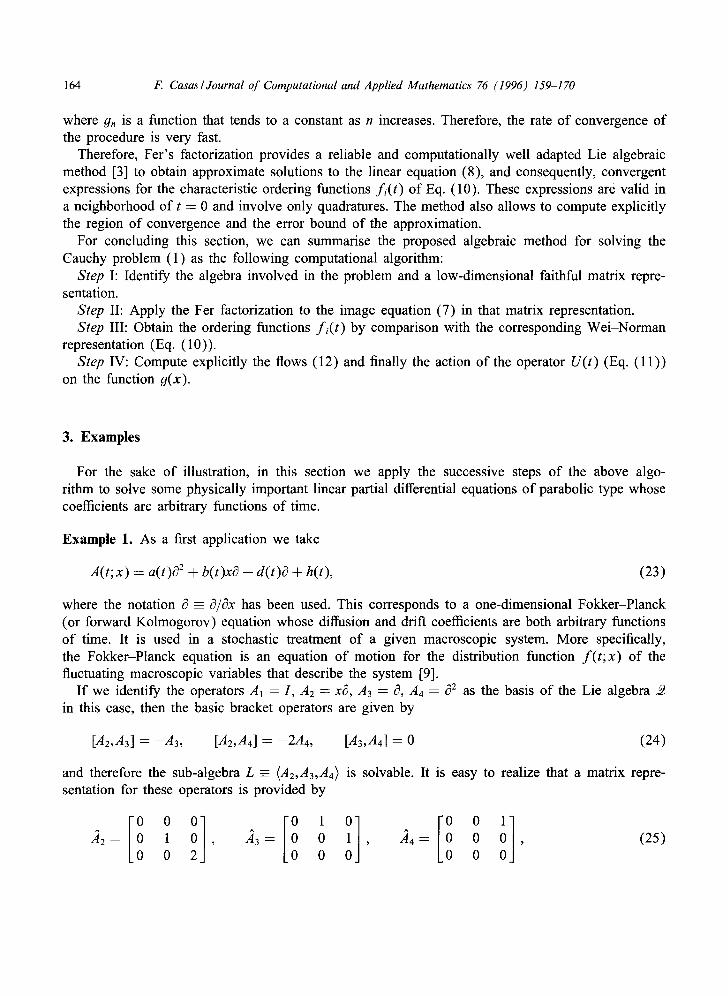
where 9n is a function that tends to a constant as n increases. Therefore, the rate of convergence of the procedure is very fast.

Therefore, Fer's factorization provides a reliable and computationally well adapted Lie algebraic method [3] to obtain approximate solutions to the linear equation (8), and consequently, convergent expressions for the characteristic ordering functions fi(t) of Eq. (10). These expressions are valid in a neighborhood of t = 0 and involve only quadratures. The method also allows to compute explicitly the region of convergence and the error bound of the approximation.

For concluding this section, we can summarise the proposed algebraic method for solving the Cauchy problem (1) as the following computational algorithm:

Step I: Identify the algebra involved in the problem and a low-dimensional faithful matrix repre- sentation.

Step II: Apply the Fer factorization to the image equation (7) in that matrix representation. Step III: Obtain the ordering functions fi(t) by comparison with the corresponding Wei-Norman

representation (Eq. (10)). Step IV: Compute explicitly the flows (12) and finally the action of the operator U(t) (Eq. (11 ))

on the function 9(x).

3. Examples

For the sake of illustration, in this section we apply the successive steps of the above algo- rithm to solve some physically important linear partial differential equations of parabolic type whose coefficients are arbitrary functions of time.

Example 1. As a first application we take

A(t;x) = a(t)02 + b(t)xO ÷ d(t)O + h(t), (23)

where the notation 0 _-- 0/0x has been used. This corresponds to a one-dimensional Fokker-Planck (or forward Kolmogorov) equation whose diffusion and drift coefficients are both arbitrary functions of time. It is used in a stochastic treatment of a given macroscopic system. More specifically, the Fokker-Planck equation is an equation of motion for the distribution function f( t;x) of the fluctuating macroscopic variables that describe the system [9].

If we identify the operators A1 = I, A2 = x0, A3 = 0, A4 = 02 as the basis of the Lie algebra in this case, then the basic bracket operators are given by

[A:2,A3] = - A 3 , [A2,A4] = - 2 A 4 , [A3,A4] = 0 (24)

and therefore the sub-algebra L =-- (Az,A3,A4) is solvable. It is easy to realize that a matrix repre- sentation for these operators is provided by

[i°il [°li] [i°i] A2---- 1 , 23---- 0 0 , ~z~4---- 0 , 0 0 0 0

(25)

F.. Casas / Journal of Computational and Applied Mathematics 76 (1996) 159-170 165

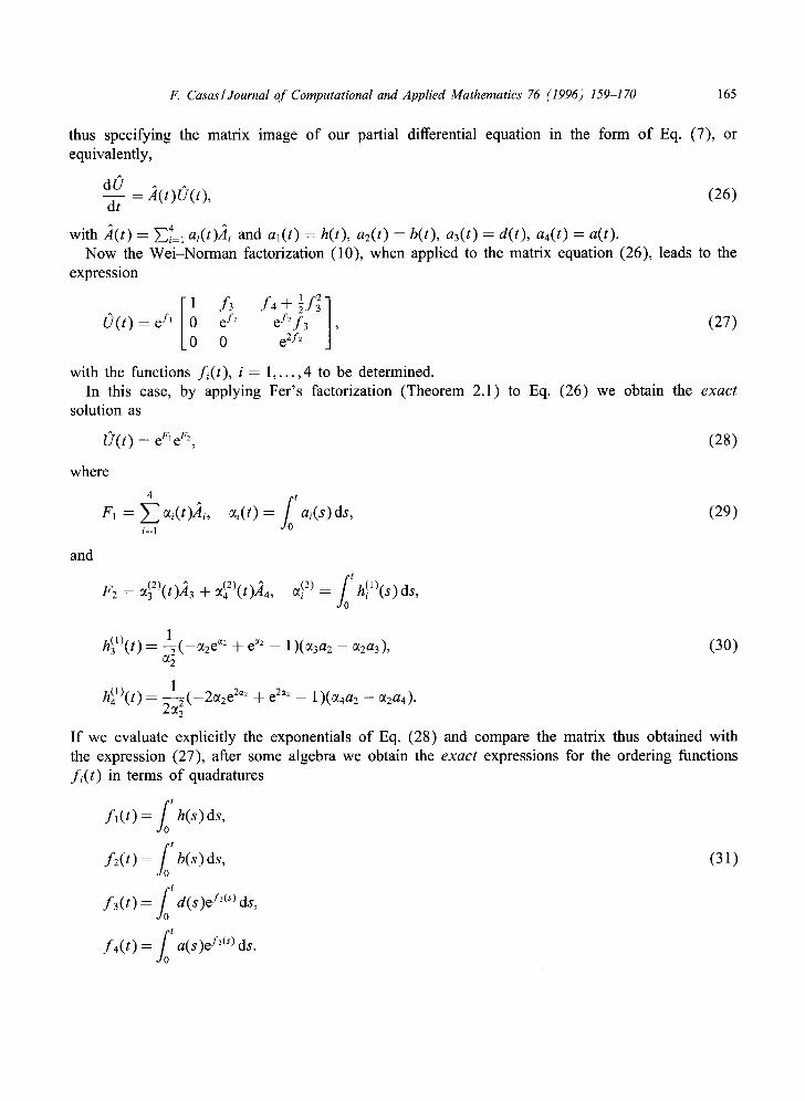
thus specifying the matrix image of our partial differential equation in the form of Eq. (7), or equivalently,

dO - - ~ 4 ( t ) O ( t ) , (26)

dt

with ~i(t) 4 ^ = ~i=1 ai(t)Ai and al(t) = h(t), a2(t) = b(t), a3(t) = d(t), a4(t) = a(t). Now the Wei-Norman factorization (10), when applied to the matrix equation (26), leads to the

expression

U ( t ) = e f ' 0 e f : e J 2 f 3 , ( 2 7 )

0 0 e af2

with the functions f ,( t) , i = 1 , . . . ,4 to be determined. In this case, by applying Fer's factorization (Theorem 2.1) to Eq. (26) we obtain the exact

solution as

U(t) = eF'e F2, (28)

where

4 F1 = Z ~i(t)f4i,

i=l ~0 t ~i(t) = ai(s) ds, (29)

and

F 2 = ~2)(t)/13 ~- 0~2)(/)~z]4, ~0 t o¢~ 2) = hl l ) ( s )ds ,

h~l)(t) = 1- ~-~2e~2 + e ~2 - 1)(~3a2 - - ~2a3), (30)

h~l)(t)_ - 1 (-2~2e2~2 + e2~2 2 ~ - - 1 ) ( ~ 4 a 2 - - c~2a4).

If we evaluate explicitly the exponentials of Eq. (28) and compare the matrix thus obtained with the expression (27), after some algebra we obtain the exact expressions for the ordering functions f i ( t ) in terms of quadratures

/0t f l (t) = h(s) ds,

fOt f 2 ( t ) = b ( s )d s , (31)

f3( t ) = J/a't d(s)eZ2(s) ds,

/0 t f 4 ( t ) = a(s)e z2(') ds.

166 F. Casasl Journal of Computational and Applied Mathematics 76 (1996) 159-170

The same expressions can be obtained, of course, by writting down and solving the differential equations satisfied by the functions f~(t) [14]. This is possible here because the Lie algebra involved is solvable.

Finally, by using the easily derivable expressions [11, 14]

r a l exp[a(t)X ~x I 9(x) = 9 (ea(')x), (32)

exp [a(t)~x I 9(x)=9(x+ a( t ) ) , (33)

exp # ( x ) - J - ~ exp 9(y)dy, (34)

we find for f(t;x),

ef'(') / / ~ [ -[y-(xef2m+f3(t ) )]2 t > O , (35) f(t;x) -- 4x/~f4(t ) ~ dyy(y) exp 4fa(t) '

a result previously obtained in [11, 14] with different algebraic techniques.

Example 2. Next we consider the operator A(t;x) given by

A(t;x) = a ( t ) c 32 q- b(t)xO + c(t)x 2, (36)

where a(t), b(t), c(t) are complex valued bounded analytic functions. This constitutes a generalization of a linear Fokker-Planck equation. If we denote

2 I 2 ( 3 7 ) A~ = / , Ae = ¼(1 + 2x0), A3 = ix , A4 = ~c3 ,

then these operators form a basis of the Lie algebra .~, the basic bracket relations are

[Az,A3] = A3, [A2,A4] = - A 4 , [A3,A4] = - A 2 (38 )

and the sub-algebra (Az,A3,A4> can be identified with SU(1,1), which is not solvable. A matrix representation of the SU(1, 1) generators is provided by

,[; ,[°°01 ,39, 4 2 = 5 -- ' 0 0 ' = ~ 1 '

and the image of the operator A(t;x) under this representation can be written as Eq. (9) with al(t) = -lb(t), a2(t) = 2b(g), a3(t) = 2c(t), a4(t) = 4a(t).

If we apply the Wei-Norman factorization to the linear equation (8), the corresponding solution can be now represented as

- ef2/2(1 -- ] ½/3f4) --f3e f2/2 U(t) = e f' (40) ] 1 ¢ ~-f2/2 e-f2/2

~J4 ~

in a neighborhood of t = 0. In this case the system of differential equations that determine the functions fi cannot be solved by quadratures for arbitrary coefficients ai(t) [4]. Nevertheless, Fer's

F. Casasl Journal of Computational and Applied Mathematics 76 (1996) 159-170 167

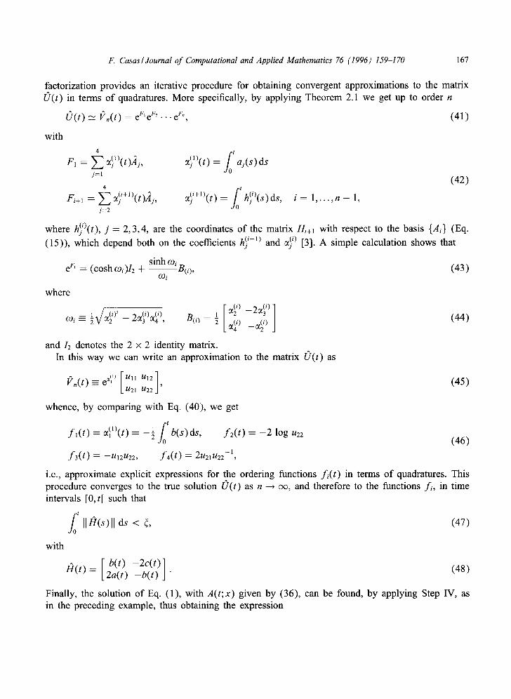
factorization provides an iterative procedure for obtaining convergent approximations to the matrix U(t) in terms of quadratures. More specifically, by applying Theorem 2.1 we get up to order n

with

U(t) ~ l~n(t) = eFte F2 ' ' ' e F", (41)

4 t

F1 = Z ~5~)(t)]~' ' ~51)(t) = fo a,(s)ds /=1 (42)

4 t

Fi+l = ~ ~5++l)(t)Aj, ~i+l)(t) = fo hSO(s)ds' i = 1 , . . . , n - 1, j=2

where hy)(t), j = 2,3,4, are the coordinates of the matrix Hi+ 1 with respect to the basis {Ai} (Eq. (15)), which depend both on the coefficients h5 i-1) and a5 i) [3]. A simple calculation shows that

e F' (coshooi)I2 + sinh~oi = B(0 , (43) fDi

where

1 ~/0{(i)2 .(i) .(0 1 [ ~ 0 --20~I 0- -- -- 2% a 4 , __~i) (44)

and /2 denotes the 2 x 2 identity matrix. In this way we can write an approximation to the matrix /)(t) as

I)n(t)-----e'~") [ ullu2, u22U12] , (45)

whence, by comparing with Eq. (40), we get

/0' 1 b(s) ds, f2(t) = - 2 log U22 f l ( t ) = ~]l)(t) = - 5 (46)

f3(t) = --U12U22, f4(t) = 2U21U22 - 1 ,

i.e., approximate explicit expressions for the ordering functions ft.(t) in terms of quadratures. This procedure converges to the true solution U(t) as n --+ cxz, and therefore to the functions fi, in time intervals [0, t[ such that

f ' II II < 4, (47) & s ) ds

with

H(t) = [ : ( ;~) -2c(t)_b(t) ]" ] (48)

Finally, the solution of Eq. (1), with A(t;x) given by (36), can be found, by applying Step IV, as in the preceding example, thus obtaining the expression

168 F. Casas / Journal of Computational and Applied Mathematics 76 (1996) 159 170

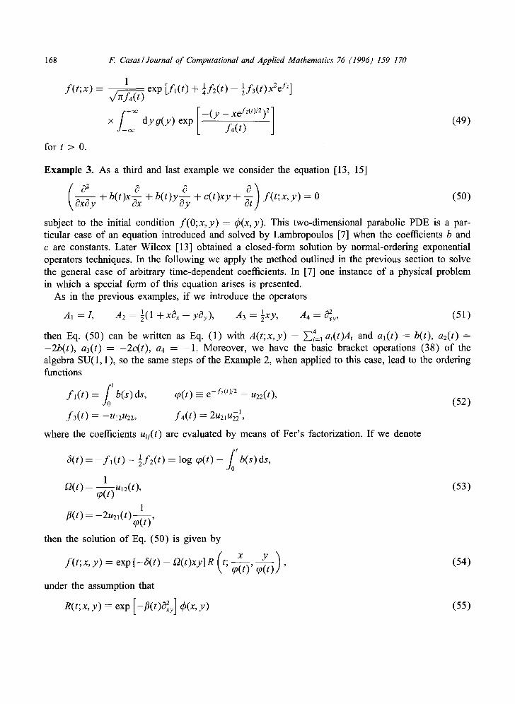
1 f ( t ; x ) --

x/.f4(t) r 1 1 2 f2 exp [f l( t ) + ~f2(t) + 5 f 3 ( t ) x e ]

for t > 0.

f ~O(2

× d y g ( y ) exp oo

_ ( y _ x e f 2 ( t ) / 2 ) 2

f4(t) (49)

f 0 t 6 ( t ) = - f l ( t ) - ½f2( t )= log q~(t)- b(s)ds ,

1 =

I fl(t) = -2u21(t) o(t),

then the solution of Eq. (50) is given by

( x y ) f ( t ; x , y ) = e x p [ - 6 ( t ) - (2( t )xy]R t; ~o(t)' ~p(t) '

under the assumption that

R(t;x, y ) = exp [-fl(t)#~y] dp(x, y )

(53)

(54)

(55)

Example 3. As a third and last example we consider the equation [13, 15]

~ + b ( t ) x + b ( t ) y + c ( t ) x y + ~ f ( t ; x , y ) = 0 (50)

subject to the initial condition f (0 ;x , y) = qS(x, y). This two-dimensional parabolic PDE is a par- ticular case of an equation introduced and solved by Lambropoulos [7] when the coefficients b and c are constants. Later Wilcox [13] obtained a closed-form solution by normal-ordering exponential operators techniques. In the following we apply the method outlined in the previous section to solve the general case of arbitrary time-dependent coefficients. In [7] one instance of a physical problem in which a special form of this equation arises is presented.

As in the previous examples, if we introduce the operators

At = I , A2 ½(1 + XC3x + yC~y), A3 1 2 = = 5xy, A4 = C~xy, (51)

then Eq. (50) can be written as Eq. (1) with A ( t ; x , y ) = ~=1 ai(t)Ai and al( t) = b(t), a2(t) = -2b( t ) , a3(t) = -2c( t ) , a4 = -1 . Moreover, we have the basic bracket operations (38) of the algebra SU(1, 1 ), so the same steps of the Example 2, when applied to this case, lead to the ordering functions

/0' f l ( t ) = b(s) ds, qo(t) =- e -f2(t)/2 = u22(t), (52)

f3( t ) = -UlzU22, f4( t ) = 2uzlu51,

where the coefficients uij(t) are evaluated by means of Fer's factorization. If we denote

F. Casas / Journal of Computational and Applied Mathematics 76 (1996) 159-170 169

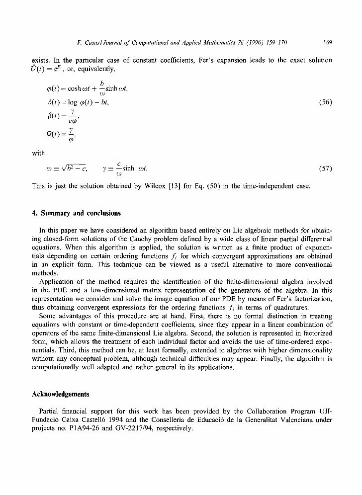
exists. In the particular case of constant coefficients, Fer's expansion leads to the exact solution U ( t ) = e v ' , o r , equivalently,

~p(t) = cosh cot + bs inh cot, co

~(t) = log qg(t) - bt,

fl(t) = 7 , cq~

f2(t) 7 q9

(56)

with

co ---- x / ~ - c, ~ - Csinh cot. co

This is just the solution obtained by Wilcox [13] for Eq. (50) in the time-independent case.

(57)

4. Summary and conclusions

In this paper we have considered an algorithm based entirely on Lie algebraic methods for obtain- ing closed-form solutions of the Cauchy problem defined by a wide class of linear partial differential equations. When this algorithm is applied, the solution is written as a finite product of exponen- tials depending on certain ordering functions fg for which convergent approximations are obtained in an explicit form. This technique can be viewed as a useful altemative to more conventional methods.

Application of the method requires the identification of the finite-dimensional algebra involved in the PDE and a low-dimensional matrix representation of the generators of the algebra. In this representation we consider and solve the image equation of our PDE by means of Fer's factorization, thus obtaining convergent expressions for the ordering functions f,. in terms of quadratures.

Some advantages of this procedure are at hand. First, there is no formal distinction in treating equations with constant or time-dependent coefficients, since they appear in a linear combination of operators of the same finite-dimensional Lie algebra. Second, the solution is represented in factorized form, which allows the treatment of each individual factor and avoids the use of time-ordered expo- nentials. Third, this method can be, at least formally, extended to algebras with higher dimensionality without any conceptual problem, although technical difficulties may appear. Finally, the algorithm is computationally well adapted and rather general in its applications.

Acknowledgements

Partial financial support for this work has been provided by the Collaboration Program UJI- Fundaci6 Caixa Castell6 1994 and the Conselleria de Educaci6 de la Generalitat Valenciana under projects no. P 1 A94-26 and GV-2217/94, respectively.

170 E Casas / Journal of Computational and Applied Mathematics 76 (1996) 159-170

References

[1] J.G.F. Belinfante and B. Kolman, A Survey of Lie Groups and Lie Algebras with Applications and Computational Methods (SIAM, Philadelphia, 1972).

[2] S. Blanes, Evolution of dynamical systems: magnus and fer expansions, Master Thesis, Universitat de Val6ncia, 1994.

[3] F. Casas, Fer's factorization as a symplectic integrator, Numer. Math. 74 (1996) 283-303. [4] G. Dattoli, M. Richetta, G. Schettini and A. Torre, Lie algebraic methods and solutions of linear partial differential

equations, J. Math. Phys. 31 (1990) 2856-2863. [5] F. Fer, R6solution de l'equation matricielle O = pU par produit infini d'exponentielles matricielles, Bull. Classe Sci.

Acad. Roy. Belg. 44 (1958) 818-829. [6] R. Gilmore, Lie Groups, Lie Algebras, and Some of Their Applications (Krieger, Malabar, FL, 1994). [7] P. Lambropoulos, Solution of the differential equation (~2/(~xOy 4- ax(t~/t~x) 4- by(~/Oy) + cxy + ~/~t)P = O, J. Math.

Phys. 8 (1967) 2167-2169. [8] P.J. Olver, Applications of Lie Groups to Differential Equations (Springer, New York, 2nd ed., 1993). [9] H. Risken, The Fokke~Planck Equation (Springer, Berlin, 2nd ed., 1989).

[10] S. Steinberg, Applications of the Lie algebraic formulas of Baker, Campbell, Hausdorff and Zassenhaus to the calculation of explicit solutions of partial differential equations, J. Differential Equations 26 (1977) 404-434.

[11] M. Suzuki, Decomposition formulas of exponential operators and Lie exponentials with some applications to quantum mechanics and statistical physics, J. Math. Phys. 26 (1985) 601-612.

[12] J. Wei and E. Norman, On global representations of the solutions of linear differential equations as a product of exponentials, Proc. Amer. Math. Soc. 15 (1964) 327-334.

[13] R. Wilcox, Closed-form solution of the differential equation (O2/~xOy + ax(O/~x) + by(8/Oy) + cxy + (~/Ot))P -- 0 by normal-ordering exponential operators, J. Math. Phys. 11 (1970) 1235-1237.

[14] F. Wolf, Lie algebraic solutions of linear Fokker-Planck equations, J. Math. Phys. 29 (1988) 305-307. [15] D. Zwillinger, Handbook of Differential Equations (Academic Press, Boston, 2nd ed., 1992).