Solution of impact tasks, assessment of result reliability M. Okrouhlík Institute of...

Solution of impact tasks,assessment of result reliability

M. Okrouhlík

Institute of Thermomechanics

Scope of the lecture

• What is a ‘good agreement’ in dynamical transient analysis in solid continuum mechanics

• Vehicle for comparison• Continuum model and its limits• Experimental and FE analysis• Assessment of agreement quality• Synergy of FE and experimental analyses• Conclusions

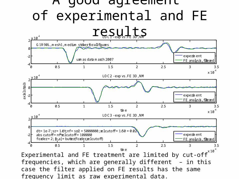
A good agreement of experimental and FE results

0 0.5 1 1.5 2 2.5 3 3.5

x 10-4

-4

-2

0

2x 10

-4 LOC1 - exp vs. FE 3D, NM

G1R90L, mesh1, medium striker for all figures

urmas data march 2007

experimentFE analysis, filtered

0 0.5 1 1.5 2 2.5 3 3.5

x 10-4

-4

-2

0

2x 10


axi

al s

tra

in

time


0 0.5 1 1.5 2 2.5 3 3.5

x 10-4

-4

-2

0

2x 10


time

dt = 1e-7; sr = 1/dt; nf = sr/2 = 5000000; rel cut off = 1/50 = 0.02abs cut off = nf*rel cut off = 100000f order = 2; [b,a] = butter(f order,rel cut off)


Experimental and FE treatment are limited by cut-off frequencies, which are generally different – in this case the filter applied on FE results has the same frequency limit as raw experimental data.

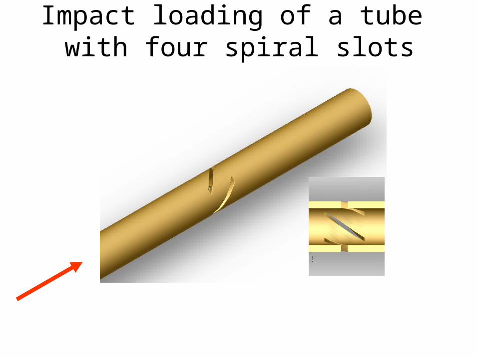
Impact loading of a tube with four spiral slots

Dimensions and points of interest

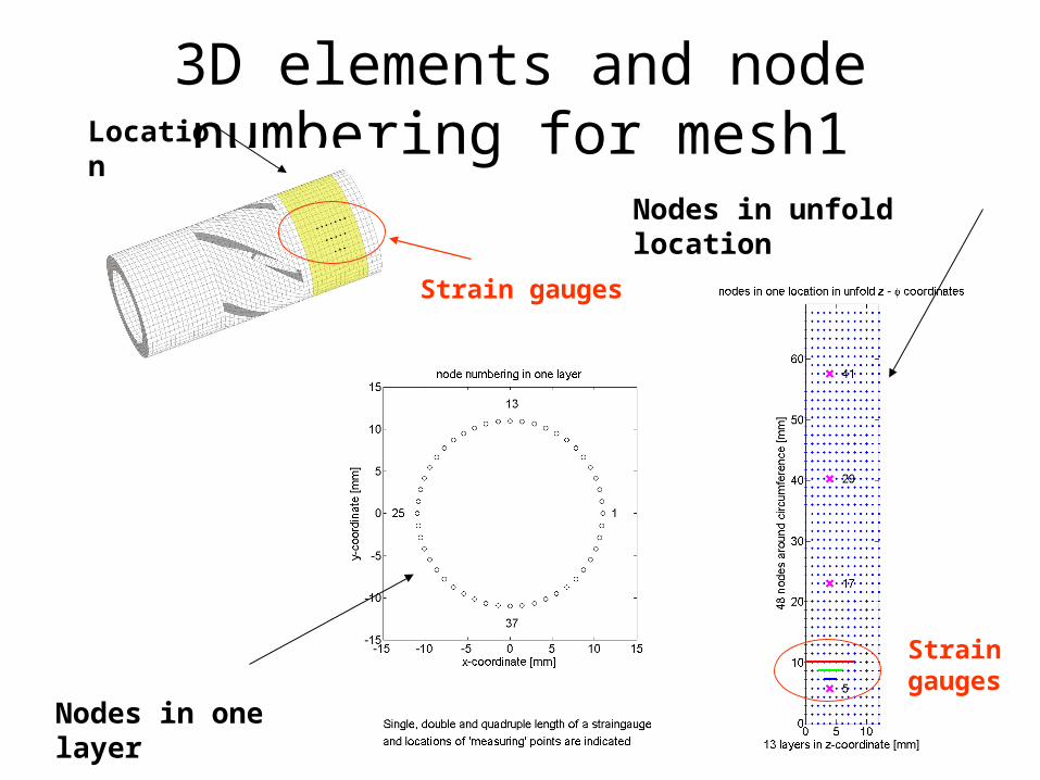
3D elements and node numbering for mesh1

Nodes in unfold location

Nodes in one layer

Location

Strain gauges

Strain gauges

Geometry, material and elements

G1R90L_NM ... four slots with 15 deg. indentation, axial length = 17.28 mm, slots and mesh rotate 90 deg

Geometry and elements first part of the tube = 800 mm 800 layers, 144 elem in one layer

second part, ie. axial length of slots = 17.28 mm 18 layers, 120 elem in one layerthird part of the tube = 800 mm 800 layers, 144 elem in one layertotal lenght of tube = 1617.28 mm 1618 total number of layersouter to inner diameters D/d = 22/16 mmnumber of spiral slots = 4

Element propertiestrilinear bricks elements, 8 nodes, Gauss order quadrature NG = 3consistent mass matrix for NM (Newmark)diagonal mass matrix for CD (central differences)number of elements 232 560number of nodes 310 576number of degrees of freedom 931 728max. front width 606

Material propertiesYoung modulus = 2.05e11 PaPoisson's ratio = 0.24density = 7800 kg/m^3

Loading and FE technologyLoading

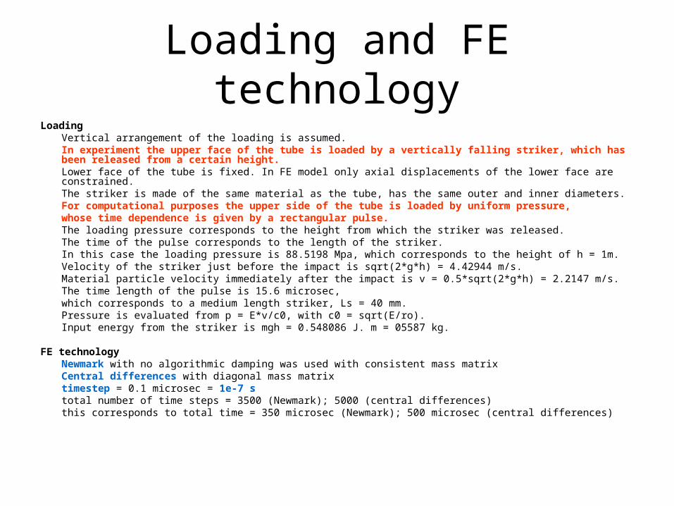
Vertical arrangement of the loading is assumed.In experiment the upper face of the tube is loaded by a vertically falling striker, which has been released from a certain height.Lower face of the tube is fixed. In FE model only axial displacements of the lower face are constrained.The striker is made of the same material as the tube, has the same outer and inner diameters.For computational purposes the upper side of the tube is loaded by uniform pressure,whose time dependence is given by a rectangular pulse.The loading pressure corresponds to the height from which the striker was released.

The time of the pulse corresponds to the length of the striker.In this case the loading pressure is 88.5198 Mpa, which corresponds to the height of h = 1m.Velocity of the striker just before the impact is sqrt(2*g*h) = 4.42944 m/s.Material particle velocity immediately after the impact is v = 0.5*sqrt(2*g*h) = 2.2147 m/s.The time length of the pulse is 15.6 microsec,

which corresponds to a medium length striker, Ls = 40 mm.Pressure is evaluated from p = E*v/c0, with c0 = sqrt(E/ro).Input energy from the striker is mgh = 0.548086 J. m = 05587 kg.

FE technologyNewmark with no algorithmic damping was used with consistent mass matrixCentral differences with diagonal mass matrixtimestep = 0.1 microsec = 1e-7 stotal number of time steps = 3500 (Newmark); 5000 (central differences)this corresponds to total time = 350 microsec (Newmark); 500 microsec (central differences)

Wavefront timetable

FE strain distribution in location 1

Raw comparison – no tricks

0 1 2 3 4 5 6

x 10-5

-4

-3

-2

-1

0

1

2x 10

-4 LOC0 - exp vs. FE axisym, CD

axia

l str

ain

mesh1, medium striker for all figures

urmas data march 2007

0 0.5 1 1.5 2 2.5 3 3.5

x 10-4

-4

-3

-2

-1

0

1

2x 10


0 0.5 1 1.5 2 2.5 3 3.5

x 10-4

-4

-3

-2

-1

0

1

2x 10


axia

l str

ain

time

0 0.5 1 1.5 2 2.5 3 3.5

x 10-4

-4

-3

-2

-1

0

1

2x 10


time

experiment

FE analysis

experiment

FE analysis

experiment

FE analysis

experiment

FE analysis

Are FE or experimental results closer to reality? Where is the truth?

Where is the truth? Are experimental or FE results closer to reality?

• When trying to reveal the ‘true’ behavior of a mechanical system we are using the experiment

• When trying to predict the ‘true’ behavior of a mechanical system we are accepting a certain model of it and then solve it analytically and/or numerically

• Physical laws (models) as– Newton’s – Energy conservation– Theory of relativity

cannot be proved (in mathematical sense)

• Often we say that it is the experiment which ultimately confirms the model

• But experiments, as well as the numerical treatment of models describing the nature, have observational thresholds. Sometimes, the computational threshold of computational analysis are narrower than those of experiment

• Let’s ponder about limits of applicability of continuum model as well as about limits of modern computational approaches when applied to approximate solution of continuum mechanics

Continuum mechanics

• Deals with response of solid and/or fluid medium to external influence

• By response we mean description of motion, displacement, force, strain and stress expressed as functions of time and space

• By external influence we mean loading, constraints, etc. Expressed as functions of time and space

Solid continuum mechanics

• Macroscopic model disregarding the corpuscular structure of matter

• Continuous distribution of matter is assumed – continuity hypothesis

• All considered material properties within the observed infinitesimal element are identical with those of a specimen of finite size

• Quantities describing the continuum behaviour are expressed as piecewice continuous functions of time and space

Governing equations

• Cauchy equations of motion

• Kinematic relations

• Constitutive relations

itt

it

jtji

tt xfx

j

kt

i

kt

i

jt

j

it

ij x

u

x

u

x

u

x

u00002

1angeGreen_Lagr

i

jt

j

it

ij x

u

x

u002

1eng

engengklijklij C Lagrange_Green

klijklij DS

For transient problems, we are interested in, the inertia forces are to be taken into account

In linear continuum mechanicsthe equations are simplified to

klijkliji

j

j

iij

ii

j

ji Cx

u

x

u

t

uf

x

,2

1,

2

2

• Inertia forces are considered

• loading is

• localized in space

• of short duration with a short rise time

The high frequency components are of utmost importance

Wave equation 2D - plane stress, Lamé equations – expressed in displacements only

,1

2

2

22

2

2

22

2

xy

v

y

uG

yx

v

x

uE

t

u

.1

2

2

22

2

2

22

2

yx

u

x

vG

yx

u

y

vE

t

v

tcxfu 3

tcyhv 3 tcyFu 2

tcxHv 2

23 1

Ec

G

c 2 S … shearP … primary

Longitudinaldilatationalirrotationalextension

Transversalshearrotationaldistortionequivolumetrical

Nondispersive and uncoupled solutions in unbound region

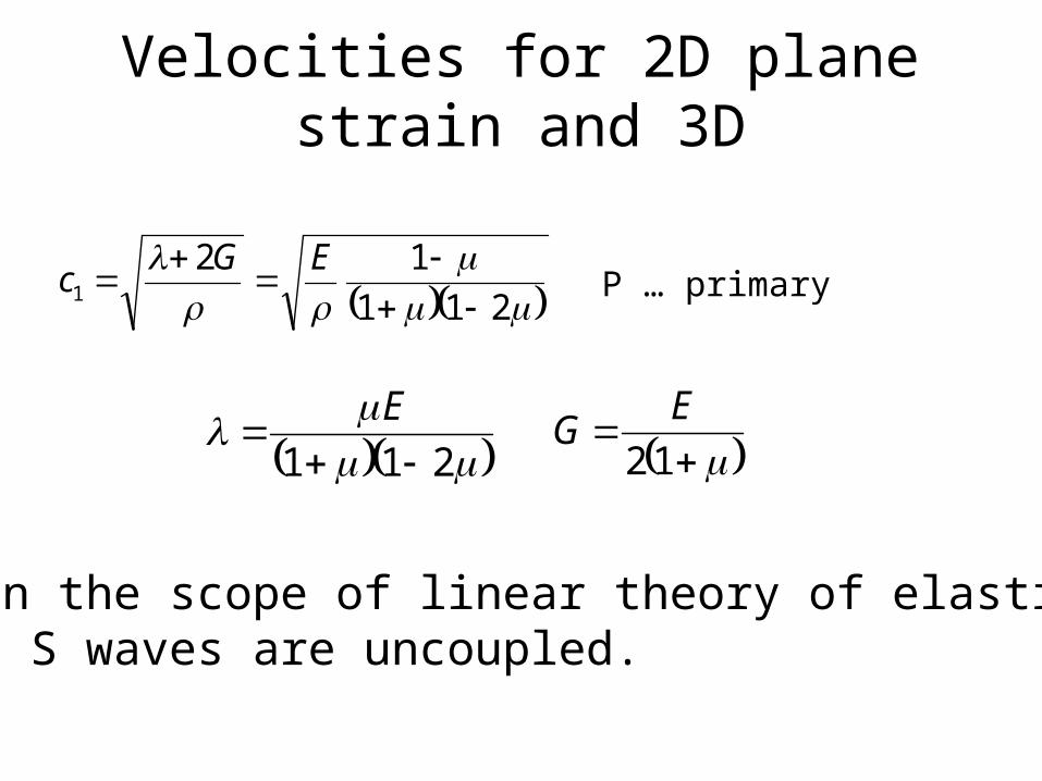
Velocities for 2D plane strain and 3D

211

121

EGc

211

E 12

EG

P … primary

Within the scope of linear theory of elasticity,P and S waves are uncoupled.

Typical values for steel in m/s

For E = 2.1e11 Pa, = 7800 kgm^-3, = 0.3

0.3for Rayleigh wave,R29849274.0

stress planefor waveP5439))1(/(

shear wave,S3218/

3D strain, planefor waveP6020/)2(

barslender wave,D15189/

2R

23

2

1

0

cc

Ec

Gc

Gc

Ec

Analytical solutions for bounded regions are difficult and exist

for bodies with simple initial and boundary conditions only

One way to solve the problem is to apply the Fourier transform in space and the Laplace transform in time on equations of motion. The subsequent inverse procedure leads to infinite series of improper integrals.

To indicate amount of effort to be exerted, the formulas derived by F. Valeš are shown.

A typical expression for a stress component

in a transiently loaded thin elastic strip is shown

Relations between integrand quantities and integral variable

Roots of these so called dispersive relations have to be evaluated numerically before the integration itself.

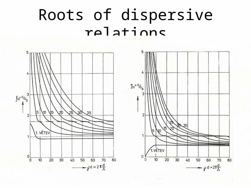
Roots of dispersive relations

After all, the analytical solution ends up

with a numerical evaluation

• Only finite number of terms can be summed up• Integration itself has to be provided numerically

• This led to development of approximate numerical solutions

Today, approximate methods of solution prevail Discretization Finite difference method Transfer matrix method Matrix method Displacement formulation Force formulation Finite element method Displacement formulation Force formulation Hybrid finite element method Mixed finite element method

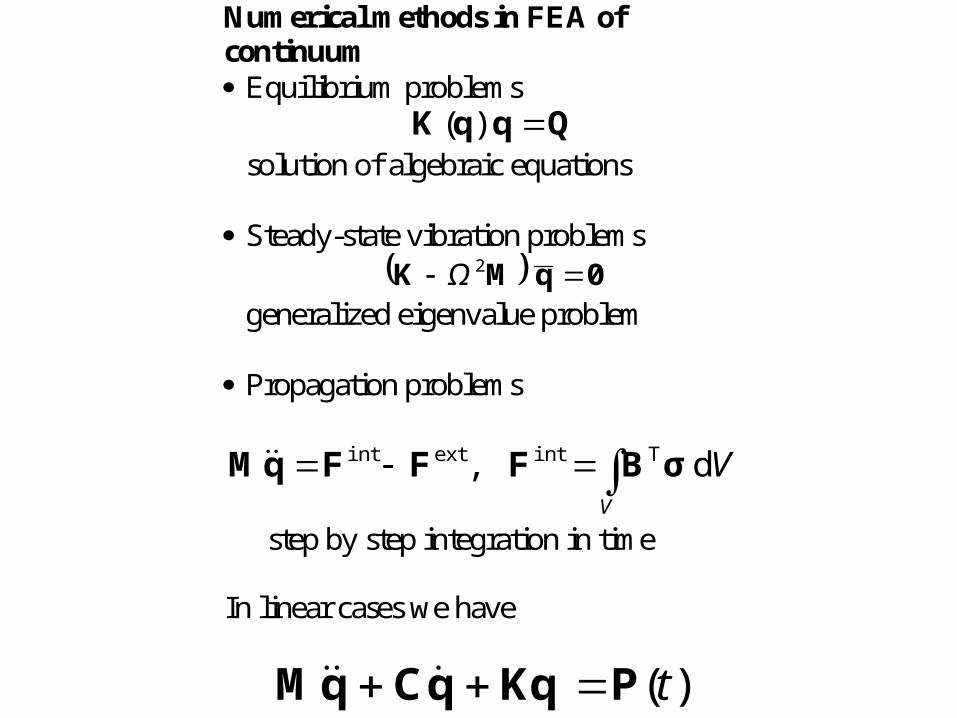
Numerical methods in FEA of continuum Equilibrium problems

QqqK )( solution of algebraic equations Steady-state vibration problems

0qMK 2Ω generalized eigenvalue problem Propagation problems

VV

d, Tintextint σBFFFqM

step by step integration in time In linear cases we have

)(tPKqqCqM

Unbound frequency response of continuum

For fast transient problems as shock and impact the high frequency components of solutions are of utmost importance. In continuum, there is no upper limit of the frequency range of the response. In this respect continuum is able to deal with infinitely high frequencies. This is a sort of singularity deeply embedded in the continuum model.

As soon as we apply any of discrete methods for the approximate treatment of transient tasks in continuum mechanics, the value of upper cut-off frequency is to be known in order to ‘safely’ describe the frequencies of interest.

Dispersive propertiesof 1D and 2D constant strain elements

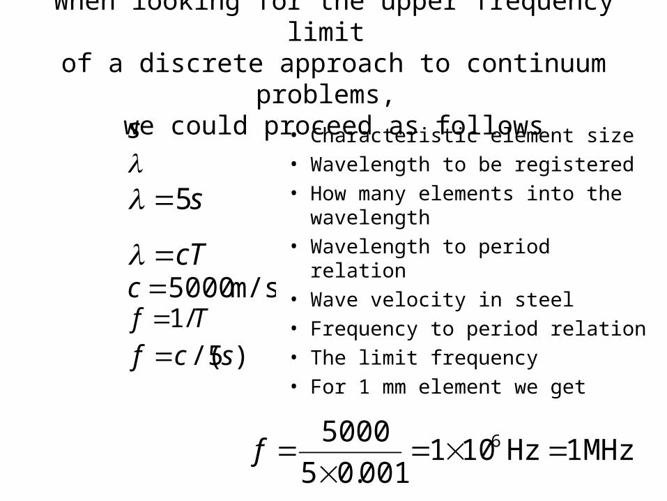
When looking for the upper frequency limit of a discrete approach to continuum problems,

we could proceed as follows

• Characteristic element size• Wavelength to be registered• How many elements into the

wavelength• Wavelength to period relation• Wave velocity in steel• Frequency to period relation• The limit frequency• For 1 mm element we get

s

s5

m/s5000ccT

Tf /1)5/( scf

MHz 1 Hz101001.05

5000 6

f

10-10

10-8

10-6

10-4

10-2

10-2

100

102

104

106

108

size in [m]

freq

uenc

y in

[Mhz

]

characteristic sizes and corresponding frequencies

atom sizeaustenite steel grain size1 mm finite element1 MHz level1 GHz levelFE analysis range from 0.1mm to 100mmmaximum exp. sampling limit 100 MHz - 14 bits

Where is the continuum limit?

Limits of continuum, FE analysis and experiment

Validity limits of a model

• Model is a purposefully simplified concept of a studied phenomenon invented with the intention to predict – what would happen if ..

• Accepted assumptions (simplifications) specify the validity limits of the model

• Model is neither true nor false

• Regardless of being simple or complicated, it is good, if it is approved by an experiment

Using a model outside its limits is a blunder

• Using a model outside of its validity limits leads to erroneous results and conclusions

• This is not, however, the fault of the model, but pure consequence of a poor judgment of the model’s user

• Model gives no warning. Lot of checks might be satisfied and still …

Blunders are easy to commit

• Point force is– prohibited in continuum,– frequently used in FE analysis

• Employing smaller and smaller elements, leads to singularity, since we are coming closer and closer to ‘continuum’ revealing thus unacceptable behavior of the point force in continuum

• An example follow

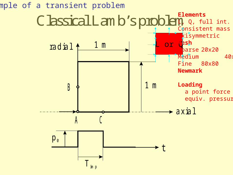
Classical Lamb’s problem

ra d ia l

B

A C

1 m

1 m

a xia l

p 0

T im p

t

L or Q

ElementsL, Q, full int.Consistent massaxisymmetricMeshCoarse 20x20Medium 40x40Fine 80x80Newmark

Loading a point force equiv. pressure

Example of a transient problem

Primary wave

Lamb, presure loading, rectangular pulse, velocity distribution, FEA

P waves

S waves

R waves

Again, where is the first nonzero P-wave appearance?

Pollution-free energy production

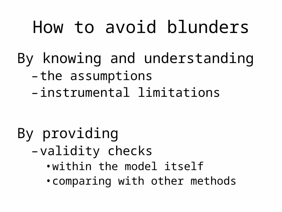
How to avoid blunders

By knowing and understanding– the assumptions– instrumental limitations

By providing– validity checks

• within the model itself• comparing with other methods

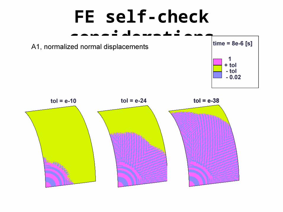
FE self-check considerations

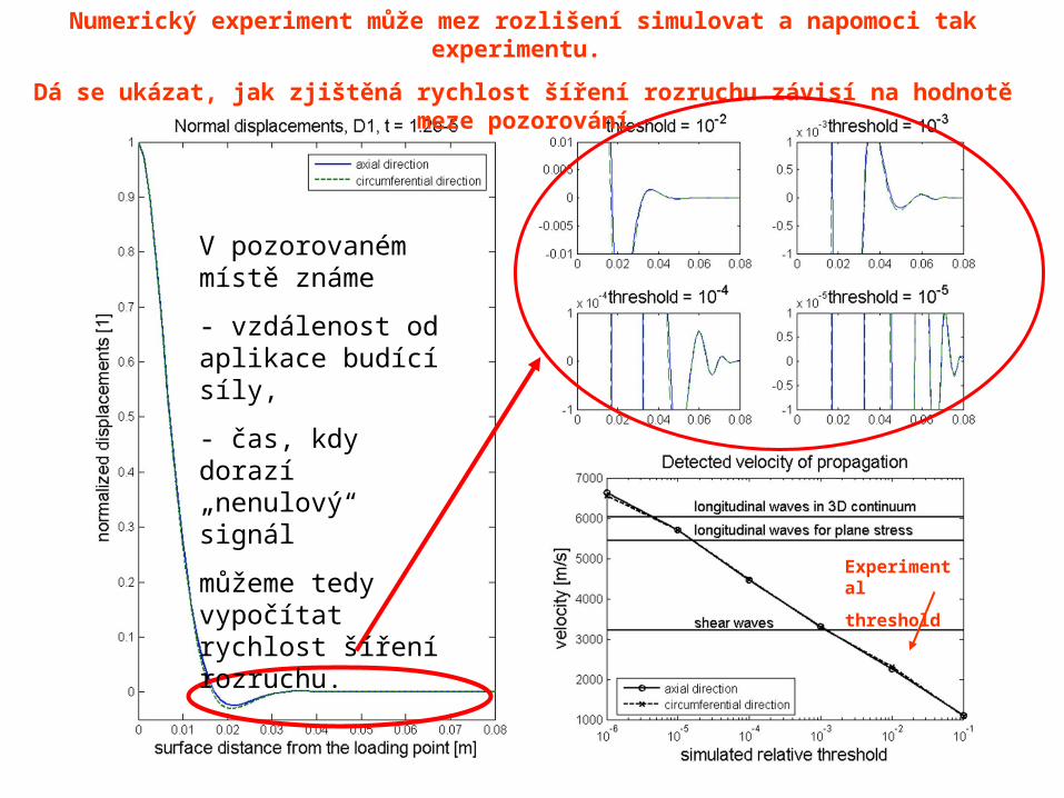
Numerický experiment může mez rozlišení simulovat a napomoci tak experimentu.

Dá se ukázat, jak zjištěná rychlost šíření rozruchu závisí na hodnotě meze pozorování

Experimental

threshold

V pozorovaném místě známe

- vzdálenost od aplikace budící síly,

- čas, kdy dorazí „nenulový“ signál

můžeme tedy vypočítat rychlost šíření rozruchu.

Numerical analysis should be robust

It should inform us about its limits

Should be independent of – mass matrix formulation– the method of integration– meshsize– element type

It is not always so, very often our results are method dependent. See the next example.

Validity self-assessments, NM vs. CD

C o m p u t a t i o n a l i n f i n i t e s p e e d o f w a v e p r o p a g a t i o n c a n b e e x p l a i n e d b y a n a l y z i n g t h e t i m e m a r c h i n g a l g o r i t h m s f o r tPKqqM

E x p l i c i t ( c e n t r a l d i f f e r e n c e s ) I m p l i c i t ( N e w m a r k ) E q u i l i b r i u m i s c o n s i d e r e d a t t i m e t tt a n d l e a d s t o r e p e a t e d s o l u t i o n s o f

ttttPMq~

2

1 tttt PqK ˆˆ

b o u n d edn o t is np ro p ag atio o f sp eed n alco mp u tatiod iag o n alb en ev ercan

d iag o n al is ifo n ly d iag o n al,isfu ll;b an d ed ;g en erally 1

K

MMMKMK 11

ˆ,,

ttttt tt

MqqMKPP

22

22~ MKK2

1

t

ˆ

ttttttt ccc qqqMPP 321 ˆ

Instrumental limitation

Floating point representation of real numbers threshold

Memory size limitation

Meshsize and time step limitations

machine epsilon

FFT frequency analysis

Now, let’s concentrate on the frequency analysis frequency analysis of the loading pulse and of axial and radial displacements obtained in the outer corner node of location C by means of NM and CD operators for the mesh1. The normalized power spectra are plotted in the range from 0 to Nyquist frequency together with the power spectrum of the loading pulse.

timestep [s] sampling rate [MHz] Nyquist frequency [MHz]mesh1 1e-7 10 5mesh2 1e-7/2 20 10 mesh3 1e-7/4 40 20 mesh4 1e-7/8 80 40

Assessment by frequency analysis

0 1 2 3 4

x 10-5

0

0.5

1

1.5

2

2.5x 10

4 imput pulse

time0 1 2 3 4

x 10-5

0

1

2

3

x 10-5 mesh1, disp, corner node

time

0 0.5 1 1.5 2 2.5 3 3.5 4 4.5 5

x 106

0

1

2

3

4

5

6x 10

-10

frequency from 0 to Nyquist

transfer function, input vs. rad. disp

radial NMaxial NMradial CDaxial CD

NMCDbreathing frequencyzig-zag L frequencyzig-zag S frequencyFE limit frequency consFE limit frequency diag

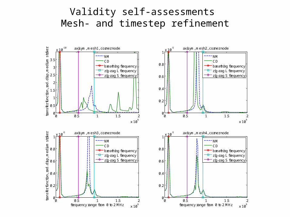
Validity self-assessments Mesh- and timestep refinement

0 0.5 1 1.5 2

x 106

0

0.5

1

1.5

2

2.5

3

3.5

x 10-10

tra

nsf

er

fun

ctio

n, r

ad

. dis

p, m

ed

ium

str

ike

r axisym, mesh1, corner node

0 0.5 1 1.5 2

x 106

0

0.2

0.4

0.6

0.8

1x 10

-5 axisym, mesh2, corner node

0 0.5 1 1.5 2

x 106

0

0.2

0.4

0.6

0.8

1x 10


frequency range from 0 to 2 MHz

tra

nsf

er

fun

ctio

n, r

ad

. dis

p, m

ed

ium

str

ike

r

0 0.5 1 1.5 2

x 106

0

0.2

0.4

0.6

0.8

1x 10


frequency range from 0 to 2 MHz

NMCDbreathing frequencyzig-zag L frequencyzig-zag S frequency




Synergy of experiment and FE analysis

FE analysis needs input data for computational models from experiment

Experimental analysis could benefit from FE in ‘proper’ settings of observational thresholds

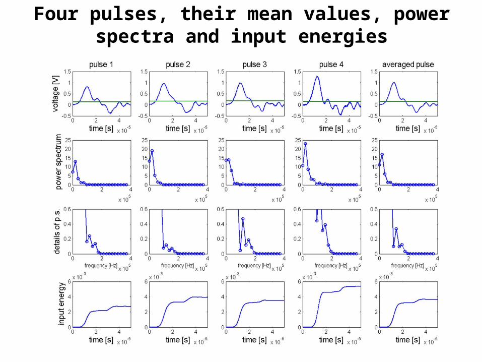
Four pulses, their mean values, power spectra and input energies

Mean value, c0 value, norm and square root of the input energy for different pulses

Terms and statistical tools for

quality assessment of close solutions

• Standard deviation (směrodatná odchylka) of a sample vector (also called series of measurements, signal, list of samples, variables) having n elements is a scalar quantity defined by

• Variance (rozptyl) is the square of the standard deviation.

2

1

1

2

1

1

n

ii xx

ny

n

iixn

x1

1

Covariance

• is the measure of how much two variables vary together (as distinct from variance, which measures how much a single variable varies).

• The algorithm for covariance is

[n,p] = size(X);X = X – ones(n,1)*mean(X);C = X’*X/(n-1);

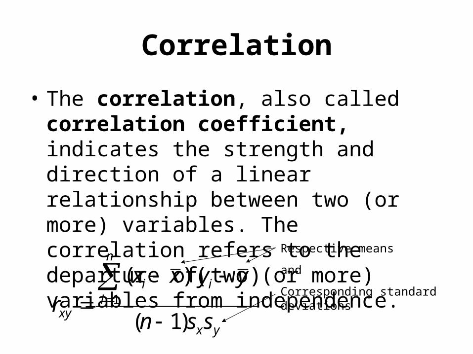
http://en.wikipedia.org/wiki/Variance

Correlation

• The correlation, also called correlation coefficient, indicates the strength and direction of a linear relationship between two (or more) variables. The correlation refers to the departure of two (or more) variables from independence.

yx

n

iii

xy ssn

yyxxr

)1(

))((1

Respective means

and

Corresponding standard deviations

Geometric interpretation of correlation

• The correlation coefficient can also be viewed as the cosine of the angle between the two vectors of samples drawn from the two random variables.

yx

yxuncenteredcos

http://en.wikipedia.org/wiki/Cosine

http://en.wikipedia.org/wiki/Angle

http://en.wikipedia.org/wiki/Vector_%28spatial%29

Validity assessments, Axisymmetric and 3D elements

0 500 1000 1500-1

-0.5

0

0.5

1

1.5

2

2.5x 10

-6

steps

rad

ial d

isp

lac

em

en

ts, l

oc

ati

on

1, l

ay

er

1, n

od

e 1

[m]

Axisym vs. 3D elements, medium striker, CD

axi3D

0 500 1000 15000

1

2

3

4

5

6x 10

-5

steps

ax

ial d

isp

lac

em

en

ts, l

oc

ati

on

1, l

ay

er

1, n

od

e 1

[m

]

Axisym vs. 3D elements, medium striker, CD

axi3D

Quantitative measure of agreement quality

The agreement of solutions obtained by a different element types is excellent – for a given loading and the employed time and space discretizations, there is almost no ‘measurable’ difference.

One way to measure the difference between two solutions, having the form of a vector in n-dimensional space (n is the number of time steps in this case), is to compute the angle between them. In our case the quality of agreement could be quantified by

320209978474978.0cos

yx

yx

This value is called the uncentered correlation coefficient.

Assessment of solutions obtained by means of NM and CD operators

and for different time and space discretizations

0 0.5 1 1.5 2 2.5 3 3.5 4 4.5

x 10-5

-2

-1

0

1

2

x 10-6 four meshes, original data, axisym, NM

rad

ial d

isp

lace

me

nts

, co

rne

r n

od

e, l

ocC

time

0 0.5 1 1.5 2 2.5 3 3.5 4 4.5

x 10-5

-2

-1

0

1

2

x 10-6 four meshes, original data, axisym, CD

time

rad

ial d

isp

lace

me

nts

, co

rne

r n

od

e, l

ocC

m1m2m3m4

m1m2m3m4

Measure of sameness by correlation

2 3 40

0.005

0.01

0.015

0.02

0.025

m2 to m4, <j> index

relative directional error of m to m<j> data, NM

2 3 40

0.005

0.01

0.015

0.02

0.025

m2 to m4, <j> index

relative directional error of m to m<j> data, CD

m1, indexm2, indexm3, index

m1, indexm2, indexm3, index

Measure of sameness by variance and covariance

1 2 3 41.46

1.48

1.5

1.52

1.54

1.56

1.58

1.6x 10

-12 variance and covariance for m1 to m4

meshes m1 to m4

variance for NM

variance for CDcovariance NM. vs. CD

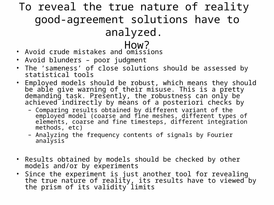
To reveal the true nature of reality good-agreement solutions have to analyzed.

How?• Avoid crude mistakes and omissions • Avoid blunders – poor judgment• The ‘sameness’ of close solutions should be assessed by statistical

tools• Employed models should be robust, which means they should be

able give warning of their misuse. This is a pretty demanding task. Presently, the robustness can only be achieved indirectly by means of a posteriori checks by– Comparing results obtained by different variant of the employed model

(coarse and fine meshes, different types of elements, coarse and fine timesteps, different integration methods, etc)

– Analyzing the frequency contents of signals by Fourier analysis

• Results obtained by models should be checked by other models and/or by experiments

• Since the experiment is just another tool for revealing the true nature of reality, its results have to viewed by the prism of its validity limits

Conclusions

When trying to ascertain the reliability of modelling approaches and the extent of their validity one has to realize that the models as a rule do not have self-correction features. That’s why we have to let the models to check themselves, be checked by independent models and let the systematic doubt be our everyday companion.

Leftovers

Solution of impact tasks, assessment of result reliability M. Okrouhlík Institute of...

Documents

Transcript of Solution of impact tasks, assessment of result reliability M. Okrouhlík Institute of...