


Solution Manual for Foundations of Operations …...Solution Manual for Foundations of Operations...
73
Solution Manual for Foundations of Operations Management 3th Canadian Edition by Ritzman Chapter 2 Supply-Chain Management PROBLEMS 1. Buzzrite Company a. Current Year’s average aggregate value = $48,000,000/6 = $8,000,000 Next year ’s average aggregate inventory value = ($48,000,000 × 1.25)/6 = $10,000,000 Increase in the average aggregate inventory value = ($10,000,000 – 8,000,000) = $2,000,000 b. Number of turns to support next year ’s sales with no increase in inventory value = (1.25)(6) = 7.5 turns. Thus, the change in inventory turnover = new – old = 1.5 inventory turns, or 25% higher inventory turns. 2. Precision Enterprises. Average aggregate inventory value = Raw materials + WIP + Finished goods = $3,129,500 + $6,237,000 + $2,686,500 = $12,053,000 a. Sales per week = Cost of goods sold/52 weeks per year = $32,500,000/52 = $625,000 Weeks of supply = Average aggregate inventory value/
Transcript of Solution Manual for Foundations of Operations …...Solution Manual for Foundations of Operations...

Solution Manual for Foundations of Operations Management 3th
Canadian Edition by Ritzman
Chapter
2 Supply-Chain Management
PROBLEMS 1. Buzzrite Company
a. Current Year’s average aggregate value = $48,000,000/6 = $8,000,000 Next year’s
average aggregate inventory value = ($48,000,000 × 1.25)/6 = $10,000,000
Increase in the average aggregate inventory value
= ($10,000,000 – 8,000,000) = $2,000,000
b. Number of turns to support next year’s sales with no increase in inventory value = (1.25)(6) = 7.5 turns.
Thus, the change in inventory turnover = new – old = 1.5 inventory turns, or 25% higher inventory turns.
2. Precision Enterprises. Average aggregate inventory value = Raw materials + WIP + Finished goods
= $3,129,500 + $6,237,000 + $2,686,500
= $12,053,000
a. Sales per week
= Cost of goods sold/52 weeks per year = $32,500,000/52
= $625,000
Weeks of supply
= Average aggregate inventory value/

Weekly sales = $12,053,000/$625,000
= 19.28 wk
b. Inventory turnover
= (Annual sales)/(Average aggregate
inventory value)
= $32,500,000/$12,053,000
= 2.6964 turns/year
14

CHAPTER TWO Supply Chain
Management
3. Sterling Inc.
a.
Average
Part Number Inventory (units) Value ($/unit) Total Value ($)
RM-1 20,000 1.00 20,000
RM-2 5,000 5.00 25,000 RM-3 3,000 6.00 18,000
RM-4 1,000 8.00 8,000
WIP-1 6,000 10.00 60,000
WIP-2 8,000 12.00 96,000
FG-1 1,000 65.00 65,000
FG-2 500 88.00 44,000
44,500 336,000
Average aggregate inventory value: $336,000
b. Average weekly sales at cost = $6,500,000/52
= $125,000
Weeks of supply = $336,000/$125,000
= 2.688 weeks.
c. Inventory turnover = Annual sales (at cost) /Average
aggregate inventory value
= $6,500,000/$336,000
= 19.34 turns.
4. One product line Inventory turnover = (Annual sales at cost)/(Average
aggregate inventory value) 10.0 = $985,000/Average aggregate
inventory value
Average aggregate inventory value = $985,000/10 = $98,500
5. A retailer
a.
Sales per week = Cost of goods sold/52 weeks per year = $3,500,000/52
= $67,308
Weeks of supply = Average aggregate inventory value / Weekly sales (at cost)
= $1,200,000/$67,308 = 17.8 wk
15

CHAPTER TWO Supply Chain Management
b. Inventory turnover = (Annual sales at cost) /
(Average aggregate inventory value) = $3,500,000/$1,200,000
= 2.9 turns/year
16

CHAPTER TWO Supply Chain
Management
DISCUSSION QUESTIONS
1. Humanitarian supply chains aimed at disaster relief have all of the characteristics of a responsive supply chain
design. Essentially the strategy is assemble-to-order (many standardized items taken to specific locations). Lead
times must be short. Fast delivery, volume flexibility, and of, course high levels of quality are necessary.
Forward placement of inventories (i.e., critical supplies of water, blankets, food, chainsaws) can reduce lead
times. The challenge is that often a humanitarian supply chain must be created after the disaster has struck,
creating immense challenges, such as those that followed the massive ice storm in Quebec in 1998. That is why
trucking and delivery firms with operations in these areas can be very helpful because their supply chains are
already in place. The management of a humanitarian supply chain must have the ability to integrate the help
(and supply chains) of many organizations.
2. A number of possible benefits can come from the change from plastic foam clamshells to paper wrappings.
First, by undergoing the changes needed to employ the new wrappings, the company may learn to become more
efficient in how it uses packaging. Second, this action is very visible to customers, which can provide a public
relations benefit and increase sales. Third, depending on the formulation of the paper wrapper and the
development of an effective recycling system, the environmental impact might be reduced. Typical plastic foam
is not bio-degradable and difficult to recycle. Fourth, disposal costs costs might be reduced, although these
would be offset to some extent by recycling expenses. However, several potential downsides need to be considered. First, the severance of long-time suppliers
may have a negative impact on the remaining suppliers if they feel the company will cancel contracts as public sentiment shifts on an environmental issue. The operations strategy in the past leveraged supplier loyalty and
innovation; this incident may appear to contradict the understanding the suppliers had that the company will stand by them through difficult times. Second, there will be new packaging to design and suppliers to
coordinate. Such changes might require different communication practices and additional management
oversight, at least in the near future. Moreover, the performance of the paper packaging might be worse (e.g., the food cools faster). Third, the operations strategy, which has been successful, banked on consistency in
operations from restaurant to restaurant. With the change in wrappings comes change in waste disposal and
recycling operations, which are likely to vary from city to city, or province to province. The downsides can be overcome; however, it is critical that such a decisions has long-term
consequences for the supply chain.
3. Wal-Mart’s approach is to generate a competitive situation between suppliers and to drive down prices. One of
the major competitive priorities in Wal-Mart’s business is low cost, thereby keeping retail prices to a minimum. Wal-Mart is dealing with standardized goods in high volumes, and consequently uses an efficient supply chain.
The Limited deals with fashion goods that have shorter life cycles. Therefore, the Limited needs a more flexible supply chain and also more control over the supply channels. Mast Industries provides the capability to
produce fashion goods quickly.
17

CHAPTER TWO Supply Chain Management
4. Many of the key suppliers for Autoshare are service-based, including information technology that track cars,
property management firms that own the parking lots, auto mechanics for preventive maintenance and repairs,
and suppliers of fuel. Of course, automobile manufacturers are critical suppliers to provide new vehicles to
replace older cars, ideally with a more fuel efficient design. In contrast, Bombardier has a network of very
sophisticated suppliers that manufacture parts and subsystems, in addition to its own plant network. Autoshare is working with partners to expand the number of locations to expand customer service and the
value of membership. Thus, its primary focus is on downstream linkages with property owners to increase
access. In parallel, AutoShare’s service suppliers also need to expand their ability to serve a growing number of
locations. In contrast, Bombardier is working to develop upstream linkages with its suppliers—to the point
where much the of the technology development work is their responsibility. As an aircraft designer and
integrator, web-based technologies can improve collaboration during design, the speed of information
exchange, and scheduling once production begins. This is particularly important as the extent of design and
manufacturing work by suppliers continues to expand. AutoShare is heavily using the web to interact with customers and track usage. In addition, web-based data
exchange also might be used to schedule maintenance and other background services. Similar to AutoShare,
Bombardier could include customers in the web-based system, once a new aircraft is launched into production.
Here, customized options or changes could be readily captured into scheduling, and customers could monitor
their orders as they move through the system. The web may also facilitate the more timely collection of
operating performance data for its aircraft in service. Thus, the web can offer a new option for Bombardier to
develop closer relationships with its customers.
18

CHAPTER TWO Supply Chain
Management
CASE: WOLF MOTORS *
A. Synopsis Wolf Motors has just expanded its network of auto dealerships to include its first auto supermarket where three
different makes of cars are sold at the same facility. John Wolf, the president and owner of the dealership, has
identified three factors that have contributed to the success of the dealerships: volume, ―one price-lowest price‖
concept of pricing, and after-the-sale service to the cars sold. Focusing on the service aspect, three components
are critical to providing quality after-the-sale service: well-trained technicians, the latest equipment
technologies, and an adequate supply of service parts and materials. Presently each dealership is responsible for
ordering and managing its inventory of parts and service materials. The recent growth has brought with it both
space and financial resource constraints. John is now wondering what, if anything, can be done with respect to
the purchasing of service parts and materials that would help address some of these concerns.
B. Purpose This case provides students with the opportunity to investigate the purchasing function of an organization in the service sector. Students begin to see that the effective management of materials is not only essential in manufacturing environments but is also critical in supporting the delivery of quality services.
Students are confronted by a number of issues as they are asked to recommend a suitable structure for the purchasing function. Included among them are the following: 1. Given the growth in the number of dealerships in the network, should the purchasing function be
centralized to take advantage of certain economics of scale, or should it remain decentralized in each
separate dealership?
2. Given the different categories of service parts that are purchased, supplier management issues are raised.
Some parts may be more appropriately purchased through single-source contracting, whereas others may be
competitively bid on by multiple suppliers. Bid awards don’t necessarily have to be awarded on the basis of
low cost alone. Also some items may be grouped and purchased from the same supplier using blanket
orders.
3. Limited space for inventory storage and limited investment dollars complicate the issues. Fast, reliable
service in repairing and servicing cars is a key factor in the success of the dealership, but space and dollars
limit service part availability to some extent.
4. Finally, students have the opportunity to bring into play basic inventory management concepts such as an
ABC analysis to help determine appropriate levels of inventory investment and inventory stocking policies.
This case can also be used as a lead-in to Chapter 10, Inventory Management.
* This case was prepared by Dr. Brooke Saladin, Wake Forest University, as a basis for classroom discussion.
19

CHAPTER TWO Supply Chain Management
C. Analysis The analysis of this case can be accomplished in three logical steps. Students should first address the issue of restructuring the purchasing function. Then the inherent policies and procedures to carry out the purchasing
processes can be addressed, followed by an analysis of specific inventory management issues that help lead into Chapter 10, Inventory Management.
Major factors to consider in addressing these steps include: Presently each individual dealership handles its own purchase and management of service parts
and materials. The new dealership is an auto supermarket with three different makes of cars sold at the same location. The
purchase of this dealership has led to a tightening of financial resources. Having three different makes of
cars to service has also created a space constraint in stocking service parts. Wolf Motors is trying to reduce the total operating costs in order to compete effectively in a very price
competitive market with its ―one price-lowest price‖ strategy, while at the same time it needs to maintain a
high level of service. High service levels have traditionally been linked to high levels of inventory of spare
parts.
There is a need to maintain timely delivery of service parts due to the limited space available. There are various categories of parts and materials. One key distinction is that some parts are available only
from the auto manufacturer or its certified dealer/wholesaler. Other parts and materials (i.e., oil, lubricants,
fan belts, and so on) are more generic and can be purchased from a number of sources, including local
vendors. Parts are not only used to service and repair cars but are also sold over-the-counter to the do-it-yourself
mechanic or other repair garages. Therefore, the overall levels of demand and supporting inventory must be
coordinated among service needs, sales, and special promotions such as free brake inspections or discounts
on oil changes and air-conditioner service. Weather also plays a role in the demand for parts: extreme cold
affects the electrical/ignition systems, heat affects the air-conditioning, and rain affects the wipers.
1. Structural Issues: Students should first address the structural issues that face Wolf Motors pertaining to the purchase of parts and materials. These issues include two categories of decisions: (1) centralized
purchasing versus continuing a decentralized model of letting each dealership purchase and manage its own
inventories and (2) the responsibility relationships purchasing should maintain with inventory management
and control, to include the distribution of parts for service and over-the-counter sales. Although there is some advantage to be gained by maintaining a decentralized, local purchasing
function, it appears that Wolf Motors has grown to the point where a more formal central purchasing
function is warranted. Wolf’s size should give it some economy of scale leverage to help maintain low costs and timely deliveries.
Within the purchasing function, personnel could be assigned specific responsibilities or vendors such as:
Specific auto manufacturers or their certified distributors Wholesale distributors of generic parts such as alternators, carburetors, or brake pads
Wholesale distributors of consumable materials such as oils, lubricants, or filters
20

CHAPTER TWO Supply Chain
Management
The second structural issue pertains to the level of integration that needs to be structured and
maintained between purchasing, inventory stocking and control, and parts distribution. Should these be
separate functions that ―hand off‖ the responsibility for materials as they flow through the system, or
should an integrated supply chain be implemented? The issue is one of being able to balance the purchasing
costs, inventory carrying costs, distribution/logistics costs, and target service levels.
2. Policies and Procedures: After the structural issues have been discussed, students should consider
alternative purchasing options that are available for procuring parts. Given that the parts and materials
being purchased differ quite a bit with respect to availability, usage, costs, and delivery lead time, the
policies and procedures used to order various parts may be different. Alternative policies that may be used
include: Competitive bidding
Single-source contracting
Blanket orders Open-
ended orders
Of course, these approaches are not mutually exclusive and may be combined for certain categories of
parts. Students should discuss how each of these alternatives may be used for different groups of parts and
materials. Going out for competitive bids would be most appropriate for ―commodity‖ type items that are
readily available from a number of vendors. Given that other aspects of the service, such as reliability and
dependability, are comparable, then a competitive bid will help reduce purchase costs. Where the quality of
the parts and/or service provided differs, then a single-source contract may be warranted. This should lead
to a partnership arrangement that is beneficial to both parties. Blanket orders are used when a number of parts are to be purchased from a single supplier. Blanket
orders help reduce the overall ordering and distribution costs by grouping items under a single order. This may be an appropriate procedure for purchasing oils and lubricants from a local supplier or for ordering ―factory certified‖ parts from a manufacturer or its designated distributor.
Open-ended orders provide flexibility in allowing items to be added or deleted from an order or for the
time period of the order to be extended, such as in a blanket order of oil. Through this discussion students
will begin to see that all items should not be ordered by the same procedure. Factors such as the item’s
availability, relative importance, usage levels, and costs will have a significant impact on the way the item
should be procured. This has implications also in determining how the purchasing function’s performance
should be measured and evaluated. Just getting the lowest price is no longer good enough. Other measures
of performance, such as product quality, reliable on-time delivery, and ordering flexibility with respect to
the size and timing of the order, may be more important than price. This is an important lesson the students
should understand.
3. Inventory Management Issues: The financial resource and space constraint issues brought out in the case
provide the opportunity to discuss the close relationship and necessary integration that purchasing must
have with inventory management. Suggested inventory management policies that can be discussed include
the three important factors in making inventory stocking-level decisions. These include costs, delivery lead
time, and space
21

CHAPTER TWO Supply Chain Management
required/available. Students should see that each of these factors can be used to prioritize the different
parts and materials to be inventoried. You can discuss the different costs incurred in ordering and carrying inventory to set students up
for the trade-offs to be discussed in the Inventory Management chapter. You can bring out the issue of total investment in inventory over time to open the door for a
discussion of the ABC analysis in the Inventory Management chapter. There is the issue of where to stock different parts in the storeroom or warehouse. Frequently used
material should be stored in easily accessed locations, and a random location system will minimize
space requirements. You could also introduce how inventories can be categorized, such as building anticipation stocks for
promotions and seasonal use. Finally, perhaps implementing an effective EDI link between locations and
suppliers would reduce delivery lead time. The amount of time and depth of analysis pertaining to the discussion of inventory management issues
will depend on how you wish to lead into the chapter on inventory management. You should at least make sure the students see the necessary integration between purchasing and inventory management policies.
D. Recommendations How the case is used will determine the level of detail you should expect with respect to any recommendations students may make. When used as an in-class exercise without any prior preparation by the students, the focus
of the case should be on discussing the issues and recognizing the trade-offs that need to be made in the decisions. If given more time to read and analyze the case, typical recommendations to expect include: 1. Some form of centralization of the purchasing function
2. Development of partnership agreements for ―key‖ parts that perhaps may lead to single sourcing
3. The use of blanket orders to reduce ordering costs and to limit the number of suppliers
4. Open-ended ordering agreements, especially in the ―commodity‖ type materials that can be sourced
locally to reduce lead times and minimize inventory investment
5. Perhaps the establishment of a central warehouse facility to reduce overall space requirements
while maintaining parts availability in a timely manner
6. Conducting an analysis of inventory cost trade-offs to minimize total costs of inventory policies
E. Teaching Suggestions This case can be used as either an in-class ―cold-call‖ exercise or an overnight reading and analysis exercise. In either case the class discussion flows well when the instructor follows the order of the discussion questions at the end of the case. The level of detail necessary to make this a good decision case is not present. The case was designed to act as a vehicle to introduce the issues that pertain to purchasing and to show students that the issues
are similar
22

CHAPTER TWO Supply Chain
Management
in both services and manufacturing. Therefore, it is best to begin the discussion by first focusing on how the
purchasing function should be organized. Then focus the students on specific policies and procedures that Wolf
may implement for different categories of parts. Finally, if time permits, you can begin to introduce some
inventory management issues and show how the inventory function interacts with purchasing.
23
CHAPTER TWO Supply Chain Management
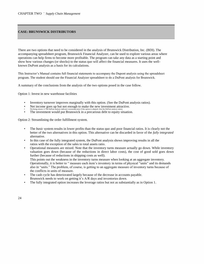
CASE: BRUNSWICK DISTRIBUTORS
There are two options that need to be considered in the analysis of Brunswick Distribution, Inc. (BDI). The
accompanying spreadsheet program, Brunswick Financial Analyzer, can be used to explore various areas where
operations can help firms to become more profitable. The program can take any data as a starting point and
show how various changes (or shocks) to the status quo will affect the financial measures. It uses the well-
known DuPont analysis as a basis for its calculations.
This Instructor’s Manual contains full financial statements to accompany the Dupont analysis using the spreadsheet
program. The student should use the Financial Analyzer spreadsheet to do a DuPont analysis for Brunswick.
A summary of the conclusions from the analysis of the two options posed in the case follow.
Option 1: Invest in new warehouse facilities
• Inventory turnover improves marginally with this option. (See the DuPont analysis ratios). • Net income goes up but not enough to make the new investment attractive. • Declining returns ⇒ The DuPont analysis indicates worsening ratios if this option is adopted. (See the DuPont analysis ratios).
• The investment would put Brunswick in a precarious debt to equity situation.
Option 2: Streamlining the order fulfillment system.
• The basic system results in lower profits than the status quo and poor financial ratios. It is clearly not the
better of the two alternatives in this option. This alternative can be discarded in favor of the fully integrated
alternative. • In this case of the fully integrated system, the DuPont analysis shows improving results in all the
ratios with the exception of the sales to total assets ratio. • Operational measures are mixed. Note that the inventory turns measure actually go down. While inventory
valuation goes down (because of the reductions in direct labor costs), the cost of good sold goes down further (because of reductions in shipping costs as well). This points out the weakness in the inventory turns measure when looking at an aggregate inventory. Operationally, it is better to ― measure each item’s inventory in terms of physical ―units‖ and its demands
also in ―units.‖ The problem, of course, is getting to an aggregate measure of inventory turns because of
the conflicts in units of measure. • The cash cycle has deteriorated largely because of the decrease in accounts payable.
Brunswick needs to work on getting it’s A/R days and inventories down. • The fully integrated option increases the leverage ratios but not as substantially as in Option 1.
24

CHAPTER TWO Supply Chain
Management
• Another reason why Option 2 is the better than Option 1 is its impact on the stock market
performance measures.
While Option 2 – fully integrated system – dominates Option 1, it does not improve the inventory problems at
Brunswick. ―Inventory days‖ goes up and ―inventory turns‖ go down. Brunswick may decide to take Option 2 for
other reasons. This option may improve customer service and drive increases in customer demands in the future.
The analysis of these two options shows the tradeoff in attempting to build market share (Option 1) and becoming
more efficient (Option 2). It should be pointed out to the students that the Dupont analysis is a short-term analysis.
It is debatable which of the two options may have more long-term benefits.
Educational objectives
• To critically examine the inter-related activities of marketing, finance and operations. • To study how seemingly small changes in various aspects of the business affect return on equity
and financial measures. • To emphasize that operational changes that affect the cost of goods sold (such as direct materials costs or labor
costs) can have an effect on the firm’s inventory measures because of the way inventory is valued, even if the actual stock of inventory remains unchanged.
DISCUSSION Option 1
Income statement
• This option increases annual revenue by $3.6 million.
• This option would increase costs by a total of $1,717,000, split up between shipping ($955 thousand), direct material ($358 thousand), and direct labor cost ($404 thousand).
• Annual depreciation works out to be $500,000, which is computed as straight-line depreciation of
the $10 million investment for 20 years. ($10 million/20)
• Annual interest is computed at the rate of 11%. (11%*$12 million = $1,320,000)
Balance sheet
• $1.5 million in accounts receivable.
• $10 million investment in plant and equipment.
• $2 million in property.
• The Financial Analyzer assumes that the new level of inventory investment is equal to the old level,
plus direct changes (plus or minus) in the shock column, plus one-half the total
25

CHAPTER TWO Supply Chain Management
of the changes to the direct materials on the Income Statement (plus or minus) and the changes to the
direct labor on the Income Statement (plus or minus). The Financial Analyzer will automatically do this
computation, given the inputs on the Income Statement and the direct inventory shock. Here we have
assumed that direct materials changes and the labor changes take place gradually over the course of the
year so that the average level is one half of the total.
• On the liability side accounts payable is increased by the amount of the interest from the new loan, adjusted
downward for savings in materials and labor, and adjusted for any net changes in taxes. Once the annual
interest is entered in the ―shock‖ column, the Financial Analyzer does the computation for you.
• The entire $12 million is assumed to be a long-term loan agreement.
See the complete spreadsheet analysis for Option 1.
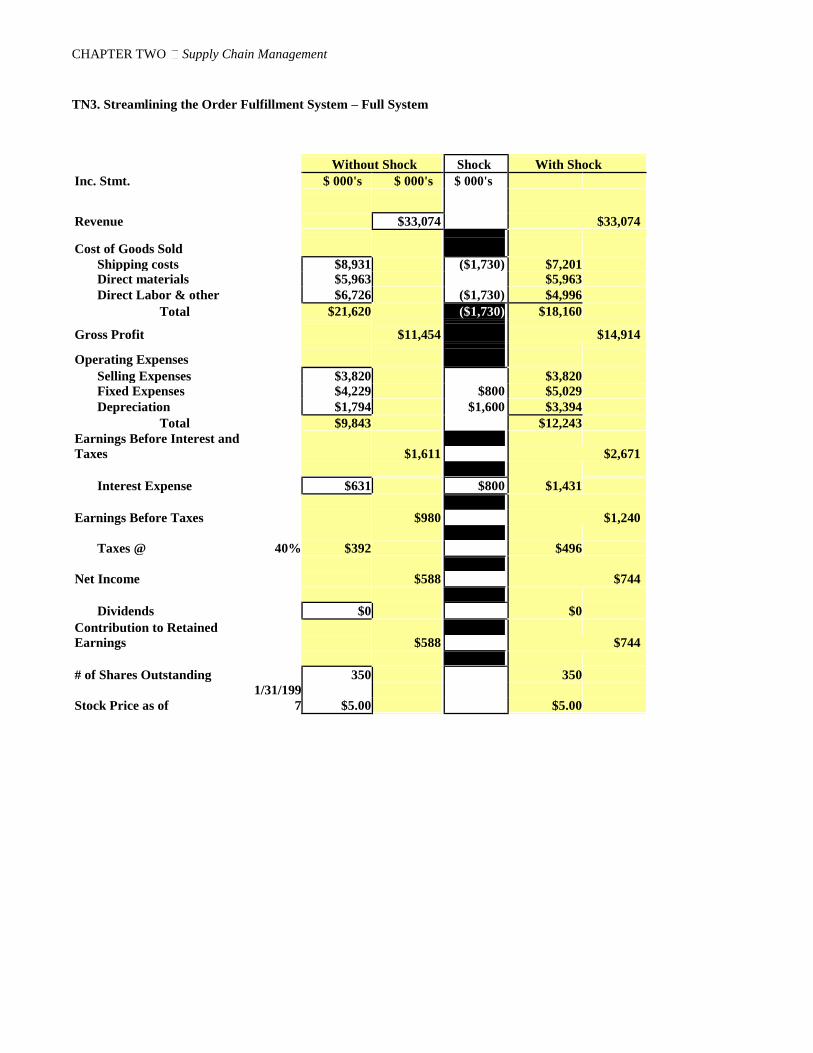
Option 2
This option would contribute 16% in direct cost savings for the fully integrated system which is computed as 16%
* Cost of sales (16%*$21,620,000). This works out to be $3,460,000 in annual savings split up equally for direct
material and direct labor cost – ($1,730,000).
Income Statement
• Annual depreciation works out to be $1,600,000, which is computed as straight-line depreciation
of the $8 million investment for five years. ($8M/5)
• Annual interest is computed at the rate of 10%. 10%*$8 million = $800,000.
Balance Sheet
• $8 million investment in plant and equipment.
• On the liability side, accounts payable is computed as being made up of direct material costs net
of savings and the additional amount payable on the higher taxes resulting from the savings.
• The entire $8 million is assumed to be a long-term loan agreement.
See the complete spreadsheet analysis for the two alternatives of Option 2.
26

CHAPTER TWO Supply Chain
Management
Other Issues to Discuss
One of the biggest issues facing BDI is the predictability of sales. Since orders do not come in from retailers in a
timely fashion, considerable emphasis is placed on forecasting sales for manufacturers. This forecasting is largely
historical and therefore does not reflect the changes that have occurred over the past two years. In order to better
determine levels of safety stock, a better integration of the supply chain is required. Getting the end customer
involved by showcasing the product in a kitchen-like setting and acquiring forward-looking information from the
end user might help Brunswick in determining demand. Perhaps a better approach, however, is to implement
vendor managed inventory programs with retailers and using their forecasts of sales in various product lines. This
could somewhat alleviate the delayed ordering from the retailer and allow more accurate 60/90/120 ordering to the
manufacturer.
With the additional business, and the extra product lines, BDI has acquired some deadweight. The
company already supplies the majority of high-end appliances and the new lines have cut in to the profit margins
that the company has historically observed. Other financial concerns, such as the poor cash cycle, can be looked at
in one of two ways: either bring accounts receivable and accounts payables closer in line by delaying payables
whenever possible and placing tighter controls on receivables, or, increase liquidity by obtaining a larger
operating loan.
27

CHAPTER TWO Supply Chain Management
TN1. Invest in New Warehouse Facilities
Without Shock Shock With Shock
Inc. Stmt. $ 000's $ 000's $ 000's
Revenue
$3,600 $36,674 $33,074
Cost of Goods Sold Shipping costs $8,931 $955 $9,886
Direct materials $5,963 $358 $6,321
Direct Labor & other $6,726 $404 $7,130
Total $21,620 $762 $23,337
Gross Profit
$11,454
$13,337
Operating Expenses
Selling Expenses $3,820 $3,820
Fixed Expenses $4,229 $4,229
Depreciation $1,794 $500 $2,294
Total $9,843 $10,343
Earnings Before Interest and
Taxes $1,611 $2,994
Interest Expense
$1,951
$631 $1,320
Earnings Before Taxes
$980
$1,043
Taxes @ 40% $392
$417
Net Income
$588
$626
Dividends
$0
$0
Contribution to Retained
Earnings $588 $626
# of Shares Outstanding
350
1/31/199
350
Stock Price as of 7 $5.00 $5.00

CHAPTER TWO Supply Chain
Management
TN1 (continued)
Balance Sheet Ass
Without
With
Liabil
Without
With
ets Shock Shock ities Shock Shock
Shoc Shoc
k k
Current Assets Current Liabilities Accounts $1,28 $1,32 $3,38
Payable 2 0 9
Short-term
Liabilities $1,09
$0 $6,7 $7,17 $1,09
Inventory 89 0 Notes Payable 9 9 Total
Inventor $6,78 Short-term $4,15 $4,15
y 9 $7,170 Debt 9 9 Total $6,54
STL 0 8647.2 $3,2 $3,22
Cash 23 3
Accounts $5,6 $1,50 $7,10 Long-term
Receivable 03 0 3 Liabilities Other Current $1,3 $1,38 Long-term $7,52 $12,0 $19,5
Assets 81 1 Loans 3 00 23 $16,9
Total CA 96 $18,877 Bonds $0
Other
Liabilities $0
Total $7,52
LTL 3 $19,523
Long-term Assets $2,00
Property
$3,1 $5,17 Total Debt
$14,0 $28,1
79 0 9 63 70
Plant and $8,9 $10,0 $18,9 Equipment, net 95 00 95
Long-term $1,0 $1,00 $1,75 $1,75
Investments 00 0 Equity 0 0 $13,1
Total LTA 74 $25,174 Common Stock $0
Paid-in-excess $428 $428 Total Assets
$30,1 $44,0 $13,9
$13,7
70 51
Retained Earnings 29 03 Total $16,1 $15,8
Equity 07 81
Total Debt & Equity $30,1 $44,0
70 51

29
CHAPTER TWO Supply Chain Management
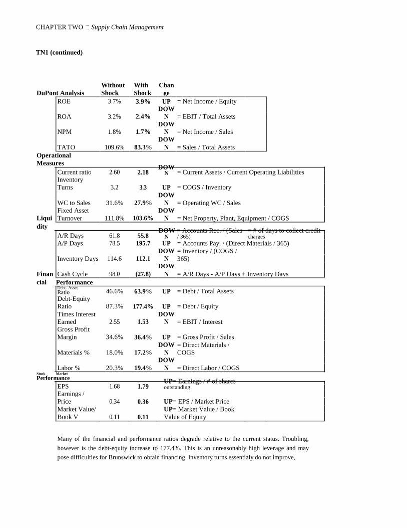
TN1 (continued)
Without With Chan
DuPont Analysis Shock Shock ge
ROE 3.7% 3.9% UP = Net Income / Equity DOW
ROA 3.2% 2.4% N = EBIT / Total Assets
DOW
NPM 1.8% 1.7% N = Net Income / Sales
DOW
TATO 109.6% 83.3% N = Sales / Total Assets
Operational
Measures DOW
Current ratio 2.60 2.18 = Current Assets / Current Operating Liabilities
N
Inventory
Turns 3.2 3.3 UP = COGS / Inventory
DOW
WC to Sales 31.6% 27.9% N = Operating WC / Sales
Fixed Asset DOW
Liqui Turnover 111.8% 103.6% N = Net Property, Plant, Equipment / COGS
dity DOW = Accounts Rec. / (Sales = # of days to collect credit
A/R Days 61.8 55.8
N / 365) charges
A/P Days 78.5 195.7 UP = Accounts Pay. / (Direct Materials / 365)
DOW = Inventory / (COGS /
Inventory Days 114.6 112.1 N 365)
DOW
Finan Cash Cycle 98.0 (27.8) N = A/R Days - A/P Days + Inventory Days
cial Performance Debt- Asset
46.6% 63.9% UP = Debt / Total Assets
Ratio
Debt-Equity
Ratio 87.3% 177.4% UP = Debt / Equity
Times Interest DOW
Earned 2.55 1.53 N = EBIT / Interest
Gross Profit
Margin 34.6% 36.4% UP = Gross Profit / Sales
DOW = Direct Materials /
Materials % 18.0% 17.2% N COGS
DOW
Labor % 20.3% 19.4% N = Direct Labor / COGS Stock Market
Performance UP= Earnings / # of shares
EPS 1.68 1.79
outstanding
Earnings /
Price 0.34 0.36 UP= EPS / Market Price
Market Value/ UP= Market Value / Book
Book V 0.11 0.11 Value of Equity
Many of the financial and performance ratios degrade relative to the current status. Troubling,
however is the debt-equity increase to 177.4%. This is an unreasonably high leverage and may
pose difficulties for Brunswick to obtain financing. Inventory turns essentialy do not improve,

CHAPTER TWO Supply Chain
Management
TN2. Streamlining the Order Fulfillment System – Basic
Without Shock Shock With Shock
Inc. Stmt. $ 000's $ 000's $ 000's
Revenue
$33,074 $33,074
Cost of Goods Sold Shipping costs $8,931 ($1,081) $7,850
Direct materials $5,963 $5,963
Direct Labor & other $6,726 ($1,081) $5,645
Total $21,620 ($1,081) $19,458
Gross Profit $11,454 $13,616
Operating Expenses
Selling Expenses $3,820 $3,820
Fixed Expenses $4,229 $800 $5,029
Depreciation $1,794 $1,160 $2,954
Total $9,843 $11,803
Earnings Before Interest and
Taxes $1,611 $1,813
Interest Expense
$1,161
$631 $530
Earnings Before Taxes
$980
$652
Taxes @ 40% $392
$261
Net Income
$588
$391
Dividends
$0
$0
Contribution to Retained
Earnings $588 $391
# of Shares Outstanding
350
1/31/199
350
Stock Price as of 7 $5.00 $5.00

31

CHAPTER TWO Supply Chain Management
TN2 (continued)
Balance Sheet Ass Without With Liabil Without With
ets Shock Shock ities Shock Shock
Shoc Shoc
k k
Current Assets Current Liabilities Accounts $1,28
Payable 2 $530 $600
Short-term
Liabilities $1,09
$0 $6,7 $6,24 $1,09
Inventory 89 9 Notes Payable 9 9 Total
Inventor $6,78 Short-term $4,15 $4,15
y 9 $6,249 Debt 9 9 Total $6,54
STL 0 5857.8 $3,2 $3,22
Cash 23 3
Accounts $5,6 $5,60 Long-term
Receivable 03 3 Liabilities Other Current $1,3 $1,38 Long-term $7,52 $5,30 $12,8
Assets 81 1 Loans 3 0 23 $16,9
Total CA 96 $16,456 Bonds $0
Other
Liabilities $0 Total $7,52
LTL 3 $12,823
Long-term Assets
Property $3,1 $3,17
Total Debt $14,0 $18,6
79 9 63 81
Plant and $8,9 $5,30 $14,2 Equipment, net 95 0 95
Long-term $1,0 $1,00 $1,75 $1,75
Investments 00 0 Equity 0 0 $13,1
Total LTA 74 $18,474 Common Stock $0
Paid-in-excess $428 $428
Total Assets $30,1 $34,9
$13,9
$14,0
70 30
Retained Earnings 29 71
Total
$16,1
$16,2
Equity 07 49
Total Debt & Equity $30,1 $34,9
70 30

CHAPTER TWO Supply Chain
Management
TN2 (continued)
Without With Chan
DuPont Analysis Shock Shock ge
ROE 3.7% 2.4% DOW
= Net Income / Equity
N
DOW
ROA 3.2% 1.9% N = EBIT / Total Assets
DOW
NPM 1.8% 1.2% N = Net Income / Sales
DOW
TATO 109.6% 94.7% N = Sales / Total Assets
Operational
Measures
Current ratio 2.60 2.81 UP = Current Assets / Current Operating Liabilities
Inventory DOW
Turns 3.2 3.1 N = COGS / Inventory
WC to Sales 31.6% 32.0% UP = Operating WC / Sales
Fixed Asset
Liqui Turnover 80.8% 89.8% UP = Net Property, Plant, Equipment / COGS
dity
A/R Days 61.8
DOW = Accounts Rec. / (Sales = # of days to collect credit
/ 365) charges
A/P Days 78.5 36.7 N = Accounts Pay. / (Direct Materials / 365) = Inventory / (COGS /
Inventory Days 114.6 117.2 UP 365)
Finan Cash Cycle 98.0 142.3 UP = A/R Days - A/P Days + Inventory Days
cial Performance Debt- Asset
46.6% 53.5% UP = Debt / Total Assets
Ratio
Debt-Equity
Ratio 87.3% 115.0% UP = Debt / Equity
Times Interest DOW
Earned 2.55 1.56 N = EBIT / Interest
Gross Profit
Margin 34.6% 41.2% UP = Gross Profit / Sales
= Direct Materials /
Materials % 18.0% DOW COGS
Labor % 20.3% 17.1% N = Direct Labor / COGS Stock Market
Performance DOWN = Earnings / # of
EPS 1.68 1.12
shares outstanding
Earnings /
Price 0.34 0.22 DOWN = EPS / Market Price
Market Value/ DOWN = Market Value /
Book V 0.11 0.11 Book Value of Equity
The basic level option results in less profit per year and worsening financial ratios. Average inventories increase and inventory turns decrease.

33
CHAPTER TWO Supply Chain Management
TN3. Streamlining the Order Fulfillment System – Full System
Without Shock Shock With Shock
Inc. Stmt. $ 000's $ 000's $ 000's
Revenue
$33,074 $33,074
Cost of Goods Sold Shipping costs $8,931 ($1,730) $7,201
Direct materials $5,963 $5,963
Direct Labor & other $6,726 ($1,730) $4,996
Total $21,620 ($1,730) $18,160
Gross Profit
$11,454
$14,914
Operating Expenses
Selling Expenses $3,820 $3,820
Fixed Expenses $4,229 $800 $5,029
Depreciation $1,794 $1,600 $3,394
Total $9,843 $12,243
Earnings Before Interest and
Taxes $1,611 $2,671
Interest Expense
$1,431
$631 $800
Earnings Before Taxes
$980
$1,240
Taxes @ 40% $392
$496
Net Income
$588
$744
Dividends
$0
$0
Contribution to Retained
Earnings $588 $744
# of Shares Outstanding
350
1/31/199
350
Stock Price as of 7 $5.00 $5.00

CHAPTER TWO Supply Chain
Management
TN3 (continued)
Balance Sheet Ass
Without
With
Liabil
Without
With
ets Shock Shock ities Shock Shock
Shoc Shoc
k k
Current Assets Current Liabilities Accounts $1,28
Payable 2 $800 $456
Short-term
Liabilities $1,09
$0 $6,7 $5,92 $1,09
Inventory 89 4 Notes Payable 9 9 Total
Inventor $6,78 Short-term $4,15 $4,15
y 9 $5,924 Debt 9 9 Total $6,54
STL 0 5714 $3,2 $3,22
Cash 23 3
Accounts $5,6 $5,60 Long-term
Receivable 03 3 Liabilities Other Current $1,3 $1,38 Long-term $7,52 $8,00 $15,5
Assets 81 1 Loans 3 0 23 $16,9
Total CA 96 $16,131 Bonds $0
Other
Liabilities $0
Total $7,52
LTL 3 $15,523
Long-term Assets Property
$3,1 $3,17 Total Debt
$14,0 $21,2
79 9 63 37
Plant and $8,9 $8,00 $16,9 Equipment, net 95 0 95
Long-term $1,0 $1,00 $1,75 $1,75
Investments 00 0 Equity 0 0 $13,1
Total LTA 74 $21,174 Common Stock $0
Paid-in-excess $428 $428 Total Assets
$30,1 $37,3 $13,9
$13,8
70 05
Retained Earnings 29 90 Total $16,1 $16,0
Equity 07 68
Total Debt & Equity $30,1 $37,3
70 05

35

CHAPTER TWO Supply Chain Management
TN3 (continued)
Without With Chan
DuPont Analysis Shock Shock ge
ROE 3.7% 4.6% UP = Net Income / Equity
ROA 3.2% 3.3% UP = EBIT / Total Assets
NPM 1.8% 2.2% UP = Net Income / Sales
DOW
TATO 109.6% 88.7% N = Sales / Total Assets
Operational
Measures
Current ratio 2.60 2.82 UP = Current Assets / Current Operating Liabilities
Inventory DOW
Turns 3.2 3.1 N = COGS / Inventory
DOW
WC to Sales 31.6% 31.5% N = Operating WC / Sales
Fixed Asset
Liqui Turnover 93.3% 111.1% UP = Net Property, Plant, Equipment / COGS
dity = Accounts Rec. / (Sales = # of days to collect credit
A/R Days 61.8
DOW
/ 365) charges
A/P Days 78.5 27.9 N = Accounts Pay. / (Direct Materials / 365)
= Inventory / (COGS /
Inventory Days 114.6 119.1 UP 365)
Finan Cash Cycle 98.0 153.0 UP = A/R Days - A/P Days + Inventory Days
cial Performance Debt- Asset
46.6% 56.9% UP = Debt / Total Assets
Ratio
Debt-Equity
Ratio 87.3% 132.2% UP = Debt / Equity
Times Interest DOW
Earned 2.55 1.87 N = EBIT / Interest
Gross Profit
Margin 34.6% 45.1% UP = Gross Profit / Sales
= Direct Materials /
Materials % 18.0% DOW COGS
Labor % 20.3% 15.1% N = Direct Labor / COGS Stock Market
Performance UP= Earnings / # of shares
EPS 1.68 2.13
outstanding
Earnings /
Price 0.34 0.43 UP= EPS / Market Price
Market Value/ UP= Market Value / Book
Book V 0.11 0.11 Value of Equity
The fully integrated option dominates the basic option as well as Option 1. The financial ratios
are beter, however none of the options addresses the issue of inventory turns. Brunswick may
decide on Option 2: Full Implementation for otjher reasons, primarily customer service that
may pay off in more customers in the future.

CHAPTER TWO Supply Chain
Management
EXPERIENTIAL EXERCISE: SONIC DISTRIBUTORS
A. Synopsis The purpose of this exercise is to provide a situation in which students can observe how supply-chain
management affects the efficiency and effectiveness of a distribution network. It is designed to be quite flexible.
In its simplest form it can be a ―quick hit‖ to give the students an initial exposure to supply chains and thus set
them up for a more productive lecture and discussion of the chapter. Alternatively complexity can be added so
the efficient and the responsive distribution chains can be compared or more freedom can be allowed making it
an analytical simulation to observe and measure the effects of changes to the system. In this last format,
students can configure the supply chain for efficiency or responsiveness (or anywhere in between) and then
operate it while measuring its supply-chain performance. Many lessons can be brought out from a discussion of the results of this exercise. It demonstrates the
complexities of managing an enterprise where there are multiple parties and information requirements involved.
It brings forth the trade-offs that must be made when conflicting goals exist with different costs or benefits. It shows the cost implications of managerial decisions such as establishing safety stock policies and setting
production lot sizes. And, it shows the role of time delay on the overall system performance. The results of this exercise can also lead to further discussions: The distribution of demand for the
distribution centers (and thus for the factory) depends not only on the nature of the demand at the retail stores
but also on the ordering policies of the retailer and the distribution center. This can lead to a discussion of
dependent demand, which sets the stage for the next chapter’s material. As a tie-in to applied statistics, the
smoothing effect of grouping several independent demands, and perhaps, even the central limit theorem can be
teased out of the results. An outline of some of the topics from Chapter 8 that spring from this exercise can be
found at the end of this teaching note.
B. Preparation Materials
Retail and Distributor Purchase Order Forms (one set for each retail store and one set for each of the two
distribution centers). A set is made up of one form for each simulated day the game is to be played. Manufacturing Work Order Sheet (one set for the factory). The set for the factory contains as many forms
as the proposed length of the simulation times the number of distributors it serves. Factory and Distributor Material Delivery Forms (one set for the factory and one set for each distribution
center that the factory supplies). The size of the set for a distributor is the proposed number of days times
the number of retail stores each is to serve.
Inventory Position Worksheets (one for each retail store, each distribution center, and the factory)
37

CHAPTER TWO Supply Chain Management
A random demand generator such as a pair of dice, a deck of playing cards for each team (with all face
cards removed) or slips of paper with the numbers 1 to 10 written on them, random number table, a simple computer program, etc.
Preparation Time Required Instructor: It will take a couple of hours to read through the material and fully understand the procedure that
the students will enact. It is suggested that the instructor personally play several rounds before presenting it in class to the students. The instructor should play the part of all participants (retail stores, distribution centers, and
the factory) to best grasp each student’s role. Although it appears complex at first, the procedure is fairly
simple. Preclass preparation consists of devising the random demand generators, one for each company (team). If
only one type of CD is to be produced (Quick-Hit version), a pair of dice works well (one pair for each retail store is best but a pair can be shared by the stores in a team). If the demonstration is to include all four types of
CD demands, an easy demand generator is a shuffled deck of playing cards with all the face cards and jokers
removed. Inventory position and cost calculation worksheets need to be photocopied, one for each retail outlet,
distributor, and factory. Likewise, sets of Retail Store and Distribution Center Purchase Order Forms, Factory Work Order Forms, and Factory and Distribution Center Material Delivery Forms need to be photocopied. Students: Prereading the exercise is suggested; it reduces the startup time. It should take the students only 15
minutes or so to read and understand the instructions. Indicate to the students how the exercise will be run (the
―Quick Hit‖ version in the text or the ―Efficient versus Responsive Comparison‖ or the ―Analytical Simulation‖ versions in this teaching note). Class Time Required As with any business simulation, there is a trade-off between realism and feasibility. More detail can yield a
more realistic estimate of what true distribution chain costs are. This realism comes at the cost of more effort on
the part of the student to perform the exercise. It also can cause more confusion when trying to explain the
rationale behind each cost and how to account for it when calculating total cost. Therefore, three versions of the
exercise are suggested to allow whatever level of realism the instructor chooses; other configurations are easily
devised, depending on the objectives the instructor. In its simplest form, the ―Quick Hit‖ version can take as little as 45 minutes to run. This has enough detail
for the students to observe the dynamics of a supply chain. The ―Efficient versus Responsive Comparison‖ version takes about 75 minutes. The ―Analytical Simulation‖ version generates the most realistic total costs and
allows the students try several configurations. Therefore, it can take two hours or more plus additional time for postexercise debriefing and discussion. This longer configuration works best for a one-night-per-week class or
if the debriefing and discussion session can take place during the following class. It could also be given as a
multiple session exercise if the goal of the instructor is to cover distribution chain performance in depth. Setting Up This exercise works well when two or more companies are formed. In any case, companies should be
configured with no fewer than two retail outlets drawing from each of the two distributors. Although this is the minimum, more than two retail outlets to each distributor are better because they more clearly demonstrate the
effect of averaging stochastic demand at the distributors. If teams of less than 14 must be formed, first assign
only one person to the
38

CHAPTER TWO Supply Chain
Management
retail stores; next assign only one person to the factory; finally, assign only one to each of the distribution
centers. Play will progress a little more slowly because the students working alone will have more to do (both
undertake the transactions and record them). The following parameters need to be established for each team:
1. Starting conditions:
Initial inventory of each of the four artist’s CDs at the:
Retail stores—the text suggests 15
Distribution centers—the text suggests 25 Factory—the text suggests 100
Outstanding orders (or backorders—if any) for each of the four CDs at the:
Distribution centers—the text suggests none
Factory—the text suggests none
Note: There will be no backorders at the Retail Stores because any stockout results in a lost sale.
2. Operating considerations: Demand patterns—will a quantity of only one artist’s CD be sold at a given retail store each day (i.e., each
retailer will generate only one random number for demand per round—as for the Quick Hit version) or will several artist’s CDs be sold (i.e., each retailer will generate several different random numbers to determine
demand)?
3. Costs Transportation costs and holding costs in the inventory pipeline are expressly ignored in the Quick Hit version for simplicity. Holding cost per unit per day—may be different for each of the stages in the distribution chain.1 The text suggests:
Retail outlets—$1.00/day
Distribution center—$0.50/day Factory—$0.25/day
Ordering/setup cost—may be different for each of the stages in the distribution chain.
The text suggests:
Retail outlets—$20.00/order
Distribution center—$20.00/order Factory setup—$50 per order. For other versions with a capacity limited factory, the setup cost does not recur in subsequent days of production until another order is called for.
Stockout cost (may be different for each stage—will be equivalent to the contribution margin of a lost sale for the retail stores) the text suggests $8.00 for each CD short in a period. Expediting cost (for example, shipping an order by UPS instead of normal freight). The text doesn’t suggest a cost for the Quick Hit version.
1 These holding costs differentials are designed to dissuade students from positioning too much forward inventory
at the retail outlets. See a discussion of other possibilities in the parameter list for the Efficient vs. Responsive version, later on.
39

CHAPTER TWO Supply Chain Management 4. Delays
Ordering delay—time from when a purchase order (PO) is issued until it is received. The text suggests one day. Delivery delay—time required to assemble, pack, and transport an order once the PO is received. The text suggests one day. Production time—time from receiving an order until it is ready for shipment (may be determined by factory production lot sizes). The text suggests one day. If the factory is capacity limited, the delivery delay will be as long as it takes to run the entire order. Partial production runs are not shipped.
5. Lot sizing restrictions—may be EOQ, lot-for-lot, minimum order quantity, or fixed lot size: Retail Store
orders—the text indicates there are none. Distribution Center orders—the text indicates there are none. Factory production lot sizes and capacity. Also, the factory may be able to produce multiple types
simultaneously or be restricted to producing only one type of CD at a time. For the Quick Hit version, the
text suggests a minimum lot size of 20 and an upper limit of 200, which is well above any required
production. For the Quick Hit version, this large capacity eliminates the complexity needing to extend a
production run over several days.
6. Storage capacity restrictions—the text does not mention any for the Quick Hit version.
All of these parameters will be preset by the instructor for the ―Quick Hit‖ and the ―Efficient versus
Responsive Comparison‖ versions. The ―Analytical Simulation‖ version allows students to adjust many of the
operating considerations by making lot sizing and cost/performance trade-off decisions.
C. Conducting the Exercise Break the class into teams and have them sit together so that communication among the team members will be
convenient. They can be seated in an area of the classroom or around a large table. Let them arrange themselves
to establish effective and efficient transmission chains for the required information (POs and material delivery
forms). To include delays in the transmission of POs to suppliers or in the delivery of goods from suppliers,
provide a place where the POs and delivery forms can be placed for the required delay periods. If the team is
seated at a table, 8 ½ × 11 pieces of paper (one for each source and sink pair) can be fastened on the table and
marked as delay stations. If the students are sitting in chairs, an empty chair between the various pairs within
the team can serve as a delay station. Specify the values for the parameters (listed previously) that will be followed for the exercise. Review the
sequence of play. If a deck of cards or slips of paper are used to determine demand, specify that at the end of
each round (day) the cards or slips that were drawn should be returned to the deck and the deck reshuffled. Go over the items that are to be recorded on the worksheets. Start off with a few practice rounds to be sure each
student understands his or her task, how the data are gathered, and how play progresses.
40

CHAPTER TWO Supply Chain
Management
To simplify record keeping, have the students adopt an MRP ―midpoint convention‖ for recording
transactions. This assumes all transactions occur simultaneously in the middle of the day—scheduled receipts
arrive, demand is determined and met, and any shortages occur, all at noon. Inventory recorded in the inventory
position worksheet is the ending inventory after all these transactions occur. Regardless of the version, for each simulated day the sequence of play goes as follows:
Retailer: a. Each retailer receives any shipment due in from their distributor (one day after shipment) and places it into
sales inventory (adds the quantity indicated on any incoming Material Delivery Form from the distributor—after its one-day delay—to the current inventory level on the Retailer’s Inventory Position
Worksheet). Note: for the first day of the exercise no order will be coming in. b. The retailers each determine the day’s retail demand (the quantity of CDs requested) by rolling a pair
of dice. The roll determines the number demanded. c. Retailers fill demand from available stock if possible. Demand is filled by subtracting it from the current
inventory level indicated on the worksheet. If demand exceeds supply, sales are lost. Record all lost sales on the worksheet.
d. Retailers determine whether an order should be placed. If an order is required, the desired quantity of CDs is written on a Retail Store Purchase Order, which is forwarded to the distributor (who receives it after a one-day delay). If an order is made, it should be noted on the worksheet. Retailers may also desire to keep
track of outstanding orders separately.
Distributor: a. The distributor receives any shipment due in from the factory and places the CDs in available inventory
(adds the quantity indicated on any incoming Material Delivery Form from the factory—after its one-day delay—to the current inventory level on the distributor’s Inventory Position Worksheet).
b. All outstanding back orders are filled (the quantity is subtracted from the current inventory level indicated on the worksheet) and prepared for shipment. CDs are shipped by filling out a Distribution Center Material Delivery Form indicating the quantity of CDs to be delivered.
c. The distributor uses the purchase orders received from the retail stores (after the designated one-day delay)
to prepare shipments for delivery from available inventory. Quantities shipped are subtracted from the current inventory level on the worksheet. If insufficient supply exists, back orders are generated.
d. The distributor determines whether a replenishment order should be placed. If an order is required, the quantity of CDs is written on a Distribution Center Purchase Order, which is forwarded to the factory (after
a one-day delay). If an order is made, it should be noted on the worksheet. The distributor may also desire to keep track of outstanding orders separately.
41

CHAPTER TWO Supply Chain Management
Factory: a. The factory places any available new production into inventory (adds the items produced the previous day
to the current inventory level on the Factory Inventory Position Worksheet). b. All outstanding back orders are filled (the quantity is subtracted from the current inventory level indicated
on the worksheet) and prepared for shipment. CDs are shipped by filling out a Factory Material Delivery Form, indicating the quantity of CDs to be delivered.
c. The factory obtains the incoming distributor’s purchase orders (after the designated one-day delay) and ships them from stock if it can. These amounts are subtracted from the current values on the inventory worksheet. Any unfilled orders become back orders for the next day.
d. The factory decides whether to issue a work order to produce CDs either to stock or to order. If production is required, a Factory Work Order is issued and the order is noted on the inventory worksheet. Remember
that the setup cost is for each production order. It is important to keep careful track of all production in process.
When all parties have completed and recorded their day’s transactions, go back to Retailer Step a and
repeat. Make the students aware that, once an order is placed, it cannot be changed (unless, of course, you wish
to simulate the ability to amend orders). The exercise must be run long enough in order for the interactions within the system to be revealed. The
number of rounds required will depend on the parameters that are selected. In general, if feedback is sluggish
(the time between issuing a PO and the receipt of inventory is two or more days), as many as 40 simulated days
may be required to see the effects of the system dynamics. If feedback time is short, the number of required
rounds may be reduced at the expense of fully developing the dynamic characteristics in the system. When the exercise is concluded, have each entity (retailer(s), distributor, and the factory) calculate the total
cost of operation. For retail stores, find the total of:
1. The cumulative amount of inventory of each type of CD (there will be only one type of CD if the Quick Hit version is run). Add the inventory position numbers in each of the two columns on the worksheet for each type of CD and then multiply the total by the holding cost per CD per day.
2. The total ordering cost. Count the number of times an order was placed and multiply by the ordering cost.
3. The total stockout cost. Add the numbers in each of the two columns on the worksheet for stockouts
and multiply the total by the cost per lost sale.
42

CHAPTER TWO Supply Chain
Management
For distribution centers, find the total of: 1. The cumulative amount of inventory of each type of CD (only one type if Quick Hit version). Add the
numbers in each of the two columns on the worksheet for each type of CD and then multiply the total by
the holding cost per CD per day.
2. The total ordering cost. Count the number of times an order was placed and multiply by the ordering cost.
For the factory, find the total of: 1. The cumulative amount of inventory of each type of CD (only one type if Quick Hit version). Add the
numbers in each of the two columns on the worksheet for each type of CD and then multiply the total by the holding cost per CD per day.
2. The total setup cost. Count the number of times a production order was placed and multiply by the
setup cost.
Then add up the costs of all the entities. The lower the total cost, the better the team operated the
distribution chain.
D. ―Quick Hit‖ Version (the version in the text) In this version, only one type of CD is produced and there is only one Distribution Center. The team
breakout, procedures, costs, and conditions for this version are given in the text. Distribute the materials to each
team (the worksheets, order and delivery forms, and the random demand generator). Assuming that they have
already read the exercise description and instructions, briefly review the sequence of steps they will follow in each round (simulated day). Remind them of the values they need to use for each of the operating parameters
(costs and conditions). Allow the students to complete a couple of practice rounds so that each person knows his or her task. Then
have them reset to the starting conditions (no pipeline inventory and the initial quantities in stock) and begin the exercise. Let them go until most teams have at least 25 rounds completed, more if you have time.
When completed, have them determine the total cost of their operation. Discussion can then begin.
43

CHAPTER TWO Supply Chain Management
E. Efficient Versus Responsive Comparison Divide the class into two companies (teams) of 16 to 26 or so, although, if necessary, as few as 7 can form a team:
2 people schedule production at the factory 2 people operate each of the two distribution centers
The remaining pairs of people operate the retail stores
Retail Stores
Distribution Centers
Factory
At each of the distribution centers and retail stores, one person determines demand and fills the orders
while the other records and graphs inventory levels as play progresses. Both help decide when and how much to
order. The goal is to achieve the lowest total operating costs for the entire distribution chain. In these expanded versions four groups currently have top-10 recordings being sold. They are: Jake Spade
and the Diggers, The Heartmenders, Diamonds in the Ruff, and Kulture Klub. Consequently, playing cards
make a convenient way of determining demand. When using cards, the daily retail demand for a given group’s recording at a given retail outlet is determined by drawing a playing card. The suit determines which group’s
CDs sold that day and the pip (the number) indicates how many were sold. Briefly review the sequence of steps they will follow in each round. Then give the students the following
parameters for their production:
Starting conditions for both teams:
Initial inventory of each of the four artist’s CDs at the:
Retail stores—15 CDs of each artist
Distribution centers—25 CDs of each artist
Factory—50 CDs of each artist
44

CHAPTER TWO Supply Chain
Management
Team 1—Efficient Supply Chain Costs:
Holding cost per unit per day:2 Retail outlets: $1.00/CD/day
Distribution centers: $0.50/CD/day
Factory: $0.25/CD/day Pipeline inventory cost: These costs can be ignored or added in depending on the level of realism desired
(because they are linear, they don’t affect the best decisions to make, only the total cost that is generated). If
you choose to include them, add another column to the inventory position worksheets for the DCs and the
factory next to the inventory column. Explain that the DC pays inventory holding costs on open orders
(inventory shipped to the retailers but not yet received), and the factory pays inventory costs for open orders
sent to the DCs. Ordering cost (retailers and distributors): $20/order for single or mixed types. Factory setup cost (to run an order): $50 (unless the subsequent order is for the same type CD as the preceding order). Stockout (lost margin) cost for retail stores: $8 per CD sale lost in a period. Back orders: There is no cost for back orders due to shortages from the factory or the distribution centers,
although all back orders must be filled first before shipping new orders. Shipping cost: One alternative is to ignore this cost by using the rationale that, as other products are already being distributed through this chain
and CDs are light and take up little volume, the cost is essentially zero. If you desire more realism, a per shipment (or per unit) shipping cost can be included. Expediting cost (for example, shipping an order by UPS instead of normal freight): $1 per CD.
Outstanding orders:
Retail outlets and distribution centers: no orders.
Existing factory order: 200 Kulture Klub CDs in production, the first 50 to be delivered next period.
Lot sizing restrictions: Retail store orders—minimum order: 20 of each artist. More may be ordered if desired.
Distribution center orders—minimum order: 100 of each artist. More may be ordered if desired. Factory production lot sizes and capacity: Limited to only one type CD at a time. Produce in lots of 200 at the rate of 50 per day (i.e., an order takes four days to complete but 50 units are available the day after production starts).3
2 As with the Quick Hit version, these cost differentials are designed to prevent too much forward placement of
inventory. One possibility is to make the costs more equal, but impose capacity limits on how much a retailer is willing to hold. Another possibility is to make the lead time from the factory longer than from the DC to the retailers.
3 The factory capacities should be adjusted upward if there are more than six retail stores drawing off a single factory’s production. Using playing cards, the average demand is 5.5 CDs per store per day. With four retail stores the factory will experience a mean demand of 22 CDs per day, and the peak demand can occasionally approach 40. Having a production capacity of 50/day makes meeting demand without a lot of forward placed inventory a challenge. With more than four retail outlets, the capacity cushion becomes very thin. Six retail outlets give a mean demand of 33 with a peak of 60. Although the increased number of retail outlets reduces the variability of
45

CHAPTER TWO Supply Chain Management
Delays Ordering delay: 1 day transit time for orders between retail stores and distributors and between distributors and the factory. Note: As an alternative, you may wish to allow this ―efficient‖ firm to employ electronic data interchange (EDI) and allow the team to electronically forward orders with no delay. This capability is provided to the other ―responsive‖ firm.
It takes one day to start up production (i.e., a one-day delay) if the factory has not been producing anything the previous day. There is no delay if immediately starting a second order of an existing CD or switching to a new type CD. Delivery delay: 1-day delivery time between distributors and retail stores and between the factory and the distributors.
Team 2—Responsive Supply Chain
Costs:
Holding cost per unit per day (see footnote 2 above):
Retail outlets: $2.00/CD/day
Distribution Centers: $1.00/CD/day
Factory: $0.50/CD/day Pipeline inventory cost: These costs can be ignored or added in depending on the level of realism desired (as they are linear, they don’t affect the best decisions to make, only the total cost that is generated). If you
choose to include them, add another column to the inventory position worksheets for the DCs and the factory next to the inventory column. Explain that the DC pays inventory holding costs on open orders
(inventory shipped to the retailers but not yet received), and the factory pays inventory costs for open
orders sent to the DCs. Ordering cost (retailers and distributors): $20/order for single or mixed types Factory setup cost (to run an order): $25 (unless the subsequent order is for the same type CD as the preceding order). Stockout (lost margin) cost—retail store: $16 per CD sale lost in a period. There is no cost for back orders for shortages from the factory or the distribution centers, although all back orders must be filled first before shipping new orders. Expediting cost (for example, shipping an order by UPS instead of normal freight): $.50 per CD. (This is suggested to be lower than for the efficient chain using the rationale this is planned for and, thus, can be
contracted at a lower cost.) Lot sizing restrictions—none: all orders may be made lot-for-lot including factory production lot sizes.
Factory capacity: 50 units/day, may be of mixed types (see footnote 3). Outstanding orders: no orders for retail outlets, distribution centers, or the factory. Delays Ordering delay: none. Using EDI, orders placed in one period can be acted on the following period. This includes the factory. Furthermore, the factory should be informed about all retail store purchase orders at the time they are made, although they do not ship to the distribution centers until a request for inventory
has been issued.
the demand experienced by the factory, it becomes very hard to avoid stockouts. More than six retail
outlets require increased capacity at the factory.
46

CHAPTER TWO Supply Chain
Management
Delivery delay: orders received are shipped the same day. They are available for use the following day. Note: As an alternative, you may wish to maintain a delivery delay, say, of one day.
Have the two teams run 30 to 40 rounds and then allow the students to compare the performance of the two
different types of supply chains using the data gathered on their worksheets. To focus the discussion, suggest to
the students that they use Tables 11.2 and 11.3 found in the text as a guide for comparison.
F. ―Analytical Simulation‖ Version This version allows the students to see how the various distribution chain parameters (see the list under ―Setting Up‖ in Section B) affect performance. It can be run by forming two or more teams, each designing a distribution system by selecting values for their distribution system’s parameters based on their understanding of the chapter material. The teams run their various systems simultaneously (like in the ―Efficient Versus Responsive Comparison‖ version). After sufficient periods have been simulated, the teams come together to discuss and compare the effectiveness of their distribution system designs.
Alternatively, it can be run with the class operating as one team. Have them select the way they want to
design the distribution system and then run it for a while to establish how well it performs. They can then discuss the results, adjust various parameters, and rerun the exercise to see if performance has been improved. This alternative works best for smaller sized classes.
In either case, the instructor will need to establish values for the various operating costs and set limits over
which the other parameters can reasonably range. Other variations can be included as well. For instance, it
could be permissible to allow the factory or DCs to position inventory forward (as anticipation inventory) rather
than waiting for a purchase order to better synchronize the entire distribution chain. It is also possible to allow
for partial shipments to better allocate scarce resources.
G. Debriefing/Discussion When any of the versions of the game have been completed, there will be an opportunity to discuss many of the topics that are covered in Chapter 11 of the text. Some of the more relevant of these topics are outlined below. Furthermore, any of these topics can become issues to include for investigation when playing the analytical version of the game.
47

CHAPTER TWO Supply Chain Management
Possible disruptions to model: External supply chain causes
Volume changes
Product mix changes Delivery delays
Partial shipments
Internal supply chain causes
Production failure
Product modifications
New products Promotional demand peaks
Information
Value analysis
Where to stock
Forward placement Backward placement (Even out variations in demand—inventory pooling. This could be simulated by developing a bimodal demand generator—include face cards and have them worth 25 CDs.)
Supply-chain performance measures
Holding costs (Table 11.1)
Aggregate inventory value (the different types of CDs could be valued differently)
Week’s supply
Inventory turns
Production costs: Setups Lot sizes
Material purchases (quantity and supplier lead-time)
Defects—yield (relate to required speed of delivery and length of run)
Transport (shipping) costs
Truckload vs. LTL common carrier vs. UPS
Tardiness costs Time delay
Lost sales, back orders (measured as percent on-time delivery)
Students can also be shown the imbalance that exists between a flow shop production and a product that
needs to be flexible by decreeing that the factory only produce in large, multiday runs. It may also be instructive to have the students graph their inventory positions over the duration of the
exercise to better display the supply chain dynamics. It will become evident that the greater the delays in the delivery of the POs and the shipment of the CDs, the more wild the resulting inventory level excursions.
48

CHAPTER TWO Supply Chain
Management
Some students may wish to write a computer simulation to replicate this exercise. By doing so and then
experimenting with the model, they will develop a deeper appreciation for the system dynamics that evolve
from adjusting various parameters. Although a simulation is an interesting tool, most students will not gain
much by playing with a model created by someone else. The inner workings are not clear enough to develop a
full understanding of the interactions that take place. However by participating in the in-class exercise, these
interactions become more evident and can be better appreciated.
H. Worksheets Two sets are provided; one for the single product version (―Quick Hit‖), and one for the other two multiple product versions. Duplicate as many of these as needed (see ―Materials‖ section of the instructions).
One thing expressly left out of the worksheets is a column for keeping track of what has been ordered but not yet delivered. This is to allow the students to discover, on their own, the importance of keeping track of outstanding orders so that double ordering does not occur. If you do not wish this to be a self-discovery
exercise, you can add a column to the Inventory Position Worksheets for this information to be recorded.
49

CHAPTER TWO Supply Chain Management
Forms for Single Product (Quick Hit) Version:
RETAIL STORE PURCHASE ORDER RETAIL STORE PURCHASE ORDER
Retailer: Day Sent: Day Rec.: Retailer: Day Sent: Day Rec.:
Quantity: Quantity:
RETAIL STORE PURCHASE ORDER RETAIL STORE PURCHASE ORDER
Retailer: Day Sent: Day Rec.: Retailer: Day Sent: Day Rec.:
Quantity: Quantity:
RETAIL STORE PURCHASE ORDER RETAIL STORE PURCHASE ORDER
Retailer: Day Sent: Day Rec.: Retailer: Day Sent: Day Rec.:
Quantity: Quantity:
RETAIL STORE PURCHASE ORDER RETAIL STORE PURCHASE ORDER
Retailer: Day Sent: Day Rec.: Retailer: Day Sent: Day Rec.:
Quantity: Quantity:
RETAIL STORE PURCHASE ORDER RETAIL STORE PURCHASE ORDER
Retailer: Day Sent: Day Rec.: Retailer: Day Sent: Day Rec.:
Quantity: Quantity:
RETAIL STORE PURCHASE ORDER RETAIL STORE PURCHASE ORDER
Retailer: Day Sent: Day Rec.: Retailer: Day Sent: Day Rec.:
Quantity: Quantity:
RETAIL STORE PURCHASE ORDER RETAIL STORE PURCHASE ORDER
Retailer: Day Sent: Day Rec.: Retailer: Day Sent: Day Rec.:
Quantity: Quantity:
RETAIL STORE PURCHASE ORDER RETAIL STORE PURCHASE ORDER
Retailer: Day Sent: Day Rec.: Retailer: Day Sent: Day Rec.:
Quantity: Quantity:
RETAIL STORE PURCHASE ORDER RETAIL STORE PURCHASE ORDER
Retailer: Day Sent: Day Rec.: Retailer: Day Sent: Day Rec.:
Quantity: Quantity:
RETAIL STORE PURCHASE ORDER RETAIL STORE PURCHASE ORDER
Retailer: Day Sent: Day Rec.: Retailer: Day Sent: Day Rec.:
Quantity: Quantity:
50

Forms for Single Product (Quick Hit) Version:
DISTRIBUTION CENTER P. 0.
Day Sent: Day Rec’d.:
Quantity:
DISTRIBUTION CENTER P. 0.
Day Sent: Day Rec’d.:
Quantity:
DISTRIBUTION CENTER P. 0.
Day Sent: Day Rec’d.:
Quantity:
DISTRIBUTION CENTER P. 0.
Day Sent: Day Rec’d.:
Quantity:
DISTRIBUTION CENTER P. 0.
Day Sent: Day Rec’d.:
Quantity:
DISTRIBUTION CENTER P. 0.
Day Sent: Day Rec’d.:
Quantity:
DISTRIBUTION CENTER P. 0.
Day Sent: Day Rec’d.:
Quantity:
DISTRIBUTION CENTER P. 0.
Day Sent: Day Rec’d.:
Quantity:
DISTRIBUTION CENTER P. 0.
Day Sent: Day Rec’d.:
Quantity:
DISTRIBUTION CENTER P. 0.
Day Sent: Day Rec’d.:
Quantity:
CHAPTER TWO Supply Chain Management
DISTRIBUTION CENTER P. 0.
Day Sent: Day Rec’d.:
Quantity:
DISTRIBUTION CENTER P. 0.
Day Sent: Day Rec’d.:
Quantity:
DISTRIBUTION CENTER P. 0.
Day Sent: Day Rec’d.:
Quantity:
DISTRIBUTION CENTER P. 0.
Day Sent: Day Rec’d.:
Quantity:
DISTRIBUTION CENTER P. 0.
Day Sent: Day Rec’d.:
Quantity:
DISTRIBUTION CENTER P. 0.
Day Sent: Day Rec’d.:
Quantity:
DISTRIBUTION CENTER P. 0.
Day Sent: Day Rec’d.:
Quantity:
DISTRIBUTION CENTER P. 0.
Day Sent: Day Rec’d.:
Quantity:
DISTRIBUTION CENTER P. 0.
Day Sent: Day Rec’d.:
Quantity:
DISTRIBUTION CENTER P. 0.
Day Sent: Day Rec’d.:
Quantity:
51

CHAPTER TWO Supply Chain Management
Forms for Single Product (Quick Hit) Version:
FACTORY WORK ORDER FACTORY WORK ORDER
Day Placed: Day Complete: Day Placed: Day Complete:
Quantity: Quantity:
FACTORY WORK ORDER FACTORY WORK ORDER
Day Placed: Day Complete: Day Placed: Day Complete:
Quantity: Quantity:
FACTORY WORK ORDER FACTORY WORK ORDER
Day Placed: Day Complete: Day Placed: Day Complete:
Quantity: Quantity:
FACTORY WORK ORDER FACTORY WORK ORDER
Day Placed: Day Complete: Day Placed: Day Complete:
Quantity: Quantity:
FACTORY WORK ORDER FACTORY WORK ORDER
Day Placed: Day Complete: Day Placed: Day Complete:
Quantity: Quantity:
FACTORY WORK ORDER FACTORY WORK ORDER
Day Placed: Day Complete: Day Placed: Day Complete:
Quantity: Quantity:
FACTORY WORK ORDER FACTORY WORK ORDER
Day Placed: Day Complete: Day Placed: Day Complete:
Quantity: Quantity:
FACTORY WORK ORDER FACTORY WORK ORDER
Day Placed: Day Complete: Day Placed: Day Complete:
Quantity: Quantity:
FACTORY WORK ORDER FACTORY WORK ORDER
Day Placed: Day Complete: Day Placed: Day Complete:
Quantity: Quantity:
FACTORY WORK ORDER FACTORY WORK ORDER
Day Placed: Day Complete: Day Placed: Day Complete:
Quantity: Quantity:
52

Forms for Single Product (Quick Hit) Version:
FACTORY MATL. DELIVERY FORM
Day Shipped: Day Rec’d.:
Quantity:
FACTORY MATL. DELIVERY FORM Day Shipped: Day Rec’d.: Quantity:
FACTORY MATL. DELIVERY FORM
Day Shipped: Day Rec’d.: Quantity:
FACTORY MATL. DELIVERY FORM
Day Shipped: Day Rec’d.: Quantity:
FACTORY MATL. DELIVERY FORM Day Shipped: Day Rec’d.: Quantity:
FACTORY MATL. DELIVERY FORM
Day Shipped: Day Rec’d.: Quantity:
FACTORY MATL. DELIVERY FORM
Day Shipped: Day Rec’d.: Quantity:
FACTORY MATL. DELIVERY FORM
Day Shipped: Day Rec’d.: Quantity:
FACTORY MATL. DELIVERY FORM
Day Shipped: Day Rec’d.: Quantity:
FACTORY MATL. DELIVERY FORM Day Shipped: Day Rec’d.: Quantity:
CHAPTER TWO Supply Chain Management
FACTORY MATL. DELIVERY FORM
Day Shipped: Day Rec’d.:
Quantity:
FACTORY MATL. DELIVERY FORM Day Shipped: Day Rec’d.: Quantity:
FACTORY MATL. DELIVERY FORM Day Shipped: Day Rec’d.: Quantity:
FACTORY MATL. DELIVERY FORM Day Shipped: Day Rec’d.: Quantity:
FACTORY MATL. DELIVERY FORM Day Shipped: Day Rec’d.: Quantity:
FACTORY MATL. DELIVERY FORM Day Shipped: Day Rec’d.: Quantity:
FACTORY MATL. DELIVERY FORM Day Shipped: Day Rec’d.: Quantity:
FACTORY MATL. DELIVERY FORM Day Shipped: Day Rec’d.: Quantity:
FACTORY MATL. DELIVERY FORM Day Shipped: Day Rec’d.: Quantity:
FACTORY MATL. DELIVERY FORM Day Shipped: Day Rec’d.: Quantity:
53

CHAPTER TWO Supply Chain Management
Forms for Single Product (Quick Hit) Version:
DIST. CNTR. MATL. DELIV. FORM DIST. CNTR. MATL. DELIV. FORM
To Store: Day Ship: Day Rec.: To Store: Day Ship: Day Rec.:
Quantity: Quantity:
DIST. CNTR. MATL. DELIV. FORM DIST. CNTR. MATL. DELIV. FORM
To Store: Day Ship: Day Rec.: To Store: Day Ship: Day Rec.:
Quantity: Quantity:
DIST. CNTR. MATL. DELIV. FORM DIST. CNTR. MATL. DELIV. FORM
To Store: Day Ship: Day Rec.: To Store: Day Ship: Day Rec.:
Quantity: Quantity:
DIST. CNTR. MATL. DELIV. FORM DIST. CNTR. MATL. DELIV. FORM
To Store: Day Ship: Day Rec.: To Store: Day Ship: Day Rec.:
Quantity: Quantity:
DIST. CNTR. MATL. DELIV. FORM DIST. CNTR. MATL. DELIV. FORM
To Store: Day Ship: Day Rec.: To Store: Day Ship: Day Rec.:
Quantity: Quantity:
DIST. CNTR. MATL. DELIV. FORM DIST. CNTR. MATL. DELIV. FORM
To Store: Day Ship: Day Rec.: To Store: Day Ship: Day Rec.:
Quantity: Quantity:
DIST. CNTR. MATL. DELIV. FORM DIST. CNTR. MATL. DELIV. FORM
To Store: Day Ship: Day Rec.: To Store: Day Ship: Day Rec.:
Quantity: Quantity:
DIST. CNTR. MATL. DELIV. FORM DIST. CNTR. MATL. DELIV. FORM
To Store: Day Ship: Day Rec.: To Store: Day Ship: Day Rec.:
Quantity: Quantity:
DIST. CNTR. MATL. DELIV. FORM DIST. CNTR. MATL. DELIV. FORM
To Store: Day Ship: Day Rec.: To Store: Day Ship: Day Rec.:
Quantity: Quantity:
DIST. CNTR. MATL. DELIV. FORM DIST. CNTR. MATL. DELIV. FORM
To Store: Day Ship: Day Rec.: To Store: Day Ship: Day Rec.:
Quantity: Quantity:
54

CHAPTER TWO Supply Chain
Management
Retailer Inventory Position Worksheet—One for each Retail Store
INVENTORY POSITION RETAIL STORE #
Day Ending Stock- Quantity Day Ending Stock- Quantity Inven- outs Ordered Inven- outs Ordered
tory tory
1 21
2 22
3 23
4 24
5 25
6 26
7 27
8 28
9 29
10 30
11 31
12 32
13 33
14 34
15 35
16 36
17 37
18 38
19 39
20 40
Cumulative sum of both columns for each category
Total number of check marks for orders
Holding cost/day/unit in first column,
stockout cost (lost sale per unit) in second column,
ordering cost/order in last column

Cumulative holding, ordering, and stockout costs
Total operating cost (sum of all costs)
55
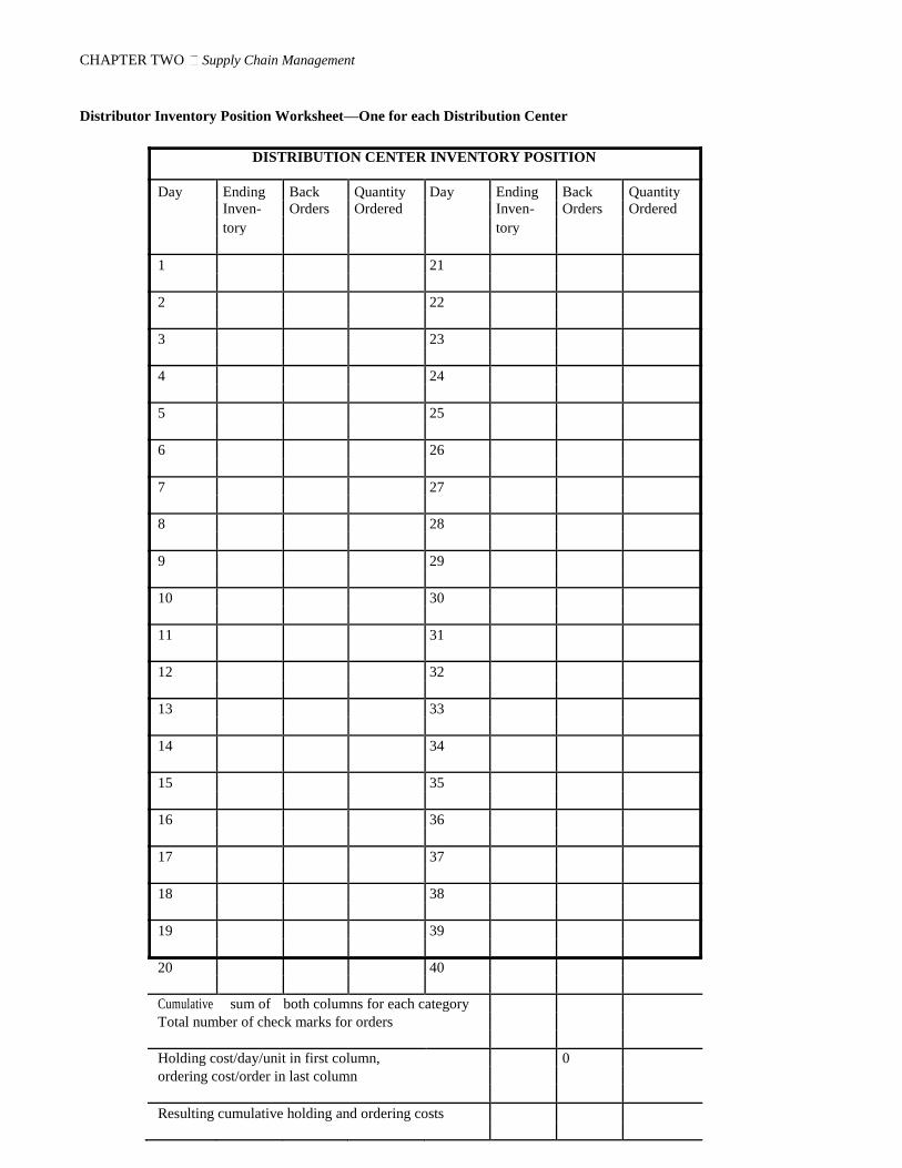
CHAPTER TWO Supply Chain Management
Distributor Inventory Position Worksheet—One for each Distribution Center
DISTRIBUTION CENTER INVENTORY POSITION
Day Ending Back Quantity Day Ending Back Quantity
Inven- Orders Ordered Inven- Orders Ordered
tory tory
1 21
2 22
3 23
4 24
5 25
6 26
7 27
8 28
9 29
10 30
11 31
12 32
13 33
14 34
15 35
16 36
17 37
18 38
19 39
20 40
Cumulative sum of both columns for each category
Total number of check marks for orders
Holding cost/day/unit in first column, 0
ordering cost/order in last column
Resulting cumulative holding and ordering costs

CHAPTER TWO Supply Chain
Management
Factory Inventory Position Worksheet
FACTORY INVENTORY POSITION
Day Ending Back Produc- Day Ending Back Produc-
Inven- Orders tion Inven- Orders tion
tory Order tory Order
1 21
2 22
3 23
4 24
5 25
6 26
7 27
8 28
9 29
10 30
11 31
12 32
13 33
14 34
15 35
16 36
17 37
18 38
19 39
20 40
Cumulative sum of both columns for each category
Total number of check marks for orders
Holding cost/day/unit in first column, 0
production order cost/order in last column
Resulting cumulative holding and ordering costs

Total operating cost (sum of both costs)
57

CHAPTER TWO Supply Chain Management
Forms for Multiple Product Versions: RETAIL STORE PURCHASE ORDER
Retailer: Day Sent: Day Rec.:
CD Artist: Quantity:
Jake Spade and the Diggers
The Heartmenders
Diamonds in the Ruff
Kulture Klub
RETAIL STORE PURCHASE ORDER
Retailer: Day Sent: Day Rec.:
CD Artist: Quantity:
Jake Spade and the Diggers
The Heartmenders
Diamonds in the Ruff
Kulture Klub
RETAIL STORE PURCHASE ORDER
Retailer: Day Sent: Day Rec.:
CD Artist: Quantity:
Jake Spade and the Diggers
The Heartmenders
Diamonds in the Ruff
Kulture Klub
RETAIL STORE PURCHASE ORDER
Retailer: Day Sent: Day Rec.:
CD Artist: Quantity:
Jake Spade and the Diggers
The Heartmenders
Diamonds in the Ruff
Kulture Klub
RETAIL STORE PURCHASE ORDER
Retailer: Day Sent: Day Rec.:
CD Artist: Quantity:
RETAIL STORE PURCHASE ORDER
Retailer: Day Sent: Day Rec.:
CD Artist: Quantity:
Jake Spade and the Diggers
The Heartmenders
Diamonds in the Ruff
Kulture Klub
RETAIL STORE PURCHASE ORDER
Retailer: Day Sent: Day Rec.:
CD Artist: Quantity:
Jake Spade and the Diggers
The Heartmenders
Diamonds in the Ruff
Kulture Klub
RETAIL STORE PURCHASE ORDER
Retailer: Day Sent: Day Rec.:
CD Artist: Quantity:
Jake Spade and the Diggers
The Heartmenders
Diamonds in the Ruff
Kulture Klub
RETAIL STORE PURCHASE ORDER
Retailer: Day Sent: Day Rec.:
CD Artist: Quantity: Jake Spade and the Diggers
The Heartmenders
Diamonds in the Ruff
Kulture Klub
Jake Spade and the Diggers
The Heartmenders
Diamonds in the Ruff
Kulture Klub

RETAIL STORE PURCHASE ORDER
Retailer: Day Sent: Day Rec.:
58 CD Artist: Quantity:
Jake Spade and the Diggers
The Heartmenders
Diamonds in the Ruff
Kulture Klub
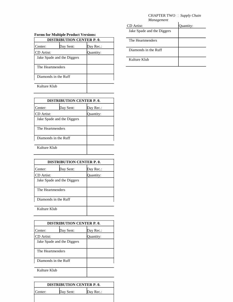
Forms for Multiple Product Versions: DISTRIBUTION CENTER P. 0.
Center: Day Sent: Day Rec.:
CD Artist: Quantity:
Jake Spade and the Diggers
The Heartmenders
Diamonds in the Ruff
Kulture Klub
DISTRIBUTION CENTER P. 0.
Center: Day Sent: Day Rec.:
CD Artist: Quantity:
Jake Spade and the Diggers
The Heartmenders
Diamonds in the Ruff
Kulture Klub
DISTRIBUTION CENTER P. 0.
Center: Day Sent: Day Rec.:
CD Artist: Quantity:
Jake Spade and the Diggers
The Heartmenders
Diamonds in the Ruff
Kulture Klub
DISTRIBUTION CENTER P. 0.
Center: Day Sent: Day Rec.:
CD Artist: Quantity:
Jake Spade and the Diggers
The Heartmenders
Diamonds in the Ruff
Kulture Klub
DISTRIBUTION CENTER P. 0.
Center: Day Sent: Day Rec.:
CHAPTER TWO Supply Chain
Management
CD Artist: Quantity:
Jake Spade and the Diggers
The Heartmenders
Diamonds in the Ruff
Kulture Klub

DISTRIBUTION CENTER P. 0.
Center: Day Sent: Day Rec.:
CD Artist: Quantity:
Jake Spade and the Diggers
The Heartmenders
Diamonds in the Ruff
Kulture Klub
DISTRIBUTION CENTER P. 0.
Center: Day Sent: Day Rec.:
CD Artist: Quantity:
Jake Spade and the Diggers
The Heartmenders
Diamonds in the Ruff
Kulture Klub
DISTRIBUTION CENTER P. 0.
Center: Day Sent: Day Rec.:
CD Artist: Quantity:
Jake Spade and the Diggers
The Heartmenders
Diamonds in the Ruff
Kulture Klub
DISTRIBUTION CENTER P. 0.
Center: Day Sent: Day Rec.:
CD Artist: Quantity:
Jake Spade and the Diggers
The Heartmenders
Diamonds in the Ruff
Kulture Klub
DISTRIBUTION CENTER P. 0.
Center: Day Sent: Day Rec.:
CD Artist: Quantity:
Jake Spade and the Diggers
The Heartmenders
Diamonds in the Ruff
Kulture Klub
59

CHAPTER TWO Supply Chain Management
Forms for Multiple Product Versions: FACTORY WORK ORDER
Day Placed: Day Complete:
CD Artist—Check One: Quantity:
Jake Spade and the Diggers
The Heartmenders
Diamonds in the Ruff
Kulture Klub
FACTORY WORK ORDER
Day Placed: Day Complete:
CD Artist—Check One: Quantity:
Jake Spade and the Diggers
The Heartmenders
Diamonds in the Ruff
Kulture Klub
FACTORY WORK ORDER
Day Placed: Day Complete:
CD Artist—Check One: Quantity:
Jake Spade and the Diggers
The Heartmenders
Diamonds in the Ruff
Kulture Klub
FACTORY WORK ORDER
Day Placed: Day Complete:
CD Artist—Check One: Quantity:
Jake Spade and the Diggers
The Heartmenders
Diamonds in the Ruff
Kulture Klub
FACTORY WORK ORDER
Day Placed: Day Complete:
CD Artist—Check One: Quantity:
Jake Spade and the Diggers
The Heartmenders
Diamonds in the Ruff
Kulture Klub
60
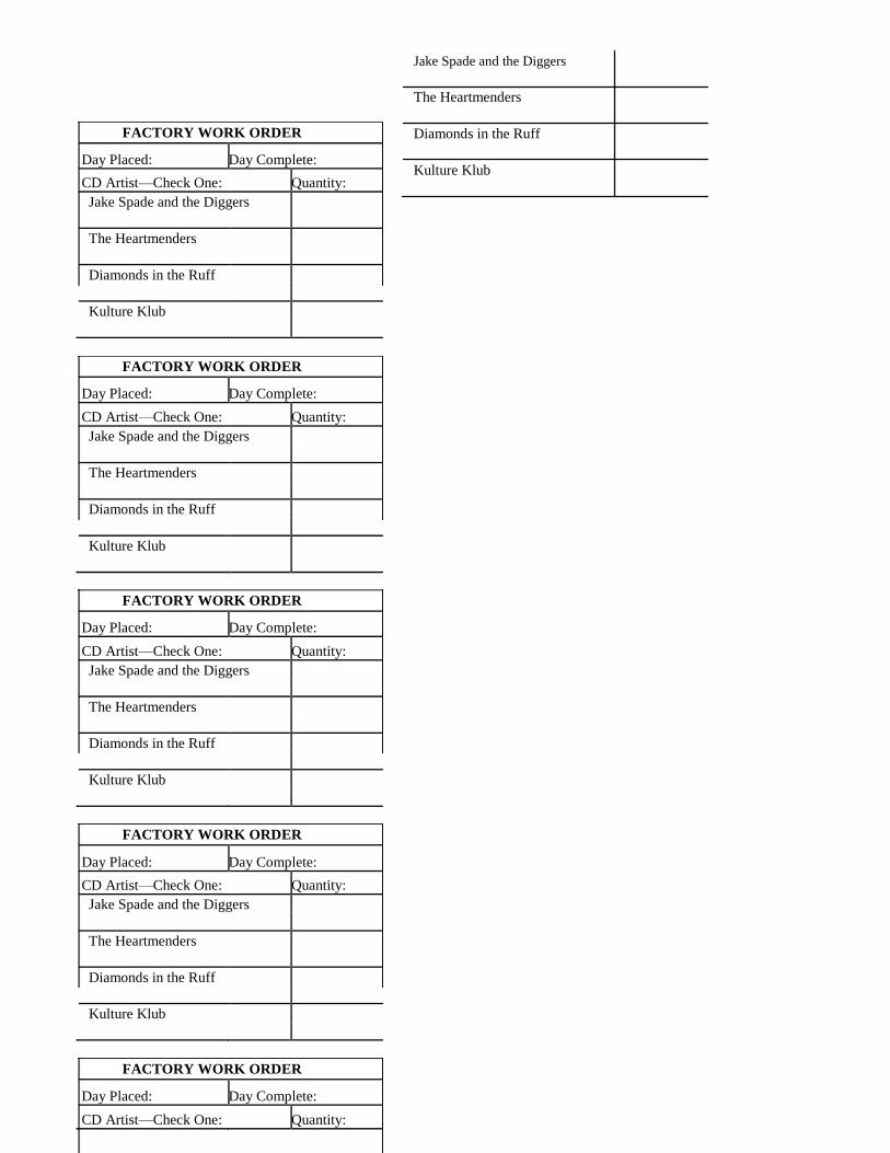
FACTORY WORK ORDER
Day Placed: Day Complete:
CD Artist—Check One: Quantity:
Jake Spade and the Diggers
The Heartmenders
Diamonds in the Ruff
Kulture Klub
FACTORY WORK ORDER
Day Placed: Day Complete:
CD Artist—Check One: Quantity:
Jake Spade and the Diggers
The Heartmenders
Diamonds in the Ruff
Kulture Klub
FACTORY WORK ORDER
Day Placed: Day Complete:
CD Artist—Check One: Quantity:
Jake Spade and the Diggers
The Heartmenders
Diamonds in the Ruff
Kulture Klub
FACTORY WORK ORDER
Day Placed: Day Complete:
CD Artist—Check One: Quantity:
Jake Spade and the Diggers
The Heartmenders
Diamonds in the Ruff
Kulture Klub
FACTORY WORK ORDER
Day Placed: Day Complete:
CD Artist—Check One: Quantity:
Jake Spade and the Diggers
The Heartmenders
Diamonds in the Ruff
Kulture Klub

CHAPTER TWO Supply Chain
Management
Forms for Multiple Product Versions: FACTORY MATL. DELIVERY FORM
To Cntr: Day Ship: Day Rec.:
CD Artist: Quantity:
Jake Spade and the Diggers
The Heartmenders
Diamonds in the Ruff
Kulture Klub
FACTORY MATL. DELIVERY FORM
To Cntr: Day Ship: Day Rec.:
CD Artist: Quantity:
Jake Spade and the Diggers
The Heartmenders
Diamonds in the Ruff
Kulture Klub
FACTORY MATL. DELIVERY FORM
To Cntr: Day Ship: Day Rec.:
CD Artist: Quantity:
Jake Spade and the Diggers
The Heartmenders
Diamonds in the Ruff
Kulture Klub
FACTORY MATL. DELIVERY FORM
To Cntr: Day Ship: Day Rec.:
CD Artist: Quantity:
Jake Spade and the Diggers
The Heartmenders
Diamonds in the Ruff
Kulture Klub
FACTORY MATL. DELIVERY FORM
To Cntr: Day Ship: Day Rec.:
CD Artist: Quantity:
Jake Spade and the Diggers
The Heartmenders
Diamonds in the Ruff
Kulture Klub
FACTORY MATL. DELIVERY FORM
To Cntr: Day Ship: Day Rec.:
CD Artist: Quantity:
Jake Spade and the Diggers
The Heartmenders
Diamonds in the Ruff
Kulture Klub
FACTORY MATL. DELIVERY FORM
To Cntr: Day Ship: Day Rec.:
CD Artist: Quantity:
Jake Spade and the Diggers
The Heartmenders
Diamonds in the Ruff
Kulture Klub
FACTORY MATL. DELIVERY FORM
To Cntr: Day Ship: Day Rec.:
FACTORY MATL. DELIVERY FORM
To Cntr: Day Ship: Day Rec.:
CD Artist: Quantity:
Jake Spade and the Diggers
The Heartmenders
Diamonds in the Ruff
Kulture Klub
CD Artist:
Quantity:
Jake Spade and the Diggers
The Heartmenders

Diamonds in the Ruff FACTORY MATL. DELIVERY FORM
To Cntr: Day Ship: Day Rec.:
Kulture Klub
CD Artist:
Quantity:
Jake Spade and the Diggers
The Heartmenders
Diamonds in the Ruff
Kulture Klub
61

CHAPTER TWO Supply Chain Management
Forms for Multiple Product Versions: DIST. CNTR. MATL. DELIV. FORM
To Store: Day Ship: Day Rec.:
CD Artist: Quantity:
Jake Spade and the Diggers
The Heartmenders
Diamonds in the Ruff
Kulture Klub
DIST. CNTR. MATL. DELIV. FORM
To Store: Day Ship: Day Rec.:
CD Artist: Quantity:
Jake Spade and the Diggers
The Heartmenders
Diamonds in the Ruff
Kulture Klub
DIST. CNTR. MATL. DELIV. FORM
To Store: Day Ship: Day Rec.:
CD Artist: Quantity:
Jake Spade and the Diggers
The Heartmenders
Diamonds in the Ruff
Kulture Klub
DIST. CNTR. MATL. DELIV. FORM
To Store: Day Ship: Day Rec.:
CD Artist: Quantity:
Jake Spade and the Diggers
The Heartmenders
Diamonds in the Ruff
Kulture Klub
DIST. CNTR. MATL. DELIV. FORM
To Store: Day Ship: Day Rec.:
CD Artist: Quantity:
Jake Spade and the Diggers
The Heartmenders
Diamonds in the Ruff
Kulture Klub
DIST. CNTR. MATL. DELIV. FORM
To Store: Day Ship: Day Rec.:
CD Artist: Quantity:
Jake Spade and the Diggers
The Heartmenders
Diamonds in the Ruff
Kulture Klub
DIST. CNTR. MATL. DELIV. FORM
To Store: Day Ship: Day Rec.:
CD Artist: Quantity:
Jake Spade and the Diggers
The Heartmenders
Diamonds in the Ruff
Kulture Klub
DIST. CNTR. MATL. DELIV. FORM
To Store: Day Ship: Day Rec.:
CD Artist: Quantity:
DIST. CNTR. MATL. DELIV. FORM
To Store: Day Ship: Day Rec.:
CD Artist: Quantity:
Jake Spade and the Diggers
The Heartmenders
Diamonds in the Ruff
Kulture Klub
Jake Spade and the Diggers
The Heartmenders
Diamonds in the Ruff

Kulture Klub DIST. CNTR. MATL. DELIV. FORM
To Store: Day Ship: Day Rec.:
CD Artist: Quantity:
Jake Spade and the Diggers
The Heartmenders
Diamonds in the Ruff
Kulture Klub
62

CHAPTER TWO Supply Chain
Management
Retailer Inventory Position Worksheet—One for each Retail Store
RETAIL STORE INVENTORY POSITION WORKSHEET RETAIL STORE #
Stock Stock
Ending Inventory - Order Ending Inventory - Order
outs Quantity outs Quantity
Day Day
1 21
2 22
3 23
4 24
5 25
6 26
7 27
8 28
9 29
10 30
11 31
12 32
13 33
14 34
15 35
16 36
17 37
18 38
19 39
20 40
Cumulative sum of both columns for each category
Total number of check marks for orders
Cost/unit (supplied by instructor).
Holding cost/day/unit in first four columns,
stockout cost (lost sale per unit) in fifth column,
ordering cost/order in last column

Cumulative holding, ordering, and stockout costs
Total operating cost (sum of all costs)
63

CHAPTER TWO Supply Chain Management
Distributor Inventory Position Worksheet—One for each Distribution Center
DISTRIBUTION CENTER CENTER #
INVENTORY POSITION WORKSHEET Ending
Inventory Back Order Ending Inventory Back Order
Order Order
s Quantity s Quantity
Day Day
1 21
2 22
3 23
4 24
5 25
6 26
7 27
8 28
9 29
10 30
11 31
12 32
13 33
14 34
15 35
16 36
17 37
18 38
19 39
20 40
Cumulative sum of both columns for each category
Total number of check marks for orders
Cost/unit (supplied by instructor) Holding cost/day/unit in first four columns, ordering cost/order in last column.

Resulting cumulative holding and ordering costs
Total operating cost (sum of all costs)
64
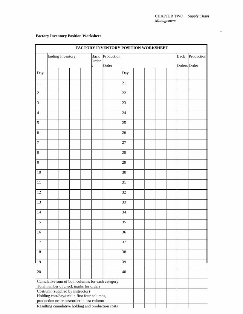
CHAPTER TWO Supply Chain
Management
Factory Inventory Position Worksheet
FACTORY INVENTORY POSITION WORKSHEET
Ending Inventory Back Production Back Production
Order
s Order Orders Order
Day Day
1 21
2 22
3 23
4 24
5 25
6 26
7 27
8 28
9 29
10 30
11 31
12 32
13 33
14 34
15 35
16 36
17 37
18 38
19 39
20 40
Cumulative sum of both columns for each category
Total number of check marks for orders
Cost/unit (supplied by instructor)
Holding cost/day/unit in first four columns,
production order cost/order in last column
Resulting cumulative holding and production costs

Total operating cost (sum of all costs)
65