General rights Copyright and moral rights for the publications made accessible in the public portal are retained by the authors and/or other copyright owners and it is a condition of accessing publications that users recognise and abide by the legal requirements associated with these rights.

Users may download and print one copy of any publication from the public portal for the purpose of private study or research.

You may not further distribute the material or use it for any profit-making activity or commercial gain

You may freely distribute the URL identifying the publication in the public portal If you believe that this document breaches copyright please contact us providing details, and we will remove access to the work immediately and investigate your claim.

Downloaded from orbit.dtu.dk on: Aug 13, 2020

Solubility of syngas components in water acetic acid and alcohol using new standardfugacity methodology

Torli, Mauro; Geer, Luydmila; Kontogeorgis, Georgios M.; Fosbøl, Philip L.

Published in:Industrial and Engineering Chemistry Research

Link to article, DOI:10.1021/acs.iecr.8b03954

Publication date:2018

Document VersionPeer reviewed version

Link back to DTU Orbit

Citation (APA):Torli, M., Geer, L., Kontogeorgis, G. M., & Fosbøl, P. L. (2018). Solubility of syngas components in water aceticacid and alcohol using new standard fugacity methodology. Industrial and Engineering Chemistry Research, 57,16958–16977. https://doi.org/10.1021/acs.iecr.8b03954

Solubility of syngas components in water acetic acid

and alcohol using new standard fugacity

methodology

Mauro Torli, Luydmila Geer, Georgios M. Kontogeorgis, Philip L. Fosbøl*

Center for Energy Resources Engineering (CERE), Department of Chemical and Biochemical

Engineering, Technical University of Denmark, DK-2800 Lyngby, Denmark

Keywords: Vapor-liquid equilibria; gas solubility; Henry’s law constant; solubility in mixed

solvents; UNIQUAC; ethanol; water; acetic acid; CO2; CO; CH4; N2; H2

Abstract: The UNIQUAC model in combination with the Peng-Robinson and the Hayden-

O'Connell Virial equation of state was used for correlating vapor-liquid equilibrium for a gas-

solvent system containing: CO2-Water, CO2-Ethanol, CO2-Acetic acid, CO-Water, CO-Ethanol,

CO-Acetic acid, CH4-Water, CH4-Ethanol, CH4-Acetic acid, N2-Water, N2-Ethanol, N2-Acetic

acid, H2-Water, H2-Ethanol. Prausnitz and Shair correlation, for the fugacity of the hypothetical

liquid solute at a pressure of 1 atm, was implemented in the parametrization procedure as

additional objective function so as to reduce the uncertainty on the constants of the model. The

results show that the UNIQUAC equation, coupled with an appropriate equation of state to

model the vapor phase non ideality, is able to represent the binaries in the range of temperatures

and pressures considered in the study, i.e. from 0 to 310 °C, and from 1 to 400 bar, respectively.

1

In addition to model parameter estimation, a new generic method to evaluate gas solubility in

mixed solvents based on the thermodynamic relation of Henry’s law constant with the activity

coefficient at infinite dilution, has been derived. Provided the binary parameters of a generic

excess Gibbs energy model, the gas solubility in the multicomponent system can be readily

estimated.

2

1 Introduction

There is in today’s society an increasing focus towards production of greener fuels and

chemicals which do not originate from fossil fuels. One way to accomplish this is by using

synthesis gas (syngas) as a resource. Today, syngas is mainly produced from thermal gasification

of coal and natural gas steam reforming. Uses of syngas include methanol synthesis, hydrogen

production for ammonia and oil refineries, Fischer-Tropsch fuels, iron reduction and power

generation. There is an increasing need to use more green resources for syngas formation.

Therefore, syngas obtained from thermal gasification of biomass has grown substantially in the

last decades 1.

The focus of this work is on green syngas fermentation. It is one of several emerging

technologies for the production of biofuels from renewable sources. In this process biomass is

gasified to syngas (CO and H2), which is then fermented by acetogenic bacteria to produce

ethanol, acetic acid or other chemical commodities 2.

The rate-limiting step of syngas fermentation is the gas-to-liquid mass transfer, and mass

transfer limitations are expected to be even more severe than in the ordinary aerobic fermentation

based on glucose. Indeed, CO and H2 solubilities are only 60% and 4% of O2, and more moles of

gas must be transferred per carbon equivalent consumed. One way to improve the mass transfer

is to increasing the mass transfer driving force. This is accomplished by raising the partial

pressure of the syngas 3. In order to estimate the equilibrium condition at high solute

concentration, the Henry’s law is not sufficient, especially above 5-10 bar and for molar fractions

larger than 0.03 4.

A widely studied example of a supercritical component in polar associating solvent is CO2-

H2O. Carroll and Mather (1992) 5 provide a historical overview of this system. The simple

3

Krichevsky-Kasarnovsky approach was found to be valid up to about 100 bar; the modified

Krichevsky-Ilinskaya approach, where the un-symmetric activity coefficient is estimated using

Margules equations 6, made the modelling valid up to 1000 bar.

Another 𝛾𝛾 − 𝜑𝜑 approach was applied by Duan and Sun (2003) 7 to the more complex CO2-

brine system up to 2000 bar. Pitzer equation 8 was used for the non-ideal liquid behavior.

With the introduction of Huron-Vidal mixing rules (1979) 9, it became possible to combine the

advantages of cubic equation of state (EoS) with activity coefficient models in order to have a

framework valid both at very high pressures and for polar compounds that exhibit high

deviations from ideality in the liquid phase. An application of this method to the system CO2-

H2O can be found in the study of Pedersen et al. (2001) 10.

Another approach to thermodynamic modelling of complex mixtures is the Cubic-Plus

Association (CPA) equation of state, introduced by Kontogeorgis et al. (1996) 11 to account for

the effect of hydrogen-bonds and related phenomena. CPA is based on a cubic equation, usually

the Soave-Redlich-Kwong (SRK) EoS, and the association term is taken from SAFT (Statistical

Associating Fluid Theory 12). The equation have been used to model CO2-H2O and/or ternaries

systems containing the two components first in 2006 by Kontogeorgis et al. 13 Austegard et al. 14

and Perakis et al. 15. By now several thermodynamic studies have been published on CO2-H2O

and related systems. Many of these studies apply CPA for all phases, but some still use 𝛾𝛾 − 𝜑𝜑

approach even at relative high pressure conditions, e.g. García et al. (2006) 16, Spycher and

Pruess (2010) 17, Hou et al. (2013) 18, Mao et al. (2013) 19 and Venkatraman et al. (2014) 20.

In this work we focus on the thermodynamic of 15 systems which may be of relevance for

process simulation studies in connection with the biological synthesis of solvents, chemicals or

the production of biofuels from syngas. A thermodynamic model is presented which describes

4

the solubility of CO, H2, CO2, CH4 and N2, i.e. the main component of biomass derived syngas,

in combination with the three polar hydrogen bonding solvents: water, ethanol and acetic acid.

The selected method is 𝛾𝛾 − 𝜑𝜑 approach: UNIQUAC-Peng-Robinson (PR) for system containing

water and ethanol, and UNIQUAC-Hayden-O'Connell Virial EoS for systems containing acetic

acid. An explanation of the modelling, using a mix of PR and Hayden-O'Connell for the gas

phase, is discussed in section 3.

The data regression has been performed with additional constraints on the supercritical

component standard state fugacities and, on the same thermodynamic basis; a new approach for

gas solubility in mixed solvents has been derived. This approach has been implemented in order

to avoid the derivation of ill-defined UNIQUAC parameters that are merely correlations and

produce wrong property prediction of particularly 𝛾𝛾∞. Indeed there is a need for future

researches to address the fact that a consistent thermodynamic framework should be adopted

whenever the 𝛾𝛾 − 𝜑𝜑 approach is applied to gas solubility.

The gas solubility equilibria investigated in this study are of particular relevance to the syngas

fermentation process, however they are also central to many other industrial applications, such

as: ethanol and acetic acid fermentation, carbonation of alcoholic beverages and soft drinks, gas

absorption, stripping columns, waste-water treatment, etc. 21

2 Theory of the applied thermodynamic modeling

2.1 The 𝜸𝜸 − 𝝋𝝋 approach close to the critical conditions

The 𝛾𝛾 − 𝜑𝜑 approach has been used, and is still used, to successfully correlate solubility data

also at high pressure. It is often stated that the concept cannot be used at high pressure due to

various limitations and here we highlight some of the concerns in the existing activity coefficient

models which are not present when using EoS’.

5

Though there are some exceptions 22, activity coefficient model are in general pressure

independent expressions 23 and they cannot account for the effect of this variable on the excess

Gibbs energy 𝐺𝐺𝐸𝐸 of the system. This is equivalent to not considering the change in volume upon

mixing, 𝑉𝑉𝐸𝐸 ≅ 0, as indicate in Eq. (1).

; 0E E E Ei ii

dG S dT dn V dPµ− +∑ (1)

The contribution of the term ∫𝑉𝑉𝐸𝐸 𝑑𝑑𝑑𝑑 to the excess Gibbs energy 𝐺𝐺𝐸𝐸 may become important at

high pressure for systems with very large excess volumes. Nevertheless the practical limitations

with the 𝛾𝛾 − 𝜑𝜑 approach are due to the incorrect estimates on standard state liquid fugacities for

components near critical conditions, rather than neglecting the pressure effect on 𝐺𝐺𝐸𝐸.

The standard state liquid fugacities at 𝑇𝑇 and 𝑑𝑑 are obtained from the saturation (vapor)

pressure at 𝑇𝑇 applying two corrections: 1.A fugacity coefficient at saturated conditions,

𝜑𝜑𝑖𝑖𝐿𝐿(𝑇𝑇)�𝑃𝑃𝑖𝑖𝑠𝑠𝑠𝑠𝑠𝑠 usually calculated from an EoS, to take into account the deviations of the saturated

vapor from ideal-gas behavior. 2.A Poynting factor since the liquid is at a pressure 𝑑𝑑 different

from the one at saturation. This term is related to the difference between the fugacity at standard

state conditions, 𝑓𝑓𝑖𝑖𝐿𝐿(𝑇𝑇,𝑑𝑑), and the fugacity at the saturation line, 𝑓𝑓𝑖𝑖𝐿𝐿(𝑇𝑇)�𝑃𝑃𝑖𝑖𝑠𝑠𝑠𝑠𝑠𝑠.

The rigorous form of the Poynting correction requires the calculation the integral term

∫ 𝜐𝜐𝑖𝑖𝐿𝐿 𝑑𝑑𝑑𝑑; however a condensed phase at conditions far from critical, may often be regarded as

incompressible, and in that case the Poynting term takes a simpler form where the integral term

is replaced by the product of an invariant molar volume and the pressures difference between the

extremes of integration 𝑑𝑑 and 𝑑𝑑𝑖𝑖𝑠𝑠𝑠𝑠𝑠𝑠. This simplified form is the one used in practice, therefore

excess Gibbs energy models are applicable as long as this assumption holds 4.

6

2.2 Theory of un-symmetric standard state

Gases used in the 𝛾𝛾 − 𝜑𝜑 approach are commonly treated according to the un-symmetric

convention, this is because the pure components liquid properties for the given 𝑇𝑇 cannot be

measured.

In this section we describe the theory used in the application of the un-symmetric framework.

A description is given on how the Henry’s law constant at standard conditions and the Henry’s

law constant at solvent saturation pressure are defined and linked.

For super critical components, relations based on the symmetric approach can only be used by

introducing a hypothetical (physically unreal) liquid standard state.

In order to avoid difficulties, whenever the liquid mixture cannot exist over the entire

composition range, it is common practice to define excess functions relative to an ideal dilute

solution, in line with Henry’s law. The condition for ideality requires the ratio of the fugacity to

the solute mole fraction being independent on its concentration; which is the case, provided the

latter is sufficiently small. Accordingly, for a component under the un-symmetric convention the

standard state is specified by unit concentration extrapolated to the limit of infinite dilution.

The Henry’s law constant, 𝐻𝐻𝑔𝑔(𝑇𝑇,𝑑𝑑,𝐧𝐧𝒌𝒌)𝑘𝑘≠𝑔𝑔, is defined as the limit ratio of the fugacity of the

component in the vapor phase and its mole fraction in the solution when the latter tends to zero,

Eq. (2). Its value can be obtained from the one at 𝑇𝑇 and 𝑑𝑑𝑠𝑠𝑠𝑠𝑠𝑠𝑠𝑠𝑠𝑠𝑠𝑠, 𝐻𝐻𝑔𝑔(𝑇𝑇,𝐧𝐧𝒌𝒌)𝑘𝑘≠𝑔𝑔�𝑃𝑃𝑠𝑠𝑠𝑠𝑠𝑠𝑠𝑠𝑠𝑠𝑠𝑠, applying the

Poynting correction, Eq. (3).

0 0

( , , ) ˆ( , , ) = lim lim ( , , )g g

Vg gV

g k k g gx xg g

yf T PH T P P T Px x

ϕ≠ → →=

mn m (2)

1( , , ) ( , ) exp satsatsolsol

P

g k k g g k k g gPPH T P H T dP

RTυ ∞

≠ ≠

=

∫n n (3)

7

Solubility measurements require two phases always present; as the limit 𝑥𝑥𝑔𝑔 → 0 is approached,

𝑦𝑦𝑔𝑔 goes to zero as well, and the pressure of the system tends to the vapor pressure of the solvent

alone: 𝑑𝑑 → 𝑑𝑑𝑠𝑠𝑠𝑠𝑠𝑠𝑠𝑠𝑠𝑠𝑠𝑠. In this case the extremes of integration in the Poynting correction overlap and

the Henry’s law constant matches the value at solvent saturation pressure 24. Measurements of

total pressure and composition of both phases are preferably needed, plus the fugacity

coefficients from an EoS, Eq. (2).

In the most rigorous way the determination of the Henry’s law constant at solvent saturation

pressure, requires measurements to the lowest mole fractions possible so as to reduce the extent

of extrapolation at 𝑥𝑥𝑔𝑔 → 0; for obvious reasons solubilities are never measured at those

conditions.

In order to represent solubility equilibria at different pressures, it is possible to extend the

validity of Eq. (2) outside the limit condition of infinite dilution. Krichevsky-Kasarnovsky

equation 25, Eq. (4) can be derived upon combining Eq. (2) and (3), for pure solvent, and by

considering �̅�𝜐𝑔𝑔∞ constant with pressure (a reasonable assumption if the solution temperature is

well below critical conditions).

( )ˆln ( , , ) ln ( ) ;sat

i

g gV satg g iP

g

yP T P pure solvent cH T P P

x RTase

υϕ

∞ = + − m (4)

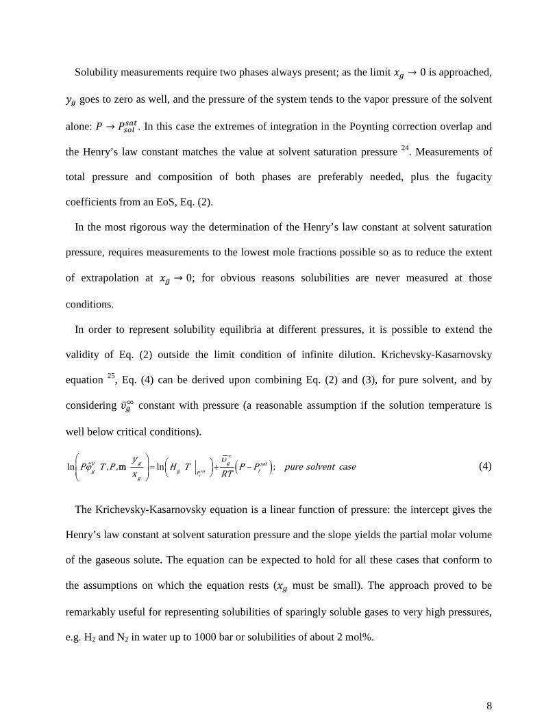
The Krichevsky-Kasarnovsky equation is a linear function of pressure: the intercept gives the

Henry’s law constant at solvent saturation pressure and the slope yields the partial molar volume

of the gaseous solute. The equation can be expected to hold for all these cases that conform to

the assumptions on which the equation rests (𝑥𝑥𝑔𝑔 must be small). The approach proved to be

remarkably useful for representing solubilities of sparingly soluble gases to very high pressures,

e.g. H2 and N2 in water up to 1000 bar or solubilities of about 2 mol%.

8

At larger solubilities, deviations become significant. In those cases, the non-ideality (in the

sense of Henry’s law 4) can be accounted using an activity coefficient and replacing 𝑥𝑥𝑔𝑔 in Eq. (4)

with the product 𝛾𝛾𝑔𝑔∗(𝑇𝑇,𝐧𝐧)𝑥𝑥𝑔𝑔 which gives.

( ) ( )ˆln ( , , ) ln ( , ) ln ( , )sat

sol

g gV satg g k k g g solP

g

yP T P H T T P P

x RTυ

ϕ γ∞

∗≠

= + + − m n n (5)

When the two-suffix Margules equation6 is used to model the un-symmetric activity coefficient

in a pure solvent, the general form of Eq. (5) leads to Krichevsky-Ilinskaya equation, Eq. (6).

( ) ( )2( )ˆln ( , , ) ln ( ) 1 ; sat

i

g gV satg g i iP

g

pure solventy A TP T P H T x P Px RT RT

caseυ

ϕ∞ = + − + −

m (6)

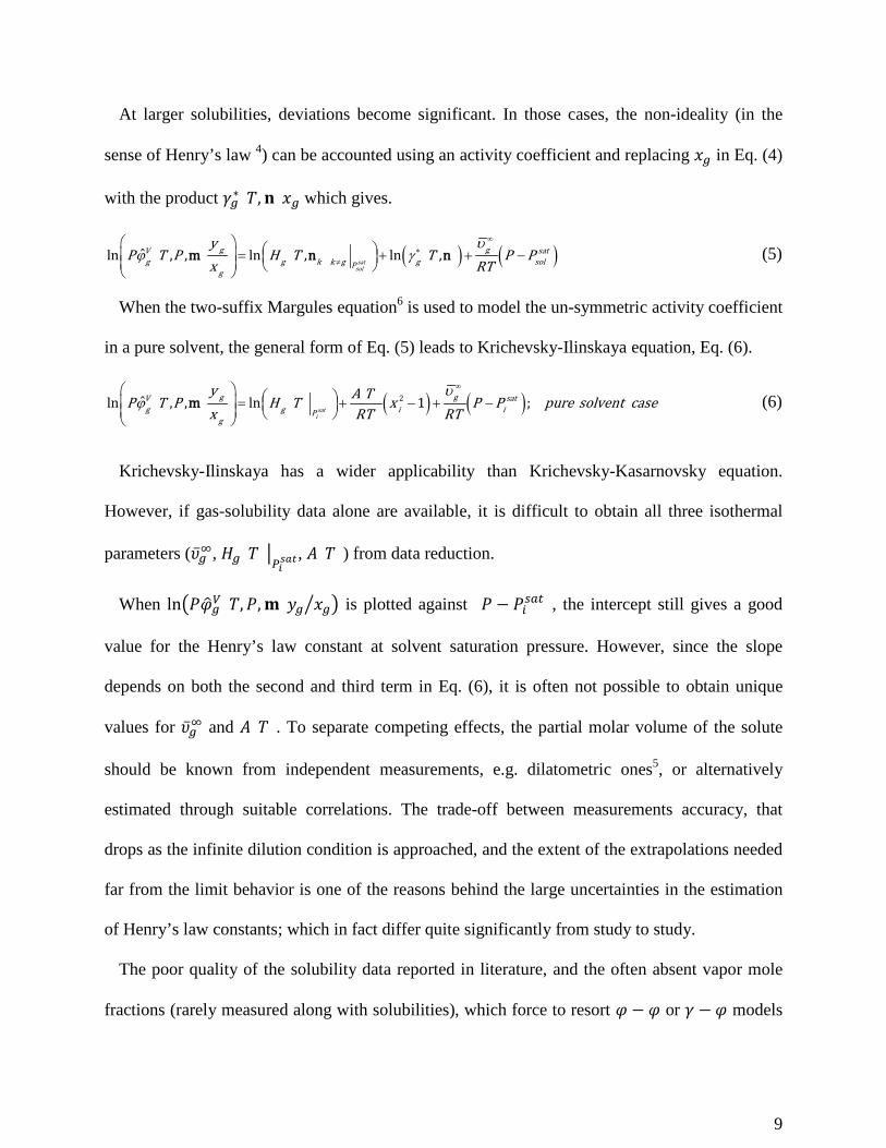
Krichevsky-Ilinskaya has a wider applicability than Krichevsky-Kasarnovsky equation.

However, if gas-solubility data alone are available, it is difficult to obtain all three isothermal

parameters (�̅�𝜐𝑔𝑔∞, 𝐻𝐻𝑔𝑔(𝑇𝑇)�𝑃𝑃𝑖𝑖𝑠𝑠𝑠𝑠𝑠𝑠, 𝐴𝐴(𝑇𝑇)) from data reduction.

When ln�𝑑𝑑𝜑𝜑�𝑔𝑔𝑉𝑉(𝑇𝑇,𝑑𝑑,𝐦𝐦)𝑦𝑦𝑔𝑔 𝑥𝑥𝑔𝑔� � is plotted against (𝑑𝑑 − 𝑑𝑑𝑖𝑖𝑠𝑠𝑠𝑠𝑠𝑠), the intercept still gives a good

value for the Henry’s law constant at solvent saturation pressure. However, since the slope

depends on both the second and third term in Eq. (6), it is often not possible to obtain unique

values for �̅�𝜐𝑔𝑔∞ and 𝐴𝐴(𝑇𝑇). To separate competing effects, the partial molar volume of the solute

should be known from independent measurements, e.g. dilatometric ones5, or alternatively

estimated through suitable correlations. The trade-off between measurements accuracy, that

drops as the infinite dilution condition is approached, and the extent of the extrapolations needed

far from the limit behavior is one of the reasons behind the large uncertainties in the estimation

of Henry’s law constants; which in fact differ quite significantly from study to study.

The poor quality of the solubility data reported in literature, and the often absent vapor mole

fractions (rarely measured along with solubilities), which force to resort 𝜑𝜑 − 𝜑𝜑 or 𝛾𝛾 − 𝜑𝜑 models

9

to estimate the equilibrium (vapor) compositions make the estimation of Henry’s law constants

even more problematic.

2.3 Links between saturation pressure and Henry’s law constant

Saturation pressures of pure liquids are measured at the very conditions defined by the

corresponding saturation lines. In contrast the Henry’s law constants at the solvent saturation

pressure conditions are calculated (not measured) from low pressure data under simplified

assumptions, or obtained from data regression according to the Krichevsky-Kasarnovsky

equation, Krichevsky-Ilinskaya equation or Eq. (5). Though the correlation schemes to some

extent affect the 𝐻𝐻𝑔𝑔(𝑇𝑇)�𝑃𝑃𝑖𝑖𝑠𝑠𝑠𝑠𝑠𝑠 values, it is generally possible to get an acceptable estimation, even

with great uncertainty on the rest of the parameters (�̅�𝜐𝑔𝑔∞, 𝐴𝐴(𝑇𝑇), or the interaction parameters for

the activity coefficient model adopted for Eq. (5)). At this regard, Carroll and Mather 5 give an

example of an hypothetical system that produces a linear trend in the Krichevsky-Kasarnovsky

plot. Such behavior makes it difficult to separate the contributions of �̅�𝜐𝑔𝑔∞ and 𝐴𝐴(𝑇𝑇) on the gas

solubility (as function of pressure), i.e. the two parameters are nearly indeterminate. Carroll and

Mather further report that solubility data showing negative slopes in the Krichevsky-

Kasarnovsky plot have led, not in a few cases, to the erroneous assumption of a negative υ�g∞.

All things considered, the Henry’s law constant at the solvent saturation pressure (that

corresponds to the intercept of 𝑓𝑓𝑔𝑔𝑉𝑉(𝑇𝑇,𝑑𝑑,𝐦𝐦) in the Krichevsky-Kasarnovsky plot), is only partly

influenced by the uncertainty on the model parameters. Indeed, 𝐻𝐻𝑔𝑔(𝑇𝑇)�𝑃𝑃𝑖𝑖𝑠𝑠𝑠𝑠𝑠𝑠 is always explicitly

calculated and defined in the limit of infinite dilution where the activity coefficient and Poynting

term do not play a role. This attests that the Henry’s law constant at the saturation pressure of the

solvent it is not a parameter whose value can be freely tuned to improve data fitting of a possibly

poor thermodynamic modeling.

10

Indeed, 𝐻𝐻𝑔𝑔(𝑇𝑇)�𝑃𝑃𝑖𝑖𝑠𝑠𝑠𝑠𝑠𝑠 is a property of the un-symmetric state: �𝑇𝑇,𝑑𝑑𝑖𝑖𝑠𝑠𝑠𝑠𝑠𝑠 , 𝑥𝑥𝑔𝑔 → 0� and just like the

symmetric fugacity 𝑓𝑓𝑖𝑖𝐿𝐿(𝑇𝑇)�𝑃𝑃𝑖𝑖𝑠𝑠𝑠𝑠𝑠𝑠 , has some fundamental characteristics. 𝐻𝐻𝑔𝑔(𝑇𝑇)�

𝑃𝑃𝑖𝑖𝑠𝑠𝑠𝑠𝑠𝑠 and 𝑓𝑓𝑖𝑖𝐿𝐿(𝑇𝑇)�

𝑃𝑃𝑖𝑖𝑠𝑠𝑠𝑠𝑠𝑠

are functions of temperature only, both describe a vapor-liquid equilibrium and they can be

correlated with the inverse of temperature in the Van't Hoff plot. The slope of the resulting

curves yield respectively: the evaporation enthalpies, or the dissolution enthalpies. For pure

liquid saturated vapor pressure, the corresponding expressions are known as Antoine equations,

as the most general form adopted by AspenTech 26 and reported Eq. (7), while the simplest one is

the Clausius-Clapeyron relation. For the Henry’s law constant in a pure solvent at its saturation

pressure, similar functions of temperature are used; e.g. Eq. (8) found in AspenTech software 26

and applied in several works on gas solubility, it was first developed by Glew 27.

In this work a truncated form of Eq. (8), using the first three terms, was found appropriate to

represent the variation of the Henry’s law constant with temperature; also in view of the quality

of the data and the consequential uncertainty on the actual value of 𝐻𝐻𝑔𝑔(𝑇𝑇)�𝑃𝑃𝑖𝑖𝑠𝑠𝑠𝑠𝑠𝑠.

( ) ( ) ( ) 721 4 5 6

3

ln / bar ln psati

pP p p T p T p T

T p= + + + +

+ (7)

( ) 521 3 4 2

ln ( ) / bar ln ;sat

ig P

hhH T h h T h pure solvent casT

Te

T = + + + +

(8)

2.4 Hypothetical standard state fugacity for supercritical components

In gas solubility calculations, the gas is often in a supercritical condition and it therefore

cannot exist in a condensed state, if not as a solute in a mixture. For the same reason pure

saturated vapor pressures do not exist, making it impossible to define the corresponding

fugacities at the saturation line, (𝑇𝑇,𝑑𝑑𝑖𝑖𝑠𝑠𝑠𝑠𝑠𝑠).

11

In order to model gas solubility according to the symmetric convention, a hypothetical liquid

standard state, which assumes that the pure condensed gas can exist, is formally introduced,

𝑓𝑓𝑔𝑔ℎ𝑦𝑦𝐿𝐿(𝑇𝑇,𝑑𝑑). The fugacity of the component in the mixture can, therefore, be equivalently

expressed by Eq. (9) or Eq. (10); respectively according to symmetric and the un-symmetric

convention.

ˆ ( , , ) ( , ) ( , )V hyLg g g gf T P f T P x Tγ=n n (9)

ˆ ( , , ) ( , , ) ( , )Vg g k k g g gf T P H T P x Tγ ∗

≠=n n n (10)

Equating Eq. (9) and Eq. (10) at the limit of 𝑥𝑥𝑔𝑔 → 0 leads to:

0 0( , , ) lim ( , ) ( , ) lim ( , )

g g

hyLg k k g g g g g gx x

H T P x T f T P x Tγ γ∗≠ → →

= ⇒n n n (11)

( , , )( , )

( , )g k k g hyL

gg k k g

H T Pf T P

Tγ≠

∞≠

=n

n (12)

Both the symmetric activity coefficient at infinite dilution, 𝛾𝛾𝑔𝑔∞(𝑇𝑇,𝐧𝐧𝑘𝑘)𝑘𝑘≠𝑔𝑔, and the Henry’s law

constant, 𝐻𝐻𝑔𝑔(𝑇𝑇,𝐧𝐧𝑘𝑘)𝑘𝑘≠𝑔𝑔, depend on the nature of the solute-solvent interaction. Their ratio,

𝐻𝐻𝑔𝑔(𝑇𝑇,𝑑𝑑,𝐧𝐧𝑘𝑘)𝑘𝑘≠𝑔𝑔 𝛾𝛾𝑔𝑔∞(𝑇𝑇,𝐧𝐧𝑘𝑘)𝑘𝑘≠𝑔𝑔⁄ , is a property of the gaseous component alone, and it must be

identical in any solvent or solvent mixture 23.

The introduction of 𝑓𝑓𝑔𝑔ℎ𝑦𝑦𝐿𝐿(𝑇𝑇,𝑑𝑑), into the left hand side of Eq. (11) yields the relation between

symmetric and un-symmetric activity coefficients:

( , )( , )

( , )g

gg k k g

TT

Tγ

γγ

∗∞

≠

=n

nn

(13)

Eq. (13) allows for the use of symmetric activity models in the un-symmetric approach.

However, the resulting formulas are affected by large uncertainty regarding the parameterization,

especially for systems of sparingly soluble gases. This can be exemplified by rewriting Eq. (13)

in terms of the three-suffix Margules equations, i.e.:

12

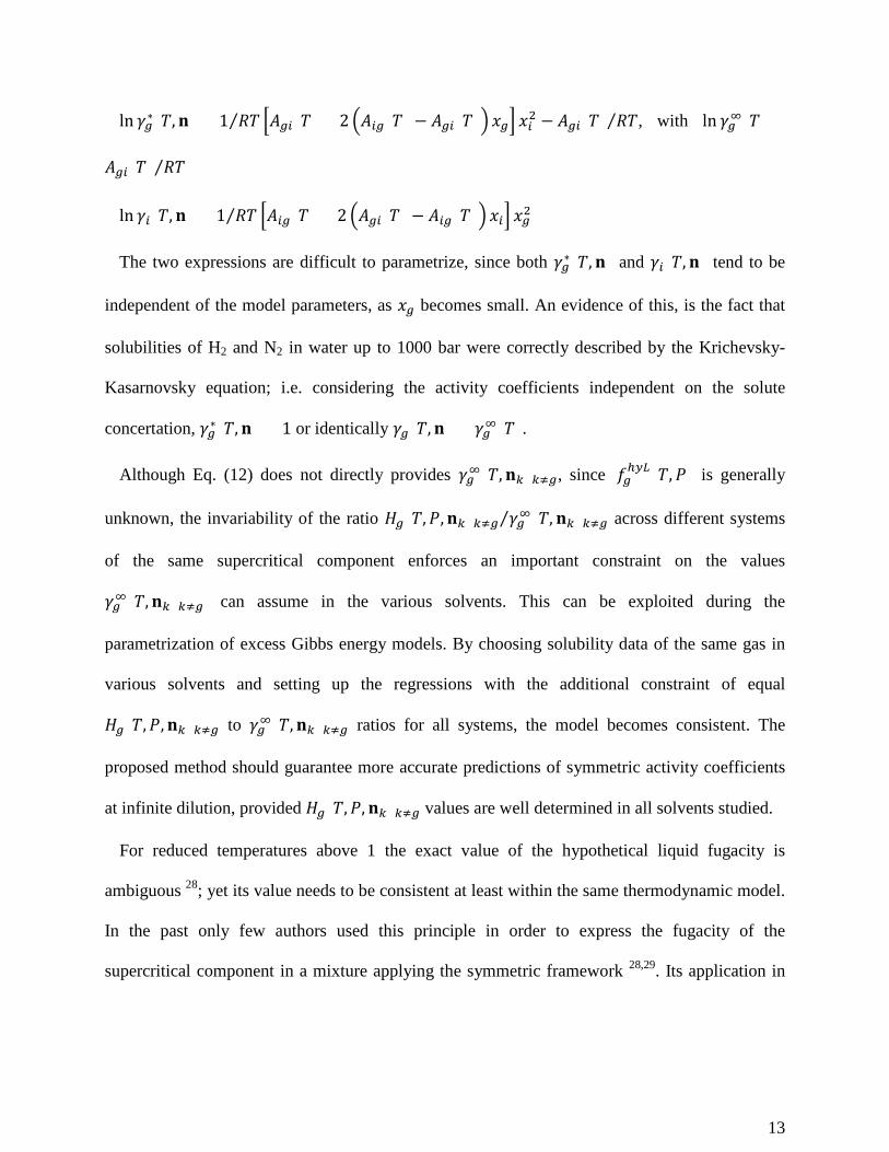
ln 𝛾𝛾𝑔𝑔∗(𝑇𝑇,𝐧𝐧) = 1 𝑅𝑅𝑇𝑇⁄ �𝐴𝐴𝑔𝑔𝑖𝑖(𝑇𝑇) + 2 �𝐴𝐴𝑖𝑖𝑔𝑔(𝑇𝑇) − 𝐴𝐴𝑔𝑔𝑖𝑖(𝑇𝑇)� 𝑥𝑥𝑔𝑔� 𝑥𝑥𝑖𝑖2 − 𝐴𝐴𝑔𝑔𝑖𝑖(𝑇𝑇) 𝑅𝑅𝑇𝑇⁄ , with ln 𝛾𝛾𝑔𝑔∞(𝑇𝑇) =

𝐴𝐴𝑔𝑔𝑖𝑖(𝑇𝑇) 𝑅𝑅𝑇𝑇⁄

ln 𝛾𝛾𝑖𝑖(𝑇𝑇,𝐧𝐧) = 1 𝑅𝑅𝑇𝑇⁄ �𝐴𝐴𝑖𝑖𝑔𝑔(𝑇𝑇) + 2 �𝐴𝐴𝑔𝑔𝑖𝑖(𝑇𝑇) − 𝐴𝐴𝑖𝑖𝑔𝑔(𝑇𝑇)� 𝑥𝑥𝑖𝑖� 𝑥𝑥𝑔𝑔2

The two expressions are difficult to parametrize, since both 𝛾𝛾𝑔𝑔∗(𝑇𝑇,𝐧𝐧) and 𝛾𝛾𝑖𝑖(𝑇𝑇,𝐧𝐧) tend to be

independent of the model parameters, as 𝑥𝑥𝑔𝑔 becomes small. An evidence of this, is the fact that

solubilities of H2 and N2 in water up to 1000 bar were correctly described by the Krichevsky-

Kasarnovsky equation; i.e. considering the activity coefficients independent on the solute

concertation, 𝛾𝛾𝑔𝑔∗(𝑇𝑇,𝐧𝐧) = 1 or identically 𝛾𝛾𝑔𝑔(𝑇𝑇,𝐧𝐧) = 𝛾𝛾𝑔𝑔∞(𝑇𝑇).

Although Eq. (12) does not directly provides 𝛾𝛾𝑔𝑔∞(𝑇𝑇,𝐧𝐧𝑘𝑘)𝑘𝑘≠𝑔𝑔, since 𝑓𝑓𝑔𝑔ℎ𝑦𝑦𝐿𝐿(𝑇𝑇,𝑑𝑑) is generally

unknown, the invariability of the ratio 𝐻𝐻𝑔𝑔(𝑇𝑇,𝑑𝑑,𝐧𝐧𝑘𝑘)𝑘𝑘≠𝑔𝑔 𝛾𝛾𝑔𝑔∞(𝑇𝑇,𝐧𝐧𝑘𝑘)𝑘𝑘≠𝑔𝑔⁄ across different systems

of the same supercritical component enforces an important constraint on the values

𝛾𝛾𝑔𝑔∞(𝑇𝑇,𝐧𝐧𝑘𝑘)𝑘𝑘≠𝑔𝑔 can assume in the various solvents. This can be exploited during the

parametrization of excess Gibbs energy models. By choosing solubility data of the same gas in

various solvents and setting up the regressions with the additional constraint of equal

𝐻𝐻𝑔𝑔(𝑇𝑇,𝑑𝑑,𝐧𝐧𝑘𝑘)𝑘𝑘≠𝑔𝑔 to 𝛾𝛾𝑔𝑔∞(𝑇𝑇,𝐧𝐧𝑘𝑘)𝑘𝑘≠𝑔𝑔 ratios for all systems, the model becomes consistent. The

proposed method should guarantee more accurate predictions of symmetric activity coefficients

at infinite dilution, provided 𝐻𝐻𝑔𝑔(𝑇𝑇,𝑑𝑑,𝐧𝐧𝑘𝑘)𝑘𝑘≠𝑔𝑔 values are well determined in all solvents studied.

For reduced temperatures above 1 the exact value of the hypothetical liquid fugacity is

ambiguous 28; yet its value needs to be consistent at least within the same thermodynamic model.

In the past only few authors used this principle in order to express the fugacity of the

supercritical component in a mixture applying the symmetric framework 28,29. Its application in

13

the customary un-symmetric approach to prevent thermodynamic inconsistency and wrong

property prediction of particularly 𝛾𝛾𝑔𝑔∞(𝑇𝑇), has not been used in literature studies.

Comparing the works on gas solubility published over the several last decades, it is evident

that there is an enormous discrepancy in the 𝛾𝛾𝑔𝑔∞(𝑇𝑇) values proposed by different studies for the

same systems. This is because the iso-fugacity condition written according to the un-symmetric

convention involves the normalization of the symmetric activity coefficient using a scaling

factor, which is in the limit of infinite dilution, 𝛾𝛾𝑔𝑔∞(𝑇𝑇). As long as the scaled activity coefficient

equation preserves the trend required to fit the experimental data, the actual value of the scaling

factor, 𝛾𝛾𝑔𝑔∞(𝑇𝑇), has little or no impact on the model performance. The use of a consistent

thermodynamic approach, as the one implicit in Eq. (12), could reduce the incongruence among

the different studies and thus also the risk of ill-defined parameters.

A related procedure was used by Prausnitz and Shair 30 and later by McKetta Jr. and Yen 31.

Their aim, however, was to develop a correlation for the fugacity of the hypothetical liquid at the

reference pressure of 1 atm, rather than model parameterization. Prausnitz and Shair 30 derived

their scheme based on a thermodynamic cycle; this involved the change in Gibbs energy of the

supercritical component going from gas at 1 atm to hypothetical liquid state at the same pressure.

The cycle goes through the formation of a mixture where partial molar volumes are considered

equal to the ones of the pure components, �̅�𝜐𝑖𝑖𝐿𝐿 ≅ 𝜐𝜐𝑖𝑖𝐿𝐿 and �̅�𝜐𝑔𝑔𝐿𝐿 ≅ 𝜐𝜐𝑔𝑔ℎ𝑦𝑦𝐿𝐿, so that solvent molar volumes

were used, while gas partial molar volumes were fitted. The solvent was considered nonvolatile

thus 𝑓𝑓𝑔𝑔𝑉𝑉(𝑇𝑇,𝐦𝐦)�1𝑠𝑠𝑠𝑠𝑎𝑎

≅ 𝑓𝑓𝑔𝑔𝑉𝑉(𝑇𝑇)�1𝑠𝑠𝑠𝑠𝑎𝑎

. The derivation of Eq. (14), as done by Prausnitz and Shair,

includes several assumptions. The interesting observation is that the relation reduces to Eq. (12)

at 𝑥𝑥𝑔𝑔 → 0, and the approach is therefore consistent at infinite dilution.

14

( ) 1

1

( )ln ( ) ln

( )

VghyL atm

g atmg g

f Tf T

x T,γ

=

n (14)

Prausnitz and Shair, used the Hildebrand equation to model 𝛾𝛾𝑔𝑔(𝑇𝑇,𝐧𝐧), leading to the expression

that forms the basis of the their method. The coefficients in Eq. (15) are all temperature

dependent; however, the theory of regular solutions assumes that, at constant composition,

ln 𝛾𝛾𝑔𝑔(𝑇𝑇)�𝐧𝐧∝ 1 𝑇𝑇⁄ . As a result, any temperature may be used to specify molar volumes and

solubility parameters. The temperature chosen in their study was conveniently 25 °C.

( ) ( ) ( ) ( )2

225 25

25251 125 25

ln ( ) ln ( ) lnL L

g i ihyL V C Cg g g g i L LCCatm atm

i i g gC C

xf T f T x

RT x x

υ υδ δ

υ υ

= − − − +

(15)

Rather than calculating the fugacities of the hypothetical liquids at 1 atm, individually, for each

supercritical component, the theorem of corresponding states was applied to correlate the

solubility data of different gases with a single function of reduced properties:

�𝑓𝑓𝑔𝑔ℎ𝑦𝑦𝐿𝐿(𝑇𝑇)�

1𝑠𝑠𝑠𝑠𝑎𝑎𝑑𝑑𝑔𝑔𝑔𝑔� � = 𝑓𝑓𝑓𝑓𝑓𝑓�𝑇𝑇 𝑇𝑇𝑔𝑔𝑔𝑔⁄ �, 𝑔𝑔 = [𝐶𝐶𝐶𝐶2,𝑁𝑁2,𝐶𝐶𝐻𝐻4,𝐶𝐶𝐶𝐶,𝐶𝐶2, … ]

Prausnitz and Shair used pure vapor-pressure data of liquefied gases, such as Cl2, Rn, CO2, to

derive the correlation for the fugacity of the hypothetical liquid in the range 0.7 < 𝑇𝑇𝑔𝑔𝑔𝑔 < 0.8. In

this range there is no need for gas solubility data in solvents, because gases are condensable and

reasonably separated from the critical point.

For the reduced temperature in the range 0.8 < 𝑇𝑇𝑔𝑔𝑔𝑔 < 3.2 they applied Eq. (15) to solubility

data (there are only few solubility datasets at 𝑇𝑇𝑔𝑔𝑔𝑔 > 3.2).

Indeed, H2 is the only gas that, for the temperatures of practical interest, has 𝑇𝑇𝑔𝑔𝑔𝑔 > 3.2;

however due to its extremely low critical temperature, the solubility data available were not used

15

to extend the generalized correlation. In this case 𝑓𝑓𝑔𝑔ℎ𝑦𝑦𝐿𝐿(𝑇𝑇)�

1𝑠𝑠𝑠𝑠𝑎𝑎 was plotted separately in the

temperature range -40 °C to 230 °C (7.0 < 𝑇𝑇𝑔𝑔𝑔𝑔 < 15.1).

Prausnitz and Shair method is applied in the present work in order to obtain the fugacity of the

hypothetical liquid at 1 atm used in the parametrization of the thermodynamic model.

2.5 A new approach for gas solubility in mixed solvents

A reasonably correct estimate of the solubility of a gas in a simple solvent mixture can be

made provided that the solubility of the gas is known in each of the pure solvents that comprise

the mixture. The method is discussed by O’Connell and Prausnitz 32. It is based on the Wohl

expansion 4, and for two component solvents leads to the well-known Eq. (16).

( ) ( ) ( )_ _

ln ( , , ) ln ( , ) ln ( , ) ( )g k k g i g j g i jsolvent i solvent j

H T P x H T P x H T P T x xα≠ = + −n (16)

The parameter 𝛼𝛼(𝑇𝑇) is obtained from vapor-liquid equilibrium data for the binary solution of

the solvents in the absence of the gaseous solute, using the two-suffix Margules equations, Eq.

(17). The equations can be generalized to multicomponent solvents as well.

2 2( ) ( ) ( )ln ( , ) ; ln ( , ) ; ( )i j j iA T A T A TT x T x TRT RT RT

γ γ α= = =n n (17)

The derivation of Eq. (16) relies on the exactness of two-suffix Margules equations. This

expression assumes that only two-body interactions contribute significantly to the excess free

energy of the ternary mixture and that the characteristic coefficients for these interactions are

given by empirical constants as determined from binary data. Such simplified picture of a liquid

solution cannot be expected to have general validity but it should be a good approximation for

solutions consisting of simple nonpolar molecules.

Here we suggest a method for the prediction of gas solubility in mixed solvents whose

theoretical derivation does not resort to any model. Indeed, 𝛾𝛾𝑔𝑔∞(𝑇𝑇,𝐧𝐧𝑘𝑘)𝑘𝑘≠𝑔𝑔 is considered

16

independent of pressure; however the analysis is equally valid when this assumption is not

introduced. The relation here proposed is intrinsic to Eq. (12).

,

( , , ) ( , ) ( , )( , )

( , ) ( ) ( )g k k g g g hyL

gg k k g g g

k i j solvent i solvent j

H T P H T P H T Pf T P

T T Tγ γ γ≠

∞ ∞ ∞≠

= − −

= = =

n

n (18)

Provided the Henry’s law constants in two pure solvents and the coefficients for the excess

Gibbs energy model are known, Eq. (18) allows the calculation of 𝐻𝐻𝑔𝑔(𝑇𝑇,𝑑𝑑,𝐧𝐧𝑘𝑘)𝑘𝑘≠𝑔𝑔 for the

ternary mixture. The required coefficients can be determined by the regression of binary data

alone (gas-solvent-𝑖𝑖, gas-solvent-𝑗𝑗, solvent-𝑖𝑖-solvent-𝑗𝑗). By implementing, in the model

parameter estimation, the constraint proposed in section 2.4, thermodynamic inconsistencies

would be avoided when Eq. (18) is applied (i.e. all the equalities will be respected). Eq. (18) is

written for two solvents mixture (𝑖𝑖 and 𝑗𝑗), but applies unchanged to the multicomponent case.

3 VLE calculations

The 𝛾𝛾 − 𝜑𝜑 approach is known for its ability to describe both the vapor and liquid phases by

representing the liquid phase with a solution model and the vapor phase with an EoS. For a

binary system of a supercritical component in a pure solvent, the equations describing the

equilibrium condition with this approach are the following:

( )( )ˆ ( , , ) ( ) exp

( ) sati

satg igV

g g g g Pg

P PT,y T P P x H T

RTT

υγϕ

γ

∞

∞

− =

nm (19)

( )ˆ ( , , ) ( ) ( ) expsat

i

L sati iV sat

i i i i i i P

P Py T P P x T, P T

RTυ

ϕ γ ϕ − =

m n (20)

The UNIQUAC model 33 was chosen to model the activity coefficients. This model accounts

for both size/shape differences between molecules and energetic interactions via Eq. (21)-(24):

( ) ( ) ( )ln ( , ) ln ( ) ln ( , )C Ri i iT Tγ γ γ= +n n n (21)

17

( ) ( ) ( ) ( ) ( )ln ( ) 1 ln 5 1 ln ; ( ) ; ( )

( ) ( )C i i i i i i i ii i i i

i i i i i i i ii i

x r x qq

x x x r x qΦ Φ Φ Φ

γ Φ θθ θ

= − + − − + = = ∑ ∑

n n n nn n n

n n (22)

( ) ( ) ( ) ( ) ( )ln ( , ) 1 ln ( ) ( ) ; ( ) exp

( ) ( )j ij ijR

i i j ji ijj jk kjk

T u TT q T T

T RTθ τ

γ θ τ τθ τ

−∆= − − =

∑ ∑ ∑n

n nn

(23)

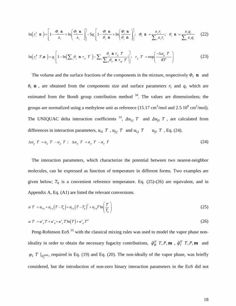
The volume and the surface fractions of the components in the mixture, respectively 𝛷𝛷𝑖𝑖(𝐧𝐧) and

𝜃𝜃𝑖𝑖(𝐧𝐧), are obtained from the components size and surface parameters 𝑟𝑟𝑖𝑖 and 𝑞𝑞𝑖𝑖 which are

estimated from the Bondi group contribution method 34. The values are dimensionless; the

groups are normalized using a methylene unit as reference (15.17 cm3/mol and 2.5⋅109 cm2/mol).

The UNIQUAC delta interaction coefficients 33, 𝛥𝛥𝑓𝑓𝑖𝑖𝑖𝑖(𝑇𝑇) and 𝛥𝛥𝑓𝑓𝑖𝑖𝑖𝑖(𝑇𝑇), are calculated from

differences in interaction parameters, 𝑓𝑓𝑖𝑖𝑖𝑖(𝑇𝑇), 𝑓𝑓𝑖𝑖𝑖𝑖(𝑇𝑇) and 𝑓𝑓𝑖𝑖𝑖𝑖(𝑇𝑇) = 𝑓𝑓𝑖𝑖𝑖𝑖(𝑇𝑇), Eq. (24).

( ) ( ) ( ); ( ) ( ) ( )ij ij jj ji ji iiu T u T u T u T u T u T∆ = − ∆ = − (24)

The interaction parameters, which characterize the potential between two nearest-neighbor

molecules, can be expressed as function of temperature in different forms. Two examples are

given below; 𝑇𝑇0 is a convenient reference temperature. Eq. (25)-(26) are equivalent, and in

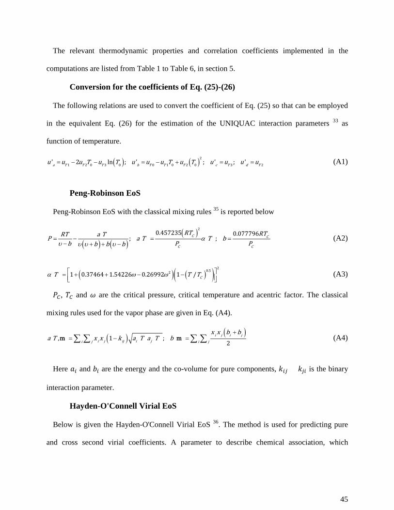
Appendix A, Eq. (A1) are listed the relevant conversions.

( ) ( )2

0 1 0 2 0 30

( ) lnT T T TTu T u u T T u T T u TT

= + − + − +

(25)

( ) 2( ) ' ' ' ln 'a b c du T u T u u T T u T= + + + (26)

Peng-Robinson EoS 35 with the classical mixing rules was used to model the vapor phase non-

ideality in order to obtain the necessary fugacity contributions, 𝜑𝜑�𝑔𝑔𝑉𝑉(𝑇𝑇,𝑑𝑑,𝐦𝐦), 𝜑𝜑�𝑖𝑖𝑉𝑉(𝑇𝑇,𝑑𝑑,𝐦𝐦) and

𝜑𝜑𝑖𝑖(𝑇𝑇)|𝑃𝑃𝑖𝑖𝑠𝑠𝑠𝑠𝑠𝑠, required in Eq. (19) and Eq. (20). The non-ideally of the vapor phase, was briefly

considered, but the introduction of non-zero binary interaction parameters in the EoS did not

18

have appreciable effect on the quality of the optimization. Peng-Robinson EoS 35 is reported in

Appendix A, Eq. (A2)-(A4).

The Hayden-O'Connell Virial EoS 36 was used in cases of systems containing acetic acid. The

method predicts the second Virial coefficient by using contributions which can account for the

polar and associating interactions, Appendix A, Eq. (A5)-(A24).

In all cases the most accurate gas phase model was used, without any tuning. Only binary

solubility data were used and only the UNIQUAC interaction parameters were fitted. In

principle, any gas phase model can be coupled with UNIQUAC, as long as the vapor phase is

correctly represented. The use of Hayden-O'Connell Virial EoS 36 for systems containing acetic

acid (rather than a cubic EoS) is owed to the fact that this component shows a monomer-dimer

equilibrium in the vapor phase, and this complex association behavior cannot be predicted by the

PR or Soave-Redlich-Kwong (SRK) EoS (in unmodified form). However, Hayden-O'Connell is

a Virial EoS truncated at the second coefficient, and this restricts its applicability to moderate

vapor densities only.

The saturation pressure for the pure solvent 𝑑𝑑𝑖𝑖𝑠𝑠𝑠𝑠𝑠𝑠 and the Henry’s law constant at the solvent

saturation pressure 𝐻𝐻𝑔𝑔(𝑇𝑇)�𝑃𝑃𝑖𝑖𝑠𝑠𝑠𝑠𝑠𝑠 are given respectively by Eq. (7) and Eq. (8) truncated at the third

term.

The volume of the solvent at saturation condition, 𝜐𝜐𝑖𝑖𝐿𝐿, is obtained from the DIPPR-105

Appendix A, Eq. (A25), and from DIPPR-116 Appendix A, Eq. (A26) for water 37.

The volume of the solute at infinite dilution �̅�𝜐𝑔𝑔∞ is taken from Brelvi and O’Connell correlation

38, Appendix A, Eq. (A27)-(A29); as for 𝜐𝜐𝑖𝑖𝐿𝐿, �̅�𝜐𝑔𝑔∞ it is assumed pressure independent.

19

4 Model parameter estimation

Experimental data were mainly taken from the original papers and from the IUPAC-NIST

solubility data series. An overview of the data used for the evaluation of model parameters and

relative references are given in the supporting information. Points at pressures above 400 bar and

temperatures above 90% of the solvent critical temperature were not included in the regressions.

Vapor compositions were not considered as well, they are available in only a few cases.

Low pressure constants, such as Bunsen coefficients, Ostwald coefficients and absorption

coefficients, were converted to mole fraction solubility. These units were originally obtained

applying ideal gas law, Raoult’s law and Henry’s law on the actual measured values; the same

assumptions were used to back-calculate mole fractions and total pressure. Occasionally

experimental points were given in graphic form only and they were then extracted from the

figures.

The only constants involved in the parameter fitting are ℎ1, ℎ2 and ℎ3 for the Henry’s law

constant at the saturation pressure of the solvent, Eq. (8); and 𝑓𝑓′𝑠𝑠 and 𝑓𝑓′𝑏𝑏 for the interaction

parameters of the UNIQUAC model, Eq. (26).

Unlike the Krichevsky-Ilinskaya and Krichevsky-Kasarnovsky approach, the volume of the

gas at infinite dilution is not a parameter involved in the regression; Instead the Brelvi and

O’Connell correlation 38, Appendix A, Eq. (A27)-(A29) is used to obtain �̅�𝜐𝑔𝑔∞ as function of

temperature. Inaccurate predictions of �̅�𝜐𝑔𝑔∞ may affect the quality of the fitting, particularly at

high pressures. Therefore data above 400 bar have not been included. Points at temperatures

above 90% of the solvent critical temperature were not considered either, since the simplified

form of the Poynting corrections becomes unreliable (close to 𝑇𝑇𝑖𝑖𝑔𝑔, the two liquid volumes, �̅�𝜐𝑔𝑔∞

and 𝜐𝜐𝑖𝑖𝐿𝐿, can no longer be considered incompressible).

20

UNIQUAC equation is often fitted to binary data in terms of delta interaction coefficients

(𝛥𝛥𝑓𝑓𝑖𝑖𝑖𝑖(𝑇𝑇) and 𝛥𝛥𝑓𝑓𝑖𝑖𝑖𝑖(𝑇𝑇)); and these, are the ones found in AspenTech software databanks 26 and in

the DECHEMA Chemistry Data Series 39. The 15 binary systems object of this study share

common components, therefore the independent estimation of the corresponding 15 coefficient

pairs would most likely produce model inconsistency; i.e. the coefficient pairs would not satisfy

closure equations such as [𝛥𝛥𝑓𝑓𝑖𝑖𝑘𝑘(𝑇𝑇) − 𝛥𝛥𝑓𝑓𝑘𝑘𝑖𝑖(𝑇𝑇)] = [𝛥𝛥𝑓𝑓𝑖𝑖𝑖𝑖(𝑇𝑇) − 𝛥𝛥𝑓𝑓𝑖𝑖𝑖𝑖(𝑇𝑇)] + [𝛥𝛥𝑓𝑓𝑖𝑖𝑘𝑘(𝑇𝑇) − 𝛥𝛥𝑓𝑓𝑘𝑘𝑖𝑖(𝑇𝑇)].

This equation, in conjunction with Eq. (24) , implies the invariance of the self-interaction

parameters 𝑓𝑓𝑖𝑖𝑖𝑖(𝑇𝑇), 𝑓𝑓𝑖𝑖𝑖𝑖(𝑇𝑇) and 𝑓𝑓𝑘𝑘𝑘𝑘(𝑇𝑇).

To ensure model consistency, the regression was performed in terms of interaction parameters

(𝑓𝑓𝑖𝑖𝑖𝑖(𝑇𝑇), 𝑓𝑓𝑖𝑖𝑖𝑖(𝑇𝑇) and 𝑓𝑓𝑖𝑖𝑖𝑖(𝑇𝑇) = 𝑓𝑓𝑖𝑖𝑖𝑖(𝑇𝑇)); which reduces the number of parameter required from 30

to 22. From 15 Δ𝑓𝑓𝑔𝑔𝑖𝑖 and 15 Δ𝑓𝑓𝑖𝑖𝑔𝑔 (delta interaction coefficients pairs) down to 15 𝑓𝑓𝑔𝑔𝑖𝑖 = 𝑓𝑓𝑔𝑔𝑖𝑖 (gas-

solvent interaction parameters), 5 𝑓𝑓𝑔𝑔𝑔𝑔 (gas-gas self-interaction parameters), and 3 𝑓𝑓𝑖𝑖𝑖𝑖 (solvent-

solvent self-interaction parameters). The H2O-H2O self-interaction parameter was set to zero as

done in Thomsen et al. 40. This influences the numerical value for the remaining terms, but not

the value of the delta interaction coefficients, as they are calculated as differences, Eq. (24).

The use of a reduced set of parameters has also the advantage of narrowing the confidence

interval and reducing the risk of an over-parametrized model (less ambiguity on the delta

interaction coefficients). Small losses in fitting accuracy are to be expected.

The evaluation of the constants which determine the temperature dependence of the Henry’s

law constant at the saturation pressure of the solvent and the UNIQUAC interaction parameters,

respectively Eq. (8) and Eq. (26), was executed with Levenberg-Marquardt algorithm by

minimization of the objective function reported in Eq. (27)-(29). All experimental points

producing deviations higher than a certain threshold were not included in the final regression.

21

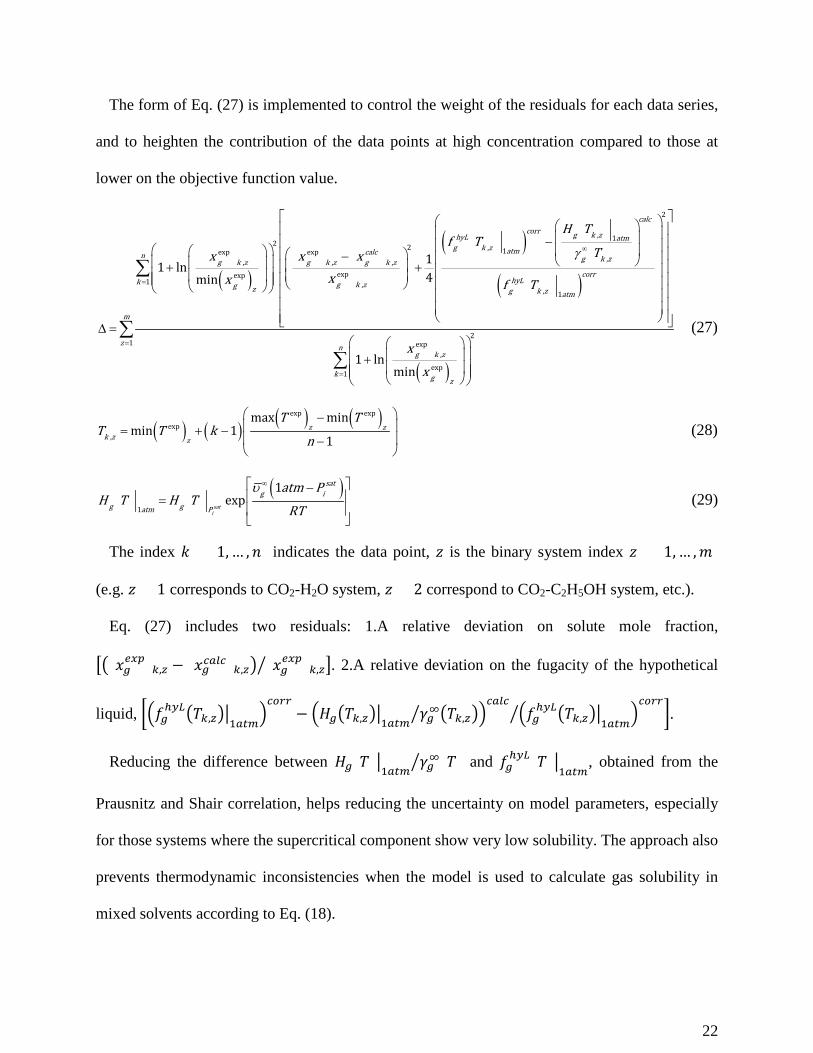
The form of Eq. (27) is implemented to control the weight of the residuals for each data series,

and to heighten the contribution of the data points at high concentration compared to those at

lower on the objective function value.

( )

( )

( )

2

, 12 2 , 1exp exp

,, , ,expexp

,, 1

( )( )

( )( ) ( ) ( ) 11 ln4( )min ( )

calccorr g k zhyL atm

g k z atmcalcg k zg k z g k z g k zcorr

hyLk g k zg z g k z atm

H Tf T

Tx x xxx f T

γ ∞

− − + +

∆ =

( )

1

21 exp

,

exp1

( )1 ln

min

n

m

z ng k z

k g z

x

x

=

=

=

+

∑

∑

∑

(27)

( ) ( ) ( ) ( )exp exp

exp,

max minmin 1

1z z

k z z

T TT T k

n

− = + − −

(28)

( )1

1( ) ( ) exp

sati

satg i

g gatm P

atm PH T H T

RTυ ∞ − =

(29)

The index 𝑘𝑘 = [1, … ,𝑓𝑓] indicates the data point, 𝑧𝑧 is the binary system index 𝑧𝑧 = [1, … ,𝑚𝑚]

(e.g. 𝑧𝑧 = 1 corresponds to CO2-H2O system, 𝑧𝑧 = 2 correspond to CO2-C2H5OH system, etc.).

Eq. (27) includes two residuals: 1.A relative deviation on solute mole fraction,

��(𝑥𝑥𝑔𝑔𝑒𝑒𝑒𝑒𝑒𝑒)𝑘𝑘,𝑧𝑧 − (𝑥𝑥𝑔𝑔𝑐𝑐𝑠𝑠𝑠𝑠𝑐𝑐)𝑘𝑘,𝑧𝑧� (𝑥𝑥𝑔𝑔

𝑒𝑒𝑒𝑒𝑒𝑒)𝑘𝑘,𝑧𝑧� �. 2.A relative deviation on the fugacity of the hypothetical

liquid, ��𝑓𝑓𝑔𝑔ℎ𝑦𝑦𝐿𝐿�𝑇𝑇𝑘𝑘,𝑧𝑧��1𝑠𝑠𝑠𝑠𝑎𝑎�

𝑐𝑐𝑠𝑠𝑐𝑐𝑐𝑐− �𝐻𝐻𝑔𝑔�𝑇𝑇𝑘𝑘,𝑧𝑧��1𝑠𝑠𝑠𝑠𝑎𝑎 𝛾𝛾𝑔𝑔∞�𝑇𝑇𝑘𝑘,𝑧𝑧�� �

𝑐𝑐𝑠𝑠𝑠𝑠𝑐𝑐�𝑓𝑓𝑔𝑔

ℎ𝑦𝑦𝐿𝐿�𝑇𝑇𝑘𝑘,𝑧𝑧��1𝑠𝑠𝑠𝑠𝑎𝑎�𝑐𝑐𝑠𝑠𝑐𝑐𝑐𝑐

� �.

Reducing the difference between 𝐻𝐻𝑔𝑔(𝑇𝑇)�1𝑠𝑠𝑠𝑠𝑎𝑎

𝛾𝛾𝑔𝑔∞(𝑇𝑇)� and 𝑓𝑓𝑔𝑔ℎ𝑦𝑦𝐿𝐿(𝑇𝑇)�

1𝑠𝑠𝑠𝑠𝑎𝑎, obtained from the

Prausnitz and Shair correlation, helps reducing the uncertainty on model parameters, especially

for those systems where the supercritical component show very low solubility. The approach also

prevents thermodynamic inconsistencies when the model is used to calculate gas solubility in

mixed solvents according to Eq. (18).

22

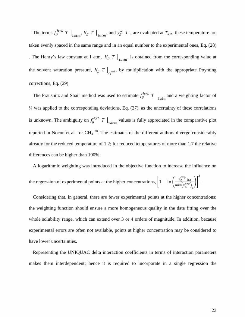
The terms 𝑓𝑓𝑔𝑔ℎ𝑦𝑦𝐿𝐿(𝑇𝑇)�

1𝑠𝑠𝑠𝑠𝑎𝑎, 𝐻𝐻𝑔𝑔(𝑇𝑇)�

1𝑠𝑠𝑠𝑠𝑎𝑎, and 𝛾𝛾𝑔𝑔∞(𝑇𝑇), are evaluated at 𝑇𝑇𝑘𝑘,𝑧𝑧, these temperature are

taken evenly spaced in the same range and in an equal number to the experimental ones, Eq. (28)

. The Henry’s law constant at 1 atm, 𝐻𝐻𝑔𝑔(𝑇𝑇)�1𝑠𝑠𝑠𝑠𝑎𝑎

, is obtained from the corresponding value at

the solvent saturation pressure, 𝐻𝐻𝑔𝑔(𝑇𝑇)�𝑃𝑃𝑖𝑖𝑠𝑠𝑠𝑠𝑠𝑠 , by multiplication with the appropriate Poynting

corrections, Eq. (29).

The Prausnitz and Shair method was used to estimate 𝑓𝑓𝑔𝑔ℎ𝑦𝑦𝐿𝐿(𝑇𝑇)�

1𝑠𝑠𝑠𝑠𝑎𝑎and a weighting factor of

¼ was applied to the corresponding deviations, Eq. (27), as the uncertainty of these correlations

is unknown. The ambiguity on 𝑓𝑓𝑔𝑔ℎ𝑦𝑦𝐿𝐿(𝑇𝑇)�

1𝑠𝑠𝑠𝑠𝑎𝑎 values is fully appreciated in the comparative plot

reported in Nocon et al. for CH4 28. The estimates of the different authors diverge considerably

already for the reduced temperature of 1.2; for reduced temperatures of more than 1.7 the relative

differences can be higher than 100%.

A logarithmic weighting was introduced in the objective function to increase the influence on

the regression of experimental points at the higher concentrations, �1 + ln�(xgexp)k,z

min�xgexp�

z

��2

.

Considering that, in general, there are fewer experimental points at the higher concentrations;

the weighting function should ensure a more homogeneous quality in the data fitting over the

whole solubility range, which can extend over 3 or 4 orders of magnitude. In addition, because

experimental errors are often not available, points at higher concentration may be considered to

have lower uncertainties.

Representing the UNIQUAC delta interaction coefficients in terms of interaction parameters

makes them interdependent; hence it is required to incorporate in a single regression the

23

experimental points relevant to all 15 systems. Each contribution is normalized using the

summation of the weights.

The numbers of points involved in the model parameter estimation are given in table format as

supporting information.

5 Modelling results

The parameter values, obtained as solution of the minimization problem, Eq. (27), are reported

in Table 1. The first two columns list the constants, 𝑓𝑓𝑇𝑇0 and 𝑓𝑓𝑇𝑇1, for the temperature dependent

UNIQUAC interaction parameters, Eq. (25), both for unlike and self-interactions.

The values reported in Table 1 for 𝑓𝑓𝑇𝑇0 and 𝑓𝑓𝑇𝑇1 are not limited to the particular EoS that has

been implemented in the parametrization procedure. In principle, UNIQUAC equation, with the

adoption of these constants, can be used in combination with any gas phase model, provided the

vapor phase is correctly represented by the EoS chosen.

The regression of the UNIQUAC model in terms of interaction parameters, rather than delta

interaction coefficients, has the advantage of exposing trends that otherwise would not be

evident. For instance, it can be seen that, for the same supercritical component, 𝑓𝑓𝑇𝑇1 is, in all

cases, smaller in magnitude for the systems containing water, and larger for the systems

containing ethanol as solvent. It can also be observed that 𝑓𝑓𝑇𝑇0 has similar values for systems of

the same gas in ethanol and in acetic acid, but a very different value for systems where the

solvent is water.

In Table 1, from the third to fifth column, are listed the coefficients for the temperature

dependent Henry’s law constant, Eq. (8). For CH4-CH3COOH system the available experimental

points cover a rather small temperature range, from 298 to 348 K, thus only two coefficients

were subjected to parametrization.

24

The last two columns report the Absolute average deviations (AAD%) for 𝑥𝑥𝑔𝑔 and

𝑓𝑓𝑔𝑔ℎ𝑦𝑦𝐿𝐿(𝑇𝑇)�

1𝑠𝑠𝑠𝑠𝑎𝑎, respectively calculated as 1 𝑓𝑓⁄ ∑ ��(𝑥𝑥𝑔𝑔

𝑒𝑒𝑒𝑒𝑒𝑒)𝑘𝑘 − (𝑥𝑥𝑔𝑔𝑐𝑐𝑠𝑠𝑠𝑠𝑐𝑐)𝑘𝑘� (𝑥𝑥𝑔𝑔𝑒𝑒𝑒𝑒𝑒𝑒)𝑘𝑘� �𝑛𝑛

𝑘𝑘=1 ,

1 𝑓𝑓⁄ ∑ ��𝑓𝑓𝑔𝑔ℎ𝑦𝑦𝐿𝐿(𝑇𝑇𝑘𝑘)�

1𝑠𝑠𝑠𝑠𝑎𝑎�𝑐𝑐𝑠𝑠𝑐𝑐𝑐𝑐

− �𝐻𝐻𝑔𝑔(𝑇𝑇𝑘𝑘)�1𝑠𝑠𝑠𝑠𝑎𝑎

𝛾𝛾𝑔𝑔∞(𝑇𝑇𝑘𝑘)� �𝑐𝑐𝑠𝑠𝑠𝑠𝑐𝑐

�𝑓𝑓𝑔𝑔ℎ𝑦𝑦𝐿𝐿(𝑇𝑇𝑘𝑘)�

1𝑠𝑠𝑠𝑠𝑎𝑎�𝑐𝑐𝑠𝑠𝑐𝑐𝑐𝑐

� �𝑛𝑛𝑘𝑘=1 , the

𝑓𝑓𝑔𝑔ℎ𝑦𝑦𝐿𝐿(𝑇𝑇𝑘𝑘)�

1𝑠𝑠𝑠𝑠𝑎𝑎 values are the ones from Prausnitz and Shair correlation.

Table 1: Temperature dependent constants for UNIQUAC interaction parameters 33, Eq. (25).Temperature dependent parameters for Henry’s law constant, Eq. (8); the equation gives the Henry’s law constant at solvent saturation pressure in bar when the temperature is expressed in K. Temperature and pressure range of the data points involved in the regression. Absolute average deviations, (AAD%), for 𝑥𝑥𝑔𝑔 and 𝑓𝑓𝑔𝑔

ℎ𝑦𝑦𝐿𝐿(𝑇𝑇)�1𝑠𝑠𝑠𝑠𝑎𝑎

For the solubilities of H2 in CH3COOH above 1 atm the only study available is Jónasson at all

41. The experimental points from this source are, however, not in agreement with the datasets at

atmospheric pressure listed in the two other sources found: Maxted and Moon 42 and Just 43. Due

to the impossibility to confirm the exactness of Jónasson at all results, the system H2-CH3COOH

𝑓𝑓𝑇𝑇0 [J mol-1]

𝑓𝑓𝑇𝑇1 [J mol-1K-1] ℎ1 ℎ2 ℎ3

Datasets range AAD [%] 𝑇𝑇 [K] 𝑑𝑑[bar] 𝑥𝑥𝑔𝑔 𝑓𝑓𝑔𝑔

ℎ𝑦𝑦𝐿𝐿(𝑇𝑇)�1𝑠𝑠𝑠𝑠𝑎𝑎

CO2-H2O 9213 -43.50 134.66 -7519.4 -17.883 273-582 0.13-365 7.4 7.5 CO2-C2H5OH 7227 -74.65 70.28 -3121.6 -9.611 283-423 0.85-145 12.6 5.1 CO2-CH3COOH 7215 -51.23 30.84 -2481.6 -3.147 283-365 1.01-111 3.1 6.8 CO-H2O 21197 -87.22 139.39 -6631.6 -18.628 273-498 0.48-138 5.9 11.2 CO-C2H5OH 13635 -97.33 34.80 -1108.2 -4.133 293-448 1.01-83 7.3 6.3 CO-CH3COOH 14482 -90.00 24.82 -740.2 -2.538 293-448 1.01-70 3.9 6.2 CH4-H2O 11285 -52.45 151.45 -7452.3 -20.329 273-573 0.58-367 5.8 9.6 CH4-C2H5OH 6549 -79.57 151.77 -6600.5 -21.544 280-398 1.01-314 10.1 6.0 CH4-CH3COOH 7787 -64.96 8.15 -197.4 — 298-348 2.60-70 2.9 0.8 N2-H2O 13722 -37.58 116.32 -5642.9 -15.095 273-433 1.01-305 7.9 10.1 N2-C2H5OH 8283 -69.85 66.85 -2642.1 -8.783 233-398 0.85-99 3.7 3.9 N2-CH3COOH 9592 -67.97 50.73 -1725.4 -6.398 293-473 1.01-61 7.9 0.7 H2-H2O 12631 -45.95 85.99 -3593.0 -11.019 273-575 1.01-405 4.9 9.8 H2-C2H5OH 6621 -66.31 86.26 -3412.2 -11.646 273-448 1.01-317 5.2 4.5 H2-CH3COOH — — — — — — — — — CO2-CO2 5794 -59.07 CO-CO 11468 -113.35 CH4-CH4 3055 -81.08 N2-N2 3799 -87.96 H2-H2 2731 -91.34 H2O-H2O a0 a0 C2H5OH-C2H5OH 5414 -54.15 CH3COOH-CH3COOH 6968 -53.90 aH2O-H2O interaction is set to 0, as explained in section 4

25

was not included in the data regression. For reference purposes, the relevant literature

information are reported in Table 15 in the supporting information.

Table 2: Pure component parameters for Peng-Robinson EoS 35, Appendix A, Eq. (A2)-(A4), and Hayden-O'Connell Virial EoS 36, Appendix A, Eq. (A5)-(A24)

Table 2 reports the pure component parameters adopted in Peng-Robinson EoS and Hayden-

O'Connell Virial EoS for the modeling of the vapor phase. The mean radius of gyrations, 𝑟𝑟𝑔𝑔𝑖𝑖𝑐𝑐,

are obtained from the molecular moments of inertia and the molecular masses as described in

Hayden and O'Connell paper.

Table 3: Association parameters for pure interactions, 𝜂𝜂𝑖𝑖𝑖𝑖, and solvation parameter for unlike interactions, 𝜂𝜂𝑖𝑖𝑖𝑖, for Hayden-O'Connell Virial EoS 36, Appendix A, Eq. (A5)-(A24)

Table 3 lists the relevant values for 𝜂𝜂𝑖𝑖𝑖𝑖 and 𝜂𝜂𝑖𝑖𝑖𝑖, from 44. Since the association parameters, 𝜂𝜂𝑖𝑖𝑖𝑖,

for acetic the acid is equal to 4.5, the equilibrium constant of the dimerization reaction is here

given as well; indeed the second Virial coefficient for this interaction, is calculated according to

the chemical theory of dimerization, Appendix A, Eq. (A24).

Table 4 reports volumes and surface area parameters used in the UNIQUAC model; those

constants are dimensionless. For water, 𝑟𝑟 and 𝑞𝑞 values, were those assigned by Abrams and

CO2 CO CH4 N2 H2 H2O C2H5OH CH3COOH 𝑇𝑇𝑔𝑔 [K] 304.2 132.9 190.6 126.2 33.2 647.1 514.0 591.9 𝑑𝑑𝑔𝑔 [bar] 73.8 35.0 46.00 34.0 13.1 220.6 61.4 57.9 𝜔𝜔 0.2236 0.0482 0.0115 0.0377 -0.2160 0.3449 0.6436 — 𝑟𝑟𝑔𝑔𝑖𝑖𝑐𝑐 [m] 1.04⋅10-10 5.58⋅10-11 1.12⋅10-10 5.47⋅10-11 — — — 2.61⋅10-10 𝜇𝜇 [D] 0 0.1121 0 0 — — — 1.7388

𝜂𝜂𝑖𝑖𝑖𝑖/𝜂𝜂𝑖𝑖𝑖𝑖 CH3COOH CO2 CO CH4 N2 CH3COOH a4.5 0.5 0 0 0 CO2 — 0.16 0 0 0 CO — — 0 0 0 CH4 — — — 0 0 N2 — — — — 0 aThe equilibrium constant for acetic acid association reaction as function of temperature is 𝐾𝐾𝑖𝑖𝑖𝑖(𝑇𝑇) = 𝑒𝑒𝑥𝑥𝑒𝑒(7290/𝑇𝑇 − 17.36)

26

Prausnitz 33; while, for the remaining molecules, the values were obtained from the Bondi

contribution method 34.

Table 4: Pure component parameters, 𝑟𝑟 and 𝑞𝑞 for UNIQUAC model 33 from Bondi contribution method 34, Eq (21)-(23). Characteristic volumes for Brelvi-O’Connell correlation 38, Appendix A, Eq. (A27)-(A29)

Initially, for the two systems H2-H2O and H2-C2H5OH, it was not possible to simultaneously

fit, within an acceptable tolerance, both solubility data and fugacity of hypothetical liquid H2 at 1

atm (as obtained from Prausnitz and Shair correlation). Indeed, it was found that the value of

1.20 Å, assigned by Bondi 34 to the Van der Waals radius of hydrogen atoms and typically used

to calculate 𝑟𝑟 and 𝑞𝑞 for organic molecules, was not appropriate for the estimation of 𝑟𝑟 and 𝑞𝑞 in

H2 molecule. A larger radius appeared to be the only way to obtain satisfactory results.

The Batsanov study on the hydrogen radii in different gas phase and condensed molecules 45

certainly indicates the great variability in dimensions of this element in relation to the

electronegativity of the atom at which is directly bonded. This might be explained considering

that hydrogen has only one occupied orbital and only one electron; the extent of the

delocalization of this single electron, when involved in the formation of a covalent bond,

strongly affects the size of the electron cloud around the hydrogen nucleus.

Based on this evidence, the 𝑟𝑟 and 𝑞𝑞 parameters listed in Table 4, in bold, were calculated using

a Van der Waals radius of 1.52 Å, as reported for hydrogen atoms specifically for H2 molecule in

the Batsanov study 45. Whit the new coefficients, was possible to reduce the AAD% on the

fugacity of hypothetical liquid H2 at 1 atm pressure to the final values reported in Table 1, in

bold.

CO2 CO CH4 N2 H2 H2O C2H5OH CH3COOH 𝑞𝑞 1.292 1.112 1.152 1.088 0.870 1.400 1.972 2.072 𝑟𝑟 1.2986 1.0679 1.1239 1.0415 0.7940 0.9200 2.1056 2.1951 𝜐𝜐′𝑔𝑔 [cm3/mol] 94.0 94.4 98.6 89.2 64.15 46.32 157.58 155.94

27

In Table 4 are also listed the characteristic volumes, 𝜐𝜐′𝑔𝑔, used in Brelvi-O’Connell correlation

for estimating �̅�𝜐𝑔𝑔∞ in the different solvents, Appendix A, Eq. (A27)-(A29). For all gases, 𝜐𝜐′𝑔𝑔 was

considered equal to the critical volume of the substance, since, for nonpolar species, 𝜐𝜐′𝑔𝑔/𝜐𝜐𝑔𝑔 ≅ 1,

38. For polar substances, such as water, acetic acid and ethanol, 𝜐𝜐′𝑔𝑔 tend to be smaller than 𝜐𝜐𝑔𝑔 and

the assumption 𝜐𝜐′𝑔𝑔/𝜐𝜐𝑔𝑔 ≅ 1 can no longer be considered correct, especially when 𝜐𝜐𝑔𝑔 is that of the

solvent (e.g. for water, the use of critical volume, in place of the characteristic volume, can lead

to underestimations of �̅�𝜐𝑔𝑔∞ as large as 50%). The value reported in Table 4 for water is the one

assigned by Brelvi and O’Connell 38. For ethanol, 𝜐𝜐′𝑔𝑔 was determined by fitting Appendix A, Eq.

(A29) to the density and to the isothermal compressibility data reported in 46 and 47; and for

acetic acid was obtained by fitting Appendix A, Eq. (A1) only to the isothermal density datasets

reported in 48.

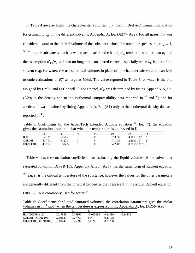
Table 5: Coefficients for the AspenTech extended Antoine equation 26, Eq. (7); the equation gives the saturation pressure in bar when the temperature is expressed in K

Table 6 lists the correlation coefficients for estimating the liquid volumes of the solvents at

saturated condition. DIPPR-105, Appendix A, Eq. (A25), has the same form of Rackett equation

49, e.g. 𝑙𝑙3 is the critical temperature of the substance, however the values for the other parameters

are generally different from the physical properties they represent in the actual Rackett equation.

DIPPR-116 is commonly used for water 37.

Table 6: Coefficients for liquid saturated volumes, the correlation parameters give the molar volumes in cm3 mol-1 when the temperature is expressed in K, Appendix A, Eq. (A25)-(A26)

𝑒𝑒1 𝑒𝑒2 𝑒𝑒3 𝑒𝑒4 𝑒𝑒5 𝑒𝑒6 𝑒𝑒7 H2O 62.1361 -7258.2 0 0 -7.3037 4.1653⋅10-6 2 C2H5OH 61.7911 -7122.3 0 0 -7.1424 2.8853⋅10-6 2 CH3COOH 41.7571 -6304.5 0 0 -4.2985 8.8865⋅10-18 6

𝑙𝑙1 𝑙𝑙2 𝑙𝑙3 𝑙𝑙4 𝑙𝑙5 H2O (DIPPR-116) 0.017863 0.05860 -0.095396 0.21389 -0.14126 C2H5OH (DIPPR-105) 0.001629 0.27469 514 0.23178 CH3COOH (DIPPR-105) 0.001448 0.25892 591.95 0.25290

28

6 Discussion

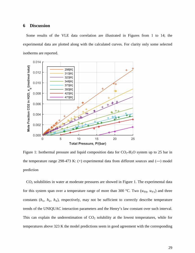
Some results of the VLE data correlation are illustrated in Figures from 1 to 14; the

experimental data are plotted along with the calculated curves. For clarity only some selected

isotherms are reported.

Figure 1: Isothermal pressure and liquid composition data for CO2-H2O system up to 25 bar in

the temperature range 298-473 K: (+) experimental data from different sources and (―) model

prediction

CO2 solubilities in water at moderate pressures are showed in Figure 1. The experimental data

for this system span over a temperature range of more than 300 °C. Two (𝑓𝑓𝑇𝑇0, 𝑓𝑓𝑇𝑇1) and three

constants (ℎ1, ℎ2, ℎ3), respectively, may not be sufficient to correctly describe temperature

trends of the UNIQUAC interaction parameters and the Henry’s law constant over such interval.

This can explain the underestimation of CO2 solubility at the lowest temperatures, while for

temperatures above 323 K the model predictions seem in good agreement with the corresponding

29

experimental points. Indeed, in approximately the same temperature range the vapor pressures of

pure water are commonly fitted using 5 coefficients (e.g. the non-zero coefficients reported in

Table 5 for the AspenTech extended Antoine equation 26, or the 5 coefficients adopted for water

in DIPPR-101 equation 37).

Figure 2: Isothermal pressure and liquid composition data for CO2-H2O system up to 220 bar in

the temperature range 293-333 K: (+) experimental data from different sources and (―) model

prediction

CO2 solubilities in water for pressure up to 220 bar and temperature up to 333 K are reported

in Figure 2. The two isotherms at 293 K and 298 K were plotted only for pressures below the

liquid-liquid split (50, 51, 52). This is done because the model parameters are not intended, and

should not be used to represents VLLE or LLE regions, in view of the fact, at these conditions,

the second phase (the CO2 rich liquid) is too close to its critical point, and the assumption of

pressure independent liquid volumes is not any more realistic. It is still noteworthy that, even if

30

no LLE or VLLE data were involved in the parametrization, the coefficients reported in Table 4

for this system, allow for the model to approximatively predict the pressures at which the liquid-

liquid split occurs and, though only qualitatively, to predict the CO2 rich liquid phase

compositions. For all isotherms at pressures below 80 bar, the deviations between the model

predictions and the experimental points are mainly due to the scatter in the data. For higher

pressure CO2 solubilities are generally over-predicted, but also the experimental points from the

different sources differ quite remarkably from each other, e.g. the points at 313 K between 40

and 100 bar, primarily from 53 and 54.

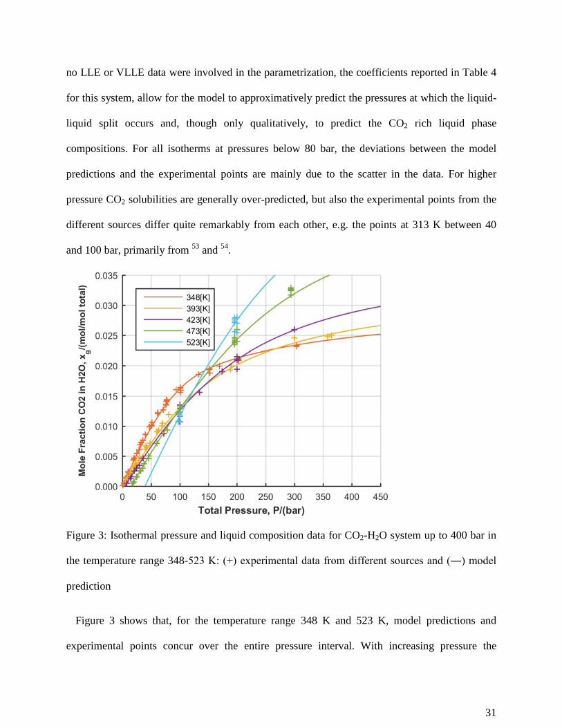
Figure 3: Isothermal pressure and liquid composition data for CO2-H2O system up to 400 bar in

the temperature range 348-523 K: (+) experimental data from different sources and (―) model

prediction

Figure 3 shows that, for the temperature range 348 K and 523 K, model predictions and

experimental points concur over the entire pressure interval. With increasing pressure the

31

Poynting correction tends to diminish the gas solubility compared to a straight line prediction,

however the reason of the sharp change in the slope of the isotherms observed in Figures 2 and 3

at around 80-100 bar is due to a strong non ideality of CO2 in the vapor phase. Though

supercritical above 305 K, for the higher pressures considered in the present study, pure CO2 can

still show liquid-like densities and sharp variations in the compressibility factor. The model

prediction for the system CO2-H2O agrees well with the experimental data within the

temperatures and pressures range of the datasets involved in the regression, Table 1.

Figure 4: Isothermal pressure and liquid composition data for CO2-C2H5OH system up to 70 bar

in the temperature range 283-308 K: (+) experimental data from different sources and (―) model

prediction

32

Figure 5: Isothermal pressure and liquid composition data for CO2-C2H5OH system up to 120 bar

in the temperature range 313-373 K: (+) experimental data from different sources and (―) model

prediction

CO2 solubilities in ethanol, for pressure up to 70 bar and temperature from 283 to 308 K, are

reported in Figure 4. Below 283 K, the model can be used to calculate the phase equilibrium over

the entire compositional range. For the other isotherms the critical conditions are progressly

reached for smaller amounts of CO2 in the mixture; that's the reason the lines in Figures 4 and 5

are not extend beyond a certain CO2 concertation. CO2-C2H5OH is also the system that shows the

lager deviation between model predictions and experimental data, as can be seen from the

corresponding AAD% value of 12.6% repotted in Table 1. Figures 4 and 5 give an insight on the

possible causes. The scatter of the experimental points around the corresponding isotherms is

evidently the main reason for the high AAD%. Another explanation could be that data too close

to the mixture critical conditions were used and therefore not properly modelled in the 𝛾𝛾 − 𝜑𝜑

33

framework. This is especially seen in the two isotherms at 298 K and 308 K, Figure 4, above 50

bar, where the model seems to indicate a slightly more straight behavior compared to the more

concave trend in the data. Within the boundary imposed by the mixture critical conditions and

the temperature and pressure ranges reported in Table 1, and despite the poor quality of the data,

the behavior of the system CO2-C2H5OH is adequately reproduced by the model.

Figure 6: Isothermal pressure and liquid composition data for CO-H2O system up to 140 bar in

the temperature range 298-498 K: (+) experimental data from different sources and (―) model

prediction

CO-H2O is a reactive system, as the water gas shift reaction (WGS) is thermodynamically

favorable. According to Jung and Knacke study 55, for temperature above 250 °C the reaction

turnover is sufficiently high to affect the chemical composition of the system, even in the

absence of an appropriate catalyst. For this reason, CO solubility measurements, conducted at

temperatures above 520 K, were not included in the data regression. Figure 6 reports the

34

isotherms and the experimental points for CO-H2O system in the temperature range 298 K to 498

K and pressures up 140 bar. All isotherms show a linear trend, as to be expected from systems of

sparingly soluble gases, but at the higher pressures, a slight positive curvature should still be

present. This is not the case since the growth of the Pointing term is somehow balanced by a

decrease in the solute activity coefficient; i.e. 𝛾𝛾𝑔𝑔∗(𝑇𝑇,𝐧𝐧) exp��̅�𝜐𝑔𝑔∞(𝑑𝑑 − 𝑑𝑑𝑖𝑖𝑠𝑠𝑠𝑠𝑠𝑠)/𝑅𝑅𝑇𝑇� ≅ 1. The model

correctly predicts the experimental data over the entire range, Table 1.

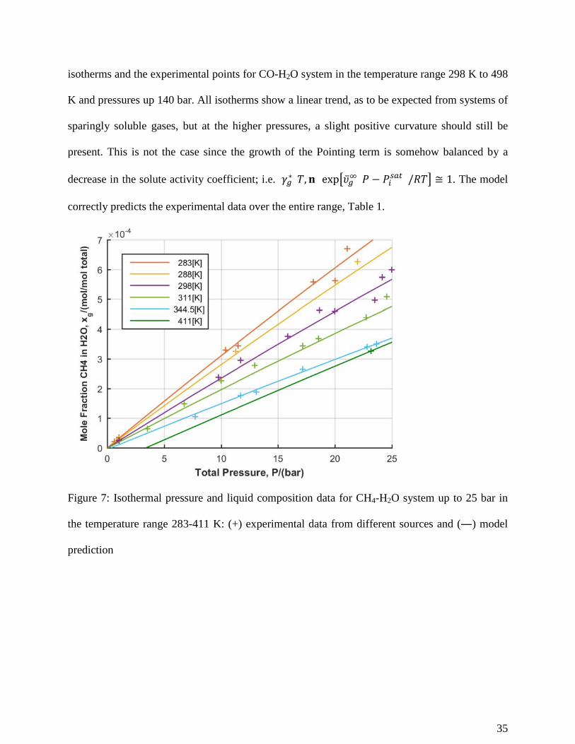
Figure 7: Isothermal pressure and liquid composition data for CH4-H2O system up to 25 bar in

the temperature range 283-411 K: (+) experimental data from different sources and (―) model

prediction

35

Figure 8: Isothermal pressure and liquid composition data for CH4-H2O system up to 350 bar in

the temperature range 278-411 K: (+) experimental data from different sources and (―) model

prediction

Figures 7 and 8 and, shows the solubilities of CH4 in water for two ranges of pressure,

respectively up to 25 bar and up to 350 bar. At high pressures and for temperatures below 20 °C,

the formation of CH4-H2O clathrate crystals may lead to incorrect estimations of CH4 solubility

56; thus points presenting unusually high CH4 solubilities, clearly non in line with the rest of the

experimental data, were discarded in advance. The model correctly predicts the mole fraction of

CH4 in water for the entire range of pressure considered in Figure 7, and for the first half of the

pressure interval reported in Figure 8. Above 200 bar, gas solubilities seems to be overestimated

in particular for the isotherms at 311 K and 344.5 K. Model predictions are consistent with the

trends of the datasets even in the vicinity of the experimental data; e.g. for the isotherms at 553 K

and 565 K up to 350 bar.

36

Figure 9: Isothermal pressure and liquid composition data for CH4-C2H5OH system up to 350 bar

in the temperature range 280-398 K: (+) experimental data from different sources and (―) model

prediction

CH4-C2H5OH, in Figure 9, is the system that shows the second larger deviations between

experimental points and model predictions, however, the various datasets from the different

sources are not always in agreement to each other. This can be appreciated from the isotherm at

298 K, the only sources available for pressures above atmospheric are 57 and 58, in the range

common to the two studies (up to 120 bar), the first datasets suggests higher solubilities, while

the second one shows lower solubilities than the calculated ones. The general trend of the

experimental points implies a linear dependence of CH4 solubilities from pressure; while, the

isotherms at 348 K and 398 K, show a clear reduction in CH4 solubilities due to a consistent

growth of the Pointing term at higher temperatures. The isotherm at 398 K cannot be extended

further, since for higher CH4 content in the liquid, the mixture closely approaches its critical

37

conditions, 57. For the highest pressure considered in Figure 9, the model predictions show a

behavior opposite to that indicated by the experimental points and more similar to that of CO2-

C2H5OH system. Aside from the datasets quality, this could be due to an overestimation in the

molar volume of CH4 in this solvent, leading to a compensating effect at the expense of the

UNIQUAC parameters. In fact, the type of behavior observed in Figure 9 is mainly related to the

Poynting correction and the applied molar volumes, since the UNIQUAC model was used

without any tuning of �̅�𝜐𝑔𝑔∞. Acceptable prediction can still be obtained for temperatures between

290 K and 350 K up to 300 bar.

Figure 10: Isothermal pressure and liquid composition data for N2-H2O system up to 30 bar in the

temperature range 274-413 K: (+) experimental data from different sources and (―) model

prediction

38

Figure 11: Isothermal pressure and liquid composition data for N2-H2O system up to 350 bar in

the temperature range 274-433 K: (+) experimental data from different sources and (―) model

prediction

Figures 10 and 11 shows the solubilities of N2 in water for two ranges of pressure, respectively

up to 30 bar and up to 350 bar. Model prediction and experimental points seems in good

agreement, both suggest a linear relationship between solubility and pressure over the entire

temperature interval considered, Table 1. As previously observed for CO-H2O system, Figure 6,

this is the result of the balancing of two competing contributions to the fugacity of the solute: the

pressure effect on the chemical potential, represented by the Pointing term, and the non-ideality

of the solution, accounted by the activity coefficient.

39

Figure 12: Isothermal pressure and liquid composition data for H2-H2O system up to 100 bar in

the temperature range 273-533 K: (+) experimental data from different sources and (―) model

prediction

Similarly to CO and N2 in water, the system H2-H2O, in Figures 12 and 13, shows linear

dependency of H2 solubilities from pressure, and for the isotherms below 373 K this behavior is

maintained up to 450 bar. Though H2 has the smallest partial molar volume among the gas

considered in this study, the Pointing term should visibly affect the curvature of the isotherms, in

a sense of reducing the solubilities compared to a straight line prediction, at least for the highest

pressures. The fact that the calculated isotherms and the experimental points lie on straight lines,

is evidence of a small deviation from the ideal diluted solution behavior even for H2 concertation

less than 0.01 mole fraction. It should however be considered that for the higher pressures

reported in Figure 13 also the fugacity coefficient for H2 in the vapor phase deviate noticeably

from 1. This is especially true, regardless of pressure, for the isotherm at 575 K. For this system,

40

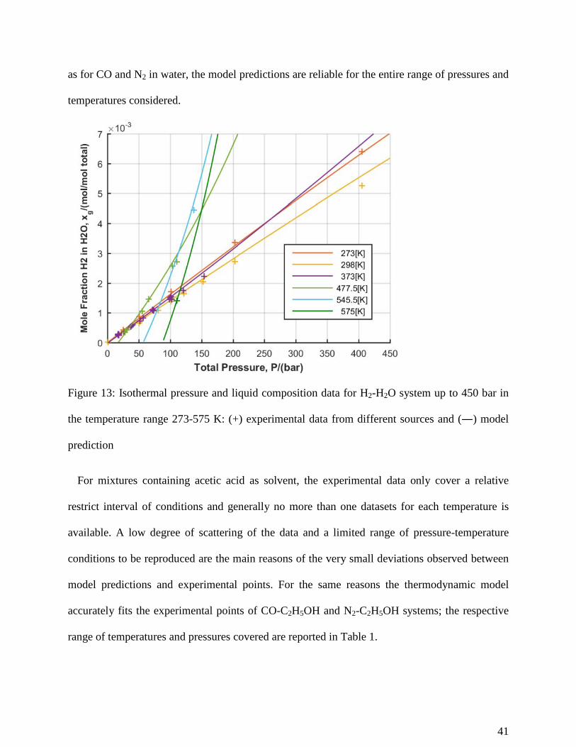
as for CO and N2 in water, the model predictions are reliable for the entire range of pressures and

temperatures considered.

Figure 13: Isothermal pressure and liquid composition data for H2-H2O system up to 450 bar in

the temperature range 273-575 K: (+) experimental data from different sources and (―) model

prediction

For mixtures containing acetic acid as solvent, the experimental data only cover a relative

restrict interval of conditions and generally no more than one datasets for each temperature is

available. A low degree of scattering of the data and a limited range of pressure-temperature

conditions to be reproduced are the main reasons of the very small deviations observed between

model predictions and experimental points. For the same reasons the thermodynamic model

accurately fits the experimental points of CO-C2H5OH and N2-C2H5OH systems; the respective

range of temperatures and pressures covered are reported in Table 1.

41

Figure 14: Isothermal pressure and liquid composition data for H2-C2H5OH system up to 350 bar

in the temperature range 298-448 K: (+) experimental data from different sources and (―) model

prediction

Figure 14 shows model predictions and experimental points for H2 solubilities in ethanol, the

trends of the isotherms and the datasets concur for the entire interval of pressure and temperature

presented in the figure. The isotherm at 448 K displays a consistent decline in the slope with

pressure, while the corresponding experimental points seem to suggest a more linear relationship

with H2 solubilities. This is probably due to the overestimation of �̅�𝜐𝑔𝑔∞ at the higher temperature

as seen in Figure 9 for CH4 solubilities in the same solvent. For temperatures up to 400 K the

model can be safely applied at pressures above 300 bar. For higher temperatures the model

predictions should be limited to 250 bar.

42

7 Conclusion

A 𝛾𝛾 − 𝜑𝜑 phase equilibrium model is presented to describe the phase behavior of 14 gas-solvent

systems of relevance for syngas fermentation process and for others industrial applications. The

UNIQUAC model has been chosen to calculate the activity coefficients, while the Peng-

Robinson EoS or, for system containing acetic acid, the Hayden-O’Connell Virial EoS were used

to calculate the vapor phase fugacities.

A method to estimate gas solubility in mixed solvents based on the thermodynamic relation of

the Henry’s law constant with activity coefficient at infinite dilution and the hypothetical liquid

standard state fugacity, has been derived. The proposed method only requires the values of the

symmetric activity coefficients at infinite dilution and the values of the Henry's law constants in

the pure solvents forming the mixture. Therefore, it can be applied to any multi-component

system for which the binary pairs of the chosen excess Gibbs energy model are known.

The same thermodynamic relationship has been further exploited in the model parametrization,

so as to enforce thermodynamic consistency on the model coefficients. In addition, by expressing

the UNIQUAC delta interaction coefficients as difference between interaction parameters and

assuming the self-interactions to be the independent of the system, was possible to substantially

reduce the number of constants involved in the fitting.

Despite the introduction of thermodynamic constraints, the use of a reduced set of constants

for the UNIQUAC equation, and the adoption of a correlation (Brelvi-O’Connell) to estimate the

volume of the gas at infinite, only moderate losses in terms of fitting flexibility were observed, as

the model can reproduce most of the data within the experimental accuracy. The major

deviations between experimental points and model predictions especially occur when

inconsistencies between the sources are also evident.

43

The results presented show that the model performs very well even at higher temperatures and

pressures. Indeed, the 𝛾𝛾 − 𝜑𝜑 framework does not allow a proper description of the system only

when applied to describe the fluids close to the mixture critical conditions.

Regarding the modeling of H2 solubility with the UNIQUAC equation, it was noticed that the

value given in Bondi 34 for the Van der Waals radius of the hydrogen atom was too small, and a

confirmation of this was found, afterward, in Batsanov work 45. This shows that, despite the

flexibility of the 𝛾𝛾 − 𝜑𝜑 approach, the use of physically incorrect parameters, may significantly

compromise the performance of the model, even for those systems that exhibit ideal dilute

solution behavior.

Supporting Information Available

The number of data points involved in the final model parameter estimation and the number of

relevant experimental data reported in the original papers are given in the supporting material in

conjunction with the corresponding references.

Appendix A

In this appendix, the equations and the correlation applied for equilibrium computations are

presented. These include: 1.The Peng-Robinson EoS 35 used to calculate the vapor phase

fugacities. 2.The Hayden-O'Connell Virial EoS 36 used to calculate the vapor phase fugacities in

the presence of associating species. 3-The DIPPR (Design Institute for Physical Properties)

correlations for the estimation of the saturated liquid volumes 37, for the calculation of the

Poynting correction for the solvents. 4-The Brelvi-O’Connell correlation 38 for the liquid partial

molar volume of the supercritical component at infinite dilution conditions, used to evaluate the

Poynting correction relative to the solute.

44

The relevant thermodynamic properties and correlation coefficients implemented in the

computations are listed from Table 1 to Table 6, in section 5.

Conversion for the coefficients of Eq. (25)-(26)

The following relations are used to convert the coefficient of Eq. (25) so that can be employed

in the equivalent Eq. (26) for the estimation of the UNIQUAC interaction parameters 33 as

function of temperature.

( ) ( )2

1 2 0 3 0 0 1 0 2 0 3 2' 2 ln ; ' ; ' ; 'a T T T b T T T c T d Tu u u T u T u u u T u T u u u u= − − = − + = = (A1)

Peng-Robinson EoS

Peng-Robinson EoS with the classical mixing rules 35 is reported below

( ) ( )( )2

0.457235 0.077796( ) ; ( ) ( );C C

C C

RT RTRT a TP a T T bb P Pb b b

αυ υ υ υ

= − = =− + + −

(A2)

( ) ( )( ) 20.52( ) 1 0.37464 1.54226 0.26992 1 / CT T Tα ω ω = + + − −

(A3)

𝑑𝑑𝑔𝑔, 𝑇𝑇𝑔𝑔 and 𝜔𝜔 are the critical pressure, critical temperature and acentric factor. The classical

mixing rules used for the vapor phase are given in Eq. (A4).

( ) ( )( , ) 1 ( ) ( ); ( )

2i j i j

i j ij i ji j i j

x x b ba T x x k a T a T b

+= − =∑ ∑ ∑ ∑m m (A4)

Here 𝑎𝑎𝑖𝑖 and 𝑏𝑏𝑖𝑖 are the energy and the co-volume for pure components, 𝑘𝑘𝑖𝑖𝑖𝑖 = 𝑘𝑘𝑖𝑖𝑖𝑖 is the binary

interaction parameter.

Hayden-O'Connell Virial EoS

Below is given the Hayden-O'Connell Virial EoS 36. The method is used for predicting pure

and cross second virial coefficients. A parameter to describe chemical association, which

45

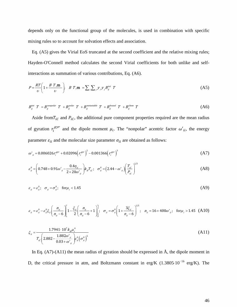
depends only on the functional group of the molecules, is used in combination with specific

mixing rules so to account for solvation effects and association.

Eq. (A5) gives the Virial EoS truncated at the second coefficient and the relative mixing rules;

Hayden-O'Connell method calculates the second Virial coefficients for both unlike and self-

interactions as summation of various contributions, Eq. (A6).

( , )1 ; ( , ) ( )toti j iji j

RT B TP B T y y B Tυ υ

= + =

∑ ∑m m (A5)

( ) ( ) ( ) ( ) ( ) ( )tot nonpolar polar metastable bound chemij ij ij ij ij ijB T B T B T B T B T B T= + + + + (A6)

Aside from𝑇𝑇𝑖𝑖𝑔𝑔 and 𝑑𝑑𝑖𝑖𝑔𝑔, the additional pure component properties required are the mean radius

of gyration 𝑟𝑟𝑖𝑖𝑔𝑔𝑦𝑦𝑐𝑐 and the dipole moment 𝜇𝜇𝑖𝑖. The “nonpolar” acentric factor 𝜔𝜔′𝑖𝑖𝑖𝑖, the energy

parameter 𝜀𝜀𝑖𝑖𝑖𝑖 and the molecular size parameter 𝜎𝜎𝑖𝑖𝑖𝑖 are obtained as follows:

( ) ( )2 3' 0.006026 0.02096 0.001366gyr gyr gyrii i i ir r rω = + − (A7)

( )1/3

0 00.40.748 0.91 ' ; 2.44 '

2 20 'iCii

ii ii B iC ii iiii iC

Tk T

Pη

ε ω σ ωω

= + − = − +

(A8)

0 0; ; for 1.45ii ii ii ii iε ε σ σ µ= = < (A9)

1/3

0 0 0 31 1 ; 1 ; 16 400 ' ; for 1.45

6 2 6 6ii ii ii ii

ii ii ii ii ii ii ii ii iii ii ii

n nn

n n nξ ξ

ε ε ε ξ σ σ ω µ

= − − + = + = + > − − − (A10)

( )

7 4

60 0

1.7941 101.882 '

2.8820.03 '

B iii

iiiC ii ii

ii

k

T

µξ

ωε σ

ω

⋅=

− +

(A11)

In Eq. (A7)-(A11) the mean radius of gyration should be expressed in Å, the dipole moment in

D, the critical pressure in atm, and Boltzmann constant in erg/K (1.3805⋅10−16 erg/K). The

46

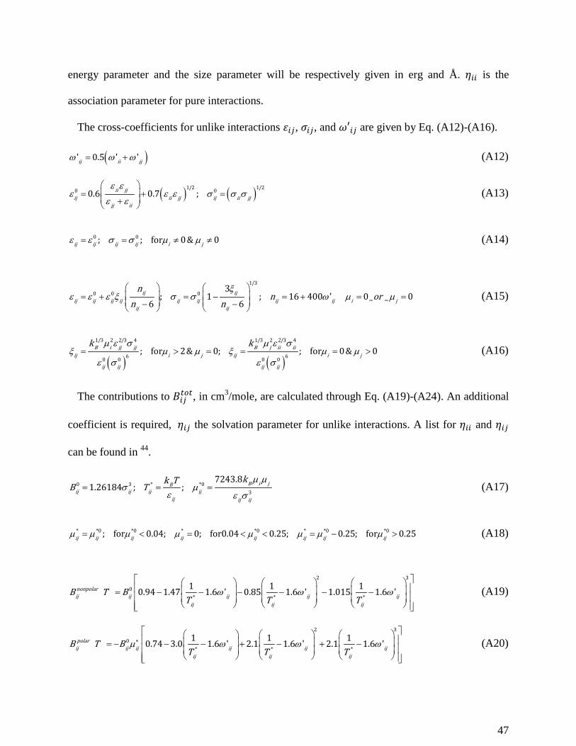
energy parameter and the size parameter will be respectively given in erg and Å. 𝜂𝜂𝑖𝑖𝑖𝑖 is the

association parameter for pure interactions.

The cross-coefficients for unlike interactions 𝜀𝜀𝑖𝑖𝑖𝑖, 𝜎𝜎𝑖𝑖𝑖𝑖, and 𝜔𝜔′𝑖𝑖𝑖𝑖 are given by Eq. (A12)-(A16).

( )' 0.5 ' 'ij ii jjω ω ω= + (A12)

( ) ( )1/2 1/20 00.6 0.7 ;ii jjij ii jj ij ii jj

jj ii

ε εε ε ε σ σ σ

ε ε

= + =

+ (A13)

0 0; ; for 0& 0ij ij ij ij i jε ε σ σ µ µ= = ≠ ≠ (A14)

1/3

0 0 03

; 1 ; 16 400 ' 0_ _ 06 6

ij ijij ij ij ij ij ij ij ij i j

ij ij

nn or

n nξ

ε ε ε ξ σ σ ω µ µ

= + = − = + = = − −

(A15)

( ) ( )

1/3 2 2/3 4 1/3 2 2/3 4

6 60 0 0 0; for 2& 0; ; for 0& 0B i jj jj B j ii ii

ij i j ij i j

ij ij ij ij

k kµ ε σ µ ε σξ µ µ ξ µ µ

ε σ ε σ= > = = = > (A16)

The contributions to 𝐵𝐵𝑖𝑖𝑖𝑖𝑠𝑠𝑠𝑠𝑠𝑠, in cm3/mole, are calculated through Eq. (A19)-(A24). An additional

coefficient is required, 𝜂𝜂𝑖𝑖𝑖𝑖 the solvation parameter for unlike interactions. A list for 𝜂𝜂𝑖𝑖𝑖𝑖 and 𝜂𝜂𝑖𝑖𝑖𝑖

can be found in 44.

0 3 * *03

7243.81.26184 ; ; B i jB

ij ij ij ijij ij ij

kk TB T

µ µσ µ

ε ε σ= = = (A17)

* *0 *0 * *0 * *0 *0; for 0.04; 0; for0.04 0.25; 0.25; for 0.25ij ij ij ij ij ij ij ijµ µ µ µ µ µ µ µ= < = < < = − > (A18)

2 3

0* * *

1 1 1( ) 0.94 1.47 1.6 ' 0.85 1.6 ' 1.015 1.6 'nonpolarij ij ij ij ij

ij ij ij

B T BT T T

ω ω ω = − − − − − −

(A19)

2 3

0* * *

1 1 1( ) 0.74 3.0 1.6 ' 2.1 1.6 ' 2.1 1.6 'polarij ij ij ij ij ij

ij ij ij

B T BT T T

µ ω ω ω∗ = − − − + − + −

(A20)

47

( ) ( )2

0*

1.99 0.2( ) ( ) 0.3 0.05 exp ; for 4.5ijmetastable bound

ij ij ij ij ijij

B T B T BT

µµ η

∗

∗

+ + = − + <

(A21)

( ) ( )0

*

1500 650( ) 1 exp exp 4.27 ; for 4.5

/ / 300ij ijchem

ij ij ij ijij B ij ij B

B T Bk T k

η ηη η

ε ε

= − − < +

(A22)

When compounds with strong association are present in the mixture, 𝜂𝜂𝑖𝑖𝑖𝑖 ≥ 4.5 and/or 𝜂𝜂𝑖𝑖𝑖𝑖 ≥

4.5, the corresponding interactions are treated according to the chemical theory of dimerization.

( )( , ) ( , ) ( , ) ; for 4.5

2ijmetastable bound chem

ij ij ij ij

K T RTB T P B T P B T PP

η

+ + = − ≥

(A23)

( , ) ( , ) ( , ) ( ) ; for 4.5metastable bound chemii ii ii ii ii

RTB T P B T P B T P K TP

η+ + = − ≥ (A24)

DIPPR-105 and DIPPR-116 correlations for saturated liquid volume

The two correlations of relevance for the estimation of the saturated liquid volumes, developed

by the Design Institute for Physical Properties as part of the DIPPR Project 801 37, are reported

below.

4

31 1

1 2

1

DIPPR / cc mol105

lTl

Li

ll

υ

+ −

−⋅ =− (A25)

10.35 2/3 4/3

1 2 3 4 5

DIPP 1/ cc mo116 l 1R ;Li

C

TTl l l l l

υ ττ τ τ τ

−⋅ = = −+ + +

−+

(A26)

The correlation parameters give the saturated liquid volume in cm3 mol-1 when the temperature

is expressed in K.

48

Brelvi-O’Connell correlation for gaseous solute volume at infinite dilution

The Brelvi-O’Connell correlation 38, below presented, can used to estimate the gaseous solute

volume at infinite dilution. The equations are formulated in terms of reduced properties and

relate the compressibility to the reduced density and the partial molar volume to reduced solvent

density.

0.62' '

ln 1 2.4467 2.12074 ; for2.0 ( ' / ) 2.785'

g LCi CiCi iL

i Cg iRTυ υ υ

υ υβ υ υ

∞ − = − + < <

(A27)

0.62 2' ' '

ln 1 3.02214 1.87085 0.71955 ; for2.785 ( ' / ) 3.2'

g LCi Ci CiCi iL L

i Cg i iRTυ υ υ υ

υ υβ υ υ υ

∞ − = − + < <

(A28)

2 3' ' '

ln 1 0.42704 1 2.0890 1 0.42367 1L

C C CL L LRT

υ υ υυβ υ υ υ

+ = − − + − − −

(A29)

In Eq. (A27)-(A28) 𝛽𝛽𝑖𝑖 is the isothermal compressibility of the solvent, 𝜐𝜐′𝑔𝑔𝑖𝑖 and 𝜐𝜐′𝑔𝑔𝑔𝑔 are the

characteristic volumes for the solvent and for the solute; for nonpolar species the characteristic

volume can be taken equal to the critical volume, but for polar species this property tends to be

smaller.

Eq. (A29) is written for a generic component, it can be fitted to liquid compressibility data to

obtain the respective characteristic volume 𝜐𝜐′𝑔𝑔. When used to calculate �̅�𝜐𝑔𝑔∞, it provides the

solvent isothermal compressibility, 𝛽𝛽𝑖𝑖, required in Eq. (A27)-(A28).

Brelvi-O’Connell isothermal equation of state for liquid densities

The equation reported below is the integral form of Eq. (A29) as derived in Brelvi and

O’Connell 59, and it can be used to obtain 𝜐𝜐′𝑔𝑔 from density data only. 𝜌𝜌𝑔𝑔∗ is a scaled density,

where the scaling factor is the characteristic volume of the substance. Once the integral of the

49

reduced isothermal equation is tabulated, the required values at 𝜌𝜌𝑔𝑔∗ |𝑃𝑃1 and 𝜌𝜌𝑔𝑔∗ |𝑃𝑃2 can be obtained

by interpolation.

( ) ( ) ( ) ( )2

1

2 32 1' 'exp 0.42704 1 2.0890 1 0.42367 1 1 ;

R P

R P

C CR R R R R L

P Pd

RT

ρ

ρ

υ υρ ρ ρ ρ ρ

υ

∗

∗

∗ ∗ ∗ ∗ ∗− = − − + − − − − = ∫ (A30)

50

Notation

𝑎𝑎 Peng-Robinson energy parameter defined in Eq. (A2) 𝐴𝐴 two-suffix Margules parameter [J mol-1], Eq. (6), Eq. (17) 𝐴𝐴𝑖𝑖𝑖𝑖 𝐴𝐴𝑖𝑖𝑖𝑖 three-suffix Margules parameters [J mol-1] 𝑏𝑏 Peng-Robinson covolume parameter defined in Eq. (A2) 𝐵𝐵 Second Virial coefficient [m3 mol-1, cm3 mol-1], Eq. (A5) 𝐵𝐵𝑖𝑖𝑖𝑖 Hayden-O'Connell Virial coefficient for self-interactions [cm3 mol-1] defined in Eq. (A6), Eq. (A17)-(A22), Eq. (A24) 𝐵𝐵𝑖𝑖𝑖𝑖 = 𝐵𝐵𝑖𝑖𝑖𝑖 Hayden-O'Connell Virial coefficient for unlike interactions [cm3 mol-1] defined in Eq. (A6), Eq. (A17)-(A22), Eq. (A23) 𝑓𝑓 component fugacity [bar] 𝐺𝐺 Gibbs free energy [J] ℎ1,ℎ2, ℎ3,ℎ4, ℎ5 parameters for the temperature dependent Henry’s law constant, Eq. (8) 𝐻𝐻 Henry’s law constant [bar] 𝑘𝑘𝐵𝐵 Boltzmann constant [1.3805⋅10−16 erg/K] 𝑘𝑘𝑖𝑖𝑖𝑖 = 𝑘𝑘𝑖𝑖𝑖𝑖 𝑘𝑘𝑖𝑖𝑖𝑖 = 0 Peng-Robinson binary interaction parameter, Eq. (A4) 𝐾𝐾𝑖𝑖𝑖𝑖 equilibrium constants for dimerization reaction for pure component, Eq. (A24) 𝐾𝐾𝑖𝑖𝑖𝑖 = 𝐾𝐾𝑖𝑖𝑖𝑖 equilibrium constants for cross-dimerization reaction, Eq. (A23) 𝑙𝑙1, 𝑙𝑙2, 𝑙𝑙3, 𝑙𝑙4, 𝑙𝑙5 parameters for the temperature dependent saturated liquid volume, Eq. (A25) or Eq. (A26) 𝐦𝐦 vapor phase composition tuple [mol] 𝑓𝑓 number of moles of a component [mol] 𝑓𝑓𝑖𝑖𝑖𝑖 Hayden-O'Connell Virial EoS, parameter for n-6 potential model for self-interactions defined in Eq. (A10) 𝑓𝑓𝑖𝑖𝑖𝑖 = 𝑓𝑓𝑖𝑖𝑖𝑖 Hayden-O'Connell Virial EoS, parameter for n-6 potential model for unlike interactions defined in Eq. (A15) 𝐧𝐧 liquid phase composition tuple [mol] 𝐧𝐧𝑘𝑘 𝑘𝑘 ≠ 𝑔𝑔 liquid phase composition tuple except the supercritical component 𝑔𝑔 [mol] 𝑒𝑒1, 𝑒𝑒2,𝑒𝑒3 ,𝑒𝑒4, 𝑒𝑒5, 𝑒𝑒6 parameters for the extended Antoine equation, Eq. (7) 𝑑𝑑 pressure [bar] 𝑞𝑞 component surface parameter for UNIQUAC equation, Eq. (22)-(23) 𝑟𝑟 component size parameter for UNIQUAC equation, Eq. (22) 𝑟𝑟𝑔𝑔𝑖𝑖𝑐𝑐 mean radius of gyration for the Hayden-O'Connell Virial EoS [Å], Eq. (A7) 𝑅𝑅 gas constant [8.314472 J K-1 mol-1, 83.14460 cm3 bar K−1 mol−1, 1.98635 cal K−1 mol−1] 𝑆𝑆 entropy [J K-1] 𝑇𝑇 temperature [K] 𝑇𝑇𝑖𝑖𝑖𝑖∗ Hayden-O'Connell Virial EoS, scaled temperature for self-interactions defined in Eq. (A17) 𝑇𝑇𝑖𝑖𝑖𝑖∗ = 𝑇𝑇𝑖𝑖𝑖𝑖∗ Hayden-O'Connell Virial EoS, scaled temperature for unlike interactions defined in Eq. (A17) 𝑓𝑓𝑖𝑖𝑖𝑖 UNIQUAC self-interaction parameter [J mol-1] defined in Eq. (25) or Eq. (26) 𝑓𝑓𝑖𝑖𝑖𝑖 = 𝑓𝑓𝑖𝑖𝑖𝑖 UNIQUAC unlike interaction parameter [J mol-1] defined in Eq. (25) or Eq. (26) 𝑓𝑓𝑇𝑇0,𝑓𝑓𝑇𝑇1, 𝑓𝑓𝑇𝑇2, 𝑓𝑓𝑇𝑇3 parameters for the temperature dependent UNIQUAC interaction energies, Eq. (25), Eq. (A1) 𝑓𝑓′𝑠𝑠 , 𝑓𝑓′𝑏𝑏 ,𝑓𝑓′𝑐𝑐 ,𝑓𝑓′𝑑𝑑 parameters for the temperature dependent UNIQUAC interaction energies, Eq. (26), Eq. (A1) 𝛥𝛥𝑓𝑓𝑖𝑖𝑖𝑖 ≠ 𝛥𝛥𝑓𝑓𝑖𝑖𝑖𝑖 UNIQUAC delta interaction coefficients [J mol-1] defined in Eq. (24) 𝑉𝑉 volume [m3] 𝑥𝑥 component mole fraction in the liquid phase/in a generic phase 𝑦𝑦 component mole fraction in the vapor phase 𝑧𝑧 number of molecules coordinated to a central one for UNIQUAC equation, Eq. (22)

𝛼𝛼 coefficient for gas solubility in mixed solvents defined in Eq. (17)/coefficient for Peng-Robinson defined in Eq. (A3) 𝛽𝛽 isothermal compressibility [Pa-1], Eq. (A27)-(A29) 𝛾𝛾 component symmetric activity coefficient 𝛾𝛾∗ component un-symmetric activity coefficient 𝛿𝛿 component solubility parameter for Hildebrand equation [cal0.5 cc0.5], Eq. (15) 𝜀𝜀𝑖𝑖𝑖𝑖 Hayden-O'Connell Virial EoS, energy parameter for self-interactions [erg] defined in Eq. (A9)-(A10) 𝜀𝜀𝑖𝑖𝑖𝑖 = 𝜀𝜀𝑖𝑖𝑖𝑖 Hayden-O'Connell Virial EoS, energy parameter for unlike interactions [erg] defined in Eq. (A14)-(A15) 𝜂𝜂𝑖𝑖𝑖𝑖 Hayden-O'Connell Virial EoS, association parameter for pure interactions, Eq. (A8), Eq. (A22) 𝜂𝜂𝑖𝑖𝑖𝑖 = 𝜂𝜂𝑖𝑖𝑖𝑖 Hayden-O'Connell Virial EoS, solvation parameter for unlike interactions, Eq. (A8), Eq. (A22) 𝜃𝜃 component surface fraction for UNIQUAC equation defined in Eq. (22) 𝜇𝜇 Hayden-O'Connell Virial EoS, dipole moment [D], Eq. (A11), Eq. (A16), Eq. (17) 𝜇𝜇𝑖𝑖𝑖𝑖∗ Hayden-O'Connell Virial EoS, reduced dipole moment for self-interactions defined in Eq. (A18) 𝜇𝜇𝑖𝑖𝑖𝑖∗ = 𝜇𝜇𝑖𝑖𝑖𝑖∗ Hayden-O'Connell Virial EoS, reduced dipole moment for unlike interactions defined in Eq. (A18) 𝜉𝜉𝑖𝑖𝑖𝑖 Hayden-O'Connell Virial EoS, angle averaged polar effect for self-interactions defined in Eq. (A11) 𝜉𝜉𝑖𝑖𝑖𝑖 = 𝜉𝜉𝑖𝑖𝑖𝑖 Hayden-O'Connell Virial EoS, angle averaged polar effect for unlike interactions defined in Eq. (A16) 𝜌𝜌𝑔𝑔∗ scaled density respect to the characteristic molar volume for Brelvi-O’Connell correlation defined in Eq. (A1) 𝜎𝜎𝑖𝑖𝑖𝑖 Hayden-O'Connell Virial EoS, size parameter for self-interactions [Å] defined in Eq. (A9)-(A10) 𝜎𝜎𝑖𝑖𝑖𝑖 = 𝜎𝜎𝑖𝑖𝑖𝑖 Hayden-O'Connell Virial EoS, size parameter for unlike interactions [Å] defined in Eq. (A14)-(A15) 𝜏𝜏 DIPPR-116 coefficient defined in Eq. (A26) 𝜏𝜏𝑖𝑖𝑖𝑖 ≠ 𝜏𝜏𝑖𝑖𝑖𝑖 coefficients for UNIQUAC equation defined in Eq. (23) 𝜐𝜐 component molar volume [m3 mol-1, cm3 mol-1] 𝜐𝜐′𝑔𝑔 characteristic molar volume for Brelvi-O’Connell correlation [cm3 mol-1], Eq. (A27)-(A29), Eq. (A1) 𝜑𝜑 component fugacity coefficient 𝛷𝛷 component volume fraction for UNIQUAC equation defined in Eq. (22) 𝜔𝜔 acentric factor for Peng-Robinson EoS, Eq. (A3) 𝜔𝜔′𝑖𝑖𝑖𝑖 Hayden-O'Connell Virial EoS, “nonpolar” acentric factor for self-interactions defined in Eq. (A7) 𝜔𝜔′𝑖𝑖𝑖𝑖 = 𝜔𝜔′𝑖𝑖𝑖𝑖 Hayden-O'Connell Virial EoS, “nonpolar” acentric factor for unlike interactions Eq. (A12)

51

Subscripts

Superscripts

Accents

𝐶𝐶 critic property 𝑔𝑔 supercritical component 𝑖𝑖 generic component/pure solvent/solvent forming a mixture 𝑗𝑗 generic component/pure solvent/solvent forming a mixture 𝑘𝑘 generic component/data point index 𝑅𝑅 reduced property 𝑠𝑠𝑠𝑠𝑙𝑙 single solvent system or mixed solvent system z binary system index 0 reference temperature

𝑏𝑏𝑠𝑠𝑓𝑓𝑓𝑓𝑑𝑑 contribution to Hayden-O'Connell Virial coefficient due to physically bound molecule pair 𝑐𝑐𝑎𝑎𝑙𝑙𝑐𝑐 calculated value 𝑐𝑐ℎ𝑒𝑒𝑚𝑚 contribution to Hayden-O'Connell Virial coefficient due to chemically bound molecule pair 𝑐𝑐𝑠𝑠𝑟𝑟𝑟𝑟 value from Prausnitz and Shair correlation 𝐶𝐶 UNIQUAC combinatorial contribution to the activity coefficient 𝑒𝑒𝑥𝑥𝑒𝑒 experimental value 𝐸𝐸 excess property ℎ𝑦𝑦𝑒𝑒 hypothetical liquid standard state 𝑓𝑓𝑠𝑠𝑓𝑓𝑒𝑒𝑠𝑠𝑙𝑙𝑎𝑎𝑟𝑟 contribution to Hayden-O'Connell Virial coefficient due to non-polar forces for pair interaction 𝑒𝑒𝑠𝑠𝑙𝑙𝑎𝑎𝑟𝑟 contribution to Hayden-O'Connell Virial coefficient due to polar forces for pair interaction 𝑅𝑅 UNIQUAC residual contribution to the activity coefficient 𝑠𝑠𝑎𝑎𝑠𝑠 pure solvent saturation condition/mixed solvents saturation condition 𝑠𝑠𝑠𝑠𝑠𝑠 net contribution to Hayden-O'Connell Virial coefficient for pair interaction 𝑉𝑉 vapor phase 0 Hayden-O'Connell Virial EoS transitory variable ∞ infinitely dilute liquid solution condition

^ mixture property ¯ partial property

52

AUTHOR INFORMATION

Corresponding Author

*Philip L. Fosbøl, E-mail: plf@kt.dtu.dk

ACKNOWLEDGMENT

The authors acknowledge the financial support from the Technical University of Denmark and

Innovation Fund Denmark in connection with the SYNFERON project.

REFERENCES

(1) Higman, C. GSTC Syngas Database: 2017 Update http://worldctx.com/wp-

content/uploads/HigmanGSTC2017.pdf (accessed Feb 13, 2018).

(2) Daniell, J.; Köpke, M.; Simpson, S. D. Commercial Biomass Syngas Fermentation.

Energies 2012, 5 (12), 5372–5417.

(3) Bredwell, M. D.; Srivastava, P.; Worden, R. M. Reactor Design Issues for Synthesis-Gas

Fermentations. Biotechnol. Prog. 1999, 15 (5), 834–844.

(4) Prausnitz, J. M.; Lichtenthaler, R. N.; de Azevedo, E. G. Molecular Thermodynamics of

Fluid-Phase Equilibria, third.; Prentice Hall: New Jersey, 1998.

(5) Carroll, J. J.; Mather, A. E. The System Carbon Dioxide-Water and the Krichevsky-

Kasarnovsky Equation. J. Solution Chem. 1992, 21 (7), 607–621.

(6) Margules, M. Über Die Zusammensetzung Der Gesättigten Dämpfe von Mischungen.

Sitzungsberichte der Kais. Akadamie der Wissenschaften Wien Math. Klasse II 1895, 104,

1243–1278.

53

(7) Duan, Z.; Sun, R. An Improved Model Calculating CO2 Solubility in Pure Water and

Aqueous NaCl Solutions from 273 to 533 K and from 0 to 2000 Bar. Chem. Geol. 2003,

193 (3–4), 257–271.

(8) Pitzer, K. S. Thermodynamics of Electrolytes. I. Theoretical Basis and General Equations.

J. Phys. Chem. 1973, 77, 268–277.

(9) Huron, M.-J.; Vidal, J. New Mixing Rules in Simple Equations of State for. Fluid Phase

Equilib. 1979, 3 (4), 255–271.

(10) Pedersen, K. S.; Milter, J.; Rasmussen, C. P. Mutual Solubility of Water and a Reservoir

Fluid at High Temperatures and Pressures. Fluid Phase Equilib. 2001, 189, 85–97.

(11) Kontogeorgis, G. M.; Voutsas, E. C.; Yakoumis, I. V.; Tassios, D. P. An Equation of State

for Associating Fluids. Ind. Eng. Chem. Res. 1996, 35 (11), 4310–4318.

(12) Chapman, W. G.; Gubbins, K. E.; Jackson, G.; Radosz, M. SAFT: Equation-of-State

Solution Model for Associating Fluids. Fluid Phase Equilib. 1989, 52, 31–38.

(13) Kontogeorgis, G. M.; Michelsen, M. L.; Folas, G. K.; Derawi, S.; Von Solms, N.; Stenby,

E. H. Ten Years with the CPA (Cubic-Plus-Association) Equation of State. Part 2. Cross-

Associating and Multicomponent Systems. Ind. Eng. Chem. Res. 2006, 45, 4869–4878.

(14) Austegard, A.; Solbraa, E.; de Koeijer, G.; Mølnvik, M. J. Thermodynamic Models for

Calculating Mutual Solubilities in H2O-CO2-CH4 Mixtures. Chem. Eng. Res. Des. 2006,

84 (9 A), 781–794.

(15) Perakis, C.; Voutsas, E.; Magoulas, K.; Tassios, D. Thermodynamic Modeling of the

Vapor-Liquid Equilibrium of the water/ethanol/CO2 System. Fluid Phase Equilib. 2006,

54

243 (1–2), 142–150.

(16) García, A. V.; Thomsen, K.; Stenby, E. H. Prediction of Mineral Scale Formation in

Geothermal and Oilfield Operations Using the Extended UNIQUAC Model. Part II.

Carbonate-Scaling Minerals. Geothermics 2006, 35 (3), 239–284.

(17) Spycher, N.; Pruess, K. A Phase-Partitioning Model for CO2-Brine Mixtures at Elevated

Temperatures and Pressures: Application to CO2-Enhanced Geothermal Systems. Transp.

Porous Media 2010, 82 (1), 173–196.

(18) Hou, S.-X.; Maitland, G. C.; Trusler, J. P. M. Measurement and Modeling of the Phase

Behavior of the (Carbon Dioxide+water) Mixture at Temperatures from 298.15K to

448.15K. J. Supercrit. Fluids 2013, 73, 87–96.

(19) Mao, S.; Zhang, D.; Li, Y.; Liu, N. An Improved Model for Calculating CO2 Solubility in

Aqueous NaCl Solutions and the Application to CO2-H2O-NaCl Fluid Inclusions. Chem.

Geol. 2013, 347, 43–58.

(20) Venkatraman, A.; Lake, L. W.; Johns, R. T. Gibbs Free Energy Minimization for

Prediction of Solubility of Acid Gases in Water. Ind. Eng. Chem. Res. 2014, 53 (14),

6157–6168.

(21) F. Najmuldeen, G.; Jasim Hadi, G.; Jasim Hadi, A.; Ahmed, I. Gas-Liquid Equilibrium

Prediction of Ternary System (CO2-Ethanol-Water) at Moderate Pressures and Different

Temperatures Using SRK-EOS. Phys. Chem. 2012, 2 (1), 1–5.

(22) Nakayama, T.; Sagara, H.; Arai, K.; Saito, S. An Equation for the Excess Gibbs Energy of

Expandable Liquid Mixtures. J. Chem. Eng. Japan 1988, 21, 509–515.

55

(23) Michelsen, M. L.; Mollerup, J. M. Thermodynamic Models: Fundamentals &

Computational Aspects, second.; Tie-Line: Holte, 2007.

(24) Sander, B. Extended UNIFAC/UNIQUAC Models for 1) Gas Solubility Calculations and

2) Electrolyte Solutions, Danmarks Tekniske Højskole, 1984.

(25) Krichevsky, I. R.; Kasarnovsky, J. S. Thermodynamical Calculations of Solubilities of

Nitrogen and Hydrogen in Water at High Pressures. J. Am. Chem. Soc. 1935, 57 (11),

2168–2171.

(26) Aspen Technology, Inc, AspenTech http://www.aspentech.com.

(27) Glew, D. N. Aqueous Solubility and the Gas-Hydrates. The Methane-Water System. J.

Phys. Chem. 1962, 66, 605–609.

(28) Nocon, G.; Weidlich, U.; Gmehling, J.; Onken, U. Prediction of Gas Solubilities by a

Modified UNIFAC Equation. Berichte der Bunsengesellschaft für Phys. Chemie 1983, 87,

17–23.

(29) Purwanto; Deshpande, R. M.; Chaudhari, R. V.; Delmas, H. Solubility of Hydrogen,

Carbon Monoxide, and 1-Octene in Various Solvents and Solvent Mixtures. J. Chem. Eng.

Data 1996, 41, 1414–1417.

(30) Prausnitz, J. M.; Shair, F. H. Thermodynamic Correlation of Gas Solubilities. AIChE J.

1961, 7 (4), 682–687.

(31) McKetta Jr., J. J.; Yen, L. C. A Thermodynamic Correlation of Nonpolar Gas Solubilities

in Polar, Nonassociated Liquids. AIChE J. 1962, 8 (4), 501–507.

56

(32) O’Connell, J. P.; Prausnitz, J. M. Thermodynamics of Gas Solubility in Mixed Solvents.

Ind. Eng. Chem. Fundam. 1964, 3 (4), 347–351.

(33) Abrams, D. S.; Prausnitz, J. M. Statistical Thermodynamics of Liquid Mixtures: A New

Expression for the Excess Gibbs Energy of Partly or Completely Miscible Systems.

AIChE J. 1975, 21 (1), 116–128.

(34) Bondi, A. Van Der Waals Volumes and Radii. J. Phys. Chem. 1964, 68 (3), 441–451.

(35) Peng, D. Y.; Robinson, D. B. A New Two-Constant Equation of State. Ind. Eng. Chem.

Fundam. 1976, 15 (1), 59–64.

(36) Hayden, J. G.; O’Connell, J. P. A Generalized Method for Predicting Second Virial

Coefficients. Ind. Eng. Chem. Process Des. Dev. 1975, 14 (3), 209–216.

(37) Brigham Young University (BYU), DIADEM Professional DIPPR Information and Data

Evaluation Manager http://dechema.de/en/dippr801.html.

(38) Brelvi, S. W.; O’Connell, J. P. Correspondling States Correlations for Liquid

Compressibility and Partial Molal Volumes of Gases at Infinite Dilution in Liquids.

AIChE J. 1972, 18 (6), 1239–1243.

(39) Chemistry Data Series http://dechema.de/en/CDS.html.

(40) Thomsen, K.; Rasmussen, P.; Gani, R. Correlation and Prediction of Thermal Properties

and Phase Behaviour for a Class of Aqueous Electrolyte Systems. Chem. Eng. Sci. 1996,

51, 3675–3683.

(41) Jónasson, A.; Persson, O.; Rasmussen, P.; Soave, S. G. Vapor-Liquid Equilibria of

57

Systems Containing Acetic Acid and Gaseous Components. Measurements and

Calculations by a Cubic Equation of State. Fluid Phase Equilib. 1998, 152, 67–94.

(42) Maxted, E. B.; Moon, C. H. The Temperature Coefficient of the Solubility of Hydrogen in

Organic Solvents. Trans. Faraday Soc. 1936, 32, 769–775.

(43) Just, G. Löslichkeit von Gasen in Organischen Lösungsmitteln. Zeitschrift für Phys.

Chemie 1901, 37, 342–367.

(44) Prausnitz, J. M.; Anderson, T.; Grens, E.; Eckert, C.; Hsieh, R.; O’Connell, J. P. Computer

Calculations for Multicomponent Vapor-Liquid and Liquid-Liquid Equilibria, first.;

Prentice Hall: Englewood Cliffs, New Jersey, 1980.

(45) Batsanov, S. S. Van Der Waals Radii of Hydrogen in Gas-Phase and Condensed

Molecules. Struct. Chem. 1999, 10 (6), 395–400.

(46) Sun, T. F.; Ten Seldam, C. A.; Kortbeek, P. J.; Trappeniers, N. J.; Biswas, S. N. Acoustic

and Thermodynamic Properties of Ethanol from 273.15 to 333.15 K and up to 280 MPa.

Phys. Chem. Liq. 1988, 18, 107–116.

(47) Takiguchi, Y.; Uematsu, M. Densities for Liquid Ethanol in the Temperature Range from

310 K to 480 K at Pressures up to 200 MPa. J. Chem. Thermodyn. 1996, 28, 7–16.

(48) Vong, W. T.; Tsai, F. N. Densities, Molar Volumes, Thermal Expansion Coefficients, and

Isothermal Compressibilities of Organic Acids from 293.15 K to 323.15 K and at

Pressures up to 25 MPa. J. Chem. Eng. Data 1997, 42, 1116–1120.

(49) Rackett, H. G. Equation of State for Saturated Liquids. J. Chem. Eng. Data 1970, 15, 514–

517.

58

(50) Valtz, A.; Chapoy, A.; Coquelet, C.; Paricaud, P.; Richon, D. Vapour-Liquid Equilibria in

the Carbon Dioxide-Water System, Measurement and Modelling from 278.2 to 318.2 K.

Fluid Phase Equilib. 2004, 226, 333–344.

(51) King, M. B.; Mubarak, A.; Kim, J. D.; Bott, T. R. The Mutual Solubilities of Water with

Supercritical and Liquid Carbon Dioxide. J. Supercrit. Fluids 1992, 5, 296–302.

(52) Nakayama, T.; Sagara, H. High Pressure Liquid-Liquid Equilibria for the System of

Water, Ethanol and 1,1-Difluoroethane at 323.2 K. Fluid Phase Equilib. 1987, 38, 109–

127.

(53) Wiebe, R.; Gaddy, V. L. The Solubility of Carbon Dioxide in Water at Various

Temperatures from 12 to 40° and at Pressures to 500 Atmospheres. Critical Phenomena. J.

Am. Chem. Soc. 1940, 62 (4), 815–817.

(54) Kiepe, J.; Horstmann, S.; Fischer, K.; Gmehling, J. Experimental Determination and

Prediction of Gas Solubility Data for CO2 + H2O Mixtures Containing NaCl or KCl at

Temperatures between 313 and 393 K and Pressures up to 10 MPa. Ind. Eng. Chem. Res.

2002, 41 (17), 4393–4398.

(55) Jung, J.; Knacke, O.; Neuschütz, D. Löslichkeit von Kohlenmonoxid Und Wasserstoff in

Wasser Bis 300°C. Chemie Ing. Tech. 1971, 43, 112–116.

(56) Song, K. Y.; Feneyrou, G.; Fleyfel, F.; Martin, R.; Lievois, J.; Kobayashi, R. Solubility

Measurements of Methane and Ethane in Water at and near Hydrate Conditions. Fluid

Phase Equilib. 1997, 128, 249–259.

(57) Brunner, E.; Hültenschmidt, W. Fluid Mixtures at High Pressures VIII. Isothermal Phase

59

Equilibria in the Binary Mixtures Consisting of (Ethanol+hydrogen or Methane or

Ethane). J. Chem. Thermodyn. 1990, 22, 73–84.

(58) Frolich, K.; Tauch, E. J.; Hogan, J. J.; Peer, A. A. Solubilities of Gases in Liquids at High

Pressure. Ind. Eng. Chem. 1931, 23, 548–550.

(59) Brelvi, S. W.; O’Connell, J. P. A Generalized Isothermal Equation of State for Dense

Liquids. AIChE J. 1975, 21, 171–173.

60

61