Solitary waves and N -particle algorithms for a class of Euler-Poincareequations

By Roberto Camassa, Dongyang Kuang and Long Lee

We study a class of partial differential equations (PDEs) in the family of the so-called Euler-Poincare differential systems, with the aim of developing a foundation for numerical algorithmsof their solutions. This requires particular attention to the mathematical properties of this sys-tem when the associated class of elliptic operators possesses non-smooth kernels. By castingthe system in its Lagrangian (or characteristics) form, we first formulate a particles systemalgorithm in free space with homogeneous Dirichlet boundary conditions for the evolving fields.We next examine the deformation of the system when non-homogeneous “constant stream”boundary conditions are assumed. We show how this simple change at the boundary deeplyaffects the nature of the evolution, from hyperbolic-like to dispersive with a non-trivial dis-persion relation, and examine the potentially regularizing properties of singular kernels offeredby this deformation. From the particle algorithm viewpoint, kernel singularities affect theexistence and uniqueness of solutions to the corresponding ordinary differential equations sys-tems. We illustrate this with the case when the operator kernel assumes a conical shape overthe spatial variables, and examine in detail two-particle dynamics under the resulting lack ofLipschitz-continuity. Curiously, we find that for the conically-shaped kernels the motion ofthe related two-dimensional waves can become completely integrable under appropriate initialdata. This reduction projects the two-dimensional system to the one-dimensional completelyintegrable Shallow-Water equation [Camassa, R. and Holm, D. D., Phys. Rev. Lett., 71,1961-1964, 1993], while retaining the full dependence on two spatial dimensions for the singlechannel solutions. Finally, by comparing with an operator-splitting pseudospectral method weillustrate the performance of the particle algorithms with respect to their Eulerian counterpartfor this class of non-smooth kernels.

keywords Euler-Poincare differential equations, diffeomorphisms, Lagrangian formulation, dispersive, particle algo-

rithms, completely integrable, Shallow-Water equation

1. Introduction

The Euler-Poincare differential equations, also called the Euler equations for planar diffeo-morphisms, originate in models of template matching and are of general interest as evolutionequations on Riemannian manifolds endowed with Sobolev metrics [1–5]. In one spatial di-mension, the system of the partial differential equations (PDEs) we consider in this paper mayreduce to a completely integrable equation arising as a model of long wave evolution in shallow

Address for correspondence: Dongyang Kuang, Department of Mathematics, University of Wyoming, Laramie, WY82071;email: dykuang@outlook.com

DOI: 10.1111/SAP.M20140252 1STUDIES IN APPLIED MATHEMATICS 00:1–32c© Wiley Periodicals, Inc., A Wiley Company

2

water, derived in [6, 7] (hereafter referred to as the SW – for Shallow-Water – equation). Inthis physical context, these PDEs can be used as a model of the competition between nonlinearand dispersive effects, whose intertwined properties contribute to the rich dynamics exhibitedby this class of nonlinear evolution equations.

One notable feature of the model PDEs under study (also known as the “EPDiff” differen-tial equations in some literature) is that they admit traveling-wave weak-solutions, for whichthe momentum-like variable may be viewed as concentrated at a single point as if it were a“particle.” In fact, these particles are reminiscent of point vortices in Euler equations, whichare widely studied in the literature both for their inherent interest as dynamical systems andas a foundation for numerical algorithms for the evolution of general Euler solutions. Similarlyto this latter case, once projected onto the particle solution class the evolution of the PDEs canbe written in the form of a finite-dimensional particle system of ordinary different equations(ODEs). We will refer to this system of ODEs as the N -particle finite-dimensional dynamicalsystem, or N -particle system.

For nonlinear dispersive equations, the interplay between nonlinearity and dispersion is oftenunderstood as the mechanism underlying the existence of traveling wave solutions. However,the way in which solitary waves emerge and can become the dominant structure in the long timeevolution out of generic initial conditions can take various forms, depending on the structureof the equations, especially in multiple space dimensions. Study of the N -particle system fora class of the model PDEs, where the interplay between dispersion and nonlinearity is variedcontinuously within a one-parameter family, is a convenient way to shed light on this as wellas to investigate the role played by traveling waves in the long time evolution from a range ofinitial data.

An interesting application for the N -particle system is template matching. This is com-monly used in problems of image reconstruction and pattern recognition [8, 9]. Templatematching can be formulated as an variational problem, such as finding the shortest or leastexpensive path of continuous deformation of one geometric object (reference template) into an-other one (target template). In this context, the time-dependent deformation process producesgeodesic evolution equations which falls into the Euler-Poincare theory [3]. A practical applica-tion for template matching is computational anatomy (CA) [10], whereby a medical image canbe discretized into a set of so-called landmark points, which in turn can be represented by theN -particle system of the model PDEs. The template matching problem, in terms of landmarkpoints, becomes the landmark-matching problem [3,11]. While the template matching problemis related to the issue of comparing two geometric objects, and thus more concerned with avariational boundary-value problem, the initial-value problem associated to the integration ofthe model equations and/or their N -particle system has important consequences for applica-tions, especially for designing numerical matching procedures [3, 12, 13]. As noted above, theN -particle algorithms and dynamics play an important role in both the model PDEs and theirapplications. However, despite some notable efforts [2, 14], there are aspects of the N -particlesystems and their dynamics that have not been thoroughly investigated, particularly whencertain smoothness properties are not satisfied. The aim of this paper is to examine someof these aspects, with the brooder goal of establishing the foundations of potentially efficientnumerical algorithms for the solution of this class of model PDEs.

The steps we take towards implementing this goal are as follows. We first introduce the La-grangian formulation of for the class of PDEs under investigation, which allows us to discretizethe resulting integral-differential equations to obtain the N -particle systems for the modelPDEs. Our approach introduces a mesh size (e.g., dx dy in two dimensions) naturally andexplicitly, a necessary step for proving the convergence of the particle algorithm. The singularnature of some the particle solutions suggests that a form of regularization might be neededin order to implement numerical algorithms. We examine a possible class of regularizations of

Wave dynamics for Euler-Poincare equations 3

the model PDE, and show that this follows simply from assuming non-zero constant boundaryconditions on the evolving fields. The deformation leads to non-trivial dispersive evolution, andthe corresponding dispersion relation explicitly displays the limitations that this can presentwhen used as regularization for non-smooth solutions (unlike its one-dimensional counterparts,see e.g. [15]). We illustrate two-particle dynamics for non-Lipschitz kernels (with particularattention to the example where the power of the associated elliptic operator is equal to 3/2)via direct numerical simulations and analysis. We analyze the scattering properties under theloss of uniqueness of ODE solutions due to these non-Lipschitz kernels. We also show thatwhen the motion of these particles is confined to a straight line, the dynamics of the associatedsolitary waves (dubbed as “conons”) coincides with that of the SW equation and is thereforecompletely integrable, even though the “single channel” solution retains its dependence on twospatial dimensions. Finally, we demonstrate that the N -particle system can be advantageousfor solving the model PDEs with non-smooth solutions, and is also robust enough to capturemore regular solutions, by comparing with an operator-splitting pseudospectral method forsolving the Eulerian form of the model equation.

2. Equations of motion

By using index notation with Einstein convention on sums over repeated indexes for the (col-umn) vectors m ≡ {mα}nα=1 and u ≡ {uα}nα=1, the system of equations can be written as

∂tmα + uβ∂βmα +mβ∂αuβ +mα∂βuβ = 0 , (1)

or, in short-hand vector notation,

mt + (u · ∇)m+m · (∇u)T +m(∇ · u) = 0, (2)

with t ∈ R+, x,u and m ∈ Rn, and spatial partial derivatives are labeled by coordinate index.For ease of notation, here and throughout the rest of the paper we will use Greek alphabetindexes to label coordinates, to distinguish them from particle labels (see below) in Latinalphabet, and suppress explicit argument dependences in the notation unless this becomesnecessary to avoid confusion. The field u and its associated momentum-like variable m areformally related by an elliptic operator L

m = Lu . (3)

With boundary vanishing boundary conditions at infinity, the operator L is assumed to beinvertible, with its inverse being explicitly written in terms of the corresponding Green functionG, so that u can also be represented by the convolution

u = G ∗m. (4)

In this paper we will restrict our attention to the particular choice of L ≡ Lb as the (Yukawa)operator defined by

Lb = (I − a2∇2)b, (5)

for b > 0. Further, for the domain of Lb we will take the Schwartz space of rapidly decayingfunctions in Rn. For any b > 0, including non-integer values, equation (3) can be defined inFourier space,

u = (Lb)−1m, where (Lb)−1 =1

(1 + a2|k|2)b, |k| =

√k2

1 + k22 · · ·+ k2

n, (6)

where kα is the αth wavenumber. Since Lb is rotationally invariant and diagonal, then G(x) =

Gb−n/2(|x|)I for a scalar function Gb−n/2, with |x| =√x2

1 + x22 + ·+ x2

n. The scalar Green

4

function Gb−n/2 can be obtained by a combination of Bessel and Gamma functions,

Gb−n/2(|x|) =2n/2−b

(2πa)n/2abΓ(b)|x|b−n/2Kb−n/2

( |x|a

), (7)

where Kb−n/2 is the modified Bessel function of the second kind of order b − n/2 and Γ(b) isthe usual notation for the Gamma function [11].

2.1. Lagrangian formulation

Equation (1) is the Eulerian counterpart of a Lagrangian formulation obtained from the char-acteristics x = q(ξ, t)

dq

dt≡ u(q(ξ, t)) , q(ξ, 0) = ξ , (8)

by defining the conjugate field p(ξ, t)

m(q(ξ, t), t

)≡ p(ξ, t)

J(ξ, t), (9)

where J(ξ, t) is the Jacobian determinant of the diffeomorphism x = q(ξ, t) parametrized bytime t,

J(ξ, t) ≡ det

(∂xi∂ξj

),

with J(ξ, 0) = 1. For as long as J(ξ, t) 6= 0 the definition (9) is well posed, and the evolutionequation preserves the smoothness of the initial data. Thus, from the characteristic formulationof equation (1), local well posedness and existence of solutions can be readily established. Thewell known property of determinant differentiation

dJ

dt= J ∇ · u (10)

shows that the m evolution in equation (1), with our choice of symmetric Green functions, isdefined by

dp

dt= −

∫RnG′b−n/2

(|q(ξ, t)− q(η, t)|

) q(ξ, t)− q(η, t)

|q(ξ, t)− q(η, t)| p(ξ, t) · p(η, t) dVη , (11)

where the integration is taken with the measure dVη of Rn. In terms of these characteristicvariables, the system formed by equation (8), rewritten as

dq

dt=

∫RnGb−n/2

(|q(ξ, t)− q(η, t)|

)p(η, t) dVη , (12)

and equation (11) constitutes the Lagrangian formulation of equation (1). In this form, theequations of motion are a canonical Hamiltonian system with respect to variational derivativesδ/δq and δ/δp

q(ξ, t) =δH

δp, p(ξ, t) = −δH

δq, (13)

of the Hamiltonian functional

H ≡ 1

2

∫Rn

∫RnGb−n/2

(|q(ξ, t)− q(η, t)|

)p(ξ, t) · p(η, t) dVξ dVη . (14)

Wave dynamics for Euler-Poincare equations 5

It is straightforward to check that substituting Eq. (14) into Eq. (13) yields Eqs. (12) and(11), which is equivalent to the model PDEs (2). Hence the canonical Hamiltonian systemforms our model equations.

The Lagrangian version of equation (1) shows that along characteristics q(ξ, t) the evolutionof the momentum-like variables p(ξ, t) is tied to that of the Jacobian matrix ∂βqα(ξ, t) by theinitial conditions p(ξ, 0),

pα(ξ, t)∂qα∂ξβ

(ξ, t) = pβ(ξ, 0) (15)

(sum over repeated index), as it can readily be verified by system (11),(12) and the initialcondition for characteristics ∂βqα(ξ, 0) = δαβ. This is the analog of the constraint evolutionfor the one-dimensional SW equation [16], and can be used similarly to monitor the error ofLagrangian numerical schemes to solve system (13). In Appendix A, we provide details on theconnection of the Lagrangian formulation with the Eulerian form of system (2).

2.2. Nonhomogeneous boundary conditions and dispersive deformations

One of the simplest settings removing the assumption of homogeneous boundary conditionsis that of an infinite domain with u(x, ·) → κ as x → ∞ sufficiently fast, for some constantvector κ. This is most conveniently analyzed by defining the shifted field

u ≡ u+ κ , (16)

where u is assumed to decay rapidly at infinity. With the “Galilean boost”

x = x− κt, t = t , (17)

system (2) maintains its form as the contributions from the boost and the u shift cancel out,

mt − κ · ∇m+ ((u+ κ) · ∇)m+m · (∇u)T +m(∇ · u) = 0,

with obvious meaning of the operator ∇. The formalism developed for homogeneous bound-ary conditions in free space can be applied by modifying the link between m and u by thecorresponding shift

m ≡m+ κ (18)

so that domain of the operator L can remain the same (e.g., the Schwartz space for u initialdata), and

m ≡ Luso that

mt + (u · ∇)m+ (m+ κ) · (∇u)T + (m+ κ)(∇ · u) = 0. (19)

Dropping tildes from now on, this deformation of the original evolution equation (2), againwith homogeneous boundary conditions for the new variables, can be cast in terms of charac-teristics as done for system (11),(12), by changing the boundary conditions for the momentumvector p. If we let

p(ξ, t)→ κ ≡ const. as |ξ| → ∞ ,

with

m(q(ξ, t), t

)+ κ ≡ p(ξ, t)

J(ξ, t), (20)

6

and

dq

dt= −κ+

∫RnGb−n/2

(|q(ξ, t)− q(η, t)|

)p(η, t) dVη , (21)

the resulting system is the dispersive counterpart of the evolution equation in Eulerian form

mt + (u · ∇)m+ (m+ κ) · (∇u)T + (m+ κ)(∇ · u) = 0. (22)

The corresponding Hamiltonian is

H ≡ 1

2

∫Rn

∫Rn

[Gb−n/2

(|q(ξ, t)−q(η, t)|

)p(ξ, t) ·p(η, t)−κ · (p(ξ, t) +p(η, t))

]dVξ dVη . (23)

The shifted model (22) reveals that imposing constant boundary conditions at infinity forsystem (2) makes the time evolution of the dependent variables u and m linearly dispersive.In fact, linearizing the new system (22) (i.e., the system that governs the evolution of theshifted variables (16)-(18) after dropping tildes in system (19)) around u = 0 with u =U exp[i(k · x− ωt)] yields a two-branched non-trivial dispersion relation

ω =1

(1 + a2|k|2)b(k · κ± |k||κ|

). (24)

This dispersion relation has interesting properties. For instance, when k is collinear with κthe corresponding phase speed c(k) = ω k/|k|2 can vanish. Thus, for unidimensional initialdata k = kκ/|κ| the linear wave propagation is in fact unidirectional along the directionsingled out by κ. Note that, in general, the dispersion relation (24) leads to a non-trivialgroup velocity C(k) ≡ ∇k ω, and that this velocity is not generally parallel to c(k). Hence,system (22) supports a dispersive mechanism for propagation of “energy” away from localizedinitial conditions, along directions that can have orthogonal components with respect to thephase velocity.

For the dispersive case in Lagrangian form, an equivalent formulation, more convenientfor numerical purposes, can be provided in analogy with that for the one-dimensional SWequation presented in [16]. Appending the Lagrangian form of the evolution equation (10) forthe determinant J(ξ, t),

dJ

dt= J(ξ, t)

∫RnG′b−n/2

(|q(ξ, t)− q(η, t)|

)(q(ξ, t)− q(η, t)) · (p(η, t)− κJ(η, t))

|q(ξ, t)− q(η, t)| dVη , (25)

to the (q,p) system (13) allows the dispersive time evolution for κ 6= 0 to be written equiva-lently as the system

dq

dt=

∫RnGb−n/2

(|q(ξ, t)− q(η, t)|

)(p(η, t)− κJ(η, t)) dVη ,

dp

dt= −

∫RnG′b−n/2

(|q(ξ, t)− q(η, t)|

) q(ξ, t)− q(η, t)

|q(ξ, t)− q(η, t)| p(ξ, t) · (p(η, t)− κJ(η, t)) dVη .

(26)

(Details of the derivation of system (25)-(26) are reported in Appendix A.) Together withits initial conditions, q(ξ, 0),p(ξ, 0) and J(ξ, 0) = 1, the evolution system in the form (25)and (26) allows for a consistent treatment of the error associated with the numerical evaluationof the integrals, which is the foundation for the particle algorithm of Section 3. Note that thestructure of the original system, (11)-(12) with Hamiltonian (23), is no longer shared by themodified system (25) and (26), as the appended Jacobian variable J does not have a conjugatecounterpart in this system.

Wave dynamics for Euler-Poincare equations 7

2.3. Green functions

Unless mentioned otherwise, for this paper we will focus on the two-dimensional case, i.e.n = 2, for which the Green function reduces to

Gb−1(|x|) =21−b

2πa1+b Γ(b)|x|b−1Kb−1

( |x|a

). (27)

A notable special parametric choice is the two-dimensional Green function for a = 1 andb = 3/2, for which it takes the particularly simple form

G1/2(|x|) =1

2πe−|x| . (28)

The Green function in equation (28) is continuous and radially symmetric around the origin x =0, with a finite jump in radial derivative at the origin. A plot of the function resembles a conewhose peak is located at the origin. In fact, this function is a two-dimensional analog of thepeakon solution of the SW equation (similarly to the one-dimensional peakon, this function isalso a weak solution of equation (2), as further discussed below).

For other values of the parameter b, the Green functions are expressed in terms of the Besselfunction K. For instance, b = 2 and a = 1, the Green function is

G1(|x|) =1

4π|x|K1(|x|), where G1(0) =

1

4π. (29)

The property of the Green function for various ranges of b is described as follows. For therange 1/4 < b ≤ 1 the Green function Gb−1(|x|) is unbounded. For the range 1 < b < 3/2the function is bounded but non-differentiable at the peak, with the radial derivative sufferingan infinite jump there (cusp). At b = 3/2, the jump in radial derivative becomes finite. Forthe range 3/2 < b ≤ 2 the derivative of the function is continuous, but with an infinite secondderivative at the peak. Similar intervals can be defined for higher smoothness properties ofthe solution. In particular, for 2 < b <∞ the second derivative of the function is continuous.Figure 1 plots the function 2πGb−1(r) for the critical values b = 1, 1.5, 2, and 3, respectively.

Figure 1: Plots of 2πGb−1(r) for b = 1, 1.5, 2 and 3, where Gb−1(r) is the two-dimensionalGreen functions of the Yukawa operator Lb. a = 1 in the plots.

8

3. N-particle system

Replacing the integrals by the truncated Riemann sums in equations (26) and (25) immediatelyyields a finite-dimensional N -particle system

dJidt

= dxdyJi

N∑j=1j 6=i

G′b−1(|qi − qj |)(qi − qj) · (pj − κJj)

|qi − qj |

dqidt

= dxdy

N∑j=1

Gb−1(|qi − qj |)(pj − κJj),

dpidt

= −dxdyN∑j=1j 6=i

(pi · (pj − κJj))G′b−1(|qi − qj |)qi − qj|qi − qj |

.

(30)

The field u can be recovered by

u(x, t) = dxdy

N∑j=1

Gb−1(|x− qj |)(pj − κJj). (31)

An alternative viewpoint, proposed by Mumford & Desolneux [11] for the nondispersivecase κ = 0, is to obtain equations (30) by the ansatz

u(x, t) =

N∑j=1

Gb−1(|x− qj |)pj , (32)

where

dqidt

= u(qi, t) =

N∑j=1

Gb−1(|qi − qj |)pj , (33)

m(x, t) = Lbu(x, t) =

N∑j=1

pjδ(x− qj). (34)

Substituting this ansatz into the weak formulation of system (2) with respect to an appropriatetest-function space [11] yields an equation for the pi’s that closes the {q,p} system, i.e., thefinite-dimensional N -particle system

dqidt

=

N∑j=1

Gb−1(|qi − qj |)pj ,

dpidt

= −N∑j=1j 6=i

(pi · pj)G′b−1(|qi − qj |)qi − qj|qi − qj |

,

(35)

where i = 1, · · · , N for equations (2). Note that equations (30) for κ = 0 and (35) are equiva-lent, since dxdy can be scaled into the momentum variable pj , although the interpretation ofthe system is somewhat different in the two approaches, as the Lagrangian derivation bypassesthe weak formulation of the evolution equation.

Wave dynamics for Euler-Poincare equations 9

By denoting with qi and pi the 2-vectors

qi =

[q1iq2i

], pi =

[p1ip2i

],

the inner product in equation (35) is pi ·pj = pTi pj = p1i p

1j +p2

i p2j . For the special case b = 3/2

and a = 1, as mentioned previously, we have G1/2(|x|) = e−|x|/2π and G′1/2(|x|) = −e−|x|/2π.

For other values of b, we recall the recursive formula for the modified Bessel function of secondkind for real b [17],

d

dr

[rbKb

]= −rbKb−1. (36)

Thus, in two dimensions, we have

G′b−1(r) =d

drGb−1(r) =

21−b

2πa1+bΓ(b)

d

dr

[rb−1Kb−1(

r

a)]

= − 21−b

2πa2+bΓ(b)rb−1Kb−2(

r

a)

= − r

2(b− 1)a2

[22−b

2πabΓ(b− 1)rb−2Kb−2(

r

a)

]= − r

2(b− 1)a2Gb−2(r), r 6= 0.

(37)

Note 1. For b < 3/2, Gb−1 is not differentiable at zero and G′b−1(0) → ∞. For b = 3/2 theradial derivative G′b−1 is discontinuous at zero , which is a bounded discontinuity for the pequation in the particle system. For b = 2, G′b−1 is continuous, but is not Lipschitz continuous

at zero. In general (see, e.g., [18]), if F in the ODE system Y = F (Y ) is not continuous, theexistence of the solution of the ODE is not guaranteed. Furthermore, if F is not Lipschitzcontinuous, the uniqueness of the solution of the ODE is not guaranteed. Hence for b = 3/2,the existence of the solution of the particle system for particle collision is not guaranteed, andlikewise for b = 2, solution uniqueness may fail. For b > 2, G′b−1 is differentiable at zero, andhence existence and uniqueness of solutions hold.

Note 2. Without further specification, for the rest of the paper, we will only consider the casea = 1 for our analysis and numerical examples.

4. Traveling wave solutions

The (nondispersive) system (2) admits the traveling wave solution,

u(x, t) = (p/Gb−1(0))Gb−1(|x− x0 − tp|), (38)

for some constant vector p. Gb−1(0) is the Green function evaluated at the origin. At t = 0the wave is centered at x0, and the initial condition of u is

u0 = u(x, 0) = (p/Gb−1(0))Gb−1(|x− x0|). (39)

The behavior of the traveling wave depends on the Green function of the elliptic operator. Forb in the range of 1/4 < b < 1, the traveling wave solution moves along the vector p with amoving unbounded point x = x0 + pt at the center. For the range 1 < b < 3/2, the center isbounded but its radial derivative is unbounded. At b = 3/2, the center becomes continuous,but its radial derivative has a finite jump, i.e., a two-dimensional peakon, which, because ofits conical shape, we will henceforth refer to as a “conon.”

10

The traveling-wave solution can be easily verified by placing only one particle at x0 initiallyin the N particle system, i.e. N = 1 and q1(0) = x0, with an unknown initial momentump1(0). Then, by using the initial data of the traveling wave (39), one can find this initialmomentum. Recall the definition of m,

m0 = m(x, 0) = Lbu0 = (p/Gb−1(0))LbGb−1(|x− x0|) = (p/Gb−1(0)) δ(x− x0); (40)

by comparing equations (34) and (40), we obtain

m(x, 0) = (p/Gb−1(0)) δ(x− x0) = p1(0)δ(x− q1(0)) = p1(0)δ(x− x0), (41)

and thus p1(0) = p/Gb−1(0). Given q1(0) and p1(0), the one-particle system is simply

dq1(t)

dt= Gb−1(0)p1(t),

dp1(t)

dt= 0.

(42)

Integration of the first system of ODE gives q1(t) = Gb−1(0)p1(0)t + q1(0) = pt + x0. Fromequation (32), the field u is then reconstructed by

u(x, t) = Gb−1(|x− q1(t)|)p1(t) = (p/G(0))Gb−1(|x− x0 − tp|), (43)

since p1(t) = p1(0) = p/Gb−1(0). Thus, the solution obtained by the N -particle system usingthe initial data of the traveling wave is consistent with the exact traveling-wave solution atlater times.

4.1. Normalization of the Green functions

It is easy to check that the constant in front of the Green function in equation (7) can beabsorbed into a time rescaling. For our computational purpose, it may be convenient tonormalize the Green function as it were an element of a basis system. If we normalize theGreen function by Gb−1(0) and introduce the pair of scaled functions

Gb−1(r) =Gb−1(r)

Gb−1(0), pj = Gb−1(0)pj (44)

then the ansatz for system (2) becomes

u(x, t) =

N∑j=1

Gb−1(|x− qj |)pj , (45)

dqidt

= u(qi, t) =

N∑j=1

Gb−1(|qi − qj |)pj , (46)

m(x, t) = Lbu(x, t) =1

Gb−1(0)

N∑j=1

pjδ(x− qj). (47)

and the equation for pj is

dpidt

= −N∑j=1j 6=i

(pi · pj)G′b−1(|qi − qj |)qi − qj|qi − qj |

. (48)

The scaled Green function and momentum give rise to the traveling wave solution

u(x, t) = pG(|x− x0 − tp|). (49)

Wave dynamics for Euler-Poincare equations 11

The above solution can be verified by the scaled one-particle system

dq1(t)

dt= Gb−1(0)p1(t),

dp1(t)

dt= 0,

(50)

where p1(0) = p. It is worth noting that for b = 3/2, G1/2(0) =1

2π, and for b = 2, G1(0) =

1

4π.

4.2. An example of traveling wave

A numerical test of the particle algorithms is offered by the traveling solution of system (2).For N > 1, one way to obtain the momenta on a mesh from a given u is to use equation (32)instead of equation (34). Suppose that N particles are placed on a mesh initially. The initiallocations of the particles are at the mesh grid, i.e. {q1, . . . , qN} = {x1, . . . ,xN}, and hence ufor the ith particle is

u(xi, 0) =

N∑j=1

Gb−1(|xi − xj |)pj(0). (51)

The above equation in matrix-vector form is the linear system

u(x1, 0)...

u(xN , 0)

=

Gb−1(|x1 − x1|) · · · Gb−1(|x1 − xN |)...

......

Gb−1(|xN − x1|) · · · Gb−1(|xN − xN |)

p1(0)

...pN (0)

. (52)

Inverting the system, we obtain the initial momenta pj(0), j = 1 . . . N for the N -particlesystem.

We consider the scaled traveling waves (49) and the scaled N -particle system (46)-(48). Wefirst use equation (52) with scaled Green functions to find the initial particle momenta pi(0),i = 1, . . . , N . Then we evolve the N -particle system to some finite time. Finally, we use theparticle locations and momenta to reconstruct the field u.

A traveling wave, pGb−1(|x − x0 − pt|), where p = (1, 0) and x0 = 0, is placed on a two-dimensional mesh in the domain D = [−10, 10] × [−10, 10]. We consider the case that theoperator Lb has power b = 3/2, and its Green function Gb−1 is described as in equation (28),divided by 2π. The initial data qi(0) and pi(0), i = 1, · · ·N for the N -particle system (35)are obtained as follows. We initially place N particles on a 41 × 41 mesh over the domain D(N = 1681). We solve the linear system (52) to obtained pi for the N -particles. We remarkthat a single particle of a given amplitude would yield a traveling wave solution of the PDEwith trivial evolution. This cannot in general be seen by assigning this as an initial conditionto the u-field for the numerical particle algorithm. Instead, the discretization of the initialdata u would yield a particle system with as many particles as the initial grid points. The N -particle system (46)-(48) solved by using an explicit second-order Runge-Kutta method withtwo-stages

yn+1 = yn + ∆tf

(tn +

1

2∆t, yn +

1

2∆tf(tn, yn)

). (53)

Figure 2(a) shows the first component of the exact traveling wave solution at t = 2, and Figure2(b) is the computed counterpart. The 2-norm error for the computed solution is 2.0461×10−15,

12

with 2-norm defined as

||e||2 =

√√√√dxdy

n∑i=1

n∑j=1

e2i,j . (54)

The solution u is reconstructed on a 101×101 mesh points in the domain of [−10, 10]×[−10, 10]from the solutions of the N -particle system.

Note 3. The particle algorithm, as a numerical method for solving the model PDE, presentedin Section 3 is based on the principle of evolving the finite-dimensional dynamical system whosekernels are the Green’s functions of the associated elliptic equation. The Green’s functions actlike basis functions for the solutions of the PDE, i.e. at any given time, the solution u of thePDE can be seen as the superposition of the Green’s functions. For a given initial u, smoothor non-smooth, we can invert Eq. (52) to find the initial data (i.e. the initial p, the initial q isthe mesh-point) for the particle system. Evolving the initial p and q, we can reconstruct thesolution u at any given finite time. If the initial data are given in terms of m, the initial p isfound by Eq. (9).

However, the Green’s functions are also the traveling wave solutions (the “exact solution”) ofthe PDE, which means that if the Green’s function is prescribed as the initial data of the PDE,this initial data will travel along a straight line without changing the shape. Theoretically, thisis equivalent to placing a single particle in the domain and let it travel. From the viewpoint ofparticle algorithm, however, when the traveling solution u is prescribed as an initial condition,we treat it as the superposition of the Green’s functions (or the particles) on a mesh grid.Namely, we invert Eq. (52) to find the initial p on a mesh grid with N grid points. We evolvethe N -particle system to a finite time and then reconstruct the solution u. The resultingnumerical solution approximates the exact solution closely, as shown above. Thus, we canuse the above example as a validation test for the particle algorithm when the initial dataprescribed for u leads to the multi-particle superposition. Moreover, this example poses achallenge for Eulerian methods, because of the possibility of non-smoothness of the travelingwave initial data at the peak (e.g. b = 3/2). All examples in the paper follow the aboveprocedure to find initial data to be used for numerical solutions, except for the examples oftwo-particle dynamics in the next section.

5. Two-particle dynamics

5.1. Phase portrait for b = 3/2

As remarked in Note 1, the existence and/or uniqueness of the solution of the two-particlesystem at zero are not guaranteed for b = 3/2 and b = 2, for which the Green kernels havebounded discontinuity or non-Lipschitz continuity, respectively. In this section, we investigatethe two particle system for these two special cases, to illustrate these existence issues. Inparticular, we focus on the solution of particle collisions. As we will see, while exact solutionsby quadrature are possible, the issue of how to continue past a collision can arise, and thiscan be overcome by imposing a conservation a law such as that of the Hamiltonian. However,when solving the two particle ODE system numerically, such conservation would depend onthe algorithm, and it will be seen that the way continuation past collision is selected (if at allpossible) can in fact depend on the details of the numerical scheme and on its parameters.

Wave dynamics for Euler-Poincare equations 13

(a) (b)

Figure 2: N particles, N = 1681, are placed initially on a 41 × 41 mesh in the domain of[−10, 10]× [−10, 10]. The solution u is reconstructed on a 101×101 mesh from the solutions ofthe N -particle system. The constant vector is p = (1, 0) and b = 3/2. (a) The first componentof the exact traveling-wave solution at t = 2. (b) The computed solution for (a). The 2-normerror is 2.0461× 10−15.

For the phase-portrait analysis of two-particle interaction, we adopt the approaches in [2,19]and define the Hamiltonian

H =1

2

N∑i,j=1

pi · pjGb−1(|qi − qj |). (55)

The Hamiltonian H is conserved [2]. If N = 2,

H = p1 · p2Gb−1(|q1 − q2|) +1

2

(|p1|2 + |p2|2

)Gb−1(0). (56)

Let

d = p1 + p2, p = (p1 − p2)/2, s = (q1 + q2)/2, q = q1 − q2, (57)

then

H =

(1

4|d|2 − |p|2

)Gb−1(|q|) +

(1

4|d|2 + |p|2

)Gb−1(0). (58)

Parameterizing q and p in the polar coordinates yields

q = (r cos θ, r sin θ), p = (p cos θ − pθ sin θ/r, p sin θ − pθ cos θ/r), (59)

where r = |q|, θ is the angle between q and the x-axis, p is the linear momentum, and pθ isthe angular momentum. With the new coordinate variables, the Hamiltonian reduces to

H =1

4|d|2 (Gb−1(0) +Gb−1(r)) +

(p2 +

p2θ

r2

)(Gb−1(0)−Gb−1(r)) . (60)

If we treat p as a function of r and every other variables as parameters, then

p(r) = ±

√√√√H − 1

4|d|2 (Gb−1(0) +Gb−1(r))

Gb−1(0)−Gb−1(r)− p2

θ

r2. (61)

One can plot the linear momentum p(r) versus r for some fixed values of |d| and pθ as thephase portraits for two-particle dynamics. We consider these steps for the special case b = 3/2.

14

We first compute the Hamiltonians at r = 8 for various p’s for some fixed values of |d| andpθ by using equation (60). With these values, we then compute the function p(r) throughequation (61) for r0 ≤ r ≤ 8, where r0 is chosen so that the second component of the vectorp is p2 > 0. Finally, we plot p(r) versus r as the phase portrait for the fixed values of |d| andpθ. Figure 3 is the phase portrait for |d| = 1, pθ = 0. Three main behaviors are exhibited inthe graph. The ejection and capture orbits are in the upper and lower-half plane, respectively.The scattering orbits are in the middle. These orbits correspond to particle collisions when aparticle with larger momentum collides with and overcomes one of smaller momentum.

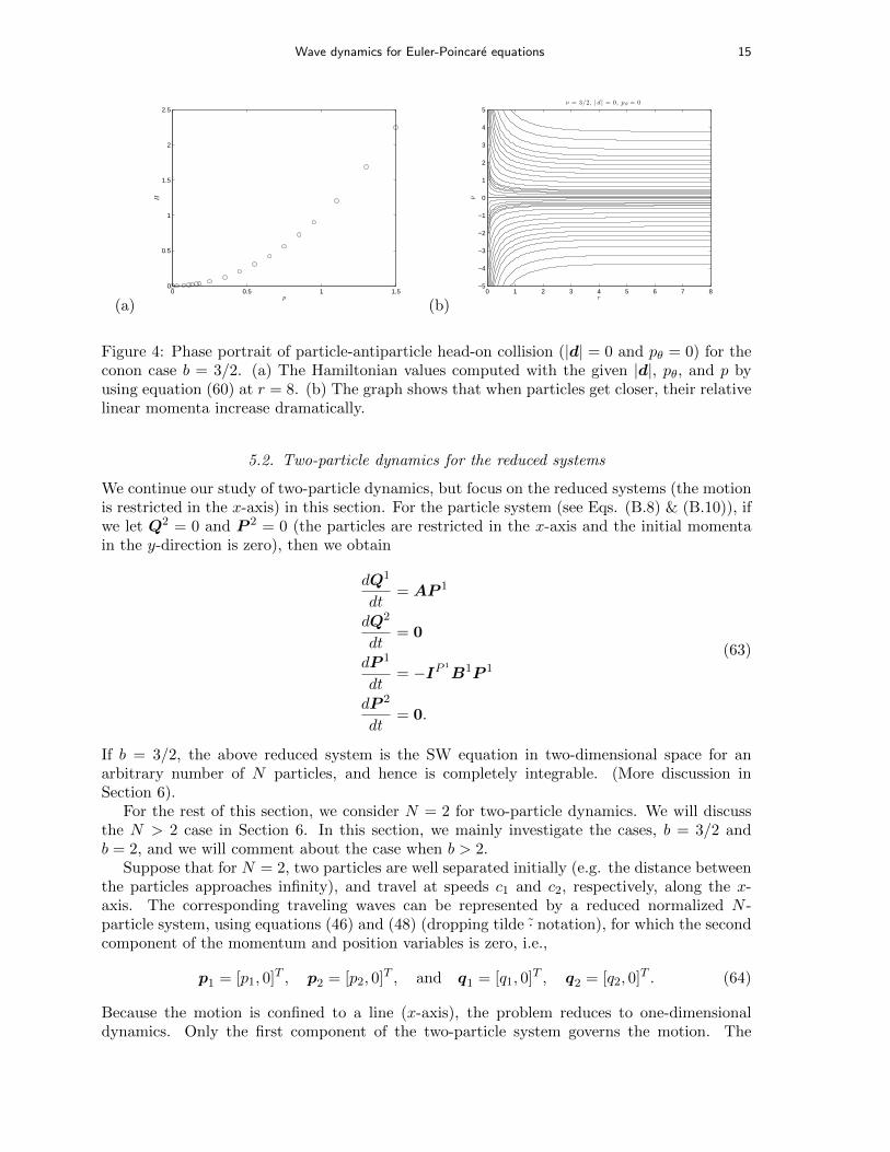
Figure 4 is the phase portrait for the particle-antiparticle head-on collision (|d| = 0 andpθ = 0). The graph shows that when particles get closer their relative linear momentumincreases dramatically. There is, however, no information revealed in the phase portrait aboutwhat happens to the linear momentum when r ≥ 0. We note that the particle motion in Figure3-4 is confined to a line due to the zero angular momentum. Moreover, the scattering orbitsin Figure 3 suggest that the relative linear momentum p changes sign at p = 0 for the casewhen the sum of linear momenta is non-zero, whereas the lack of scattering orbits in Figure4 indicates that the relative linear momentum p can only change sign passing through infinityin the particle-antiparticle head-on collision case (the sum of linear momenta is zero).

(a)0 0.5 1 1.5

0

0.5

1

1.5

2

2.5

p

H

(b)0 1 2 3 4 5 6 7 8

−5

−4

−3

−2

−1

0

1

2

3

4

5

r

pν = 3/2, |d | = 1, p θ = 0

Figure 3: Phase portrait for |d| = 1, pθ = 0 for b = 3/2. (a) The Hamiltonian values computedwith the given |d|, pθ, and p by using equation (60) at r = 8. (b) Three principle behaviorsare exhibited in the phase portrait for the two-particle interaction. The ejection orbits are inthe upper-half plane, whereas the capturing orbits are in the lower-half plane. The scatteringorbits are in the middle.

This behavior is similar to that exhibited by the one-dimensional SW equation, where theHamiltonian is not conserved when the support of a peakon and an antipeakon coincide ina head-on collision. This leads to divergence of the momenta in the limit to the collisiontime [7]. Similarly, for the N -particle system in this paper, equation (58) suggests that in aparticle-antiparticle head-on collision, when the peaks overlap, the Hamiltonian becomes

H =1

2|d|Gb−1(0). (62)

Since d = 0, we have H = 0 if d is zero initially. This would lead to blow-up of the linearmomentum as r → 0. As mentioned in the beginning of this section, the continuation of thesolutions can be achieved by imposing a conservation a law such as that of the Hamiltonian.The phase portrait analysis for b = 2, we refer readers to the results in reference [2].

Wave dynamics for Euler-Poincare equations 15

(a)0 0.5 1 1.5

0

0.5

1

1.5

2

2.5

p

H

(b)0 1 2 3 4 5 6 7 8

−5

−4

−3

−2

−1

0

1

2

3

4

5

r

p

ν = 3/2, |d | = 0, p θ = 0

Figure 4: Phase portrait of particle-antiparticle head-on collision (|d| = 0 and pθ = 0) for theconon case b = 3/2. (a) The Hamiltonian values computed with the given |d|, pθ, and p byusing equation (60) at r = 8. (b) The graph shows that when particles get closer, their relativelinear momenta increase dramatically.

5.2. Two-particle dynamics for the reduced systems

We continue our study of two-particle dynamics, but focus on the reduced systems (the motionis restricted in the x-axis) in this section. For the particle system (see Eqs. (B.8) & (B.10)), ifwe let Q2 = 0 and P 2 = 0 (the particles are restricted in the x-axis and the initial momentain the y-direction is zero), then we obtain

dQ1

dt= AP 1

dQ2

dt= 0

dP 1

dt= −IP 1

B1P 1

dP 2

dt= 0.

(63)

If b = 3/2, the above reduced system is the SW equation in two-dimensional space for anarbitrary number of N particles, and hence is completely integrable. (More discussion inSection 6).

For the rest of this section, we consider N = 2 for two-particle dynamics. We will discussthe N > 2 case in Section 6. In this section, we mainly investigate the cases, b = 3/2 andb = 2, and we will comment about the case when b > 2.

Suppose that for N = 2, two particles are well separated initially (e.g. the distance betweenthe particles approaches infinity), and travel at speeds c1 and c2, respectively, along the x-axis. The corresponding traveling waves can be represented by a reduced normalized N -particle system, using equations (46) and (48) (dropping tilde · notation), for which the secondcomponent of the momentum and position variables is zero, i.e.,

p1 = [p1, 0]T , p2 = [p2, 0]T , and q1 = [q1, 0]T , q2 = [q2, 0]T . (64)

Because the motion is confined to a line (x-axis), the problem reduces to one-dimensionaldynamics. Only the first component of the two-particle system governs the motion. The

16

system of ODEs for the first component of the two-particle system is

dq1

dt= Gb−1(0)p1 +Gb−1(|q1 − q2|)p2,

dq2

dt= Gb−1(|q2 − q1|)p1 +Gb−1(0)p2,

dp1

dt= −p1p2G

′b−1(|q1 − q2|)

q1 − q2

|q1 − q2|,

dp2

dt= −p1p2G

′b−1(|q2 − q1|)

q2 − q1

|q2 − q1|.

(65)

Introducing the sum and difference variables

P = p1 + p2, Q = q1 + q2

p = p1 − p2, q = q1 − q2,(66)

we obtain a system of ODEs for q and p

q = (Gb−1(0)−Gb−1(|q|)) p;

p =p2 − P 2

2G′b−1(|q|).

(67)

The direction field of equation (67) with P = 1 is shown in Figure 5, where (a) is the caseb = 3/2, and (b) corresponds to b = 2. It can be seen that the phase dynamics described inFigure 5(a) is the same as that of Figure 4(b) for the same setup and parameters. Figure 5,however, clearly shows the ejection, capture, and scattering behaviors indicated in [2].

(a)0 2 4 6 8 10

-6

-4

-2

0

2

4

6

q (b)0 2 4 6 8 10

-6

-4

-2

0

2

4

6

q

Figure 5: The direction field of equation (67) with P = 1. (a) b = 3/2. (b) b = 2. The graphsclearly show the ejection, capture, and scattering orbits for both b = 3/2 and b = 2.

Next, we consider the head-on collision case, for which P = 0. The direction fields shown inFigure 6 indicate that there are no scattering orbits, only ejection and capture orbits exist forhead-on collision for both b = 3/2 and b = 2 cases. This is consistent with the phase portraitin Figure 3(b) and those illustrated in [2].

As mentioned earlier, the lack of of scattering orbits implies that p can only change signthrough infinity in the case of particle-antiparticle head-on collision. To investigate further thedynamics of head-on collisions, we recall the Hamiltonian (58) for the motion of two particles

Wave dynamics for Euler-Poincare equations 17

(a)0 2 4 6 8 10

-6

-4

-2

0

2

4

6

q (b)0 2 4 6 8 10

-6

-4

-2

0

2

4

6

q

Figure 6: The direction field of equation (67) with P = 0 (head-on collision). (a) b = 3/2. (b)b = 2. The graphs show that there are no scattering orbits, only ejection and capture orbitsfor both b = 3/2 and b = 2.

confined to a line

H =1

4

(P 2 − p2

)Gb−1(q) +

1

4

(P 2 + p2

)Gb−1(0). (68)

For a particle-antiparticle head-on collision, P = 0 and we have

(Gb−1(0)−Gb−1(q)) =4H

p2. (69)

Using the above relation allows to rewrite equation (67) as

q = 4Hz, (70)

z = −1

2G′b−1(q), (71)

where z =1

p. Let Y = [q, z]T . The above equations represent a nonlinear autonomous system

Y = F (Y ). Since the radial derivative of Gb−1 vanishes at q = 0, due to the symmetry, Y (0)is a fixed-point. For smooth enough particles (Gb−1 ∈ C2, b ≥ 3), it is straightforward to showthat the eigenvalues of the Jacobian matrix for the system (70)-(71), linearized around thefixed-point, are real,

λ1,2 = ±√−2HG′′b−1(0). (72)

Hence the fixed-point Y (0) is locally a saddle, since G′′b−1(0) < 0 for b ≥ 3 and H > 0.From the Lyapunov function computed in Appendix C, we know that for particle-

antiparticle head-on collisions with b ≥ 3, once the motion of the particles is confined tothe x-axis, the solution stays on the stable manifold. Hence there are no scattering orbits andthe particles capture each other. We conclude that if the solitary waves are smooth enough(b ≥ 3), for particle-antiparticle collision, scattering orbits can only exist when the motion ofthe particles is not confined to a line, or the relative angular momentum is non-zero.

The property of non-uniqueness may allow scattering solutions for particle-antiparticle col-lision, even when the motion of particles is restricted to a line. A typical scattering solution isshown in Figure 7. In the figure, the resonance period (q = 0) is between t = 40 and t = 80.

18

(a)0 20 40 60 80 100 120

0

1

2

3

4

5

6

7

8

9

10

t

q

(b)0 20 40 60 80 100 120

−4

−3

−2

−1

0

1

2

3

4

t

1/p

Figure 7: A typical scattering solution of two-particle collision for b = 2. (a) The plot of q vst. (b) The plot of z vs t.

In general, our numerical experiments show that the length of resonance can be arbitrary (dueto the non-uniqueness of solutions). Figure 7 is the numerical integration for the two-particlecollision. The figure shows that after the resonance period the particles could exchange mo-menta as in collisions of two elastic bodies, and move away from each other. Nevertheless,particles are also allowed to keep their momenta, and these solutions allow q to become nega-tive after a resonance period. Figure 7 is generated by solving equations (70) and (71) usingthe sixth-order Runge-Kutta method developed in [20]. The initial conditions are z(0) = πand q(0) = 10. The time step is ∆t = 3.125e-5.

Finally, we focus on the choice b = 3/2, for which the derivative of the Green function Gb−1

is not continuous at q = 0. Hence, in a neighborhood of E containing Y (0), the solution mayor may not exist. One can enforce a continuation rule for solutions of the particle-antiparticlehead-on collision. In particular, this rule can be assigned to correspond to elastic collisions.i.e., the particles exchange momenta and scatter after the collision. We take a closer look atsuch solutions next.

5.3. Exact solution for b = 3/2

For the special case b = 3/2, we write the system of equations (65) in terms of the sum anddifference variables (66) as

P = 0, Q = (Gb−1(0) +Gb−1(|q|)P,

p = −1

2

(P 2 − p2

)sgn(q)G′b−1(|q|), q = (Gb−1(0)−Gb−1(|q|) p,

(73)

where sgn(q) is the signum function. The second pair in the above equations is the same asequations (67), since the Green functions for the elliptic equations are evenly symmetric. Weconsider the case of b = 3/2, for which the normalized Green function and its derivative are

G1/2(r) = e−r, G1/2(0) = 1, and G′1/2(r) = −e−r. (74)

Thus for this special case equation(73) becomes

P = 0, Q =(

1 + e−|q|)P,

p =1

2

(P 2 − p2

)sgn(q)e−|q|, q =

(1− e−|q|

)p.

(75)

Wave dynamics for Euler-Poincare equations 19

The above reduced system is a two-dimensional 2-body collision problem restricted to the x-axis. We note that these equations coincide with those for the interaction of two solitons of theone-dimensional SW equation [7]. (The exact solution of the above system was derived in [6]and [7].) In Appendix D, we present an example of the exact solution and use this to test thenumerical solution of equations (70)-(71).

5.4. Examples of particle interaction

We present numerical integration for the ODEs system to illustrate two-particle interaction.W focus on the special case b = 3/2.

Example 1: We first show the particle-antiparticle head-on collision for b = 3/2. Fromthe discussion above, the integration of the two-particle system suffers from divergence ofthe momentum when the two particles collide. Thus solutions are not defined at and afterthe collision. Because this example is a two-dimensional analogue of the one-dimensionalsoliton-antisoliton collision of the SW equation, we use this example to illustrate that forthe conically-shaped kernel (b = 3/2) the motion of the related two-dimensional waves canbecome completely integrable under appropriate initial data. This reduction projects the two-dimensional system to the one-dimensional completely integrable SW equation, while retainingthe full dependence on two spatial dimensions for the single channel solutions. To this end,we reconstruct the solution u by using the exact solutions of p and q obtained by equation(D.25), and the reconstruction formula (45). Suppose that initially the particle p1 = [2, 0]T islocated at q1 = [−8, 0]T , while the antiparticle p2 = [−2, 0]T is located at q2 = [8, 0]T . Fromequation (D.26), the two particles collide at tc ≈ 4.346573576213. Figure 8 is the plots of thefirst component of u before and after the collision at (a) t = 0, (b) t = 3.8, (c) t = 5.1 and (d)t = 7.9, respectively.

Example 2: We consider the case of two solitary waves travelling in the same direction.Suppose the solitary wave that has a larger amplitude (momentum) is behind and travels fasterthan the other one. The fast solitary wave will overcome the slow one, and after separating twosolitary waves will emerge which continue to travel at their original speeds. From Figure 3, forb = 3/2, if the sum of momenta is 1, there exist scattering orbits for relative momenta p ≤ 0.5.Because the momentum does not blow up when the two waves collide, the plots are obtainedby numerical integration of the 2-particle sysetm, equations (46) & (48). We choose the initialdata as p1 = [0.7, 0]T , q1 = [−22, 0]T , p2 = [0.3, 0]T , and q2 = [−10, 0]T , respectively, so thatthe sum of momenta is 1 and the relative momentum is 0.4. The time step for the integrationis ∆t = 1.0e-5. Figure 9 shows the simulation for the waves before, during, and after theovertaking process.

6. Initial data p1(x) = a sech2(x) for the reduced systems

6.1. Dispersionless case κ = 0

In this section, we investigate the reduced system (63) for N > 2 and b = 3/2. The normalizedGreen function is provided by equation (74). Suppose that we place N particles on the x-axiswith non-zero first momentum-component while setting the second component of momentumto zero. Suppose all other particles in the domain have zero momenta for both components.

20

(a) (b)

(c) (d)

Figure 8: Numerical reconstruction of the first-component of u for head-on collision betweenparticle and antiparticle for b = 3/2. The first component of u is shown at (a) t = 0, (b)t = 3.8, (c) t = 5.1, and (d) t = 7.9, respectively. Initially the particle p1 = [2, 0]T islocated at q1 = [−8, 0]T , while the antiparticle p2 = [−2, 0]T is located at q2 = [8, 0]T . (Theparticle locations and momenta are computed by using equation (D.25), as shown in Figure 1in Appendix D.

Then the first component of the particle system of equation (35) reduces to

qi =

N∑j=1

e−|qi−qj |pj ,

pi = −N∑j=1j 6=i

sgn(qi − qj)e−|qi−qj |pipj ,(76)

where i = 1, · · · , N . Here qi is the first coordinate of the ith particle on the x-axis, while piis its momentum. Equation (76) is a completely integrable system. It shares the same formand hence the same properties as that of the completely integrable N -particle system for theone-dimensional (1-D) SW equation studied in [16,21,22]. To illustrate that in two-dimensionalspace the solution behaviors, based on the setup and system (76), are the same as those of the1-D SW equation, we consider the following initial data. A 100 × 100 particle grid is placedin a domain of size [−20, 20]× [−20, 20]. Along the x-axis, the first-component momentum forthe particles is given by p(x) = 1

2sech2(x). The first momentum-component is zero outside thex-axis, whereas the second momentum-component is zero everywhere. This initial condition

Wave dynamics for Euler-Poincare equations 21

(a) (b)

(c) (d)

Figure 9: Numerical integration for the two-particle system for b = 3/2. Plots show the firstcomponent of u. (a) t = 0, (b) t = 23, (c) t = 35, (d) t = 60. The fast particle overtakes andthen leave the slow one. The initial conditions are p1 = [0.7, 0]T , q1 = [−22, 0]T , p2 = [0.3, 0]T ,and q2 = [−10, 0]T , respectively. From Figure 3, scattering orbits exist for these initial data.Plots are conducted by integrating the N -particle algorithm, (46) & (48). The time step is∆t = 1.0e-4.

is chosen to emulate the sharp traveling wave solution of the SW equation. The initial wavehump sharpens as it moves to the right, followed by others emerging humps from the initialcondition support.

Figure 10(a) shows the initial first-component of u, and (b) shows u at t = 12. Figure 11is a frontal view of Figure 10. The view direction is perpendicular to the x-axis. The figureshows that the slice along the x-axis is a smooth hump initially. Similar to the 1-D case, theinitial hump sharpens as it moves to the right, followed by another hump which emerges fromthe location of the initial condition. Figure 12 is another frontal view of Figure 10. The viewdirection is perpendicular to the y-axis. From this view direction, the waves look the same asthe conons, for which the radial derivative has a finite jump.

We remark that simulations in this section use the full two-dimensional N -particle algorithm(35) at the expense of computational cost. The number of particles in the calculation isN = 1280 (320 particle on each slice in the x-direction and 4 particles on the slice in they-direction initially; compared with 1000 particles in the 1-D simulation in [16]). That is whythe second emerging wave shown in Figures 10 and 11 displays a saw-tooth-like roughness. Amuch less expensive way to obtain a high-resolution result would be to compute the particleevolution on the x-axis only, i.e., evolve the q’s and p’s in equation (76), and then reconstruct

22

(a) (b)

Figure 10: Simulations for the completely integrable system (76), κ = 0. Numerical param-eters as in Figure 9. (a) Initial first-component of u. (b) First-component of u at t = 12.The initial data have non-zero first-component momenta along the x-axis and zero second-component momenta everywhere. The non-zero momenta along x-axis are distributed by12sech2(x).

the field u onto the whole two-dimensional plane by using equation (32) with the evolved q’sand p’s. Of course, in this manner we would not provide a full two-dimensional test of thenumerics but rather use the analytical reduction to one dimensional settings.

6.2. Dispersive case κ 6= 0

In this section we demonstrate the effect of taking κ 6= 0, i.e., of considering the dispersivedeformation.

As noted in Section 2.2, the dispersion relation is non-trivial in the dispersive deformation.It depends on both amplitude and direction of the constant parameter κ. Unlike its one-dimensional counterpart, this may have consequences in considering the limit κ → 0 as apossible dispersive regularization mechanism to handle non-smooth kernels.

In our numerical experiments, the initial condition for the first component of p is specifiedby p(x) = sech2(x) along the x-axis, and zero everywhere else, while the second component ofp is zero everywhere, for the finite dimensional dynamical system (30), corresponding to thedispersive PDE (22). However, unlike the previous non-dispersive example where κ = 0, wecarry out our numerical simulations by using equation (30) directly, without absorbing dx dyinto the p variable. Furthermore, we use the original Green functions without normalization.Similar to the example for κ = 0, the special case b = 3/2 is considered. Figure 13(a) showsthe initial data. Let the dispersive (constant) vector be denoted by κ = (κ1, κ2). Figure 13(b)shows the first-component of u, evolving from the initial data in Figure 13(a) to the final timet = 3 with the dispersive vector κ = (1, 0). The computational domain is [−20, 20] × [−5, 5]for p and q. The mesh size is dx = dy = 0.2. The temporal step size is ∆t = 0.1. Thefield u is reconstructed on the domain [−20, 20]× [−20, 20]. Figure14(a) shows that along thex-axis the initial data evolve into a front advancing from left to right followed by an oscillatorywave train, similar to the example observed in [21] for the nonlinear SW equation. Further,in analogy with Figures 13 and 14, Figure 15 shows the numerical experiments for κ = (1, 1)(left panel) and κ = (0, 1) (right panel), respectively. The development of oscillatory wavetrains are observed in all directions, as expected when both κ1 and κ2 are nonzero.

Wave dynamics for Euler-Poincare equations 23

(a) (b)

Figure 11: A frontal view of Figure 10. The view direction is perpendicular to the x-axis. Theinitial smooth hump is sharpening as it moves to the right, followed by another hump emergingfrom the location of the initial hump. First-component of u at t = 0, (a), and at t = 12, (b).

(a) (b)

Figure 12: A frontal view of Figure 10. The view direction is perpendicular to the y-axis.From this direction, the waves look the same as the conical solitary waves, for which the radialderivative has a finite jump. First-component of u at t = 0, (a), and at t = 12, (b).

7. Smooth initial data

Just as the particle algorithms developed for the SW equation [16,21–24], the N -particle systemin this paper can be seen as a Lagrangian numerical algorithm for solving the model PDEs (2).The peakon of the particle method for the SW equation behaves like a member of a functionalbasis. This basis is advantageous not only for approximating rough initial data, but smoothdata [16] can also be handled relatively well. This feature extends to the two-dimensionalsetting. In this section, we present an example with smooth initial data and follow numericallythe ensuing solutions. We show that the N -particle algorithm can be used as a numericalmethod for solving the model PDEs (2) in alternative to the traditional Eulerian methods forsmooth solutions, if certain technical issues, such as the computational cost, can be overcome.

In Section 7.1, we introduce an operator-splitting pseudospectral algorithm. The methodis called operator-splitting, because two sets of equations, one elliptic and one hyperbolic,are solved in alternating steps, as opposed to solving directly a non-local integral-differentialequation for the evolution of m. This operator-splitting method is introduced to assess the

24

(a) (b)

Figure 13: Same as Figure 11, but for the dispersive system (22) with κ 6= 0. (a) Initialfirst-component of u. (b) First component of u at t = 3. The initial data have non-zero first-component momenta along the x-axis and zero second-component momenta everywhere. Thenon-zero momenta along x-axis are distributed by sech2(x). The dispersive vector is κ = (1, 0).

(a) (b)

Figure 14: Frontal views of Figure 13(b). (a) View direction perpendicular to the x-axis. (b)View direction perpendicular to the y-axis.

particle algorithm for handling smooth solution. In Section 6, we have shown that the particlemethod is suitable for solutions with jump-derivatives at the peaks or with sharpening peaks.In Section 7.1, we introduce the pseudospectral method to compare with the particle algorithm,in particular for problems with smooth initial data and smooth solutions at later times. Weare interested in knowing how well the smooth solutions can be represented by a finite numberof particles when particles cluster at some places and coarsen at the others, because in [23], weshowed that for the one-dimensional case, particle clustering might induce instability for thealgorithm and cause blow-up, while particle coarsening would cause saw-tooth-like roughnessfor smooth solutions.

We remark that since the operator-splitting approach solves two sets of equations in alter-nating steps, the convergence property of the method to the true solution is a rather delicateproblem, due to the splitting error. Even in the one-dimensional case [25–28], the methodis not guaranteed to converge (although numerical convergences are established for both oneand two dimensional algorithms). Nevertheless, the primary advantage for introducing theoperator-splitting methods is to avoid solving a non-local integral-differential equation. The

Wave dynamics for Euler-Poincare equations 25

convergence and the error bound for the operator splitting are interesting open questions ontheir own right, even for the one-dimensional case, and thus belongs to a dedicated study anda paper.

7.1. An operator-splitting pseudospectral method for the model system (2)

The two-dimensional version of equations (2), for which x = (x, y)T , u = (u1, u2)T , andm = (m1,m2)T , in component form is

∂m1

∂t+ (u1)xm1 + (u2)xm2 + u1(m1)x + u2(m1)y +m1((u1)x + (u2)y) = 0,

∂m2

∂t+ (u1)ym1 + (u2)ym2 + u1(m2)x + u2(m2)y +m2((u1)x + (u2)y) = 0.

(77)

After collecting terms of the above equations, together with equation (5), we obtain

∂m1

∂t+ (u1m1)x + (u2m1)y +m1(u1)x +m2(u2)x = 0,

∂m2

∂t+ (u1m2)x + (u2m2)y +m1(u1)y +m2(u2)y = 0,

(78)

where

m1 =(1− a2(∂xx + ∂yy)

)bu1,

m2 =(1− a2(∂xx + ∂yy)

)bu2.

(79)

We propose an operator-splitting pseudospsectral method for solving the equations (2) byalternating between solving equations (78) and (79). In detail, the resulting algorithm consistsof the following steps:

Step 1. Given smooth initial data u01 and u0

2, we compute m01 and m0

2 by using equation (6).

Step 2. Integrate equation (78) by using the two-stage, second-order Runge-Kutta method(53). All derivatives are computed by the pseudospectral method. For example, the jth row ofthe partial derivative of u1m1 with respect to x is computed by

[(u1m1)x]j = F−1 {ikxF {[u1m1]j}} , (80)

where F is the one-dimensional Fast Fourier Transform, F−1 is the inverse Fast Fourier Trans-form, kx is the corresponding wavenumbers, and i =

√−1.

Step 3. After the integration over ∆t in Step 2, obtain m11 and m1

2. Compute u11 and u1

2 byusing equation (6) again.

Step 4. Return to Step 2 and Step 3 for computing mn1 , mn

2 , un1 , and un2 , where n = 2, 3, . . . .

We remark that the proposed algorithm is a two-dimensional extension of the operator-splittingalgorithms developed for the SW equation [27,28]. Similar to those one-dimensional solvers, animplicit iteration between equation (78) and (79) can be implemented for the current algorithmto guarantee the convergence of numerical solutions.

We now are now in position to integrate the equations (2) for smooth initial condition.Consider the smooth initial data u = (u1, u2)T , where

26

u1(x, y) = sech

(x2 + y2

4

),

u2(x, y) = 0.

(81)

Figure 17(a) and (b) are simulations for u1 and u2 at t = 3, respectively. The operator-splittingpseudospectral method is used with dx = dy = 0.125 and ∆t = 0.0125. The computationaldomain is [−32, 32]× [−32, 32]. b = 3/2 for the simulations. Figure 18(a) and (b) are the samesimulations as Figure 17(a) and (b), but are obtained by using the N -particle algorithm with51×51 particles placed in a 16×16 domain initially. The time step is ∆t = 0.1 for the particlealgorithm. The velocities are reconstructed on a 32× 32 domain with dx = dy = 0.16. Figure17 and Figure 18 are virtually indistinguishable. The difference between Figure 17 and Figure18, for both components in the maximum norm, is at the order of O(10−3). We remark thatfor all simulations in this section we use the N -particle algorithm defined in equation (35), forwhich the Green function is not normalized for convenience of comparison.

Figures 19 and 20 depict the result of simulations at t = 5 for the same initial data (81), ob-tained by the pseudospectral and N -particle algorithms, respectively. The number of particlesis 81×81, the same as that for the simulations at t = 3. At first glance, Figures 19 and 20 seemidentical. However, if we blow up the region around the peak of u1 in Figure 20(a), we candetect a saw-tooth-like roughness. This is because many particles have moved away from thisregion at this time, and the smooth wave cannot be represented by too few “conon”-particles.When we increase the particle number from 81 × 81 to 101 × 101, this saw-tooth roughnessbecomes less visible, as shown in Figure 21. However, with the increment of particles from 81to 101 in one direction, the computational cost increases about six-fold. This is because thecost of double summation is O(N2) (with N the number of particles), and we reduce the tem-poral step size to a half to maintain the stability of the two-stage RK scheme. Together withoverhead, the elapsed CPU-time for the 101× 101 mesh grid is 6 times more than the 81× 81one. Therefore, long-time simulations for this example by using the N -particle algorithm arenot feasible without introducing a fast algorithm, such as the fast multipole method, or bytaking advantage of massive parallelization. This is beyond the current scopes of the paper.Nevertheless, developing fast algorithms for the N -particle method can be implemented andwe expect to report on this in the near future. Before ending this section, we demonstrate theability of handling smooth data for the operator-splitting pseudospectral method. We evolvethe initial data (81) until t = 20. Figure 22(a) and (b) show the result of these algorithmsimulations for u1 and u2, respectively.

8. Discussion and concluding remarks

In this paper, we have studied a class of multidimensional PDEs for a parametric family ofelliptic operators, and extended the class to a dispersive deformation which, to the best ofour knowledge, has not been investigated in the literature. We have used the Lagrangianformulation as the most natural avenue for deriving finite-dimensional particle systems dis-cretizing the PDE system. These particle systems for non-smooth kernels (Green functions) ofthe invertible elliptic operator govern nontrivial dynamics worth examining in further detail.Within the class we have focussed on, the regularity of the Green functions is determined bythe power of the elliptic operator, which we denoted by b. If b = 3/2, the Green function hasa finite jump in its radial derivative reminiscent of the peakon solution for the SW equation.In fact, by using this “conon” case, in which the motion of the two-dimensional particles isrestricted in a one-dimensional channel, we show that this choice of non-smooth kernel reduces

Wave dynamics for Euler-Poincare equations 27

the two-dimensional particle system to the completely integrable one-dimensional case, eventhough the “single channel” solution retains its dependence on two spatial dimensions. Withthis reduction, complete intergrability persists for the dispersive deformation, giving rise totraveling wave solutions which are smooth along their direction of travel.

We have also studied particle collisions restricted to a line for various parameters b of theGreen function kernel (5). We have found that for sufficiently smooth kernels, when b ≥ 3, twoparticles head-on collisions in finite time are avoided. This is in contrast to their less-smoothcounterparts with b < 3.

A pseudospectral scheme for solving the PDEs under study was introduced to provide anindependent means of numerically computing smooth solutions of the PDE’s we studied. Bycomparing solutions obtained with this scheme with those from the N -particle algorithm, weshow that the N -particle system can potentially be used as a Lagrangian method for solvingthe model PDEs, in particular when weak solutions are considered. Nevertheless, for longtime simulations and smooth initial data, it is clearly necessary to develop fast summationalgorithms for the N -particle to achieve realistic computational costs.

We do not investigate particle dynamics for b ≤ 1 in this paper. Since the Green functionof the elliptic operator corresponding to this power is unbounded at the support point, itwould be necessary to regularize these kernels to implement an N -particle algorithm. Theregularization results in a smooth modified kernel. In principle, the behavior of the regularizedGreen function should in principle be similar to that of this function with a parameter b inthe range b ≥ 3. We leave this to future work. Also left to forthcoming investigations arethe implications of the sensitivity to the singularity of the Green functions for image matchingapplications, and the convergence of the point particle approximation to solutions of the modelPDEs under various singular kernels.

Finally, we remark that the flexibility in the choice of elliptic operators connecting the“primary” field u and the “auxiliary” field m could be exploited to move beyond the realmof interesting mathematical PDE’s and towards more physically grounded models such as theEuler equations for ideal fluids [29, 30]. Doing so could provide valid alternatives to vortexmethods for numerical simulations of 2D and 3D Euler equations, as well as analytical toolswhich may prove useful in theoretical investigations of these equations.

9. Acknowledgements

RC acknowledges the support of NSF DMS-0509423, CMG-0620687, DMS-0908423, DMS-1009750, and RTG DMS-0943851.

Appendix A. Lagrangian and Eulerian formulations

Suppose that J(ξ, t) is the Jacobian determinant of the diffeomorphism x = q(ξ, t)parametrized by time t,

J(ξ, t) ≡ det

(∂xi∂ξj

).

The conjugate field p(ξ, t) is defined by

m(q(ξ, t), t

)≡ p(ξ, t)

J(ξ, t). (A.1)

28

The Yukawa operator L gives

m = Lu , or u = G ∗m.

Let y = q(η, t). We have

u =dq

dt=Gb−n/2 ∗m

=

∫RnGb−n/2

(|x− y)|

)m(y, t) dy

=

∫RnGb−n/2

(|q(ξ, t)− q(η, t)|

)m(q(η, t), t) dq(η, t)

=

∫RnGb−n/2

(|q(ξ, t)− q(η, t)|

)p(η, t) dVη.

(A.2)

We now show that if we define

dp

dt= −

∫RnG′b−n/2

(|q(ξ, t)− q(η, t)|

) q(ξ, t)− q(η, t)

|q(ξ, t)− q(η, t)| p(ξ, t) · p(η, t) dVη ,

we recover the model PDEs (2). To this end, we follow the diffeomorphism variable transfor-mation to compute

dp

dt=−

∫RnG′b−n/2

(|q(ξ, t)− q(η, t)|

) q(ξ, t)− q(η, t)

|q(ξ, t)− q(η, t)| p(ξ, t) · p(η, t) dVη

=−∫RnG′b−n/2

(|x− y|

) x− y|x− y|J(ξ, t) m(x, t) ·m(y, t) dy

=−mj(x, t)∇x

∫RnGb−n/2

(|x− y|

)mj(y, t) dy J(ξ, t)

=−mj(x, t)∇xujJ(ξ, t)

=−m · (∇u)TJ(ξ, t).

(A.3)

On the other hand, by the definition of the conjugate field (A.1), we have

dp

dt=d

dt(m(q(ξ), t)J(ξ, t))

=d

dtm(q(ξ), t) J(ξ, t) +m(q(ξ), t)

dJ(ξ, t)

dt

=

(mt +

dq(ξ, t)

dt· ∇m(x, t)

)J(ξ, t) +m(∇ · u)

)J(ξ, t)

=(mt + (u · ∇)m+m(∇ · u)

)J(ξ, t).

(A.4)

Here we use the well known property of determinant differentiation (10). From equations (A.3)and (A.4) the Eulerian form of the model equations (2) follows.

Next, we derive the evolution equation of the determinant J(ξ, t) in equation (25). Fromthe determinant differentiation (10) and equation (A.2), we have

dJ

dt= J ∇ · u = J ∇ ·

∫R2

Gb−1

(|x− q(η, t)|

)p(η, t) dVη

= J

∫R2

G′b−1

(|x− q(η, t)|

)(x− q(η, t))· p(η, t)

|x− q(η, t)| dVη.

(A.5)

Wave dynamics for Euler-Poincare equations 29

If J is evaluated at x = q(ξ, t), then

dJ

dt= J

∫R2

G′b−1

(|q(ξ, t)− q(η, t)|

)(q(ξ, t)− q(η, t))· p(η, t)

|q(ξ, t)− q(η, t)| dVη. (A.6)

Appendix B. Notations for numerical implementation

For numerical implementation, we represent the N -particle systems in the following matrix-vector forms. Let

Qα =

qα1qα2...qαN

, P α =

pα1pα2...pαN

, (B.7)

The system of equations for Q can be written as

dQα

dt= AP α, α = 1, 2, (B.8)

where

A =

Gb−1(|q1 − q1|) Gb−1(|q1 − q2|) · · · Gb−1(|q1 − qN |)Gb−1(|q2 − q1|) Gb−1(|q2 − q2|) · · · Gb−1(|q2 − qN |)

......

. . ....

Gb−1(|qN − q1|) Gb−1(|qN − q2|) · · · Gb−1(|qN − qN |)

, (B.9)

while the system for P is

dP α

dt= −

[IP

1

BαP 1 + IP2

BαP 2], α = 1, 2, (B.10)

with

Bα =

0 G′b−1(|q1 − q2|) qα1−qα2

|q1−q2| · · · G′b−1(|q1 − qN |) qα1−qαN|q1−qN |

G′b−1(|q2 − q1|) qα2−qα1|q2−q1| 0 · · · G′b−1(|q2 − qN |) qα2−qαN

|q2−qN |...

.... . .

...

G′b−1(|qN − q1|) qαN−qα1|qN−q1| G′b−1(|qN − q2|) qαN−qα2

|qN−q2| · · · 0

,

(B.11)and

IP1

=

p1

1 0 · · · 00 p1

2 · · · 0...

.... . .

...0 0 · · · p1

N

, IP2

=

p2

1 0 · · · 00 p2

2 · · · 0...

.... . .

...0 0 · · · p2

N

. (B.12)

Appendix C. Lyapunov function and stable manifold

For b ≥ 3, the Lyapunov (energy) function for the system (70) & (71) that satisfies

dV

dt(q, z) = 0, (C.13)

30

is

V (q, z) = 2Hz2 +1

2Gb−1(q). (C.14)

The solution through the point (η1, η2) is given by the curve V (q, z) = V (η1, η2). The realcurves V (q, z) ≡ h, where h is some constant, are given by equations

z = ±√

2h−Gb−1(q)

4H, (C.15)

for all q for which 2h − Gb−1(q) ≥ 0. This implies that when h = V0 = V (0, 0) =1

2Gb−1(0),

the stable manifold is

z =

√Gb−1(0)−Gb−1(q)

4H. (C.16)

Here we simply recover equation (69). Moreover, for P = 0, equation (68) becomes

H(q, z) =1

4z2(Gb−1(0)−Gb−1(q)) , (C.17)

for any q and z. Substituting the above H into the Lyapunov function, we obtain

V (q, z) =1

2Gb−1(0) = V0, (C.18)

for any q and z.

Appendix D. Exact solution of the head-on collision

The Hamiltonian that generates the system (75) is

HA =1

2

(p2

1 + p22

)+ p1p2e

−|q1−q2| =1

2

(c2 + c2

)(D.19)

From equation (50), we have P (0) = c1 + c2 and p(0) = c1 − c2. Also, because initially thelocations of the two particles are [x1, 0] and [x2, 0], we have Q(0) = x1+x2 and q(0) = x1−x2 =γ is the initial distance between the two particles. Therefore, with these initial data, the initialvalue problems (75) can be solved. In particular, the second pair of equation (75) can be solvedby eliminating p in the q equation by noting that the Hamiltonian that generates equation(75)is

H =1

2P 2(

1 + e−|q|)

+1

2p2(

1− e−|q|)

= c21 + c2

2, (D.20)

and P (t) = c1 + c2. The solution of the second pair of equation (75) is shown in [7] and isequal to

q = − log

[4γ(c1 − c2)2e(c1−c2)t(

γe(c1−c2)t + 4c21

) (γe(c1−c2)t + 4c2

2

)] ,p = ±γ(c1 − c2)(e−(c1−c2)t − 4c1c2)

γe−(c1−c2)t + 4c1c2.

(D.21)

Wave dynamics for Euler-Poincare equations 31

The solutions of (D.21) for head-on collision (particle-antiparticle collision) has c1 = −c2 = cand thus can be simplified to

q = −2 log

[4c√γect

γe2ct + 4c2

],

p = ±2cγe−2ct + 4c2

γe−2ct − 4c2.

(D.22)

If we choose γ = 4c2, the particle-antiparticle collision occurs at time t = 0 at x = 0, and

q = −2 log sech(ct),

p = ± 2c

tanh(ct).

(D.23)

The constructed exact solution can be compared with numerical solution of equations (70)and (71). For b = 3/2, the Green function is G1/2(q) = e−|q|. Note that the radial derivativehas a finite jump and thus we write equations (70) and (71) as

q = 4Hz,

z =1

2sgn(q)e−|q|,

(D.24)

To compare the exact solution (D.23) with that obtained by solving equation (D.24), we shiftthe collision time to tc > 0 so that

q(t− tc) = −2 log sech(c(t− tc)),

p(t− tc) = ± 2c

tanh(c(t− tc)).

(D.25)

If we choose c = 2, the initial separation of the particles at t = 0 is 4c2 = 16, and the collisiontime tc satisfies

sech(2tc) = e−8, or tc =1

2sech−1(e−8) ≈ 4.346573576213. (D.26)

For this choice of c and tc, the initial relative momentum is

p(−tc) =4

tanh(−2tc)≈ −4. (D.27)

Hence the initial data for equation (D.24) are

q0 = 16, z0 = −1

4. (D.28)

Figure 1 compares the exact solutions (D.25) and the numerical solutions of equation (D.24)obtained by using the sixth-order Runge-Kutta method. Equation (D.28) is used as the initialdata and the time step is ∆t = 3.125e-05. The differences between the two calculations in2-norm, defined in (54), for q and z are 2.9506e-05 and 8.7397e-07, respectively.

References

1. M. F. Beg, M. I. Miller, A. Trouve, and L. Younes, Computing large deformation metric mappingsvia geodesics flows of diffeomorphisms, Int. J. Comp. Vis. 61:139–157 (2005).

2. R. McLachlan and S. Marsland, N-particle dynamics of the euler equations for planar diffeomorphisms,Dyn. Sys. 22:269–290 (2007).

32

3. D. D. Holm, J. T. Ratnanather, A. Trouve, and L. Younes, Soliton dynamics in computationalanatomy, Neuroimage 23:S170–S178 (2004).

4. M. Miller and L. Younes, Group actions, homeomorphisms, and matching: A general framework, In-ternational Journal of Computer Vision 41 (2001), no. 1/2.

5. S. Joshi and M. I. Miller, Landmark matching via large deformation diffeomorphisms, IEEE Trans.Image Processing 9:1357–1370 (2000).

6. R. Camassa and D. D. Holm, An integrable shallow water equation with peaked solitons, Phys. Rev.Lett. 71:1961–1964.

7. R. Camassa, D. D. Holm, and J. M. Hyman, A new integrable shallow water equation, Advan. Appl.Mech. 31:1–33 (1994).

8. S. Marsland and C. Twining, Constructing diffeomorphic representations for the groupwise analysis ofnon-rigid registrations of medical images, IEEE Transactions on Medical Imaging 23 (2004), no. 8.

9. M. Vaillant, M. I. Miller, L. Younes, and T. A., Statistics on diffeomorphisms via tangent spacerepresentations, NeuroImage 23:S161–S169 (2004).

10. M. Miller, A. Trouve, and L. Younes, On metrics and the euler-lagrange equations of computationalanatomy, Annual Reviews in Biomedical Engineering 4:375–405 (2002).

11. D. Mumford and A. Desolneux, Pattern Theory: The Stochastic Analysis of Real World Signals, A KPeters, Lid, Natick, MA, 2010.

12. D. Kuang and L. Lee, A feedback control geodesic landmark shooting algorithm for template matchingand pattern recognition, .

13. M. I. Miller, A. Trouve, and L. Younes, Geodesic shooting for computational anatomy, J Math Imaging24:209–228 (2006).

14. A. Chertock, P. Du Toit, and J. E. Marsden, Integration of the epdiff equation by particle methods,ESAIM:M2AN 46:515–534 (2012).

15. K. Mohseni, H. Zhao, and J. Marsden, Shock regularization for the burgers equation, AIAA Paper2006-1516, 44th AIAA Aerospace Science Meeting and Exhibit (2006), 9-12.

16. R. Camassa, J. Huang, and L. Lee, Integral and integrable algorithms for a nonlinear shallow-waterwave equation, J. Comput. Phys. 216:547–572.

17. M. Abramowitz and I. Stegun, Handbook of Mathematical Functions, Dover, 1965.18. L. Perko, Differential Equations and Dynamical Systems, 2nd ed., Springer-Verlag, New York, 1996.19. L. Landau and E. Lifshitz, Mechanics, 2nd ed., Pergamon,Oxford, 1969.20. J. C. Butcher, On runge-kutta processes of high order, J. Austral. Math. Soc. 4:179–194.21. R. Camassa, Characteristics and initial value problem of a completely integrable shallow water equation,

DCDS-B 3:115–139 (2003).22. R. Camassa and L. Lee, Complete integrable particle methods and the recurrence of initial states for a

nonlinear shallow-water wave equation, J. Comp. Phys. 227:7206–7221 (2008).23. R. Camassa, J. Huang, and L. Lee, On a completely integral numerical scheme for a nonlinear shallow-

water wave equation, J. Nonlin. Math. Phys. 12:146–162.24. R. Camassa and L. Lee, A completely integrable particle method for a nonlinear shallow-water wave

equation in periodic domains, DCDIS-A 14(S2):1–5 (2007).25. R. Camassa, P. Chiu, L. Lee, and T. Sheu, Viscous and inviscid regularizations in a class of evolutionary

partial differential equations, J. Comput. Phys. 229:6676–6687 (2010).26. R. Camassa, P. Chiu, L. Lee, and T. Sheu, A particle method and numerical investigation of a quasi-

linear partial differential equation, Comm. Pure and Appl. Math. (2011), 1503-1512.27. P. Chiu, L. Lee, and T. Sheu, A dispersion-relation-preserving algorithm for a nonlinear shallow-water

wave equation, J. Comput. Phys. 228:8034–8052 (2009).28. P. Chiu, L. Lee, and T. Sheu, A sixth-order dual preserving scheme for the sw equation., J. Comput.

Appl. Math. 223:2767–2778 (2010).29. D. Mumford and P. Michor, On euler’s equation and “epdiff”, J. Geom. Mech. 6 (2013), no. 3.30. C. J. Cotter, D. D. Holm, H. O. Jacobs, and D. M. Meier, A jetlet hierarchy for ideal fluid dynamics,

J. Phys. A: Math 47 (2014), no. 352001.

Department of Mathematics, University of North Carolina, Chapel Hill, USA, NC27599

Department of Mathematics, University of Wyoming, Laramie, USA, WY82071

Department of Mathematics, University of Wyoming, Laramie, USA, WY82071

Wave dynamics for Euler-Poincare equations 33

(a) (b)

Figure 15: Same as Figure 13 and 14 with different choices of κ. Left panel, (a), κ = (1, 1),and right panel, (b), κ = (0, 1). The final time is t = 3 for both (a) and (b). Top to bottomare first-component of u in two dimensions, with frontal view from x-axis, and frontal viewfrom y-axis.

34

(a) (b)

Figure 16: The initial conditions for the comparison between particle and operator-splittingalgorithms. (a) First component u1(x, y) = sech

((x2 + y2)/4

). (b) Second component

u2(x, y) = 0.

(a) (b)

Figure 17: Simulations for the initial data shown in Figure 16 at t = 3, by using the operator-splitting pseudospectral method, conical case b = 3/2, with dx = dy = 0.125 and ∆t = 0.0125.The computational domain is [−16, 16]× [−16, 16]. (a) The first component u1. (b) The secondcomponent u2.

Wave dynamics for Euler-Poincare equations 35

(a) (b)

Figure 18: Same as Figure 17, but by using the N -particle algorithm with 81 × 81 particlesplaced in a [−8, 8] × [−8, 8] domain initially. The time step is ∆t = 0.1. The velocities arereconstructed on a [−16, 16]× [−16, 16] domain with dx = dy = 0.1. (a) The first componentu1. (b) The second component u2. The difference between Figure 17 and Figure 18, for bothcomponents in the maximum norm, is at the order of O(10−3). The two figures are virtuallyidentical.

(a) (b)

Figure 19: Same as Figure 16 but t = 5, by using the operator-splitting pseudospectral method.b = 3/2 for the simulations. dx = dy = 0.25 and ∆t = 0.025. The computational domain is[−32, 32]× [−32, 32]. (a) The first component u1. (b) The second component u2.

36

(a) (b)

Figure 20: Same as Figure 19, by the N -particle algorithm with 81× 81 particles placed in a[−8, 8] × [−8, 8] domain initially. The time step is ∆t = 0.1. The velocities are reconstructedon a [−16, 16] × [−16, 16] domain with dx = dy = 0.1. (a) First component u1. (b) Secondcomponent u2. There is visible saw-tooth like roughness near the tip of the u1 wave.

(a) (b)

Figure 21: Same simulations as Figure 20, obtained by using the N -particle algorithm with101 × 101 particles placed in a [−8, 8] × [−8, 8] domain initially. The time step is ∆t = 0.1.The velocities are reconstructed on a [−16, 16] × [−16, 16] domain with dx = dy = 0.08. (a)The first component u1. (b) The second component u2. The tip of the u1 wave is smootherthan that in Figure 20.

Wave dynamics for Euler-Poincare equations 37

(a) (b)

Figure 22: Same as Figure 16 at t = 20, by using the operator-splitting pseudospectral method.b = 3/2 for the simulations. dx = dy = 0.25 and ∆t = 0.025. The computational domain is[−32, 32]× [−32, 32]. (a) The first component u1. (b) The second component u2.

(a)0 1 2 3 4 5 6 7 8 9

0

2

4

6

8

10

12

14

16

18

t

q

6th−order RKexact

(b)0 1 2 3 4 5 6 7 8 9

−0.4

−0.3

−0.2

−0.1

0

0.1

0.2

0.3

0.4

t

1/p

6th−order RKexact

Figure 1: Comparison between the exact solutions computed by equation (D.25) and thenumerical solutions of equation (D.24) obtained by using the sixth-order Runge-Kutta methodwith q0 = 16 & z0 = 1/4. The time step is ∆t = 3.125e-5. (a) The distance between theparticle and the antiparticle versus time. The difference in 2-norm between the exact solutionsand the numerical solutions is 2.9506e-05. (b) The (inverse) relative momentum versus time.The difference in 2-norm between the exact solutions and the numerical solutions is 8.7397e-07.