Solid State Theory

Spring Semester 2013

Manfred SigristInstitut fur Theoretische Physik HIT K23.8

Tel.: 044-633-2584Email: sigrist@itp.phys.ethz.ch

Website: http://www.itp.phys.ethz.ch/research/condmat/strong/

Lecture Website:http://www.itp.phys.ethz.ch/education/fs13/sst

Literature:

• N.W. Ashcroft and N.D. Mermin: Solid State Physics, HRW International Editions, 1976.

• C. Kittel: Einfuhrung in die Festkorperphysik, R. Oldenburg Verlag, 1983.

• C. Kittel: Quantentheorie der Festkorper, R. Oldenburg, 1970.

• O. Madelung: Introduction to solid-state theory, Springer 1981; auch in Deutsch in dreiBanden: Festkoperphysik I-III, Springer.

• J.M. Ziman: Principles of the Theory of Solids, Cambridge University Press, London,1972.

• M.P. Marder: Condensed Matter Physics, John Wiley & Sons, 2000.

• G. Grosso & G.P. Parravicini: Solid State Physics, Academic Press, 2000.

• G. Czychol: Theoretische Festkorperphysik, Springer 2004.

• P.L. Taylor & O. Heinonen, A Quantum Approach to Condensed Matter Physics, Cam-bridge Press 2002.

• G.D. Mahan, Condensed Matter in a Nutshell, Princeton University Press 2011.

• numerous specialized books.

1

Contents

Introduction 5

1 Electrons in the periodic crystal - band structure 81.1 Symmetries of crystals . . . . . . . . . . . . . . . . . . . . . . . . . . . . . . . . . 8

1.1.1 Space groups of crystals . . . . . . . . . . . . . . . . . . . . . . . . . . . . 81.1.2 Reciprocal lattice . . . . . . . . . . . . . . . . . . . . . . . . . . . . . . . . 10

1.2 Bloch’s theorem and Bloch functions . . . . . . . . . . . . . . . . . . . . . . . . . 111.3 Nearly free electron approximation . . . . . . . . . . . . . . . . . . . . . . . . . . 121.4 Tight-binding approximation . . . . . . . . . . . . . . . . . . . . . . . . . . . . . 15

1.4.1 Linear combination of atomic orbitals - LCAO . . . . . . . . . . . . . . . 151.4.2 Band structure of s-orbitals . . . . . . . . . . . . . . . . . . . . . . . . . . 161.4.3 Band structure of p-orbitals . . . . . . . . . . . . . . . . . . . . . . . . . . 171.4.4 Wannier functions . . . . . . . . . . . . . . . . . . . . . . . . . . . . . . . 191.4.5 Tight binding model in second quantization formulation . . . . . . . . . . 21

1.5 Symmetry properties of the band structure . . . . . . . . . . . . . . . . . . . . . 211.6 Band-filling and materials properties . . . . . . . . . . . . . . . . . . . . . . . . . 23

1.6.1 Electron count and band filling . . . . . . . . . . . . . . . . . . . . . . . . 241.6.2 Metals, semiconductors and insulators . . . . . . . . . . . . . . . . . . . . 24

1.7 Semi-classical description . . . . . . . . . . . . . . . . . . . . . . . . . . . . . . . 271.7.1 Equations of motion . . . . . . . . . . . . . . . . . . . . . . . . . . . . . . 271.7.2 Bloch oscillations . . . . . . . . . . . . . . . . . . . . . . . . . . . . . . . . 281.7.3 Current densities . . . . . . . . . . . . . . . . . . . . . . . . . . . . . . . . 28

2 Semiconductors 352.1 The band structure in group IV . . . . . . . . . . . . . . . . . . . . . . . . . . . . 36

2.1.1 Crystal and band structure . . . . . . . . . . . . . . . . . . . . . . . . . . 362.2 Elementary excitations . . . . . . . . . . . . . . . . . . . . . . . . . . . . . . . . . 38

2.2.1 Electron-hole excitations . . . . . . . . . . . . . . . . . . . . . . . . . . . . 392.2.2 Excitons . . . . . . . . . . . . . . . . . . . . . . . . . . . . . . . . . . . . . 402.2.3 Optical properties . . . . . . . . . . . . . . . . . . . . . . . . . . . . . . . 42

2.3 Doping semiconductors . . . . . . . . . . . . . . . . . . . . . . . . . . . . . . . . . 442.3.1 Impurity state . . . . . . . . . . . . . . . . . . . . . . . . . . . . . . . . . 442.3.2 Carrier concentration . . . . . . . . . . . . . . . . . . . . . . . . . . . . . 45

2.4 Semiconductor devices . . . . . . . . . . . . . . . . . . . . . . . . . . . . . . . . . 462.4.1 pn-contacts . . . . . . . . . . . . . . . . . . . . . . . . . . . . . . . . . . . 462.4.2 Diodes . . . . . . . . . . . . . . . . . . . . . . . . . . . . . . . . . . . . . . 472.4.3 MOSFET . . . . . . . . . . . . . . . . . . . . . . . . . . . . . . . . . . . . 48

3 Metals 513.1 The Jellium model . . . . . . . . . . . . . . . . . . . . . . . . . . . . . . . . . . . 51

3.1.1 Theory of metals - Sommerfeld and Pauli . . . . . . . . . . . . . . . . . . 523.1.2 Stability of metals - a Hartree-Fock approach . . . . . . . . . . . . . . . . 54

2

3.2 Charge excitations . . . . . . . . . . . . . . . . . . . . . . . . . . . . . . . . . . . 573.2.1 Dielectric response and Lindhard function . . . . . . . . . . . . . . . . . . 573.2.2 Electron-hole excitation . . . . . . . . . . . . . . . . . . . . . . . . . . . . 593.2.3 Collective excitation - Plasmon . . . . . . . . . . . . . . . . . . . . . . . . 603.2.4 Screening . . . . . . . . . . . . . . . . . . . . . . . . . . . . . . . . . . . . 62

3.3 Phonons . . . . . . . . . . . . . . . . . . . . . . . . . . . . . . . . . . . . . . . . . 663.3.1 Vibration of a isotropic continuous medium . . . . . . . . . . . . . . . . . 663.3.2 Phonons in metals . . . . . . . . . . . . . . . . . . . . . . . . . . . . . . . 683.3.3 Peierls instability in one dimension . . . . . . . . . . . . . . . . . . . . . . 693.3.4 Dynamics of phonons and the dielectric function . . . . . . . . . . . . . . 73

4 Itinerant electrons in a magnetic field 764.1 The de Haas-van Alphen effect . . . . . . . . . . . . . . . . . . . . . . . . . . . . 76

4.1.1 Landau levels . . . . . . . . . . . . . . . . . . . . . . . . . . . . . . . . . . 764.1.2 Oscillatory behavior of the magnetization . . . . . . . . . . . . . . . . . . 784.1.3 Onsager equation . . . . . . . . . . . . . . . . . . . . . . . . . . . . . . . . 79

4.2 Quantum Hall Effect . . . . . . . . . . . . . . . . . . . . . . . . . . . . . . . . . . 804.2.1 Hall effect of the two-dimensional electron gas . . . . . . . . . . . . . . . . 824.2.2 Integer Quantum Hall Effect . . . . . . . . . . . . . . . . . . . . . . . . . 834.2.3 Fractional Quantum Hall Effect . . . . . . . . . . . . . . . . . . . . . . . . 89

5 Landau’s Theory of Fermi Liquids 935.1 Lifetime of quasiparticles . . . . . . . . . . . . . . . . . . . . . . . . . . . . . . . 935.2 Phenomenological Theory of Fermi Liquids . . . . . . . . . . . . . . . . . . . . . 96

5.2.1 Specific heat . . . . . . . . . . . . . . . . . . . . . . . . . . . . . . . . . . 985.2.2 Compressibility . . . . . . . . . . . . . . . . . . . . . . . . . . . . . . . . . 995.2.3 Spin susceptibility . . . . . . . . . . . . . . . . . . . . . . . . . . . . . . . 1015.2.4 Galilei invariance . . . . . . . . . . . . . . . . . . . . . . . . . . . . . . . . 1025.2.5 Stability of the Fermi liquid . . . . . . . . . . . . . . . . . . . . . . . . . . 103

5.3 Microscopic considerations . . . . . . . . . . . . . . . . . . . . . . . . . . . . . . . 1055.3.1 Landau parameters . . . . . . . . . . . . . . . . . . . . . . . . . . . . . . . 1055.3.2 Distribution function . . . . . . . . . . . . . . . . . . . . . . . . . . . . . . 1085.3.3 Fermi liquid in one dimension? . . . . . . . . . . . . . . . . . . . . . . . . 109

6 Transport properties of metals 1116.1 Electrical conductivity . . . . . . . . . . . . . . . . . . . . . . . . . . . . . . . . . 1116.2 Transport equations and relaxation time . . . . . . . . . . . . . . . . . . . . . . . 113

6.2.1 The Boltzmann equation . . . . . . . . . . . . . . . . . . . . . . . . . . . 1136.2.2 The Drude form . . . . . . . . . . . . . . . . . . . . . . . . . . . . . . . . 1156.2.3 The relaxation time . . . . . . . . . . . . . . . . . . . . . . . . . . . . . . 118

6.3 Impurity scattering . . . . . . . . . . . . . . . . . . . . . . . . . . . . . . . . . . . 1196.3.1 Potential scattering . . . . . . . . . . . . . . . . . . . . . . . . . . . . . . 1196.3.2 Kondo effect . . . . . . . . . . . . . . . . . . . . . . . . . . . . . . . . . . 121

6.4 Electron-phonon interaction . . . . . . . . . . . . . . . . . . . . . . . . . . . . . . 1226.5 Electron-electron scattering . . . . . . . . . . . . . . . . . . . . . . . . . . . . . . 1256.6 Matthiessen’s rule and the Ioffe-Regel limit . . . . . . . . . . . . . . . . . . . . . 1266.7 General transport coefficients . . . . . . . . . . . . . . . . . . . . . . . . . . . . . 128

6.7.1 Generalized Boltzmann equation . . . . . . . . . . . . . . . . . . . . . . . 1286.7.2 Thermoelectric effect . . . . . . . . . . . . . . . . . . . . . . . . . . . . . . 130

6.8 Anderson localization . . . . . . . . . . . . . . . . . . . . . . . . . . . . . . . . . 1326.8.1 Landauer Formula for a single impurity . . . . . . . . . . . . . . . . . . . 1326.8.2 Scattering at two impurities . . . . . . . . . . . . . . . . . . . . . . . . . . 1356.8.3 Anderson localization . . . . . . . . . . . . . . . . . . . . . . . . . . . . . 136

3

7 Magnetism in metals 1377.1 Stoner instability . . . . . . . . . . . . . . . . . . . . . . . . . . . . . . . . . . . . 138

7.1.1 Stoner model within the mean field approximation . . . . . . . . . . . . . 1387.1.2 Stoner criterion . . . . . . . . . . . . . . . . . . . . . . . . . . . . . . . . . 1397.1.3 Spin susceptibility for T > TC . . . . . . . . . . . . . . . . . . . . . . . . . 142

7.2 General spin susceptibility and magnetic instabilities . . . . . . . . . . . . . . . . 1437.2.1 General dynamic spin susceptibility . . . . . . . . . . . . . . . . . . . . . 1437.2.2 Instability with finite wave vector Q . . . . . . . . . . . . . . . . . . . . . 1467.2.3 Influence of the band structure . . . . . . . . . . . . . . . . . . . . . . . . 147

7.3 Stoner excitations . . . . . . . . . . . . . . . . . . . . . . . . . . . . . . . . . . . 149

8 Magnetism of localized moments 1528.1 Mott transition . . . . . . . . . . . . . . . . . . . . . . . . . . . . . . . . . . . . . 153

8.1.1 Hubbard model . . . . . . . . . . . . . . . . . . . . . . . . . . . . . . . . . 1538.1.2 Insulating state . . . . . . . . . . . . . . . . . . . . . . . . . . . . . . . . . 1548.1.3 The metallic state . . . . . . . . . . . . . . . . . . . . . . . . . . . . . . . 1558.1.4 Fermi liquid properties of the metallic state . . . . . . . . . . . . . . . . . 157

8.2 The Mott insulator as a quantum spin system . . . . . . . . . . . . . . . . . . . . 1598.2.1 The effective Hamiltonian . . . . . . . . . . . . . . . . . . . . . . . . . . . 1598.2.2 Mean field approximation of the anti-ferromagnet . . . . . . . . . . . . . . 160

8.3 Collective modes – spin wave excitations . . . . . . . . . . . . . . . . . . . . . . . 162

4

Introduction

Solid state physics (or condensed matter physics) is one of the most active and versatile branchesof modern physics that have developed in the wake of the discovery of quantum mechanics. Itdeals with problems concerning the properties of materials and, more generally, systems withmany degrees of freedom, ranging from fundamental questions to technological applications. Thisrichness of topics has turned solid state physics into the largest subfield of physics; furthermore,it has arguably contributed most to technological development in industrialized countries.

Figure 1: Atom cores and the surrounding electrons.

Condensed matter (solid bodies) consists of atomic nuclei (ions), usually arranged in a regular(elastic) lattice, and of electrons (see Figure 1). As the macroscopic behavior of a solid isdetermined by the dynamics of these constituents, the description of the system requires the useof quantum mechanics. Thus, we introduce the Hamiltonian describing nuclei and electrons,

H = He + Hn + Hn−e, (1)

with

He =∑i

p2i

2m+

1

2

∑i 6=i′

e2

|ri − ri′ |,

Hn =∑j

P2

j

2Mj+

1

2

∑j 6=j′

ZjZj′e2

|Rj −Rj′ |, (2)

Hn−e = −∑i,j

Zje2

|ri −Rj |,

where He (Hn) describes the dynamics of the electrons (nuclei) and their mutual interaction andHn−e includes the interaction between ions and electrons. The parameters appearing are

m free electron mass 9.1094× 10−31kg

e elementary charge 1.6022× 10−19As

Mj mass of j-th nucleus ∼ 103 − 104×m

Zj atomic (charge) number of j-th nucleus

The characteristic scales known from atomic and molecular systems are

5

Length: Bohr radius aB = ~2/me2 ≈ 0.5× 10−10mEnergy: Hartree e2/aB = me4/~2 = mc2α2 ≈ 27eV = 2Ry

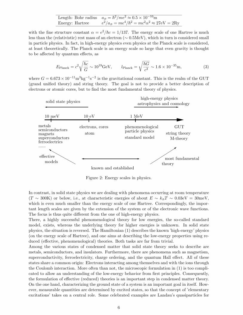
with the fine structure constant α = e2/~c = 1/137. The energy scale of one Hartree is muchless than the (relativistic) rest mass of an electron (∼ 0.5MeV), which in turn is considered smallin particle physics. In fact, in high-energy physics even physics at the Planck scale is considered,at least theoretically. The Planck scale is an energy scale so large that even gravity is thoughtto be affected by quantum effects, as

EPlanck = c2

√~cG∼ 1019GeV, lPlanck =

√~Gc3∼ 1.6× 10−35m, (3)

where G = 6.673× 10−11m3kg−1s−2 is the gravitational constant. This is the realm of the GUT(grand unified theory) and string theory. The goal is not to provide a better description ofelectrons or atomic cores, but to find the most fundamental theory of physics.

string theory

10 meV 10 eV 1 MeV

electrons, cores

atom

phenomenological

standard model

GUT

M-theory

high-energy physicsastrophysics and cosmologysolid state physics

known and established

effectivemodels theory

most fundamental

semiconductorsmagnetssuperconductorsferroelectrics......

metalsparticle physics

Figure 2: Energy scales in physics.

In contrast, in solid state physics we are dealing with phenomena occurring at room temperature(T ∼ 300K) or below, i.e., at characteristic energies of about E ∼ kBT ∼ 0.03eV = 30meV,which is even much smaller than the energy scale of one Hartree. Correspondingly, the impor-tant length scales are given by the extension of the system or of the electronic wave functions.The focus is thus quite different from the one of high-energy physics.There, a highly successful phenomenological theory for low energies, the so-called standardmodel, exists, whereas the underlying theory for higher energies is unknown. In solid statephysics, the situation is reversed. The Hamiltonian (1) describes the known ’high-energy’ physics(on the energy scale of Hartree), and one aims at describing the low-energy properties using re-duced (effective, phenomenological) theories. Both tasks are far from trivial.Among the various states of condensed matter that solid state theory seeks to describe aremetals, semiconductors, and insulators. Furthermore, there are phenomena such as magnetism,superconductivity, ferroelectricity, charge ordering, and the quantum Hall effect. All of thesestates share a common origin: Electrons interacting among themselves and with the ions throughthe Coulomb interaction. More often than not, the microscopic formulation in (1) is too compli-cated to allow an understanding of the low-energy behavior from first principles. Consequently,the formulation of effective (reduced) theories is an important step in condensed matter theory.On the one hand, characterizing the ground state of a system is an important goal in itself. How-ever, measurable quantities are determined by excited states, so that the concept of ’elementaryexcitations’ takes on a central role. Some celebrated examples are Landau’s quasiparticles for

6

Fermi liquids, the phonons connected to lattice vibrations, and magnons in ferromagnets. Theidea is to treat the ground state as an effective vacuum in the sense of second quantization,with the elementary excitations as particles on that vacuum. Depending on the system, thevacuum may be the Fermi sea or some state with a broken symmetry, like a ferromagnet, asuperconductor, or the crystal lattice itself.According to P. W. Anderson,1 the description of the properties of materials rests on two princi-ples: The principle of adiabatic continuity and the principle of spontaneously broken symmetry.By adiabatic continuity we mean that complicated systems may be replaced by simpler systemsthat have the same essential properties in the sense that the two systems may be adiabaticallydeformed into each other without changing qualitative properties. Arguably the most impres-sive example is Landau’s Fermi liquid theory mentioned above. The low-energy properties ofstrongly interacting electrons are the same as those of non-interacting fermions with renormal-ized parameters. On the other hand, phase transitions into states with qualitatively differentproperties can often be characterized by broken symmetries. In magnetically ordered states therotational symmetry and the time-reversal invariance are broken, whereas in the superconduct-ing state the global gauge symmetry is. In many cases the violation of a symmetry is a guidingprinciple which helps to simplify the theoretical description considerably. Moreover, in recentyears some systems have been recognized as having topological order which may be consideredas a further principle to characterize low-energy states of matter. A famous example for this isfound in the context of the Quantum Hall effect.The goal of these lectures is to introduce these basic concepts on which virtually all more elab-orate methods are building up. In the course of this, we will cover a wide range of frequentlyencountered ground states, starting with the theory of metals and semiconductors, proceedingwith magnets, Mott insulators, and finally superconductors.

1P.W. Anderson: Basic Notions of Condensed Matter Physics, Frontiers in Physics Lecture Notes Series,Addison-Wesley (1984).

7

Chapter 1

Electrons in the periodic crystal -band structure

One of the characteristic features of many solids is the regular arrangement of their atomsforming a crystal. Electrons moving in such a crystal are subject to a periodic potential whichoriginates from the lattice of ions and an averaged electron-electron interaction (like Hartree-Fock approximation). The spectrum of extended electronic states, i.e. delocalized eigenstates ofthe Schrodinger equation, form bands of allowed energies and gaps of ”forbidden” energies.There are two limiting starting points towards the understanding of the band formation: (1)the free electron gas whose continuous spectrum is broken up into bands under the influence ofa periodic potential (electrons undergo Bragg scattering); (2) independent atoms are broughttogether into a lattice until the outer-most electronic states overlap and lead to delocalizedstates turning a discrete set of states into continua of electronic energies - bands. In thischapter we will address the emergence of band structures from these two limiting cases. Theband structure of electrons is essential for the basic classification of materials into metals andinsulators (semiconductors).

1.1 Symmetries of crystals

1.1.1 Space groups of crystals

Most solids consist of a regular lattice of atoms with perfectly repeating structures. The minimalrepeating unit of such a lattice is the unit cell. The symmetries of a crystal are contained inthe space group R, a group of symmetry operations (translations, rotations, the inversion orcombinations) under which the crystal is left invariant. In three dimensions, there are 230different space groups1 (cf. Table 1.1).

1All symmetry transformations form together a set which has the properties of a group. A group G combinedwith a multipliation ”∗” has the following properties:

• the product of two elements of G is also in G: a, b ∈ G ⇒ a ∗ b = c ∈ G.

• multiplications are associative: a ∗ (b ∗ c) = (a ∗ b) ∗ c.• a unit element e ∈ G exists with: e ∗ a = a ∗ e = a for all a ∈ G.

• for every element a ∈ G there is an inverse a−1 ∈ G with a1 ∗ a = a ∗ a1 = e.

A group with a ∗ b = b ∗ a for all pairs of element is called Abelian group, otherwise it is non-Abelian. A subsetG′ ⊂ G is called a subgroup of G, if it is a group as well.Guides to group theory in the context of condensed matter physics can be found in the textbooks

- Mildred S. Dresselhaus, Gene Dresselhaus and Ado Jorio: Group Theory - Application to the Physics ofCondensed Matter

- Peter Y. Yu and Manuel Cardona: Fundamentals of Semiconductors, Springer.

8

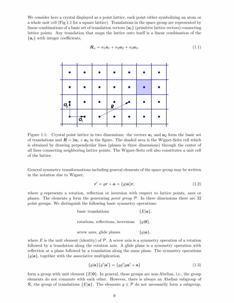
We consider here a crystal displayed as a point lattice, each point either symbolizing an atom ora whole unit cell (Fig.1.1 for a square lattice). Translations in the space group are represented bylinear combinations of a basic set of translation vectors ai (primitive lattice vectors) connectinglattice points. Any translation that maps the lattice onto itself is a linear combination of theai with integer coefficients,

Rn = n1a1 + n2a2 + n3a3. (1.1)

a2

a1

R

Figure 1.1: Crystal point lattice in two dimensions: the vectors a1 and a2 form the basic setof translations and R = 2a1 + a2 in the figure. The shaded area is the Wigner-Seitz cell whichis obtained by drawing perpendicular lines (planes in three dimensions) through the center ofall lines connecting neighboring lattice points. The Wigner-Seitz cell also constitutes a unit cellof the lattice.

General symmetry transformations including general elements of the space group may be writtenin the notation due to Wigner,

r′ = gr + a = g|ar, (1.2)

where g represents a rotation, reflection or inversion with respect to lattice points, axes orplanes. The elements g form the generating point group P. In three dimensions there are 32point groups. We distinguish the following basic symmetry operations:

basic translations E|a,

rotations, reflections, inversions g|0,

screw axes, glide planes g|a,

where E is the unit element (identity) of P. A screw axis is a symmetry operation of a rotationfollowed by a translation along the rotation axis. A glide plane is a symmetry operation withreflection at a plane followed by a translation along the same plane. The symmetry operationsg|a, together with the associative multiplication

g|ag′|a′ = gg′|ga′ + a (1.3)

form a group with unit element E|0. In general, these groups are non-Abelian, i.e., the groupelements do not commute with each other. However, there is always an Abelian subgroup ofR, the group of translations E|a. The elements g ∈ P do not necessarily form a subgroup,

9

because some of these elements (e.g., screw axes or glide planes) leave the lattice invariant onlyin combination with a translation. Nevertheless, the relation

g|aE|a′g|a−1 = E|ga′ (1.4)

g|a−1E|a′g|a = E|g−1a′ (1.5)

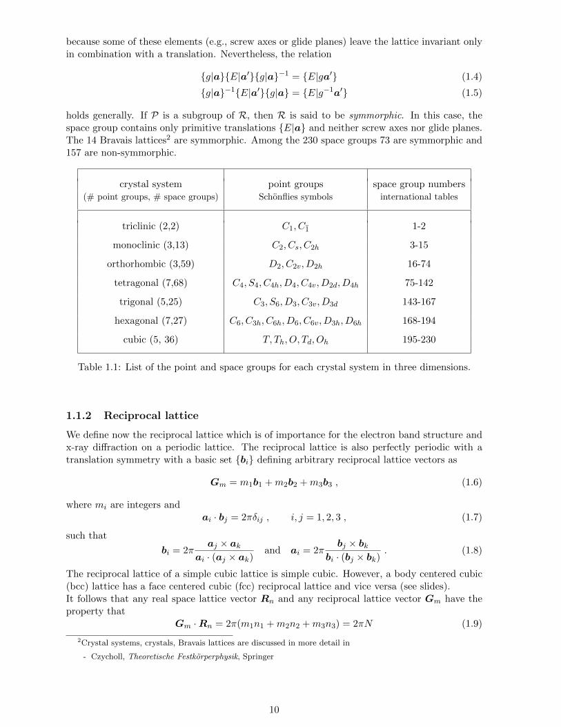
holds generally. If P is a subgroup of R, then R is said to be symmorphic. In this case, thespace group contains only primitive translations E|a and neither screw axes nor glide planes.The 14 Bravais lattices2 are symmorphic. Among the 230 space groups 73 are symmorphic and157 are non-symmorphic.

crystal system point groups space group numbers(# point groups, # space groups) Schonflies symbols international tables

triclinic (2,2) C1, C1 1-2

monoclinic (3,13) C2, Cs, C2h 3-15

orthorhombic (3,59) D2, C2v, D2h 16-74

tetragonal (7,68) C4, S4, C4h, D4, C4v, D2d, D4h 75-142

trigonal (5,25) C3, S6, D3, C3v, D3d 143-167

hexagonal (7,27) C6, C3h, C6h, D6, C6v, D3h, D6h 168-194

cubic (5, 36) T, Th, O, Td, Oh 195-230

Table 1.1: List of the point and space groups for each crystal system in three dimensions.

1.1.2 Reciprocal lattice

We define now the reciprocal lattice which is of importance for the electron band structure andx-ray diffraction on a periodic lattice. The reciprocal lattice is also perfectly periodic with atranslation symmetry with a basic set bi defining arbitrary reciprocal lattice vectors as

Gm = m1b1 +m2b2 +m3b3 , (1.6)

where mi are integers andai · bj = 2πδij , i, j = 1, 2, 3 , (1.7)

such that

bi = 2πaj × ak

ai · (aj × ak)and ai = 2π

bj × bkbi · (bj × bk)

. (1.8)

The reciprocal lattice of a simple cubic lattice is simple cubic. However, a body centered cubic(bcc) lattice has a face centered cubic (fcc) reciprocal lattice and vice versa (see slides).It follows that any real space lattice vector Rn and any reciprocal lattice vector Gm have theproperty that

Gm ·Rn = 2π(m1n1 +m2n2 +m3n3) = 2πN (1.9)

2Crystal systems, crystals, Bravais lattices are discussed in more detail in

- Czycholl, Theoretische Festkorperphysik, Springer

10

with N being an integer. This allows us to expand any function f(r) periodically in the reallattice as

f(r) =∑G

fGeiG·r (1.10)

with the obvious property: f(r +R) = f(r). The coefficients are given by

fG =1

ΩUC

∫UC

d3rf(r)e−iG·r (1.11)

where the integral runs over the unit cell of the periodic lattice with the volume ΩUC. Finally, wedefine the (first) Brillouin zone as the ”Wigner-Seitz cell” constructed in the reciprocal lattice(see Fig.1.1 and 1.2).

1.2 Bloch’s theorem and Bloch functions

We consider a Hamiltonian H of electrons invariant under a discrete set of lattice translationsE|a, a symmetry introduced by a periodic potential. This implies that the correspondingtranslation operator Ta on the Hilbert space commutes with the Hamiltonian H = He + Hie

(purely electronic Hamiltonian He, interaction between electrons and ions Hie),

[Ta,H] = 0. (1.12)

This translation operator is defined through Ta|r〉 = |r+a〉. Neglecting the interactions amongelectrons, which would be contained in He, we are left with a single particle problem

H → H0 =p2

2m+ V (r), (1.13)

where r and p are position and momentum operators, and

V (r) =∑j

Vion(r −Rj), (1.14)

describes the potential landscape of the single particle in the ionic background. With Rj beingthe position of the j-th ion, the potential V (r) is by construction periodic, with V (r+a) = V (r)for all lattice vectors a, and represents Hie. Therefore, H0 commutes with Ta. For a Hamilto-nian H0 commuting with the translation operator Ta, the eigenstates of H0 are simultaneouslyeigenstates of Ta.Bloch’s theorem states that the eigenvalues of Ta lie on the unit circle of the complex plane,which ensures that these states are extended. This means

Taψ(r) = ψ(r − a) = λaψ(r) , Tlaψ(r) = ψ(r − la) = T laψ(r) = λlaψ(r) (1.15)

with l an integer. The wave function delocalized in a periodic lattice satisfies,

|ψ(r)|2 = |ψ(r − la)|2 = |λla|2|ψ(r)|2 , (1.16)

requiring|λa| = 1 ⇒ λa = eiϕa . (1.17)

This condition is satisfied if we express the wave function as product of a plane wave eik·r anda periodic Bloch function uk(r)

ψn,k(r) =1√Ωeik·run,k(r) . (1.18)

11

with

Taun,k(r) = un,k(r − a) = un,k(r), (1.19)

Taψn,k(r) = ψn,k(r − a) = e−ik·aψn,k(r), (1.20)

H0ψn,k(r) = εn,kψn,k(r). (1.21)

The integer n is a quantum number called band index, k is the pseudo-momentum (wave vector)and Ω represents the volume of the system. Note that the eigenvalue of ψn,k(r) with respect to

Ta, e−ik·a, implies periodicity in the reciprocal space, the k-space, because ei(k+G)·a = eik·a forall reciprocal lattice vectors G. We may, therefore, restrict k to the first Brillouin zone.Bloch’s theorem simplifies the initial problem to the so-called Bloch equation for the periodicfunction uk, (

(p+ ~k)2

2m+ V (r)

)uk(r) = εkuk(r), (1.22)

where we suppress the band index to simplify the notation. This equation follows from therelation

p eik·ruk(r) = eik·r(p+ ~k)uk(r), (1.23)

which can be used for more complex forms of the Hamiltonian as well. There are variousnumerical methods which allow to compute rather efficiently the band energies εk for a givenHamiltonian H.

1.3 Nearly free electron approximation

We start here from the limit of free electrons assuming the periodic potential V (r) is weak.Using Eqs.(1.10) and (1.11) we expand the periodic potential,

V (r) =∑G

VGeiG·r, (1.24)

VG =1

ΩUC

∫UC

d3r V (r)e−iG·r. (1.25)

The potential is real and we assume it also to be invariant under inversion (V (r) = V (−r)),leading to VG = V ∗−G = V−G. Note that the uniform component V0 corresponds to an irrelevantenergy shift and may be set to zero. Because of its periodicity, the Bloch function uk(r) isexpressed in the same way,

uk(r) =∑G

cGe−iG·r, (1.26)

where the coefficients cG = cG(k) are functions of k, in general. Inserting this Ansatz and theexpansion (1.24) into the Bloch equation, (1.22), we obtain a linear eigenvalue problem for theband energies εk, (

~2

2m(k −G)2 − εk

)cG +

∑G′

VG′−G cG′ = 0. (1.27)

This represents an eigenvalue problem in infinite dimensions with eigenvectors cG(k) and eigen-values εk as band energies. These εk include corrections to the bare parabolic dispersion,

ε(0)k = ~2k2/2m, due to the potential V (r). Obviously, the dispersion ε

(0)k is naturally parabolic

12

in absence of the potential V (r) whereby the eigenstates would be simply plane waves. As alowest order approach we obtain the approximative energy spectrum within the first Brillouinzone, considering only all parabolic bands of the type εk(G) = ~2(k−G)2/2m centered aroundthe reciprocal wave vectors G (see dashed line in Fig.1.2)).

We illustrate here the nearly free electron method using the case of a one-dimensional lattice.Assuming that the periodic modulation of the potential is weak, say |VG| ~2G2/2m (taking Gas a characteristic wavevector in the periodic system), the problem (1.27) can be simplified. Letus start with the lowest energy values around the center of the first Brillouin zone, i.e. k ≈ 0(|k| π/a). For the lowest energy eigenvalue we solve Eq.(1.27) by

cG ≈

1 for G = 0

− 2mVG~2(k −G)2 − k2 1 for G 6= 0

(1.28)

leading to the energy eigenvalue

εk ≈~2k2

2m−∑G 6=0

|VG|2~2

2m [(k −G)2 − k2]≈ ~2k2

2m∗+ E0 (1.29)

with

E0 = −∑G 6=0

|λG|2~2

2mG2 (1.30)

and

1

m∗=

1

m

1− 4∑G6=0

|λG|2 (1.31)

with λG = VG/~2G2/2m (|λG| 1). We observe that εk is parabolic with a slightly modified(effective) mass, m→ m∗ > m. Note that this result resembles the lowest order corrections in theRayleigh-Schrodinger perturbation theory for a non-degenerate state. This solution correspondsto the lowest branch of the band structure within this approach (see Fig.1.2). The parabolicapproximation of the band structure at a symmetry point with an effective massm∗, is a standardway to approximate band tops or bottoms. It is called k · p-approximation (”k-dot-p”).We stay at the zone center and address the next eigenstates which are dominated by the parabolaoriginating from G± = ±2π/a = ±G which cross for k = 0 at a value ~2G2/2m. Restrictingourselves to these two components we obtain the two-dimensional eigenvalue equation system, ~2

2m(k − G)2 − εk V−2G

V2G~2

2m(k + G)2 − εk

cG

c−G

= 0 . (1.32)

The eigenvalues are obtained through the secular equation,

det

~2

2m(k − G)2 − εk V ∗

2G

V2G~2

2m(k + G)2 − εk

= 0 , (1.33)

leading to

εk± =1

2

~2

2m

(k + G)2 + (k − G)2

±√(

~2

2m

(k + G)2 − (k − G)2

)2

+ 4|V2G|2

=~2

2mG2 ± |V2G|+

~2

2m∗±k2

(1.34)

13

with the effective mass1

m∗±≈ 1

m

(1± 2|λG|−1

)(1.35)

where m∗+ > 0 and m∗− < 0 as |λG| 1. We observe a energy band gap separating two bandswith opposite curvature (see Fig.1.2). Note that the curvature diverges for V2G → 0 as m∗± → 0.The wavefunctions at k = 0 are given by

c(±)

−G = ∓V ∗

2G

|V2G|c

(±)

+G= ∓c(±)

+G(1.36)

where we have chosen V2G to be real and positive. Thus,

uk=0(x) =

sin Gx for εk=0,+

cos Gx for εk=0,−

(1.37)

one being even and the other odd under parity operation x→ −x.A similar analysis can be done at the boundary of the first Brillouin zone where two energyparabolas cross. For example at k = ±π/a we find the two dominant contributions originatefrom G = +2π/a and −2π/a, respectively, together with G = 0. Also here the energy eigenvaluesshow a band gap with parabolic bands centered at k = ±π/a (boundary of the first Brillouinzone in one-dimension) with positive and negative effective mass (see Fig.1.2). Analogous asfor the band center we can distinguish the wavefunction with even and odd parity for the twobands at the Brillouin zone boundary. Indeed every crossing energy parabola centered arounddifferent reciprocal lattice points contributes to a band gap. By construction we can extend theband structure beyond the first Brillouin zone and find a periodic energy spectrum with

εk+G = εk (1.38)

where G is a reciprocal lattice ”vector”. Moreover, we find in Fig.1.2 that ε−k = εk due to parityas well as time reversal symmetry, like for free electrons.

! 2a a

2a0! a

E

k

band gap

1st Brillouin zone

Figure 1.2: Band structure obtained by the nearly free electron approximation for a regularone-dimensional lattice.

14

1.4 Tight-binding approximation

We consider now a regular lattice of atoms which are well separated such that their atomicorbitals have small overlaps only. Therefore, in a good approximation the electronic states arerather well represented by localized atomic orbitals, φn(r). The discrete spectrum of the atomsis obtained with the atomic Hamiltonian,

Ha(R)φn(r −R) = εnφn(r −R) , (1.39)

for an atom located at position R, so that

Ha(R) =p2

2m+ Va(r −R) (1.40)

with Va(r) as the rotation symmetric atomic potential as shown in Fig.1.3 a). The index n shallinclude all necessary quantum numbers, besides the principal quantum number also angularmomentum (l,m) and spin. The single-particle Hamiltonian combines all the potentials of theatoms on the regular lattice (see Fig.1.3 b)),

H =p2

2m+∑Rj

Va(r −Rj) = Ha(Rj) + ∆VRj (r) (1.41)

where we single out one atomic potential (the choice of Rj is arbitrary) and introduce thecorrection

∆VRj (r) =∑

Rj′ 6=RjVa(r −Rj′) . (1.42)

b)a) V

localized

atomic orbitals

extended states

V

Figure 1.3: Potential landscape: a) a single atomic Coulomb potential yields a discrete spectrumelectronic states; b) atoms arranged in a regular lattice give rise to a periodic potential whichclose to the atom sites look much like the attractive Coulomb-like potential. Electron statesof low energy can be considered as practically localized at the atom sites, as the extension oftheir wave functions is very small. The higher energy states, however, extend further and candelocalize to form itinerant electron states which form bands.

1.4.1 Linear combination of atomic orbitals - LCAO

We use here a linear combination of atomic orbitals (LCAO) to approximate the extended Blochstates

ψnk(r) =1√N

∑Rj

eik·Rjφn(r −Rj) , (1.43)

15

where N denotes the number of lattice sites. This superposition has obviously the properties ofa Bloch function through ψnk(r + a) = eik·aψnk(r) for all lattice vectors a. Note that this issimilar to the Hund-Mullikan ansatz for molecular orbitals.First we determine the norm of this Bloch function,

〈1〉nn′(k) =

∫d3rψnk(r)∗ψn′k(r) =

1

N

∑Rj ,Rj′

∫d3reik·(Rj′−Rj)φ∗n(r −Rj)φn′(r −Rj′)

=∑Rj

∫d3re−ik·Rjφ∗n(r −Rj)φn′(r)

= δnn′ +∑Rj 6=0

e−ik·Rjαnn′(Rj)

(1.44)where due to translational invariance in the lattice we may set Rj′ = 0 eliminating the sum overRj′ and dropping the factor 1/N . To estimate the energy we calculate,

〈H〉nn′(k) =1

N

∑Rj ,Rj′

∫d3reik·(Rj′−Rj)φ∗n(r −Rj)Ha(Rj′) + ∆VRj′ (r)φn′(r −Rj′)

= En′〈1〉nn′(k) +1

N

∑Rj ,Rj′

∫d3reik·(Rj′−Rj)φ∗n(r −Rj)∆VRj′ (r)φn′(r −Rj′)

= En′〈1〉nn′(k) + ∆Enn′ +∑Rj 6=0

e−ik·Rjγnn′(Rj)

(1.45)where

∆Enn′ =

∫d3rφ∗n(r)∆VRj′=0(r)φn′(r) (1.46)

and

γnn′(Rj) =

∫d3rφ∗n(r −Rj)∆VRj′=0(r)φn′(r) . (1.47)

From this we can now calculate the band energies through the secular equation,

det [〈H〉nn′(k)− εk〈1〉nn′(k)] = 0. (1.48)

The merit of the approach is that the tightly bound atomic orbitals have only weak overlap suchthat both αnn′(Rj) and γnn′(Rj) fall off very quickly with growing Rj . Mostly it is sufficient totake Rj connecting nearest-neighbor and sometimes next-nearest-neighbor lattice sites. This isfor example fine for bands derived from 3d-orbitals among the transition metals such as Mn, Feor Co etc.. Also transition metal oxides are well represented in the tight-binding formulation.Alkali metals in the first row of the periodic table, Li, Na, K etc. are not suitable becausetheir outermost s-orbitals have generally a large overlap. Note that the construction of theHamiltonian matrix ensures that k → k + G does not change εk, if G is a reciprocal latticevector.

1.4.2 Band structure of s-orbitals

The most simple case of a non-degenerate atomic orbital is the s-orbital with vanishing angularmomentum (` = 0). Since these orbitals have rotation symmetric wavefunctions, φs(r) = φs(|r|),the matrix elements only depend on the distance between sites, |Rj |. As an example we considera simple cubic lattice taking nearest-neighbor (Rj = ±(a, 0, 0), ±(0, a, 0) and ±(0, 0, a)) and

16

next-nearest-neighbor coupling (Rj = (±a,±a, 0), (±a, 0,±a), (0, ±a, ±a)) into account. Forsimplicity we will neglect the overlap integrals αss(Rj), as they are not important to describethe essential feature of the band structure.

γss(Rj) =

−t Rj connects nearest neighbors

−t′ Rj connects next nearest neighbors(1.49)

which leads immediately to

εk = Es + ∆Es − tn.n.∑Rj

e−ik·Rj − t′n.n.n.∑Rj

e−ik·Rj

= Es + ∆Es − 2tcos(kxa) + cos(kya) + cos(kza)

−4t′[cos(kxa) cos(kya) + cos(kya) cos(kza) + cos(kza) cos(kxa)

(1.50)

Note that ∆VRj (r) ≤ 0 in most cases due to the attractive ionic potentials. Therefore t, t′ > 0.There is a single band resulting from this s-orbital, as shown in Fig.1.4. We may also considerthe k · p-approximation at k = 0 which yields an effective mass

εk = Es + ∆Es + 6t+ 12t′ +~2

2m∗k2 + · · · (1.51)

with1

m∗=

2

~2(t+ 4t′) . (1.52)

Note that t and t′ shrink quickly, if with growing lattice constant a the overlap of atomic orbitalsdecreases.

1.4.3 Band structure of p-orbitals

We turn to the case of degenerate orbitals. The most simple case is the p-orbital with angularmomentum l = 1 which is three-fold degenerate, represented by the atomic orbital wavefunctionsof the form,

φx(r) = xϕ(r), φy(r) = yϕ(r), φz(r) = zϕ(r) , (1.53)

with ϕ(r) being a rotation symmetric function. Note that x, y, z can be represented by spher-ical harmonics Y1,m. We assume again a simple cubic lattice such that these atomic orbitalsremain degenerate. Analyzing the properties of the integrals by symmetry, we find,

Ex = Ey = Ez = Ep and ∆Enn′ = ∆Ep δnn′ . (1.54)

The overlaps Eq.(1.47) for nearest neighbors,

γxx(Rj) =

t Rj = (±a, 0, 0) ‖ x (σ − bonding)

−t′ Rj = (0,±a, 0), (0, 0,±a) ⊥ x (π − bonding)(1.55)

and analogous for γyy and γzz, while γnn′ = 0, if n 6= n′. For next-nearest neighbors by symmetrywe obtain,

γxx(Rj) =

t Rj = (±a,±a, 0), (±a, 0,±a)

−t′ Rj = (0,±a,±a)(1.56)

17

s-orbitals

p-orbitals

Figure 1.4: Band structures derived from atomic orbitals with s- (one band, upper panel) andp-symmetry (three bands, lower panel) in a simple cubic lattice. Left side: First Brillouin zoneof the simple cubic lattice. Dispersion given along the k-line connecting Γ−X−R−Γ−M . Wechoose the parameters: t′ = 0.2t for the s-orbitals; t′ = 0.2t, t = 0.1t, t′ = 0.05t and t′′ = 0.15t.For the band derived from atomic p-orbitals, the irreducible representations of the bands aregiven at the symmetry points: Γ−15 (d = 3); X−2 (d = 1) , X−5 (d = 2); R−15 (d = 3); M−2 (d = 1),M−5 (d = 2) where d is the dimension of the representation showing the degeneracy.

and analogous for γyy and γzz. Next-nearest neighbor coupling also allows for inter-orbitalmatrix elements, e.g.

γxy(Rj) = γyx(Rj) = t′′sign(RnxRny) (1.57)

for Rj = (±a,±a, 0) and analogous for γyz(Rj) and γzx(Rj). The different configuration ofnearest- and next-nearest-neighbor coupling is shown in Fig.1.5.Now we may setup the coupling matrix,

〈H〉nn′ =

Ex(k) −4t′′ sin(kxa) sin(kya) −4t′′ sin(kxa) sin(kza)−4t′′ sin(kxa) sin(kya) Ey(k) −4t′′ sin(kya) sin(kza)−4t′′ sin(kxa) sin(kza) −4t′′ sin(kya) sin(kza) Ez(k)

(1.58)

with

Ex(k) = Ep + ∆Ep + 2t cos(kxa)− 2t′(cos(kya) + cos(kza))

+4t cos(kxa)(cos(kya) + cos(kza))− 4t′ cos(kya) cos(kza)(1.59)

and analogous for Ey(k), Ez(k). The three bands derived from the atomic p-orbitals are obtainedby solving the secular equation of the type Eq.(1.48) and shown in Fig.1.4.Also in this case we may consider a k ·p-approximation around a symmetry point in the Brillouinzone. For the Γ-point we find the expansion around k = 0:

〈H〉nn′ = EΓ +

Ak2x +B(k2

y + k2z) Ckxky Ckxkz

Ckxky Ak2y +B(k2

z + k2x) Ckykz

Ckxkz Ckykz Ak2z +B(k2

x + k2y)

(1.60)

18

! - bonding

" - bonding

no coupling

nearest neighbors next- nearest neighbors

Figure 1.5: The configurations for nearest- and next-nearest-neighbor coupling between p-orbitals on different sites. The p-orbitals are depicted by the dumb-bell structured wavefunctionwith positve (blue) and negative (red) lobes. For nearest-neighbor couplings we distinguish hereσ-bonding (full rotation symmetry around connecting axis) and π-bonding (two-fold rotationsymmetry around connecting axis). Generally the coupling is weaker for π- than for σ-bonding.No coupling for symmetry reasons are obtained between orbitals in the lower panel.

with EΓ = Ep + ∆Ep + 2t− 4t′ + 4t− 4t′, A = −a2(t+ 4t), B = a2(t′ − 2t+ 2t′) and C = −4t′′.These band energies have to be determined through the secular equations and lead to threebands with anisotropic effective masses.

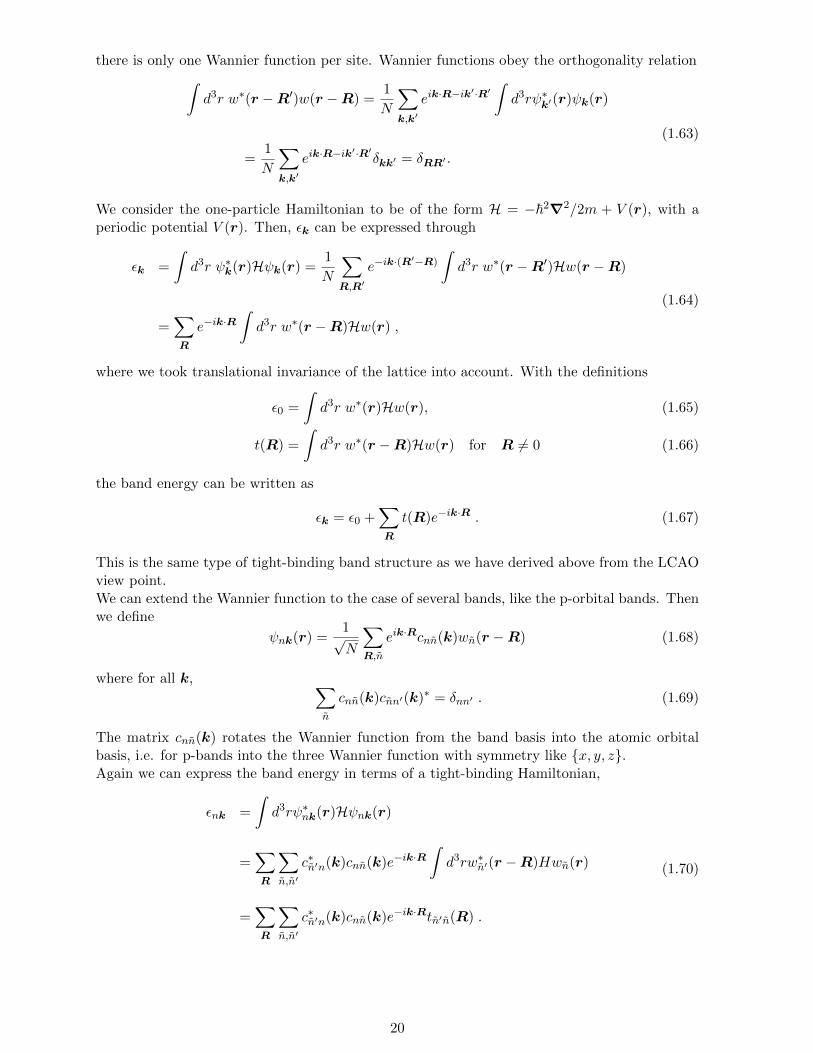
1.4.4 Wannier functions

An alternative approach to the tight-binding approximation is through Wannier functions. Theseare defined as the Fourier transformation of the Bloch wave functions,

ψk(r) =1√N

∑R

eik·Rw(r −R) w(r −R) =1√N

∑k

e−ik·Rψk(r) (1.61)

where the Wannier function w(r−R)3 is centered on the real-space lattice site R. We considerhere the situation of a non-degenerate band analogous to the atomic s-orbital case, such that

3Ambiguity of the Wannier functions: The Wannier function is not uniquely defined, because there is a ”gaugefreedom” for the Bloch function which can be multiplied by a phase factor

ψk(r)→ eiχ(k)ψk(r) (1.62)

where χ(k) is an arbitrary real function. In particular, we find different degrees of localization of w(r−R) aroundits center R depending on the choice of χ(k).

19

there is only one Wannier function per site. Wannier functions obey the orthogonality relation∫d3r w∗(r −R′)w(r −R) =

1

N

∑k,k′

eik·R−ik′·R′

∫d3rψ∗k′(r)ψk(r)

=1

N

∑k,k′

eik·R−ik′·R′δkk′ = δRR′ .

(1.63)

We consider the one-particle Hamiltonian to be of the form H = −~2∇2/2m + V (r), with aperiodic potential V (r). Then, εk can be expressed through

εk =

∫d3r ψ∗k(r)Hψk(r) =

1

N

∑R,R′

e−ik·(R′−R)

∫d3r w∗(r −R′)Hw(r −R)

=∑R

e−ik·R∫d3r w∗(r −R)Hw(r) ,

(1.64)

where we took translational invariance of the lattice into account. With the definitions

ε0 =

∫d3r w∗(r)Hw(r), (1.65)

t(R) =

∫d3r w∗(r −R)Hw(r) for R 6= 0 (1.66)

the band energy can be written as

εk = ε0 +∑R

t(R)e−ik·R . (1.67)

This is the same type of tight-binding band structure as we have derived above from the LCAOview point.We can extend the Wannier function to the case of several bands, like the p-orbital bands. Thenwe define

ψnk(r) =1√N

∑R,n

eik·Rcnn(k)wn(r −R) (1.68)

where for all k, ∑n

cnn(k)cnn′(k)∗ = δnn′ . (1.69)

The matrix cnn(k) rotates the Wannier function from the band basis into the atomic orbitalbasis, i.e. for p-bands into the three Wannier function with symmetry like x, y, z.Again we can express the band energy in terms of a tight-binding Hamiltonian,

εnk =

∫d3rψ∗nk(r)Hψnk(r)

=∑R

∑n,n′

c∗n′n(k)cnn(k)e−ik·R∫d3rw∗n′(r −R)Hwn(r)

=∑R

∑n,n′

c∗n′n(k)cnn(k)e−ik·Rtn′n(R) .

(1.70)

20

1.4.5 Tight binding model in second quantization formulation

The tight-binding formulation of band electrons can also be implemented very easily in secondquantization language and provides a rather intuitive interpretation. For simplicity we restrictourselves to the single-orbital case and define the following Fermionic operators,

c†j,s creates an electron of spin s on lattice site Rj ,

cj,s annihilates an electron of spin s on lattice site Rj ,

(1.71)

in the corresponding Wannier states. We introduce the following Hamiltonian,

H =∑j,s

ε0c†j,scj,s +

∑i,j

tij c†i,scj,s (1.72)

with tij = tji real. These coefficients tij are called ”hopping matrix elements”, since c†i,scj,sannihilates an electron on site Rj and creates one on site Ri, in this way an electron moves(hops) from Rj to Ri. Thus, this Hamiltonian represents the ”kinetic energy” of the electron.Let us now diagonalize this Hamiltonian by following Fourier transformation, equivalent to thetransformation between Bloch and Wannier functions,

c†j,s =1√N

∑k

a†kse−ik·Rj and cj,s =

1√N

∑k

akseik·Rj (1.73)

where a†ks (aks) creates (annihilates) an electron in the Bloch state with pseudo-momentum kand spin s. Inserting Eq.(1.73) into the Hamiltonian (1.72) leads to

H =∑k,k′,s

1

N

∑i

ε0ei(k−k′)·Ri +

1

N

∑i,j

tijeik·Rj−ik′·Ri

a†k′saks =

∑k,s

εk a†ksaks (1.74)

where a†ksaks = nks constitutes the number operator for electrons. The band energy is the sameas obtained above from the tight-binding approach. The Hamiltonian (1.72) will be used laterfor the Hubbard model where a real-space formulation is helpful.The real-space formulation of the kinetic energy allows also for the introduction of disorder, non-periodicity which can be most straightforwardly implemented by site dependent potentials ε0 →ε0i and to spatially (bond) dependent hopping matrix elements tij = t(Ri,Rj) 6= t(Ri −Rj).

1.5 Symmetry properties of the band structure

The symmetry properties of crystals are a helpful tool for the analysis of their band structure.They emerge from the symmetry group (space and point group) of the crystal lattice. Considerthe action Sg|a of an element g|a of the space group on a Bloch wave function ψk(r) 4

4In Dirac notation we write for the Bloch state with pseudo-momentum k as

ψk(r) = 〈r|ψk〉. (1.75)

The action of the operator Sg|a on the state |r〉 is given by

Sg|a|r〉 = |gr + a〉 and 〈r|Sg|a = 〈g−1r − g−1a|, (1.76)

such that

〈r|Sg|a|ψk〉 = ψk(g−1r − g−1a). (1.77)

The same holds for pure translations.

21

Sg|aψk(r) = ψk(g|a−1r) = ψk(g−1r − g−1a). (1.79)

Because g|a belongs to the space group of the crystal, we have [Sg|a,H0] = 0. Applying a

pure translation Ta′ = SE|a′ to this new wave function and using Eq.(1.5)

Ta′Sg|aψk(r) = Sg|aTg−1a′ψk(r) = Sg|ae−ik·(g−1a′)ψk(r)

= Sg|ae−i(gk)·a′ψk(r)

= e−i(gk)·a′Sg|aψk(r), (1.80)

the latter is found to be an eigenfunction of Ta′ with eigenvalue e−i(gk)·a′ . Remember, that,according to the Bloch theorem, we chose a basis ψk diagonalizing both Ta and H0. Thus,apart from a phase factor, the action of a symmetry transformation g|a on the wave function5

corresponds to a rotation from k to g−1k.

Sg|aψk(r) = λg|aψgk(r), (1.82)

with |λg|a|2 = 1, or

Sg|a|k〉 = λg|a|gk〉. (1.83)

in Dirac notation. Then it is easy to see that

εgk = 〈gk|H0|gk〉 = 〈k|S−1g|aH0Sg|a|k〉 = 〈k|H0|k〉 = εk. (1.84)

Consequently, there is a star-like structure of equivalent points gk with the same band energy(→ degeneracy) for each k in the Brillouin zone (cf. Fig. 1.6).For a general point k the number of equivalent points in the star equals the number of pointgroup elements for this k (without inversion). If k lies on points or lines of higher symmetry, itis left invariant under a subgroup of the point group. Consequently, the number of beams of thestar is smaller. The subgroup of the point group leaving k unchanged is called little group of k.If inversion is part of the point group, −k is always contained in the star of k. In summary, wehave the simple relations

εnk = εn,gk, εnk = εn,−k, εnk = εn,k+G. (1.85)

Note that this definition has also implications on the sequential application of transformation operators suchas

Sg1|a1Sg2|a2ψk(r) = 〈r|Sg1|a1Sg2|a2|ψk〉 = 〈g1|a1−1r|Sg2|a2|ψk〉

= 〈g2|a2−1g1|a1−1r|ψk〉 = ψk

(g2|a2−1g1|a1−1r

).

(1.78)

This is important in the context of Eq.(1.80).5Symmetry behavior of the wave function.

Sg|aψk(r) =1√ΩSg|ae

ik·r∑G

cG(k) eiG·r =1√Ωeik·(g

−1r−g−1a)∑G

cG(k) eiG·(g−1r−g−1a)

=1√Ωe−i(gk)·aei(gk)·r

∑G

cG(k) ei(gG)·r = e−i(gk)·a 1√Ωei(gk)·r

∑G

cg−1G(k) eiG·r

= e−i(gk)·a 1√Ωei(gk)·r

∑G

cG(gk) eiG·r = λg|aψgk(r),

(1.81)

where we use the fact that cG = cG(k) is a function of k with the property cg−1G(k) = cG(gk) i.e. Sg|auk(r) =ugk(r).

22

Figure 1.6: Star of k-points in the Brillouin zone with degenerate band energies: Left panel:Star of k; Right panel: contour plot of a two dimensional band εk = −2tcos(kxa)+cos(kya)+4t′ cos(kxa) cos(kya). The dots correspond to the star of k with degenerate energy values, demon-strating εnk = εn,gk.

We can also use symmetries to characterize Bloch states for given pseudo-momentum k. Let ustake a set of degenerate Bloch states belonging to the band n, |γ;n,k〉 satisfying the eigenvalueequation,

H|γ;n,k〉 = εnk|γ;n,k〉 (1.86)

For given k we consider the little group operations. Operating an element g of the little groupon a state |γ;n,k〉 we obtain again an eigenstate of the Hamiltonian H, as Sg,0 commutes withH,

Sg,0|γ, nk〉 =∑γ′

|γ′, nk〉 〈γ′, nk|Sg,0|γ, nk〉︸ ︷︷ ︸=Mγ′,γ(g)

. (1.87)

We transform only within the subspace of degenerate states |γ, nk〉 and the matrix Mγ′,γ(g) isa representation of the group element g on the vector space of eigenstates |γ, nk〉. If this rep-resentation is irreducible then its dimension corresponds to the degeneracy of the correspondingset of Bloch states.Looking back to the example of tight-binding bands derived from atomic p-orbitals (Fig.1.4).The symmetry at the Γ-point (k = 0) is the full crystal point group Oh (simple cubic lattice).The representation Γ−15 is three-dimensional corresponding to a basis set x, y, z (p-orbital).At the X-point (symmetry point on the Brillouin zone boundary) the group is reduced to D4h

(tetragonal) and the representations appearing are X−2 (one-dimensional corresponding to z)and X−5 (two-dimensional corresponding to x, y). Note that generally the little group of k haslower symmetry and leads to splitting of degeneracies as can be seen on the line Γ −M wherethe bands, degenerate at the Γ-point split up into three and combine again at the M -pointinto two level of degeneracy one and two, respectively. The symmetry group of the M -pointis D4h while for arbitrary k ‖ [110] it is C2v containing only four elements leaving k invariant:C2v ⊂ D4h ⊂ Oh.

1.6 Band-filling and materials properties

Due to the fermionic character of electrons each of the band states |n,k, s〉 can be occupiedwith one electron taking also the spin quantum number into account with spin s =↑ and ↓(Pauli exclusion principle). The count of electrons has profound implications on the properties

23

of materials. Here we would like to look at the most simple classification of materials based onindependent electrons.

1.6.1 Electron count and band filling

We consider here a most simple band structure in the one-dimensional tight-binding model withnearest-neighbor coupling. The lattice has N sites (N even) and we assume periodic boundaryconditions. The Hamiltonian is given by

H = −tN∑j=1

∑s=↑,↓c†j+1,scj,s + c†j,scj+1,s (1.88)

where we impose the equivalence j +N = j (periodic boundary conditions). This Hamiltoniancan be diagonalized by the Fourier transform

cj,s =1√N

∑k

ak,seiRjk (1.89)

leading to

H =∑k,s

εka†k,sak,s with εk = −2t cos ka . (1.90)

Now we request

eiRjk = ei(Rj+L)k ⇒ Lk = Nak = 2πn ⇒ k =2π

Ln =

2π

a

n

N(1.91)

with the pseudo-momentum k within the first Brillouin zone (−πa < k < π

a ) and n being aninteger. On the real-space lattice an electron can take 2N different states. Thus, for k we findthat n should take the values, n+N/2 = 1, 2, . . . , N −1, N . Note that k = −π/a and k = +π/adiffer by a reciprocal lattice vector G = 2π/a and are therefore identical. This provides thesame number of states (2N), since per k we have two spins (see Fig.1.7).We can fill these states with electrons following the Pauli exclusion principle. In Fig.1.7 we showthe two typical situations: (1) N electrons corresponding to half of the possible electrons whichcan be accommodated leading to a half-filled band and (2) 2N electrons exhausting all possiblestates representing a completely filled band. In the case of half-filling we define the Fermi energyas the energy εF of the highest occupied state, here εF = 0. This corresponds to the chemicalpotential, the energy necessary to add an electron to the system at T = 0K.An important difference between (1) and (2) is that the former allows for many different stateswhich may be separated from each other by a very small energy. For example, consideringthe ground state (as in Fig.1.7) and the excited states obtained by moving one electron fromk = π/2a (n = N/4) to k′ = 2π(1 +N/4)/Na (n = 1 +N/4), we find the energy difference

∆E = εk′ − εk ≈ 2t2π

N∝ 1

N(1.92)

which shrinks to zero for N → ∞. On the other hand, for case (2) there is only one electronconfiguration possible and no excitations within the one-band picture.

1.6.2 Metals, semiconductors and insulators

The two situations depicted in Fig.1.7 are typical as each atom (site) in a lattice contributes aninteger number of electrons to the system. So we distinguish the case that there is an odd oran even number of electrons per unit cell. Note that the unit cell may contain more than oneatom, unlike the situation shown in our tight-binding example.

24

half filled band

completely filled band

-3 -2 -1 0 1 2 3 4 n

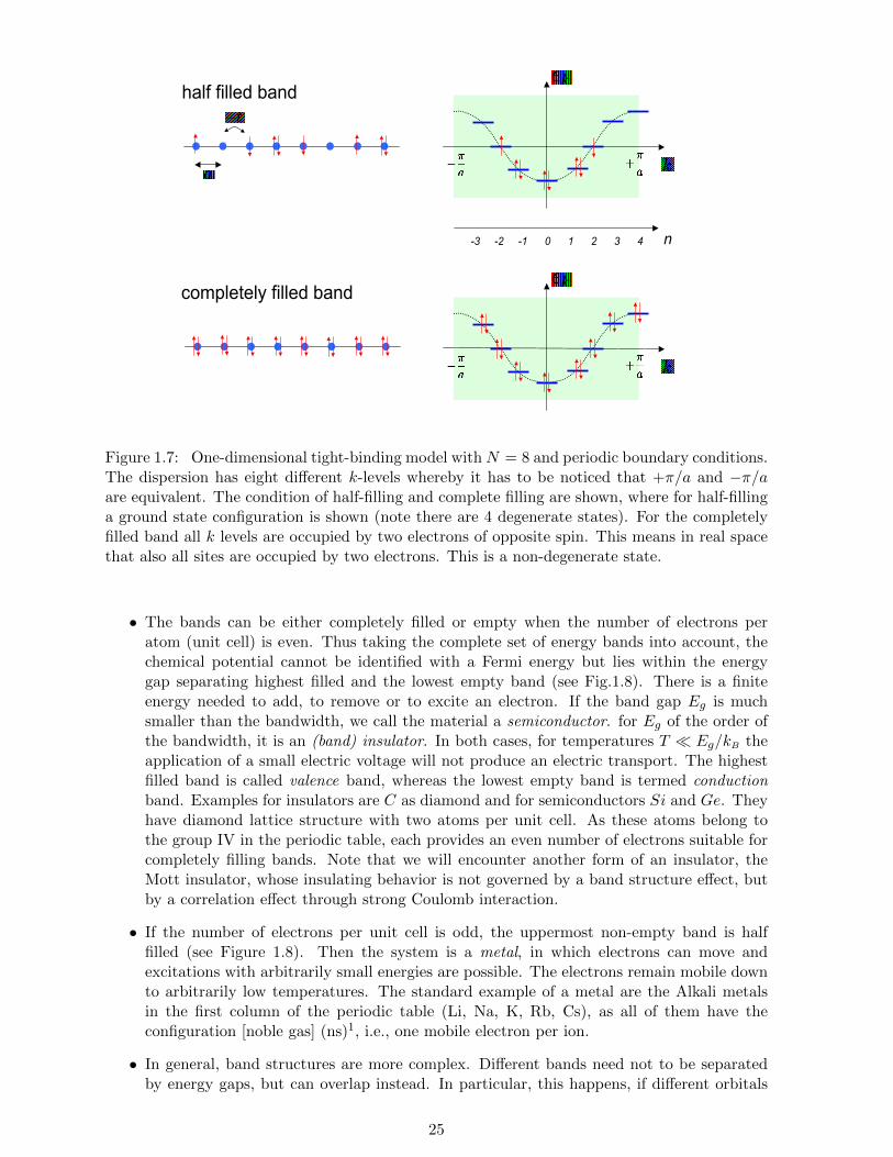
Figure 1.7: One-dimensional tight-binding model withN = 8 and periodic boundary conditions.The dispersion has eight different k-levels whereby it has to be noticed that +π/a and −π/aare equivalent. The condition of half-filling and complete filling are shown, where for half-fillinga ground state configuration is shown (note there are 4 degenerate states). For the completelyfilled band all k levels are occupied by two electrons of opposite spin. This means in real spacethat also all sites are occupied by two electrons. This is a non-degenerate state.

• The bands can be either completely filled or empty when the number of electrons peratom (unit cell) is even. Thus taking the complete set of energy bands into account, thechemical potential cannot be identified with a Fermi energy but lies within the energygap separating highest filled and the lowest empty band (see Fig.1.8). There is a finiteenergy needed to add, to remove or to excite an electron. If the band gap Eg is muchsmaller than the bandwidth, we call the material a semiconductor. for Eg of the order ofthe bandwidth, it is an (band) insulator. In both cases, for temperatures T Eg/kB theapplication of a small electric voltage will not produce an electric transport. The highestfilled band is called valence band, whereas the lowest empty band is termed conductionband. Examples for insulators are C as diamond and for semiconductors Si and Ge. Theyhave diamond lattice structure with two atoms per unit cell. As these atoms belong tothe group IV in the periodic table, each provides an even number of electrons suitable forcompletely filling bands. Note that we will encounter another form of an insulator, theMott insulator, whose insulating behavior is not governed by a band structure effect, butby a correlation effect through strong Coulomb interaction.

• If the number of electrons per unit cell is odd, the uppermost non-empty band is halffilled (see Figure 1.8). Then the system is a metal, in which electrons can move andexcitations with arbitrarily small energies are possible. The electrons remain mobile downto arbitrarily low temperatures. The standard example of a metal are the Alkali metalsin the first column of the periodic table (Li, Na, K, Rb, Cs), as all of them have theconfiguration [noble gas] (ns)1, i.e., one mobile electron per ion.

• In general, band structures are more complex. Different bands need not to be separatedby energy gaps, but can overlap instead. In particular, this happens, if different orbitals

25

semiconductor

insulator

EF

EF

EF

E EE

k kk

filled filled filled

metal semimetal

metal

Figure 1.8: Material classes according to band filling: left panel: insulator or semiconductor(partially filled bands with the Fermi level in band gap); center panel: metal (Fermi level insideband); right panel: metal or semimetal (Fermi level inside two overlapping bands).

are involved in the structure of the bands. In these systems, bands can have any fractionalfilling (not just filled or half-filled). The earth alkaline metals are an example for this(second column of the periodic table, Be, Mg, Ca, Sr, Ba), which are metallic despitehaving two (n, s)-electrons per unit cell. Systems, where two bands overlap at the Fermienergy but the overlap is small, are termed semi-metals. The extreme case, where valenceand conduction band touch in isolated points so that there are no electrons at the Fermienergy and still the band gap is zero, is realized in graphene.

The electronic structure is also responsible for the cohesive forces necessary for the formationof a regular crystal. We may also classify materials according to relevant forces. We distinguishfour major types of crystals:

Molecular crystals are formed from atoms or molecules with closed-shell atomic structuressuch as the noble gases He, Ne etc. which become solid under pressure. Here the van derWaals forces generate the binding interactions.

Ionic crystals combine different atoms, A and B, where A has a small ionization energy whileB has a large electron affinity. Thus, electrons are transferred from A to B giving apositively charged A+ and a negatively charge B−. In a regular (alternating) lattice theenergy gained through Coulomb interaction can overcome the energy expense for the chargetransfer stabilizing the crystal. A famous example is NaCl where one electron leaves Na([Ne] 3s) and is added to Cl ([Ne] 3s23p5) as to bring both atoms to closed-shell electronicconfiguration.

Covalent-bonded crystals form through chemical binding, like in the case of the H2, whereneighboring atoms share electrons through the large overlap of the electron orbital wave-function. Insulators like diamond C or semiconductors like Si or GaAs are importantexamples of this type as we will discuss later. Note that electrons of covalent bonds arelocalized between the atoms.

Metallic bonding is based on delocalized electrons (in contrast to the covalent bonds) strippedfrom their atoms. The stability of simple metals like the alkaly metals Li, Na, K etc willbe discussed later. Note that many metals, such as the noble metals Au or Pt, can also

26

involve aspects of covalent or molecular bonding through overlapping but more localizedelectronic orbitals.

1.7 Dynamics of band electrons - semiclassical approach

In quantum mechanics, the Ehrenfest theorem shows that the expectation values of the positionand momentum operators obey equations similar to the equation of motion in Newtonian me-chanics. An analogous formulation holds for electrons in a periodic potential, where we assumethat the electron may be described as a wave packet of the form

ψk(r, t) =∑k′

gk(k′)eik′·r−iεk′ t, (1.93)

where gk(k′) is centered around k in reciprocal space and has a width of ∆k. ∆k should bemuch smaller than the size of the Brillouin zone for this Ansatz to make sense, i.e., ∆k 2π/a.Therefore, the wave packet is spread over many unit cells of the lattice since Heisenberg’suncertainty principle (∆k)(∆x) > 1 implies ∆x a/2π. In this way, the pseudo-momentum kof the wave packet remains well defined. Furthermore, the applied electric and magnetic fieldshave to be small enough not to induce transitions between different bands. The latter conditionis not very restrictive in practice.

1.7.1 Semi-classical equations of motion

We introduce the rules of the semi-classical motion of electrons with applied electric and magneticfields without proof:

• The band index of an electron is conserved, i.e., there are no transitions between the bands.

• The equations of motion read6

r = vn(k) =∂εnk∂~k

, (1.96)

~k = −eE(r, t)− e

cvn(k)×H(r, t). (1.97)

• All electronic states have a wave vector that lies in the first Brillouin zone, as k and k+Glabel the same state for all reciprocal lattice vectors G.

• In thermal equilibrium, the electron density per spin in the n-th band in the volumeelement d3k/(2π)3 around k is given by

nF [εn(k)] =1

e[εn(k)−µ]/kBT + 1. (1.98)

Each state of given k and spin can be occupied only once (Pauli principle).

6A plausibility argument concerning the conservation of energy leading to the equation (1.97) is given here.The time derivative of the energy (kinetic and potential)

E = εn(k(t))− eφ(r(t)) (1.94)

has to vanish, i.e.,

0 =dE

dt=∂εn(k)

∂k· k − e∇φ · r = vn(k) ·

(~k − e∇φ

). (1.95)

From this, equation (1.97) follows directly for the electric field E = −∇φ and the Lorentz force is allowed becausethe force is always perpendicular to the velocity vn.

27

Note that ~k is not the momentum of the electron, but the so-called lattice momentum or pseudomomentum in the Bloch theory of bands. It is connected with the eigenvalue of the translationoperator on the state. Consequently, the right-hand side of the equation (1.97) is not the forcethat acts on the electron, as the forces exerted by the periodic lattice potential is not included.The latter effect is contained implicitly through the form of the band energy ε(k), which governsthe first equation.

1.7.2 Bloch oscillations

The fact that the band energy is a periodic function of k leads to a strange oscillatory behavior ofthe electron motion in a static electric field. For illustration, consider a one-dimensional systemwhere the band energy εk = −2 cos ka leads to the solution of the semi-classical equations(1.96,1.97)

~k = −eE (1.99)

⇒ k = −eEt~

(1.100)

⇒ x = −2a

~sin

(eEat

~

), (1.101)

in the presence of a homogenous electric field E. It follows immediately, that the position x ofthe electron oscillates like

x(t) =2

eEcos

(eEat

~

). (1.102)

This behavior is called Bloch oscillation and means that the electron oscillates around its initialposition rather than moving in one direction when subjected to a static electric field. This effectcan only be observed under very special conditions where the probe is absolutely clean. Theeffect is easily destroyed by damping or scattering.

time

Figure 1.9: Experimental observation of Bloch oscillation for accelerated cesium atoms trappedin an periodic optical lattice generated by standing waves of laser light: mean velocity 〈v〉 versustime [M.B. Dahan et al, Phys. Rev. Lett. 76, 4508 (1996)].

1.7.3 Current densities

We will see in chapter 6 that homogenous steady current carrying states of electron systems canbe described by the momentum distribution n(k). Assuming this property, the current density

28

follows from

j = −2e

∫BZ

d3k

(2π)3v(k)n(k) = −2e

∫BZ

d3k

(2π)3n(k)

∂ε(k)

∂~k, (1.103)

where the integral extends over all k in the Brillouin zone (BZ) and the factor 2 originatesfrom the two possible spin states of the electrons. Note that for a finite current density j, themomentum distribution n(k) has to deviate from the equilibrium Fermi-Dirac distribution inequation (1.98). It is straight forward to show that the current density vanishes for an emptyband. The same holds true for a completely filled band (n(k) = 1) where equation (1.96) implies

j = −2e

∫BZ

d3k

(2π)3

1

~∂ε(k)

∂k= 0 (1.104)

because ε(k) is periodic in the Brillouin zone, i.e., ε(k+G) = ε(k) when G is a reciprocal latticevector. Thus, neither empty nor completely filled bands can carry currents.An interesting aspect of band theory is the picture of holes. We compute the current densityfor a partially filled band in the framework of the semi-classical approximation,

j = −e∫

BZ

d3k

4π3n(k)vn(k) (1.105)

= −e[ ∫

BZ

d3k

4π3v(k)−

∫BZ

d3k

4π3[1− n(k)]v(k)

](1.106)

= +e

∫BZ

d3k

4π3[1− n(k)]v(k). (1.107)

This suggests that the current density comes either from electrons in filled states with charge−e or from ’holes’, missing electrons carrying positive charge and sitting in the unoccupiedelectronic states. In band theory, both descriptions are equivalent. However, it is usually easierto work with holes, if a band is almost filled, and with electrons if the filling of an energy bandis small.

Appendix: Approximative band structure calcuations

While the approximation of nearly free electrons gives a qualitative picture of the band structure,it rests on the assumption that the periodic potential is weak, and, thus, may be treated asa small perturbation. Only few states connected with different reciprocal lattice vectors aresufficient within this approximation. However, in reality the ionic potential is strong comparedto the electrons’ kinetic energy. This leads to strong modulations of the wave function aroundthe ions, which is not well described by slightly perturbed plane waves.

Pseudo-potential

In order to overcome this weakness of the plane wave solution, we would have to superpose avery large number of plane waves, which is not an easy task to put into practice. Alternatively,we can divide the electronic states into the ones corresponding to filled low-lying energy states,which are concentrated around the ionic core (core states), and into extended (and more weaklymodulated) states, which form the valence and conduction bands. The core electron statesmay be approximated by atomic orbitals of isolated atoms. For a metal such as aluminum (Al:1s22s22p63s23p) the core electrons correspond to the 1s-, 2s-, and 2p-orbitals, whereas the 3s-and 3p-orbitals contribute dominantly to the extended states of the valence- and conduction

29

Al1s2 2s2 2p63s23p

localized core states

1s2 2s2 2p6

extended conduction/valence states

3s23p

Figure 1.10: Separation into extended and core electronic states (example Aluminium).

bands. We will focus on the latter, as they determine the low-energy physics of the electrons.The core electrons are deeply bound and can be considered inert.We introduce the core electron states as |φj〉, with H|φj〉 = Ej |φj〉 where H is the Hamiltonianof the single atom. The remaining states have to be orthogonal to these core states, so that wemake the Ansatz

|φn,k〉 = |χnk〉 −∑j

|φj〉〈φj |χn,k〉, (1.108)

with |χn,k〉 an orthonormal set of states. Then, 〈φn,k|φj〉 = 0 holds for all j. If we choose planewaves for the |χnk〉, the resulting |φn,k〉 are so-called orthogonalized plane waves (OPW). TheBloch functions are superpositions of these OPW,

|ψn,k〉 =∑G

bk+G|φn,k+G〉, (1.109)

where the coefficients bk+G converge rapidly, such that, hopefully, only a small number of OPWsis needed for a good description.First, we again consider an arbitrary |χnk〉 and insert it into the eigenvalue equation H|φnk〉 =Enk|φnk〉,

H|χnk〉 −∑j

H|φj〉〈φj |χn,k〉 = Enk

(|χnk〉 −

∑j

|φj〉〈φj |χn,k〉)

(1.110)

or

H|χnk〉+∑j

(Enk − Ej) |φj〉〈φj |χn,k〉 = Enk|χnk〉. (1.111)

We introduce the integral operator in real space V ′ =∑

j(Enk − Ej)|φj〉〈φj |, describing a non-local and energy-dependent potential. With this operator we can rewrite the eigenvalue equationin the form

(H+ V ′)|χn,k〉 = (H0 + V + V ′)|χn,k〉 = (H+ Vps)|χn,k〉 = Enk|χnk〉. (1.112)

This is an eigenvalue equation for the so-called pseudo-wave function (or pseudo-state) |χnk〉,instead of the Bloch state |ψnk〉, where the modified potential Vps = V + V ′ is called pseudo-

potential. The attractive core potential V = V (r) is always negative. On the other hand,

30

Enk > Ej , such that V ′ is positive. It follows that Vps is weaker than both V and V ′. Anarbitrary number of core states

∑j aj |ψj〉 may be added to |χnk〉 without violating the orthog-

onality condition (1.108). Consequently, neither the pseudo-potential nor the pseudo-states areuniquely determined and may be optimized variationally with respect to the set aj in orderto optimally reduce the spatial modulation of either the pseudo-potential or the wave-function.

wave function

potenial

plane-wave approximation

pseudo-potenial

Figure 1.11: Illustration of the pseudo-potential.

rRc

Figure 1.12: Pseudopotential: Ashcroft, Heine and Abarenkov form.

If we are only interested in states inside a small energy window, the energy dependence of thepseudo-potential can be neglected, and Vps may be approximated by a standard potential (seeFigure 1.11). Such a simple Ansatz is exemplified by the atomic pseudo-potential, proposed byAshcroft, Heine and Abarenkov (AHA). The potential of a single ion is assumed to be of theform

vps(r) =

V0 r < Rc,

−Zione2

r r > Rc,(1.113)

where Zion is the charge of the ionic core and Rc its effective radius (determined by the coreelectrons). The constants Rc and V0 are chosen such that the energy levels of the outermostelectrons are reproduced correctly for the single-atom calculations. For example, the 1s-, 2s-,and 2p-electrons of Na form the ionic core. Rc and V0 are adjusted such that the one-particleproblem p2/2m+ vps(r) leads to the correct ionization energy of the 3s-electron. More flexibleapproaches allow for the incorporation of more experimental input into the pseudo-potential.

31

The full pseudo-potential of the lattice can be constructed from the contribution of the individualatoms,

Vps(r) =∑n

vps(|r −Rj |), (1.114)

where Rj is the lattice vector. For the method of nearly free electrons we need the Fouriertransform of the potential evaluated at the reciprocal lattice vectors,

Vps,G =1

Ω

∫d3r Vps(r)e−iG·r =

N

Ω

∫d3r vps(r)e−iG·r. (1.115)

For the AHA form (1.113), this is given by

Vps,G = −4πZione2

G2

(cos(GRc)

+V0

Zione2G

((R2

cG2 − 2) cos(GRc) + 2− 2RcG sin(GRc)

)). (1.116)

For small reciprocal lattice vectors, the zeroes of the trigonometric functions on the right-handside of (1.116) reduce the strength of the potential. For large G, the pseudo-potential decays∝ 1/G2. It is thus clear that the pseudo-potential is always weaker than the original potential.Extending this theory for complex unit cells containing more than one atom, the pseudo-potentialmay be written as

Vps(r) =∑n,α

vαps(|r − (Rj +Rα)|), (1.117)

where Rα denotes the position of the α-th base atom in the unit cell. Here, vαps is the pseudo-potential of the α-th ion. In reciprocal space,

Vps,G =N

Ω

∑α

e−iG·Rα∫d3r vαps(|r|)e−iG·r (1.118)

=∑α

e−iG·RαFα,G. (1.119)

The form factor Fα,G contains the information of the base atoms and may be calculated orobtained by fitting experimental data.

Augmented plane wave

We now consider a method introduced by Slater in 1937. It is an extension of the so-calledWigner-Seitz cell method (1933) and consists of approximating the crystal potential by a so-called muffin-tin potential. The latter is a periodic potential, which is taken to be sphericallysymmetric and position dependent around each atom up to a distance rs, and constant for largerdistances. The spheres of radius rs are taken to be non-overlapping and are contained completelyin the Wigner-Seitz cell7 (Figure 1.13).The advantage of this decomposition is that the problem can be solved using a divide-and-conquer strategy. Inside the muffin-tin radius we solve the spherically symmetric problem, whilethe solutions on the outside are given by plane waves; the remaining task is to match the

7The Wigner-Seitz cell is the analogue of the Brillouin zone in real space. One draws planes cutting eachline joining two atoms in the middle, and orthogonal to them. The smallest cell bounded by these planes is theWigner-Seitz cell.

32

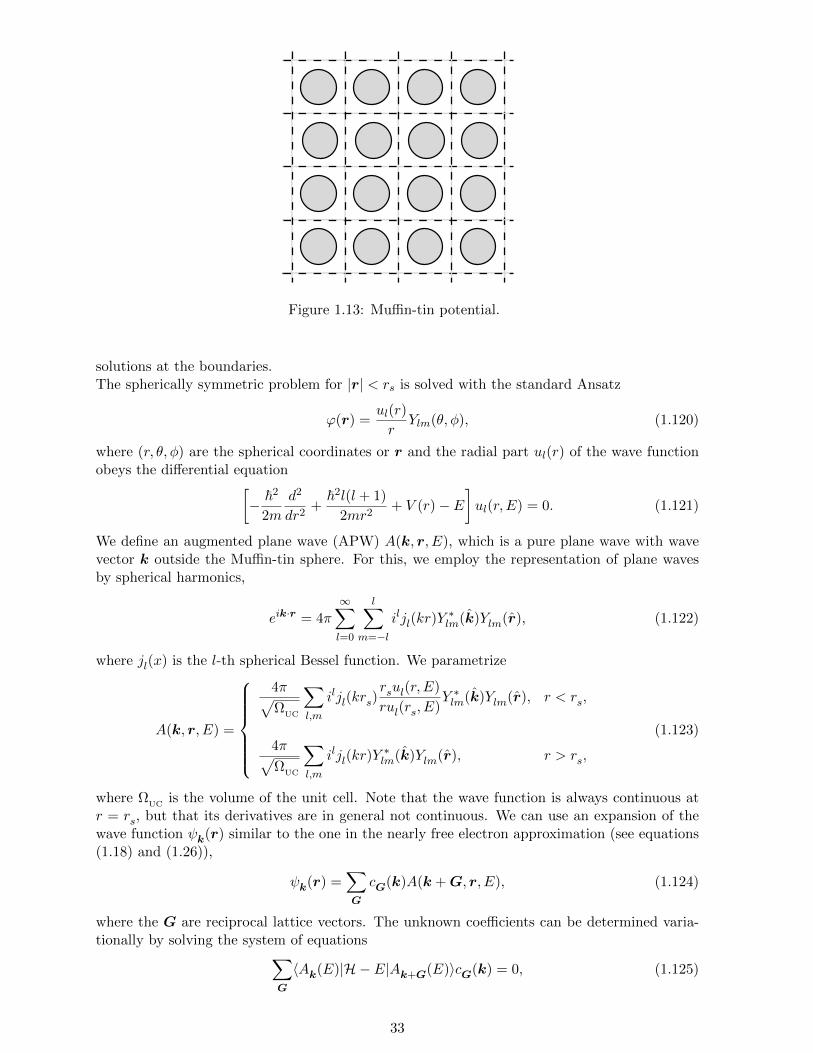
Figure 1.13: Muffin-tin potential.

solutions at the boundaries.The spherically symmetric problem for |r| < rs is solved with the standard Ansatz

ϕ(r) =ul(r)

rYlm(θ, φ), (1.120)

where (r, θ, φ) are the spherical coordinates or r and the radial part ul(r) of the wave functionobeys the differential equation[

− ~2

2m

d2

dr2+

~2l(l + 1)

2mr2+ V (r)− E

]ul(r, E) = 0. (1.121)

We define an augmented plane wave (APW) A(k, r, E), which is a pure plane wave with wavevector k outside the Muffin-tin sphere. For this, we employ the representation of plane wavesby spherical harmonics,

eik·r = 4π

∞∑l=0

l∑m=−l

iljl(kr)Y∗lm(k)Ylm(r), (1.122)

where jl(x) is the l-th spherical Bessel function. We parametrize

A(k, r, E) =

4π√Ω

UC

∑l,m

iljl(krs)rsul(r, E)

rul(rs, E)Y ∗lm(k)Ylm(r), r < rs,

4π√Ω

UC

∑l,m

iljl(kr)Y∗lm(k)Ylm(r), r > rs,

(1.123)

where ΩUC

is the volume of the unit cell. Note that the wave function is always continuous atr = rs, but that its derivatives are in general not continuous. We can use an expansion of thewave function ψk(r) similar to the one in the nearly free electron approximation (see equations(1.18) and (1.26)),

ψk(r) =∑G

cG(k)A(k +G, r, E), (1.124)

where the G are reciprocal lattice vectors. The unknown coefficients can be determined varia-tionally by solving the system of equations∑

G

〈Ak(E)|H − E|Ak+G(E)〉cG(k) = 0, (1.125)

33

where

〈Ak(E)|H − E|Ak′(E)〉 =

(~2k · k′

2m− E

)Ω

UCδk,k′ + Vk,k′ (1.126)

with

Vk,k′ = 4πr2s

[−(~2k · k′

2m− E

)j1(|k − k′|rs)|k − k′|

+∞∑l=0

~2

2m(2l + 1)Pl(k · k

′)jl(krs)jl(k

′rs)u′l(rs, E)

ul(rs, E)

]. (1.127)

Here, Pl(z) is the l-th Legendre polynomial and u′ = du/dr. The solution of (1.125) yieldsthe energy bands. The most difficult parts are the approximation of the crystal potential bythe muffin-tin potential and the computation of the matrix elements in (1.125). The rapidconvergence of the method is its big advantage: just a few dozens of G-vectors are needed andthe largest angular momentum needed is about l = 5. Another positive aspect is the fact thatthe APW-method allows the interpolation between the two extremes of extended, weakly boundelectronic states and tightly bound states.

34

Chapter 2

Semiconductors

The technological relevance of semiconductors can hardly be overstated. In this chapter, wereview some of their basic properties. Regarding the electric conductivity, semiconductors areplaced in between metals and insulators. Normal metals are good conductors at all temperatures,and the conductivity usually increases with decreasing temperature. On the other hand, forsemiconductors and insulators the conductivity decreases upon cooling (see Figure 2.1).

σ

0 0TT

semiconductor/isolator metal

σ

Figure 2.1: Schematic temperature dependence of the electric conductivity for semiconductorsand metals.

We will see that the conductivity may be written as

σ =ne2τ

m, (2.1)

where n is the density of mobile electrons, τ is the average time between two scattering eventsof the electrons, and m and e are the electronic mass and charge, respectively. In metals, n isindependent of temperature, whereas the scattering time τ decreases with increasing tempera-ture. Thus, τ determines majorly the temperature dependence of the conductivity in metals.On the other hand, insulators and semiconductors have no mobile charges at T = 0. At finitetemperature, charges are induced by thermal excitations which have to overcome the band gap1

Eg between the valence and the conduction band, yielding

n ∼ n0

(T

T0

)3/2

e−Eg/2kBT , (2.3)

1Actually, one has to count both the excited electrons in the conduction band and the resulting holes in thevalence band, as both contribute to the current,

j = (σ+ + σ−)E, with σ± =n±e

2τ±m±

, (2.2)

where + and − stand for holes and electrons, respectively, and n+ = n− holds for thermal excitation. Note that,in general, the effective masses and scattering times are not the same for the valence and conduction bands.

35

where T0 = 300K and the electron density in the material n0 is typically 1020 cm−3. Forinsulators, the energy gap is huge, e.g., 5.5 eV for diamond. Consequently, the charge carrierdensity at room temperature T = 300K is around n ∼ 10−27cm−3. For a higher charge carrierdensity n ∼ 103 − 1011cm−3, smaller gaps Eg ∼ 0.5 − 1eV are necessary. Materials witha band gap in this regime are not fully isolating and therefore are termed semiconductors.However, the carrier densities of both insulators and semiconductors are dwarfed by the electrondensity in metals contributing to current transport (nmetal ∼ 1023 − 1024cm−3). Adding asmall amount of impurities in semiconductors, a process called doping with acceptors or donors,their conductivity can be engineered in various ways, rendering them useful as components ininnumerable applications.

2.1 The band structure of the elements in group IV

2.1.1 Crystal and band structure

The most important semiconductor for technological applications is silicon (Si) that – like carbon(C), germanium (Ge) and tin (Sn) – belongs to the group IV of the periodic table. Theseelements have four electrons in their outermost shell in the configuration (ns)2(np)2 (n=2 forC, n=3 for Si, n=4 for Ge, and n=5 for Sn). All four elements form crystals with a diamondstructure (cf. Figure 2.2), i.e., a face-centered cubic lattice with a unit cell containing two atomslocated at (0, 0, 0) and (1

4 ,14 ,

14) (for Sn this is called α-Sn). The crystal structure is stabilized

by hybridization of the four valence electrons, leading to covalent bonding of oriented orbitals,

|ψ1〉 = |ns〉+ |npx〉+ |npy〉+ |npz〉, |ψ2〉 = |ns〉+ |npx〉 − |npy〉 − |npz〉,|ψ3〉 = |ns〉 − |npx〉+ |npy〉 − |npz〉, |ψ4〉 = |ns〉 − |npx〉 − |npy〉+ |npz〉. (2.4)

Locally, the nearest neighbors of each atom form a tetrahedron around it, which leads to thediamond structure of the lattice.

Figure 2.2: The crystal structure of diamond corresponds to two face-centered cubic laticesshifted by a quarter of lattice spacing along the (1,1,1) direction.

The band structure of these materials can be found around the Γ-point by applying the free-electron approximation discussed in the previous chapter. Γ1 is the corresponding representationto the parabolic band centered around the center of the Brillouin zone (0, 0, 0). Note that thereciprocal lattice of a face-centered cubic (fcc) lattice is body-centered cubic (bcc). The Brillouinzone of a fcc crystal is embedded in a bcc lattice as illustrated in Figure 2.3).The next multiplet with an energy of ε = 6π2~2/ma2 derives from the parabolic bands emanatingfrom the neighboring Brillouin zones, with G = G(±1,±1,±1) and G = 2π/a. The eight states

36

X

kx

ky

kz

LΛ

K

ΣΓ

∆

Figure 2.3: The Brillouin zone of a face-centered cubic crystal (in real space) is embedded in abcc lattice.

are split into Γ1⊕Γ2⊕Γ15⊕Γ25. The magnitude of the resulting energies are obtained from bandstructure calculations, lifting the energy degeneracy εΓ25

< εΓ15< εΓ2

< εΓ1in the presence of a

periodic potential V (r). The essential behavior of the low-energy band structure of C and Si isshown in Figure 2.4.

C Si

L X!" #

L X!" #

Figure 2.4: Band structure of C and Si.

With two atoms per unit cell and four valence electrons, there are totally eight electrons per unitcell. It follows that the bands belonging to Γ1 (non-degenerate) and Γ25 (threefold degenerate)are completely filled. The maximum of the valence band is located at the Γ-point and belongsto the representation Γ25. Because of the existence of an energy gap between valence andconduction band, the system is not conducting at T = 0. The gap is indirect, meaning that theminimum of the conduction band and the maximum of the valence band lie at different pointsin the Brillouin zone, i.e., the gap is minimal between the Γ-point of the valence band and somefinite momentum ~k0 along the [100]-direction of the conduction band.2 A typical example of a

2Energy gaps in semiconductors and insulators are said to be direct if the wave-vector connecting the maximumof the valence band and the minimum of the conduction band vanishes. Otherwise a gap is called indirect (seeFigure 2.5).

37

semiconductor with a direct gap is GaAs, composed of one element of the third and fifth group,respectively.

indirect energy gap

k

E

k

E

∆ ∆

direct energy gap

Figure 2.5: Illustration of direct and indirect band gaps.

Next we list some facts about these materials of the group IV:

• Carbon has an energy gap of around 5.5eV in the diamond structure. Thus, in thisconfiguration it is not a semiconductor but an insulator. The large energy gap causes thetransparency of diamond in the visible range (1.5-3.5eV), as the electromagnetic energy inthis range cannot be absorbed by the electrons.

• The energy gap of silicon is 1.12eV and thus much smaller; furthermore, it is indirect.

• Germanium has an indirect gap of 0.67eV.

• GaAs has a direct energy gap of 1.43eV .

2.2 Elementary excitations in semiconductors

We consider a simple two-band model to illustrate the most basic properties of the excitationspectrum of a semiconductor. The Hamiltonian is given by

H =∑k,s

εV,kc†V,k,scV,k,s +

∑k,s

εC,kc†C,k,scC,k,s, (2.5)

where εV,k and εC,k are the band energies of the valence band and conduction band, respectively.

The operator c†nks (cnks) creates (annihilates) an electron with (pseudo-)momentum k and spins in the band n, n ∈ V,C. In the ground state |Φ0〉,

|Φ0〉 =∏k,s

c†V,k,s|0〉, (2.6)

the valence band is completely filled, whereas the conduction band is empty. The product on theright-hand side runs over all wave vectors in the first Brillouin zone. The ground state energyis given by

E0 = 2∑k

εV,k. (2.7)

38

The total momentum and spin of the ground state vanish. We next consider single electronexcitations from that ground state.3

2.2.1 Electron-hole excitations

A simple excitation of the system consists of removing an electron (i.e., creating a hole) fromthe valence band and inserting it into the conduction band. We write such an excitation as

|k + q, s;k, s′〉 = c†C,k+q,scV,k,s′ |Φ0〉, (2.12)

where we remove an electron with pseudo-momentum k and spin s′ in the valence band andreplace it by an electron with k + q and s in the conduction band. The possibility of changingthe spin from s′ to s and of shifting the wave vector of conduction electrons by q is included.Furthermore |k + q, s;k, s′〉 is assumed to be normalized. The electron-hole pair may either bein a spin-singlet (pure charge excitation s = s′) or a spin-triplet state (spin excitation s 6= s′).Apart from spin, the state is characterized by the wave vectors k and q. The excitation energyis given by

E = εC,k+q − εV,k. (2.13)

The spectrum of the electron-hole excitations with fixed q is determined by the spectral function

I(q, E) =∑k,s,s′

|〈k + q, s;k, s′|c†C,k+q,scV,ks′ |Φ0〉|2δ(E − (εC,k+q − εV,k)). (2.14)

Excitations exist for all pairs E and q for which I(q, E) does not vanish, thus, only above a q-dependent threshold, which is minimal for q = k0, where k0 = 0 (k0 6= 0) for a direct (indirect)energy gap. As k is arbitrary, there is a continuum of excited states above the threshold foreach q (see Figure 2.6).For the electron-hole excitations considered here, interactions among them was assumed tobe irrelevant, and the electrons involved are treated as non-interacting particles. Note theanalogy with the Dirac-sea in relativistic quantum mechanics: The electron-hole excitations ofa semiconductor correspond to electron-positron pair creation in the Dirac theory.

3Where is the chemical potential? We assume a simple band structure for a direct-gap semiconductor basedon the k · p approximation:

εV,k = −~2k2

2mVand εC,k = Eg +

~2k2

2mC(2.8)

Now we calculate the electron distribution. The overall electron density is n:

n =∑k∈BZ

∑s

1 = 2

∫BZ

d3k

(2π)31 . (2.9)

The density of electrons in the conduction and valence band for small finite temperatue are given by

nC = 2

∫BZ

d3k

(2π)3nF (εC,k) =

∫BZ

d3k

4π3

1

eβ(εC,k−µ) + 1≈∫

BZ

d3k

4π3e−β(εC,k−µ) =

eβ(µ−Eg)

4π3(2πmCkBT )3/2 ,

n− nV =

∫BZ

d3k

4π3(1− nF (εV,k)) =

∫BZ

d3k

4π3

1

e−β(εV,k−µ) + 1≈∫

BZ

d3k

4π3eβ(εV,k−µ) =

e−βµ

4π3(2πmV kBT )3/2 .

(2.10)Here we assumed that both µ and Eg − µ are much larger than kBT (β = 1/kBT ). Now we see that electroncount gives nC +nV = n such that we can set the two lines of the above equation equal to obtain for the chemicalpotential,

µ =Eg2

+3

4kBT ln

(mV

mC

). (2.11)

At T = 0 the chemical potential is exactly in the center of the band gap and then moves with increasing T , if theeffective masses are different. Note also that for small temperatures the thermally activated carriers, electronsand holes, are well described by the classical Maxwell-Boltzmann distribution, as was used in the approximationof the integrals.

39

continuum

∆E

k0

q

E

Figure 2.6: Electron-hole excitation spectrum for k0 6= 0. Excitations exist in the shaded region,where I(q, E) 6= 0.

2.2.2 Excitons

Taking into account the Coulomb interaction between the electrons, there is another class ofexcitations called excitons. In order to discuss them, we extend the Hamiltonian (2.5) by theCoulomb interaction,

V =∑s,s′

∫d3r d3r′Ψ†s(r)Ψ†s′(r

′)e2

|r − r′|Ψs′(r′)Ψs(r), (2.15)

where the field operators are defined by

Ψs(r) =1√Ω

∑n=V,C

∑k

un,k(r)eik·r cn,ks, (2.16)

where un,k(r) are the Bloch functions of the band n = C, V . Now, we consider a generalparticle-hole state,

|Φq〉 =∑k

A(k)c†C,k+q,scV,k,s′ |Φ0〉 =∑k

A(k)|k + q, s;k, s′〉, (2.17)

and demand that it satisfies the stationary Schrodinger equation (H+ V )|Φq〉 = (E0 +Eq)|Φq〉.This two-body problem can be expressed as∑

k′

〈k + q, s;k, s′|H+ V |k′ + q, s;k′, s′〉A(k′) = (E0 + Eq)A(k). (2.18)

The matrix elements are given by

〈k + q, s;k, s′|H|k′ + q, s;k′, s′〉 = δk,k′E0 + εC,k+q − εV,k (2.19)

and

〈k + q, s;k, s′|V |k′ + q, s;k′, s′〉 =

2δss′

Ω2

∫d3r d3r′ u∗C,k+q(r)uV,k(r)uC,k′+q(r

′)u∗V,k′(r′)e−iq·(r−r

′) e2

|r − r′|

− 1

Ω2

∫d3r d3r′ u∗C,k+q(r)uV,k(r′)uC,k′+q(r)u∗V,k′(r

′)ei(k′−k)·(r−r′) e2

|r − r′| , (2.20)

The first term is the exchange term, and the second term the direct term of the Coulombinteraction. Now we consider a semiconductor with a direct energy gap at the Γ-point. Thus,the most important wave vectors are those around k = 0. We approximate

u∗n,k′(r)un,k(r) ≈ 1

Ω

∫d3ru∗n,k′(r)un,k(r) =

1

Ω〈un,k′ |un,k〉 ≈ 1, (2.21)

40

which is reasonable for k ≈ k′(= k + q). In the same manner, we see that

u∗Ck+q(r)uV,k(r) ≈ 1

Ω〈uC,k+q|uV,k〉 ≈

1

Ω〈uC,k|uV,k〉 = 0. (2.22)

Note that the semiconductor is a dielectric medium with a dielectric constant ε (D = εE).Classical electrodynamics states that

∇ ·E =4πρ

ε, (2.23)

i.e., the Coulomb potential is partially screened due to dielectric polarization. Including thiseffect in the Schrodinger equation phenomenologically, the matrix element (2.20) takes on theform

〈k + q, s;k, s′|V |k′ + q, s;k′, s′〉 = − 4πe2

Ωε|k − k′|2 . (2.24)

Thus, we can write the stationary equation (2.18) as(εC,k+q − εV,k − E

)A(k)− 1

Ω

∑k′

4πe2

ε|k − k′|2A(k′) = 0. (2.25)

We include the band structure using the k · p - approximation which, for a direct energy gap,leads to

εC,k =~2k2

2mC

+ Eg and εV,k = −~2k2

2mV

. (2.26)

For simplicity we assume now that mV = mC = m∗, We define a so-called envelope functionF (r) by

F (r) =1√Ω

∑k

A(k)eik·r. (2.27)

This function satisfies the differential equation[−~2∇2

2µex

− e2

ε|r|

]F (r) =

E − Eg −

~2q2

2Mex

F (r), (2.28)

where µex is the reduced mass, i.e., µ−1ex = 2/m∗ and total mass Mex = 2m∗.

The stationary equation (2.28) is equivalent to the Schrodinger equation of a hydrogen atom.The energy levels then are given by

Eq = Eg −µexe

4

2ε2~2n2+

~2q2

2Mex

, (2.29)

which implies that there are excitations below the particle-hole continuum, corresponding toparticle-hole bound states. This excitation spectrum is discrete and there is a well-definedrelation between energy and momentum (q), which is the wave vector corresponding to thecenter of mass of the particle-hole pair. This non-trivial quasiparticle is called exciton. In thepresent approximation it takes on the form of a simple two-particle state. In fact, however, itmay be viewed as a collective excitation, as the dielectric constant includes the polarization byall electrons. When the screening is neglected, the excitonic states would not make sense astheir energies would not be within the band gap but much below. For the case of weak bindingconsidered above, the excitation is called a Wannier exciton. The typical binding energy is

Eb ∼µex

mε2Ry. (2.30)

Typical values of the constants on the right-hand side are ε ∼ 10 and µex ∼ m/10, so that thebinding energy is in the meV range. This energy is much smaller than the energy gap, such that

41

excitons

q

E

continuumelectron-hole

Figure 2.7: Qualitative form of the exciton spectrum below the electron-hole continuum.

the excitons are inside the gap, as shown schematically in Figure 2.7.The exciton levels are dispersive and their spectrum becomes increasingly dense with increasingenergy, similar to the hydrogen atom. When they merge with the particle-hole continuum thebound state is ‘ionized’, i.e., the electron and the hole dissociate and behave like independentparticles.Strongly bound excitons are called Frenkel excitons. In the limit of strong binding, the pair isalmost local, so that the excitation is restricted to a single atom rather than involving the wholesemiconductor band structure.Excitons are mobile, but they carry no charge, as they consist of an electron and a hole withopposite charges. Their spin quantum number depends on s and s′. If s = s′ the exciton is aspin singlet, while for s 6= s′ it has spin triplet character, both corresponding to integer spinquasiparticles. For small densities they approximately obey Bose-Einstein statistics, as theyare made from two fermions. In special cases, Bose-Einstein condensation of excitons can beobserved experimentally.

2.2.3 Optical properties

Excitation in semiconductors can occur via the absorption of electromagnetic radiation. Theenergy and momentum transferred by a photon is ~ω and ~q, respectively. With the linear lightdispersion relation ω = c|q| and the approximation Eg ∼ 1eV ∼ e2/a, we can estimate thismomentum transfer in a semiconductor

q =ω

c=

~ωhc

2π ∼ e2

hc

2π

a= α

2π

a 2π

a, (2.31)

where c denotes the speed of light, a the lattice constant, and α ≈ 1/137 the fine structureconstant. With this, the momentum transfer from a photon to the excited electron can beignored. In other words, pure electromagnetic excitations lead only to ’direct’ excitations. Forsemiconductors with a direct energy gap (e.g., GaAs) the photo-induced electron-hole excitationis most easy and yields absorption rates with the characteristics

Γabs(ω) ∝

(~ω − Eg)1/2, dipole-allowed,

(~ω − Eg)3/2, dipole-forbidden.(2.32)

Here, the terms “dipole-allowed” and “dipole-forbidden” have a similar meaning as in the exci-tation of atoms regarding whether matrix elements of the type 〈uV,k|r|uC,k〉 are finite or vanish,respectively. Obviously, dipole-allowed transitions occur at a higher rate for photon energiesimmediately above the energy gap Eg, than for dipole-forbidden transitions.For semiconductors with indirect energy gap (e.g., Si and Ge), the lowest energy transition con-necting the top of the valence band to the bottom of the conduction band is not allowed withoutthe help of phonons (lattice vibrations), which contribute little energy but much momentum

42

transfer, as ~ωQ ~ω with ωQ = cs|Q| and the sound velocity cs c. The requirement of aphonon assisting in the transition reduces the transition rate to

Γabs(ω) ∝ c+(~ω + ~ωQ − Eg)2 + c−(~ω − ~ωQ − Eg)2, (2.33)

where c± are constants and Q corresponds to the wave vector of the phonon connecting the topof the valence band and the bottom of the conduction band. There are two relevant processes:either the phonon is absorbed (c+-process) or it is emitted (c−-process) (see Figure 2.8).

Phonon

k

E

Photonk

Photon

E

E = ~ω + ~ωQ

~ωEg Eg

~ωQ

~ω

E = ~ω − ~ωQ

Phonon

~ωQ

Figure 2.8: Phonon-assisted photon absorption in a semiconductor with indirect gap: phononabsorption (left panel) and phonon emission (right panel).

In addition to the absorption into the particle-hole spectrum, absorption processes inducingexciton states exist. They lead to discrete absorption peaks below the absorption continuum.In Figure 2.9, we show the situation for a direct-gap semiconductor.

n = 3

excitons

electron-holecontinuum

n = 1

n = 2

Eg

Γ

~ω

Figure 2.9: Absorption spectrum including the exciton states for a direct-gap semiconductorwith dipole-allowed transitions. The exciton states appear as sharp lines below the electron-holecontinuum starting at ~ω = Eg.

Naturally, the recombination of electrons and holes is important as well; in particular, if it isa radiative recombination, i.e., leads to the emission of a photon. Additionally, other recom-bination channels such as recombination at impurities, interfaces and through Auger processesare possible. The radiative recombination for the direct-gap semiconductors is most relevant forapplications. The photon emission rate follows the approximate law

Γem(ω) ∝ [Nγ(ω) + 1](~ω − Eg)1/2e−~ω/kBT , (2.34)

43

with the photon density Nγ(ω). This yields the dominant rate for ~ω very close to Eg.

2.3 Doping semiconductors

Let us replace a Si atom in a Si semiconductor by aluminum Al (group III) or phosphorus P(group V), which then act as impurities in the crystal lattice. Both Al and P are in the samerow of the periodic table, and their electron configurations are given by

Al : [(1s)2(2s)2(2p)6] (3s)2(3p),

P : [(1s)2(2s)2(2p)6] (3s)2(3p)3.

The compound Al (P) has one electron less (more) than Si.

2.3.1 Impurity state

We consider the case of a P-impurity contributing an additional electron whose dynamics isgoverned by the conduction band of the semiconductor. For the sake of simplicity, we describethe conduction band by a single isotropic band with effective mass mC ,

εk =~2k2

2mC

+ Eg. (2.35)

In the neutral Si background, the phosphorus (P) ion represents a positively charged center,which attracts its additional electron. In the simplest model, this situation is described by theso-called Wannier equation

−~2∇2

2mC

− e2

ε|~r|

F (r) = EF (r), (2.36)

which is nothing else than the static Schrodinger equation for the hydrogen atom, where thedielectric constant ε measures the screening of the ionic potential by the surrounding electrons.Analogous to the discussion of the exciton states, F (r) is an envelope wave function of theelectron. Therefore, the low energy states of the additional electron are bound states aroundthe P ion. The electron may become mobile when this “reduced hydrogen atom” is ionized. Thebinding energy relative to the minimum of the conduction band given by

En − Eg = − mCe4

2~2ε2n2= − mC

mε2n2Ry, (2.37)

for n ∈ N and the effective radius (corresponding to the renormalized Bohr radius in the material)of the lowest bound state reads

r1 =~2ε

m∗e2=εm

mC

aB, (2.38)

where aB

= 0.53A is the Bohr radius for the hydrogen atom. For Si we find mC ≈ 0.2m andε ≈ 12, such that

E1 ≈ −20meV (2.39)

and

r1 ≈ 30A. (2.40)

Thus, the resulting states are weakly bound, with energies inside the band gap. We concludethat the net effect of the P-impurities is to introduce additional electrons into the crystal, whose

44

energies lie just below the conduction band (Eg ∼ 1eV while Eg − E1 ∼ 10meV). Therefore,they can easily be transferred to the conduction band by thermal excitation (ionization). Onespeaks of an n-doped semiconductor (n: negative charge). In full analogy one can considerAl-impurities, thereby replacing electrons with holes: An Al-atom introduces an additional holeinto the lattice which is weakly bound to the Al-ion (its energy is slightly above the band edgeof the valence band) and may dissociate from the impurity by thermal excitation. This case iscalled p-doping (p: positive charge). In both cases, the chemical potential is tied to the dopandlevels, i.e., it lies between the dopand level and the valence band for p-doping and between thedopand level and the conduction band in case of n-doping (Figure 2.10).

µ

valence bandvalence bandvalence band

conduction bandconduction bandconduction band

n-doped p-dopedno doping

impurity levels

µimpurity levels

µ

Figure 2.10: Position of the chemical potential in semiconductors.

The electric conductivity of semiconductors (in particular at room temperature) can be tunedstrongly by doping with so-called ‘donors’ (n-doping) and ‘acceptors’ (p-doping). Practicallyall dopand atoms are ionized, with the electrons/holes becoming mobile. Combining differentlydoped semiconductors, the possibility to engineer electronic properties is enhanced even more.This is the basic reason for the semiconductors being ubiquitous in modern electronics.

2.3.2 Carrier concentration

Let us briefly compare the carrier concentration in doped and undoped semiconductors at roomtemperature. Carriers are always created in form of electron hole pairs, following the “reactionformula”

e+ h↔ γ, (2.41)

where γ denotes a photon which is absorbed (e-h-creation) or emitted (e-h-recombination) andaccounts for the energy balance. The carrier concentration is described by a mass action law ofthe form,

nenh = n20

(T

T0

)3

e−Eg/kBT = n2(T ), (2.42)

where T0, n0 and Eg are parameters specific to the semiconductor. In the case of undoped

silicon at T = 300K, nenh ≈ 1020(cm−3

)2. Thus, for the undoped semiconductor we find

ne = nh ≈ 1010cm−3. On the other hand, for n-doped Si with a typical donor concentration ofnD≈ 1017cm−3 we can assume that most of the donors are ionized at room temperature such

that

ne ≈ nD≈ 1017cm−3 (2.43)

and

nh =n2(T )

ne≈ 103cm−3. (2.44)

45

We conclude, that in n-doped superconductors the vast majority of mobile carriers are electrons,while the hole carriers are negligible. The opposite is true for p-doped Si.

2.4 Semiconductor devices

Semiconductors are among the most important components of current high-technology. In thissection, we consider a few basic examples of semiconductor devices.

2.4.1 pn-contacts

The so-called pn-junctions, made by bringing in contact a p-doped and an n-doped versionof the same semiconductor, are used as rectifiers.4 When contacting the two types of dopedsemiconductors the chemical potential, which is pinned by the dopand (impurity) levels, deter-mines the behavior of the electrons at the interface. In electrostatic equilibrium, the chemicalpotential is constant across the interface. This is accompanied by a “band bending” leadingto the ionization of the impurity levels in the interface region (see Figure 2.11). Consequently,these ions produce an electric dipole layer which induces an electrostatic potential shift acrossthe interface. Additionally, the carrier concentration is strongly reduced in the interface region(depletion layer).

n-dopedp-doped

ionizedelectricdipole

µ

Figure 2.11: Occupation of the impurity levels of a pn-junction.

In the absence of a voltage U over the junction, the net current flow vanishes because the dipoleis in electrostatic equilibrium. This can also be interpreted as the equilibrium of two oppositelydirected currents, called the drift current Jdrift and the diffusion current Jdiff . From the pointof view of the electrons, the dipole field exerts a force pulling the electrons from the p-side tothe n-side. This leads to the drift current Jdrift. On the other hand, the electron concentrationgradient leads to the diffusion current Jdiff from the n-side to the p-side. The diffusion currentis directed against the potential gradient, so that the diffusing electrons have to overcome apotential step. The equilibrium condition for U = 0 is given by

0 = Jtot(U = 0) = Jdiff + Jdrift ∝ C1(T )e−Eg/kBT − C2(T )e−Eg/kBT = 0, (2.45)

where C1 = C2 = C. Both currents are essentially determined by the factor C(T )e−Eg/kBT . Forthe drift current, the exponential behavior e−Eg/kBT stems from the dependence of the currenton the concentration of mobile charge carriers (electrons and holes on the p-side and n-side,respectively), which are created by thermal excitation (Boltzmann factor). Applying a voltagedoes not change this contribution significantly. For the diffusion current however, the factor

4dt. Gleichrichter

46

C(T )e−Eg/kBT describes the thermal activation over the dipole barrier, which in turn stronglydepends on the applied voltage U . For zero voltage, the height of the barrier Eb is essentiallygiven by the energy gap Eb ≈ Eg. With an applied voltage, this is modified according toEb ≈ Eg − eU , where eU = µn − µp is the difference of the chemical potentials between then-side and the p-side. From these considerations, the well-known current-voltage characteristicof the pn-junctions follows directly as

Jtot(U) = C(T )e−Eg/kBT(eeU/kBT − 1

). (2.46)

For U > 0, the current is rapidly enhanced with increasing voltage. This is called forward bias.By contrast, charge transport is suppressed for U < 0 (reverse bias), leading to small currentsonly. The current-voltage characteristics J(U) (see Figure 2.12) shows a clearly asymmetricbehavior, which can be used to rectify ac-currents. Rectifiers (or diodes) are an importantcomponent of many integrated circuits.

eU

n-dopedp-doped

µ∆

∆ − eU

eU

∆ − eU

µ

∆

n-dopedp-doped U

forward bias

J

reverse bias

Figure 2.12: The pn-junction with an applied voltage and the resulting J-U characteristics.

2.4.2 Semiconductor diodes

Light emitting diode

As mentioned above, the recombination of electrons and holes can lead to the emission of photons(radiative recombination) with a rather well-defined frequency essentially corresponding to theenergy gap Eg. An excess of electron-hole pairs can be produced in pn-diodes by running acurrent in forward direction. Using different semiconductors with different energy gaps allowsto tune the color of the emitted light. Direct-gap semiconductors are most suitable for this kindof devices. Well-know are the semiconductors of the GaAs-GaN series (see table 2.1). Thesetechniques are commonly used in LED (light emitting diode) lamps.

There appear efficiency problems concerning the emission of light by semiconductors. In

semiconductor GaAs GaAs0.6P0.4 GaAs0.4P0.6 GaP GaN

wave length (nm) 940 660 620 550 340

color infrared red yellow green ultraviolet

Table 2.1: Materials commonly used for LEDs and their light emitting properties.

particular, the difference in refractive indices inside nSC ≈ 3 and outside nair ≈ 1 the deviceleads to large reflective losses. Thus, the efficacy of diode light sources, defined as the numberof photons emitted per created particle-hole pair, is small, but still larger than the efficiency ofconventional dissipative light bulbs.

Solar cell

Inversely to the previous consideration, the population of charge carriers can be changed by theabsorption of light. Suppose that the n-side of a diode is exposed to irradiation by light, which

47

leads to an excess of hole carriers (minority charge carriers). Some of these holes will diffusetowards the pn-interface and will be drawn to the p-side by the dipole field. In this way, theyinduce an additional current J

Lmodifying the current-voltage characteristics to

Jtot = Jpn − JL = Js(eeU/kBT − 1)− J

L. (2.47)

It is important for the successful migration of the holes to the interface dipole that they do notrecombine too quickly. When Jtot = 0, the voltage drop across the diode is

UL

=kBT

eln

(JL

Js+ 1

). (2.48)

The maximum efficiency is reached by applying an external voltage Uc < UL

such that theproduct JcUc is maximized, where Jc = Jtot(U = Uc) (cf. Figure 2.13).

powermaximal

rectangle

U

contacts

p

n

non-reflecting layer

UL

J

−JL

Figure 2.13: Solar cell design and shifted current-voltage characteristics. The efficiency is max-imal for a maximal area of the power rectangle.

2.4.3 MOSFET

The arguably most important application of semiconductors is the transistor, an element ex-isting with different architectures. Here we shortly introduce the MOSFET (Metal-Oxide-Semiconductor-Field-Effect-Transistor). A transistor is a switch allowing to control the currentthrough the device by switching a small control voltage. In the MOSFET, this is achieved bychanging the charge carrier concentration in a p-doped semiconductor using a metallic gate.The basic design of a MOSFET is as follows (see Figure 2.14): A thin layer of SiO2 is depositedon the surface of a p-type semiconductor. SiO2 is a good insulator that is compatible with thelattice structure of Si. Next, a metallic layer, used as a gate electrode, is deposited on top ofthe insulating layer.

n-type Si n-type Simetal gate

p-type Si

SiO2, insulator

drain

x, y

z

source

Figure 2.14: Schematic design of a MOSFET device.

The voltage between the Si semiconductor and the metal electrode is called gate voltage UG

.The insulating SiO2 layer ensures that no currents flow between the electrode and the semicon-ductor when a gate voltage is applied. The switchable currents in the MOSFET flow between

48

inversionlayer

UG small UG large

depletedlayer

p-type Si p-type Si

conduction band conduction band

valence band valence bandµ µ

SiO2 SiO2

layerd

d

z = 0 z z = 0 z

depleted

Figure 2.15: Depletion layer at the SiO2-Si interface for 0 < eUG< Eg (left panel) and the

inversion layer Eg < eUG

(right panel).

the source and the drain which are heavily n-doped semiconductor regions.Depending on the applied gate voltage U

Gthree different regimes can be realized:

1. UG

= 0

Virtually no current flows, as the conduction band of the p-doped semiconductor is empty. Thedoping states (acceptor levels) are occupied by thermal excitations.

2. 0 < eUGEg

< 1

In this case, the energy of the Si bands is lowered, such that in a narrow region within thep-doped Si the acceptor levels drops below the chemical potential and the states are filled withelectrons (or, equivalently, holes are removed). This depletion layer has the extension d measuredfrom the Si-SiO2 interface. The negative charge of the acceptors leads to a position-dependentpotential Φ(z), where z is the distance from the boundary between SiO2 and Si. This potentialΦ(z) satisfies the simple one-dimensional Poisson equation

d2

dz2Φ(z) =

4πρ(z)

ε, (2.49)

where the charge density originates in the occupied acceptor levels,

ρ(z) =

−en

A, z < d,

0, z > d,(2.50)

and nA

is the density of acceptors. The boundary conditions are given by

Φ(z = 0) = UG

and Φ(z = d) = 0. (2.51)

The solution for 0 ≤ z ≤ d then reads

Φ(z) =2πen

A

ε(z − d)2, with d2 =

εUG

2πenA

. (2.52)

The thickness of the depletion layer increases with increasing gate voltage d2 ∝ UG

.

49

3. 1 < eUGEg

When the applied gate voltage is sufficiently large, a so-called inversion layer is created (cf.Figure 2.15). Close to the boundary, the conduction band is bent down so that its lower edgelies below the chemical potential. The electrons accumulating in this inversion layer providingcarriers connecting the n-type source and drain electrodes and producing a large, nearly metallic,current between source and drain. Conduction band electrons accumulating in the inversion layerbehave like a two-dimensional electron gas. In such a system, the quantum Hall effect (QHE),which is characterized by highly unusual charge transport properties in the presence of a largemagnetic field, can occur.

50

Chapter 3

Metals

The electronic states in a periodic atomic lattice are extended and have an energy spectrumforming energy bands. In the ground state these energy states are filled successively startingat the bottom of the electronic spectrum until the number of electrons is exhausted. Metallicbehavior occurs whenever in this way a band is only partially filled. The fundamental differencethat distinguishes metals from insulators and semiconductors is the absence of a gap for electron-hole excitations. In metals, the ground state can be excited at arbitrarily small energies whichhas profound phenomenological consequences.We will consider a basic model suitable for the description of simple metals like the Alkali metalsLi, Na, or K, where the (atomic) electron configuration consists of closed shell cores and onesingle valence electron in an ns-orbital. Neglecting the core electrons (completely filled bands),we consider the valence electrons only and apply the approximation of nearly free electrons. Thelowest band around the Γ-point is then half-filled. First, we will also neglect the influence ofthe periodic lattice potential and consider the problem of a free electron gas subject to mutual(repulsive) Coulomb interaction.

3.1 The Jellium model of the metallic state

The Jellium1 model is the probably simplest possible model of a metal that is able to describequalitative and to some extend even quantitative aspects of simple metals. The main simpli-fication made is to replace the ionic lattice by a homogeneous positively charged background(Jellium). The uniform charge density enion is chosen such that the whole system – electronsand ionic background – is charge neutral, i.e. nion = n, where n is the electron density. In thisfully translational invariant system, the plane waves

ψk,s(r) =1√Ωeik·r (3.1)

represent the single-particle wave functions of the free electrons. Here Ω is the volume of thesystem, k and s ∈ ↑, ↓ denote the wave vector and spin, respectively. Assuming a cubicsystem of side length L and volume Ω = L3 we impose periodic boundary conditions for thewave function

ψk,s(r + (L, 0, 0)) = ψk,s(r + (0, L, 0)) = ψk,s(r + (0, 0, L)) = ψk,s(r) (3.2)

such that the reciprocal space is discretized as

k =2π

L(nx, ny, nz) (3.3)

1Jellium originates form the word jelly (gelatin) and was first introduced by Conyers Herring.

51

where (nx, ny, nz) ∈ Z3. The energy of a single-electron state is given by εk = ~2k2/2m (freeparticle). The ground state of non-interacting electrons is obtained by filling all single particlestates up to the Fermi energy with two electrons. In the language of second quantization theground state is, thus, given by

|Ψ0〉 =∏|k|≤kF

∏s

c†k,s|0〉 (3.4)

where the operators c†k,s (ck,s) create (annihilate) an electron with wave vector k and spin s.

The Fermi wave vector kF

with the corresponding Fermi energy εF

= ~2k2F/2m is determined

by equating the filled electronic states with the electron density n. We have

n =1

Ω

∑|k|≤kF ,s

1 = 2

∫d3k

(2π)31 = 2

4π

3

k3F

(2π)3, (3.5)

which results in

kF

= (3π2n)1/3 . (3.6)

Note kF

is the radius of the Fermi sphere in k-space around k = 0.2

3.1.1 Theory of metals - Sommerfeld and Pauli

In a first step we neglect the interaction among the electrons and consider the electrons in themetal simply as a Fermi gas. Then thermodynamic properties can be described by using theFermi-Dirac distribution function,

f(εk) =1

e(εk−µ)/kBT + 1(3.7)

and the density of states

N(E) =∑k,s

δ(E − εk) = 2Ω

∫d3k

(2π)3δ

(E − ~2k2

2m

)=

Ω

4π3

∫dΩdk k2 m

~2kδ

(k −√

2mE

~

)

=Ω

2π2

(2m

~2

)3/2

E1/2 =3

2

N

εF

(E

εF

)1/2

,

(3.8)for E > 0 with N = nΩ as the total number of electrons. We first address the temperaturedependence of the chemical potential up second power in T for fixed electron number N , byusing the equation

N =∑k,s

f(εk) =

∫ +∞

0dE f(E)N(E) =

∫ µ

0dEN(E) +

π2

6(kBT )2N ′(µ) + · · · , (3.9)

where we used the Sommerfeld expansion assuming T TF = εF /kB.3 We now use∫ µ

0dEN(E) ≈

∫ εF

0dEN(E) + (µ− εF )N ′(εF ) = N + (µ− εF )N ′(εF ) (3.14)

2Note that the function kF (n) ∝ n(1/d) depends on the dimensionality d of the system.3Sommerfeld expansion: In the limit kBT εF the derivative ∂f(E)/∂E is well concentrated around E = µ.

We consider∫ +∞

−∞dE g(E)

(−∂f(E)

∂E

)=

∫ +∞

−∞dE

g(µ) + (E − µ)g′(µ) +

(E − µ)2

2g′′(µ) + · · ·

(−∂f(E)

∂E

)

= g(µ) +g′′(µ)

2

∫ +∞

−∞dE(E − µ)2

(−∂f(E)

∂E

)+ · · · = g(µ) +

π2

6g′′(µ)(kBT )2 + · · ·

(3.10)

52

leading to

N ≈ N + (µ− εF )N ′(εF ) +π2

6(kBT )2N ′(ε) ⇒ µ(T ) = εF −

π2

6(kBT )2N

′(εF )

N(εF )+ · · · (3.15)

with N ′(εF )/N(εF ) = 1/2εF . Now we also determine the internal energy

U(T ) =

∫ ∞0

dE EN(E)f(E) ≈∫ µ

0dE EN(E) +

π2

6(kBT )2

µN ′(µ) +N(µ)

≈∫ εF

0dE EN(E) + εF

(µ− εF )N(εF ) +

π2

6(kBT )2N ′(εF )

︸ ︷︷ ︸

=0

+π2

6(kBT )2N(εF )

= U0 +π2

6(kBT )2N(εF ) ,

(3.16)where we used Eq.3.15. The specific heat is then given by

C =1

Ω

∂U

∂T=π2

3Ωk2BTN(εF ) = γT (3.17)

and shows a T -linear behavior where γ is the Sommerfeld coefficient, proportional to the densityof states at the Fermi energy.Next we consider the effect of a magnetic field coupling to the electron spin, so that εk → εk,s =εk − µBsH with µ−B the Bohr magneton and s = ±1. We consider the magnetization due tothe spin polarization of the electrons,

M = µB(N+ −N−) =µB2

∫ ∞0

dEN(E)f(E − µBH)−∫ ∞

0dEN(E)f(E + µBH)

≈ µB2

∫ ∞0

dEN(E)

(−∂f(E)

∂E

)2µBH ≈ µ2

BHN(εF )

∫ ∞0

dE

(−∂f(E)

∂E

)= µ2

BHN(εF ) .

(3.18)By taking the derivative with respect to H we find for the susceptibility,

χp =∂M

∂H= µ2

BN(εF ) . (3.19)

This is the Pauli paramagnetic susceptibility which is to lowest order temperature independentand proportional to the density of states at the Fermi energy, like γ4.

and analogous ∫ +∞

−∞dE

(∂g(E)

∂E

)f(E) = g(µ) +

π2

6g′′(µ)(kBT )2 + · · · . (3.11)

With the definition

g(E) =

∫ E

−∞dE′ Γ(E′) ⇒

∫ +∞

−∞dE Γ(E)f(E) =

∫ µ

−∞dE Γ(E) +

π2

6(kBT )2Γ′(µ) + · · · . (3.12)

Note that ∫ +∞

−∞dx

βx2eβx

(eβx + 1)2=

π2

3β2. (3.13)

4Temperature dependence of the χp: In Eq.(3.18) we go beyond the lowest order approximation using Eq.(3.10),

M ≈ µ2BH

∫ ∞0

dEN(E)

(−∂f(E)

∂E

)= µ2

BH

N(µ) +

π2

6(kBT )2N ′′(µ)

(3.20)

53

3.1.2 Stability of metals - a Hartree-Fock approach

Now we would like to examine the stability of the Jelium model. For this purpose, we computethe ground state energy of the Jellium system variationally, using the density n as a variationalparameter, which is equivalent to the variation of the lattice constant. In this way, we willobtain an understanding of the stability of a metal, i.e. the cohesion of the ion lattice throughthe itinerant electrons (in contrast to semiconductors where the stability was due to covalentchemical bonding). The variational ground state shall be |Ψ0〉 from Eq.(3.4) for given k

F. The

Hamiltonian splits into four terms

H = Hkin +Hee +Hei +Hii (3.23)

with

Hkin =∑k,s

εkc†kscks (3.24)

Hee =1

2

∑s,s′

∫d3r d3r′ Ψ†s(r)Ψ†s′(r

′)e2

|r − r′|Ψs′(r′)Ψs(r) (3.25)

Hei = −∑s

∫d3r d3r′

ne2

|r − r′|Ψ†s(r)Ψs(r) (3.26)

Hii =1

2

∫d3r d3r′

n2e2

|r − r′| , (3.27)

where we have used in second quantization language the electron field operators

Ψ†s(r) =1√Ω

∑k

c†k,se−ik·r (3.28)

Ψs(r) =1√Ω

∑k

ck,seik·r (3.29)

The variational energy – which we want to minimize with respect to n – can be computed fromEg = 〈Ψ0|H|Ψ0〉 and consists of four different contributions:

First we have the kinetic energy

Ekin = 〈Ψ0|Hkin|Ψ0〉 =∑k,s

εk 〈Ψ0|c†kscks|Ψ0〉︸ ︷︷ ︸

= nks

(3.30)

= 2Ω

∫d3k

(2π)3εk nks = N

3

5εF

(3.31)

where we used N = Ωn the number of valence electrons and

nks =

1 |k| ≤ k

F

0 |k| > kF

. (3.32)

With Eq.(3.15) we write

N(µ) ≈ N(εF −

π2

6(kBT )2N

′(εF )

N(εF )

)≈ N(εF )− π2

6(kBT )2N

′(εF )2

N(εF ), (3.21)

which leads to

M ≈ µ2BHN(εF )

[1 +

π2

6(kBT )2

(N ′(εF )

N(εF )

)2

− N ′′(εF )

N(εF )

]= χp(T )H , (3.22)

and defines the temperature dependent spin susceptibility, which depends on details of the density of states.

54

Secondly, there is the energy resulting from the Coulomb repulsion between the electrons,

Eee =1

2

∫d3r d3r′

e2

|r − r′|∑s,s′

〈Ψ0|Ψ†s(r)Ψ†s′(r′)Ψs′(r

′)Ψs(r)|Ψ0〉 (3.33)

=1

2

∫d3r d3r′

e2

|r − r′|(n2 −G(r − r′)

)= EHartree + EFock. (3.34)

For this contribution we used the fact, that the two-particle correlation function from equation(3.33) may be expressed5 as∑

s,s′

〈Ψ0|Ψ†s(r)Ψ†s′(r′)Ψs′(r

′)Ψs(r)|Ψ0〉 = n2 −G(r − r′) (3.42)

where

G(r) =9n2

2

(kF|r| cos k

F|r| − sin k

F|r|

(kF|r|)3

)2

. (3.43)

The Coulomb repulsionHee between the electrons leads to two terms, called the direct or Hartreeterm describing the Coulomb energy of a uniformly spread charge distribution, and the exchangeor Fock term resulting from the exchange hole that follows from the Fermi-Dirac statistics (Pauliexclusion principle).The third contribution originates in the attractive interaction between the (uniform) ionic back-ground and the electrons,

Eei = −∫d3r d3r′

e2

|r − r′|n∑s

〈Ψ0|Ψ†s(r)Ψs(r)|Ψ0〉 (3.44)

= −∫d3r d3r′

e2

|r − r′|n2. (3.45)

5We shortly sketch the derivation of the pair correlation function. Using equations (3.28) and (3.29) we find

〈Ψ0|Ψ†s(r)Ψ†s′(r′)Ψs′(r

′)Ψs(r)|Ψ0〉 =1

Ω2

∑k,k′,q,q′

e−i(k−k′)·re−i(q−q′)·r′〈Φ0|c†ksc†qs′ cq′s′ ck′s|Φ0〉. (3.35)

We distinguish two cases:First, consider s 6= s′,

〈Φ0|c†ksc†qs′ cq′s′ ck′s|Φ0〉 = δkk′δqq′nksnqs′ (3.36)

leading to

〈Ψ0|Ψ†s(r)Ψ†s′(r′)Ψs′(r

′)Ψs(r)|Ψ0〉 =1

Ω2

∑k,q

nksnq,s′ =n2

4. (3.37)

Secondly, assume s = s′ such that

〈Φ0|c†ksc†qscq′sck′s|Φ0〉 = (δkk′δqq′ − δkq′δqk′)nksnqs , (3.38)

which in turn leads to

〈Ψ0|Ψ†s(r)Ψ†s(r′)Ψs(r

′)Ψs(r)|Ψ0〉 =1

Ω2

∑k,q

(1− ei(q−k)·(r−r′)

)nksnq,s. (3.39)

Both cases eventually lead to the result in equation (3.42) with

G(r) = 2

(1

Ω

∑k

eik·rnks

)2

= 2

∫|k|≤kF

d3k

(2π)3eik·r

2

(3.40)

= 2

1

2π2r

kF∫0

dk k sin kr

2

= 2

(1

2π2

sin kF r − kF r cos kF r

r3

)2

(3.41)

and n = k3F/3π

2 (k = |k| and r = |r|).

55

Were the expectation value 〈Ψ0|Ψ†s(r)Ψs(r)|Ψ0〉 corresponds to the uniform density n, as iseasily calculated from the definitions (3.28) and (3.29).Finally we have the repulsive ion-ion interaction

Eii = 〈Ψ0|Hii|Ψ0〉 =1

2

∫d3r d3r′

n2e2

|r − r′| . (3.46)

5F

n2

n − G(r−r’)2

n /22

k (r−r’)

Figure 3.1: Pair correlation function (schematic graph).

It is easy to verify that the three contributions EHartree, Eei, and Eii compensate each otherto exactly zero. Note that these three terms are the only ones that would arise in a classicalelectrostatic calculation, implying that the stability of metals relies purely on quantum effect.The remaining terms are the kinetic energy and the Fock term. The latter is negative and reads

EFock = −Ω9n2

4

∫d3r

e2

|r|

(sin k

F|r| − k

F|r| cos k

F|r|

(kF|r|)3

)2

= −N 3e2

4πkF. (3.47)

Eventually, the total energy per electron is given by

EgN

=3

5

~2k2F

2m− 3e2

4πkF

=

(2.21

r2s

− 0.916

rs

)Ry (3.48)

where 1Ry = e2/2aB

and the dimensionless quantity rs is defined via

n =3

4πd3(3.49)

and

rs =d

aB

=

(9π

4

)1/3 me2

~2kF

. (3.50)

The length d is the average radius of the volume occupied by one electron. Minimizing theenergy per electron with respect to n is equivalent to minimize it with respect to rs, yieldingrs,min = 4.83 d ≈ 2.5A. This corresponds to a lattice constant of a = (4π/3)1/3d ≈ 4A. Thisestimate is roughly in agreement with the lattice constants of the Alkali metals : rs,Li = 3.22,rs,Na = 3.96, rs,K = 4.86. Note that in metals the delocalized electrons are responsible for thecohesion of the positive background yielding a stable solid.The good agreement of this simple estimate with the experimental values is due to the fact thatthe Alkali metals have only one valence electron in an s-orbital that is delocalized, whereas thethe core electrons are in a noble gas configuration and, thus, relatively inert. In the variationalapproach outlined above correlation effects among the electrons due to the Coulomb repulsion

56

have been neglected. In particular, electrons can be expected to ’avoid’ each other not justbecause of the Pauli principle, but also as a result of the repulsive interaction. However, for theproblem under consideration the correlation corrections turn out to be small for rs ∼ rs,min:

Etot

N=

(2.21

r2s

− 0.916

rs+ 0.062lnrs − 0.096 + . . .

)Ry (3.51)

which can be obtained from a more sophisticated quantum field theoretical analysis.

3.2 Charge excitations and the dielectric function

In analogy to semiconductors, the elementary excitations of metallic systems are the electron-hole excitations, which for metals, however, can have arbitrarily small energies. One particularlydrastic consequence of this behavior is the strong screening of the long-ranged Coulomb potential.As we will see, a negative test charge in a metal reduces the electron density in its vicinity, andthe induced cloud of positive charges, relative to the uniform charge density, weaken the Coulombpotential as,

V (r) ∝ 1

r−→ V ′(r) ∝ e−r/l

r(3.52)

i.e. the Coulomb potential is modified into the short-ranged Yukawa potential with screeninglength l. In contrast to metals, the finite energy gap for electron-hole excitations the chargedistribution in semiconductors reduces the adaption of the system to perturbations, so that thescreened Coulomb potential remains long-ranged,

V (r) ∝ 1

r−→ V ′(r) ∝ 1

εr. (3.53)

As mentioned earlier, the semiconductor acts as a dielectric medium and its screening effects areaccounted for by the polarization of localized electric dipoles, i.e., the Coulomb potential insidea semiconductor is renormalized by the dielectric constant ε.

3.2.1 Dielectric response and Lindhard function

We will now investigate the response of an electron gas to a time- and position-dependent weakexternal potential Va(r, t) in more detail based on the equation of motion. We introduce theHamiltonian

H = Hkin +HV

=∑k,s

εkc†kscks +

∑s

∫d3r Va(r, t)Ψ

†s(r)Ψs(r) (3.54)

where the second term is considered as a small perturbation. In a first step we consider thelinear response of the system to the external potential. On this level we restrict ourself to oneFourier component in the spatial and time dependence of the potential,

Va(r, t) = Va(q, ω)eiq·r−iωteηt, (3.55)

where η → 0+ includes the adiabatic switching on of the potential. To linear response thispotential induces a small modulation of the electron density of the form nind(r, t) = n0 +δnind(r, t) with

δnind(r, t) = δnind(q, ω)eiq·r−iωt. (3.56)

57

Using equations (3.28) and (3.29) we obtain for the density operator in momentum space,

ρq =∑s

∫d3rΨ†s(r)Ψs(r)e−iq·r =

1

Ω

∑k,s

c†ksck+qs =1

Ω

∑k,s

ρk,q,s, (3.57)

where we define ρk,q,s = c†ksck+qs. The perturbation term HV

now reads

HV

=∑s

∫d3r Va(r, t)Ψ

†s(r)Ψs(r) = ρ†qVa(q, ω)e−iωteηt =

1

Ω

∑k,s

ρ†k,q,sVa(q, ω)e−iωteηt.

(3.58)

with ρ†k,q,s = c†k+qscks. The density operator ρq(t) in Heisenberg representation is the relevantquantity needed to describe the electron density in the metal. We introduce the equation ofmotion for ρk,q,s(t):

i~d

dtρk,q,s =

[ρk,q,s,H

]=[ρk,q,s,Hkin +H

V

](3.59)

=(εk+q − εk

)ρk,q,s +

(c†kscks − c

†k+qsck+qs

)Va(q, ω)e−iωteηt. (3.60)

We now take the thermal average 〈A〉 = Tr[Ae−βH]/Tr[e−βH] and follow the linear responsescheme by assuming the same time dependence for 〈ρk,q,s(t)〉 ∝ e−iωt+ηt as for the potential ,so that the equation of motion reads,

(~ω + i~η)〈ρk,q,s〉 =(εk+q − εk

)〈ρk,q,s〉+

(n0k,s − n0k+q,s

)Va(q, ω) (3.61)

where n0k,s = 〈c†kscks〉 and, therefore,

δnind(q, ω) =1

Ω

∑k,s

〈ρk,q,s〉 =1

Ω

∑k,s

n0k+q,s − n0k,s

εk+q − εk − ~ω − i~ηVa(q, ω). (3.62)

With this, we define the dynamical linear response function as

χ0(q, ω) =1

Ω

∑k,s

n0k+q,s − n0k,s

εk+q − εk − ~ω − i~η (3.63)

such that δnind(q, ω) = χ0(q, ω)Va(q, ω), where χ0(q, ω) is known to be the Lindhard func-tion. So far we treated the linear response of the system to an external perturbation withoutconsidering ”feedback effects” due to the interaction among electrons. In fact, the density fluc-tuation δn(r, t) can be thought as a source for an additional Coulomb potential Vδn which canbe determined by means of the Poisson equation,

∇2Vδn(r, t) = −4πe2δn(r, t) (3.64)

or in Fourier space

Vδn(q, ω) =4πe2

q2δn(q, ω). (3.65)

If we allow feedback effects in our system with external perturbation Va(q, ω), the effectivepotential V felt by the electrons is determined self-consistently via

V (q, ω) = Va(q, ω) + Vδn(q, ω) (3.66)

= Va(q, ω) +4πe2

q2δn(q, ω), (3.67)

58

where

δn(q, ω) = χ0(q, ω)V (q, ω). (3.68)

The relation between V and Va may then be written as

V (q, ω) =Va(q, ω)

ε(q, ω)(3.69)

with

ε(q, ω) = 1− 4πe2

q2χ0(q, ω), (3.70)

where ε(q, ω) is termed the dynamical dielectric function and describes the renormalization ofthe external potential due to the dynamical response of the electrons in the metal. ExtendingEq.(3.68) to

δn(q, ω) = χ0(q, ω)V (q, ω) = χ(q, ω)Va(q, ω). (3.71)

we define the response function χ(q, ω) within ”random phase approximation” 6 to be

χ(q, ω) =χ0(q, ω)

ε(q, ω)=

χ0(q, ω)

1− 4πe2

q2χ0(q, ω)

. (3.73)

This response function χ(q, ω) contains also effects of electron-electron interaction and comprisesinformation not only about the renormalization of potentials, but also on the excitation spectrumof the metal.

3.2.2 Electron-hole excitation

For simple particle-hole excitations in metals, neglecting Coulomb interaction between the elec-trons, it is sufficient to study the bare response function χ0(q, ω). We may separate χ0 into itsreal and imaginary part, χ0(q, ω) = χ01(q, ω) + iχ02(q, ω). Using the relation

limη→0+

1

z − iη = P(

1

z

)+ iπδ(z) (3.74)

where the Cauchy principal value P of the first term has to be taken, we separate the Lindhardfunction (3.63) into

χ01(q, ω) =1

Ω

∑k,s

P(

n0,k+q − n0,k

εk+q − εk − ~ω

)(3.75)

χ02(q, ω) =1

Ω

∑k,s

(n0,k+q − n0,k)δ(εk+q − εk − ~ω) (3.76)

6The equation (3.73) can be written in the form of a geometric series,

χ(q, ω) = χ0(q, ω)

[1 +

4πe2

q2χ0(q, ω) +

(4πe2

q2χ0(q, ω)

)2

+ · · ·

]. (3.72)

From the point of view of perturbation theory, this series corresponds to summing a limited subset of perturbativeterms to infinite order. This approximation is called Random Phase Approximation (RPA) and is based on theassumption the phase relation between different particle-hole excitations entering the perturbation series arerandom such that interference terms vanish on the average. This approximation is used quite frequently, inparticular, in the discussion of instabilities of a system towards an ordered phase.

59

The real part will be important later in the context of instabilities of metals. The excitationspectrum is visible in the imaginary part which relates to the absorption of energy by theelectrons subject to a time-dependent external perturbation.7 Note that χ02(q, ω) correspondsto Fermi’s golden rule known from time-dependent perturbation theory, i.e. the transition ratefrom the ground state to an excited state of energy ~ω and momentum q.

k+q

k

Fermi−See Fermi−See

Figure 3.2: Schematic view of an particle-hole pair creation (electron-hole excitation).

The relevant excitations originating from the Lindhard function are particle-hole excitations.Starting from the ground state of a completely filled Fermi sea, one electron with momentum kis removed and inserted again outside the Fermi sea in some state with momentum k + q (seeFigure 3.2). The energy difference is then given by

Ek,q = εk+q − εk > 0. (3.77)

In analogy to the semiconducting case, there is a continuum of particle-hole excitation spectrumin the energy-momentum plane – sketched in Figure 3.3. Note the absence of an energy gap forexcitations.

ωp

Plasmaresonanz

ω

F q2k

Figure 3.3: Excitation spectrum in the ω-q-plane. The large shaded region corresponds tothe electron-hole continuum and the sharp line outside the continuum represents the plasmaresonance which is damped when entering the continuum.

3.2.3 Collective excitation

For the electron-hole excitations the Coulomb interaction was ignored (by using χ0(q, ω) insteadof χ(q, ω)), such that the bare Lindhard function provides information about the single particlespectrum. Including the Coulomb interaction a new collective excitation will arise, the so-calledplasma resonance. For a long-ranged interaction like the Coulomb interaction this resonanceappears at finite frequency for small momenta q. We derive it here using the response function

7See Chapter 6 “Linear response theory” of the course “Statistical Physics” FS09.

60

χ(q, ω). Assuming |q| kF

we expand χ0(q, ω) in q, starting with

εk+q = εk + q ·∇k εk + · · · (3.78)

n0,k+q = n0,k +∂n0

∂εq ·∇k εk + · · · (3.79)

Note that ∂n0/∂εk = −δ(εk − εF ) at T = 0 and ∇k εk = ~vk is the velocity. Since we will dealwith states located at the Fermi energy here, vk = vFk/|k| is the Fermi velocity. This leads tothe approximation

χ0(q, ω) ≈ −2

∫d3k

(2π)3

q · vFδ(εk − µ)

q · vF− ω − iη

=2

(2π)2

∫ +1

−1d cos θ

k2F

~vF

[qvF cos θ

ω + iη+

(qvF cos θ

ω + iη

)2

+

(qvF cos θ

ω + iη

)3

+ · · ·]

(3.80)

≈ k3Fq2

3π2m(ω + iη)2

(1 +

3

5

v2F q

2

(ω + iη)2

)(3.81)

=n0q

2

m(ω + iη)2

(1 +

3

5

v2F q

2

(ω + iη)2

). (3.82)

According to equation (3.70), we find

lim|q|→0

ε(q, ω) = 1−ω2p

ω2(3.83)

for the dielectric function in the long wavelength limit (|q| → 0), with

ω2p =

4πe2n0

m. (3.84)

We now use the result in Eq.(3.82) to approximate χ(q, ω),

χ(q, ω) ≈ n0q2R(q, ω)2

m(ω + iη)2 − 4πe2n20R(q, ω)2

(3.85)

=n0q

2R(q, ω)

2mωp

1

ω + iη − ωpR(q, ω)− 1

ω + iη + ωpR(q, ω)

(3.86)

where we introduced

R(q, ω)2 =

(1 +

3v2F q

2

5ω2

). (3.87)

Applying the relation (3.74) in Eq.(3.82) we obtain

Im[χ(q, ω)

]≈πn0q

2R(q, ωp)

ωp

[δ(ω − ωpR(q, ωp))− δ(ω + ωpR(q, ωp))

](3.88)

which yields a sharp excitation mode,

ω(q) = ωpR(q, ωp) = ωp

1 +

3v2F q

2

10ω2p

+ · · ·, (3.89)

which is called plasma resonance with ωp as the plasma frequency. Similar to the exciton,the plasma excitation has a well-defined energy-momentum relation and may consequently beviewed as a quasiparticle (plasmon) which has bosonic character. When the plasmon dispersion

61

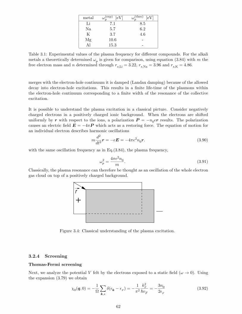
metal ω(exp)p [eV] ω(theo)

p [eV]

Li 7.1 8.5Na 5.7 6.2K 3.7 4.6

Mg 10.6 -Al 15.3 -

Table 3.1: Experimental values of the plasma frequency for different compounds. For the alkalimetals a theoretically determined ωp is given for comparison, using equation (3.84) with m thefree electron mass and n determined through rs,Li = 3.22, rs,Na = 3.96 and rs,K = 4.86.

merges with the electron-hole continuum it is damped (Landau damping) because of the alloweddecay into electron-hole excitations. This results in a finite life-time of the plasmons withinthe electron-hole continuum corresponding to a finite width of the resonance of the collectiveexcitation.

It is possible to understand the plasma excitation in a classical picture. Consider negativelycharged electrons in a positively charged ionic background. When the electrons are shifteduniformly by r with respect to the ions, a polarization P = −n0er results. The polarizationcauses an electric field E = −4πP which acts as a restoring force. The equation of motion foran individual electron describes harmonic oscillations

md2

dt2r = −eE = −4πe2n0r. (3.90)

with the same oscillation frequency as in Eq.(3.84), the plasma frequency,

ω2p =

4πe2n0

m. (3.91)

Classically, the plasma resonance can therefore be thought as an oscillation of the whole electrongas cloud on top of a positively charged background.

+r

Figure 3.4: Classical understanding of the plasma excitation.

3.2.4 Screening

Thomas-Fermi screening

Next, we analyze the potential V felt by the electrons exposed to a static field (ω → 0). Usingthe expansion (3.79) we obtain

χ0(q, 0) = − 1

Ω

∑k,s

δ(εk − εF ) = − 1

π2

k2F

~vF= −3n0

2εF

(3.92)

62

and thus

ε(q, 0) = 1 +k2TF

q2(3.93)

with the so-called Thomas-Fermi wave vector k2TF

= 6πe2n0/εF . The effect of the renormalizedq-dependence of the dielectric function can best be understood by considering a bare pointcharge Va(r) = e2/r (or Va(q) = 4πe2/q2) and its renormalization in momentum space

V (q) =Va(q)

ε(q, 0)=

4πe2

q2 + k2TF

(3.94)

or in real space

V (r) =e2

re−kTF r. (3.95)

The potential is screened by a rearrangement of the electrons and this turns the long-rangedCoulomb potential into a Yukawa potential with exponential decay. The new length scale is k−1

TF,

the so-called Thomas-Fermi screening length. In ordinary metals kTF

is typically of the sameorder of magnitude as k

F, i.e. the screening length is of order 5A comparable to the distance

between neighboring atoms.8 As a consequence also external electric fields cannot penetrate ametal, but are screened on this length 1/kTF . This legitimates one of the basic assumptionsused in electrostatics with metals.

Friedel oscillations

The static dielectric function can be evaluated exactly for a system of free electrons, resultingfor 3 dimensions in

ε(q, 0) = 1 +4e2mk

F

πq2

1

2+

4k2F− q2

8kFq

ln

∣∣∣∣2kF + q

2kF− q

∣∣∣∣ . (3.102)

8The Thomas-Fermi approach for electron gas is sketched in the following. The Thomas-Fermi theory forthe charge distributions slowly varying in space is based on the approximation that locally the electrons form aFermi gas with Fermi energy εF and electron density ne(εF ) neutralizing the ionic background. The electrostaticpotential Φ(r) of an external charge distribution ρex(r) induces a charge redistribution ρind(r) relative to ne(εF ).Within Thomas-Fermi approximation the induced charge distribution can then be written as

ρind(r) = −e[ne(εF + eΦ(~r))− ne(εF )

](3.96)

with

ne(εF ) =k3F

3π2=

1

3π2~2(2mεF )3/2 (3.97)

where εF = ~2k2F/2m. This approach is justified, if the spacial change of the potential Φ(r) is slow compared to

k−1F , so that locally we may describe the electron gas as a filled Fermi sphere of corresponding electron density.

The Poisson equation may now be formulated as

∇2Φ(r) = −4π[ρind(r) + ρex(r)] ≈ 4π

[e2Φ(r)

∂ne(ε)

∂ε

∣∣∣∣ε=εF

− ρex(r)

](3.98)

= k2TF Φ(r)− 4πρex(r) (3.99)

with the Thomas-Fermi momentum kTF defined as,

k2TF = 4πe2 ∂ne(ε)

∂ε

∣∣∣∣ε=εF

=6πe2neεF

. (3.100)

and ne = ne(εF ). For a point charge Q located at the origin we obtain,

Φ(r) = Qe−rkTF

r. (3.101)

This is the Yukawa potential as obtained above.

63

Noticeably the dielectric function varies little for small q kF

. At q = ±2kF

there is, however,a logarithmic singularity. This is a consequence of the sharpness of the Fermi surface in k-space.Consider the induced charge of a point charge at the origin: ena(r) = ena0δ(r) which is Fouriertransformed is na(q) = na0.9

δn(r) =

∫d3q

(2π)3

1

ε(q)− 1

na(q)eiq·r = −1

r

∞∫0

g(q)na(q) sin qr dq (3.104)

with

g(q) =q

2π2

ε(q)− 1

ε(q). (3.105)

Note that g(q) vanishes for both q → 0 and q →∞. Using partial integration twice, we find

δn(r) =na0

r3

∞∫0

g′′(q) sin qrdq (3.106)

where

g′(q) ≈ A ln|q − 2kF| (3.107)

and

g′′(q) ≈ A

q − 2kF

(3.108)

dominate around q ∼ 2kF

. Hence, for kF r 1,

δn(r) ≈ Ana0

r3

2kF+Λ∫2kF−Λ

sin[(q − 2kF

)r] cos 2kFr + cos[(q − 2k

F)r]sin2k

Fr

q − 2kF

dq (3.109)

−→ πAna0

cos 2kFr

r3. (3.110)

with a cutoff Λ→∞. The induced charge distribution exhibits so-called Friedel oscillations.Finally we may ask what is the total electron charge displaced around the point charge ena0δ(r).We take Eq.(charge-displace) and integrate over r.

δQ = eδn = e

∫d3r δn(r) = lim

q→0

1

ε(q)− 1

na(q) = −ena0 (3.111)

where we used 1/ε(q) → 0 for q → 0. The charge displacement corresponds to the exact op-posite amount of charge of of the point charge. Thus we find a perfect compensation whichcorresponds to perfect screening.

9The charge distribution can be deduced from the Poisson equation (3.65):

eδn(q) =q2

4πe2Vδn(q) = χ0(q, 0)V (q) = χ0(q, 0)

Va(q)

ε(q, 0)=

1− ε(q, 0)

ε(q, 0)na(q, 0) (3.103)

The charge distribution in real space can be obtained by Fourier transformation.

64

(Friedel oscillation)

i

r

Lindhard form

standard

Thomas−Fermin

Figure 3.5: Friedel oscillations of the charge distribution.

Dielectric function in various dimensions

Above we have treated the dielectric function for a three-dimensional parabolic band. Similarcalculations can be performed for one- and two-dimensional systems. In general, the staticsusceptibility is given by

χ0(q, ω = 0) =

− 1

2πqln

∣∣∣∣s+ 2

s− 2

∣∣∣∣ , 1D

− 1

2π

1−

(1− 4

s2

)1/2

θ(s− 2)

, 2D

− kF

2π2

1− s

4

(1− 4

s2

)ln

∣∣∣∣s+ 2

s− 2

∣∣∣∣ , 3D

(3.112)

where s = q/kF

. Interestingly χ0(q, 0) has a singularity at q = 2kF

in all dimensions. Thesingularity becomes weaker as the dimensionality is increased. In one dimension, there is alogarithmic divergence, in two dimensions there is a kink, and in three dimensions only thederivative diverges. Later we will see that these singularities may lead to instabilities of themetallic state, in particular for the one-dimensional case.

0

F

χ( ,0)q

χ(0,0)

3D

2D

1D

q

1

0 2k

Figure 3.6: Lindhard functions for different dimensions. The lower the dimension the strongerthe singularity at q = 2k

F.

65

3.3 Lattice vibrations - Phonons

The atoms in a lattice of a solid are not immobile but vibrate around their equilibrium positions.We will describe this new degree of freedom by treating the lattice as a continuous elastic medium(Jellium with elastic modulus λ). This approximation is sufficient to obtain some essentialfeatures of the interaction between lattice vibrations and electrons. In particular, renormalizedscreening effects will be found. Our approach here is, however, limited to mono-atomic unit cellsbecause the internal structure of a unit cell is neglected.

3.3.1 Vibration of a isotropic continuous medium

The deformation of an elastic medium can be described by the displacement of the infinitesimalvolume element d3r around a point r to a different point r′(r). We can introduce here theso-called displacement field u(r) = r′(r)− r as function of r. In general, u is also a function oftime. In the simplest form of an isotropic medium the elastic energy for small deformations isgiven by

Eel =λ

2

∫d3r (∇ · u(r, t))2 (3.113)

where λ is the elastic modulus (note that there is no deformation energy, if the medium isjust shifted uniformly). This energy term produces a restoring force trying to bring the systemback to the undeformed state. In this model we are neglecting the shear contributions.10 Thecontinuum form above is valid for deformation wavelengths that are much longer than the latticeconstant, so that details of the arrangement of atoms in the lattice can be neglected. The kineticenergy of the motion of the medium is given by

Ekin =ρ0

2

∫d3r

(∂u(r, t)

∂t

)2

(3.115)

where ρ0 = Mini is the mass density with the ionic mass Mi and the ionic density ni. Variationof the Lagrangian functional L[u] = Ekin − Eel with respect to u(r, t) leads to the equation ofmotion

1

c2s

∂2

∂t2u(r, t)−∇(∇ · u(r, t)) = 0, (3.116)

which is a wave equation with sound velocity c2s = λ/ρ0. The resulting displacement field can

be expanded into normal modes,

u(r, t) =1√Ω

∑k

ek

(qk(t)eik·r + qk(t)∗e−ik·r

)(3.117)

where every qk(t) satisfies the equation

d2

dt2qk + ω2

kqk = 0, (3.118)

10Note that the most general form of the elastic energy of an isotropic medium takes the form

Eel =

∫d3r

∑α,β=x,y,z

[λ

2(∂αuα)(∂βuβ) + µ(∂αuβ)(∂αuβ)

], (3.114)

where ∂α = ∂/∂rα. The Lame coefficients λ and µ characterize the elastic properties. The elastic constant λdescribes density modulations leading to longitudinal elastic waves, whereas µ corresponds to shear deformationsconnected with transversely polarized elastic waves. Note that transverse elastic waves are not important for thecoupling of electrons and lattice vibrations.

66

with the frequency ωk = cs|k| = csk and the polarization vector ek has unit length. Note thatwithin our simplification for the elastic energy (3.114), all modes correspond to longitudinalwaves, i.e. ∇ × u(r, t) = 0 and ek ‖ k. The total energy expressed in terms of the normalmodes reads

E =∑k

ρ0ω2k [qk(t)q∗k(t) + q∗k(t)qk(t)] . (3.119)

Next, we switch from a Lagrangian to a Hamiltonian description by defining the new variables

Qk =√ρ0(qk + q∗k) (3.120)

Pk =d

dtQk = −iωk

√ρ0(qk − q∗k) (3.121)

in terms of which the energy is given by

E =1

2

∑k

(P 2k + ω2

kQ2k

). (3.122)

Thus, the system is equivalent to an ensemble of independent harmonic oscillators, one for eachnormal mode k. Consequently, the system may be quantized by defining the canonical conjugateoperators Pk → Pk and Qk → Qk which obey, by definition, the commutation relation,

[Qk, Pk′ ] = i~δk,k′ . (3.123)

As it is usually done for quantum harmonic oscillators, we define the raising and loweringoperators

bk =1√

2~ωk

(ωkQk + iPk

)(3.124)

b†k =1√

2~ωk

(ωkQk − iPk

), (3.125)

satisfying the commutation relations

[bk, b†k′

] = δk,k′ , (3.126)

[bk, bk′ ] = 0, (3.127)

[b†k, b†k′

] = 0. (3.128)

These relations can be interpreted in a way that these operators create and annihilate quasi-particles following the Bose-Einstein statistics. According to the correspondence principle, thequantum mechanical Hamiltonian corresponding to the energy (3.122) is

H =∑k

~ωk

(b†kbk +

1

2

). (3.129)

In analogy to the treatment of the electrons in second quantization we say that the operators b†k(bk) create (annihilate) a phonon, a quasiparticle with well-defined energy-momentum relation,ωk = cs|k|. Using Eqs.(3.118, 3.121, and 3.125) the displacement field operator u(r) can nowbe defined as

u(r) =1√Ω

∑k

ek

√~

2ρ0ωk

[bke

ik·r + b†ke−ik·r

]. (3.130)

67

As mentioned above, the continuum approximation is valid for long wavelengths (small k) only.For wavevectors with k ≈ π/a the discreteness of the lattice appears in the form of correctionsto the linear dispersion ωk ∝ |k|. Since the number of degrees of freedom is limited to 3Ni (Ni

number of atoms), there is a maximal wave vector called the Debye wavevector11 kD

. We can nowdefine the corresponding Debye frequency ω

D= cskD and the Debye temperature Θ

D= ~ω

D/k

B.

In the continuous medium approximation there are only acoustic phonons. For the inclusion ofoptical phonons, the arrangement of the atoms within a unit cell has to be considered, whichgoes beyond this simple picture.

3.3.2 Phonons in metals

The consideration above is certainly valid for semiconductors, where ionic interactions are me-diated via covalent chemical bonds and oscillations around the equilibrium position may beapproximated by a harmonic potential, so that the form of the elastic energy above is well moti-vated. The situation is more subtle for metals, where the ions interact through the long-rangedCoulomb interaction and are held to together through an intricate interplay with the mobileconduction electrons.

First, neglecting the gluey effect of the electrons, the positively charged background can it-self be treated as an ionic gas. Similar to the electronic gas (3.84), the background exhibits awell-defined collective plasma excitation at the ionic plasma frequency

Ω2p =

4πni(Zie)2

Mi

, (3.131)

For equation (3.131) we used the formula (3.84) with n0 → ni = n0/Zi the density of ions withcharge number Zi, e → Zie, and m → Mi the atomic mass. Apparently the excitation energydoes not vanish as k → 0. So far, the background of the metallic system can not be describedas an elastic medium where the excitation spectrum is expected to be linear in k, ωk ∝ |k|.

The shortcoming in this discussion is that we neglected the feedback effects of the electrons thatreact nearly instantaneously to the slow ionic motion, due to their much smaller mass. Thefinite plasma frequency is a consequence of the long-range nature of the Coulomb potential (asmentioned earlier), but as we have seen above the electrons tend to screen these potentials, inparticular for small wavevectors k. The “bare” ionic plasma frequency Ωp is thus renormalizedto

ω2k =

Ω2p

ε(k, 0)=

k2Ω2p

k2 + k2TF

≈ (csk)2, (3.132)

where the presence of the electrons leads to a renormalization of the Coulomb potential by afactor 1/ε(k, ω). Having included the back-reaction of the electrons, a linear dispersion of asound wave (ωk = cs|k|) is finally recovered, and the renormalized velocity of sound cs reads

c2s ≈

Ω2p

k2TF

=Zmω2

p

Mik2TF

=1

3Zm

Mi

v2F . (3.133)

For the comparison of the energy scales we find,

ΘD

TF

∼ csvF

=

√1

3Zm

Mi

1, (3.134)

where we used kBTF

= εF

and kD≈ k

F.

11See course of Statistical Physics HS09.

68

Kohn anomaly

Notice that phonon frequencies are much smaller than the (electronic) plasma frequency, so thatthe approximation

ω2k =

Ω2p

ε(k, 0)(3.135)

is valid even for larger wavevectors. Employing the Lindhard form of ε(k, 0), we deduce thatthe phonon frequency is singular at |k| = 2k

F. More explicitly we find

∂ωk∂k→∞ (3.136)

in the limit k → 2kF

. This behavior is called the Kohn anomaly and results from the interactionbetween electrons and phonons. This effect is not contained in the previous elastic mediummodel that neglected ion-electron interactions.

3.3.3 Peierls instability in one dimension

The Kohn anomaly has particularly drastic effects in (quasi) one-dimensional electron systems,where the electron-phonon coupling leads to an instability of the metallic state. We consider aone-dimensional Jellium model where the ionic background is treated as an elastic medium with adisplacement field u along the extended direction (x-axis). We neglect both the electron-electroninteraction and the slow time evolution of the background modulation so that the Hamiltonianreads,

H = Hisol +Hint, (3.137)

where contributions of the isolated electronic and ionic systems are included in

Hisol =∑k,s

~2k2

2mc†k sck s +

λ

2

∫dx

(du

dx(x)

)2

(3.138)

whereas the interactions between the system comes in via the coupling

Hint = −n0

∑s

∫dx dx′ V (x− x′) d

dxu(x)Ψ†s(x

′)Ψs(x′) (3.139)

In the general theory of elastic media ∇ · u = −δn/n0 describes density modulations, so thatthe second term in (3.137) models the coupling of the electrons to charge density fluctuations ofthe positively charged background12 mediated by the screened Coulomb interaction V (x − x′).Consider the ground state of N electrons in a system of length L, leading to an electronic densityn0 = N/L. For a uniform background u(x) = const, the Fermi wavevector of free electrons isreadily determined to be

N =∑s

L

2π

+kF∫−kF

dk 1 = 2L

2π2k

F(3.140)

leading to

kF

=π

2n0. (3.141)

12Note that only phonon modes with a finite value of ∇ ·u couple in lowest order to the electrons. This is onlypossible of longitudinal modes. Transverse modes are defined by the condition ∇ · u = 0 and do not couple toelectrons in lowest order.

69

Perturbative approach - instability

Now we consider the Kohn anomaly of this system. For a small background modulation u(x) 6=const, the interaction term Hint can be treated perturbatively and will lead to a renormalizationof the elastic modulus λ in (3.137). For that it will be useful to express the full Hamiltonian inmomentum space,

Hisol =∑k,s

~2k2

2mc†k sck s +

Ωρ0

2

∑q

ω2ququ−q (3.142)

Hint = i∑k,q,s

q[V−quq c

†k+q,sck,s − Vqu−q c

†k,sck+q,s

], (3.143)

where we used from previous considerations λq2 = ρ0ω2q . Furthermore we defined

u(x) =1√L

∑q

uqeiqx, (3.144)

V (x) =1√L

∑q

Vqeiqx, (3.145)

with Vq = 4πe2/q2ε(q, 0) ≈ const. - we consider an effectively short-ranged potential. Wecompute the second order correction to the ground state energy using Rayleigh-Schrodingerperturbation theory (note that the linear energy shift vanishes)

∆E(2) =∑k,q,s

q2|Vq|2uqu−q∑n

|〈Ψ0|c†k,sck+q,s|n〉|2 + |〈Ψ0|c

†k+q,sck,s|n〉|2

E0 − En(3.146)

=∑q

|Vq|2q2uqu−q∑k

nk+q − nkεk+q − εk

(3.147)

= Ω∑q

|Vq|2q2χ0(q, 0)uqu−q (3.148)

where the virtual states |n〉 are electron-hole excitations of the filled Fermi sea. This term givesa correction to the elastic term in (3.142). In other words, the elastic modulus λ and, thus, thephonon frequency ωq

2 = λ/ρ0q2 = c2

sq2 is renormalized according to

(ωrenq

)2 ≈ ω2q +|Vq|2q2

ρ0

χ0(q, 0) = ω2q −|Vq|2q2πρ0

ln

∣∣∣∣q + 2kF

q − 2kF

∣∣∣∣ (3.149)

From the behavior for q → 0 we infer that the velocity of sound is renormalized. However, a muchmore drastic modification occurs at q = 2k

F. Here the phonon spectrum is ’softened’, i.e. the

frequency vanishes and even becomes negative. The latter effect is an artifact of the perturbationtheory.13 This hints at an instability triggered by the Bose-Einstein condensation of phononswith a wave vector of q = 2k

F. This coherent superposition14 of many phonons corresponds

classically to a static periodic deformation of the ionic background with wave vector 2kF

. Theunphysical behavior of the frequency ωq indicates that in the vicinity of 2k

F, the current problem

can not be treated with the help of perturbation theory around the uniform state.

13Note that indeed the expression

ω2q =

Ω2p

ε(q, 0)(3.150)

in (3.135) does not yield negative energies but gives a zero of ωq at q = 2kF .14We introduce the coherent state

|ΦcohQ 〉 = e−|α|

2/2∞∑n=0

(b†Q)n

n!αn|0〉 (3.151)

70

q

q

2k F

ωq(ren)

ω

Figure 3.7: Kohn anomaly for the one-dimensional system with electron-phonon coupling. Therenormalization of the phonon frequency is divergent at q = 2k

F.

Peierls instability at Q = 2kF

Instead of the perturbative approach, we assume that the background shows a periodic densitymodulation (coherent phonon state)

u(x) = u0 cos(Qx) (3.154)

where Q = 2kF

and u0 remains to be determined variationally. We investigate the effect ofthis modulation on the electron-phonon system. To this end we show that such a modulationlowers the energy of the electrons. Assuming that u0 is small we can evaluate the electronicenergy using the approximation of nearly free electrons, where Q appears as a reciprocal latticevector. The electronic spectrum for 0 ≤ k ≤ Q is then approximately determined by the secularequation

det

(~2k2

2m − E ∆

∆∗ ~2(k−Q)2

2m − E

)= 0 (3.155)

where ∆ follows from the Fourier transform of the potential V (x),

∆ = −iQu0nVQ (3.156)

with

VQ =

∫dx eiQxV (x). (3.157)

The equation (3.155) leads to the energy eigenstates

E±k =~2

4m

[(k −Q)2 + k2 ±

√(k −Q)2 − k22 + 16m2|∆|2/~4

]. (3.158)

which does not have a definite phonon number for the mode of wave vector Q. On the other hand, this mode ismacroscopically occupied, since

nQ = 〈ΦcohQ |b†QbQ|Φcoh

Q 〉 = |α|2 (3.152)

and, moreover, we find

〈ΦcohQ |u(x)|Φcoh

Q 〉 =1

L

~2ρ0ωQ

[αeiQx + α∗e−iQx

]= u0 cos(Qx) (3.153)

with u0 = ~α/ρ0LωQ, assuming α being real.

71

The total energy of the electronic and ionic system is then given by

Etot(u0) = 2∑

0≤k<QEk− +

λLQ2

4u2

0 (3.159)

where all electronic states of the lower band (Ek−) are occupied and all states of the upper band(Ek+) are empty. The amplitude u0 of the modulation is found by minimizing Etot with respectto u0:

0 =1

L

dEtot

du0

(3.160)

= − ~2

2m

32Q2m2n2V 2Q

~4u0

Q∫0

dk

2π

1√(k −Q)2 − k22 + 16m2Q2n2V 2

Qu2

0/~4+λ

2Q2u0 (3.161)

= −u0

4Qmn2V 2Q

~2π

+kF∫−kF

dq1√

q2 + 4m2n2V 2Qu2

0/~4+λ

2Q2u0 (3.162)

= −u0

8Qmn2V 2Q

~2πarsinh

(~2k

F

2mnVQu0

)+λ

2Q2u0. (3.163)

We solve this equation for u0 using arsinh(x) ≈ ln(2x) when x 1.

u0 =~2k

F

mnVQ

exp

[− ~2k

Fπλ

8mn2V 2Q

]=

2

kF

εF

nVQ

e−1/N(0)g (3.164)

where εF

= ~2k2F/2m is the Fermi energy and N(0) = 2m/π~2k

Fis the density of states at the

Fermi energy. We introduced the coupling constant g = 4n2V 2Q/λ that describes the phonon-

induced effective electron-electron interaction. The coupling is the stronger the more polarizable(softer) ionic background, i.e. when the elastic modulus λ is small. Note that the static displace-ment u0 depends exponentially on the coupling and on the density of states. The underlyingreason for this so-called Peierls instability to happen lies in the opening of an energy gap,

∆E = E+kF− E−kF = 2|∆| = 8ε

Fexp

(− 1

N(0)g

), (3.165)

at k = ±kF

, i.e. at the Fermi energy. The gap is associated with a lowering of the energy of theelectron states in the lower band in the vicinity of the Fermi energy. For this reason this kindof instability is called a Fermi surface instability. Due to the gap the metal has turned into asemiconductor with a finite energy gap for all electron-hole excitations.The modulation of the electron density follows the charge modulation due to the ionic latticedeformation, which can be seen by expressing the wave function of the electronic states,

ψ′k(x) =1√Ω

∆eikx + (Ek − εk)ei(k−Q)x√(Ek − εk)2 + |∆|2

, (3.166)

which is a superposition of two plane waves with wave vectors k and k−Q, respectively. Hencethe charge density reads

ρk(x) = −e|ψ′k(x)|2 = − eΩ

[1− 2(εk − Ek)|∆|

(Ek − εk)2 + |∆|2 sinQx

](3.167)

72

µ

E E

kk +Q−Q

Figure 3.8: Change of the electron spectrum. The modulation of the ionic background yieldsgaps at the Fermi points and the system becomes an insulator.

and its modulation from the homogeneous distribution −en is given by

δρ(x) =∑k

ρk(x)− (−en) =e

2

kF∫0

dk′

2π

m|∆| sinQx√~4k2

Fk′2 +m2|∆|2

(3.168)

=en|∆|16ε

F

ln

∣∣∣∣2εF|∆|∣∣∣∣ sin(2k

Fx). (3.169)

Such a state, with a spatially modulated electronic charge density, is called a charge densitywave (CDW) state. This instability is important in quasi-one-dimensional metals which are forexample realized in organic conductors such as TTF·TCNQ (tetrathiafulvalene tetracyanoquino-methane). In higher dimensions the effect of the Kohn anomaly is generally less pronounced, sothat in this case spontaneous deformations rarely occur. As we will see later, a charge densitywave instability can nevertheless be observed in multi-dimensional (d > 1) systems with a so-called nested Fermi surface. These systems resemble in some respects one-dimensional systems.Finally, notice that the electron-phonon interaction strongly contributes to another kind of Fermisurface instability, when metals exhibit superconductivity.

3.3.4 Dynamics of phonons and the dielectric function

We have seen that an external potential Va is screened by the polarization of the electrons.As the positively charged ionic background is also polarizable, it should be included in therenormalization of the external potential. In general, the fully renormalized potential Vren maybe expressed via

εVren = Va, (3.170)

with the full dielectric function ε. In order to determine Vren and ε, we define the ’bare’ (unrenor-malized) electronic (ionic) dielectric function εel (εion). The renormalized potential in (3.170)can be expressed considering three other points of view. First, if the ionic potential Vion is addedto the external potential Va, the remaining screening is due to the electrons only, i.e.,

εelVren = Va + Vion. (3.171)

Secondly, the electronic potential Vel may be added to the external potential Va, so that the ionsexclusively renormalize the new potential Vel + Va, resulting in

εionVren = Va + Vel. (3.172)

Note that in (3.172) all effects of electron polarization are included in Vel, so that the dielectricfunction results from the ’bare’ ions. Finally we use the fact that Vren may be expressed as

Vren = Va + Vel + Vion. (3.173)

73

Adding (3.171) to (3.172) and subtracting (3.170), we obtain

(εel + εion − ε)Vren = Va + Vel + Vion (3.174)

which simplifies with (3.173) to

ε = εel + εion − 1 (3.175)

In order to find an alternative expression relating the renormalized potential Vren to the externalpotential Va, we make the Ansatz

Vren =1

εVa =

1

εioneff

1

εelVa (3.176)

i.e. the potential Va/εel that results from bare screening of the polarizable electrons is addi-

tionally screened by an effective ionic dielectric function εioneff which includes electron-phonon

interactions. Using equation (3.175) and the definition of εioneff via (3.176) we obtain

εioneff = 1 +

1

εel(εion − 1), (3.177)

or using the definition (3.70)

χion0,eff =

χion0

εel. (3.178)

Taking into account the discussion of the plasma excitation of the bare ions in Eqs.(3.83, 3.84,and 3.131), and considering the long wave-length excitations (k→ 0), we approximate

εion = 1−Ω2p

ω2, (3.179)

εel = 1 +k2TF

k2. (3.180)

For the electrons we used the result from the quasi-static limit in (3.93). The full dielectricfunction now reads

ε = 1 +k2TF

k2−

Ω2p

ω2=

(1 +

k2TF

k2

)(1− ω2

k

ω2

). (3.181)

ε+ω

’ ε−ω’

q,

k, k+q,

k’−q,k’,

ε

ε

Figure 3.9: Diagram for the electron-electron interaction involving also electron-phonon cou-pling.

74

The time-independent Coulomb interaction

Va =4πe2

q2(3.182)

between the electrons is replaced in a metal by an effective interaction

Vren(q, ω) =4πe2

q2ε(q, ω)(3.183)

=4πe2

k2TF

+ q2

(ω2

ω2 − ω2q

). (3.184)

This interaction corresponds to the matrix element for a scattering process of two electronswith momentum exchange q and energy exchange ω. The phonon frequency ωq is always lessthan the Debye frequency ω

D. Hence the effect of the phonons is almost irrelevant for energy

exchanges ω that are much larger than ωD

. The time scale for such energies would be too shortfor the slow ions to move and influence the interaction. Interestingly, the repulsive bare Coulombpotential is renormalized to an interaction with an attractive channel for ω < ω

Dbecause of

overcompensation by the ions. This aspect of the electron-phonon interaction is most importantfor superconductivity.

75

Chapter 4

Itinerant electrons in a magneticfield

Electrons couple through their orbital motion and their spin to external magnetic fields. Inthis chapter we focus on the case of orbital coupling which can be also used as a diagnostictool to observe the presence of a Fermi surface in a metallic system and to map out the Fermisurface topology. A further most intriguing feature of electrons moving in a magnetic field isthe Quantum Hall effect of a two-dimensional electronic system. In both case the Landau levelswith play an important role and will be introduced here in a first step.

4.1 The de Haas-van Alphen effect

The ground state of a metal is characterized by the existence of a discontinuity of the occupationnumber in momentum space - the Fermi surface. The de Haas-van Alphen experiment is oneof the best methods to verify its existence and to determine the shape of a Fermi surface. It isbased on the behavior of electrons at low temperatures in a strong magnetic field.

4.1.1 Landau levels

Consider a free electron gas subject to a uniform magnetic field B = (0, 0, B). The one-particleHamiltonian for an electron is given by

H =1

2m

(−i~∇− e

cA)2− gµ

B

~SzB. (4.1)

We fix the gauge freedom of the vector potential A by working in the Landau gauge, A =(0, Bx, 0), satisfying B = ∇×A. Hence the Hamiltonian (4.1) simplifies to

H =1

2m

[−~2 ∂

2

∂x2+

(−i~ ∂

∂y− e

cBx

)2

− ~2 ∂2

∂z2

]− gµ

B

~SzB. (4.2)

In this gauge, the vector potential acts like a confining harmonic potential along the x-axis. Astranslational invariance in the y- and z-directions is preserved, the eigenfunctions separate inthe three spacial components and take the form

ψ(r) = eikzzeikyyφ(x)ξs (4.3)

where ξs is the spin wave function. The states φ(x) are found to be the eigenstates of theharmonic oscillator problem, so that we have

φn,ky(x) =1√

2n n! 2π `2Hn[(x− ky`2)/`]e−(x−ky`2)2/2`2 (4.4)

76

where Hn(x) are the Hermite polynomials and ` represents the magnetic length defined via`2 = ~c/|eB|. The eigenenergies of the Hamiltonian (4.2) read

En,kz ,s =~2k2

z

2m+ ~ωc

(n+

1

2

)− gµ

B

~Bs (4.5)

where s = ±~/2, n ∈ N0 and we have introduced the cyclotron frequency ωc = |eB|/mc. Notethat the energy (4.5) does not depend on ky. The apparent differences in the spatial dependence

of the wave functions for the x- and y-directions are merely a consequence of the chosen gauge.1

The fact that the energy does not depend on ky in the chosen gauge indicates a huge degeneracyof the eigenstates. To obtain the number of degenerate states we concentrate for simplicity onkz = 0 and neglect the electron spin. We take the electrons to be confined to a cube of volumeL3 with periodic boundary conditions, i.e., ky = 2πny/L with ny ∈ N0. As the wave function

φn,ky(x) is centered around ky`2, the condition

0 < ky`2 < L (4.8)

fixes the maximal number Ndeg of degenerate states

0 < ny < Ndeg =L2

2π`2=L2B

hc/e=

Φ

Φ0

. (4.9)

where Φ0 = hc/e is the magnetic flux quantum (e.g. Aharonov-Bohm interference effect). Thusthe degeneracy Ndeg corresponds to the number of flux quanta included in the total magneticflux Φ threading the system.The energies correspond to a discrete set of one-dimensional systems, so that the density of statesis determined by the structure of the one-dimensional dispersion (with square root singularitiesat the band edges) along the z-direction:

N0(E,n, s) =Ndeg

Ω

∑kz

δ(E − En,kz ,s) (4.10)

=1

2π`2

∫dkz2π

δ

(E − ~2k2

z

2m− ~ωc

(n+

1

2

)+gµ

B

~Bs

)(4.11)

=(2m)3/2ωc

8π2~2

1√E − ~ωc(n+ 1/2) + gµ

BBs/~

(4.12)

The total density of states N0(E) for a given energy E is obtained by summing over n ∈ N0 ands = ±~/2. This should be compared to the density of states without the magnetic field,

N0(E,B = 0) =1

Ω

∑k,s

δ

(E − ~2k2

2m

)=

(2m)3/2

2π2~3

√E . (4.13)

The density of states for finite applied field is shown in Fig. 4.1 for one spin-component.

1Like the vector potential, the wave function is a gauge dependent quantity. To see this, observe that under agauge transformation

A(r, t)→ A′(r, t) = A(r, t) + ∇χ(r, t) (4.6)

the wave function undergoes a position dependent phase shift

ψ(r, t)→ ψ′(r, t) = ψ(r, t)ei~cχ(r,t)/e. (4.7)

77

B=00

B=0E

N

Figure 4.1: Density of states for electrons in a magnetic field due to Landau levels. The dashedline shows the density of states in the absence of a magnetic field.

4.1.2 Oscillatory behavior of the magnetization

In the presence of a magnetic field, the smooth density of states of the three-dimensional metalis replaced by a discontinuous form dominated by square root singularities. The position of thesingularities depends on the strength of the magnetic field. In order to understand the resultingeffect on the magnetization, we consider the free energy

F = Nµ− TS = Nµ− kBT

∑kz ,ky ,n,s

ln(

1 + e−(En,kz,s−µ)/kBT)

(4.14)

and use the general thermodynamic relation M = −∂F/∂B. For the details of the somewhattedious calculation, we refer to J. M. Ziman, Principles of the Theory of Solids2 and merelypresent the result

M = NχPB

1 +χL

χP

+πk

BT

µBB

√εF

µBB

∞∑ν=1

1√ν

sin(π4 −

πνεFµBB

)sinh

(π2νkBTµBB

) . (4.15)

Here χP

is the Pauli-spin susceptibility originating from the Zeeman-term and the second termχL

= −χP/3 is the diamagnetic Landau susceptibility which is due to induced orbital currents

(the Landau levels). For sufficiently low temperatures, kBT < µ

BB ∼ ~ωc, the magnetization as

a function of the applied field exhibits oscillatory behavior. The dominant contribution comesfrom the summand with ν = 1. The oscillations are a consequence of the singularities in thedensity of states that influence the magnetic moment upon successively passing through theFermi energy as the magnetic field is varied. The period in 1/B of the oscillations of the termν = 1 is easily found to be

πεF

µB

∆

(1

B

)= 2π (4.16)

or

∆

(1

B

)=

2πe

~c1

A(kF

)(4.17)

where we used that µB

= ~e/2mc and defined the cross sectional area A(kF

) = πk2F

of the Fermisphere perpendicular to the magnetic field.

2German title : Prinzipien der Festkorpertheorie

78

4.1.3 Onsager equation

The behavior we have found above for a free electron gas, generalizes to systems with arbitraryband structures. In these cases there are usually no exact solutions available. Instead of gener-alizing the above treatment to such band systems, we discuss the behavior of electrons withinthe semiclassical approximation, as introduced in Section 1.7, and consider the closed orbits ofa wave packet subject to a magnetic field. The semiclassical equations of motion for the centerof mass of the wave packet (1.96, 1.97) simplify in the absence of an electric field to

r = vk =∂εk∂~k

(4.18)

~k = −ecvk ×B. (4.19)

This defines a closed path in a plane perpendicular to the applied uniform field. Hence, we canapply the Bohr-Sommerfeld quantization scheme yielding quantized closed paths Pn ,∮

Pn

p · dr = h(n+ γ) (4.20)

with n being an integer and γ a system specific shift, irrelevant for the final result and h = 2π~.The momentum within the semiclassical approach is expressed as

p = ~k − e

cA = −e

c(r ×B +A) , (4.21)

where we used Eq.(4.19) integrated over time. Thus, Eq.(4.20) can be now evaluated as∮Pn

p · dr = −ec

∮Pn

r ×B +A · dr = fracecΦn +e

cB ·

∮Pn

r × dr︸ ︷︷ ︸=2eB⊥Sn/c=2eΦn/c

= h(n+ γ) , (4.22)

where Sn is the area encircled by the path Pn and Φn = B⊥Sn the magnetic flux threading.With this we find

Φn = (n+ γ)Φ0 . (4.23)

Now we compare the areas of a given trajectory in real and reciprocal space, Sn andAn,respectively.Considering ~k = e(r ×B)/c yields

|dr| = Φ0

2πB⊥|dk| ⇒ Sn =

(Φ0

2πB⊥

)2

An (4.24)

With the flux quantization in Eq.(4.23) we obtain for a given magnetic field the area An,

An = (n+ γ)4π2B⊥Φ0

(4.25)

while for a given area A we obtain,

A = (n+ γ)4π2BnΦ0

= (n′ + γ)4π2

Φ0

Bn′ . (4.26)

Thus changing the field B by a certain amount Bn → Bn+1 would yield the same A and oneperiod of chaning density of states, i.e. magnetization. From this we conclude that there is aregular oscillation as a function of 1/B and the period is connected with the area A,

∆

(1

B

)=

1

Bn+1

− 1

Bn=

4π2

AΦ0

. (4.27)

79

Fermisurface

extremalarea

extremalareas

band botton

band botton

band top

Figure 4.2: Concentric tubes represent the quantized orbits in the reciprocal space correspondingto the areas An embedded in the original Fermi surface which limits the height of the tubes,occupation along the k‖-direction (k‖ ‖ B). Left panel: 3-dimensional view of system with asimple Fermi surface. Right panel: cross section including k‖. Extremal areas represent theband edges (bottom: maximal A; and top: minimal A).

As we have seen above (Eq.(4.12)) the Fermi energy passes through a singularity in the densityof states at the band bottom of the one-dimensional motion of the electrons along kz or k‖ ‖ B.This corresponds the extremal area A(k‖). Note, also a band top yields the same type ofsingularity and corresponds to a minimum of A(k‖). Therefore, in experiment the magnetizationmaxima oscillate with a period in the inverse magnetic field as given by Eq.(4.27).The oscillations in the magnetization, thus, allow to measure the cross sectional area of theFermi ’sphere’. By varying the orientation of the field the topology of the Fermi surface canbe mapped. As an alternative to the measurement of magnetization oscillations one can alsomeasure resistivity oscillations known under the name Schubnikov-de Haas effect. For bothmethods it is crucial that the Landau levels are sufficiently clearly recognizable. Apart fromlow temperatures this necessitates sufficiently clean samples. In this context, sufficiently cleanmeans that the average life-time τ (average time between two scattering events) has to be muchlarger than the period of the cyclotron orbits, i.e. ωcτ 1. This condition follows from theuncertainty relation

∆ε ∼ ~τ ~ωc. (4.28)

4.2 Quantum Hall Effect

Classical Hall Effect

The Hall effect, discovered by Edwin Hall in 1879, originates from the Lorentz force exerted bya magnetic field on a moving charge. This force is perpendicular both to the velocity of thecharged particle and to the magnetic field. In the presence of an electrical current, a Lorentzforce produces a transverse voltage, whenever the applied magnetic field points in a directionnon-collinear to the current in the conductor. This so-called Hall effect can be used to investigatesome properties of the charge carriers. Before treating the quantum version, we briefly review

80

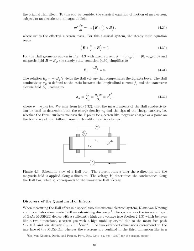
the original Hall effect. To this end we consider the classical equation of motion of an electron,subject to an electric and a magnetic field

m∗dv

dt= −e

(E +

v

c×B

), (4.29)

where m∗ is the effective electron mass. For this classical system, the steady state equationreads (

E +v

c×B

)= 0. (4.30)

For the Hall geometry shown in Fig. 4.3 with fixed current j = (0, jy, 0) = (0,−n0ev, 0) andmagnetic field B = Bz, the steady state condition (4.30) simplifies to

Ex +vBzc

= 0. (4.31)

The solution Ex = −vBz/c yields the Hall voltage that compensates the Lorentz force. The Hallconductivity σ

His defined as the ratio between the longitudinal current jy and the transverse

electric field Ex, leading to

σH

=jyEx

=n0ec

Bz= ν

e2

h, (4.32)

where ν = n0hc/Be. We infer from Eq.(4.32), that the measurements of the Hall conductivitycan be used to determine both the charge density n0 and the sign of the charge carriers, i.e.whether the Fermi surfaces encloses the Γ-point for electron-like, negative charges or a point onthe boundary of the Brillouin zone for hole-like, positive charges.

V

yV

B z

x

I

x

y

Figure 4.3: Schematic view of a Hall bar. The current runs a long the y-direction and themagnetic field is applied along z-direction. The voltage Vy determines the conductance alongthe Hall bar, while Vx corresponds to the transverse Hall voltage.

Discovery of the Quantum Hall Effects

When measuring the Hall effect in a special two-dimensional electron system, Klaus von Klitzingand his collaborators made 1980 an astonishing discovery.3 The system was the inversion layerof GaAs-MOSFET device with a sufficiently high gate voltage (see Section 2.4.3) which behaveslike a two-dimensional electron gas with a high mobility eτ/m∗ due to the mean free pathl ∼ 10A and low density (n0 ∼ 1011cm−2. The two extended dimensions correspond to theinterface of the MOSFET, whereas the electrons are confined in the third dimension like in a

3See [von Klitzing, Dorda, and Pepper, Phys. Rev. Lett. 45, 494 (1980)] for the original paper.

81

potential well (cf. Section 2.4.3). In high magnetic fields between 1 − 30T and at sufficientlylow temperatures (T < 4K), von Klitzing and coworkers observed a quantization of the Hallconductivity corresponding to exact integer multiples of e2/h

σH

= νne2

h(4.33)

where νn ∈ N. By now, the integer quantization is so widely verified, that the von Klitzingconstant (resistance quantum named after the discoverer of the Quantum Hall effect) R

K=

h/e2 = 25812.807557Ω is used in resistance calibrations. In the field range where the transverseconductivity shows integer plateaus in ν ∝ 1/B, the longitudinal conductivity σyy vanishes andtakes finite values only when σ

Hcrossed over from one quantized value to the next (see Fig.

4.4).

ν

2σ

xyσ

yy

1

2

3

1 320

0ν

/ (e

/

h )

Figure 4.4: Integer Quantum Hall effect: As a function of the filling factor ν plateaus in σxyappear at multiples of e2/h. The longitudinal conductance σyy is only finite for fillings whereσxy changes between plateaus.

In 1982, Tsui, Stormer, and Gossard4 discovered an additional quantization of σH

, correspondingto certain rational multiples of e2/h. Correspondingly, one now distinguishes between the integerquantum Hall effect (IQHE) and the fractional quantum Hall effect (FQHE). These discoveriesmarked the beginning of a whole new field in solid state physics that continues to produceinteresting results.

4.2.1 Hall effect of the two-dimensional electron gas

Here we first discuss the Hall effect in the quantum mechanical treatment. For this purposewe start with the Hamilton operator (4.1) and neglect the electron spin. Working again inthe Landau gauge, A = (0, Bx, 0), and confining the electronic system to two dimensions, theHamiltonian reduces to

H =1

2m

[−~2 ∂

2

∂x2+

(−i~ ∂

∂y+e

cBx

)2]. (4.34)

For the two-dimensional gas there is no motion in the z-direction, so that the highly degenerateenergy eigenvalues are given by the spectrum of a one-dimensional harmonic oscillator En =~ωc(n+ 1/2), where again ωc = |eB|/m∗c. Here, we will concentrate on the lowest Landau level

4See [Tsui, Stormer and Gossard Phys. Rev. Lett. 48, 1559 (1982)] for the original paper

82

(n = 0) with the wave function

φ0,ky=

1√2π`2

e−(x−x0)2/2`2eikyy. (4.35)

where the magnetic length ` =√

~c/|eB| gives the extension of the wave function in the presenceof the magnetic field. In x-direction, the wave function is localized around x0 = −ky`2, whereasit takes the form of a plane wave in y-direction. As discussed previously, the energy does notdepend on ky.

We now introduce an electric field Ex along the x-direction. The Hamilton operator (4.34) isthen modified by an additional potential U(r) = −eExx. This term can easily be absorbed intothe harmonic potential and leads to a shift of the center of the wave function,

x0(ky)→ x′0(ky) = −ky`2 −eExm∗ω2

c

. (4.36)

Moreover the degeneracy of the Landau level is lifted since the energy becomes ky-dependentand (after completing the square) takes the form

En=0(ky) =~ωc2

+ eExx′0(ky) +

m∗

2

(cExB

)2

. (4.37)

The energy (4.37) corresponds to the wave function φ0kyfrom (4.35) where x0 is replaced by x′0.

The velocity of the electrons is then given by

vy(ky) =1

~dEn=0(ky)

dky= −eEx`

2

~= −cEx

B, (4.38)

and from this, we determine the current density,

jy = −en0vy(ky) = en0

cExB

=eν

2π`2cExB

= νe2

hEx = σ

HEx (4.39)

where ν = n02π`2 is the filling of the Landau level.5 The Hall conductivity is then identical tothe result (4.32) derived previously based on the quasiclassical approximation. There is a linearrelation between the Hall conductivity σ

Hand the index ν ∝ B−1.

4.2.2 Integer Quantum Hall Effect

The plateaus observed by von Klitzing in the Hall conductivity σH

of the two-dimensionalelectron gas as a function of the magnetic field correspond to the values σ

H= νne

2/h, as ifν = νn ∈ N was restricted to be an integer. Meanwhile, the longitudinal conductivity of theelectron gas vanishes when a plateau of σ

His realized

σyy =jyEy

= 0, (4.40)

and only becomes finite at the transition points of σH

between two plateaus (cf. Fig. 4.4). Thisfact seems to be in contradiction with the results from the consideration above. The solutionto this mysterious behavior lies in the fact that disorder, which is always present in a realinversion layer, plays a crucial role and should not be neglected. In fact, due to the disorder, theelectrons move in a randomly modulated potential landscape U(x, y). As we will find out, evensmall amounts of disorder lead to the localization of electronic states in this two-dimensional

5Note that ν−1 = B/n0Φ0 where Φ0 = hc/e represents the flux quantum, i.e. ν−1 ∝ B is the number of fluxquanta Φ0 per electron.

83

system. To illustrate this new aspect we focus on the lowest Landau level in the symmetricgauge A = (−y, x, 0)B/2. The Schrodinger equation in polar coordinates is given by

~2

2m∗

[−1

r

∂

∂rr∂

∂r−(

1

r

∂

∂ϕ− i e

2~cBr

)2]ψ(r, ϕ) + U(x, y)ψ(r, ϕ) = Eψ(r, ϕ) . (4.41)

Without the external potential U(x, y) we find the ground state solutions

ψn=0,m(r, ϕ) =1√

2π`22mm!

(r`

)me−imϕe−r

2/4`2 (4.42)

where all values of m ∈ N0 correspond to the same energy En=0 = ~ωc/2. One easily verifies,that the wave functions |ψn=0,m(r, ϕ)| are peaked on circles of radius rm =

√2m` (see Fig.4.5).

Note that the magnetic flux threading such a circle is given by

πBr2m = πB2m`2 = 2πmB

~ceB

= mhc

e= mΦ0, (4.43)

which is an integer multiple of the flux quantum Φ0 = hc/e.

x y

|ψ|2

Figure 4.5: Wavefunction of a Landau level state in the symmetric gauge.

Now we consider the effect of the disorder potential. The gauge can be adjusted to the potentiallandscape. If, for simplicity, we assume the potential to be rotationally invariant around theorigin, the symmetric gauge is already optimal. For the potential

U(x, y) = U(r) =C1

r2+ C2r

2 + C3, (4.44)

the exact expression of all eigenstates of equation (4.41) in the lowest Landau level is obtainedusing the Ansatz

ψ0,m(r, ϕ) =1√

2π`∗22αΓ(α+ 1)

( r`∗

)αe−imϕe−r

2/4`∗2 . (4.45)

After introducing the dimensionless parameters C∗1 = 2m∗C1/~2 and C∗2 = 8`4m∗C2/~2, thequantities α and `∗ from equation (4.45) can be expressed via

α2 = m2 + C∗1 , (4.46)(`∗)−2

=(`)−2√

1 + C∗2 . (4.47)

Indeed, the Ansatz (4.45) describes eigenstates of the disordered problem (4.41). The degeneracyof the ground state energy (the lowest Landau level) is now lifted,

E0,m =~ωc2

[`2

`∗2(α+ 1)−m

]+ C3. (4.48)

84

The wave functions are concentrated around the radii rm =√

2α`∗. For weak potentialsC∗1 , C

∗2 1 and m 1 the energy is approximatively given by

E0,m ≈~ωc2

+C1

r2m

+ C2r2m + C3 + . . . , (4.49)

i.e. the wave function adjusts itself to the potential landscape. It turns out that the same is truefor arbitrarily structured weak potential landscapes. The wave function describes electrons onquasi-classical trajectories that trace the equipotential lines of the underlying disorder potential.Consequently the states described here are localized in the sense that they are attached to thestructure of the potential. The application of an electric field cannot set the electrons in theconcentric rings in motion. Therefore, the electrons are localized and do not contribute toelectric transport.

Picture of the potential landscape

When the magnetic field is varied the filling ν = n02π`2 of the Landau level is adjusted accord-ingly. While all states of a given level are degenerate in the transitionally invariant case, now,these states are spread over a certain energy range due to the disorder. In the quasi-classical ap-proximation, these states correspond to equipotential trajectories that are either filled or emptydepending on the strength of the magnetic field, i.e. they are either below or above the chemicalpotential. These considerations lead to an intuitive picture on localized (closed trajectories) andextended (percolating trajectories) states. We may consider the potential landscape like a reallandscape where the the trajectories are contour lines. Assume that we fill now water into sucha landscape. The trajectories of the particles is restricted to the shore line. For small filling, wefind lakes whose shores are closed and correspond to contour lines. They correspond to closedelectron trajectories and represent localized electronic states. At very high water level, onlythe large mountains of the potential landscape would reach out of the water, forming islands inthe sea. The coastlines again represent closed trajectories corresponding to localized electronicstates. At some intermediate filling, a boundary between the lake and the island topology,there is a water level at which the coast lines become arbitrarily long and percolate throughthe whole landscape. Only these contour lines correspond to extended (non-localized) electronstates. From this picture we conclude that when a Landau level of a system subject to a randompotential is gradually filled, first all occupied state are localized (low filling). At some special in-termediate filling level, the extended states are filled and contribute to the current transport. Athigher chemical potential (filling) the states would be localized again. In the following argument,going back to Robert B. Laughlin, the presence of filled extended states plays an important role.

Laughlin’s gauge argument

We consider a long rectangular Hall element that is deformed into a so-called Corbino disc, i.e.a circular disc with a hole in the middle as shown in Fig.4.7. The Hall element is threadedby a constant and uniform magnetic field B along the z-axis. In addition we can introduce anarbitrary flux Φ through the hole without influencing the uniform field in the disc. This fluxis irrelevant for all localized electron trajectories since only extended (percolating) trajectorieswind around the hole of the disc and by doing so receive an Aharonov-Bohm phase. When theflux is increased adiabatically by δΦ, the vector potential is changed according to

A→ A+ δA = A+ ∇χ,

which in our case means

(δA)ϕ =δΦ

2πr. (4.50)

85

extended

closed

Figure 4.6: Contour plot of potential landscape. There are closed trajectories and extendedpercolating trajectories.

At the same time, the wave function acquires a phase factor

ψ → ψ eieχ/~c = ψ ei(δΦ/Φ0)ϕ. (4.51)

If the disc was translationally invariant, meaning that disorder is neglected and only extendedstates exist, we could use the wave functions ψ0,m from (4.42), so that Bπr2

m = mΦ0 + δΦ. Thesingle-valuedness of the wave function implies that m has to be adjusted, m → m − δΦ/Φ0.This guarantees, that increasing Φ by one flux quantum leads to a decrease of m by 1. Hence,gauge invariance implies that the wave functions are shifted in their radius. This argument isalso applicable to higher Landau levels.

x

y

V

yI

B

L

Φ

Figure 4.7: Corbino disk for Laughlin’s argument. According to the Hall bar in Fig. 4.3, theradial (transverse) component of the Corbino disc is denoted by x, while the angular (longitu-dinal) component is termed as y. Both the homogeneous magnetic field B and the flux Φ pointalong the z-axis perpendicular to the plane of the disc.

Since this argument is topological in nature, it will not break down for independent electronswhen disorder is introduced. The transfer of one electron between neighboring extended statesdue to the change of Φ by Φ0 leads to a net shift of one electron from the outer to the innerboundary. If an electric field Ex is applied in the radial direction (here denoted by x-direction,see Fig. 4.7), the transfer of this electron results in the energy change

∆εV = −eExL (4.52)

86

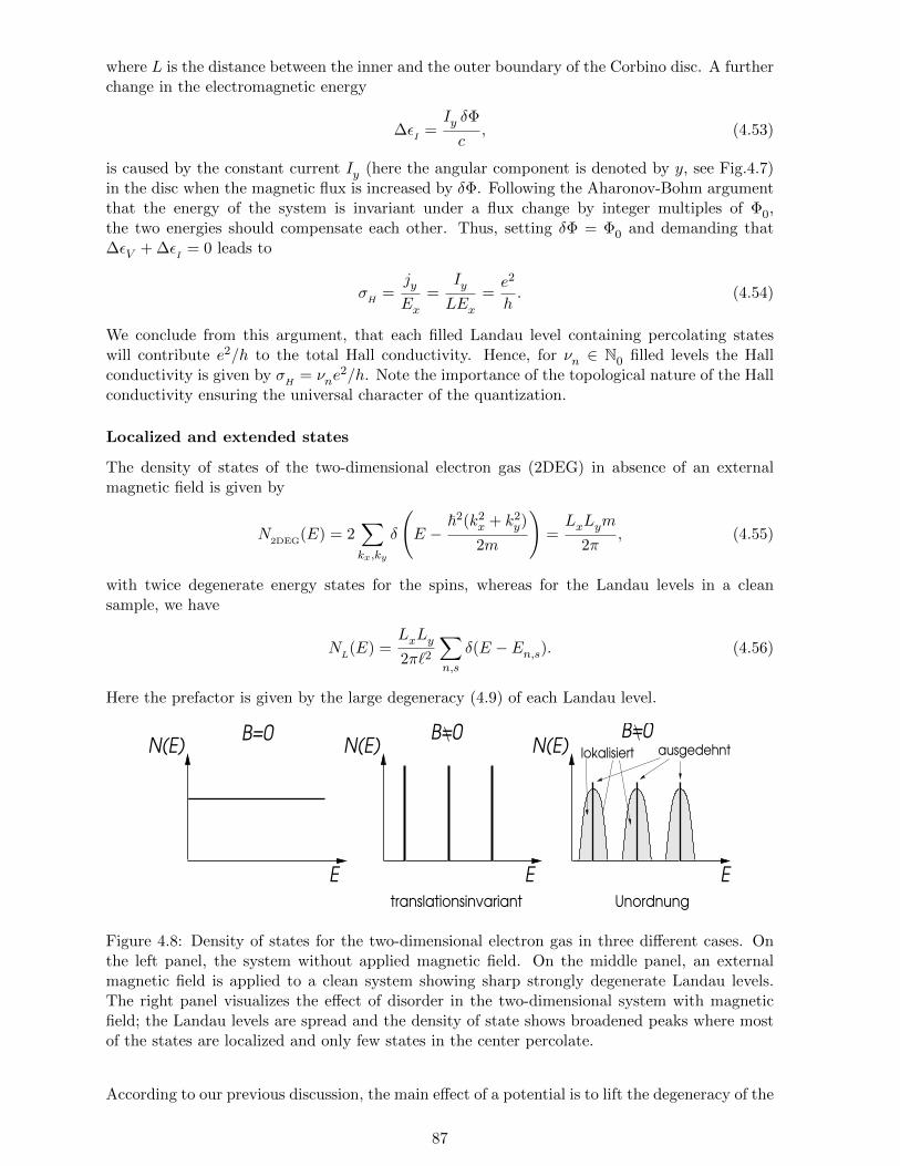
where L is the distance between the inner and the outer boundary of the Corbino disc. A furtherchange in the electromagnetic energy

∆εI

=Iy δΦ

c, (4.53)

is caused by the constant current Iy (here the angular component is denoted by y, see Fig.4.7)in the disc when the magnetic flux is increased by δΦ. Following the Aharonov-Bohm argumentthat the energy of the system is invariant under a flux change by integer multiples of Φ0,the two energies should compensate each other. Thus, setting δΦ = Φ0 and demanding that∆εV + ∆ε

I= 0 leads to

σH

=jyEx

=IyLEx

=e2

h. (4.54)

We conclude from this argument, that each filled Landau level containing percolating stateswill contribute e2/h to the total Hall conductivity. Hence, for νn ∈ N0 filled levels the Hallconductivity is given by σ

H= νne

2/h. Note the importance of the topological nature of the Hallconductivity ensuring the universal character of the quantization.

Localized and extended states

The density of states of the two-dimensional electron gas (2DEG) in absence of an externalmagnetic field is given by

N2DEG

(E) = 2∑kx,ky

δ

(E −

~2(k2x + k2

y)

2m

)=LxLym

2π, (4.55)

with twice degenerate energy states for the spins, whereas for the Landau levels in a cleansample, we have

NL(E) =

LxLy2π`2

∑n,s

δ(E − En,s). (4.56)

Here the prefactor is given by the large degeneracy (4.9) of each Landau level.

N(E) N(E)N(E)

E E E

translationsinvariant Unordnung

B=0lokalisiert ausgedehnt

B=0 B=0

Figure 4.8: Density of states for the two-dimensional electron gas in three different cases. Onthe left panel, the system without applied magnetic field. On the middle panel, an externalmagnetic field is applied to a clean system showing sharp strongly degenerate Landau levels.The right panel visualizes the effect of disorder in the two-dimensional system with magneticfield; the Landau levels are spread and the density of state shows broadened peaks where mostof the states are localized and only few states in the center percolate.

According to our previous discussion, the main effect of a potential is to lift the degeneracy of the

87

states comprising a Landau level. This remains true for random potential landscapes. Most ofthe states are then localized and do not contribute to electric transport. Only the few extendedstates contribute to the transport if they are filled (see Fig. 4.8). For partially filled extendedstates the Hall conductivity σ

His not an integer multiple of e2/h, since not all percolating states

– necessary for transferring one electron from one edge to the other, when the flux is changedby Φ0 (in Laughlin’s argument) – are occupied. Thus, the charge transferred does not amountto a complete −e. The appearance of partially filled extended states marks the transition fromone plateau to the next and is accompanied by a finite longitudinal conductivity σyy. When allextended states of a Landau level are occupied, the contribution to the longitudinal transportstops, i.e., in the range of a plateau σyy vanishes. Because of thermal occupation, the plateausquickly shrink when the temperature of the system is increased. This is the reason why theQuantum Hall Effect is only observable for sufficiently low temperatures (T < 4K).

Edge states and Buttiker’s argument

A confining potential prevents the electrons from leaving the metal. This potential at the edgesof the sample has also to be considered in the potential landscape. Interestingly, equi-potentialtrajectories of states close to the edge are always extended and percolate along the edge. Thecorresponding wave functions have already been discussed in Section 4.2.1. From Eq.(4.37), wefind that the energy is not symmetric in ky, the wave vector along the edge, i.e. E(ky) 6= E(−ky).This implies that the states are chiral and can move in one direction only for a given energy.The edge states on the opposing edges move in opposite directions, a fact that can be readilyverified by inspection of (4.37) based on Fig.4.9. The total current flowing along the edge for agiven Landau level is

I =∑ky

e

Lyvy, (4.57)

meaning that one state per ky extends over the whole length Ly of the Hall element. Thus,the density is given by 1/Ly. The wave vector is quantized according to the periodic boundaryconditions; ky = 2πny/Ly with ny ∈ Z. The velocity vy is given by equation (4.38). In summary,we have

I =e

2π~

∫occupied

dkydEn(ky)

dky=e

h

∫occupied

dx0

dE

dx0

=e

h(µ− E(0)

n ) (4.58)

where x0 = ky`2 is the transversal position of the wave function and µ is the chemical potential.

Sufficiently far away from the boundary En is independent of x0 and approaches the valueE(0)n = ~ωc(1/2+n) of a translationally invariant electron gas. The potential difference between

the two opposing edges leads to a net current along the edge direction of the Hall bar,

µA− µ

B= eV

H= eExLx =

h

e(IA

+ IB

) =h

eIH, (4.59)

and with that

σH

=IH

ExLx=e2

h, (4.60)

where for µA

= µB

we have IA

= −IB

. Note that IH

= IA

+ IB

is only valid when no currentsare present in the bulk of the system. The latter condition is ensured by the localization of thestates at the chemical potential. This argument by Buttiker leads to the same quantization asderived before, namely every Landau level contributes one edge state and thus σ

H= νne

2/h (νnis the number of occupied Landau levels). Note that this argument is independent of the precise

88

IA

IB

µ

E

x

µAµ

B

E

x

AB

L

x

E

µ

n=2

n=1

n=0

Figure 4.9: Edge state picture by Buttiker. The left panel gives a top view of the two dimensionalsystem (L = Lx) where chiral edge states exist on both edges of the Hall bar with oppositechirality. On the middle panel, a single Landau level without and with transverse potentialdifference is shown, where the latter yields a finite net current due to current imbalance betweenleft and right edge. The right panel visualizes the two lowest Landau levels which are occupied.All higher Landau levels are empty. This fixes the Hall conductance value νn to 2.

shape of the confining edge potential.Within this argument we are able to understand why the longitudinal conductivity has to vanishat the Hall plateaus. For that we express Ohm’s law However it is simpler to discuss theresistivity. Like the conductivity σ the resistivity ρ is a tensor:

j = σE (4.61)

E = ρj (4.62)

where the conductivity σ and the resistivity ρ are both a symmetric 2× 2 tensor with σxx = σyyand ρxx = ρyy. Therefore we find

σyy =ρyy

ρ2yy + ρ2

xy

, (4.63)

σxy =ρxy

ρ2yy + ρ2

xy

. (4.64)

In the following argument, we explain why the longitudinal resistivity ρyy in two dimensionshas to vanish in the presence of a finite Hall resistivity ρxy. Since the edge state electrons witha given energy can only move in one direction, there is no backward scattering by obstacles aslong as the edges are far apart from each other. No scattering between the two edges impliesρyy = 0 and hence σyy = 0. A finite resistivity can only occur when extended states are presentin the bulk, such that the edge states on opposite edges are no longer spatially separated fromeach other.

4.2.3 Fractional Quantum Hall Effect

Only two years after the discovery of the Integer Quantum Hall Effect, Stormer, Tsui andGossard observed further series of plateaus of the Hall resistivity in a 2DEG realized with veryhigh quality MOSFET inversion layers at low temperatures. The most pronounced of theseplateaus is observed at a filling of ν = 1/3 (σxy = νe2/h). Later, an entire hierarchy of plateausat fractional values ν = νp,m = p/m with p,m ∈ N has been discovered,

νp,m ∈

1

3,

2

3,

2

5,

3

5,

3

7, . . .

. (4.65)

The emergence of these new plateaus is a clear evidence of the so-called Fractional QuantumHall Effect (FQHE).

89

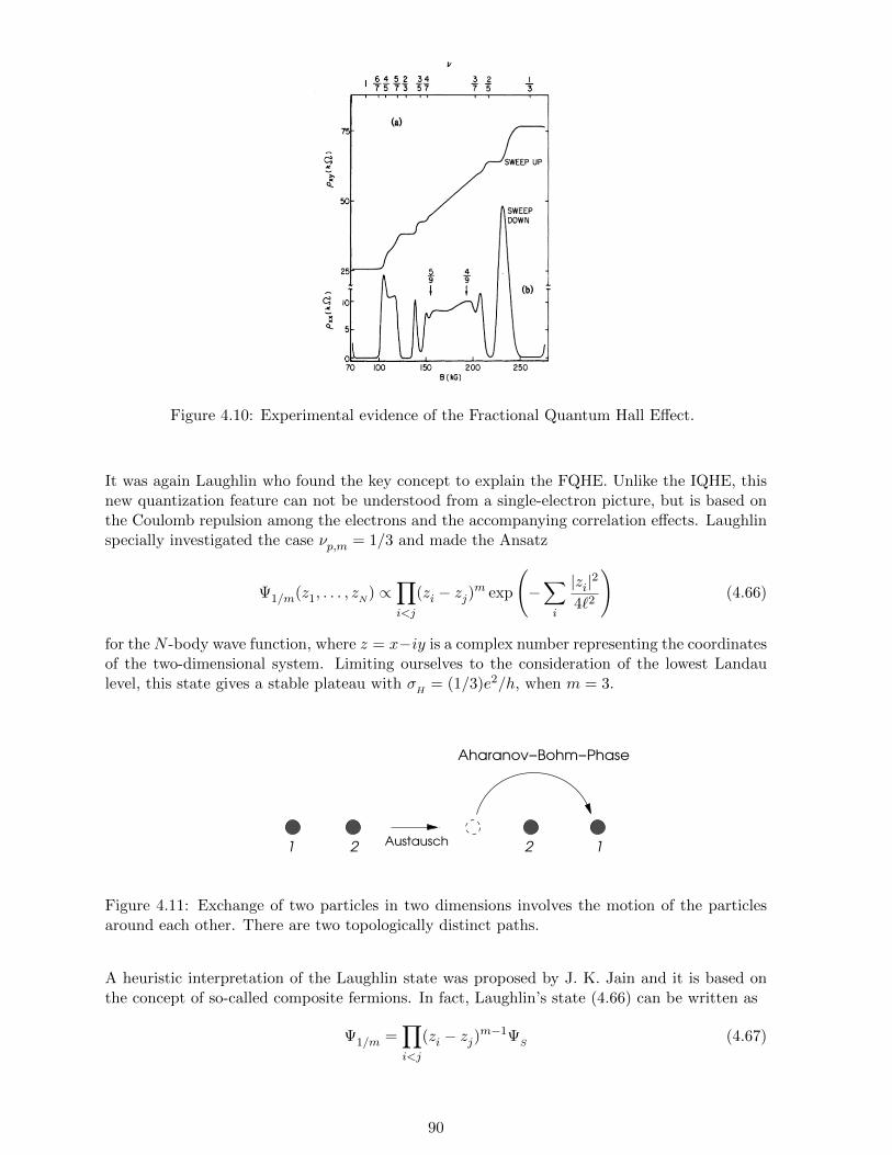
Figure 4.10: Experimental evidence of the Fractional Quantum Hall Effect.

It was again Laughlin who found the key concept to explain the FQHE. Unlike the IQHE, thisnew quantization feature can not be understood from a single-electron picture, but is based onthe Coulomb repulsion among the electrons and the accompanying correlation effects. Laughlinspecially investigated the case νp,m = 1/3 and made the Ansatz

Ψ1/m(z1, . . . , zN) ∝∏i<j

(zi − zj)m exp

(−∑i

|zi|24`2

)(4.66)

for the N -body wave function, where z = x−iy is a complex number representing the coordinatesof the two-dimensional system. Limiting ourselves to the consideration of the lowest Landaulevel, this state gives a stable plateau with σ

H= (1/3)e2/h, when m = 3.

121 2

Aharanov−Bohm−Phase

Austausch

Figure 4.11: Exchange of two particles in two dimensions involves the motion of the particlesaround each other. There are two topologically distinct paths.

A heuristic interpretation of the Laughlin state was proposed by J. K. Jain and it is based onthe concept of so-called composite fermions. In fact, Laughlin’s state (4.66) can be written as

Ψ1/m =∏i<j

(zi − zj)m−1ΨS

(4.67)

90

where ΨS

is the Slater determinant6 describing the completely filled lowest Landau level. Wesee that the prefactor of Ψ

Sin equation (4.67) acts as a so-called Jastrow factor that introduces

correlation effects into the wave function, since only the correlations due to the Pauli exclusionprinciple are contained in Ψ

S. The Jastrow factor treats the Coulomb repulsion among the

electrons and consequently leads to an additional suppression of the wave function whenevertwo electrons approach each other. In the form introduced above, it produces an phase factorfor the electrons encircling each other. In particular, exchanging two electrons (see Fig. 4.11)leads to a phase

exp(i(m− 1)π) = exp

(ie

~cm− 1

2Φ0

), (4.72)

since Φ0 = 2π~c/e. This phase has to be unity since the Slater state ΨS

is odd under exchangeof two electrons. Therefore m is restricted to odd integer values. This guarantees that the totalwave function Ψ1/m still changes sign when two electrons are exchanged.

−2Φ00

n0

+

composite

Fermioncomposite Fermion s

im externen Feld

Feld−Kompensation

IQHE

0 effB = B −

Beff

Bex

ex 2Φ

Figure 4.12: Sketch of the composite Fermion concept. Electrons with attached magnetic fluxlines, here for the state of ν = 1/3.

According to the Footnote 5 (see equation (4.39)), the case νp,m = 1/3 implies that there arethree flux quanta Φ0 per electron. In order to understand the FQHE, one constructs so-calledcomposite fermions which do not interact with each other. Here, a composite fermion consists of

6The Slater determinant of the lowest Landau level is obtained from the states of the independent electrons.In symmetric gauge, the states are labelled by the quantum number m ∈ N0 and apart from the normalization(given in equation (4.42)) they are given by

φm(z) = zme−|z|2/4`2 , (4.68)

where z = x− iy. The Slater determinant for N independent electrons is

ΨS(z1, . . . , zN) =1√N !

det

φ0(z1) · · · φN−1(z1)...

...φ0(zN) · · · φN−1(zN)

(4.69)

=1√N !

det

1 z1 z2

1 · · · zN−11

1 z2 z22 · · · zN−1

2

......

......

1 zN z2N · · · zN−1

N

exp

(−∑i

|zi|2

4`2

). (4.70)

The remaining determinant is a so-called Vandermonde determinant, which can be reexpressed in the form of aproduct, such that

ΨS =∏i<j

(zi − zj) exp

(−∑i

|zi|2

4`2

). (4.71)

The prefactor is a homogenous polynomial with roots whenever zi = zj , which is a manifestation of the Pauliexclusion principle. We also see that the state ΨS has a well defined total angular momentum Lz = N~.

91

an electron that has two (in fact m− 1) negative flux quanta attached to it. These objects maybe considered as independent fermions since the attached flux quanta compensate the Jastrowfactor in equation 4.67 through factors of the type (zi − zj)−(m−1). The exchange of two suchcomposite fermions in two dimensions leads to an Aharanov-Bohm phase that is just opposedto that in equation (4.72). Due to the presence of the flux −2Φ0 per electron, the compositefermions are subject to an effective field composed of the external field and the attached fluxquanta:

Beff = B −∑i

2Φ0(zi) (4.73)

=1

3B −

(∑i

2Φ0(zi)−2

3B

)(4.74)

For an external field B = 3n0Φ0, the expression in the brackets of equation (4.74) vanishes andthe composite fermions feel an effective field Beff = n0Φ0 (Fig. (4.12)). Thus, these fermionsform an Integer Quantum Hall state with ν = 1 (for B = 3n0Φ0), as discussed previously. Thisway of interpretation is applicable to other Fractional Quantum Hall states, too, since for nfilled Landau levels with composite fermions consisting of an electron with an attached flux of−2kΦ0, the effective field reads

Beff = n0

Φ0

νp,m− 2kn0Φ0 = n0

Φ0

n. (4.75)

From this we infer, that

1

n+ 2k =

1

νp,m(4.76)

or equivalently

νp,m =p

m=

n

2kn+ 1. (4.77)

Despite the apparent simplicity of the treatment in terms of independent composite fermions, oneshould keep in mind that one is dealing with a strongly correlated electron system. The structureof the composite fermions is a manifestation of the fact that the fermions are not independentelectrons. No composite fermions can exist in the vacuum, they can only arise within a certainmany-body state. The Fractional Quantum Hall state also exhibits unconventional excitationswith fractional charges. For example in the case νp,m = 1/3, there are excitations with effectivecharge e∗ = e/3. These are so-called ’topological’ excitations, that can only exist in correlatedsystems. The Fractional Quantum Hall system is a very peculiar ’ordered’ state of a two-dimensional electron system that has many interesting and complex properties.7

7Additional literature on the quantum Hall effects. For the Integer quantum Hall effect consult

- K. von Klitzing et al., Physik Journal 4 (6), 37 (2005)

while detailed literature on the fractional quantum Hall effect is found in

- R. Morf, Physik in unserer Zeit 33, 21 (2002)

- J.K. Jain, Advances in Physics 41, 105 (1992).

92

Chapter 5

Landau’s Theory of Fermi Liquids

In the previous chapters, we considered the electrons of the system as more or less independentparticles. The effect of their mutual interactions only entered via the renormalization of poten-tials and collective excitations. The underlying assumptions of our earlier discussions were thatelectrons in the presence of interactions can still be described as particles with a well-definedenergy-momentum relation, and that their groundstate is a filled Fermi sea with a sharp Fermisurface. Since there is no guarantee that this hypothesis holds in general (and in fact they donot), we have to show that in metals the description of electrons as quasiparticles is justified.This quasiparticle picture will lead us to Landau’s phenomenological theory of Fermi liquids.

5.1 Lifetime of quasiparticles

We first consider the lifetime of a state consisting of a filled Fermi sea to which one electronis added. Let k with |k| > k

F(εk = ~2k2/2m with εk > ε

F) be the momentum (energy) of

the additional electron. Due to interactions between the electrons, this state will decay into amany-body state. In momentum space such an interaction takes the form

Hee =∑k,k′,q

∑s,s′

V (q)c†k−q,sc†k′+q,s′

ck′,s′ ck,s, (5.1)

where V (q) represents the electron-electron interaction in momentum space while q indicatesthe momentum transfer in the scattering process. Below, the short-ranged Yukawa potential

V (q) =4πe2

q2ε(q, 0)=

4πe2

q2 + k2TF

(5.2)

from equation (3.94) will be used. As we are only interested in very small energy transfers~ω ε

F, the static approximation is admissible.

k’

k

k−qk’+q

Figure 5.1: The decay of an electron state above the Fermi energy happens through scatteringby creating particle-hole excitations.

In a perturbative treatment, the lowest order effect of the interaction is the creation of a particle-hole excitation in addition to the single electron above the Fermi energy. As the additional

93

electron changes its momentum from k to k−q, a hole appears at k′ and a second electron withwavevector k′ + q is created outside the Fermi sea. The transition is allowed whenever bothenergy and momentum are conserved, meaning

k = (k − q)− k′ + (k′ + q), (5.3)

and

εk = εk−q − εk′ + εk′+q. (5.4)

We calculate the lifetime τk of the initial state with momentum k using Fermi’s golden rule,yielding the transition rate from the initial state of a filled Fermi sea and one particle withmomentum k to a state with two electrons above the Fermi sea, with momenta k−q and k′+q,and a hole with k′, as shown in Fig. 5.1. Since neither the momenta k′ and q, nor the spin ofthe created electron are fixed, a summation over the possible configuration has to be performed,leading to

1

τk=

2π

~1

Ω2

∑k′,q

∑s′

|V (q)|2 n0,k′(1− n0,k−q)(1− n0,k′+q)δ(εk−q − εk − (εk′ − εk′+q)). (5.5)

Note that the term n0,k′(1− n0,k−q)(1− n0,k′+q) takes care of the Pauli principle, by ensuring

that the final state after the scattering process exists, i.e. the hole state k′ lies inside and thetwo particle states k − q and k′ + q lie outside the Fermi sea. First the integral over k′ isperformed under the condition that the energy εk′+q − εk′ of the excitation is small. With that,the integral reduces to

S(ωq,k, q) =1

Ω

∑k′

n0,k′(1− n0,k′+q)δ(εk−q − εk − (εk′ − εk′+q)) (5.6)

=1

(2π)3

∫d3k′ n0,k′(1− n0,k′+q)δ(εk′+q − εk′ − ~ωq,k) (5.7)

=N(ε

F)

4

ωq,kqvF

(5.8)

where N(εF

) = mkF/π2~2 is the density of states of the electrons at the Fermi surface and

~ωq,k = ~2(2k ·q−q2)/2m > 0 is the energy loss of the decaying electron.1 In order to compute

1Small ω are justified, because ~ω ≤ (2kF q− q2)/2m for most allowed ω. The integral may be computed usingcylindrical coordinates, where the vector q points along the axis of the cylinder. It results in

S(q, ω) =1

(2π)2

k1∫k2

dk′⊥k′⊥

kF∫0

dk′‖ δ

(~2q2

2m+

~2qk′‖m

− ~ω

)(5.9)

=m

4π2~2q

(k2

1 − k22

), (5.10)

with k21 = k2

F − k2‖,0 and k2

2 = k2F − (k‖,0 + q)2, where k‖,0 = (2mω − ~q2)/2~q is enforced by the delta function.

q

||

kF

kF

k2

k1

k

The wave vectors k2 and k1 are the upper and lower limits of integration determined from the condition n0,k′(1−n0,k′+q) > 0 and can be obtained by simple geometric considerations. equation (5.8) follows immediately.

94

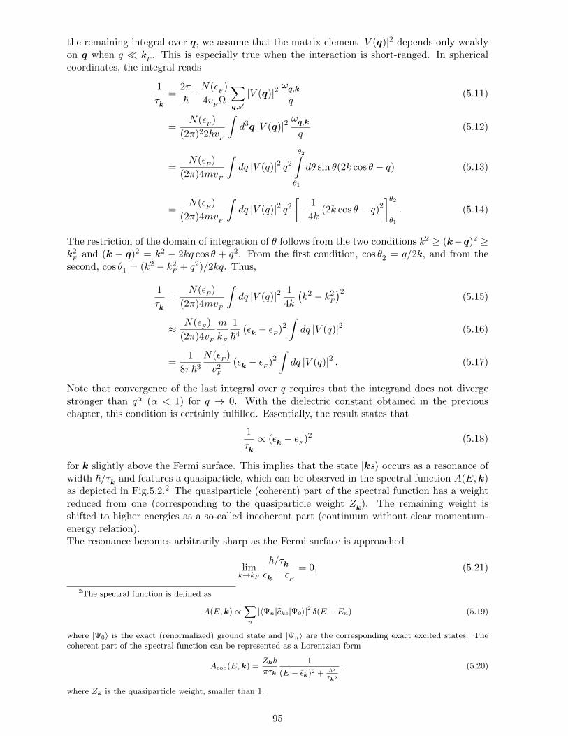
the remaining integral over q, we assume that the matrix element |V (q)|2 depends only weaklyon q when q k

F. This is especially true when the interaction is short-ranged. In spherical

coordinates, the integral reads

1

τk=

2π

~· N(ε

F)

4vF

Ω

∑q,s′

|V (q)|2ωq,kq

(5.11)

=N(ε

F)

(2π)22~vF

∫d3q |V (q)|2

ωq,kq

(5.12)

=N(ε

F)

(2π)4mvF

∫dq |V (q)|2 q2

θ2∫θ1

dθ sin θ(2k cos θ − q) (5.13)

=N(ε

F)

(2π)4mvF

∫dq |V (q)|2 q2

[− 1

4k(2k cos θ − q)2

]θ2θ1

. (5.14)

The restriction of the domain of integration of θ follows from the two conditions k2 ≥ (k−q)2 ≥k2F

and (k − q)2 = k2 − 2kq cos θ + q2. From the first condition, cos θ2 = q/2k, and from thesecond, cos θ1 = (k2 − k2

F+ q2)/2kq. Thus,

1

τk=

N(εF

)

(2π)4mvF

∫dq |V (q)|2 1

4k

(k2 − k2

F

)2(5.15)

≈ N(εF

)

(2π)4vF

m

kF

1

~4(εk − εF )2

∫dq |V (q)|2 (5.16)

=1

8π~3

N(εF

)

v2F

(εk − εF )2∫dq |V (q)|2 . (5.17)

Note that convergence of the last integral over q requires that the integrand does not divergestronger than qα (α < 1) for q → 0. With the dielectric constant obtained in the previouschapter, this condition is certainly fulfilled. Essentially, the result states that

1

τk∝ (εk − εF )2 (5.18)

for k slightly above the Fermi surface. This implies that the state |ks〉 occurs as a resonance ofwidth ~/τk and features a quasiparticle, which can be observed in the spectral function A(E,k)as depicted in Fig.5.2.2 The quasiparticle (coherent) part of the spectral function has a weightreduced from one (corresponding to the quasiparticle weight Zk). The remaining weight isshifted to higher energies as a so-called incoherent part (continuum without clear momentum-energy relation).The resonance becomes arbitrarily sharp as the Fermi surface is approached

limk→kF

~/τkεk − εF

= 0, (5.21)

2The spectral function is defined as

A(E,k) ∝∑n

|〈Ψn|cks|Ψ0〉|2 δ(E − En) (5.19)

where |Ψ0〉 is the exact (renormalized) ground state and |Ψn〉 are the corresponding exact excited states. Thecoherent part of the spectral function can be represented as a Lorentzian form

Acoh(E,k) =Zk~πτk

1

(E − εk)2 + ~2τk2

, (5.20)

where Zk is the quasiparticle weight, smaller than 1.

95

incoherent part

FE

F E

kA(E,k)

Quasiparticle

k

Figure 5.2: Quasiparticle spectrum: Quasiparticle peaks appear the sharper the closer theenergy lies to the Fermi energy. The area under the “sharp” quasiparticle peak corresponds tothe quasiparticle weight. The missing quasiparticle weight is transferred to higher energies.

so that the quasiparticle concept is asymptotically valid. The equation (5.21) can also be seen asa verification of Heisenberg’s uncertainty principle. Consequently, the momentum of an electronis a good quantum number in the vicinity of the Fermi surface. Underlying this result is thePauli exclusion principle, which restricts the phase space for decay processes of single particlestates close to the Fermi surface. In addition, the assumption of short ranged interactions iscrucial. Long ranged interactions can change the behavior drastically due to the larger numberof decay channels.

5.2 Phenomenological Theory of Fermi Liquids

The existence of well-defined fermionic quasiparticles in spite of the underlying complex many-body physics inspired Landau to the following phenomenological theory. Just like the states ofindependent electrons, quasiparticle states shall be characterized by their momentum k and spinσ. In fact, there is a one-to-one mapping between the free electrons and the quasiparticles. Con-sequently, the number of quasiparticles and the number of electrons coincide. The momentumdistribution function of quasiparticles, defined as nσ(k), is subject to the condition

N =∑k,σ

nσ(k). (5.22)

In analogy to the Fermi-Dirac distribution of free electrons, one demands, that the ground statedistribution function n(0)

σ (k) for the quasiparticles is described by a simple step function

n(0)σ (k) = Θ(k

F− |k|). (5.23)

For a spherically symmetric electron system, the quasiparticle Fermi surface is a sphere withthe same radius as the one for free electrons of the same density. For a general point groupsymmetry, the Fermi surface may be deformed by the interactions without changing the un-derlying symmetry. The volume enclosed by the Fermi surface is always conserved despite thedeformation.3 Note that the distribution n(0)

σ (k) of the quasiparticles in the ground state and

that n0ks = 〈c†kσ ckσ〉 of the real electrons in the ground state are not identical (Figure 5.3).Interestingly, n0ks is still discontinuous at the Fermi surface, but the height of the jump is, ingeneral, smaller than unity. The modification of the electron distribution function from a step

3This is the content of the Luttinger theorem [J.M. Luttinger, Phys. Rev. 119, 1153 (1960)].

96

kFk

F

n0ks

n (k)

kk

σ

Figure 5.3: Schematic picture of the distribution function: Left panel: modified distributionfunction of the original electron states; right panel: distribution function of quasiparticle statesmaking a simple step function.

function to a “smoother” Fermi surface indicates the involvement of electron-hole excitationsand the renormalization of the electronic properties, which deplete the Fermi sea and populatethe states above the Fermi level. The reduced jump in n0ks is a measure for the quasiparticleweight at the Fermi surface, ZkF , i.e. the amplitude of the corresponding free electron state inthe quasiparticle state.In Landau’s theory of Fermi liquids, the essential information on the low-energy physics of thesystem shall be contained in the deviation of the quasiparticle distribution nσ(k) from its groundstate distribution n(0)

σ (k),

δnσ(k) = nσ(k)− n(0)σ (k). (5.24)

The symbol δ is generally used in literature to denote this difference. Unfortunately this maysuggest that the term δnσ(k) is small, which is not true in general. Indeed, δnσ(k) is con-centrated on momenta k very close to the Fermi energy only, where the quasiparticle conceptis valid. This distribution function, describing the deviation from the ground state, enters aphenomenological energy functional of the form

E = E0 +∑k,σ

εσ(k)δnσ(k) +1

2Ω

∑k,k′

∑σ,σ′

fσσ′(k,k′)δnσ(k)δnσ′(k

′) +O(δn3) (5.25)

where E0 denotes the energy of the ground state. Moreover, the phenomenological parametersεσ(k) and fσσ′(k,k

′) have to be determined by experiments or by means of a microscopic theory.The variational derivative

εσ(k) =δE

δnσ(k)= εσ(k) +

1

Ω

∑k′,σ′

fσσ′(k,k′)δnσ′(k

′) (5.26)

yields an effective energy-momentum relation εσ(k), whose second term depends on the distribu-tion of all quasiparticles. A quasiparticle moves in the “mean-field” of all other quasiparticles, sothat changes δnσ(k) in the distribution affect εσ(k). The second variational derivative describesthe coupling between the quasiparticles

δ2E

δnσ(k)δnσ′(k′)

=1

Ωfσσ′(k,k

′). (5.27)

We introduce a parametrization for these couplings fσσ′(k,k′) by assuming spherical symmetry

of the system. Furthermore, the radial dependence is ignored, as we only consider quasiparticlesin the vicinity of the Fermi surface where |k|, |k′| ≈ k

F. Therefore the dependence of fσσ′(k,k

′)on k,k′ can be reduced to the relative angle θk,k′

fσσ′(k,k′) = fs(k, k′) + σσ′fa(k, k′) (5.28)

97

where k = k/|k|. The symmetric (s) and antisymmetric (a) part of fσσ′(k,k′) can be expanded

in Legendre-polynomials Pl(z)4, leading to

fs,a(k, k′) =∞∑l=0

fs,al Pl(cos θk,k′). (5.31)

The density of states at the Fermi surface is defined as

N(εF

) =2

Ω

∑k

δ(ε(k)− εF

) =k2F

π2~vF=m∗k

F

π2~2(5.32)

and follows from the dispersion ε(k) of the bare quasiparticle energy

∇k ε(k)|kF = vF =~k

F

m∗(5.33)

where for a fully rotation symmetric system we may write ε(k) = ~2k2/2m∗ with m∗ as an”effective mass”, although we will be only interested at the spectrum in the immediate vicinityof the Fermi energy. With this definition, we also introduce the so-called Landau parameters

F sl = N(εF

)fsl , (5.34)

F al = N(εF

)fal , (5.35)

commonly used in the literature.5 In the following, we want to study the relation between the dif-ferent phenomenological parameters of Landau’s theory of Fermi liquids and the experimentallyaccessible quantities of a real system, such as specific heat, compressibility, spin susceptibilityamong others.

5.2.1 Specific heat - Density of states

Since the quasiparticles are fermions, they obey Fermi-Dirac statistics

n(0)σ (T,k) =

1

e[ε(k)−µ]/kBT + 1(5.36)

with the chemical potential µ. For low temperatures, we find

δnσ(k) = n(0)σ (T,k)− n(0)

σ (0,k) (5.37)

which, using Eq.(5.26) leads to ε(k) = ε(k), because here

1

Ω

∑k′,σ′

fσσ′(k,k′)δnσ′(k

′) = 0 . (5.38)

In δnσ′(k′) there are as many particles (positive) as holes (negative) such that they cancel in

the correction term. Therefore we rewrite the Fermi-Dirac distribution (5.36) as

nσ(k) =1

e[ε(k)−εF ]/kBT + 1(5.39)

4Legendre-Polynomials: The Legendre polynomials satisfy the orthogonality relation∫dΩk4π

Pl(cos θk)Pl′(cos θk) =

∫ +1

−1

dzPl(z)Pl′(z) =2δll′

2l + 1(5.29)

for all l = 0, 1, 2, .... The first few polynomials are

P0(z) = 1 , P1(z) = z , P2(z) =1

2(3z2 − 1) , P3(z) =

1

2(5z3 − 3z) . (5.30)

5Another frequently used notation for the Landau parameters in the literature is Fl = F sl and Zl = F al .

98

with the bare quasiparticle energy εσ(k) in place of the renormalized dispersion εσ(k). Further-more, we replaced µ = ε

F+ O(T 2) by ε

F. When focussing on leading terms, which are usually

of the order T 0 and T 1, corrections of higher order may be neglected in the low-temperatureregime. In order to discuss the specific heat, we employ the expression for the entropy of afermion gas. For each quasiparticles with a given spin there is one state labelled by k. Theentropy density may be computed from the distribution function

S = −kBΩ

∑k,σ

[nσ(k) ln (nσ(k)) + (1− nσ(k)) ln (1− nσ(k))

]. (5.40)

Taking the derivative of the entropy S with respect to T , the specific heat

C(T ) = T∂S

∂T(5.41)

= −kBTΩ

∑k,σ

eξ(k)/kBT

( eξ(k)/kBT + 1 )2

ξ(k)

kBT 2

ln

(nσ(k)

1− nσ(k)

)(5.42)

= −kBTΩ

∑k,σ

1

4 cosh (ξ(k)/2kBT )2

ξ(k)

kBT 2

ξ(k)

kBT

(5.43)

is obtained, where we introduced ξ(k) = ε(k)− εF

. In the limit T → 0 we find

C(T )

T≈ N(ε

F)

4kBT 3

∫dξ

ξ2

cosh2(ξ/2kBT )

(5.44)

≈ k2BN(ε

F)

4

+∞∫−∞

dyy2

cosh2(y/2)(5.45)

=π2k2

BN(ε

F)

3, (5.46)

which is the well-known linear behavior C(T ) = γT for the specific heat at low temperatures,with γ = π2k2

BN(ε

F)/3. Since N(ε

F) = m∗k

F/π2~2, the effective mass m∗ of the quasiparticles

can directly determined by measuring the specific heat of the system.

5.2.2 Compressibility - Landau parameter Fs0

A Fermi gas has a finite compressibility because each fermion occupies a finite amount of spacedue to the Pauli principle. The compressibility κ is defined as6

κ = − 1

Ω

(∂Ω

∂p

)T,N

(5.48)

where p is the uniform hydrostatic pressure. The indices T,N mean, that the temperature Tand the particle number N are kept fixed. We consider the response of the Fermi liquid uponapplication of uniform pressure p. The shift of the quasiparticle energies is given by

δε(k) =∂ε(k)

∂pδp =

∂ε(k)

∂k· ∂k∂Ω

∂Ω

∂pδp =

κ(0)

3~vk · k δp = γkκ

(0)δp (5.49)

6An alternative definition considers the change of particle number upon change of the chemical potential,

κ =1

n2

(∂n

∂µ

)T,Ω

(5.47)

with n = N/Ω.

99

with γk = ~vk · k/3 = 2εσ(k)/3. Analogous we introduce the shift of the renormalized quasi-particle energies,

δεσ(k) = γkκδp = γkκ(0)δp+

1

Ω

∑k′,σ′

fσ,σ′(k,k′)δnσ′(k

′)

= γkκ(0)δp+

1

Ω

∑k′,σ′

fσ,σ′(k,k′)∂nσ′(k

′)∂εσ′(k

′)δεσ′(k

′)

= γkκ(0)δp− 1

Ω

∑k′,σ′

fσ,σ′(k,k′)δ(εσ′(k

′)− εF )γk′κ δp

. (5.50)

Changes are concentrated on the Fermi surface such that we can replace γk = 2εF /3 so that

κ = κ(0) − κN(εF )

∫dΩk′

4πf s(k, k′) = κ(0) − κF s0 . (5.51)

Therefore we find

κ =κ(0)

1 + F s0. (5.52)

Now we determine κ(0) from the volume dependence of the energy

E(0) =∑k,σ

εσ(k) =3

5NεF =

3

5N

~2k2F

2m∗=

3

10

~2N

m∗

(3π2N

Ω

)2/3

. (5.53)

Then we determine the pressure

p = −(∂E(0)

∂Ω

)N

=1

5

~2N

m∗

(3π2N

Ω

)2/3 1

Ω(5.54)

and1

κ(0)= −Ω

∂p

∂Ω=

1

3

~2N

m∗Ω(3π2n)2/3 =

2

3nεF . (5.55)

kF

kδk kδF Fδ

F

kF

Figure 5.4: Deviations of the distribution functions: Left panel: isotropic increase of the Fermisurface as used for the uniform compressibility; right panel: spin dependent change of size ofthe Fermi surface as used for the uniform spin susceptibility.

100

5.2.3 Spin susceptibility - Landau parameter Fa0

In a magnetic field H coupling to the electron spins the bare quasiparticle energy is supplementedby the Zeeman term,

εσ(k) =~2k2

2m∗− gµBH

σ

2(5.56)

where σ = ±1 denotes the spin component parallel to the applied field. The shift of therenormalized quasiparticle energy due to the applied field is

δεσ(k) = εσ(H,k)− ε(H = 0,k)

= −gµBHσ

2+

1

Ω

∑k′,σ′

fσ,σ′(k,k′)δnσ′(k

′) (5.57)

= −gµBHσ

2.

Note that by symmetry, δnσ(k) = −δn−σ(−k). Due to interactions, the renormalized gyromag-netic factor g differs from the value of g = 2 for free electrons. We focus on the second term inEq.(5.57), which can be reexpressed as

1

Ω

∑k′,σ′

fσσ′(k,k′)δnσ′(k

′) =1

Ω

∑k′,σ′

fσσ′(k,k′)∂nσ′(k

′)∂εσ′(k

′)δεσ′(k

′)

=1

Ω

∑k′,σ′

fσσ′(k,k′)δ(εσ′(k

′)− εF

)gµBHσ′

2(5.58)

Combining this result with the Eqs. (5.57) and (5.58), we derive

g = g − gN(εF

)

∫dΩk′

4πfa(k, k′) = g − gF a0 , (5.59)

or equivalently

g =g

1 + F a0. (5.60)

The magnetization of the system can be computed from the distribution function,

M = gµB

∑k,σ

σ

2δnσ(k) = gµ

B

∑k,σ

σ

2

∂nσ(k)

∂εσ(k)δεσ(k)

= gµB

∑k,σ

σ

2δ(εσ(k)− ε

F)gµ

BHσ

2(5.61)

from which the susceptibility is immediately found to be

χ =M

HΩ=µ2BN(ε

F)

1 + F a0. (5.62)

The changes in the distribution function induced by the magnetic field feed back into the sus-ceptibility, so that the latter may be either weakened (F a0 > 0) or enhanced (F a0 < 0). For themagnetic susceptibility, the Landau parameter F a0 and the effective mass m∗ (through N(ε

F))

lead to a renormalization compared to the free electron susceptibility.

101

5.2.4 Galilei invariance - effective mass and Fs1

We initially introduced by hand the effective mass of quasiparticles in εσ(k). In this sectionwe show, that overall consistency of the phenomenological theory requires a relation betweenthe effective mass and one Landau parameter (F s1 ). The reason is, that the effective massis the result of the interactions among the electrons. This self-consistency is connected withthe Galilean invariance of the system. When the momenta of all particles are shifted by ~q(|q| shall be very small compared to the Fermi momentum k

Fin order to remain within the

assumption-range of the Fermi liquid theory) the distribution function given by

δnσ(k) = n(0)σ (k + q)− n(0)

σ (k) ≈ q ·∇k n(0)σ (k). (5.63)

This function is strongly concentrated around the Fermi energy (see Figure 5.5).

n=−1δ n=+1δ

F qk

Figure 5.5: Distribution function due to a Fermi surface shift (Galilei transformation).

The current density can now be calculated, using the distribution function nσ(k) = n(0)σ (k) +

δnσ(k). Within the Fermi liquid theory this yields,

jq =1

Ω

∑k,σ

v(k)nσ(k) =1

Ω

∑k,σ

v(k)δnσ(k) (5.64)

with

v(k) =1

~∇k εσ(k)

=1

~

(∇k εσ(k) +

1

Ω

∑k′,σ′

∇k fσσ′(k,k′)δnσ(k′)). (5.65)

Thus we obtain for the current density,

jq =1

Ω

∑k,σ

~km∗

nσ(k) +1

Ω2

∑k,σ

∑k′,σ′

[n(0)σ (k) + δnσ(k)]

1

~∇k fσσ′(k,k′)δnσ(k′)

=1

Ω

∑k,σ

~km∗

δnσ(k)− 1

Ω2

∑k,σ

∑k′,σ′

1

~[∇k n(0)

σ (k)]fσσ′(k,k′)δnσ(k′) +O(q2) (5.66)

=1

Ω

∑k,σ

~km∗

δnσ(k) +1

Ω2

∑k,σ

∑k′,σ′

fσσ′(k,k′)δ(εσ(k′)− ε

F)~k′

m∗δnσ(k) +O(q2) = j1 + j2.

where, for the second line, we performed an integration by parts and neglect terms quadratic inδn and, in the third line, used fσσ′(k,k

′) = fσ′σ(k′,k) and

∇k n(0)σ (k) =

∂n(0)σ (k)

∂εσ(k)∇k εσ(k) = −δ(εσ(k)− ε

F)∇k εσ(k) = −δ(εσ(k)− ε

F)~2k

m∗. (5.67)

102

The first term of equation (5.67) denotes quasiparticle current, j1, while the second term canbe interpreted as a drag current, j2, an induced motion (backflow) of the other particles due tointeractions.

From a different viewpoint, we consider the system as being in the inertial frame with a velocity~q/m, as all particles received the same momentum. Here m is the bare electron mass. Thecurrent density is then given by

jq =N

Ω

~qm

=1

Ω

∑k,σ

~kmnσ(k) =

1

Ω

∑k,σ

~kmδnσ(k). (5.68)

Since these two viewpoints have to be equivalent, the resulting currents should be the same.Thus, we compare equation (5.67) and (5.68) and obtain the equation,

~km

=~km∗

+1

Ω

∑k′,σ′

fσσ′(k,k′)δ(εσ(k′)− ε

F)~k′

m∗(5.69)

which with k = k/kF then leads to

1

m=

1

m∗+N(ε

F)

∫dΩk′

4πfs(k, k′)

k · k′m∗

=1

m∗+

1

m∗

∫dΩk′

4πN(ε

F)fs(k, k′)︸ ︷︷ ︸∑∞

l=0 Fsl Pl(cos θk′ )

cos θk′︸ ︷︷ ︸P1(cos θk′ )

(5.70)

or by using the orthogonality of the Legendre polynomials,

m∗

m= 1 +

1

3F s1 . (5.71)

where 1/3 = 1/(2l + 1) for l = 1 originates from the orthogonality relation of Legendre-polynomials, as shown above. Therefore, the relation (5.71) has to couple m∗ to F s1 in order forLandau’s theory of Fermi liquids to be self-consistent. Generally, we find that F s1 > 0 so thatquasiparticles in a Fermi liquid are effectively heavier than bare electrons.

5.2.5 Stability of the Fermi liquid

Upon inspection of the renormalization of the quantities treated previously

γ

γ0

=m∗

m, (5.72)

κ

κ0

=m∗

m

1

1 + F s0, (5.73)

χ

χ0

=m∗

m

1

1 + F a0(5.74)

withm∗

m= 1 +

1

3F s1 , (5.75)

and the the response functions of the non-interacting system are given by

γ0 =k2BmkF3~2

, κ0 =3m

n~2k2F

and χ0 = µ2B

mkFπ2~2

(5.76)

one notes that the compressibility κ (susceptibility χ) diverges for F s0 → −1 (F a0 → −1),indicating an instability of the system. A diverging spin susceptibility for example leads to aferromagnetic state with a split Fermi surface, one for each spin direction. On the other hand, adiverging compressibility leads to a spontaneous contraction of the system. More generally, the

103

deformation of the quasiparticle distribution function may vary over the Fermi surface, so thatarbitrary deviations of the Fermi liquid ground state may be classified by the deformation

δnσ(k) =

∞∑l=0

+l∑m=−l

δnσ,l,mYlm(θk, φk) (5.77)

Note that we allow here formally for complex distribution functions. For pure charge density de-formations we have δn+,l,m(k) = δn−,l,m(k), while pure spin density deformations are described

by δn+,l,m(k) = −δn−,l,m(k). The general response function for a redistribution δnσ(k) with the

anisotropy Ylm(θk, φk) is given by 7

χl,m =χ

(0)l,m

1 +F s,al2l+1

. (5.85)

Stability of the Fermi liquid against any of these deformations requires

1 +F s,al

2l + 1> 0. (5.86)

If for any deformation channel l this conditions is violated one talks about a ”Pomeranchuckinstability”.8 Generally, the renormalization of the Fermi liquid leads to a change in the Wilsonratio, defined as

R

R0

=χ

χ0

γ0

γ=

1

1 + F a0(5.87)

7General response and distribution deformations: We consider a force field F with conjugate ”polarisation” Pwhich yields a modification of the quasiparticle dispersion,

δεσ(k) = −αλσ(k)F and δεσ(k) = −αλσ(k)F (5.78)

where we assume that λσ(k) = Yl,m(θk, φk) = (−1)mY ∗l,−m(θk, φk) without spin dependence. Then we can write

εσ(k) = δεσ(k) +1

Ω

∑k′,σ′

fσσ′(k, k′)δnσ′(k

′) = δεσ(k) +1

Ω

∑k′,σ′

fσσ′(k, k′)

∂nσ′

∂εσ′(k′)δεσ′(k

′) . (5.79)

In the last step we take for δnσ′(k′) the self-consistent value taking the feedback of the quasiparticle coupling

into account. We now use the relation

fs,a(k, k′) =

∞∑l=0

fs,al Pl(k · k′) = 4π

∞∑l=0

fs,al2l + 1

+l∑m=−l

Ylm(θk, φk)Y ∗lm(θk′ , φk′) (5.80)

and insert Eq.(5.78) to find

αλσ(k)F = αλσ(k)F −N(εF )fsl

2l + 1Ylm(θk, φk)α

∫dΩk′Y

∗lm(θk′ , φk′)λσ(k′)F (5.81)

which leads straightforwardly to

α = α− α F sl2l + 1

⇒ α =α

1 +Fsl

2l+1

. (5.82)

Now the polarisation is calculated which we may define as

P = − 1

Ω

∑k,σ

αλσ(k)δnσ(k) = − 1

Ω

∑k,σ

αλσ(k)∂nσ′

∂εσ(k)δεσ(k) = ααN(εF )F (5.83)

such that the linear response is given by

χ =P

F=α2N(εF )

1 +Fsl

2l+1

. (5.84)

8I.J. Pomeranchuk, JETP 8, 361 (1958)

104

where R0 = χ0/γ0 = 6µ2B/π2k2

B. Note that the Wilson ratio does not depend on the effective

mass. A remarkable feature of the Fermi liquid theory is that even very strongly interactingFermions remain Fermi liquids, notably the quantum liquid 3He and so-called heavy Fermionsystems, which are compounds of transition metals and rare earths. Both are strongly renormal-ized Fermi liquids. For 3He we give some of the parameters in Table 5.1 both for zero pressureand for pressures just below the critical pressure at which He solidifies (pc ≈ 2.5MPa = 25bar).

pressure m∗/m F s0 F a0 F s1 κ/κ0 χ/χ0

p = 0 3.0 10.1 -0.52 6.0 0.27 6.3

p < pc 6.2 94 -0.74 15.7 0.065 24

Table 5.1: List of the parameters of the Fermi liquid theory for 3He at zero pressure and at apressure just below solidification.

The trends show obviously, that the higher the applied pressure is, the denser the liquid becomesand the stronger the quasiparticles interact. Approaching the solidification the compressibilityis reduced, the quasiparticles become heavier (slower) and the magnetic response increases dras-tically. Finally the heavy fermion systems are characterized by the extraordinary enhancementsof the effective mass which for many of these compounds lie between 100 and 1000 times higherthan the bare electron mass (e.g. CeAl3, UBe13, etc.). This large masses lead the notion ofalmost localized Fermi liquids, since the large effective mass is induced by the hybridization ofitinerant conduction electrons with strongly interacting (localized) electron states in partiallyfilled 4f - or 5f -orbitals of Lanthanide and Actinide atoms, respectively.

5.3 Microscopic considerations

A rigorous derivation of Landau’s Fermi liquid theory requires methods of quantum field theoryand would go beyond the scope of these lectures. However, plain Rayleigh-Schrodinger theoryapplied to a simple model allows to gain some insights into the microscopic fundament of thisphenomenologically based theory. In the following, we consider a model of fermions with contactinteraction Uδ(r − r′), described by the Hamiltonian

H =∑k,s

εkc†kscks +

∫d3r d3r′ Ψ↑(r)†Ψ↓(r

′)†Uδ(r − r′)Ψ↓(r′)Ψ↑(r) (5.88)

=∑k,s

εkc†kscks +

U

Ω

∑k,k′,q

c†k+q↑c†k′−q↓ck′↓ck↑. (5.89)

where εk = ~2k2/2m is a parabolic dispersion of non-interacting electrons. We previouslynoticed that, in order to find well-defined quasiparticles, the interaction between the Fermionshas to be short ranged. This specially holds for the contact interaction.

5.3.1 Landau parameters

Starting form the Hamiltonian (5.88), we will determine Landau parameters for a corresponding

Fermi liquid theory. For a given momentum distribution nks = 〈c†kscks〉 = n(0)ks +δnks, we can ex-

pand the energy resulting form equation (5.89) following the Rayleigh-Schrodinger perturbationmethod,

E = E(0) + E(1) + E(2) + · · · (5.90)

105

with

E(0) =∑k,s

εknks, (5.91)

E(1) =U

Ω

∑k,k′

nk↑nk′↓, (5.92)

E(2) =U2

Ω2

∑k,k′,q

nk↑nk′↓(1− nk+q↑)(1− nk′−q↓)εk + εk′ − εk+q − εk′−q

. (5.93)

The second order term E(2) describes virtual processes corresponding to a pair of particle-holeexcitations. The numerator of this term can be split into four different contributions.

We first consider the term quadratic in nk and combine it with the first order term E(1), whichhas the same structure,

E(1) = E(1) +U2

Ω2

∑k,k′,q

nk↑nk′↓εk + εk′ − εk+q − εk′−q

≈ U

Ω

∑k,k′

nk↑nk′↓. (5.94)

In the last step, we defined the renormalized interaction U through,

U = U +U2

Ω

∑q

1

εk + εk′ − εk+q − εk′−q. (5.95)

In principle, U depends on the wave vectors k and k′. However, when the wave vectors arerestricted to the Fermi surface (|k| = |k′| = k

F), and if the range of the interaction ` is small

compared to the mean electron spacing, i.e., kF` 1,9 this dependency may be neglected.

Since the term quartic in nk vanishes due to symmetry, the remaining contribution to E(2) iscubic in nk and reads

E(2) = − U2

Ω2

∑k,k′,q

nk↑nk′↓(nk+q↑ + nk′−q↓)

εk + εk′ − εk+q − εk′−q. (5.100)

We replaced U2 by U2, which is admissible at this order of the perturbative expansion. Thevariation of the energy E in Eq.(5.90) with respect to δnk↑ can easily be calculated,

ε↑(k) = εk +U

Ω

∑k′

nk′↓ −U2

Ω2

∑k′,q

nk′↓(nk+q↑ + nk′−q↓)− nk+q↑nk′−q↓εk + εk′ − εk+q − εk′−q

, (5.101)

9We should be careful with our choice of a contact interaction, since it would lead to a divergence in the large-qrange. A cutoff for q of order Qc ∼ `−1 would regularize the integral which is dominated by the large-q part.Thus we may use the following expansion,

1

Ω

∑q

1

εk + εk′ − εk+q − εk′−q

=1

(2π)3

Qc∫o

dq q2

∫dΩq

m

(k′ − k) · q − q2(5.96)

=m

(2π)2

∫dq q

+1∫−1

d cos θ

K cos θ − q =m

(2π)2

Qc∫0

dq q ln

∣∣∣∣q −Kq +K

∣∣∣∣ (5.97)

= − m

(2π)2

(Qc +

K2 −Q2c

2Kln

∣∣∣∣Qc −KQc +K

∣∣∣∣) (5.98)

≈ −2mQc(2π)2

(1− K2

Q2c

+O

(K4

Q4c

)), (5.99)

where we use K = |k′ − k| ≤ 2kF Qc. From this we conclude that the momentum dependence of U is indeedweak.

106

and an analogous expression is found for ε↓(k). The coupling parameters fσσ′(k,k′) may be

determined using the definition (5.26). Starting with f↑↑(kF ,k′F

) with wave-vectors on the

Fermi surface (|kF| = |k′

F| = k

F), the terms contributing to the coupling can be written as

U2

Ω2

∑k′,q

nk+q↑nk′−q↓ − nk′↓

εk + εk′ − εk+q − εk′−qk+q→k′F−→ 1

Ω

∑k′F

nk′F ↑U2

Ω

∑k′

n(0)

k′−q↓ − n(0)

k′↓εk′ − εk′−q

∣∣∣∣∣∣q=k′F−kF

(5.102)

= − 1

Ω

∑k′F

nk′F ↑U2

2χ0(k′

F− k

F), (5.103)

where we consider nk′F ↑ = n(0)

k′F ↑+δnk′F ↑. Note that the part in this term which depends on n

(0)

k′F ↑will contribute the ground state energy in Landau’s energy functional. Here, χ0(q) is the staticLindhard susceptibility as it was defined in (3.63). With the help of equation (5.26), it followsimmediately, that

f↑↑(kF ,k′F

) = f↓↓(kF ,k′F

) =U2

2χ0(k

F− k′

F). (5.104)

The other couplings are obtained in a similar way, resulting in

f↑↓(kF ,k′F

) = f↓↑(kF ,k′F

) = U − U2

2

[2χ0(k

F+ k′

F)− χ0(k

F− k′

F)], (5.105)

where the function χ0(q) is defined as

χ0(q) =1

Ω

∑k′

n(0)

k′+q↑ + n(0)

k′↓2ε

F− εk′+q − εk′

(5.106)

If the couplings are be parametrized by the angle θ between kF

and k′F

, they can be expressedas

fσσ′(θ) =U

2

[(1 +

UN(εF

)

2

(2 +

cos θ

2 sin(θ/2)ln

1 + sin(θ/2)

1− sin(θ/2)

))δσσ′ (5.107)

−(

1 +UN(ε

F)

2

(1− sin(θ/2)

2ln

1 + sin(θ/2)

1− sin(θ/2)

))σσ′]. (5.108)

Finally, we are in the position to determine the most important Landau parameters by matchingthe expressions (5.104) and (5.105) to the parametrization (5.107),

F s0 = u[1 + u

[1 +

1

6(2 + ln(2))

]]= u+ 1.449 u2, (5.109)

F a0 = −u[1 + u

[1− 2

3(1− ln(2))

]]= −u− 0.895 u2, (5.110)

F s1 = u2 2

15(7 ln(2)− 1) ≈ 0.514 u2, (5.111)

where u = UN(εF

) has been introduced for better readability. Since the Landau parameter F s1is responsible for the modification of the effective mass m∗ compared to the bare mass m, m∗

is enhanced compared to m for both attractive (U < 0) and repulsive (U > 0) interactions.Obviously, the sign of the interaction U does not affect the renormalization of the effective massm∗. This is so, because the existence of an interaction (whatever sign it has) between the particlesenforces the motion of many particles whenever one is moved. The behavior of the susceptibility

107

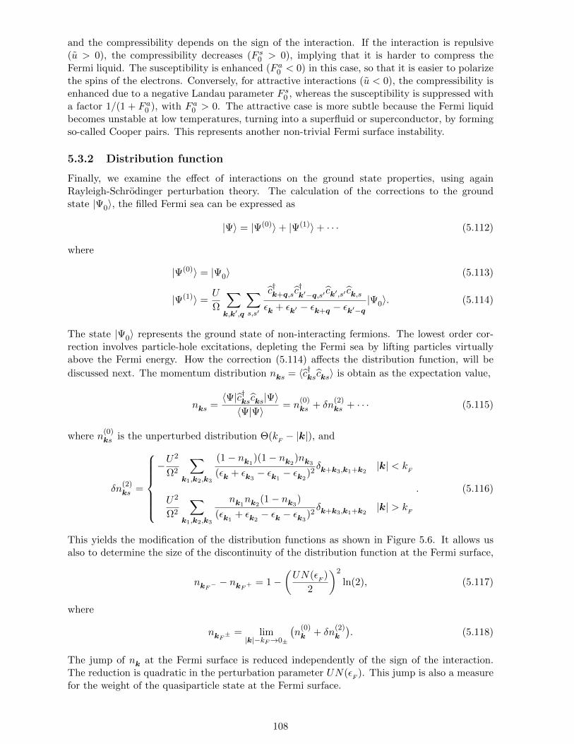
and the compressibility depends on the sign of the interaction. If the interaction is repulsive(u > 0), the compressibility decreases (F s0 > 0), implying that it is harder to compress theFermi liquid. The susceptibility is enhanced (F a0 < 0) in this case, so that it is easier to polarizethe spins of the electrons. Conversely, for attractive interactions (u < 0), the compressibility isenhanced due to a negative Landau parameter F s0 , whereas the susceptibility is suppressed witha factor 1/(1 + F a0 ), with F a0 > 0. The attractive case is more subtle because the Fermi liquidbecomes unstable at low temperatures, turning into a superfluid or superconductor, by formingso-called Cooper pairs. This represents another non-trivial Fermi surface instability.

5.3.2 Distribution function

Finally, we examine the effect of interactions on the ground state properties, using againRayleigh-Schrodinger perturbation theory. The calculation of the corrections to the groundstate |Ψ0〉, the filled Fermi sea can be expressed as

|Ψ〉 = |Ψ(0)〉+ |Ψ(1)〉+ · · · (5.112)

where

|Ψ(0)〉 = |Ψ0〉 (5.113)

|Ψ(1)〉 =U

Ω

∑k,k′,q

∑s,s′

c†k+q,sc†k′−q,s′ ck′,s′ ck,s

εk + εk′ − εk+q − εk′−q|Ψ0〉. (5.114)

The state |Ψ0〉 represents the ground state of non-interacting fermions. The lowest order cor-rection involves particle-hole excitations, depleting the Fermi sea by lifting particles virtuallyabove the Fermi energy. How the correction (5.114) affects the distribution function, will be

discussed next. The momentum distribution nks = 〈c†kscks〉 is obtain as the expectation value,

nks =〈Ψ|c†kscks|Ψ〉〈Ψ|Ψ〉 = n

(0)ks + δn

(2)ks + · · · (5.115)

where n(0)ks is the unperturbed distribution Θ(k

F− |k|), and

δn(2)ks =

−U

2

Ω2

∑k1,k2,k3

(1− nk1)(1− nk2

)nk3

(εk + εk3− εk1

− εk2)2δk+k3,k1+k2

|k| < kF

U2

Ω2

∑k1,k2,k3

nk1nk2

(1− nk3)

(εk1+ εk2

− εk − εk3)2δk+k3,k1+k2

|k| > kF

. (5.116)

This yields the modification of the distribution functions as shown in Figure 5.6. It allows usalso to determine the size of the discontinuity of the distribution function at the Fermi surface,

nkF− − nkF+ = 1−(UN(ε

F)

2

)2

ln(2), (5.117)

where

nkF± = lim|k|−kF→0±

(n

(0)k + δn

(2)k

). (5.118)

The jump of nk at the Fermi surface is reduced independently of the sign of the interaction.The reduction is quadratic in the perturbation parameter UN(ε

F). This jump is also a measure

for the weight of the quasiparticle state at the Fermi surface.

108

1D

Fk

F

nk

nk

kk

3D

k

Figure 5.6: Momentum distribution functions of electrons for a three-dimensional (left panel)and one-dimensional (right panel) Fermion system.

5.3.3 Fermi liquid in one dimension?

Within a perturbative approach the Fermi liquid theory can be justified for a three-dimensionalsystem and we recognize the one-to-one correspondence between bare electrons and quasipar-ticles renormalized by (short-ranged) interactions. Now we would like to show that within thesame approach problems appear in one-dimensional systems, which are conceptional nature andhint that interaction Fermions in one dimension would not form a Fermi liquid, but a Luttingerliquid, as we will motivate briefly below.The Landau parameters have been expressed above in terms of the response functions χ0(q =kF −k′F ) and χ0(q = kF −k′F ). For the one-dimensional system, as given in Eqs.(5.104 - 5.106),the relevant contributions come from two configurations, since there are two Fermi points only(instead of a two-dimensional Fermi surface),

(kF , k′F ) ⇒ q = kF − k′F = 0,±2kF . (5.119)

We find that the response functions show singularities for some of these momenta,10 and weobtain

f↑↑(±kF ,±kF ) = f↓↓(±kF ,∓kF )→∞ (5.122)

as well asf↑↓(kF ,±kF ) = f↓↑(kF ,∓kF )→∞ (5.123)

giving rise to the divergence of all Landau parameters. Therefore the perturbative approach toa Landau Fermi liquid is not allowed for the one-dimensional Fermi system.The same message is obtained when looking at the momentum distribution form which had inthree dimensions a step giving a measure for the (reduced but finite) quasiparticle weight. The

10While χ0(q) is the Lindhard function given in Eq.(3.112) which diverges logarithmically at q = ±2kF , weobtain for the other response function

χ0(q) =

− 2m

~2√

4k2F − q2

ln

(√2kF + q −

√2kF − q√

2kF + q +√

2kF − q

)|q| < 2kF

− 2m

~2√q2 − 4k2

F

(arctan

√q + 2kFq − 2kF

+ arctan

√q − 2kFq + 2kF

)|q| > 2kF

(5.120)

which diverges as

limq→0±

χ0(q) = − m

~2kFln(

q

2kF) , lim

q→2kF−χ0(q) =

m

~2kFand lim

q→2kF+

χ0(q) =πm

~2√

2kF

1√q − 2kF

. (5.121)

109

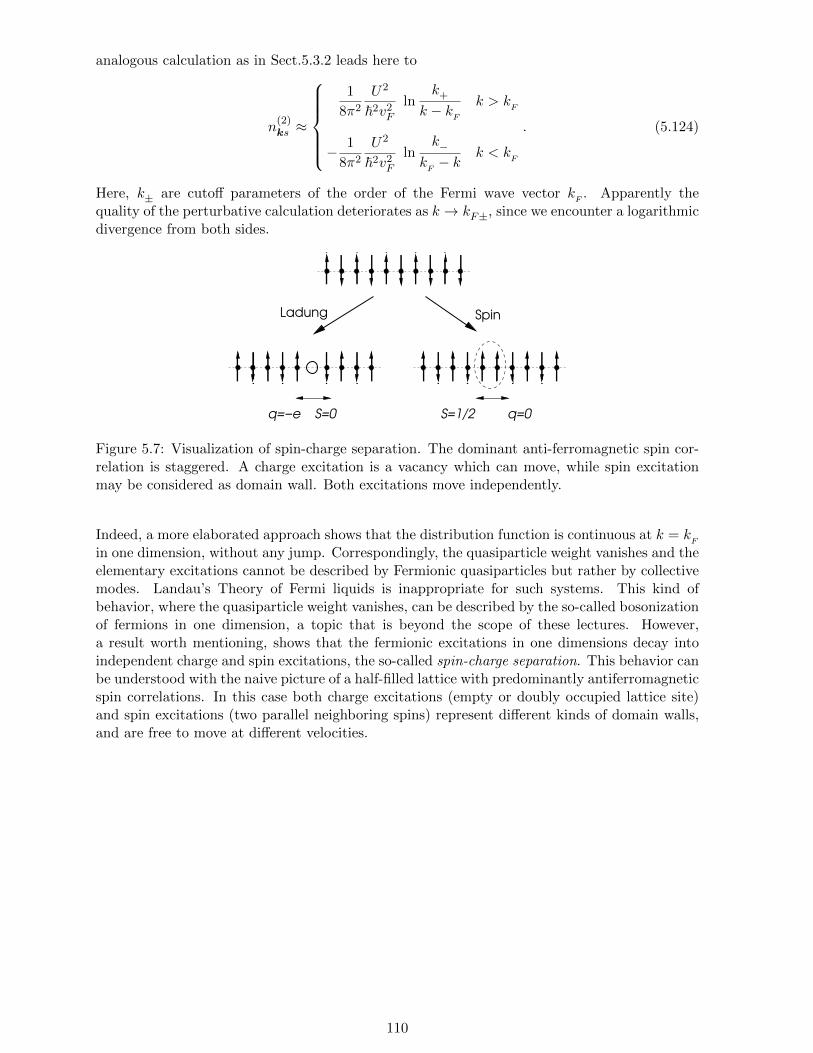
analogous calculation as in Sect.5.3.2 leads here to

n(2)ks ≈

1

8π2

U2

~2v2F

lnk+

k − kF

k > kF

− 1

8π2

U2

~2v2F

lnk−

kF− k k < k

F

. (5.124)

Here, k± are cutoff parameters of the order of the Fermi wave vector kF

. Apparently thequality of the perturbative calculation deteriorates as k → kF±, since we encounter a logarithmicdivergence from both sides.

q=0

SpinLadung

q=−e S=0 S=1/2

Figure 5.7: Visualization of spin-charge separation. The dominant anti-ferromagnetic spin cor-relation is staggered. A charge excitation is a vacancy which can move, while spin excitationmay be considered as domain wall. Both excitations move independently.

Indeed, a more elaborated approach shows that the distribution function is continuous at k = kF

in one dimension, without any jump. Correspondingly, the quasiparticle weight vanishes and theelementary excitations cannot be described by Fermionic quasiparticles but rather by collectivemodes. Landau’s Theory of Fermi liquids is inappropriate for such systems. This kind ofbehavior, where the quasiparticle weight vanishes, can be described by the so-called bosonizationof fermions in one dimension, a topic that is beyond the scope of these lectures. However,a result worth mentioning, shows that the fermionic excitations in one dimensions decay intoindependent charge and spin excitations, the so-called spin-charge separation. This behavior canbe understood with the naive picture of a half-filled lattice with predominantly antiferromagneticspin correlations. In this case both charge excitations (empty or doubly occupied lattice site)and spin excitations (two parallel neighboring spins) represent different kinds of domain walls,and are free to move at different velocities.

110

Chapter 6

Transport properties of metals

The ability to transport electrical current is one of the most remarkable and characteristicproperties of metals. At zero temperature, a ideal pure metal is a perfect electrical conductor,i.e., its resistivity is zero. However, disorder due to impurities and lattice defects influence thetransport and yield a finite residual resistivity, as found in real materials. At finite temperature,electron-electron and electron-phonon scattering lead to a temperature-dependent resistivity.Furthermore, an external magnetic field may influence the resistivity, a phenomenon calledmagnetoresistance, and also leads to the previously studied Hall effect. In this chapter, theeffects of a magnetic field will not be considered. Finally, heat transport, which is also mostlymediated by electrons in metals, is going hand in hand with the electric transport. In thiscontext, transport phenomena such as thermoelectricity (Seebeck and Peltier effect) will beanalyzed here.

6.1 Electrical conductivity

In a normal metal, an electrical current density j(q, ω) (in q, ω-space) is induced by an appliedelectrical field E(q, ω). For a homogeneous isotropic metal, we define the scalar1 electricalconductivity σ(q, ω) within linear response, through

j(q, ω) = σ(q, ω)E(q, ω). (6.1)

The current density j(q, ω) is related to the charge density ρ(r, t) = −en(r, t), via the continuityequation

∂

∂tρ(r, t) + ∇ · j(r, t) = 0, (6.2)

or, in Fourier transformed,

ωρ(q, ω)− q · j(q, ω) = 0. (6.3)

It is interesting to see that a relation between the conductivity σ(q, ω) and the dynamicaldielectric susceptibility χ0(q, ω) defined in equation (3.68) of chapter 3 arises from the equations(6.1) and (6.3). For this, we can calculate

χ0(q, ω) = − ρ(q, ω)

eV (q, ω)= −q · j(q, ω)

eωV (q, ω)

= −σ(q, ω)

ωe

q ·E(q, ω)

V (q, ω)= −σ(q, ω)

ω

[iq2V (q, ω)]

e2V (q, ω). (6.4)

1In an anisotropic material, the conductivity σ would be a full 3× 3 tensor.

111

In the first line, we used the definition (3.68) of χ0(q, ω) and the continuity equation (6.3). Tothe second line, we made use of the definition (6.1) of σ(q, ω) and then replaced E(q, ω) by−iqV (q, ω), which is nothing else than the Fourier transform of the equation

−eE(r, t) = ∇rV (r, t). (6.5)

From this calculations we conclude that

χ0(q, ω) =−iq2

e2ωσ(q, ω), (6.6)

and thus

ε(q, ω) = 1− 4πe2

q2χ0(q, ω) = 1 +

4πi

ωσ(q, ω). (6.7)

In the limit of large wavelengths q kF

, we know from previous discussions2 that ε(0, ω) =1− ω2

p/ω2. Then the conductivity simplifies to

σ(ω) =iω2p

4πω. (6.8)

One might conclude from this result that the conductivity is purely imaginary in the small-qlimit. However, this conclusion is wrong, since the real part of σ(ω) is related to its imaginarypart via the Kramers-Kronig relation. Defining σ1 (σ2) as the real (imaginary) part of σ, thisrelation states that

σ1(ω) = − 1

πP

+∞∫−∞

dω′1

ω − ω′σ2(ω′)

(6.9)

and

σ2(ω) =1

πP

+∞∫−∞

dω′1

ω − ω′σ1(ω′)

. (6.10)

A simple calculation with σ2 from equation (6.8), yields

σ1(ω) =ω2p

4δ(ω), (6.11)

σ2(ω) =ω2p

4πω. (6.12)

Obviously this metal is perfectly conducting (σ → ∞ for ω → 0), which comes from the factthat we considered systems without dissipation so far.An additional important property coming from complex analysis, is the existence of the so-calledf -sum rule,

∞∫0

dω′ σ1(ω′) =1

2

+∞∫−∞

dω′ σ1(ω′) =ω2p

8=πe2n

2m. (6.13)

This relation is valid for all electronic systems (including semiconductors).

2In the small-q limit we approximate χ0(q, ω) ≈ nq2/mω2 from equation (3.82).

112

6.2 Transport equations and relaxation time

We introduce here Boltzmann’s transport theory as as rather simple and efficient way to dealwith dissipation and momentum relaxation of non-stationary electronic states in metals.

6.2.1 The Boltzmann equation

In order to tackle the problem of a finite conductivity, we use a formalism similar to Landau’sFermi liquid theory, based on a distribution function of quasiparticles. In transport theory, thedistribution function can be used to describe the deviation of the system from an equilibrium.If the system is isolated from external influence, equilibrium is reached through relaxation aftersome time, a process which is accompanied with an increase of entropy as discussed in statisticalphysics. Analogously to the theory of transport phenomena, let us introduce the distributionfunction3 f(k, r, t), where

f(k, r, t)d3k

(2π)3d3r (6.14)

is the number of particles in the infinitesimal phase space volume d3rd3k/(2π)3 centered at (k, r),at time t. Such a description is only applicable if the temporal and spacial variations occur atlong wavelengths and small frequencies, respectively, i.e., if typically q k

Fand ~ω ε

F. The

total number of particles N is given by

N = 2

∫d3k

(2π)3d3rf(k, r, t). (6.15)

The equilibrium distribution f0 for the fermionic quasiparticles is given by the Fermi-Diracdistribution,

f0(k, r, t) =1

e(εk−µ)/kBT + 1, (6.16)

and is independent of space r and time t. The general distribution function f(k, r, t) obeys theBoltzmann equation

D

Dtf(k, r, t) =

(∂

∂t+ r ·∇r + k ·∇k

)f(k, r, t) =

(∂f

∂t

)coll

, (6.17)

where the substantial derivative in phase space D/Dt is defined as the total temporal derivativein a frame moving with the phase-space volume. The right-hand side is called collision integraland describes the rate of change in f due to collision processes. Without scattering, the equation(6.17) would represent a continuity equation for f . Now, consider the temporal derivatives of rand k from a quasi-classical viewpoint. In absence of a magnetic field, we find

r =~km, (6.18)

~k = −eE, (6.19)

i.e., the force ~k, which is our central interest, originates from the electric field. The collisionintegral may be expressed via the probability W (k,k′) to scatter a quasiparticle with wavevector k to k′. For simple scattering on static potentials, the collision integral is given by(

∂f

∂t

)coll

= −∫

d3k′

(2π)3

[W (k,k′)f(k, r, t)(1− f(k′, r, t)) (6.20)

−W (k′,k)f(k′, r, t)(1− f(k, r, t))]. (6.21)

3For simplicity we neglect spin the electron spin. In general there would be a distribution function fσ(k, r, t)for each spin species σ.

113

The first term, describing the scattering4 from k to k′, requires a quasiparticle at k, hencethe factor f(k, r, t), and the absence of a particle at k′, therefore the factor 1 − f(k′, r, t).This process describes the scattering out of the phase space volume d3k/(2π)3, i.e., reduces thenumber of particles in it. Therefore, it enters the collision integral with negative sign. Thesecond term describes the opposite process and, according to its positive sign, increases thenumber of particles in the phase space volume d3k/(2π)3. For a system with time inversionsymmetry, we have W (k,k′) = W (k′,k). Assuming this, we can combine both terms and endup with (

∂f

∂t

)coll

=

∫d3k′

(2π)3W (k,k′)

[f(k′, r, t)− f(k, r, t)

]. (6.22)

The Boltzmann equation is a complicated integro-differential equation and suitable approxi-mations are required. Usually, we study processes close to equilibrium, where the deviationf(k, r, t) − f0(k, r, t) is small compared to f(k, r, t). Here, to generalize we assume f0(k, r, t)to be a local equilibrium distribution for which the temperature T = T (r, t) and the chemicalpotential µ = µ(r, t) vary slowly in r and t, such that f0(k, r, t) can still be expressed via the lo-cal Fermi-Dirac distribution (6.16). At small deviations from equilibrium (or local equilibrium),we can approximate the collision integral by the relaxation-time approximation. For simplicity,we assume that the system is isotropic, such that the quasiparticle dispersion εk only dependson |k| and, furthermore, that the scattering probabilities are elastic and depend on the anglebetween k and k′. Then, we make the Ansatz(

∂f

∂t

)coll

= −f(k, r, t)− f0(k, r, t)

τ(εk). (6.23)

The time scale τ(εk) is called relaxation time and gives the characteristic time within which thesystem relaxes to equilibrium.

Consider the simplest case of a system at constant temperature subject to a small uniform electricfield E(t). With f(k, r, t) = f0(k, r, t) + δf(k, r, t), we can calculate the Fourier-transform ofBoltzmann equation (6.17) in relaxation-time approximation and find, after linearizing in δf ,

−iωδf(k, ω)− eE(ω)

~∇kf0(k) = −δf(k, ω)

τ(εk)(6.24)

with

f(k, t) =

∫ +∞

−∞

dω

2πf(k, ω)e−iωt and E(k, t) =

∫ +∞

−∞

dω

2πE(k, ω)e−iωt . (6.25)

In order to come to this expression, we used that f(k, r, t) = f(k, t) for E = E(t) are spaciallyuniform, and assumed for linearizing equation (6.24) that δf ∝ |E|. Thus, the equation (6.24)is consistent to linear order in |E| and can be easily solved as

δf(k, ω) =eτE(ω)

~(1− iωτ)∇kf0(k) =

eτE(ω)

~(1− iωτ)

∂f0(ε)

∂ε∇kεk. (6.26)

This result leads straightforwardly to the quasiparticle current j(ω),

j(ω) = −2e

∫d3k

(2π)3vkf(k, ω) = − e2

4π3

∫d3k

τ(εk)[E(ω) · vk]vk1− iωτ(εk)

∂f0(εk)

∂εk, (6.27)

4Note that if spin was considered here, this collision term would account for scattering processes where spin isconserved. However, there are in principle also scattering process where the electron spin can be transferred tothe lattice (spin-orbit coupling) or an impurity (Kondo effect) and would not be conserved independently.

114

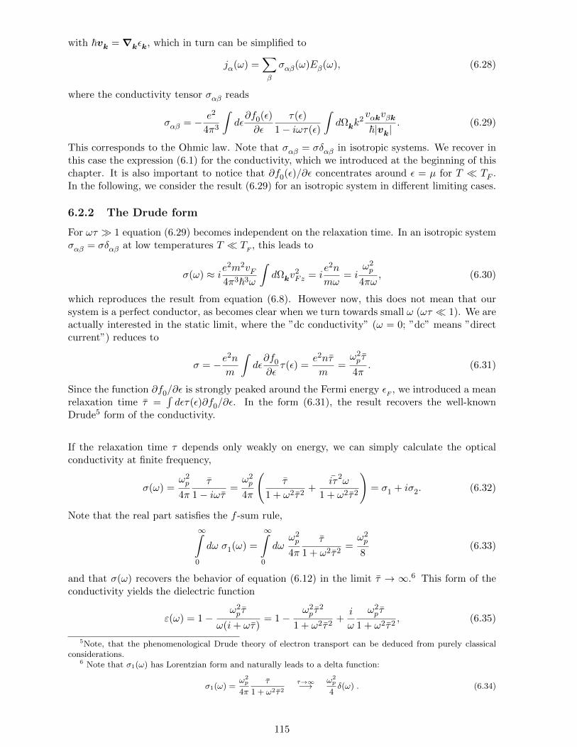
with ~vk = ∇kεk, which in turn can be simplified to

jα(ω) =∑β

σαβ(ω)Eβ(ω), (6.28)

where the conductivity tensor σαβ reads

σαβ = − e2

4π3

∫dε∂f0(ε)

∂ε

τ(ε)

1− iωτ(ε)

∫dΩkk

2vαkvβk~|vk|

. (6.29)

This corresponds to the Ohmic law. Note that σαβ = σδαβ in isotropic systems. We recover inthis case the expression (6.1) for the conductivity, which we introduced at the beginning of thischapter. It is also important to notice that ∂f0(ε)/∂ε concentrates around ε = µ for T TF .In the following, we consider the result (6.29) for an isotropic system in different limiting cases.

6.2.2 The Drude form

For ωτ 1 equation (6.29) becomes independent on the relaxation time. In an isotropic systemσαβ = σδαβ at low temperatures T T

F, this leads to

σ(ω) ≈ ie2m2vF

4π3~3ω

∫dΩkv

2Fz = i

e2n

mω= i

ω2p

4πω, (6.30)

which reproduces the result from equation (6.8). However now, this does not mean that oursystem is a perfect conductor, as becomes clear when we turn towards small ω (ωτ 1). We areactually interested in the static limit, where the ”dc conductivity” (ω = 0; ”dc” means ”directcurrent”) reduces to

σ = −e2n

m

∫dε∂f0

∂ετ(ε) =

e2nτ

m=ω2p τ

4π. (6.31)

Since the function ∂f0/∂ε is strongly peaked around the Fermi energy εF

, we introduced a meanrelaxation time τ =

∫dετ(ε)∂f0/∂ε. In the form (6.31), the result recovers the well-known

Drude5 form of the conductivity.

If the relaxation time τ depends only weakly on energy, we can simply calculate the opticalconductivity at finite frequency,

σ(ω) =ω2p

4π

τ

1− iωτ =ω2p

4π

(τ

1 + ω2τ2+

iτ2ω

1 + ω2τ2

)= σ1 + iσ2. (6.32)

Note that the real part satisfies the f -sum rule,

∞∫0

dω σ1(ω) =

∞∫0

dωω2p

4π

τ

1 + ω2τ2=ω2p

8(6.33)

and that σ(ω) recovers the behavior of equation (6.12) in the limit τ → ∞.6 This form of theconductivity yields the dielectric function

ε(ω) = 1−ω2p τ

ω(i+ ωτ)= 1−

ω2p τ

2

1 + ω2τ2+i

ω

ω2p τ

1 + ω2τ2, (6.35)

5Note, that the phenomenological Drude theory of electron transport can be deduced from purely classicalconsiderations.

6 Note that σ1(ω) has Lorentzian form and naturally leads to a delta function:

σ1(ω) =ω2p

4π

τ

1 + ω2τ2

τ→∞−→ω2p

4δ(ω) . (6.34)

115

which can be used to discuss the optical properties of metals. The complex index of refractionn+ ik is given through (n+ iκ)2 = ε. Next, we discuss three important regimes of frequency.To probe optical properties we consider the reflectivity of light hitting a metal surface perpen-dicularly. Then the reflectivity is given by

R =(n− 1)2 + κ2

(n+ 1)2 + κ2. (6.36)

Inside the metal the light propagation is renormalised by k → k(n+ iκ) with k = ω/c such that

eik(n+iκ)z = eiknze−κkz = eiknze−z/δ (6.37)

defining the penetration length

δ =c

ωκ. (6.38)

Relaxation-free regime (ωτ 1 ωpτ)

In this limit, the real (ε1) and imaginary (ε2) part of the dielectric function (6.35) read

ε1(ω) ≈ −ω2p τ

2, (6.39)

ε2(ω) ≈ω2p τ

ω. (6.40)

The real part ε1 is constant and negative, whereas the imaginary part ε2 becomes singular inthe limit ω → 0. Thus, the refractive index turns out to be dominated by ε2

n(ω) ≈ κ(ω) ≈√ε2(ω)

2≈

√ω2p τ

2ω 1, (6.41)

As a result, the reflectivity R is practically 100%. The absorption index k(ω) determines thepenetration depth δ through

δ(ω) =c

ωκ(ω)≈ c

ωp

√2

ωτ. (6.42)

With this, the skin depth of a metal with the famous relation δ(ω) ∝ ω−1/2 is reproducedwithin the relaxation time approximation of the Boltzmann equation. While length δ(ω) is inthe centimeter range for frequencies of the order of 10− 100Hz, the Debye length c/ωp, is only

of the order of 100A for ~ωp = 10 eV. (cf. Figure 6.1).

Relaxation regime (1 ωτ ωpτ)

Here, we can expand the dielectric function (6.35) in (ωτ)−1, yielding

ε(ω) = 1−ω2p

ω2+ i

ω2p

ω3τ. (6.43)

The real part ε1 ≈ −ω2p/ω

2 is large and negative and dominates in magnitude over ε2. For theoptical properties, we obtain

κ(ω) ≈ωpω

(6.44)

n(ω) ≈ωp

2ω2τ. (6.45)

We find κ(ω) n(ω) 1, which implies a large reflectivity of metals in this frequency range aswell. Note that visible frequencies are part of this regime (see Figures 6.2 and 6.3). The frequencydependence of the penetration depth becomes weak, and its magnitude is approximately givenby the Debye length, δ ∼ c/ωp.

116

Figure 6.1: The frequency dependent reflectivity and penetration depth for ωpτ = 500.

Ultraviolet regime (ω ≈ ωp and ω > ωp)

In this regime, the imaginary part of ε is approximately zero and the real part has the wellknown form

ε1(ω) = 1−ω2p

ω2, (6.46)

such that the reflectivity drops drastically, from close to unity towards zero (cf. Figure 6.1).Metals become nearly transparent in the range ω > ωp. In Figure 6.1, one also notices the rapidincrease in the penetration depth δ, showing the transparency of the metal.

In all these considerations, we have neglected the contributions to the dielectric function due tothe ion cores (core electrons and nuclei). This may be incorporated in Eq.(6.46) in the followingapproximate way:

ε1(ω) = ε∞ −ω2p

ω2, (6.47)

This influences the reflecting properties of metals; particularly, the value of ωp is reduced toω′p = ωp/

√ε∞, where ε∞ is the frequency-independent part of the dielectric function. With this,

the reflectivity for frequencies above ω′p approaches R∞ = (ε∞−1)2/(ε∞+1)2, and 0 < R∞ < 1(see Figure 6.2 and 6.3).

Color of metals

The practically full reflectance for frequencies below ωp is a typical feature of metals. Since formost metals, the plasma frequency lies well above the range of visible light (~ω = 1.5− 3.5eV ),they appear shiny to our eye. While most polished metal surfaces appear shiny white, likesilver, there are some metals with a color, like gold which is yellow and copper which is reddish.White shininess results from reflectance on the whole visible frequency range, while for coloredmetals there is a certain threshold above which the reflectance drops and frequencies towardsblue are not or much weaker reflected. In most cases this drop is not connected with the plasmafrequency, but with light absorption due to interband transitions. Note that the single bandmetal which was used for the Drude theory does not allow for optical absorption apart from theplasma excitation. Interband transition play a particularly important role for the noble metals,Cu, Ag and Au. For these metals, the reflectance drop is caused by the transition from the

117

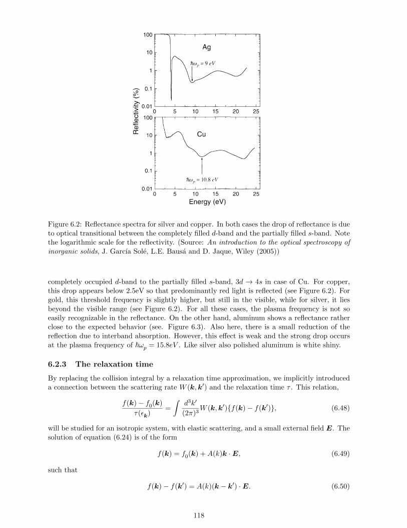
. ri \uollclpoJd eqt ot

" .--,ira aql JoJ sJunocJu

I \: !-'l ]e ueql Je^\ol

-.--. :saql se 'JeAe,^AoH,ulll pue /Y\o[eq spueq

.-:.irlll InJeJ€J e fg't i1r,r.t1ceger ur drP

- -,1 llt sslels 3o lrsuaP'. .rLIt lsoLule le JnJJO

; rrl ruJec eql ^\oleq ,,1rttnd pelleJ-os eql

,,\ JLll.lo ,ltutctn eql ut.- -:: rlll ul dlp eql 'snqJ

. .lelaul uI luelJgJeoJtltlrlsul uI suolllsueJl.1t sa,rt8 'lE '8leue.:.rnitg'lepotu JoIrIuJ

-11 pue Ae E'l lnoqu l€.rrtt rSJd'ulnutulnle JO. a\aqt ozleue oI:.r aql uleldxe urlceds:rrlrur qlIA\ pelelJossu.Ltr alel qJIq^\ 'se8pe

\a t Puu (nJ) ,Le Z!. '(02't) uorlenbg ,(q

.,' iq pa>lretu ueaq e^eq,l'rrL.\\ 'slutod ) pue 1$.

.-.inq eqJ 41'7 arn8tg

A' 8'0t -"rr4

Inc

---l,,I la $="4!t

0y

'Q961'ddrpq4 pueqJIaJuoJqE ruor; uoISSrr-urad qlr,,r,r pecnpo:de:) esec qlee ur peluJrpur sr ,cuanbe:.; eusuld eql olSurpuodse"rroc ,3reue uotod aq1 ':eddoc pue Je^lrs;o erlceds ,(1r,trlcegar aq1 91'p arn8rg

(1e) 6reu39202910190

100

t'0

L

OL

001

L0'0

L'0

L

OL

001

no=oo=.+

\v

0t 9t 0z 9Z

m=/i

,/.\/n

polelnrler '(Ae 6 - dcD4) 3y pue (na 8'0t :'totl) nJ ot Surpuodserrot serSreuauoloqd etuseld eqJ 're^lrs pue teddor Jo eJt3eds 1r,tr1ceger aqt sinoqs 91 'y ern8rg

'slelsru ur suorlrsu€Jl pueqJelul JoeJnleu eql ssnJsrp ol o^uq e,r 'sesueJeJJlp IeJlJeds eseql Jo er.uos JoJ lunocse 01 JepJoul 'urnrtreds elqrsr,t eloq,4A eql ssorre ,lrnrlcegar q8lq,pepurs e s€q tr sr leqt lrolocrelncrged ,(ue lueserd tou seop Jenlrs elrql\ 'lcedse qsrppoJ e seq reddoc pue JoloJqsrmo11e,( e s€q plo8 leql,(11ensrn e,tracred e,nn 'sJorrru poo8 fllereue8 eJe sletetu ]€qltreJ eqt ;o alrds ur 're^.e,4AoH 'elqrsr^ eql ul(lrnrlceger qAIq Jreqt pue uorlerper nIlJoI uorlJe ,Jellg, eql se qJns 'seruedord lereue8 oruos sureldxe ,(11n;sseccns sleleturo! V'V uorlres ur pedolenep (1epou epnrq eqt) lepou uorloole eer; elduls eqJ

STVJSW dO UO'IOJ flHI :JIdOI OEJNIVAOV 8''

orueSo,(rc tB ozrllels,ftc ,1uo'se:nteredruel

,eqr pue (ne 9'IZ ot 9'6 ruo;g) e8uer lecrldo eqt Jo

SCI'IOS CO JNAUVdSNVUI -IVJIJdO EHJ VVI

Figure 6.2: Reflectance spectra for silver and copper. In both cases the drop of reflectance is dueto optical transitional between the completely filled d-band and the partially filled s-band. Notethe logarithmic scale for the reflectivity. (Source: An introduction to the optical spectroscopy ofinorganic solids, J. Garcıa Sole, L.E. Bausa and D. Jaque, Wiley (2005))

completely occupied d-band to the partially filled s-band, 3d → 4s in case of Cu. For copper,this drop appears below 2.5eV so that predominantly red light is reflected (see Figure 6.2). Forgold, this threshold frequency is slightly higher, but still in the visible, while for silver, it liesbeyond the visible range (see Figure 6.2). For all these cases, the plasma frequency is not soeasily recognizable in the reflectance. On the other hand, aluminum shows a reflectance ratherclose to the expected behavior (see. Figure 6.3). Also here, there is a small reduction of thereflection due to interband absorption. However, this effect is weak and the strong drop occursat the plasma frequency of ~ωp = 15.8eV . Like silver also polished aluminum is white shiny.

6.2.3 The relaxation time

By replacing the collision integral by a relaxation time approximation, we implicitly introduceda connection between the scattering rate W (k,k′) and the relaxation time τ . This relation,

f(k)− f0(k)

τ(εk)=

∫d3k′

(2π)3W (k,k′)f(k)− f(k′), (6.48)

will be studied for an isotropic system, with elastic scattering, and a small external field E. Thesolution of equation (6.24) is of the form

f(k) = f0(k) +A(k)k ·E, (6.49)

such that

f(k)− f(k′) = A(k)(k − k′) ·E. (6.50)

118

SEMICONDUCTORS AND INSULATORS r27::-: . : . l le t i l lS-. . : . .horter. , : : - i r than

. rr f t lg

- : . L lp Io__. . t .1nces

: 1 - l - ) ,

*.-- i I

- : .1+

1.0

0.8

a 0.6og 0.4oE

0.2

0.0 1510 2520hot (eV)

Figure 4.5 The reflectivity spectrum of Aluminum (full line) compared with those predictedfrom the ideal metal model with ltato : 15.8 eV (dotted line) and a damped oscillator with f :1.25 x 16ta r-t (dashed line) (experimental data reproduced with permission from Ehrenreichet al.,1962).

In Figure 4.5, the experimental reflectivity spectrum of aluminum is compared withthose predicted by the ideal metal and the damped metal models. Al has a free electrondensity of ly' : 1 8. I x 1922 .*-3 (three valence electrons per atom) and so, accordingtoEquation(4.20),itsplasmaenergyisltc,;o: l5.SeV.Thus,thereflectivityspectrumfor the ideal metal can be now calculated. Compared to the experimental spectrum,the ideal metal model spectrum is only slightly improved when taking into accountthe damping terrn, with f : I.25 x 10la s-1, & value deduced from DC conductivitymeasurements. The main differences between the two calculated spectra are thatdamping produces a reflectivity slightly less than one below op and the ultraviolettransmission edge is slightly smoothed out.

Finally, it should be mentioned that neither the ideal metal model nor the dampedmetal model are able to explain why the actual reflectivity of aluminum is lower thanthe calculated one (R ry 1) at frequencies lower than rt r. Also, these simple modelsdo not reproduce features such as the reflectivity dip observed around 1.5 eV. In orderto account for these aspects, and then to have a better understanding of real metals,the band structure must be taken into account. This will be discussed at the end ofthis chapter, in Section 4.8.

4.5 SEMICONDUCTORS AND INSULATORS

Unlike metals, semiconductors and insulators have bound valence electrons. Thisaspect gives rise to interband transitions. The objective of this and the next section is

Figure 6.3: Reflectance spectrum of aluminum. The slight reduction of reflectivity below ωp isdue to interband transitions. The thin solid line is the theoretical behavior for τ = 0 and thedashed line for finite τ . (Source: An introduction to the optical spectroscopy of inorganic solids,J. Garcıa Sole, L.E. Bausa and D. Jaque, Wiley (2005))

Without loss of generality, we define z ‖ k, and introduce the parametrization of the angles θ,polar angle of E and θ′ (φ′) polar (azimuth) angle of k′), leading to

k ·E = kE cos θ, (6.51)

k · k′ = kk′ cos θ′, (6.52)

k′ ·E = k′E(cos θ cos θ′ + sin θ sin θ′ cosφ′). (6.53)

For elastic scattering, k = k′, we obtain

f(k)− f(k′) = A(k)kE[

cos θ(1− cos θ′)− sin θ sin θ′ cosφ′]. (6.54)

Inserting this into the right-hand side of equation (6.48), the φ′-dependent part of the integrationvanishes for an isotropic system, and we are left with

f(k)− f0(k)

τ(εk)=

∫dΩk′ [f(k)− f(k′)]W (k,k′) (6.55)

= A(k)kE cos θ

∫dΩk′(1− cos θ′)W (k,k′) (6.56)

= [f(k)− f0(k)]

∫dΩk′(1− cos θ′)W (k,k′). (6.57)

The factor [f(k)− f0(k)] can be dropped on both sides of the equation, resulting in

1

τ(εk)=

∫d3k′

(2π)3W (k,k′)(1− cos θ′), (6.58)

where one should remember that, for elastic scattering, the quasiparticle energy εk = εk′ isconserved in the collision process. The scattering probability W (k,k′) accounts for this re-striction. In the next few sections we discuss different scattering processes, looking at collisionprobabilities, relaxation times and the resulting conductivity and resistivity contributions.

6.3 Impurity scattering

6.3.1 Potential scattering

Every deviation from the perfect periodicity of the ionic lattice is a source of quasiparticlescattering, leading to the loss of their original momentum. Without translational invariance,

119

the conservation of momentum is lost, the energy, however, is still conserved. Possible staticscatterers are among others vacancies, dislocations, and impurity atoms. The scattering rateW (k,k′) for a potential V can be determined applying Fermi’s golden rule,7

W (k,k′) =2π

~nimp|〈k′|V |k〉|2δ(εk − εk′). (6.59)

By nimp we denote the density of impurities, assuming only one species of them. For small densi-ties nimp, it is reasonable to neglect interference effects between different impurities. Accordingto equation (6.58), the relaxation time τ of a quasiparticle with momentum ~k is given by

1

τ(εk)=

2π

~nimp

∫d3k′

(2π)3|〈k′|V |k〉|2(1− k · k′)δ(εk − εk′) (6.60)

= nimp(k · vk)

∫dσ

dΩ(k,k′)(1− k · k′)dΩk′

4π, (6.61)

with the differential scattering cross section dσ/dΩ and k = k/|k|. Here, we used the connection8

between Fermi’s golden rule and the Born approximation. Note the difference in the expressionsfor the relaxation time τ in equation (6.58) and for the lifetime τ ,

1

τ=

∫d3k

(2π)3W (k,k′), (6.65)

given by Fermi’s golden rule. The factor (1 − cos θ′) in equation (6.58) gives more weight tobackscattering (θ′ ≈ π) compared to forward scattering (θ′ ≈ 0), since the former has moreinfluence in impeding transport. This explains why τ is also termed transport lifetime.

Assuming defects in the form of point charges Ze, whose screened potential is

〈k′|V |k〉 =4πZe2

|k − k′|2 + k2TF

. (6.66)

In the limit of very strong screening, kTF kF

, the differential cross section becomes inde-pendent of the deviation (k − k′), the transport and the usual lifetime become equal, τ = τ , 9

and

1

τ≈ π

~N(ε

F)nimp

(4πZe2

k2TF

)2

. (6.67)

With this, we are now able to determine the conductivity for scattering on Coulomb defects,assuming s-wave scattering only. Then, since τ(ε) depends weakly on energy, equation (6.31)yields

σ =e2nτ(ε

F)

m, (6.68)

7This corresponds to the first Born approximation in scattering theory. Note, that this approximation isinsufficient to describe resonant scattering.

8The scattering of particles with momentum ~k into the solid angle dΩk′ around k′ yields

W (k,k′)dΩk′ =2π

~Ω

∑k′∈dΩk′

|〈k′|V |k〉|2δ(εk − εk′) (6.62)

=2π

~dΩk′

∫k′∈dΩk′

d3k′

(2π)3〈k′|V |k〉|2δ(εk − εk′) =

2π

~dΩk′N(ε)|〈k′|V |k〉|2. (6.63)

The scattering per incoming particle current jindσ(k,k′) = W (k,k′)dΩk′ determines the differential cross section

k · vkdσ

dΩ(k,k′) =

2π

~N(ε)

4π|〈k′|V |k〉|2. (6.64)

leading to equation (6.61).9In the context of partial wave expansion, one speaks of s-wave scattering, i.e., δl>0 → 0.

120

or, for the specific resistivity ρ = 1/σ,

ρ =m

e2nτ(εF

). (6.69)

Both σ and ρ are independent of temperature. This contribution is called the residual resis-tivity of a metal, which approaches zero for a perfect material. The temperature dependenceof the resistivity is induced in other scattering processes like electron-phonon scattering andelectron-electron scattering, which will be considered below. The so-called residual resistanceratio RRR = R(T = 300K)/R(T = 0) is an often used quantity to benchmark the quality ofa material. It is defined as the ratio between the resistance R at room temperature and theresistance at zero temperature. The bigger the RRR, the better the quality of the material.The typical value of RRR for common copper is 40-50, while the RRR for very clean aluminumreaches values up to 20000.

6.3.2 Kondo effect

There are impurity atoms inducing so-called resonant scattering. If the resonance occurs close tothe Fermi energy, the scattering rate is strongly energy dependent, inducing a more pronouncedtemperature dependence of the resistivity. An important example is the scattering off magneticimpurities with a spin degree of freedom, yielding a dramatic energy dependence of the scatteringrate. This problem was first studied by Kondo in 1964 in order to explain the peculiar minimain resistivity in some materials. The coupling between the local spin impurities Si at Ri andthe quasiparticle spin s has the exchange form

VK

=∑i

(VK

)i

= J∑i

Si · s(r)δ(r −Ri) (6.70)

= J∑i

(Szi s

z(r) +1

2S+i s−(r) +

1

2S−i s

+(r)

)δ(r −Ri) (6.71)

=J~2Ω

∑k,k′,i

[Szi (c†k↑ck′↑ − c

†k↓ck′↓) + S+

i c†k↓ck′↑ + S−i ck↑ck′↓

]e−i(k−k

′)·Ri . (6.72)

Here, it becomes important that spin flip processes, which change the spin state of the impurityand that of the scattered electron, are enabled. The results for the scattering rate are presentedhere without derivation,

W (k,k′) ≈ J2S(S + 1)

[1 + 2JN(ε

F) ln( D

|εk − εF |)], (6.73)

where D is the bandwidth and we have assumed that JN(εF

) 1. The relaxation time is foundto be

1

τ(εk)≈ J2S(S + 1)

~N(ε)

[1 + 2JN(ε

F) ln( D

|εk − εF |)]. (6.74)

Note that W (k,k′) does not depend on angle, meaning that the process is described by s-wavescattering. The energy dependence is singular at the Fermi energy, indicating that we are notdealing with simple resonant potential scattering, but with a much more subtle many-particleeffect involving the electrons very near the Fermi surface. The fact that the local spins Sican flip, makes the scattering center dynamical, because the scatterer is constantly changing.The scattering process of an electron is influenced by previous scattering events, leading to thesingularity at ε

F. This cannot be described within the first Born approximation, but requires

at least the second approximation or the full solution.10 As mentioned before, the resonant

10We refer to J.M. Ziman, Principles of the Theory of Solids, and A.C. Hewson, The Kondo Problem to HeavyFermions for more details.

121

behavior induces a strong temperature dependence of the conductivity. Indeed,

σ(T ) =e2k3

F

6π2m

∫dε

1

4kBT cosh2(ε− ε

F)/2k

BT )τ(ε) (6.75)

≈ e2n

8mkBT

∫dεJ2S(S + 1)[1− 2JN(ε

F) ln(D/ε)]

cosh2(ε/2kBT )

. (6.76)

A simple substitution in the integral leads to

σ(T ) ≈ e2n

2mJ2S(S + 1)

[1− 2JN(ε

F) ln( D

kBT

)]. (6.77)

Usual contributions to the resistance, like electron-phonon scattering discussed below, typicallydecrease with temperature. The contribution (6.77) to the conductivity is strongly increas-ing, inducing a minimum in the resistance, when we crossover from the decreasing behaviorat high temperatures to the low-temperature increase of ρ(T ). At even lower temperatures,the conductivity would decrease and eventually even turn negative which is an artifact of ourapproximation. In reality, the conductivity saturates at a finite value when the temperature islowered below a characteristic Kondo temperature T

K,

kBTK

= De−1/JN(εF ), (6.78)

a characteristic energy scale of this system. The real behavior of the conductivity at temperaturesT T

Kis not accessible by simple perturbation theory. This regime, known as the Kondo

problem, represents one of the most interesting correlation phenomena of many-particle physics.

6.4 Electron-phonon interaction

Even in perfect metals, the conductivity becomes non-zero at finite temperature. The thermallyinduced distortions of the lattice, phonons, act as fluctuating scattering centers. In the languageof electron-phonon interaction, electrons are scattered via absorption and emission of phonons,which induce local fluctuations in volume (cf. Chapter 3). The corresponding coupling termwas given in equation (3.143) and simplifies with the definition (3.130) to

Hint = 2i∑k,q,s

Vq

√~

2ρ0ωq|q|(bq − b

†−q)c

†k+q,scks. (6.79)

The interaction is formally similar to the coupling between electrons and photons. The dominantprocesses consist of single-phonon processes, i.e., the absorption or emission of one phonon. En-ergy and momentum are conserved, such that, for the scattering of an electron from momentumk to k′ due to the emission of a phonon with momentum q, we have

k = k′ + q +G, (6.80)

εk = ~ωq + εk′ , (6.81)

Here, ωq = csq is the phonon spectrum, while the reciprocal lattice vector G allows for scat-

tering11 in nearby Brillouin zones. By this, the phase space available for scattering is stronglyreduced, especially near the Fermi energy. Note that ~ωq ≤ ~ω

D ε

F. In order to calculate

11This so-called Umklapp phenomenon will be discussed in some more detail later in this chapter.

122

the scattering rates, the matrix elements12 of the available processes,

〈k + q;Nq′ |(bq − b†−q)c

†k+q,scks|k;N ′q′〉 = 〈k + q|c†k+q,scks|k〉

(√N ′q′ δNq′ ,N

′q′−1 δq,q′

−√N ′q′ + 1 δNq′ ,N

′q′+1 δq,−q′

),

(6.82)

need to be calculated. From Fermi’s golden rule we obtain(∂f

∂t

)coll

= −2π

~∑q

|g(q)|2[[f(k)(1− f(k + q))(N−q + 1)

− f(k + q)(1− f(k))N−q]δ(εk+q − εk + ~ω−q)

−[f(k + q)(1− f(k))(Nq + 1)

− f(k)(1− f(k + q))Nq]δ(εk+q − εk − ~ωq)

], (6.83)

where g(q) = Vq|q|√

2~/ρ0ωq. Each of these four terms describes one of the single phonon

scattering processes depicted in Figure 6.4.

−q

k

k + q

k + q

k k

k + q

k + q

k

−q q q

Figure 6.4: The four single-phonon electron-phonon scattering processes.

The collision integral leads to a complicated integro-differential equation, whose solution is te-dious and would involve the solution of the non-equilibrium phonon-problem as well. Instead ofa full rigorous calculation including the non-equilibrium redistribution of phonons, we will con-sider the behavior in various temperature regimes by an approximate treatment of the phonons.The characteristic temperature of phonons, the Debye temperature Θ

D T

F, is much smaller

than the Fermi temperature. Hence, the phonon energy is virtually unimportant for the en-ergy conservation, εk′=k+q ≈ εk. Therefore we are allowed to impose momentum conservationεk+q = εk and consider the lattice distortion as being essentially static, in the sense of anadiabatic Born-Oppenheimer approximation. The approximate collision integral then reads(

∂f

∂t

)coll

=2π

~∑q

|g(q)|22N(ωq)[f(k + q)− f(k)]δ(εk+q − εk), (6.84)

where we assume the occupation of phonon states according to the equilibrium distribution forbosons,

N(ωq) =1

e~ωq/kBT − 1. (6.85)

This approximation includes all important aspects of the electron-phonon scattering we need toderive the temperature dependence of ρ(T ).

12In analogy to the discussion on electromagnetic radiation, the phenomenon of spontaneous phonon emissiondue to zero-point fluctuations appears. It is formally visible in the additional “+1” in the factors (N±q) + 1.

123

In analogy to previous approaches, we obtain for with relaxation-time Ansatz

1

τ(εk)=

2π

~λ

N(εF

)

∫d3q

(2π)3~ωqN(ωq)(1− cos θ)δ(εk+q − εk), (6.86)

where |k| = |k + q| = kF

, meaning that only the electrons in a thin shell close to the Fermisurface are relevant. Furthermore, we parametrized g(q) according to

|g(q)|2 =λ

2N(εF

)Ω~ωq, (6.87)

where λ is a dimensionless electron-phonon coupling constant. In usual metals λ < 1. As in thecase of defect scattering, the relaxation time depends only weakly on the electron energy. But,unlike previously, the direct temperature dependence enters via the dependence on temperatureof the phonon occupation N(ωq).

q

kFk

k + q

γ

θ

Figure 6.5: The geometry of electron-phonon scattering.

In order to perform the integration in equation (6.86), we have to re-express δ(εk+q − εk) bywriting

δ(εk+q − εk) = δ

(~2

2m(q2 − 2k

Fq cos γ)

)=

m

~2kFqδ

(q

2kF

− cos γ

), (6.88)

where γ is defined in Figure 6.5. From there, we also see that 2γ + θ = π, and thus, find therelation

1− cos θ = 1 + cos(2γ) = 2 cos2(γ). (6.89)

Obviously, we have to integrate q over the range [0, 2kF

] on the right-hand side of equation(6.86), which can be reformulated to

1

τ(εF , T )=−λN(ε

F)

m

~2πkF

2kF∫0

dq qωqN(ωq)

π/2∫0

dγ sin γ cos2(γ) δ( q

2kF

− cos γ)

(6.90)

=λ

4N(εF

)

mcs~2πk3

F

2kF∫0

q4dq

e~csq/kBT − 1(6.91)

=λ

4N(εF

)

mcsk2F

~2π

(T

ΘD

)52ΘD/T∫

0

y4dy

ey − 1, (6.92)

124

where we have approximated the Debye temperature by kB

ΘD≈ 2~cskF . We notice the two

distinct characteristic temperature regimes,

1

τ=

6ζ(5)λπ

kB

ΘD

~

(T

ΘD

)5

, T ΘD,

λπkB

ΘD

~

(T

ΘD

), T Θ

D.

(6.93)

The prefactors depend on the details of the approximation, whereas the qualitative temperaturedependence does not. We finally obtain the conductivity and resistivity from equation (6.29),

σ =e2n

mτ(T ), (6.94)

ρ =m

e2n

1

τ(T ), (6.95)

where we used the weak energy dependence of τ(ε ≈ εF, T ). With this, we obtain the well-known

Bloch-Gruneisen form

ρ(T ) ∝

T 5, T ΘD,

T, T ΘD.

(6.96)

At high temperatures, ρ is determined by the occupation of phonon states

N(ωq) ≈kBT

~ωq(6.97)

which change the scattering strength (amplitude) of the lattice modulation linear in T . At lowtemperature only the lowest phonon states are occupied ~ωq < kBT yield q < kBT/~cs. Thus, atlow temperatures only long-wave length modulations of the lattice generate a scattering poten-tials which deflects electrons only slightly from their trajectories (forward scattering dominates).This represents a restriction of the scattering phase space becoming ever smaller with decreasingtemperature.

6.5 Electron-electron scattering

In Chapter 5 we have learned, that, taking a short-ranged electron-electron interaction intoaccount, the lifetime of a quasiparticle strongly increases close to the Fermi surface. The basicreason was the constraint of the scattering phase space due to the Pauli principle. The lifetime,which we can identify with the relaxation time here, has the form

1

τ(ε)∝ (ε− ε

F)2. (6.98)

Note that this phase space reduction does not restrict the momentum transfer, so that in prin-ciple 0 < q < 2kF is valid for all energies ε. This allows determining the conductivity fromequation (6.29), and we find

σ(T ) ∝ 1

T 2(6.99)

The resistivity ρ ∝ T 2 increases quadratically in T . This is a key property of a Fermi liquid andis often considered an identifying criterion.

125

Umklapp process

An important point, kept quiet so far, requires some explanation. One could argue, that themomentum of the Fermi liquid is conserved upon the collision of two electrons. With thisargument, it is not quite clear what causes a finite resistance. This argument, however, is basedon translational invariance and ignores the existence of the underlying lattice. In the sense thatthe kinematics (momentum conservation) is also satisfied for electrons being scattered from theFermi surface of one Brillouin zone to the one of another Brillouin zone, while incorporating areciprocal lattice vector. The equation of momentum conservation,

k = k′ +G, (6.100)

where G is a reciprocal vector of the lattice, allows for scattering to other Brillouin zones(G 6= 0). By this, the momentum is transferred to a static deformation of the lattice. Such pro-cesses are termed Umklapp processes and play an important role in electron-phonon scatteringas well (see equation (6.80)).

1st$Brillouin$zone$~k

~k + ~q

~k0 ~q

~k0 ~k00

~k00 ~q

Umkplapp$$sca4ering$

ordinary$sca4ering$

Figure 6.6: Considering energy and momentum conservation in two-electron collision there areordinary scattering processes (k,k′) → (k + q,k′ − q) which does not lead to a momentumrelaxation, and there are Umklapp scattering processes (k,k′′) → (k + q,k′′ − q) leading to aneighbouring Brillouin zone, here visualized by an extended Brillouin zone scheme.

6.6 Matthiessen’s rule and the Ioffe-Regel limit

Matthiessen’s rule states, that the scattering rates of different scattering processes can simplybe added, leading to

W (k,k′) = W1(k,k′) +W2(k,k′), (6.101)

or, expressed in the relaxation time approximation,

1

τ=

1

τ1

+1

τ2

, (6.102)

and

ρ =m

ne2τ=

m

ne2

(1

τ1

+1

τ2

)= ρ1 + ρ2. (6.103)

126

This rule is not a theorem and corresponds effectively to a serial coupling of resistors in a clas-sical circuit. It is applicable, if the different scattering processes are independent. Actually,the assumption that the impurity scattering rate depends linearly on the impurity density nimp

is already an application of Matthiessen’s rule. Mutual influences of impurities, e.g., throughinterference effects due to the coherent scattering of an electron at different impurities, would in-validate this simplification. An example where Matthiessen’s rule is violated is a one-dimensionalsystem, where a single scatterer i induces a finite resistance Ri. Two serial scatterers then leadto a total resistance

R = R1 +R2 +2e2

hR1R2 ≥ R1 +R2. (6.104)

The reason is, that in one-dimensional systems, the interference of backscattered waves is un-avoidable and no impurity can be treated as isolated. Furthermore, every particle traversing thewhole system has to pass all scatterers. The more general Matthiessen’s rule,

ρ ≥ ρ1 + ρ2, (6.105)

is still valid. Another source of deviation from Matthiessen’s rule arises, if the relaxation timedepends on k, since then the averaging is not the same for all scattering processes. The electron-phonon coupling can be modified by the scattering on impurities, most importantly in thepresence of anisotropic Fermi surfaces. For the analysis of resistance data of simple metals, weoften assume the validity of Matthiessen’s rule. A typical example is the resistance minimumexplained by Kondo, where

ρ(T ) = ρ0 + ρe−p(T ) + ρK

(T ) + ρe−e(T ) (6.106)

= ρ0 + αT 5 + β(1 + 2JN(εF

) ln(D/kBT )) + γT 2, (6.107)

where α, β, and γ are numerical constants. Upon decreasing temperature, the Kondo term isincreasing, whereas the electron-phonon and electron-electron contributions decrease. Conse-quently, there is a minimum.

We now turn to the discussion of resistivity in the high-temperature limit. Believing the previousconsiderations entirely, the electrical resistivity would grow indefinitely with temperature. Inmost cases, however, the resistivity will saturate at a finite limiting value. We can understandthis from simple considerations writing the mean free path ` = vF τ(ε

F) as the mean distance an

electron travels freely between two collisions. The lattice constant a is a natural lower boundaryto ` in the crystal lattice. Furthermore, we assumed so far that scattering occurs between twostates with sharp momenta k and k′. If the de Broglie wavelength becomes comparable to themean free path, the framework becomes unfounded and k−1

Fwould become a boundary for `. In

most systems a and k−1F

are comparable lengths. Empirically, the resistivity is described via theformula

1

ρ(T )=

1

ρBT

(T )+

1

ρmax

, (6.108)

corresponding to the parallel addition of two resistivities; on one hand, ρBT

(T ), which we haveinvestigated using the Boltzmann transport theory, and on the other hand the limiting valueρmax. This is in clear disagreement to Matthiessen’s rule, which is to be expected, since forkF` ∼ 1, complex interference effects will arise. The saturated resistivity ρmax can be estimated

from the Jellium model,

ρmax =m

e2nτ(εF

)=

3π2m

e2k3Fτ(ε

F)

=h

e2

3π

2k2F`

(6.109)

∼ h

e2

3π

2kF

, (6.110)

127

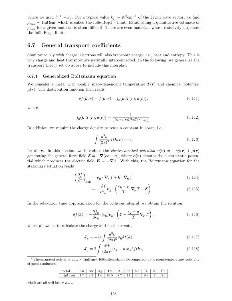
where we used `−1 ∼ kF

. For a typical value kF∼ 108cm−1 of the Fermi wave vector, we find

ρmax ∼ 1mΩcm, which is called the Ioffe-Regel13 limit. Establishing a quantitative estimate ofρmax for a given material is often difficult. There are even materials whose resistivity surpassesthe Ioffe-Regel limit.

6.7 General transport coefficients

Simultaneously with charge, electrons will also transport energy, i.e., heat and entropy. This iswhy charge and heat transport are naturally interconnected. In the following, we generalize thetransport theory set up above to include this interplay.

6.7.1 Generalized Boltzmann equation

We consider a metal with weakly space-dependent temperature T (r) and chemical potentialµ(r). The distribution function then reads

δf(k; r) = f(k; r)− f0(k, T (r), µ(r)), (6.111)

where

f0(k, T (r), µ(r)) =1

e(εk−µ(r))/kBT (r) + 1. (6.112)

In addition, we require the charge density to remain constant in space, i.e.,∫d3k

(2π)3f(k; r) = n0 (6.113)

for all r. In this section, we introduce the electrochemical potential η(r) = −eφ(r) + µ(r)generating the general force field E = −∇(eφ+ µ), where φ(r) denotes the electrostatic poten-tial which produces the electric field E = −∇φ. With this, the Boltzmann equation for thestationary situation reads(

∂f

∂t

)coll

= vk ·∇r f + k ·∇k f (6.114)

= − ∂f∂εk

vk ·(εk − µT

∇r T − E). (6.115)

In the relaxation time approximation for the collision integral, we obtain the solution

δf(k) = −∂f0

∂εkτ(εk)vk ·

(E − εk − µ

T∇r T

), (6.116)

which allows us to calculate the charge and heat currents,

Je = −2e

∫d3k

(2π)3vkδf(k), (6.117)

Jq = 2

∫d3k

(2π)3(εk − µ)vkδf(k), (6.118)

13The saturated resistivity ρmax ∼ 1mΩcm= 1000µΩcm should be compared to the room-temperature resistivityof good conductors,

metal Cu Au Ag Pt Al Sn Na Fe Ni Pb

ρ [µΩcm] 1.7 2.2 1.6 10.5 2.7 11 4.6 9.8 7 21

which are all well below ρmax.

128

x x

yy

b)a)

k

k

k

δ

k

fkδf

k

Figure 6.7: Schematic view of the distribution functions δf(k) on a slice cut through the k-space(kz = 0) with a circular Fermi surface for two situations. On the left panel (a), for an appliedelectric field along the negative x-direction, on the right panel (b) for a temperature gradient inx-direction.

respectively. Inserting the solution (6.116) into the two definitions above yields

Je = eK(0)E − e

TK(1) (−∇T ) , (6.119)

Jq = −K(1)E +1

TK(2) (−∇T ) , (6.120)

where ∇ should be understood as ∇r and the tensors K(n) (n ∈ N0) are defined as

K(n)αβ = − 1

4π3

∫dε

∂f0

∂ετ(ε)(ε− µ)n

∫dΩk

vFαvFβ~|v

F| k

2F. (6.121)

For an isotropic system these transport coefficients are no longer tensors but represented byscalars,

K(n) = −n0

m

∫dε

∂f0

∂ετ(ε)(ε− µ)n (6.122)

In the case T TF

we can calculate the coefficients,14

K(0)(εF

) =n0(ε

F)τ(ε

F)

m(6.125)

K(1)(εF

) =π2

3(k

BT )2 ∂

∂εK(0)(ε)

∣∣∣∣ε=εF

, (6.126)

K(2)(εF

) =π2

3(k

BT )2K(0)(ε

F). (6.127)

We measure the electrical resistivity assuming thermal equilibrium, ∇T = 0 for all r. Withthis, we find the expression

σ = e2K(0). (6.128)

14If a function g(ε) depends only weakly on ε in the vicinity of εF , we can use the Sommerfeld (Taylor) expansionto derive a general approximation for following integrals

−∫dεg(ε)

∂f0

∂ε= g(εF ) +

π2

6(kBT )2 ∂2g(ε)

∂ε2

∣∣∣∣ε=εF

+ . . . (6.123)

and

−∫dεg(ε)(ε− εF )

∂f0

∂ε=π2

3(kBT )2 ∂g(ε)

∂ε

∣∣∣∣ε=εF

+ . . . , (6.124)

in the limit T → 0. We used that µ→ εF in that asymptotic case.

129

In order to determine the thermal conductivity κ relating the heat current Jq to ∇T when noexternal electric field E is applied, we set Je = 0 as for an open circuit. Then, the equations(6.119) and (6.120) reveal the appearance of an general force field

E = − K(1)

TK(0)∇T. (6.129)

Thus, the heat current is given by

Jq = − 1

T

(K(2) − K(1)2

K(0)

)∇T = −κ∇T. (6.130)

In simple metals, the second term in (6.130) is often negligible as compared to the first one andwe obtain in this case

κ =1

TK(2) =

π2k2B

3TK(0) =

π2

3

k2B

e2T σ, (6.131)

which is the well-known Wiedemann-Franz law. Note, that we can write the thermal conductivityin the form

κ =C

e2N(εF

)σ, (6.132)

where C = π2N(εF

)k2BT/3 denotes the electronic specific heat.

6.7.2 Thermoelectric effect

Equation (6.129) shows, that a temperature gradient induces an electric field. For a simple,isotropic system, this relation reduces to

E = Q∇T = − K(1)

TK(0)∇T, (6.133)

with the Seebeck coefficient

Q = − π2

3

k2BT

e

σ′(ε)σ(ε)

∣∣∣∣ε=εF

. (6.134)

This is the so-called Mott formula which looses its validity at high-temperatures or very anisotropicscattering. Using σ(ε) = n(ε)e2τ(ε)/m, we investigate σ′(ε),

σ′(ε) =τ ′(ε)τ(ε)

σ(ε) +n′(ε)n(ε)

σ(ε) =τ ′(ε)τ(ε)

σ(ε) +N(ε)

n(ε)σ(ε), (6.135)

and obtain an additional contribution to Q, if the relaxation time depends strongly on energy.This is most prominent in collision processes in which resonant scattering is involved (e.g., theKondo effect). In the opposite situation, namely, when the first term is irrelevant, the Seebeckcoefficient

Q = −π2

3

k2BT

e

N(εF

)

n(εF

)= − S

ne(6.136)

is simply reduced to the entropy per electron. For simple metals such as the alkali metals wemay estimate the low-temperature values using equation (6.136)

Q = −π2

2

k2BT

eεF= −π

2

2

kBT

eTF(6.137)

which for TF (Na,K) ≈ 3 × 104K leads to Q = −14nV K−1 × T [K]. A comparison withexperiments in Fig.6.8 shows that the order of magnitude works reasonably well for Na and K.However, for Li and Cs even the sign is different. Differences occur through phonon effects, suchas the so-called phonon drag which we have neglected here.In the following, we consider two different types of thermoelectric effects.

130

Q [

nV

/K]

T [K]

100

0

K

Na

LiCs

1 2

0

−50

50

Figure 6.8: Seebeck coefficient for the Alkali metals Li, Na, K, and Cs at low temperatures. Thedashed line represents the estimate for Na and K following Eq.(6.137). (adapted from D.K.C.MacDonald, Thermoelectricity: an introduction to the principles, Dover (2006).)

Seebeck effect

The first is the Seebeck effect, where a thermoelectric voltage appears in a bi-metallic system(cf. Figure 6.9). With equation (6.133), a temperature gradient across metal B induces anelectromotive force15

UEMF

=

∫dl · E (6.138)

= QA

T1∫T0

dl ·∇T +QB

T2∫T1

dl ·∇T +QA

T0∫T2

dl ·∇T (6.139)

= (QB−Q

A)(T2 − T1). (6.140)

The resulting voltage Vtherm = UEMF

appears between the two ends of a second metal A, whosecontacts are kept at the same temperature T0. Here, a bi-metallic configuration was chosen toreveal voltage differences across the contacts which are absent in a single metal.

15The term electromotive force, first introduced by Alessandro Volta, is misleading in the sense, that it measuresa voltage instead of a force.

131

a) b)

metal A

metal A

metal B

metal A

metal A

metal BE

T1

T2

T0

T0 T0

T0 T0

T0

Vtherm Je Je

Jq

Jq

Figure 6.9: Schematics of thermoelectric effects. On the left panel (a) a representation of Seebeckeffect is given, where the symbol E is used instead of E . On the right panel (b) the Peltier effectis represented. In our analysis, both systems were effectively one-dimensional.

Peltier effect

The second phenomenon, termed Peltier effect, emerges in a system kept at the same temper-ature everywhere. Here, an electric current Je between the two contacts of the metal A (seeFigure 6.9) induces a heat current in the bi-metallic system, such that heat is transferred fromone reservoir (top) to another (bottom). This follows from the equations (6.119) and (6.120) byassuming ∇T = 0, where

Je = e2K(0)E

Jq = −K(1)E

(6.141)

implies

Jq = −K(1)

K(0)Je = ΠJe = QTJe. (6.142)

The coupling Π = TQ between Jq and Je is called Peltier coefficient. According to Figure 6.9,a contribution to the heat current is to be expected from both metals A and B,

Jq = (ΠA−Π

B)Je = T0(Q

A−Q

B)Je. (6.143)

This means, that the heat transfer between reservoirs can be controlled by electrical current.

It has to be emphasized here that the bi-metal design of the devices in Fig. 6.9 serves theobservation of the two effects which both represent bulk effects of the two metals A and B. Byno means, it should be mistaken as an effect originating from the inter-metal contacts.

6.8 Anderson localization in one-dimensional systems

Transport in one spatial dimension is very special, since there are only two different directionsto go: forward and backward. We introduce the transfer matrix formalism and use it to expressthe conductivity through the Landauer formula. We will then investigate the effects of multiplescattering at different obstacles, leading to the so-called Anderson localization, which turns ametal into an insulator.

6.8.1 Landauer Formula for a single impurity

The transmission and reflection at an arbitrary potential with finite support16 in one dimensioncan be described by a transfer matrix T .

16The support (dt. Trager) of a function is the set of all points, where the function takes non zero values.

132

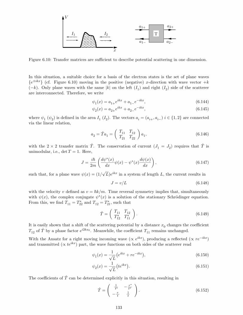
x

I1 I2

a1+ a2+

V

a1− a2−

T

Figure 6.10: Transfer matrices are sufficient to describe potential scattering in one dimension.

In this situation, a suitable choice for a basis of the electron states is the set of plane wavese±ikx (cf. Figure 6.10) moving in the positive (negative) x-direction with wave vector +k(−k). Only plane waves with the same |k| on the left (I1) and right (I2) side of the scattererare interconnected. Therefore, we write

ψ1(x) = a1+eikx + a1−e

−ikx, (6.144)

ψ2(x) = a2+eikx + a2−e

−ikx, (6.145)

where ψ1 (ψ2) is defined in the area I1 (I2). The vectors ai = (ai+, ai−) i ∈ 1, 2 are connectedvia the linear relation,

a2 = T a1 =

(T11 T12

T21 T22

)a1, (6.146)

with the 2 × 2 transfer matrix T . The conservation of current (J1 = J2) requires that T isunimodular, i.e., detT = 1. Here,

J =i~2m

(dψ∗(x)

dxψ(x)− ψ∗(x)

dψ(x)

dx

), (6.147)

such that, for a plane wave ψ(x) = (1/√L)eikx in a system of length L, the current results in

J = v/L (6.148)

with the velocity v defined as v = ~k/m. Time reversal symmetry implies that, simultaneouslywith ψ(x), the complex conjugate ψ∗(x) is a solution of the stationary Schrodinger equation.From this, we find T11 = T ∗22 and T12 = T ∗21, such that

T =

(T11 T12

T ∗12 T ∗11

). (6.149)

It is easily shown that a shift of the scattering potential by a distance x0 changes the coefficient

T12 of T by a phase factor ei2kx0 . Meanwhile, the coefficient T11 remains unchanged.

With the Ansatz for a right moving incoming wave (∝ eikx), producing a reflected (∝ re−ikx)and transmitted (∝ teikx) part, the wave functions on both sides of the scatterer read

ψ1(x) =1√L

(eikx + re−ikx

), (6.150)

ψ2(x) =1√L

(teikx

). (6.151)

The coefficients of T can be determined explicitly in this situation, resulting in

T =

(1t∗ − r∗

t∗

− rt

1t

). (6.152)

133

Here, the conservation of currents imposes the condition 1 = |r|2 +|t|2. Furthermore, we can finda relation between the parameters (r, t) of the potential barrier and the electric resistivity. Forthis, we notice that the incoming current density J0 is split into a reflected Jr and transmittedJt part, all given by

J0 = − 1

Lve = −n0ve, (6.153)

Jr = −|r|2

Lve = −nrve, (6.154)

Jt = −|t|2

Lve = −ntve, (6.155)

with the velocity v = ~k/m, the electron charge −e, and the particle densities n0, nr, and ntcorresponding to the incoming, reflected and transmitted particles respectively. The electrondensity on the two sides of the barrier is given by

n1 = n0 + nr =1 + |r|2L

, (6.156)

n2 = nt =|t|2L. (6.157)

From this consideration, a density difference δn = n1−n2 = (1 + |r|2− |t|2)/L = 2|r|2/L resultsbetween the left and the right side of the scatterer. The resistance R of the barrier is definedby the ratio between the voltage drop over the resistor δV and the transmitted current Jt, i.e.

R =δV

Jt(6.158)

Consequently, a relation between δV and the electron density δn remains to be established todetermine R. The connection is easily found via the existing energy difference δE = −eδVbetween the two sides of the resistor, such that the expression

δn =dn

dEδE (6.159)

=dn

dE(−eδV ) (6.160)

produces the wished relation. Here, dndEdE is the number of states per unit length in the energy

interval [E,E + dE] and we find

dn

dE=

1

L

∑k,s

δ

(E − ~2k2

2m

)= 2

∫dk

2πδ

(E − ~2k2

2m

)=

1

π~v(E). (6.161)

The resistance R is finally obtained from the equations (6.158), (6.159), and (6.161), leading to

R =h

e2

|r|2|t|2 , (6.162)

The Klitzing constant RK

= h/e2 ≈ 25.8kΩ is a resistance quantum named after the discovererof the Quantum Hall Effect. The result (6.162) is the famous Landauer formula, which isvalid for all one-dimensional systems and whose application often extends to the description ofmesoscopic systems and quantum wires.

134

T T1 2

Figure 6.11: Two spatially separated scattering potentials with transmission matrices T1 and T2

respectively.

6.8.2 Scattering at two impurities

We consider now two spatially separated scattering potentials, represented by T1 and T2 eachdetermined by r1, t1 and r2, t2 respectively.The particles are multiply scattered at these potentials in a unknown manner, but the globalresult can again be expressed via a simple transfer matrix T = T1T2, given by the matrixmultiplication of each transfer matrix. All previously found properties remain valid for the newmatrix T , given by

T =

1t∗1t∗2

+r∗1r2t∗1t2

− r∗2t∗1t∗2− r∗1

t∗1t2

− r1t1t∗2− r2

t1t21t1t2

+r1r∗2t1t∗2

=

(1t∗ − r∗

t∗

− rt

1t

). (6.163)

For the ratio between reflection and transmission probability we find

|r|2|t|2 =

1

|t|2 − 1 (6.164)

=1

|t1|2|t2|2∣∣∣∣1 +

r1r∗2t2t∗2

∣∣∣∣2 − 1 (6.165)

=1

|t1|2|t2|2(

1 + |r1|2|r2|2 +r1r∗2t2t∗2

+r∗1r2t

∗2

t2

)− 1. (6.166)

Assuming a (random) distance d = x2 − x1 between the two potential barriers, we may averageover this distance. Note, that for x1 = 0, we find r2 ∝ e−2ikd, while r1, t1, and t2 are independenton d. Consequently, all terms containing an odd power of r2 or r∗2 vanish after averaging overd. The remainders of equation (6.166) can be collected to

|r|2|t|2∣∣∣∣avg

=1

|t1|2|t2|2(1 + |r1|2|r2|2

)− 1 (6.167)

=|r1|2|t1|2

+|r2|2|t2|2

+ 2|r1|2|t1|2

|r2|2|t2|2

. (6.168)

Even though two scattering potentials are added in series, an additional non-linear combinationemerges beside the sum of the two ratios |ri|2/|ti|2. It results from the Landauer formula appliedto two scatterers, that resistances do not add linearly to the total resistance. Adding R1 andR2 serially, the total resistance is not given by R = R1 +R2, but by

R = R1 +R2 + 2R1R2

RK

> R1 +R2, (6.169)

with RK

= h/e2 This result is a consequence of the unavoidable multiple scattering in onedimensions. This effect is particularly prominent if Ri h/e2 for i ∈ 1, 2, where resistancesare then multiplied instead of summed.

135

6.8.3 Anderson localization

Let us consider a system with many arbitrarily distributed scatterers, and let ρ be a meanresistance per unit length. R(`) shall be the resistance between points 0 and `. The change inresistance by advancing an infinitesimal δ` is found from equation (6.169), resulting in

dR = ρd`+ 2R(`)

RK

ρd`, (6.170)

which yields

`∫0

ρd` =

R(`)∫0

dR

1 + 2R/RK

, (6.171)

and thus,

ρ` =h

2e2ln(1 + 2R(`)/R

K

). (6.172)

Finally, solving this equation for R(`), we find

R(`) =RK

2

(e2ρ`/RK − 1

). (6.173)

Obviously, R grows almost exponentially fast for increasing `. This means, that for large `, thesystem is an insulator for arbitrarily small but finite ρ > 0. The reason for this is that, in onedimension, all states are bound states in the presence of disorder. This phenomenon is calledAnderson localization. Even though all states are localized, the energy spectrum is continuous,as infinitely many bound states with different energy exist. The mean localization length ξ ofindividual states, related to the mean extension of a wave function, is found from equation (6.173)to be ξ = ρ/R

K. The transmission amplitude is reduced17 on this length scale, since |t| ≈ 2e−`/ξ

for ` ξ. In one dimension, there is no linearly increasing electric resistance, R(`) ≈ ρ`.For non-interacting particles, only two extreme situations are possible. Either, the potentialis perfectly periodic and the states correspond to Bloch waves. Then, coherent constructiveinterference produces extended states18 that propagate freely throughout the system, resultingin a perfect conductor without resistance. On the other hand, if the scattering potential isdisordered, all states are strictly localized. In this case, there is no propagation and the systemis an insulator. In three-dimensional systems, the effects of multiple scattering are far less drasticand the Ohmic law is applicable. Localization effects in two dimensions is a very subtle topicand part of today’s research in solid state physics.

17For an expanded discussion of this topic, the article [P.W. Anderson, D.J. Thouless, E. Abrahams, and D.S.Fisher, New method for a scaling theory of localization, Physical Review B 22, 3519 (1980)] is recommended.

18We have also seen in the context of chiral edge states in the Quantum Hall state, that perfect conductance ina one-dimensional channel is obtained if there is no backscattering due to the lack of states moving in the oppositedirection. In chiral states, particle move only in one direction.

136

Chapter 7

Magnetism in metals

Magnetic ordering in metals can be viewed as an instability of the Fermi liquid state. We enterthis new behavior of metals through a detailed description of the Stoner ferromagnetism. Thediscussion of antiferromagnetism and spin density wave phases will be only brief here. In Stonerferromagnets the magnetic moment is provided by the spin of itinerant electrons. Magnetismdue to localized magnetic moments will be considered in the context of Mott insulators whichare subject of the next chapter.Well-known examples of elemental ferromagnetic metals are iron (Fe), cobalt (Co) and nickel(Ni) belonging to the 3d transition metals, where the 3d-orbital character is dominant for theconduction electrons at the Fermi energy. These orbitals are rather tightly bound to the atomiccores such that the electron mobility is reduced, enhancing the effect of interaction which isessential for the formation of a magnetic state.Other forms of magnetism, such as antiferromagnetism and the spin density wave state are foundin the 3d transition metals Cr and Mn. On the other hand, 4d and 5d transition metals withinthe same columns of the periodic system are not magnetic. Their d-orbitals are more extended,leading to a higher mobility of the electrons, such that the mutual interaction is insufficient totrigger magnetism. It is, however, possible to find ferromagnetism in ZrZn2 where zink (Zn) mayact as a spacer reducing the mobility of the 4d-electrons of zirconium (Zr). The 4d-elementsPd and Rh and the 5d-element Pt are, however, nearly ferromagnetic. Going further in theperiodic table, the 4f -orbitals appearing in the lanthanides are nearly localized and can leadto ferromagnetism, as illustrated by the elements going from Gd through Tm in the periodicsystem.Magnetism appears through a phase transition, meaning that the metal is non-magnetic attemperatures above a critical temperature Tc, the Curie-temperature (cf. Table 7.1). In manycases, magnetism appears at Tc as a continuous, second order phase transition involving thespontaneous violation of symmetry. This transition is lacking latent heat (no discontinuity inentropy and volume) but instead features a discontinuity in the specific heat.

element Tc (K) type element Tc (K) type

Fe 1043 ferromagnet (3d) Gd 293 ferromagnet (4f)Co 1388 ferromagnet (3d) Dy 85 ferromagnet (4f)Ni 627 ferromagnet (3d) Cr 312 spin density wave (3d)

ZrZn2 22 ferromagnet α-Mn 100 antiferromagnetPd – paramagnet Pt – paramagnet

HfZn2 – paramagnet

Table 7.1: Selection of (ferro)magnetic materials with their respective form of magnetism andthe critical temperature Tc.

137

7.1 Stoner instability

In the following section, we study the emergence of the metallic ferromagnetism originating fromthe Stoner mechanism. In close analogy to the first Hund’s rule, the exchange interaction amongthe electrons plays a crucial role here. The alignment of the electronic spins in a favored directionallows the system to reduce the energy contribution due to Coulomb repulsion. Accordingto Landau’s theory of Fermi liquids, the interaction between electrons renormalizes the spinsusceptibility χ0 to

χ =m∗

m

χ0

1 + F a0, (7.1)

which obviously diverges for F a0 → −1 and leads to a correlation driven instability of the Fermiliquid, as we will discuss here.

7.1.1 Stoner model within the mean field approximation

Consider a model of conduction electrons with a repulsive contact interaction,

H =∑k,s

εkc†kscks + U

∫d3r d3r′ ρ↑(r)δ(r − r′)ρ↓(r′), (7.2)

where we use the electron density ρs(r) = Ψ†s(r)Ψs(r) and the field operator Ψ†s (Ψs) followsfrom the definition (3.28) [(3.29)]. Due to the Pauli exclusion principle, the contact interaction isonly active between electrons with opposite spins. This is a consequence of the exchange hole inthe two-particle correlation between electrons of identical spin (cf. Figure 3.1). The derivationof the full solution of this model goes beyond the scope of this lecture. However, a mean fieldapproximation will already provide very useful insights 1. We rewrite,

ρs(r) = ns + [ρs(r)− ns], (7.3)

where

ns = 〈ρs(r)〉, (7.4)

and 〈 ˙〉 represents the expectation value of the argument. We stipulate that the deviation fromthe mean value ns shall be small. In other words

〈[ρs(r)− ns]2〉 n2s. (7.5)

Inserting equation (7.3) into the Hamiltonian (7.2), we obtain

Hmf =∑k,s

εkc†kscks + U

∫d3r [ρ↑(r)n↓ + ρ↓(r)n↑ − n↑n↓] (7.6)

=∑k,s

(εk + Uns) c†kscks − UΩn↑n↓, (7.7)

the so-called mean field Hamiltonian, describing electrons which move in the uniform backgroundof electrons of opposite spin coupling via the spin dependent exchange interaction (s denotesto opposite spin s). Fluctuations are ignored here. The advantage of this approximation is,that the many-body problem is now reduced to an effective one-particle problem, where only

1Note that the following mean field calculation is equivalent to a variational approach using simple many-bodywavefunction (Slater determinant) with different concentrations of up and down spins.

138

the mean electron interaction is taken into account. This is equivalent to a generalized Hartree-Fock approximation and enables us to calculate certain expectation values, such as the densityof one spin species

n↑ =1

Ω

∑k

〈c†k↑ck↑〉 =1

Ω

∑k

f(εk + Un↓) (7.8)

=

∫dε

1

Ω

∑k

δ(ε− εk − Un↓)f(ε) (7.9)

=

∫dε

1

2N(ε− Un↓)f(ε). (7.10)

An analogous result is found for the opposite spin direction. These mean densities are determinedself-consistently, namely such that the insertion of ns in into the mean field Hamiltonian (7.7)provides the correct output according to the expectation values given in equation (7.8). Fur-thermore, the constraint that the total number of electrons is conserved, must be implemented.The real magnetization M = µ

Bm is proportional to m defined via

ns =1

2

[(n↑ + n↓) + s(n↑ − n↓)

]=n0 + sm

2, (7.11)

where n0 is the total particle density. This leads to the two coupled equations

n0 =1

2

∫dε(N(ε− Un↓) +N(ε− Un↑)

)f(ε), (7.12)

m =1

2

∫dε(N(ε− Un↓)−N(ε− Un↑)

)f(ε), (7.13)

or equivalently

n0 =1

2

∑s

∫dεN

(ε− Un0

2− sUm

2

)f(ε), (7.14)

m = −1

2

∑s

s

∫dεN

(ε− Un0

2− sUm

2

)f(ε), (7.15)

which usually can not be solved analytically and must be treated numerically.

7.1.2 Stoner criterion

An approximate solution can be found if m n0. In this limit, the equations (7.14) and (7.15)are solved by adapting the chemical potential µ. For low temperatures and small magnetizationwe can expand µ as

µ(m,T ) = εF

+ ∆µ(m,T ). (7.16)

The constant energy shift −Un0/2 appearing in the equations (7.14) and (7.15) has been ab-sorbed into ε

F. The Fermi-Dirac distribution takes the form

f(ε) =1

eβ[ε−µ(m,T )] + 1, (7.17)

where β = (kBT )−1. After expanding equation (7.14) for small m, one obtains

n0 ≈∫dεf(ε)

[N(ε) +

1

2

(Um

2

)2

N ′′(ε)

](7.18)

≈εF∫0

dε[N(ε)

]+N(ε

F)∆µ+

π2

6(k

BT )2N ′(ε

F) +

1

2

(Um

2

)2

N ′(εF

), (7.19)

139

where we introduced the abbreviations N ′(ε) = dN(ε)/dε and N ′′(ε) = d2N(ε)/dε2. Since thefirst term on the right side of equation (7.19) is identical to n0, ∆µ(m,T ) is immediately foundto be given by

∆µ(m,T ) ≈ −N′(ε

F)

N(εF

)

[π2

6(k

BT )2 +

1

2

(Um

2

)2]. (7.20)

Analogously, the expansion of equation (7.15) in m and T , results in

m ≈∫dεf(ε)

[N ′(ε)

Um

2+

1

3!N ′′′(ε)

(Um

2

)3]

(7.21)

≈[N(ε

F) +

π2

6(k

BT )2N ′′(ε

F) +

1

3!

(Um

2

)2

N ′′(εF

) + ∆µN ′(εF

)

](Um

2

), (7.22)

and finally, inserting the result for ∆µ from (7.20) into (7.22), we find

m = N(εF

)

[1− π2

6(k

BT )2Λ 2

1 (εF

)

](Um

2

)−N(ε

F)Λ 2

2 (εF

)

(Um

2

)3

, (7.23)

where

Λ 21 (ε

F) =

(N ′(ε

F)

N(εF

)

)2

− N ′′(εF

)

N(εF

), and Λ 2

2 (εF

) =1

2

(N ′(ε

F)

N(εF

)

)2

− N ′′(εF

)

3!N(εF

). (7.24)

The structure of equation (7.23) is m = am + bm3, where b is assumed to be negative. Thus,two types of solutions emerge

m2 =

0, a < 1,

1− ab

, a ≥ 1.

(7.25)

With this, a = 1 corresponds to a critical value.

UN(ǫF ) > 2

µ

m

UN(ǫF ) < 2

Um

N(ǫ)am + bm2

E

N(ǫ)

Figure 7.1: Graphical solution of equation (7.23) and the resulting magnetization. The Fermisea of each spin configuration is shifted by ±Um/2, resulting in a finite total magnetization.

In our situation, this condition corresponds to

1 =1

2UN(ε

F)

[1− π2

6(k

BTC

)2Λ 21 (ε

F)

], (7.26)

yielding

kBTC

=

√6

πΛ1(εF

)

√1− 2

UN(εF

)∝√

1− UcU

(7.27)

140

for U > Uc = 2/N(εF

). This is an instability condition for the nonmagnetic Fermi liquid statewith m = 0, and T

Cis the Curie temperature, below which the ferromagnetic state appears (see

Figure 7.1). The temperature dependence of the magnetization M of the ferromagnetic state(T < T

C) is given by

M(T ) = µBm(T ) ∝

√TC− T , (7.28)

close to the phase transition (TC− T T

C). Note that the Curie temperature T

Cis nonzero

for UN(εF

) > 2, and TC→ 0 in the limit UN(ε

F) → 2+. For UN(ε

F) < 2 no phase transition

occurs. This condition for a finite transition temperature TC

is known as the Stoner criterion.This simple model also describes a so-called quantum phase transition, i.e., a phase transitionthat appears at T = 0 as a function of system parameters, which in our case are the densityof states N(ε

F) and the Coulomb repulsion U . While thermal fluctuations destroy the ordered

state at some finite temperature via entropy increase, entropy is irrelevant at T = 0. The orderis now suppressed by quantum fluctuations (Heisenberg’s uncertainty principle).

2

T

FerromagnetParamagnet

DruckεFUN( )

T

Paramagnet Ferromagnet

Figure 7.2: Phase diagram of a Stoner ferromagnet in the T -UN(εF

) and T -p plane, respectively.

The density of states as an internal parameter can, for example be changed by applying anexternal pressure. By reducing the lattice constant, pressure may facilitate the motion of theconduction electrons and increase the Fermi velocity. Consequently, the density of states isreduced (cf. Figure 7.2). Indeed, pressure is able to destroy ferromagnetism in weakly ferromag-netic materials as ZrZn2, MnSi, and UGe2. In other materials, the Curie temperature is highenough, such that the technologically applicable pressure is insufficient to suppress magnetism.It is, however, possible, that pressure leads to other transitions, such as structural phase tran-sitions, that eventually destroy magnetism. This is seen in iron (Fe), where a pressure of about12 GPa induces a transition from magnetic iron with body-centered crystal (bcc) structure to anonmagnetic, hexagonal close packed (hcp) structure (cf. Figure 7.3).While this structural transition is a quantum phase transition as well, it appears as a discontin-

bcc−Fe

−Fe

α

γ

−Fehpcε

fcc2

p (GPa)

T(K)T(K)

1000

10 20p (GPa)

10.5 1.5

50

FM

UGe

FM

Fe

Figure 7.3: Phase diagrams of UGe2 and Fe.

141

uous, first order2 transition. In some cases, pressure can also induce an increase in N(εF

), forexample in metals with multiple bands, where compression leads to a redistribution of charge.One example is the ruthenate Sr3Ru2O7 for which uniaxial pressure along the z-axis leads tomagnetism.

εFεF

N( )ε

CuNi

4s

3d

ε

Figure 7.4: The position of the Fermi energy of Cu and Ni, respectively.

Let us eventually turn to the question, why Cu, being a direct neighbor of Ni in the 3d-row ofthe periodic table, is not ferromagnetic, even though both elemental metals share the same fcccrystal structure. The answer is given by the Stoner instability criterion UN(ε

F) = 2. While

the conduction electrons at the Fermi level of Ni have 3d-character and belong to a narrowband with a large density of states, the Fermi energy of Cu is situated in the broad 4s-bandand constitutes a much smaller density of states (cf. Figure 7.4). With this, the Cu conductionelectrons are much less localized and feature a weaker tendency towards ferromagnetic order.Copper is known to be a better conductor than Ni for the same reason.

7.1.3 Spin susceptibility for T > TC

Next, we study the response of a metallic system to an external perturbation. For this purpose,we apply an infinitesimal magnetic field H along the z-axis, which induces a spin polarizationdue to the Zeeman coupling.

HZ = −gµB∫d3r H

1

2

ρ↑(r)− ρ↓(r)

. (7.29)

From the self-consistency equations (7.14) and (7.15) we obtain

m = −1

2

∫dεf(ε)

∑s

s N

(ε− µ

BsH − sUm

2

)(7.30)

≈∫dεf(ε)N ′(ε)

(Um

2+ µ

BH

)(7.31)

= N(εF

)

[1− π2

6(k

BT )2Λ1(ε

F)2

](Um

2+ µ

BH

)(7.32)

2The Stoner instability is a simplification of the quantum phase transition. In most cases, a discontinuousphase transition originates in the band structure or in fluctuation effects, which were ignored here, For moredetails consult [D. Belitz and T.R. Kirkpatrick, Phys. Rev. Lett. 89, 247202 (2002)].

142

to lowest order in m and H. Solving this equation for m yields

M = µBm =

χ0(T )

1− Uχ0(T )/2µ2B

H, (7.33)

and consequently, the magnetic susceptibility χ reads

χ =M

H=

χ0(T )

1− Uχ0(T )/2µ2B

, (7.34)

where the bare susceptibility χ0 is given by

χ0(T ) = µ2BN(ε

F)

[1− π2

6(k

BT )2Λ1(ε

F)2

]. (7.35)

We see, that the denominator of the susceptibility χ(T ) vanishes exactly when the Stoner insta-bility criterion is fulfilled. The diverging susceptibility

χ(T ) ≈ χ0(TC

)T 2CT 2 − 1

, (7.36)

indicates the instability. Note that for T → TC

from above, the susceptibility diverges likeχ(T ) ∝ |T

C− T |−1 corresponding to the mean field behavior, since the mean field critical

exponent γ for the susceptibility takes the value γ = 1.

7.2 General spin susceptibility and magnetic instabilities

The ferromagnetic state is characterized by a uniform magnetization. There are, however,magnetically ordered states which do not feature a nonzero net magnetization. Examples arespin density wave (SDW) states, antiferromagnets and spin spiral states. In this section, weanalyze general instability conditions for metallic systems.

7.2.1 General dynamic spin susceptibility

We consider a magnetic field, oscillating in time and with spacial modulation

H(r, t) = H0eiq·r−iωteηt, (7.37)

and calculate the resulting magnetization, for the corresponding Fourier component. For that,we proceed analogously as in Chapter 3 and define the spin density operator S(r) in real space,

S(r) =~2

∑s,s′

Ψ†s(r)σss′Ψs′(r) =~2

Ψ†↑(r)Ψ↓(r) + Ψ†↓(r)Ψ↑(r)

−iΨ†↑(r)Ψ↓(r) + iΨ†↓(r)Ψ↑(r)

Ψ†↑(r)Ψ↑(r)− Ψ†↓(r)Ψ↓(r)

(7.38)

with momentum space representation

Sq =

∫d3rS(r)e−iq·r =

~2Ω

∑k,s,s′

c†k,sσss′ck+q,s′ =1

Ω

∑k

Sk,q, (7.39)

where Sk,q = (~/2)c†k,sσss′ck+q,s′ . The Hamiltonian of the electronic system with contactinteraction is given by

H = H0 +HZ

+Hint, (7.40)

143

where

H0 =∑k,s

εkc†kscks, (7.41)

HZ

= −gµB~

∫d3rH(r, t) · S(r), (7.42)

Hint = U

∫d3rρ↑(r)ρ↓(r). (7.43)

The operator HZ

describes the Zeeman coupling between the electrons of the metal and theperturbing field. We investigate a magnetic field

H =1

2H+(q, ω)eiq·r−iωteηt

1−i0

(7.44)

in the xy-plane. The Zeeman term then simplifies to

HZ

= −gµB~H+(q, ω)S−−q + h.c., (7.45)

where the Hermitian conjugate (h.c.) part will be ignored in the following. We use

S−−q =~Ω

∑k

c†k↓ck−q↑ . (7.46)

In the framework of linear response theory, this coupling will induce a magnetization M+ind =

(µB/~)〈S+

ind(q, ω)〉. Using the same equations of motion as in Section 3.2,

i~∂

∂tS+k,q = [S+

k,q,H], (7.47)

with S+k,q = c†k↑ck+q↓, we can determine this induced magnetization, first without the interaction

term (U=0). We obtain for the given Fourier component,

i~∂

∂tS+k,q(t)k,q = (εk+q − εk)S+

k,q(t)− g~µB(c†k↓ck↓ − c†k+q↑ck+q↑)H

+(q, ω)e−iωt+ηt. (7.48)

Performing the Fourier transform from frequency space to real time, and applying the thermalaverage we obtain,

(εk+q − εk − ~ω − i~η)〈S+k,q〉 = −g~µ

B(nk+q↑ − nk↓)H+(q, ω), (7.49)

which then leads to the induced spin density (∝ magnetization),

〈S+ind(q, ω)〉 =

1

Ω

∑k

〈S+k,q〉 =

~µB

χ0(q, ω)H+(q, ω), (7.50)

with

χ0(q, ω) = −gµ2B

Ω

∑k

nk+q↑ − nk↓εk+q − εk − ~ω − i~η . (7.51)

Note that the form of the bare susceptibility χ0(q, ω) is similar to the Lindhard function (3.63).The result (7.50) describes the induced spin density within linear response approximation.In the next step, we want included the effects of the interaction. Analogously to the chargedensity wave state found in Section 3.2, the induced spin density generates in turn an effective

144

field. The induced spin polarization appears in the exchange interaction as an effective magneticfield. We rewrite the contact interaction term in equation (7.40) in the form

Hint =U

Ω

∑k,k′,q′

c†k+q′↑ck↑c†k′−q′↓ck′↓

= −UΩ

∑k,k′,q′

c†k↑ck+q′↓c†k′↓ck′−q′↑ + const. (7.52)

= − U

Ω~2

∑q′

S+q′S−−q′ .

The induced spin polarization 〈S+ind(q, ω)〉 acts through the exchange interaction as an effective

(local) field, as can be seen by replacing S+q′ → 〈S+

ind(q, ω)〉δq,q′ in Eq.(7.53) ,

− U

Ω~2

∑q′

S+q′S−−q′ → −

U

~2〈S+(q, ω)〉S−−q = −gµB

~H+

ind(q, ω)S−−q (7.53)

where the effective magnetic field H+ind(q, ω) finally reads

H+ind(q, ω) =

U

gµB~〈S+(q, ω)〉. (7.54)

This induced field acts on the spins as well, such that the total response of the spin density onthe external field becomes

M+(q, ω) =µB

~〈S+(q, ω)〉

= χ0(q, ω)[H+(q, ω) +H+ind(q, ω)]

= χ0(q, ω)H+(q, ω) + χ0(q, ω)U

gµB~〈S+(q, ω)〉 (7.55)

= χ0(q, ω)H+(q, ω) + χ0(q, ω)U

gµ2B

M+(q, ω).

With the definition

M+(q, ω) = χ(q, ω)H+(q, ω) (7.56)

of the susceptibility in the random phase approximation (RPA) (see Section 3.2), we find

χ(q, ω) =χ0(q, ω)

1− U2µ2Bχ0(q, ω)

. (7.57)

This form of the susceptibility is found to be valid for all field directions, as long as spin-orbitcoupling is neglected and the spin is isotropic (Heisenberg model). Within the random phaseapproximation, the generalization of the Stoner criterion for the appearance of an instability ofthe system at finite temperature reads

1 =U

2µ2B

χ0(q, ω). (7.58)

For the limiting case (q, ω)→ (0, 0) corresponding to a uniform, static external field, we obtainfor the bare susceptibility

χ0(q, 0) =− 2µ2B

Ω

∑k

nk+q↑ − nk↓εk+q − εk

q→0−→− 2µ2B

Ω

∑k

∂f(εk)

∂εk= χ0(T ), (7.59)

145

which corresponds to the Pauli susceptibility (g = 2). Then, χ(T ) from equation (7.57) is againcast into the form (7.34) and describes the instability of the metal with respect to ferromagneticspin polarization, when the denominator vanishes. Similar to the charge density wave, theisotropic deformation for q = 0 is not the leading instability, when χ0(Q, 0) > χ0(0, 0) for afinite Q. Then, another form of magnetic order will occur.

7.2.2 Instability with finite wave vector Q

In order to show that, indeed, the Stoner instability does not always prevail among all possiblemagnetic instabilities, we first go through a simple argument based on the local susceptibility.For that, we define the local magnetic moment along the z-axis, M(r) = µ

B〈ρ↑(r)− ρ↓(r)〉, and

consider the nonlocal relation

M(r) =

∫d3r′ χ0(r − r′)Hz(r

′), (7.60)

within the linear response approximation. In Fourier space, the same relation reads

Mq = χ0(q)Hq, (7.61)

with

χ0(q) =

∫d3r χ0(r)e−iq·r. (7.62)

Figure 7.5: R0, the ratio between the local susceptibility and the static susceptibility, plottedfor a box-shaped band with width 2D. Depending where the Fermi energy lies η = ε

F/D, the

susceptibility is dominated by the contribution χ0(q = 0) or by the susceptibility at finite q.

Now, compare χ0(q = 0) with χ0(q) = χ0(r = 0), i.e., the uniform and the local susceptibilityat T = 0. The local susceptibility appears to be the average of χ0(q) over all q,

χ0(q) =2µ2

B

Ω2

∑k,q

nk+q − nkεk − εk+q

=µ2B

2

∫dεN(ε)

∫dε′N(ε′)

f(ε)− f(ε′)ε′ − ε , (7.63)

and must be compared to χ0(q = 0) = µ2BN(ε

F) (f(ε) = Θ(εF − ε)). The local susceptibility

depends on the density of states and the Fermi energy of the system. A very good qualitativeunderstanding can be obtained by a very simple form

N(ε) =

1

D, −D ≤ ε ≤ D,

0, |ε| > D,

(7.64)

146

for the density of states. N(ε) forms a band with the shape of a box with band width 2D. Withthis rough approximation, the integral in equation (7.63) is easily evaluated. The ratio betweenχ(q) and χ0(q = 0) is then found to be

R0 =χ0(q)

χ0(q = 0)= ln

(4

1− η2

)+ η ln

(1− η1 + η

), (7.65)

with η = εF/D. For both small and large band fillings (ε

Fclose to the band edges), the tendency

towards ferromagnetism dominates (cf. Figure 7.5), whereas when εF

tends towards the middleof the band, the susceptibility χ0(q) will cease to be maximal at q = 0, and magnetic orderingwith a well-defined finite q = Q becomes more probable.

7.2.3 Influence of the band structure

Whether magnetic order arises at finite q or not depends strongly on the details of the bandstructure. The argument given above, comparing the local (r = 0) to the uniform (q = 0)susceptibility is nothing more than a vague indicator for a possible instability at nonzero q. Acrucial ingredient for the appearance of magnetic order at a given q = Q is the so-called nestingof the Fermi surface, i.e. within extended areas in close proximity to the Fermi surface theenergy dispersion satisfies the nesting condition,

ξk+Q = −ξk (7.66)

where ξk = εk − εF

and Q is some fixed vector. If the Fermi surface of a material featuressuch a nesting trait, the susceptibility will be dominated by the contribution from this vectorQ. In order to see this, let us investigate the static susceptibility χ0(q) for q = Q under theassumption, that equation (7.66) holds for all k. Thus,

χ0(Q;T ) =2µ2

B

Ω

∑k

nk+Q − nkξk − ξk+Q

= µ2B

∫d3k

(2π)3

f(−ξk)− f(ξk)

ξk, (7.67)

where f(ξ) = f(ξ + εF

) = f(ε) and f is the Fermi-Dirac distribution. Under the furtherassumption that ξk is weakly angle dependent, we find

χ0(Q;T ) = µ2B

∫d3k

(2π)3

tanh(ξk/2kBT )

ξk=µ2B

2

∫dξN(ξ + ε

F)tanh(ξ/2k

BT )

ξ. (7.68)

In order to approximate this integral properly, we notice that the integral only converges if acutoff ε0 is introduced which we take at half the bandwidth D, i.e. ε0 ∼ D. Furthermore, theleading contribution comes from the immediate vicinity of the Fermi energy (ξ ≈ 0), so that,within the integration range, a constant density of states N(ε

F) can be assumed. Finally, the

susceptibility reads

χ0(Q;T ) ≈ −µ2BN(ε

F)

ε0∫0

dξtanh(ξ/2k

BT )

ξ(7.69)

= µ2BN(ε

F)

(ln

(ε0

2kBT

)+ ln

(4eγ

π

))≈ µ2

BN(ε

F) ln

(1.14ε02k

BT

), (7.70)

where we assumed ε0 kBT , and where γ ≈ 0.57721 is the Euler constant. The bare sus-

ceptibility χ0 diverges logarithmically at low temperatures. Inserting the result (7.70) into thegeneralized Stoner relation (7.58), results in

0 = 1− UN(εF

)

2ln

(1.14ε02k

BTc

), (7.71)

147

with the critical temperature

kBTc = 1.14ε0e

−2/UN(εF ). (7.72)

A finite critical temperature persists for arbitrarily small positive values of UN(εF

). The nestingcondition for a given Q leads to a maximum of χ0(q, 0;T ) at q = Q and triggers the relevantinstability in the system. The latter finally stabilizes in a magnetic ordered phase with wavevector Q, the so-called spin density wave. The spin density distribution takes, for example, theform

S(r) = zS cos(Q · r), (7.73)

without a uniform component. In comparison, the charge density wave was a modulation of thecharge density with a much smaller amplitude than the height of the uniform density, i.e.,

ρ(r) = ρ0 + δρ cos(Q · r), (7.74)

with δρ ρ0. The spin density state frequently appear in low-dimensional systems like organicconductors, or in transition metals such as chromium (Cr) for example. In all cases, nestingplays an important role (cf. Figure 7.6).

Γ

H

QQ Q

lochartigeFermifläche

elektronartigeFermifläche

eindimensional quasi−eindimensional

BZ BZ

BZ

Chrom

Figure 7.6: Sketch of Fermi surfaces favorable for nesting. In purely one-dimensional systems(left panel) there is a well-defined nesting vector pointing from one end of the Fermi surface tothe other one. In quasi-one-dimensional systems nesting is almost perfect (central panel). Inspecial cases (e.g. Cr) the Fermi surface(s) of three-dimensional systems show nesting properties(right panel) promoting an instability of the susceptibility at finite q.

In quasi-one-dimensional electron systems, a main direction of motion dominates over two otherdirections with weak dispersion. In this case, the nesting condition is very probable to befulfilled, as it is schematically shown in the center panel of Figure 7.6. Chromium is a three-dimensional metal, where nesting occurs between a electron-like Fermi surface around the Γ-pointand a hole-like Fermi surface at the Brillouin zone boundary (H-point). These Fermi surfacesoriginate in different bands (right panel in Figure 7.6). Chromium has a cubic body centeredcrystal structure, where the H-point at (π/a, 0, 0) leads to the nesting vector Qx ‖ (1, 0, 0) andequivalent vectors in y- and z-direction, which are incommensurable with the lattice.

The textbook example of nesting is found in a tight-binding model of a simple cubic lattice withnearest-neighbor hopping at half filling. The band structure is given by

εk = −2t[cos(kxa) + cos(kya) + cos(kza)], (7.75)

where a is the lattice constant and t the hopping term. Because of half filling, the chemicalpotential µ lies at µ = 0. Obviously, εk+Q = −εk holds for all k, for the nesting vector

148

Q = (π/a)(1, 1, 1). This full nesting trait is a signature of the total particle-hole symmetry.Analogously to the Peierls instability, the spin density wave induces the opening of a gap at theFermi surface. This is another example of a Fermi surface instability. In this situation, the gapis confined to the areas of the Fermi surface obeying the nesting condition. Contrarily to theferromagnetic order, the material can become insulating when forming the spin density wavestate.

7.3 Stoner excitations

In this last section, we discuss the elementary excitations of the ferromagnetic ground statewith n↑ > n↓, including both particle-hole excitations and collective modes. We focus on spinexcitations, for which we make the Ansatz

|ψq〉 =∑k

fkc†k+q↓ck↑|ψg〉. (7.76)

In this excitation, an electron is extracted from the ground state |ψg〉 and is replaced by anelectron with opposite spin. We consider excitations with a fixed momentum transfer q. We haveto ensures that an electron with (k, ↓) is available to be removed, and that the state (k + q, ↑)is unoccupied. The excitation energy can be obtained by solving the following Schrodingerequation

H|ψq〉 = (Eg + ~ωq)|ψq〉 , (7.77)

with Eg as the ground state energy (H|ψg〉 = Eg|ψg〉). Actually it is more convenient to rearrangethis equation into the following form eliminating Eg,

~ωq|ψq〉 =∑k

fk[H, c†k+q↓ck↑]|ψg〉 (7.78)

with the Hamiltonian

H =∑k,s

εkc†kscks +

U

Ω

∑k,k′,q′

c†k+q′↑ck↑c†k′−q′↓ck′↓ . (7.79)

Evaluating the commutator in Eq.(7.78) we obtain

~ωq|ψq〉 = (εk+q − εk)|ψq〉

+U

Ω

∑k

fk

∑k′,q′

c†k′+q′↑ck′↑c

†k+q−q′↓ck↑ − c

†k+q↓ck−q′↑c

†k′−q′↓ck′↓

|ψg〉 .

(7.80)The four-c-operator terms are not so easy to handle. Therefore we decouple them through thefollowing approximation,

c†k′+q′↑ck′↑c

†k+q−q′↓ck↑ − c

†k+q↓ck−q′↑c

†k′−q′↓ck′↓

−→ δq′,0 (nk′↑ − nk′↓) c†k+q,↓ck↑ + (nk+q↓ δk′,k+q − nk↑ δk,k′+q′) c

†k−q′+q↓ck−q′↑

(7.81)where nks is the Fermi-Dirac distribution for electrons of spin s with the energy εks. We insertthis approximation now into the Schrdingier equation (7.78) and multiply from the left with

〈ψg|c†k↑ck+q↓ to obtain the projected equation,

fk

~ωq − εk+q + εk − U(n↑ − n↓)

=U

Ω

∑k

fk(nk+q↓ − nk↑) = Rq (7.82)

149

where we used that the density of electrons of spin s is given by

ns =1

Ω

∑k′

nk′s . (7.83)

and we defined Rq. We solve now Eq.(7.82) for the wave function fk and obtain

fk =Rq

~ωq − εk+q↓ + εk↑(7.84)

with εks = εk + Uns. We use now fk to reexpress Rq which yields the implicit equation for theexcitation energies ~ωq,

Rq = URq1

Ω

∑k

nk+q↓ − nk↑~ωq − εk+q↓ + εk↑

(7.85)

where we may divide by Rq 6= 0. This equation contains a continuum of states correspondingto the electron-hole excitations given by

~ωq = εk+q↓ − εk↑ = εk+q − εk + U(n↑ − n↓) = εk+q − εk + ∆ . (7.86)

This part of the spectrum is depicted by the shaded region in Fig.7.7. Note that the spinsplitting of the spectrum opens a window in the low-energy low-momentum transfer sector ofthe excitations.There is also a collective mode. It is easy to see from Eq.(7.85) that in the q → 0 limit we find

1 =U(n↓ − n↑)

~ω0 − U(n↑ − n↓)⇒ ~ω0 = 0 (7.87)

indicating that there are excitations in the mentioned window. We calculate now the dispersionfor small q ( kF ). Using the fact that ~ωq ∆ we can expand Eq.(7.85) leading to

~ωq ≈[

1 +U

Ω

∑k

nk+q↓ − nk↑εk+q↓ − εk↑

][−U

Ω

∑k

nk+q↓ − nk↑(εk+q↓ − εk↑)2

]−1

. (7.88)

For small q we expand up order q2 (actually q-linear contributions cancel),

U

Ω

∑k

nk+q↓ − nk↑εk+q − εk + ∆

≈ U

Ω

∑k

nk+q↓ − nk↑∆

1−

εk+q − εk∆

+

(εk+q − εk

∆

)2

≈ −1 +U

Ω

∑k

nk↑ + nk↓

∆2

~2q2

2m−nk↑ − nk↓

∆2

(2~2k · q)2

4m2∆

≈ −1 +~2q2

2m∆2

(Un0 −

4εF3

)(7.89)

and analogouslyU

Ω

∑k

nk+q↓ − nk↑(εk+q − εk + ∆)2

≈ − 1

∆(7.90)

such that we obtain

~ωq ≈~2q2

2m∆

2εF3

(UN(εF )− 2) ∝ ~2q2

2m

(U

Uc− 1

)1/2

. (7.91)

Were we use that ∆ ∝ (U − Uc)1/2 for U → Uc. Hence, if U > Uc = 2/N(εF ) we find ~ωq > 0.

150

This collective excitation features a q2-dependent dispersion, vanishing in the limit q → 0. Thisis a consequence of the ferromagnetic state breaking a continuous symmetry. The continuousrotation symmetry is broken by the choice of a given direction of magnetization. A uniform q = 0rotation of the magnetization does not cost any energy ω0 = 0. This result was already foundin equation (7.87) and is predicted by the so-called Goldstone theorem.3 Such an infinitesimalrotation is induced by a global spin rotation,∑

k

c†k↓ck↑ = S−tot (7.92)

which acting on the ground state |ψg〉 leads to a degenerate state and corresponds to the state(7.76) with a wave function fk = const.. Since the elementary excitations have an energy gap ofthe order of ∆ at small q, the collective excitations, which are termed magnons, are well-definedquasiparticles describing propagating spin waves. When these modes enter the electron-holecontinuum, they are damped in the same way as plasmons decaying into electrons and holes(see Figure 7.7). Being a bound state composed of an electron and a hole, magnons are bosonicquasiparticles.

electron(hole*con+nuum*

q

~!q

kF" kF# kF" + kF#

magnon&

Figure 7.7: Schematic diagram of the elementary spin excitationspectrum (light gray) and col-lective modes (magnons, solid line) of the Stoner ferromagnet.

3The Goldstone theorem states that, in a system with a short-ranged interaction, a phase which is reachedby the breaking of a continuous symmetry features a collective excitation with arbitrarily small energy, so-calledGoldstone modes. These modes have bosonic character. In the case of the Stoner ferromagnet, these modes arethe magnons or spin waves.

151

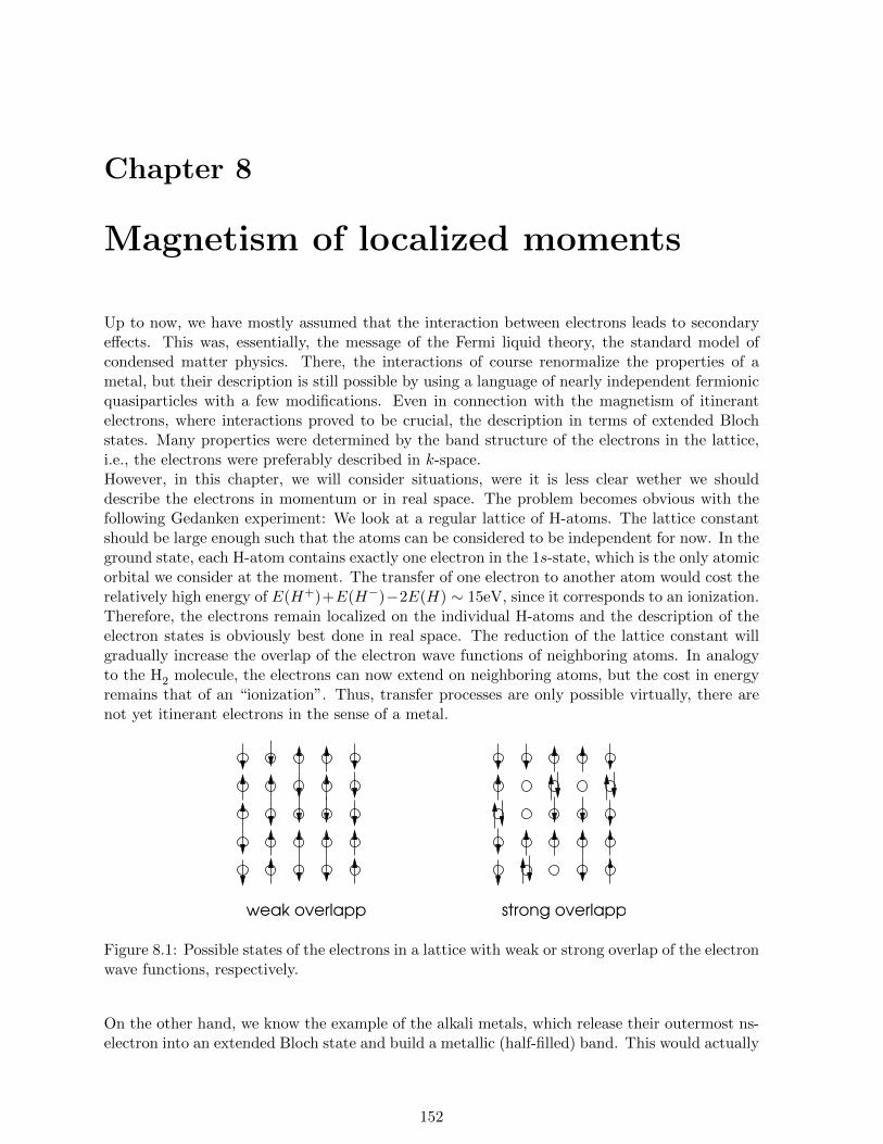
Chapter 8

Magnetism of localized moments

Up to now, we have mostly assumed that the interaction between electrons leads to secondaryeffects. This was, essentially, the message of the Fermi liquid theory, the standard model ofcondensed matter physics. There, the interactions of course renormalize the properties of ametal, but their description is still possible by using a language of nearly independent fermionicquasiparticles with a few modifications. Even in connection with the magnetism of itinerantelectrons, where interactions proved to be crucial, the description in terms of extended Blochstates. Many properties were determined by the band structure of the electrons in the lattice,i.e., the electrons were preferably described in k-space.However, in this chapter, we will consider situations, were it is less clear wether we shoulddescribe the electrons in momentum or in real space. The problem becomes obvious with thefollowing Gedanken experiment: We look at a regular lattice of H-atoms. The lattice constantshould be large enough such that the atoms can be considered to be independent for now. In theground state, each H-atom contains exactly one electron in the 1s-state, which is the only atomicorbital we consider at the moment. The transfer of one electron to another atom would cost therelatively high energy of E(H+)+E(H−)−2E(H) ∼ 15eV, since it corresponds to an ionization.Therefore, the electrons remain localized on the individual H-atoms and the description of theelectron states is obviously best done in real space. The reduction of the lattice constant willgradually increase the overlap of the electron wave functions of neighboring atoms. In analogyto the H2 molecule, the electrons can now extend on neighboring atoms, but the cost in energyremains that of an “ionization”. Thus, transfer processes are only possible virtually, there arenot yet itinerant electrons in the sense of a metal.

strong overlappweak overlapp

Figure 8.1: Possible states of the electrons in a lattice with weak or strong overlap of the electronwave functions, respectively.

On the other hand, we know the example of the alkali metals, which release their outermost ns-electron into an extended Bloch state and build a metallic (half-filled) band. This would actually

152

work well for the H-atoms for sufficiently small lattice constant too.1 Obviously, a transitionbetween the two limiting behaviors should exist. This metal-insulator transition, which occurs,if the gain of kinetic energy surpasses the energy costs for the charge transfer. The insulatingside is known as a Mott insulator.While the obviously metallic state is reliably described by the band picture and can be sufficientlywell approximated by the previously discussed methods, this point of view becomes obsoletewhen approaching the metal-insulator transition. According to band theory, a half-filled bandmust produce a metal, which definitely turns wrong when entering the insulating side of thetransition. Unfortunately, no well controlled approximation for the description of this metal-insulator transition exists, since there are no small parameters for a perturbation theory.Another important aspect is the fact, that in a standard Mott insulator each atom featuresan electron in the outermost occupied orbital and, hence, a degree of freedom in the form ofa localized spin s = 1/2, in the simplest case. While charge degrees of freedom (motion ofelectrons) are frozen at small temperatures, the same does not apply to these spin degrees offreedom. Many interesting magnetic phenomena are produced by the coupling of these spins.Other, more general forms of Mott insulators exist as well, which include more complex formsof localized degrees of freedom, e.g., partially occupied degenerate orbital states.

8.1 Mott transition

First, we investigate the metal-insulator transition. Its description is difficult, since it doesnot constitute a transition between an ordered and a disordered state in the usual sense. Wewill, however, use some simple considerations which will allow us to gain some insight into thebehavior of such systems.

8.1.1 Hubbard model

We introduce a model, which is based on the tight-binding approximation we have introduced inchapter 1. It is inevitable to go back to a description based on a lattice and give up continuity.The model describes the motion of electrons, if their wave functions on neighboring lattice sitesonly weakly overlap. Furthermore, the Coulomb repulsion, leading to an increase in energy, if asite is doubly occupied, is taken into account. We include this with the lattice analogue of thecontact interaction. The model, called Hubbard model, has the form

H = −t∑〈i,j〉,s

(c†iscjs + h.c.) + U∑i

ni↑ni↓, (8.1)

where we consider hopping between nearest neighbors only, via the matrix element −t. Note,

that c(†)is are real-space field operators on the lattice (site index i) and nis = c†iscis is the density

operator. We focus on half filling, n = 1, one electron per site on average. There are two obviouslimiting cases:

• Insulating atomic limit: We put t = 0. The ground state has exactly one electron oneach lattice site. This state is, however, highly degenerate. In fact, the degeneracy is 2N

(number of sites N), since each electron has spin 1/2, i.e.,

|ΦA0si〉 =∏i

c†i,si |0〉, (8.2)

where the spin configuration si can be chosen arbitrarily. We will deal with the liftingof this degeneracy later. The first excited states feature one lattice site without electron

1In nature, this can only be induced by enormous pressures metallic hydrogen probably exists in the centersof the large gas planets Jupiter and Saturn due to the gravitational pressure.

153

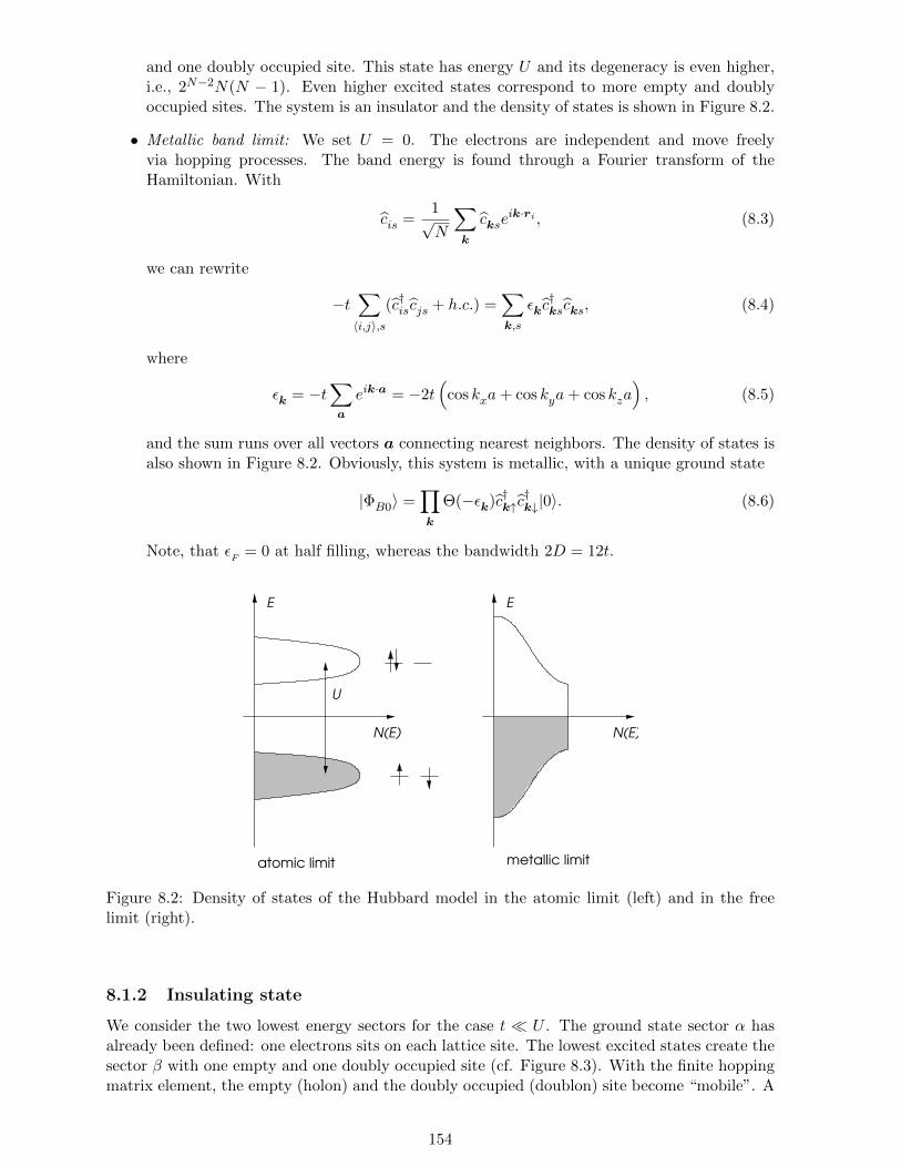
and one doubly occupied site. This state has energy U and its degeneracy is even higher,i.e., 2N−2N(N − 1). Even higher excited states correspond to more empty and doublyoccupied sites. The system is an insulator and the density of states is shown in Figure 8.2.

• Metallic band limit: We set U = 0. The electrons are independent and move freelyvia hopping processes. The band energy is found through a Fourier transform of theHamiltonian. With

cis =1√N

∑k

ckseik·ri , (8.3)

we can rewrite

−t∑〈i,j〉,s

(c†iscjs + h.c.) =∑k,s

εkc†kscks, (8.4)

where

εk = −t∑a

eik·a = −2t(

cos kxa+ cos kya+ cos kza), (8.5)

and the sum runs over all vectors a connecting nearest neighbors. The density of states isalso shown in Figure 8.2. Obviously, this system is metallic, with a unique ground state

|ΦB0〉 =∏k

Θ(−εk)c†k↑c†k↓|0〉. (8.6)

Note, that εF

= 0 at half filling, whereas the bandwidth 2D = 12t.

atomic limit metallic limit

E

N(E) N(E)

E

U

Figure 8.2: Density of states of the Hubbard model in the atomic limit (left) and in the freelimit (right).

8.1.2 Insulating state

We consider the two lowest energy sectors for the case t U . The ground state sector α hasalready been defined: one electrons sits on each lattice site. The lowest excited states create thesector β with one empty and one doubly occupied site (cf. Figure 8.3). With the finite hoppingmatrix element, the empty (holon) and the doubly occupied (doublon) site become “mobile”. A

154

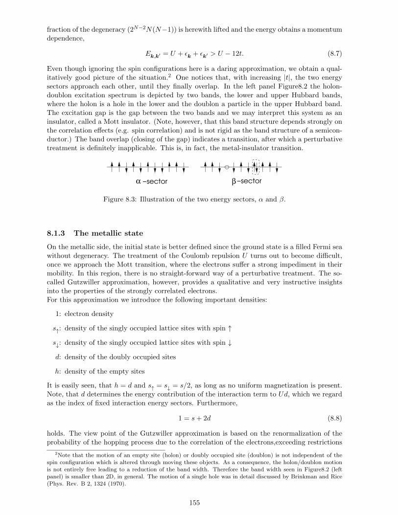
fraction of the degeneracy (2N−2N(N−1)) is herewith lifted and the energy obtains a momentumdependence,

Ek,k′ = U + εk + εk′ > U − 12t. (8.7)

Even though ignoring the spin configurations here is a daring approximation, we obtain a qual-itatively good picture of the situation.2 One notices that, with increasing |t|, the two energysectors approach each other, until they finally overlap. In the left panel Figure8.2 the holon-doublon excitation spectrum is depicted by two bands, the lower and upper Hubbard bands,where the holon is a hole in the lower and the doublon a particle in the upper Hubbard band.The excitation gap is the gap between the two bands and we may interpret this system as aninsulator, called a Mott insulator. (Note, however, that this band structure depends strongly onthe correlation effects (e.g. spin correlation) and is not rigid as the band structure of a semicon-ductor.) The band overlap (closing of the gap) indicates a transition, after which a perturbativetreatment is definitely inapplicable. This is, in fact, the metal-insulator transition.

−sectorα β−sector

Figure 8.3: Illustration of the two energy sectors, α and β.

8.1.3 The metallic state

On the metallic side, the initial state is better defined since the ground state is a filled Fermi seawithout degeneracy. The treatment of the Coulomb repulsion U turns out to become difficult,once we approach the Mott transition, where the electrons suffer a strong impediment in theirmobility. In this region, there is no straight-forward way of a perturbative treatment. The so-called Gutzwiller approximation, however, provides a qualitative and very instructive insightsinto the properties of the strongly correlated electrons.For this approximation we introduce the following important densities:

1: electron density

s↑: density of the singly occupied lattice sites with spin ↑

s↓: density of the singly occupied lattice sites with spin ↓

d: density of the doubly occupied sites

h: density of the empty sites

It is easily seen, that h = d and s↑ = s↓ = s/2, as long as no uniform magnetization is present.Note, that d determines the energy contribution of the interaction term to Ud, which we regardas the index of fixed interaction energy sectors. Furthermore,

1 = s+ 2d (8.8)

holds. The view point of the Gutzwiller approximation is based on the renormalization of theprobability of the hopping process due to the correlation of the electrons,exceeding restrictions

2Note that the motion of an empty site (holon) or doubly occupied site (doublon) is not independent of thespin configuration which is altered through moving these objects. As a consequence, the holon/doublon motionis not entirely free leading to a reduction of the band width. Therefore the band width seen in Figure8.2 (leftpanel) is smaller than 2D, in general. The motion of a single hole was in detail discussed by Brinkman and Rice(Phys. Rev. B 2, 1324 (1970).

155

due to the Pauli principle. With this, the importance of the spatial configuration of the electronsis enhanced. In the Gutzwiller approximation, the latter is taken into account statistically bysimple probabilities for the occupation of lattice sites.We fix the density of the doubly occupied sites d and investigate the hopping processes whichkeep d constant. First, we consider an electron hopping from a singly occupied to an emptysite (i → j). Hopping probability depends on the availability of the initial configuration. Wecompare the probability to find this initial state for the correlated (P ) and the uncorrelated (P0)case and write

P (↑ 0) + P (↓ 0) = gt[P0(↑ 0) + P0(↓ 0)]. (8.9)

The factor gt will eventually appear as the renormalization of the hopping probability and, thus,leads to an effective kinetic energy of the system due to correlations. We determine both sidesstatistically. In the correlated case, the joint probability for i to be singly occupied and j to beempty is obviously

P (↑ 0) + P (↓ 0) = sh = sd = d(1− 2d). (8.10)

where we used equation (8.8). In the uncorrelated case (where d is not fixed), we have

P0(↑ 0) = ni↑(1− ni↓)(1− nj↑)(1− nj↓) =1

16. (8.11)

The case for ↓ follows accordingly. In order to collect the total result for hopping processes whichkeep d constant, we have to do the same calculation for the hopping process (↑↓, ↑) → (↑, ↑↓),which leads to the same result. Processes of the kind (↑↓, 0) → (↑, ↓) leave the sector of fixedd and are ignored.3 With this, we obtain in all cases the same renormalization factor for thekinetic energy,

gt = 8d(1− 2d), (8.12)

i.e., t → gtt. We consider the correlations by treating the electrons as independent but with arenormalized matrix element gtt. The energy in the sector d becomes

E(d) = gtεkin + Ud = 8d(1− 2d)εkin + Ud, εkin =1

N

0∫−D

dε N(ε)ε. (8.13)

For fixed U and t, we can minimize this with respect to d (note that this in not a variationalcalculation in a strict sense, the resulting energy is not an upper bound to the ground stateenergy), and find

d =1

4

(1− U

Uc

)and gt = 1−

(U

Uc

)2

, (8.14)

with the critical value

Uc = 8|εkin| ≈ 25t ∼ 4D. (8.15)

For u ≥ Uc, double occupancy and, thus, hopping is completely suppressed, i.e., electronsbecome localized. This observation by Brinkman and Rice [Phys. Rev. B 2, 4302 (1970)]provides a qualitative description of the metal-insulator transition to a Mott insulator, but

3This formulation is based on plausible arguments. A more rigorous derivation can be found in theliterature, e.g., in D. Vollhardt, Rev. Mod. Phys. 56, 99 (1984); T. Ogawa et al., Prog. Theor.Phys. 53, 614 (1975); S. Huber, Gutzwiller-Approximation to the Hubbard-Model (Proseminar SS02,http://www.itp.phys.ethz.ch/proseminar/condmat02).

156

takes into account only local correlations, while correlations between different lattice sites are notconsidered. Moreover, correlations between the spin degrees of freedom are entirely neglected.The charge excitations contain contributions between different energy scales: (1) a metallic part,described via the renormalized effective Hamiltonian

Hren =∑k,s

gtεkc†kscks + Ud, (8.16)

and (2) a part with higher energy, corresponding to charge excitations on the energy scale U ,i.e., to excitations raising the number of doubly occupied sites by one (or more).We can estimate the contribution to the metallic conduction. Since in the tight-binding descrip-tion the current operator contains the hopping matrix element and is thus subject to the samerenormalization as the kinetic energy, we obtain

σ1(ω) =ω∗2p4δ(ω) + σhigh energy

1 (ω), (8.17)

where we have used equation (6.12) for a perfect conductor (no residual resistivity in a perfectlattice). There is a high-energy part which we do not specify here. The plasma frequency isrenormalized, ω∗2p = gtω

2p, such that the f -sum rule in equation (6.13) yields

I =

∞∫0

dωσ1(ω) =ω2p

8gt + Ihigh energy =

ω2p

8. (8.18)

For U → Uc, the coherent metallic part becomes weaker and weaker,

ω2p

8gt =

(1−

(U

Uc

)2)ω2p

8. (8.19)

According to the f -sum rule, the lost weight must gradually be transferred to the “high-energy”contribution.

8.1.4 Fermi liquid properties of the metallic state

The just discussed approximation allows us to discuss a few Fermi liquid properties of the metallicstate close to metal-insulator transition in a simplified way. Let us investigate the momentumdistribution. According to the above definition,

εkin =1

N

∑k∈FS

εk, (8.20)

where the sum runs over all k in the Fermi sea (FS). One can show within the above approxi-mation, that the distribution is a constant within (nin) and outside (nout) the Fermi surface forfinite U , such that, for k in the first Brillouin zone,

1

2=

1

N

∑k∈FS

nin +1

N

∑k/∈FS

nout =1

2(nin + nout) (8.21)

and

gtεkin =1

N

∑k∈FS

ninεk +1

N

∑k/∈FS

noutεk. (8.22)

Taking into account particle-hole symmetry, i.e.,∑k

εk =∑k∈FS

εk +∑k/∈FS

εk = 0, (8.23)

157

we are able to determine nin and nout,

nin + nout = 1

nin − nout = gt

⇒

nin = (1 + gt)/2

nout = (1− gt)/2. (8.24)

With this, the jump in the distribution at the Fermi energy is equal to gt, which, as previously,corresponds to the quasiparticle weight (cf. Figure 8.4). For U → Uc it vanihes, i.e., thequasiparticles cease to exist for U = Uc.

kF

nk

gt

k

Figure 8.4: The distribution function in the Gutzwiller approximation, displaying the jump atthe Fermi energy.

Without going into the details of the calculation, we provide a few Fermi liquid parameters. Itis easy to see that the effective mass

m

m∗= gt, (8.25)

and thus

F s1 = 3(g−1t − 1

)=

3U2

U2c − U2

, (8.26)

where t = 1/2m and the density of states N(εF

)∗ = N(εF

)g−1t . Furthermore,

F a0 = −UN(εF

)

4

2Uc + U

(U + Uc)2Uc, ⇒ χ =

µ2BN(ε

F)∗

1 + F a0, (8.27)

F s0 =UN(ε

F)

4

2UC− U

(U − Uc)2Uc, ⇒ κ =

N(εF

)∗

n2(1 + F s0 ). (8.28)

It follows, that the compressibility κ vanishes for U → Uc as expected, since it becomes more andmore difficult to compress the electrons or to add more electrons, respectively. The insulator is, ofcurse, incompressible. The spin susceptibility diverges because of the diverging density of statesN(ε

F)∗. This indicates, that local spins form, which exist as completely independent degrees of

freedom at U = Uc. Only the antiferromagnetic correlation between the spins would lead to arenormalization, which turns χ finite. This correlation is, as mentioned above, neglected in theGutzwiller approximation. The effective mass diverges and shows that the quasiparticles aremore and more localized close to the transition, since the occupation of a lattice site is gettingmore rigidly fixed to 1.4 As a last remark, it turns out that the Gutzwiller approximation iswell suited to describe the strongly correlated Fermi liquid 3He (cf. [D. Vollhardt, Rev. Mod.Phys. 56, 99 (1984)]).

4This can be observed within the Gutzwiller approximation in the form of local fluctuations of the particlenumber. For this, we introduce the density matrix of the electron states on an arbitrary lattice site,

ρ = h|0〉〈0|+ d|↑↓〉〈↑↓|+ s

2(|↑〉〈↑|+ |↓〉〈↓|) , (8.29)

158

8.2 The Mott insulator as a quantum spin system

One of the most important characteristics of the Mott insulator is the presence of spin degrees offreedom after the freezing of the charge. This is one of the most profound features distinguishinga Mott insulator from a band insulator. In our simple discussion, we have seen that the atomiclimit of the Mott insulator provides us with a highly degenerate ground state, where a spin-1/2degree of freedom is present on each lattice site. We lift this degeneracy by taking into accountthe kinetic energy term Hkin (t U). In this way new physics appears on a low-energy scale,which can be described by an effective spin Hamiltonian. Prominent examples for such spinsystems are transition-metal oxides like the cuprates La2CuO4, SrCu2O3 or vanadates CaV4O9,NaV2O5.

8.2.1 The effective Hamiltonian

In order to employ our perturbative considerations, it is sufficient to observe the spins of twoneighboring lattice sites and to consider perturbation theory for discrete degenerate states. Here,this is preferably done in real space. There are 4 degenerate configurations, | ↑, ↑〉, | ↑, ↓〉, | ↓, ↑〉, | ↓, ↓〉. The application of Hkin yields

Hkin| ↑, ↑〉 = Hkin| ↓, ↓〉 = 0, (8.31)

Hkin| ↑, ↓〉 = −Hkin| ↓, ↑〉 = −t| ↑↓, 0〉 − t|0, ↑↓〉, (8.32)

where, in the last two cases, the resulting states have an energy higher by U and lie outside theground state sector. Thus, it becomes clear that we have to proceed to second order perturbation,where the states of higher energy will appear only virtually (cf. Figure 8.5).

or−t −t

E = U

virtual states

initial final

spin configurationsspin configuration

Figure 8.5: Illustration of the origin of the superexchange.

We obtain the matrix elements

Ms1,s2;s′1,s′2

= −∑n

〈s1, s2|Hkin|n〉1

〈n|HCoul|n〉〈n|Hkin|s′1, s′′2〉, (8.33)

where |n〉 = | ↑↓, 0〉 or |0, ↑↓〉, such that the denominator is always U . We end up with

M↑↓;↑↓ = M↓↑;↓↑ = −M↑↓;↓↑ = −M↓↑;↑↓ = −2t2

U. (8.34)

from which we deduce the variance of the occupation number,

〈n2〉 − 〈n〉2 = 〈n2〉 − 1 = tr(ρn2)− 1 = 4d+ s− 1 = 2d. (8.30)

The deviation from single occupation vanishes with d, i.e., with the approach of the metal-insulator transition.Note that the dissipation-fluctuation theorem connects 〈n2〉 − 〈n〉2 to the compressibility.

159

Note that the signs originates from the anti-commutation properties of the Fermion operators.In the subspace | ↑, ↓〉, | ↓, ↑〉 we find the eigenstates of the respective secular equations,

1√2

(| ↑, ↓〉+ | ↓, ↑〉) , E = 0, (8.35)

1√2

(| ↑, ↓〉 − | ↓, ↑〉) , E = −4t2

U. (8.36)

Since the states | ↑, ↑〉 and | ↓, ↓〉 have energy E = 0, the sector with total spin S = 1 isdegenerate (spin triplet). The spin sector S = 0 with the energy −4t2/U is the ground state(spin singlet).An effective Hamiltonian with the same energy spectrum for the spin configurations can bewritten with the help of the spin operators S1 and S2 on the two lattice sites

Heff = J

(S1 · S2 −

~2

4

), J =

4t2

U~2> 0. (8.37)

This mechanism of spin-spin coupling is called superexchange and introduced by P.W. Anderson[Phys. Rev. 79, 350 (1950)].Since this relation is valid between all neighboring lattice sites, we can write the total Hamilto-nian as

HH

= J∑〈i,j〉

Si · Sj + const. (8.38)

This model, reduced to spins only, is called Heisenberg model. The Hamiltonian is invariantunder a global SU(2) spin rotation,

Us(θ) = e−iS·θ, S =∑j

Sj . (8.39)

Thus, the total spin is a good quantum number, as we have seen in the two-spin case. Thecoupling constant is positive and favors an antiparallel alignment of neighboring spins. Theground state is therefore not ferromagnetic.

8.2.2 Mean field approximation of the anti-ferromagnet

There are a few exact results for the Heisenberg model, but not even the ground state energycan be calculated exactly (except in the case of the one-dimensional spin chain which can besolved by means of a Bethe Ansatz). The difficulty lies predominantly in the treatment ofquantum fluctuations, i.e., the zero-point motion of coupled spins. It is easiest seen alreadywith two spins, where the ground state is a singlet and maximally entangled. The ground stateof all antiferromagnetic systems is a spin singlet (Stot = 0). In the so-called thermodynamiclimit (N →∞) there is long-ranged anti-ferromagnetic order in the ground state for dimensionsD ≥ 2. Contrarily, the fully polarized ferromagnetic state (ground state for a model with J < 0)is known exactly, and as a state with maximal spin quantum number S2 it features no quantumfluctuations.In order to describe the antiferromagnetic state anyway, we apply the mean field approximationagain. We can characterize the equilibrium state of the classical Heisenberg model (spins assimple vectors without quantum properties) by splitting the lattice into two sublattices A andB, where each A-site has only B-sites as neighbors, and vice-versa.5 On the A-(B-)sublattice,the spins point up (down). This is unique up to a global spin rotations. Note, that this spin

5Lattices which allow for such a separation are called bipartite. There are lattices, where this is not possible,e.g., triangular or cubic face centered lattices. There, frustration phenomena appear, a further complication ofanti-ferromagnetically coupled systems.

160

configuration doubles the unit cell.We introduce the respective mean field,

Szi =

m+ (Szi −m) i ∈ A

−m+ (Szi +m) i ∈ B. (8.40)

This leads to the mean field Hamiltonian

Hmf = HA

+HB

= −Jzm∑i∈A

Szi + Jzm∑i∈B

Szi + Jzm2

2N + · · · , (8.41)

with the coordination number z, the number of nearest neighbors (z = 6 in a simple cubiclattice). It is simple to calculate the partition sum of this Hamiltonian,

Z = tr(e−βHmf

)=[(eβJmz~/2 + e−βJmz~/2

)e−βJzm

2/2]N

. (8.42)

The free energy per spin is consequently given by

F (m,T ) = − 1

NkBT lnZ = Jz

m2

2− k

BT ln (2 cosh(βJzm~/2)) . (8.43)

At fixed temperature, we minimize the free energy with respect to m to determine the thermalequilibrium state,6 i.e., set ∂F/∂m = 0 and find

m =~2

tanh

(Jzm~2k

BT

). (8.44)

This is the self-consistency equation of the mean field theory. It provides a critical temperatureTN

(Neel temperature), below which the mean moment m is finite. For T → TN−, m approaches0 continuously. Thus, T

Ncan be found from a linearized self-consistency equation,

m =Jzm~2

4kBT

∣∣∣∣T=TN

, (8.45)

and thus

TN

=Jz~2

4kB

. (8.46)

This means, that TN

scales with the coupling constant and with z. The larger J and the moreneighbors are present, the more stable is the ordered state.7 For T close to T

N, we can expand

the free energy in m,

F (m,T ) = F0 +Jz

2

[(1− T

N

T

)m2 +

2

3~2

(TN

T

)3

m4 · · ·]. (8.47)

This is a Landau theory for a phase transition of second order, where a symmetry is spon-taneously broken. The breaking of the symmetry (from the high-temperature phase with highsymmetry to the low-temperature phase with low symmetry) is described by the order parameterm. The minimization of F with respect to m yields (cf. Figure 8.6)

m(T ) =

0, T > T

N,

~2

√3(T

N/T − 1), T ≤ T

N.

(8.48)

6Actually, a magnetic field pointing into the opposite direction on each site would be another equilibriumvariable (next to the temperature). We set it to zero.

7At infinite z, the mean field approximation becomes exact.

161

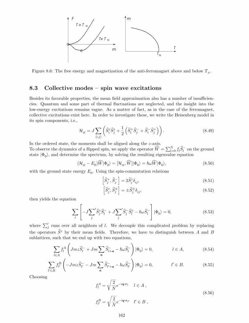
m

T

m

T

T< T N

T > T N

F

N

Figure 8.6: The free energy and magnetization of the anti-ferromagnet above and below TN.

8.3 Collective modes – spin wave excitations

Besides its favorable properties, the mean field approximation also has a number of insufficien-cies. Quantum and some part of thermal fluctuations are neglected, and the insight into thelow-energy excitations remains vague. As a matter of fact, as in the case of the ferromagnet,collective excitations exist here. In order to investigate these, we write the Heisenberg model inits spin components, i.e.,

HH

= J∑〈i,j〉

(Szi S

zj +

1

2

(S+i S−j + S−i S

+j

)). (8.49)

In the ordered state, the moments shall be aligned along the z-axis.To observe the dynamics of a flipped spin, we apply the operator W =

∑Nl=0 flS

−l on the ground

state |Φ0〉, and determine the spectrum, by solving the resulting eigenvalue equation

(HH− E0)W |Φ0〉 = [H

H, W ]|Φ0〉 = ~ωW |Φ0〉, (8.50)

with the ground state energy E0. Using the spin-commutation relations[S+j , S

−j

]= 2Szj δij , (8.51)[

Szj , S±j

]= ±S±j δij , (8.52)

then yields the equation

∑l

−J∑j

′Szj S

−l + J

∑j

′S−j S

zl − ~ωS−l

|Φ0〉 = 0, (8.53)

where∑′

j runs over all neighbors of l. We decouple this complicated problem by replacing

the operators Sz by their mean fields. Therefore, we have to distinguish between A and Bsublattices, such that we end up with two equations,∑

l∈AfAl

(JmzS−l + Jm

∑a

S−l+a − ~ωS−l

)|Φ0〉 = 0, l ∈ A, (8.54)

∑l′∈B

fBl′

(−JmzS−l′ − Jm

∑a

S−l′+a − ~ωS−l′

)|Φ0〉 = 0, l′ ∈ B. (8.55)

Choosing

fAl =

√2

Ne−iq·rl l ∈ A ,

fBl′ =

√2

Ne−iq·rl′ l′ ∈ B ,

(8.56)

162

we introduce the operators

S−l =

√2

N

∑q

a†qeiq·rl , (8.57)

S−l′ =

√2

N

∑q

b†qeiq·rl′ , (8.58)

with l ∈ A and l′ ∈ B, and, vice versa,

a†q =

√2

N

∑l∈A

S−l e−iq·rl , (8.59)

b†q =

√2

N

∑l′∈B

S−l′ e−iq·rl′ , (8.60)

and insert them into the equation and obtain,((Jmz − ~ω)

∑l∈A

S−l e−iq·rl + Jm

∑a

eiq·a∑l′∈B

S−l′ e−iq·rl′

)|Φ0〉 = 0, (8.61)(

(−Jmz − ~ω)∑l′∈B

S−l′ e−iq·rl′ − Jm

∑a

eiq·a∑l∈A

S−l e−iq·rl

)|Φ0〉 = 0. (8.62)

From this follows that ((Jmz − ~ω)a†q + Jmγq b

†q

)|Φ0〉 = 0, (8.63)(

(−Jmz − ~ω)b†q − Jmγqa†q)|Φ0〉 = 0, (8.64)

with γq =∑a e

iq·a = 2(cos qxa + cos qya + cos qza). This eigenvalue equation is easily solvedleading to the description of spin waves in the antiferromagnet. The energy spectrum is givenby

~ωq = ±Jm√z2 − γ2

q. (8.65)

Note, that only the positive energies make sense. It is interesting to investigate the limit ofsmall q,

z2 − γ2q → z2q2 +O(q4), (8.66)

where

~ωq = Jmz|q|+ · · · . (8.67)

This means that, in contrast to the ferromagnet, the spin waves of the antiferromagnet have alinear low-energy spectrum (cf. Figure 8.7). The same applies here if we expand the spectrumaround Q = (1, 1, 1)π/a (folding of the Brillouin zone due to the doubling of the unit cell).After a suitable normalization, the operators aq and bq are of bosonic nature; this comes about

since, due to the mean field approximation, the S±l are bosonic as well,

[S+l , S

−j ] = 2Szl δlj ≈ ±2mδlj , (8.68)

where the sign depends on the sublattice. The zero-point fluctuations of these bosons yield quan-tum fluctuations, which reduce the moment m from its mean field value. In a one-dimensional

163

q

hωq

π

2a

Bri

llo

uin

zo

ne

bo

un

dar

y o

f re

du

ced

Figure 8.7: Spectrum of the spin waves in the antiferromagnet.

spin chain these fluctuations are strong enough to suppress antiferromagnetically order even forthe ground state. The fact that the spectrum starts at zero has to do with the infinite degener-acy of the ground state. The ordered moments can be turned into any direction globally. Thisproperty is known under the name Goldstone theorem, which tells that each ordered state thatbreaks a continuous symmetry has collective excitations with arbitrary small (positive) energies.The linear spectrum is normal for collective excitations of this kind; the quadratic spectrum ofthe ferromagnet has to do with the fact that the state breaks time-inversion symmetry.These spin excitations show the difference between a band and a Mott insulator very clearly.While in the band insulator both charge and spin excitations have an energy gap and are inert,the Mott insulator has only gapped charge excitation. However, the spin degrees of freedom fora low-energy sector which can even form gapless excitations as shown just above.

164