Solar Sails: Modeling, Estimation, and Trajectory...
164
Solar Sails: Modeling, Estimation, and Trajectory Control by Leonel Rios-Reyes A dissertation submitted in partial fulfillment of the requirements for the degree of Doctor of Philosophy (Aerospace Engineering) in The University of Michigan 2006 Doctoral Committee: Professor Daniel J. Scheeres, Chair Professor N. Harris McClamroch Professor Pierre T. Kabamba Professor Thomas H. Zurbuchen Dr. Michael E. Lisano, Jet Propulsion Laboratory
Transcript of Solar Sails: Modeling, Estimation, and Trajectory...

Solar Sails: Modeling, Estimation, and
Trajectory Control
by
Leonel Rios-Reyes
A dissertation submitted in partial fulfillmentof the requirements for the degree of
Doctor of Philosophy(Aerospace Engineering)
in The University of Michigan2006
Doctoral Committee:
Professor Daniel J. Scheeres, ChairProfessor N. Harris McClamrochProfessor Pierre T. KabambaProfessor Thomas H. ZurbuchenDr. Michael E. Lisano, Jet Propulsion Laboratory


c© Leonel Rios-ReyesAll rights reserved
2006

To my parents
ii

ACKNOWLEDGEMENTS
I want to give special recognition to the support of my family throughout all
these years, especially my dad, Hector, and my mom, Alicia. Also, I want to thank
my sister, Ethel, and brother, Leonardo, for their constant encouragement. Muchas
gracias.
Also, I want thank my doctoral committee members for their comments on this
dissertation. I am grateful with my advisor, Prof. Scheeres, for his guidance on my
research, for his patience, and for given me encouragement.
I also want to express gratitude to all of my professors from elementary school
to now, since each of them contributed in part to my education. Some of them are
Prof. Joseph Katz, Prof. Allen Plotkin, and Prof. John Conly from San Diego Sate
University; Prof. Edgar Rojano, Prof. Horacio Monroy, and Prof. Jose Angel Tovar
from CBTIS 237 in Mexico.
I want to thank my close friends Nalin Chaturvedi, Matthew McNenly, Fu-Yuen
Hsiao, Ryan Park, Stephen Broschart, Fabio Riviera, Amit Sanyal, Angie Krebs,
Dennis Crespo, David Tello, Rosaicela Roman, Chad Berman, Leonel Flores, Rodrigo
Zuniga, Abel Sanchez Tellez, Armando Rodriguez, Luis Fernando Martinez, Luis
Alberto Cueto, Juan Carlos Arredondo, and Moises Aranda for all the fun times.
Special thanks to Margaret Fillion and Denise Phelps.
The work presented in this dissertation was funded in part by the Jet propul-
sion Laboratory, California Institute of Technology which is under contract with the
iii

National Aeronautics and Space Administration.
iv

TABLE OF CONTENTS
DEDICATION . . . . . . . . . . . . . . . . . . . . . . . . . . . . . . . . . . ii
ACKNOWLEDGEMENTS . . . . . . . . . . . . . . . . . . . . . . . . . . iii
LIST OF FIGURES . . . . . . . . . . . . . . . . . . . . . . . . . . . . . . . viii
LIST OF TABLES . . . . . . . . . . . . . . . . . . . . . . . . . . . . . . . . xi
ABSTRACT . . . . . . . . . . . . . . . . . . . . . . . . . . . . . . . . . . . xii
CHAPTER
I. Introduction . . . . . . . . . . . . . . . . . . . . . . . . . . . . . . 1
1.1 Brief History of Solar Sails . . . . . . . . . . . . . . . . . . . 11.2 Thesis Structure . . . . . . . . . . . . . . . . . . . . . . . . . 4
II. Dynamical Model and Flat Sail Models . . . . . . . . . . . . . 9
2.1 Restricted Two-Body Problem . . . . . . . . . . . . . . . . . 92.2 Circular Restricted Three-Body Problem . . . . . . . . . . . . 102.3 Solar Radiation Pressure Model . . . . . . . . . . . . . . . . . 112.4 Flat Solar Sail Models . . . . . . . . . . . . . . . . . . . . . . 13
2.4.1 Ideal Flat Sail Model . . . . . . . . . . . . . . . . . 142.4.2 Non-Ideal Flat Sail Model . . . . . . . . . . . . . . 17
III. Generalized Sail Model . . . . . . . . . . . . . . . . . . . . . . . . 21
3.1 Sail Surface and Normal Vector . . . . . . . . . . . . . . . . . 213.2 Derivation of the Generalized Sail Force Equation . . . . . . . 223.3 Derivation of the Generalized Sail Moment Equation . . . . . 273.4 Center of Pressure . . . . . . . . . . . . . . . . . . . . . . . . 283.5 Properties of the Tensor Coefficients and Symmetric Sails . . 30
3.5.1 Force Tensors . . . . . . . . . . . . . . . . . . . . . 313.5.2 Moment Tensors . . . . . . . . . . . . . . . . . . . . 34
v

IV. Applications of the Generalized Sail Model . . . . . . . . . . . 37
4.1 Solar Sail Models . . . . . . . . . . . . . . . . . . . . . . . . . 374.1.1 Flat Sail . . . . . . . . . . . . . . . . . . . . . . . . 374.1.2 Circular Sail with Billow . . . . . . . . . . . . . . . 384.1.3 Four-Panel Sail with Billow . . . . . . . . . . . . . . 424.1.4 Generic Sail Model . . . . . . . . . . . . . . . . . . 51
4.2 Comparison of Sail Geometries . . . . . . . . . . . . . . . . . 554.3 GSM Partial Derivatives . . . . . . . . . . . . . . . . . . . . . 56
4.3.1 First-Order Partial Derivatives of the Force Equation 584.4 Second-Order Force Partial Derivatives . . . . . . . . . . . . . 614.5 Force Partial Derivatives with respect to Control Angles . . . 624.6 Second Order Force Partial with respect to Control Angles . . 644.7 Locally Optimal Control Laws . . . . . . . . . . . . . . . . . 66
4.7.1 Maximum Energy Increase . . . . . . . . . . . . . . 664.7.2 Maximum Propulsive Force . . . . . . . . . . . . . . 69
4.8 Applications of GSM to NASA’s S5 Project . . . . . . . . . . 71
V. Estimation: Force, Moment, and Optical Parameters . . . . . 75
5.1 Linear Estimation of GSM Tensor Coefficients . . . . . . . . . 765.2 Force and Moment in Linear Form . . . . . . . . . . . . . . . 775.3 Least-Squares Estimation . . . . . . . . . . . . . . . . . . . . 80
5.3.1 Predicted Force and Moment Uncertainty . . . . . . 825.4 Numerical Linear Estimation . . . . . . . . . . . . . . . . . . 83
5.4.1 Force Estimation . . . . . . . . . . . . . . . . . . . 835.4.2 Moment Estimation . . . . . . . . . . . . . . . . . . 91
5.5 Symmetric Sail Shapes . . . . . . . . . . . . . . . . . . . . . . 955.5.1 Force Tensor Coefficients . . . . . . . . . . . . . . . 955.5.2 Moment Tensor Coefficients . . . . . . . . . . . . . 96
5.6 Discussion . . . . . . . . . . . . . . . . . . . . . . . . . . . . 97
VI. Solar Sail Trajectory Control . . . . . . . . . . . . . . . . . . . . 98
6.1 Circular Restricted Three Body Problem in Cylindrical Coor-dinates . . . . . . . . . . . . . . . . . . . . . . . . . . . . . . 101
6.2 Sail Propulsive Model . . . . . . . . . . . . . . . . . . . . . . 1036.3 Special Orbits in the Solar Sail CR3BP . . . . . . . . . . . . 105
6.3.1 Sub-L1 Points . . . . . . . . . . . . . . . . . . . . . 1056.3.2 Halo Orbits about Sub-L1 Points . . . . . . . . . . . 106
6.4 Excess Performance in the Sail Propulsion Unit . . . . . . . . 1076.5 Control of Sail Orbit about a Sub-L1 Point . . . . . . . . . . 111
6.5.1 Control of Sail x-Position . . . . . . . . . . . . . . . 1116.5.2 Control of Sail Orbit Radius . . . . . . . . . . . . . 115
vi

6.6 Control about a Sub-L1 Halo Orbit . . . . . . . . . . . . . . . 1176.7 Sail Propulsive Model Estimation . . . . . . . . . . . . . . . . 1196.8 Sail Control Under Degradation . . . . . . . . . . . . . . . . . 1236.9 Control Implementation . . . . . . . . . . . . . . . . . . . . . 126
VII. Conclusions . . . . . . . . . . . . . . . . . . . . . . . . . . . . . . . 131
7.1 Main Results in this Dissertation . . . . . . . . . . . . . . . . 1327.2 Future Research . . . . . . . . . . . . . . . . . . . . . . . . . 134
APPENDIX . . . . . . . . . . . . . . . . . . . . . . . . . . . . . . . . . . . . 136
BIBLIOGRAPHY . . . . . . . . . . . . . . . . . . . . . . . . . . . . . . . . 147
vii

LIST OF FIGURES
Figure
2.1 Geometry of the Restricted Three Body Problem. . . . . . . . . . . 12
2.2 Ideal Sail Model. . . . . . . . . . . . . . . . . . . . . . . . . . . . . 15
2.3 Sail Control Angles. α is the angle between n and −r, δ is the anglebetween the projection of n into the (e2, e3)-plane and the e2-axis. . 17
2.4 Non-ideal force directions. Frs force reflected specularly, Fe force dueemission, Frd force reflected diffusively, and Fa force due to absorption. 18
3.1 Symmetric sail planforms and axis of symmetry. . . . . . . . . . . . 30
3.2 Projection of sail area into symmetry plane. . . . . . . . . . . . . . 32
4.1 Circular Sail Geometry. . . . . . . . . . . . . . . . . . . . . . . . . . 39
4.2 Square Sail Modeling. . . . . . . . . . . . . . . . . . . . . . . . . . . 43
4.3 Sail Area Modeling. . . . . . . . . . . . . . . . . . . . . . . . . . . . 44
4.4 Cone Radius. . . . . . . . . . . . . . . . . . . . . . . . . . . . . . . 45
4.5 Sinusoid Sail Shape. . . . . . . . . . . . . . . . . . . . . . . . . . . . 53
4.6 Normalized force comparison of different sail geometries. . . . . . . 56
4.7 Normalized moment along the sail body-fixed axes. . . . . . . . . . 57
4.8 Local polar coordinate frame and sail body-fixed frame. . . . . . . . 67
4.9 Trajectories for realistic and ideal guidance laws. . . . . . . . . . . . 69
4.10 Energy increase for realistic and ideal guidance laws. . . . . . . . . 70
viii

4.11 Integration of S5. . . . . . . . . . . . . . . . . . . . . . . . . . . . . 74
5.1 Case I. Projected attitude measurements . . . . . . . . . . . . . . . 84
5.2 Case II. Projected attitude measurements . . . . . . . . . . . . . . . 85
5.3 Case III. Projected attitude measurements . . . . . . . . . . . . . . 85
5.4 Case IV. Projected attitude measurements . . . . . . . . . . . . . . 86
5.5 Case I. Covariance of GSM force coefficients . . . . . . . . . . . . . 86
5.6 Case II. Covariance of GSM force coefficients . . . . . . . . . . . . . 87
5.7 Case III. Covariance of GSM force coefficients . . . . . . . . . . . . 87
5.8 Case IV. Covariance of GSM force coefficients . . . . . . . . . . . . 88
5.9 Case I. Correlation of GSM force coefficients . . . . . . . . . . . . . 88
5.10 Case II. Correlation of GSM force coefficients . . . . . . . . . . . . . 89
5.11 Case III. Correlation of GSM force coefficients . . . . . . . . . . . . 89
5.12 Case IV. Correlation of GSM force coefficients . . . . . . . . . . . . 90
5.13 Force Covariance. . . . . . . . . . . . . . . . . . . . . . . . . . . . . 91
5.14 Representative Force Estimation Results. . . . . . . . . . . . . . . . 92
5.15 Case III. Covariance of GSM moment coefficients. . . . . . . . . . . 92
5.16 Case IV. Covariance of GSM moment coefficients. . . . . . . . . . . 93
5.17 Case III. Correlation of GSM moment coefficients. . . . . . . . . . . 93
5.18 Case IV. Correlation of GSM moment coefficients. . . . . . . . . . . 94
5.19 Representative Moment Estimation Results. . . . . . . . . . . . . . 94
6.1 Sail in Orbit about Sub-L1 Point. . . . . . . . . . . . . . . . . . . . 102
6.2 Long term orbit about sub-L1 point for uncontrolled dynamics. . . . 110
ix

6.3 Linear Feedback Control on Sail x-Position. . . . . . . . . . . . . . . 113
6.4 Active Proportional Derivative Control on Sail x-Position. . . . . . 115
6.5 Energy Controlled Sail. . . . . . . . . . . . . . . . . . . . . . . . . . 117
6.6 Sail about a General Trajectory. . . . . . . . . . . . . . . . . . . . . 119
6.7 Relative sail orbit with respect to moving point on halo orbit. Timeof propagation is 3.65 days. . . . . . . . . . . . . . . . . . . . . . . . 120
6.8 Controlled sail about Halo Orbit about sub-L1 point. . . . . . . . . 120
6.9 Adaptive controller. . . . . . . . . . . . . . . . . . . . . . . . . . . . 123
6.10 Adaptive controller for the simple PD-Controller. . . . . . . . . . . 124
6.11 Solar sail under degradation. . . . . . . . . . . . . . . . . . . . . . . 125
6.12 Solar Sail Under Degradation and Uncertainties. . . . . . . . . . . . 126
6.13 Control moments required for station-keeping SPI sail. . . . . . . . 129
x

LIST OF TABLES
Table
3.1 Simplification of Force Tensor Coefficients due to Symmetry. . . . . 34
3.2 Simplification of Moment Tensor Coefficients due to Symmetry. . . . 36
xi

ABSTRACT
Solar Sails: Modeling, Estimation, and Trajectory Control
by
Leonel Rios-Reyes
Chair: Daniel J. Scheeres
There has been great interest in developing solar sail technology and missions by
several international space agencies in recent years. However, at present there is no
consensus on how one can mathematically model forces and moments acting on a
solar sail. Traditional analytical models and finite element methods are not feasible
for integration into a precise navigation system.
This dissertation takes a step toward resolving this issue by developing tools and
concepts that can be integrated into a precise solar sail navigation system. These
steps are the derivation of a generalized sail model, a linear estimation method for
estimating and predicting forces and moments acting on a solar sail, and a new
trajectory control methodology for tracking a nominal trajectory when the sail per-
formance exceeds the nominal design performance.
The main contributions of this dissertation follow. First, the generalized sail
model (GSM) is defined to analytically describe the forces and moments acting on a
solar sail of arbitrary shape. The GSM is derived by performing an integration, of
all the differential forces and moments acting on the sail, over the sail surface. Next,
xii

the GSM is applied to several examples to illustrate the use of the GSM’s analytic
equations. These examples allow comparisons of forces and moments generated by
different solar sails, the computation of force derivatives, and the application of the
model to orbital mechanics problems. Since it is difficult to model the sail geometry
based on ground measurements, errors in the sail model are expected once the sail is
deployed in space. Due to this difficulty, a least-squares estimation method for the
force and moment coefficients of the GSM is derived. For realistic implementation of
a sail trajectory, the deployed sail must have an excess thrust capacity. We develop
and implement a control methodology for flying a nominal mission profile with such
an excess capacity. Control laws for maintaining a flat, ideal solar sail orbiting an
equilibrium point of the circular restricted three-body problem and tracking neigh-
boring halo orbits are provided. The control laws are tested under several conditions
including solar sail surface degradation.
xiii

CHAPTER I
Introduction
This dissertation makes contributions to solar sail technology. Specifically, it ad-
dresses important issues necessary to successfully navigate a solar sail. These include
solar sail force and moment modeling, force and moment parameter estimation, and
trajectory control. Solar sails use solar radiation pressure to create a propulsive force
in order to achieve a mission. The force created is highly correlated to the sail shape.
In this thesis we provide a model to capture the exact sail geometry and model the
force and moment generated using a set of coefficients. With this analytic result,
the assumption of flat solar sails can be relaxed from mission design and detailed
shape models can be easily represented. This analytic model blends directly to a
methodology to estimate the forces and moments coefficients. Finally, controllers for
maintaining a solar sail on a nominal trajectory are provided.
1.1 Brief History of Solar Sails
The concept of flying solar sails originated in the 20th century. Soon after Maxwell
theoretically proved that radiation produces pressure, people started thinking about
propelling objects using the radiation of the sun [37]. Early in the 1920’s Konstantin
Tsiolkovsky and Fridickh Tsander, both co-workers and Russian engineers, started
1

2
writing about using light to propel ships. The idea of using solar sails for space
navigation originated with Tsander [37].
In the 1950’s the work on solar sails started in the U.S. In the 1970’s NASA
started funding studies on solar sails. In 1976 Jerome L. Wright wrote a paper
showing that it was possible to rendezvous with the comet Halley in 1986 using a
solar sail if launched in 1982 [38]. NASA became interested in this mission called the
Halley Rendezvous Mission. Several studies on solar sails arose from this proposal;
however, the concept was dropped. Later, Wright wrote one of the first books on
solar sails titled “Space Sailing,” which was first published in 1992 [37].
The next milestone in the field of solar sails came from Collin R. McInnes in
1999. He wrote a book titled “Solar Sailing: Technology, Dynamics and Mission
Applications” [21]. The solar sail community regards this book as the reference book
on solar sailing. In this book, McInnes compiled the work available, including his
own, for solar sails at the time.
Several of the world space agencies have also become interested in solar sails. 1n
1999 ESA demonstrated the depolyment of a 20m× 20m sail in a ground test [8]. In
2004 the Japanese Aerospace Exploration Agency, JAXA, successfully deployed two
solar sails onboard a sounding rocket [33]. The sails were composed of four segments
and were clover shaped. NASA performed several tests on sail deployment. In 2004
NASA along with L’Garde engineers demonstrated the deployment of a solar sail
during ground tests [17]; the following year a sail deployment was demonstrated in
vacuum conditions [18].
Despite all this effort, none of the space agencies have specific plans to fly a solar
sail. The first attempt to fly a solar sail came from a private effort by the Planetary
Society, led by Louis Friedman [9]. Cosmos I was built in Russia and launched from a

3
submarine rocket. The first attempt to demonstrate the deployment of Cosmos I was
carried out in July, 2001; however, this attempt was unsuccessful due to a failure in
the rockets. In June 2005, Cosmos I was launched again into space. The mission was
to demonstrate the feasibility of solar sails by raising its orbit using solar radiation
only. A failure in the first stage of the rocket that transported Cosmos I doomed the
mission.
In 2002 NASA funded a project, led by Dr. Michael E. Lisano at JPL, in order
to create a high fidelity tool that would allow the mission design and analysis for
solar sails. This project was completed in 2006. The project is called the Solar Sail
Spaceflight Simulation Software or S5. Several organizations were involved in the
development of S5. These included JPL, The University of Colorado, The University
of Michigan, Ball Aerospace and L’Garde Inc. S5 is composed of several modules
that can be used to study all the aspects of a solar sail mission [7].
Currently there are several researchers that focus on aspects that would allow a
solar sail mission to be successful. L’Garde Inc. [17, 18, 6] and AEC Able [25] are
solar sail manufactures in the U. S. Prof. Bong Wie, at Arizona Sate University, has
performed extensive studies on solar sail attitude control [34, 35]. Dr. Dachwald, at
the German Aerospace Agency (DLR), has performed research on trajectory opti-
mization [3, 2]. Prof. Dale Lawrence, at the University of Colorado, has worked on
solar sail trajectory control [15].
All the previous studies on solar sails were performed using a flat sail model. In
order to study sails with billow, or curvature in its surface, finite element models
are required. However, these model introduce difficulties as they provide forces and
moments computed at specific sail attitudes; hence, it is necessary to interpolate
between these attitudes.

4
Among the contributions made in this thesis, a new methodology is presented to
model analytically solar sails of arbitrary shape. The Generalized Sail Model allows
us to model solar sails using billow with a series of tensors coefficients. This model
is employed in the Solar Radiation Pressure Module of S5.
1.2 Thesis Structure
In Chapter II, the dynamics and equations of motion used throughout this disser-
tation are briefly discussed. First, in section 2.1 the Two-Body problem is reviewed
and some comments are provided. Section 2.2 describes the Circular Restricted
Three-Body Problem and the equations of motion are stated. Also, the models for
solar radiation pressure are given in Section 2.3. The model for the sun as a point
source and as a finite disc are explained. Finally, the traditional flat sail models
are derived in Section 4.1.1. The assumptions on the ideal flat sail model are ex-
plained in Section 2.4.1. Section 2.4.2 explains how deviations from ideal reflection
are captured with the non-ideal flat sail model.
The main contributions of this dissertation build upon the concepts presented
in Chapter II to create an analytic generalized sail model, GSM, for modeling solar
sails of arbitrary shape, a least-squares estimation algorithm based on force and
moment measurements for refinement of the sail model, and a control methodology
for tracking a nominal trajectory for sails with performance in excess of the mission
requirements. The details of these contributions are presented in Chapters III-VI.
In Chapter III the non-ideal flat sail model is used in order to derive a more precise
solar sail model: the generalized sail model. First, it is shown that the differential
equations for the force and moment acting on a solar sail can be written in a form
where the integration of these equations is not independent of sail attitude. Section

5
3.2 provides a derivation of the force equation for solar sails of arbitrary shapes.
Section 3.3 gives an analytic equation for the moment acting on a solar sail due to
its billow. Knowing the force and the moment, it is possible to calculate the sail’s
center of pressure as shown in section 3.4. In Section 3.5 properties of the generalized
sail model tensors are provided. Section 3.5.1 deals specifically with the force tensor
coefficients as well as the simplifications that arise when the sail has symmetries.
Properties of the moment tensor coefficients as well as simplifications due to sail
symmetry are discussed in Section 3.5.2. One conference [29] paper and one journal
[27] paper were published from this chapter.
Chapter IV provides applications of the generalized sail model to a number of
different examples. In Section 4.1 several sail geometries are studied by computing
their force and moment tensors. Section 4.1.1 describes the traditional sail model
and recovers the classical flat sail model equation. In Section 4.1.2 a circular sail
with billow is studied. The force and moment coefficients are computed analytically.
Section 4.1.3 describes the geometry of a square billowed sail. This design is a
good approximation to a L’Garde sail and has been constructed and used in mission
design examples [17]. In Section 4.1.4 the principles for modeling sails using finite
element methods are discussed. This concept is applied to a sinusoid sail with no
symmetries by computing its force and moment tensor coefficients. Given the force
and moment coefficients for all these sail geometries, their resulting force and moment
are compared for several sail attitudes in Section 4.2. In Section 4.3 the GSM force
partial derivatives with respect to the sail attitude, optical parameters and control
angles are derived. First, the partial derivatives needed throughout the rest of the
sections are presented. Section 4.3.1 presents the force partial derivatives with respect
to the sail attitude and each of the optical parameters. In Section 4.4 the force second

6
order partial derivatives are presented with respect to the optical parameters and
sail attitude. The first and second order partial derivatives with respect to the sail
control angles are given in Sections 4.5 and 4.6, respectively. Finally in Section 4.7
the generalized sail model, applied to the four-quadrant billowed sail, as well as the
force partial derivatives are employed to revisit classical orbital mechanics problems
where the flat solar sail had been used before. Specifically, Section 4.7.1 discusses a
guidance law to optimally increase the sail orbit semi-major axis in order to escape
from the solar system. The result is compared with the classical solution for a flat
solar sail. In section 4.7.2, the attitude that provides the maximum force for a single
quadrant of the four-quadrant billow sail is derived. Two conference [26, 31] papers
were presented from this chapter.
Chapter V provides a methodology for refining the sail force and moment models
from test data or measured navigation data. The GSM force and moment equations
are linear with respect to the GSM tensor coefficients; thus a least-squares estima-
tion method is developed. In Section 5.1 the normalized equations for the force and
moments are discussed. In Section 5.2 the force and moment equations are manipu-
lated and presented in linear form, as a product of a matrix, which contains the sail
attitude information, and a vector, which contain the force or moment tensor coef-
ficients to facilitate the estimation. The least-squares algorithm for estimating the
force and moment tensor coefficients is derived in Section 5.3. Section 5.3.1 provides
the covariance for the estimated force and moment based on uncertainties from the
measurements used to perform the estimation. In Section 5.4 the normalized force
and moment data are generated using the sinusoid sail shape in order to simulate
navigation data to test the estimation algorithm. The force estimation results are
presented in Section 5.4.1. Four different attitude sampling cases are used for the
7
force estimation and their results are compared. Section 5.4.2 provides the estimation
results for the moment using two different sampling strategies. Section 5.5 is focused
on the simplification that occurs for sails that present different types of symmetries.
Section 5.5.1 presents the simplified equations for the force estimation, while in Sec-
tion 5.5.2 the simplified moment equation is stated. One conference paper has been
presented from this chapter [30] and a journal paper is under review.
Chapter VI provides control laws for station-keeping an ideal flat sail about a
sub-L1 point and tracking a neighboring halo orbit. In Section 6.1 the equations of
motion for the circular restricted three-body are transformed into polar coordinates
to facilitate the design of control laws. In Section 6.2 the sail acceleration is provided
in the new polar frame. Section 6.3 provides a brief description on the effects of the
solar radiation pressure in the equations of motion and how new equilibria and fam-
ilies of halo orbits arise. This sub-L1 points and corresponding halo orbits are used
as references to stabilized a sail. Section 6.3.1 describes how the sub-L1 points are
dependent on the sail characteristics, how to find them, and their inherent instability
is explained. Section 6.3.2 provides an explanation on how to find the families of
halo orbits about these new equilibrium points. In Section 6.4 the problem of having
a solar sail with a performance greater than the mission requirements is discussed.
In Section 6.5 control laws are presented to stabilize a solar sail about a given sub-L1
point. Two independent controllers are necessary to stabilize the sail distance from
the sun and the orbit radius about the sub-L1 point. Section 6.5.1 provides several
controller for maintaining the sailcraft distance from the sun at the required sub-L1
location. Two proportional-derivative controllers and one linear-feedback controller
are developed and their performances are discussed. In Section 6.5.2 a controller
for stabilizing a sail about a sub-L1 point is presented. The controller is a feed-

8
back controller based on the sail kinetic energy. In Section 6.6 the controllers are
generalized to track a halo orbit in the vicinity of a sub-L1 point. The proportional-
derivative controller is modified to track the velocity of a moving point in the halo
orbit. Then, the energy based controller is extended to account for the energy of the
moving point. Sections 6.7 and 6.8 present preliminary work on the control of a solar
sail that suffers from surface degradation due to the space environment. A simple
adaptive control technique is presented and tested under several conditions. Finally,
Section 6.9 discusses a way of implementing these controllers with an attitude control
system. The sail rotational dynamics are discussed as well as the torques required
to achieve the required rotational rate for a sail using these control strategies. One
conference paper [28] has been presented from this chapter and a journal paper is
under preparation.
Chapter VII provides a summary of the main contributions of this dissertation
and indicates the topics for future research.

CHAPTER II
Dynamical Model and Flat Sail Models
In this chapter the models for the dynamics and flat solar sail models are pre-
sented. The much studied restricted two body problem and three body problem are
briefly presented. Then, the flat model for solar sails is introduced for both ideal
and non-ideal sails. The ideal flat model assumes perfect reflection with no losses.
The non-ideal flat model includes parameters to account for optical and thermal sail
properties.
2.1 Restricted Two-Body Problem
The two-body problem is the only general problem in astrodynamics with a closed
form solution. The orbiting bodies are treated as two point masses under mutual
gravitational attraction. The more massive body is called the primary and the less
massive one is the secondary and their masses are denoted by m1 and m2, respectively.
The equations of motion are
r = −G(m1 + m2)
|r|3 r, (2.1)
where G is the universal constant of gravitation and r is the position of the secondary
body with respect to the primary. The restricted two-body problem is a simplification
9

10
of the two-body problem, which arises when the mass ratio between the secondary
and the primary bodies tends to zero as in the case of a planet and orbiting satellite.
Thus, the gravitational µ parameter can be defined as µ = m1G and the equations
of motion become
r = − µ
|r|3 r. (2.2)
The solution of this problem is obtained by finding integrals of motions, which
are derived in Reference [11].
For a spacecraft with its own propulsion unit the equations of motion are
r = − µ
|r|3 r + a, (2.3)
where a is the acceleration.
2.2 Circular Restricted Three-Body Problem
The equations of motion for a spacecraft under the influence two massive bodies
in a mutually circular orbit can be written in a rotating frame as:
r + 2Ω× r + Ω× (Ω× r) = a +∇U(r), (2.4)
where r is the spacecraft position vector, Ω is the angular velocity of the rotating
frame, a is an acceleration from a propulsion unit acting on the spacecraft, and U(r)
is the three-body problem gravitational potential given by:
U(r) =1− µ
|r1| +µ
|r2| . (2.5)
11
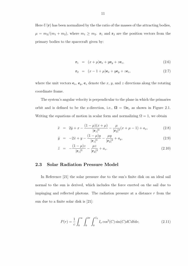
Here U(r) has been normalized by the the ratio of the masses of the attracting bodies,
µ = m2/(m1 + m2), where m1 ≥ m2. r1 and r2 are the position vectors from the
primary bodies to the spacecraft given by:
r1 = (x + µ)ex + yey + zez, (2.6)
r2 = (x− 1 + µ)ex + yey + zez, (2.7)
where the unit vectors ex, ey, ez denote the x, y, and z directions along the rotating
coordinate frame.
The system’s angular velocity is perpendicular to the plane in which the primaries
orbit and is defined to be the z-direction, i.e., Ω = Ωez as shown in Figure 2.1.
Writing the equations of motion in scalar form and normalizing Ω = 1, we obtain
x = 2y + x− (1− µ)(x + µ)
|r1|3 − µ
|r2|3 (x + µ− 1) + ax, (2.8)
y = −2x + y − (1− µ)y
|r1|3 − µy
|r2|3 + ay, (2.9)
z = −(1− µ)z
|r1|3 − µz
|r2|3 + az. (2.10)
2.3 Solar Radiation Pressure Model
In Reference [21] the solar pressure due to the sun’s finite disk on an ideal sail
normal to the sun is derived, which includes the force exerted on the sail due to
impinging and reflected photons. The radiation pressure at a distance r from the
sun due to a finite solar disk is [21]:
P (r) =1
c
∫ ∞
0
∫ 2π
0
∫ C0
0
Iν cos2(C) sin(C)dCdδdν, (2.11)

12
m1
m2
xy
z
r1
r2
S
n
e2
e3e1
Figure 2.1: Geometry of the Restricted Three Body Problem.
where c is the speed of light, C the sun’s apparent angular radius, C0 the maximum
apparent angular radius given by arcsin(Rs/r), Rs is the sun’s radius, r is the distance
from the sun, δ the clock angle, ν the radiation wavelength, and Iν the radiation
specific intensity at a wavelength ν. Since Iν does not depend on r, it can be
averaged over the entire spectrum to yield [21]:
P (r) =2πI0
c
∫ C0
0
cos2(C) sin(C)dC, (2.12)
where I0 is the frequency integrated specific intensity. Performing the integration
and substituting for C0, the radiation pressure becomes [21]:
P (r) =2πI0
3c
1−
[1−
(Rs
r
)2]3/2
. (2.13)
Eq. (2.13) can be rearranged as [21]:
P (r) = P ∗(r)F (r), (2.14)

13
where P ∗(r) is the radiation pressure of a point source given by [21]:
P ∗(r) =I0π
c
(Rs
r
)2
, (2.15)
where I0 = 2.04× 10⁷W/m [21] is the sun’s specific intensity, Rs = 6.96× 10⁸m [11],
and
F (r) =2
3
(r
Rs
)2
1−
[1−
(Rs
r
)2]3/2
. (2.16)
F (r) is a correction function to account for the sun’s finite disk. With this
formalism we assume the solar radiation travels in parallel rays when it reaches the
sail.
The difference between these two models increases with proximity to the sun. As
the distance from the sun increases the difference between the models decreases and
by 10 solar radii the difference is within one percent [21]. Specifically, expanding Eq.
2.19 in powers of (Rs/r) yields
F (r) =2
3
(r
Rs
)2[1− 1 +
3
2
(Rs
r
)2
−O
(Rs
r
)4]
= 1−O
(Rs
r
)2
. (2.17)
2.4 Flat Solar Sail Models
The propulsion on solar sails is generated through the momentum carried by the
solar radiation pressure. When photons strike the sail membrane there is a momen-
tum transfer into the sail as well as when they are reflected. This momentum transfer
is small; by Newton’s second the acceleration and mass are related as a = F/m, there-
fore, in order to generate a useful acceleration, the sailcraft must have a high surface
area to intercept as much as the radiation flux as possible and be lightweight at the

14
same time. The force generated is also dependent on the characteristics of the sail
such as its reflective properties and surface shape. Two widely used sail models for
initial sail studies are the ideal flat model and the non-ideal flat model for solar sails,
which are discussed next.
2.4.1 Ideal Flat Sail Model
The ideal sail model assumes that the solar radiation pressure is perfectly reflected
from the sail surface. Therefore the force generated when the photons strike the sail
has the same magnitude as when they are reflected off the sail. From Figure 2.2 it
can be seen that the force generated from impinging photons is
Fi = P (r)Ae(− cos αn + sin αt), (2.18)
where Ae is the effective sail area, α is the angle between the incoming solar radiation
and the sail normal n pointing from the sail surface into the sun’s hemisphere, and t
is the transverse vector perpendicular to n and in the plane of the incoming radiation
and n. The force due to the reflected radiation is
Fr = PAe(− cos αn− sin αt). (2.19)
The effective sail area is the projected sail area orthogonal to the solar radiation,
Ae = A cos α. Thus adding Eqs. (2.18) and (2.19), the total force acting on an ideal
flat sail is
F = −2P (r)A cos2 αn. (2.20)

15
a
n
^
Sail
r
t
^
^
Sun
Figure 2.2: Ideal Sail Model.
The angle α can be found from the sail unit position vector r and n through the
relation cos α = −r · n. Thus, the force acting on ideal sail can be written as
F = −2P (r)A(r · n)2n. (2.21)
The acceleration of the sail is obtained by dividing the force by the sail mass.
Introducing the sail lightness number β [21], the sail acceleration can be defined
relative to the solar mass. The sail lightness number β is defined as the ratio of
the magnitude of the sail acceleration due to the solar radiation pressure and the
acceleration caused by the sun’s gravitational attraction [21] when the sail is oriented
face-on to the sun. Thus, the acceleration due to the propulsion of an ideal sail is
given by:
a = −βMsG
|r1|4 (r1 · n)2n, (2.22)
where MsG is the solar gravitational parameter. n can be described in terms of
the control angles α and δ; sun-sail angle and clock angle, respectively. Another

16
interpretation of the sail lightness can be given in terms of the sail loading σ defined
as the ratio of the mass per sail area:
σ =m
A. (2.23)
In Reference [21] it was shown that a critical sail loading σ∗ that produces an
acceleration on the sail equal to the acceleration due to the sun’s gravitational at-
traction can be found from:
σ∗ =Ls
2πGMsc= 1.53
g
m2. (2.24)
The sail lightness can be defined using the actual sail loading and the critical sail
loading as
β =σ
σ∗. (2.25)
The sail force can also be described using the control angles sun-sail, α, and
clock angle, δ. For a given sail area and distance from the sun, α controls the force
magnitude and δ controls the force direction. These angles are measured with respect
to a local vertical/local horizontal (LVLH) frame as shown in Figures 2.1 and 2.3.
The acceleration for an ideal sail is in the opposite direction of n, i.e., a = −an.
Thus, the acceleration scalar components in terms of the control angles are:
ae1
ae2
ae3
=βMsG
|r1|2 cos2 α
cos α
− sin α cos δ
− sin α sin δ
. (2.26)
Note that the acceleration is maximum when n and r1 are opposite in direction.

17
a
d
n
e2
e3
r
e1
Figure 2.3: Sail Control Angles. α is the angle between n and −r, δ is the anglebetween the projection of n into the (e2, e3)-plane and the e2-axis.
2.4.2 Non-Ideal Flat Sail Model
The total force acting on the solar sail is due to a combination of forces that
result from photons impinging on and reflecting from the sail surface, as shown in
Figure 2.4. Here, the sail is assumed to be opaque so that the transmissivity is zero.
Then, the sum of the reflectivity ρ and the absorptivity a must be unity. Also, it
must be noted that ρ and a might be dependent on the angle between the incident
light source direction and the surface normal α and the wavelength ν. The force due
to reflection Fr is composed of two components: Frs, a fraction s due to specular
reflection acting along the normal and transverse directions, and Frd, a fraction
Bf (1 − s) due to diffuse or uniform reflection acting along the normal direction. B
is a coefficient describing the deviation of the surface from a Lambertian surface
while the subscript f denotes the front surface. A Lambertian surface has the same
radiance in all directions [23].

18
d
Figure 2.4: Non-ideal force directions. Frs force reflected specularly, Fe force dueemission, Frd force reflected diffusively, and Fa force due to absorption.
The force caused by emission Fe is due to absorbed photons that are now being
radiated as heat and acts along the normal direction. When the sail absorbs photons
its temperature increases up to an equilibrium temperature at which the absorbed
energy is equal to the radiated energy. Performing an energy balance, it can be
shown that the equilibrium temperature of the sail is given by [21]:
T 4 =(1− ρ)cP cos(α)
σ(εf + εb)(2.27)
where ε is the surface emissivity, the subscripts f and b denote the front and back
surfaces, respectively, and σ is the Stefan-Boltzmann constant.
Defining the unit normal vector n perpendicular to a surface of an area dA and
pointing toward the sun’s hemisphere and the transverse vector t, perpendicular to

19
n and in the plane of the incident light and the surface normal, the forces acting on
the sail area along these directions are given by Eqs. (2.28)-(2.31). They represent
the contribution from radiation impacting the sail Fa, reflected specularly Frs and
diffusively Frd from it, and emitted by radiation from the sail Fe, respectively [21] .
Fa = P (r) cos α[− cos αn + sin αt
]A (2.28)
Frs = P (r) cos αρs[− cos αn− sin αt
]A (2.29)
Frd = −P (r) cos αBfρ(1− s)nA (2.30)
Fe = −P (r) cos α(1− ρ)εfBf − εbBb
εf + εb
nA (2.31)
Decomposing the forces into their normal and transverse components, we obtain [21]:
Fn = −P (r)[(1 + ρs) cos2(α) + Bf (1− s)ρ cos(α) +
(1− ρ)εfBf − εbBb
εf + εb
cos(α)]A (2.32)
Ft = P (r)(1− ρs) cos(α) sin(α)A (2.33)
where the subscripts n and t denote the force magnitude along the normal and
transverse vectors. Grouping the optical sail elements, the force normal to the sail
can be expressed as:
Fn = −P (r)[a1 cos2 α + a2 cos α]An (2.34)
where a1 = 1 + ρs, a2 = Bf (1 − s)ρ + (1 − ρ)εf Bf−εbBb
εf+εb. The differential transverse
force is given by:
Ft = P (r)a3 cos α sin αAt (2.35)

20
where a3 = 1− ρs. The sun position unit vector is specified as r and points from the
sun to the sail. Thus, the angle α is defined by cos α = −r · n.
For a given flat sail, the total acceleration is then
a =Fn + Ft
m(2.36)
For an ideal sail ρ and s are unity, hence a3 = 0 and Ft = 0. Thus it reduces to
Eq. (2.21).

CHAPTER III
Generalized Sail Model
In this chapter we develop a generalized sail model to describe the force and
moment generated by a non-ideal, non-flat sail. It is assumed that the sail shape is
fixed and does not change with attitude and can be described as a surface with a
normal vector specified at any point n(x, y), where x and y are nominally a coordinate
plane parallel to the sail plane. The normal vector can be obtained for either a
discrete or an analytical model of the sail surface.
3.1 Sail Surface and Normal Vector
Assume that an analytical sail surface model exists and is given by z = −S(x, y),
a function of the position in the sail body-fixed frame. The surface equation can be
written as
φ = z + S(x, y). (3.1)
Then, the unit normal vector is related to the surface by
n =∇φ
‖∇φ‖ =1√
1 + S2x + S2
y
Sx
Sy
1
, (3.2)
21

22
where
Sx(x, y) =∂
∂xS(x, y), Sy(x, y) =
∂
∂yS(x, y). (3.3)
A sail differential area, dA, can be written in terms of the sail body-fixed coordi-
nates [14]:
dA =(1 + S2
x + S2y
)1/2dxdy. (3.4)
We assume that there is a one-to-one correspondence between the coordinates
(x, y) and the sail surface. We also make this nominal assumption that the xy-
coordinate plane is parallel on average to the sail surface. In all our computations
we will take a sail-centric view and map all significant geometries into the frame fixed
to the sail.
3.2 Derivation of the Generalized Sail Force Equation
Taking a surface area differential element dA, the differential force can be modeled
using the non-ideal force model:
dFn = −P (r)[a1 cos2 α + a2 cos α]dAn, (3.5)
dFt = P (r)a3 cos α sin αdAt. (3.6)
The total force due to these normal and transverse components are found by
integrating these expressions over the sail surface:
F =
∫
A
(dFn + dFt). (3.7)
We note that Eqs. (3.5) and (3.6) require knowledge of cos α, sin α and t, which
can be obtained from:

23
cos α = −n · r, (3.8)
sin α =√
1− (n · −r)2 = ‖n× (n×−r)‖, (3.9)
t =(n× r)× n
‖(n× r)× n‖ = − n× (n× r)
‖n× (n× r)‖ . (3.10)
Here we define r to be the unit vector pointing away from the sun, representing
the direction of the incident sun radiation in the sail body-fixed frame.
The force equations stated in this form lead to difficulties when trying to carry
out the surface integrations analytically. If the sail surface, and therefore its normal
vector, is not simple, analytic solutions cannot be found in general. Also, the integrals
are strongly dependent on the sun’s position, apparently making it very difficult to
generalize to any sail attitude.
We have found that the integration of Eq. (3.7) can be reduced to an integration
over the sail, independent of the incident light direction and magnitude (under an
assumption where the structure is fixed).
Let n = [n1 n2 n3]T and define the cross product as
n× r = n · r, (3.11)
where
n =
0 −n3 n2
n3 0 −n1
−n2 n1 0
. (3.12)
Then, Eqs. (3.9) and (3.10) can be multiplied to obtain:
sin αt = −n× (n× r) = −n · n · r. (3.13)
Applying Eqs. (3.8) and (3.9), Eqs. (3.5) and (3.6) become:

24
dFn = −P (r)[a1(r · n)n(n · r)− a2(r · n)n]dA, (3.14)
dFt = −P (r)a3(r · n)n · n · rdA. (3.15)
Some of the terms in the above expressions can be simplified by the introduction
of a dyadic and triadic notation [10]. It is possible to define the dyadic of the normal
vector as:
n = nn, (3.16)
and the triadic as:
n = nnn. (3.17)
These are really just rank 2 and rank 3 tensors, and can be properly specified as
nij = ninj, and nijk = ninjnk, where the indices range from 1 to 3. Note that these
are symmetric tensors. Making use of the identity:
n · n = −n · nU + nn = −U + n,
where U is the unit dyadic
Uij = δij, (3.18)
and δij is the Kronecker delta function defined as:
δij =
1 i = j
0 i 6= j
, (3.19)
the differential forces can be stated as
dFn = −P (r)a1r · ndA · r + P (r)a2r · ndA, (3.20)

25
and
dFt = P (r)a3r · nUdA · r− P (r)a3r · ndA · r. (3.21)
The products of these tensors and the sun’s position unit vector can be stated in
terms of the summation convention as:
r · n · r = ninjnkrirk,
r · n = ninj ri,
r · n = niri,
where equal indices imply summation, i.e., aibi =∑3
i=1 aibi.
Adding Eqs. (3.20) and (3.21), the differential force due to a differential sail
element is
dF = P[a2nndA · r + r ·
(− 2ρsnnndA− a3nUdA
)· r
]. (3.22)
The total force is obtained by integrating over the sail surface area:
F = P[ ∫
a2nndA · r + r ·(− 2
∫ρsnnndA−
∫a3nUdA
)· r
]. (3.23)
The integrands of all these expressions are independent of the solar radiation
incidence, they can be computed off-line for a given sail shape, re-used over a range
of sail attitudes, and ideally can accommodate non-uniformities in the sail optical
properties.
Now we will introduce a more systematic notation for these integrals. Define the
force surface normal distribution integrals as:
J1 =1
A
∫
A
a3ndA, (3.24)
J2 =1
A
∫
A
a2nndA, (3.25)
J3 =1
A
∫
A
ρsnnndA, (3.26)

26
where Jm is a rank-m tensor, computed by integrating the product of the normal
vectors and local optical and thermal properties over the surface area of the sail.
When the sail optical and thermal parameters are constant, the force tensors can be
computed by:
J1
=1
A
∫
A
ndA, (3.27)
J2
=1
A
∫
A
nndA, (3.28)
J3
=1
A
∫
A
nnndA. (3.29)
The force for a sail of arbitrary parameters can now be rewritten as:
F = PA[J2 · r− 2r · J3 · r− (J1 · r)r
], (3.30)
which in tensor notation becomes
Fj = PA[J2
jk · rk − 2ri · J3ijk · rk − (J1
i · ri)rj
]. (3.31)
The force for constant parameters is
F = PA[a2J
2 · r− 2ρsr · J3 · r− a1(J1 · r)r
]. (3.32)
Thus, we have arrived at a completely analytic formula for the force acting on a
solar sail, which is an extremely general and new result. It is important to note that
the force tensor coefficients when specified in the sail-fixed frame are independent of
the sail position and independent of the sail orientation. Due to the symmetry of
these tensors, a total number of 19 independent coefficients are needed to model the
force on an arbitrary sail.
Since these tensors are defined as integrations, it is always possible to add addi-
tional sail elements by adding the Jm term for that additional piece, so long as they
are computed relative to the same coordinate frame.

27
It is also possible to transform a given Jm defined in one coordinate frame into
a different coordinate frame. Suppose we have a Jm defined for a panel of our sail,
computed in the panel-fixed frame. Also assume we have a transformation matrix
T that takes a vector from the panel-fixed frame into the sail-fixed frame. Thus,
to transform a normal vector n from the panel-fixed frame to the sail-fixed frame
we just need to perform a matrix multiply, n′ = T n, where the ′ signifies that the
vector is specified in the new frame. Using tensor notation, this same transformation
would be expressed as n′j = T ij ni, where the i index signifies the column number
for the T matrix, and j signifies the row number, and the summation convention is
assumed (equal indexes are summed over, i.e., T ij ni =
∑3i=1 T i
j ni). Then the following
operations would transform the Jm tensor computed relative to the panel frame into
the sail-fixed frame, where they could be directly added to obtain the sail’s complete
Jm tensors. As these transformation matrices are known in general, this would be a
simple operation to define and extremely simple to carry out in an algorithm:
Jm′j1j2...jm
= T i1j1
T i2j2
. . . T imjm
Jmi1i2...im . (3.33)
3.3 Derivation of the Generalized Sail Moment Equation
The total moment acting on the sail can be found by integrating the expression:
dM = ~%× dF = % · dF, (3.34)
where ~% is the moment arm of the differential sail area to the point where the moment
is being evaluated. Thus, the differential moment acting on the sail is just
dM = P % ·[a2nndA · r + r ·
(− 2ρsnnndA− a3nUdA
)· r
]
= P[a2% · nndA · r + r ·
(− 2ρs% · nnndA− a3% · nUdA
)· r
], (3.35)

28
where dF is given by Eq. 3.22. Define the moment integrals as:
K2 =1
Alr
∫
A
a2% · nndA, (3.36)
K3 =1
Alr
∫
A
[ρs
(− 2% · nnn + % · nU
)− % · nU
]dA, (3.37)
where lr is an arbitrary reference length. Thus, the total moment is
M = PAlr
[K2 · r + r ·K3 · r
], (3.38)
which in tensor notation is
Mj = PAlr
[K2
ij · ri + ri ·K3ijk · rk]. (3.39)
The tensor K2 requires 9 terms, however K3 is a rank-3 tensor symmetric in its
last two indices, i.e. K3ijk = K3
ikj, requiring 18 coefficients. This can be seen from the
fact that Uij = Uji. Thus, only 27 parameters are needed to capture the moment
being generated by an arbitrary sail. Note that this a more compact definition than
defined previously in Reference [27], where the moment was defined by a set of three
tensors, two rank-2 tensors and one rank-3 tensor requiring a total of 36 parameters
to capture the moment generated by an arbitrary sail.
Transformations from different coordinate frames might be necessary in some
cases. For these situations the use of Eq. (3.33) will be still appropriate, so long as
the transformation is a pure rotation and does not involve translation. If the panel
is to be translated as well, an additional term ~%t×F must be added, where ~%t is the
translation vector, and F is the total force acting on that panel.
3.4 Center of Pressure
Of special interest is to find the center of pressure of the sail, rp. The center of
pressure is the point where the total moment is zero, and need not lie in the sail. In

29
general this vector can be defined by the condition:
M = rp × F (3.40)
= rp · F, (3.41)
where F is the total computed force, M is the total computed moment for a given
point where the moments are being computed, and rp is measured from that point.
Let us dot both sides on the right with −F to obtain:
−rp · F · F = −M · F = F ·M. (3.42)
Dividing by the square of the total force magnitude, F 2, this equation becomes:
rp ·[U− FF
]=
1
F 2F ·M. (3.43)
The terms in the brackets is a dyad that projects the center of pressure vector into
a vector perpendicular to the force line. Taking the pseudo-inverse of this operator
yields the center of pressure vector and the associated line of action for the sail force:
rp =1
F 2F×M + σF, (3.44)
where σ is an arbitrary distance.
Using this, if the center of mass of the sail is given, rCM , we can compute the
center of pressure, rp, and the total moment acting on the sail about its center of
mass:
MCM = (rp − rCM)× F (3.45)
= M− rCM × F. (3.46)

30
3.5 Properties of the Tensor Coefficients and SymmetricSails
For symmetric sails, some of the force and moment tensor coefficients go to zero
or become equal to each other, thus the total number of coefficients necessary to
characterize the force or moment is reduced.
Here, two types of symmetry are considered: discrete symmetry and rotational
symmetry. Discrete symmetry refers to any sail shape that has a finite number of
symmetry axes, such as a square sail, the sail recently deployed by the Japanese
Aerospace Exploration Agency [24], and the Planetary Society’s Cosmos I sail[9].
Rotational symmetry indicates that a sail has continuous axis of symmetry, such as
a billowed circular sail. Several examples of these different types of symmetry are
shown in Figure 3.1.
One-axis Two-axis Multiple-axis Rotational
Figure 3.1: Symmetric sail planforms and axis of symmetry.

31
In this section, 1-axis and 2-axes discrete symmetry and rotational symmetry
are treated. Let the sail surface shape be given by the function S(x, y), which is
dependent on the x and y body-fixed coordinates. A sail is symmetric about an axis
if S(x, y) = S(−x, y) or S(x, y) = S(x,−y). Here, we assume that the coordinate
axis coincides with with a symmetry axis. Furthermore, if S(x, y) = S(−x, y) =
S(x,−y) = S(−x,−y), then the sail has 2-axis discrete symmetry.
Recall from calculus that if a function has the property S(x, y) = S(−x, y) then
its Taylor series expansion in the x variable will contain only even powers of x
about zero. Thus, the function S(x, y) is called even in the x-variable. Similarly, if
S(x, y) = S(x,−y), then S(x, y) is called even in the y-variable.
Without loss of generality, assume that S(x, y) is even in x, then its first derivative
(or integral) with respect to x will be odd, i.e. its Taylor series expansion with respect
to x will have odd powers of x. With this in mind it can be shown that:
∫ a
−a
Sx(x, y)dx = 0. (3.47)
Eq. (3.47) shows that for a symmetric sail, several of the force and moment
tensor coefficients will be zero. Thus, the number of parameters needed to model
the force or moment generated by a symmetric sail is reduced. These are identified
in the following sections.
3.5.1 Force Tensors
As mentioned earlier, the force tensor coefficients are completely symmetric in
their indices, i.e., Jmi1i2...im = Jm
i2i1...im , and so on for any two indices. Thus, for
a symmetric rank-3 tensor, which could have up to 27 entries, we only need to
compute 10 independent values. For a symmetric rank-2 tensor there are only 6
unique coefficients among its 9 entries. Thus, the three integrals in Eqs. (3.24)-

32
(3.26) are specified by 3 + 6 + 10 = 19 numbers for the general case.
Some geometric properties are embedded in the force tensor coefficients. First
consider the J1 tensor. Defining the nominal sail plane to be the x − y plane, the
third element of the J1 tensor, J13, represents the projection of the sail surface area
into the sail x-y plane. The first element, J11, is the projection of the sail area onto
the y− z plane and the second element, J12, projects the area into the x− z plane as
shown in Figure 3.2.
Sail Surface
Symmetry
Plane
Projection
Figure 3.2: Projection of sail area into symmetry plane.
Using the arguments in the previous section it is now possible to find conditions
for sails with symmetric shapes. In Reference [26], it was shown that a sail symmetric
about the y-axis (1-axis symmetric) will have J11 , J2
13, J212, J3
111, J3221, and J3
331, equal
to zero.
If the sail is symmetric about the y − z plane, then J11 will be zero due to its
even property as shown by Eq. (3.47). Similarly, if the sail is symmetric about the
x− z plane, J12 will be zero, since the projection onto their respective planes will be

33
cancelled from opposite sides of the sail as can be seen in Figure 3.2
Consider the J2 tensor. The J211, J
222, and J2
33 elements are expected to be non-zero
even for symmetric shapes, unless the sail is completely flat, then the only non-zero
element will be J233. This can be seen from the fact that the product ni(x, y)ni(x, y)
is always an even function in both variables, hence
J2ii =
∫ ∫
A
a2ninidA, (3.48)
is not zero in general except when ni(x, y) ≡ 0. For the case of a flat sail n(x, y) =
[0, 0, 1]T , thus J233 is the only non-zero element.
Now consider the case when
J2ij =
∫ ∫
A
a2ninjdA. (3.49)
Then, J2ij is zero when either ni or ni is zero or both are zero. However this is
true for a limited number of sail shapes. For an arbitrarily shaped sail J2ij is zero
when ni(x, y)nj(x, y) is odd in at least one of the x or y variables as given by Eq.
(3.47).
A sail symmetric about the x-axis will have as zero elements J223 and J2
12. If the
symmetry is along the y-axis, then J213 and J2
12 are zero.
The coefficients of the J3 tensor are found from the expression:
J3ijk =
∫ ∫
A
ρsninjnkdA. (3.50)
When the product ninjn is an odd function in any of the variables of integration
then Jijk is zero. For a sail symmetric about the x-axis the coefficients J3211, J3
222, and
J3332 are zero. Conversely, if a sail is symmetric about the y-axis, the the elements
J3111, J3
221, and J3331 are zero.

34
Table 3.1: Simplification of Force Tensor Coefficients due to Symmetry.Symmetry Zero or Coefficients Equal Independent
Non-zero Coefficients Coefficients.x-axis Zero J1
2 , J223, J
212, J
3211, J
3222, J
3332 13
y-axis Zero J11 , J2
13, J212, J
3111, J
3221, J
3331 13
2-axis Non-zero J13 , J2
11, J222, J
233, J
3131, J
3232, J
3333 7
Rotational Non-zero J211, J
3131, J
3333, J
233, J
13 J2
11 = J222 5
J3131 = J3
232
For a 2-axis symmetric sail the elements several of the force coefficients are zero.
The non-zero elements are J13 , J2
11, J222, J2
33, J3131, J3
232 J3333 in general. The number
of coefficients needed to model the force of a two-axis symmetric sail reduces to only
7 independent coefficients from a total of 19.
For a sail with rotational symmetry J211 = J2
22, J3113= J3
223, which are in general
non-zero as well as J3333, J2
33, and J13 . Thus, only five coefficients are needed to
represent the force.
A summary of these simplifications is shown in Table 3.1. The rows show the
axis of symmetry followed by the value of the coefficients (zero or non-zero), the
equivalent coefficients if any, and the number of independent coefficients.
3.5.2 Moment Tensors
The moment tensor K2 does not have any symmetry at all. Thus, K2 requires
9 unique coefficients. K3, however, is symmetric in two of its indices, K3ijk = K3
ikj,
and only requires 18 entries instead of 27. Thus, a total of 27 unique coefficients are
needed to model the moment generated by an arbitrary sail.

35
The moment arm of a differential element is given by:
% =
x
y
S(x, y)
, (3.51)
thus, the first term of the K2 tensor is
K211 =
∫ ∫a2(n1n3y − n1n2z)dA
=
∫ y2
y1
∫ x2
x1
a2
(Sxy√
1 + S2x + S2
y
− SxSyS(x, y)√1 + S2
x + S2y
)dxdy. (3.52)
Note that the vector %(x, y) is an even function of x if the sail is symmetric about
the y-axis and an even function of y if the sail is symmetric about the x-axis. Then,
for a sail symmetric about the y-axis, the first term is odd in x and since x1 = −x2 it
integrates to zero. The second term is also odd in x and has no contribution. Hence,
for a symmetric sail about the y-axis K211 is zero. For symmetry about the x-axis,
the first term as well as the second term are odd in y. Thus, for this type of sail K211
is also zero.
With the same arguments, the zero terms for a sail symmetric about the x-axis
the K2 zero terms are K211, K2
13, K222, K2
31, and K233. For a symmetric sail about the
y-axis are K211, K2
22, K223, K2
32, and K233.
The elements of K3 are given by
K3ijk =
1
Alr
∫
A
[ρs
(− 2%ij · ninjnk + %ij · niU jk
)− %ij · niU jk
]dA. (3.53)
The first term of K3 is:
K3111 =
∫ y2
y1
∫ x2
x1
−ρs
(S2
xy
1 + S2x + S2
y
− S2xSyS(x, y)
1 + S2x + S2
y
)dxdy. (3.54)
For a symmetric sail about the x-axis the first and second inside the integral are
both odd functions in the y variable. Thus the integration is zero as predicted by

36
Table 3.2: Simplification of Moment Tensor Coefficients due to Symmetry.Symmetry Zero Coefficients Equal Independent
Non-zero Coefficients Coefficientsx-axis Zero K2
11, K213, K
222, K
231, K
233 12
K3111, K
3131, K
3221, K
3311
K3331, K
3122, K
3232, K
3322, K
3133, K
3333
y-axis Zero K211, K
222, K
223, K
232, K
233 12
K3121, K
3131, K
3211, K
3311
K3222, K
3232, K
3322, K
3332, K
3233, K
3333
2-axis Non-zero K212, K
221, 5
K3213, K
3321, K
3312
Rotational Non-zero K212, K
3231 K2
12 = −K221 2
K3231 = −K3
132
Eq. 3.47. Now, for a sail symmetric about the y-axis, both terms inside the integral
are even functions in the x variable and the integration is not necessarily zero.
This analysis can be performed for all the coefficients of the K3 tensor. For a sail
symmetric about the x-axis the zero terms are K3111, K3
131, K3221, K3
311, K3331, K3
122,
K3232, K3
322, K3133, and K3
333.
For a sail symmetric about the y-axis, the K3 tensor coefficients that are zero are
K3121, K3
131, K3211, K3
311, K3222, K3
232, K3322, K3
332, K3233, and K3
333.
For a 2-axis symmetric sail the terms K212, K2
21, K3213, K3
321, and K3132 are non-
zero in general. For a sail with rotational symmetry K212 = −K2
21, K3321 = 0, K3
231 =
−K3132. A summary of these results is shown in Table 3.2.

CHAPTER IV
Applications of the Generalized Sail Model
In this chapter the generalized sail model is applied to a number of practical
case studies. First, various sail shapes are modeled and their force and moment
tensors are computed. Next, partial derivatives of the force are developed, which are
useful for studying optimization of orbits and trajectories. Then, classical problems
in solar system escape guidance laws are developed for a non-flat sail model. Finally
a description of the use of the GSM in the solar sail spaceflight simulation software
(S5) is described.
4.1 Solar Sail Models
In this section we compute force and moment coefficients for sails of increasing
complexity. These include a flat sail model, a symmetric circular sail with billow,
a more complex four-panel sail with billow in each panel, and finally a sail of arbi-
trary sinusoid shape to elucidate the effects of sail shape performance. Then, their
performance are compared as a function of the sun-sail angle.
4.1.1 Flat Sail
For the case of a flat sail, the normal vector is invariant with location on the sail
in the sail body-fixed frame, thus, the unit normal is just n =[0, 0, 1
]T. The Jm
37

38
tensors reduce to:
J1 =a3n
A
∫
A
dA = a3n, (4.1)
J2 =a2nn
A
∫
A
dA = a2nn, (4.2)
J3 =ρsnnn
A
∫
A
dA = ρsnnn, (4.3)
and the force equation becomes:
F = PA[a2n
2 · r− 2ρs(n3 · r) · r + a3(n · r) · r]. (4.4)
Recall that for a flat sail n = [0, 0, 1]T , thus the only non-zero force coefficients
are J13, J
233, and J3
333 with values equal to a3, a2, and ρs, respectively. A more familiar
equation is obtained if Eq. (3.8) is substituted in the above expression to obtain:
F = −PA[a2 cos αn + 2ρs cos2 αn + a3 cos αr
], (4.5)
which is the force generated by a flat sail in the body fixed frame. For an ideal flat
sail a2 and a3 are both zero and Eq. (2.20) is recovered which is the force of a flat
ideal sail.
For a symmetric shape, the products % · nm and n~% tensor are odd functions,
implying that the Km tensors will be zero about the geometric center of the sail.
Hence, the total moment is zero at the sail geometric center. This is expected for a
symmetric flat sail since the geometric center is the same as the center of pressure
and does not change with attitude.
4.1.2 Circular Sail with Billow
Next consider a circular sail. Let us assume that the surface is curved by design
or by the solar radiation pressure and can be modeled by:

39
zb = −αmax
2R0
(x2b + y2
b ) +αmaxR0
2, (4.6)
Figure 4.1: Circular Sail Geometry.
where R0 is the sail radius, αmax the surface slope at the rim (and must be negative
for this case), and xb, yb, zb are the sail coordinates in the body-fixed frame as shown
in Figure 4.1. If polar coordinates are used, it can be noted that the slope varies
linearly with distance from center. The surface function φ(xb, yb, zb) = 0 is obtained
by setting Eq. (4.7) to zero to obtain:
φ = zb +αmax
2R0
(x2b + y2
b )−αmaxR0
2, (4.7)
and the surface normal is obtained by taking the gradient of φ(xb, yb, zb):

40
n =1√
1 + (αmax
R0)2x2
b + (αmax
R0)2y2
b
αmax
R0xb
αmax
R0yb
1
. (4.8)
Introducing polar coordinates by letting xb = rb cos δ and yb = rb sin δ, the surface
normal can also be stated as:
n =1√
1 + (αmax
R0rb)2
αmax
R0rb cos δ
αmax
R0rb sin δ
1
, (4.9)
and the differential area is given by:
dA =
√1 + (
αmax
R0
rb)2rbdrbdδ. (4.10)
With these terms defined and using πR20 as the reference area, the coefficient
integrals can be computed analytically. Note that this shape is symmetric along the
xb and yb axis. Hence, J11 and J1
2 are both zero. The J1 tensor for this sail is
J1 = a3
0
0
1
. (4.11)
Also due to this symmetry, the non-zero terms for the J2 tensor are J211, J2
22, and
J2333. Furthermore due to the rotational symmetry J2
11 = J222. Therefore, J2 is

41
J2 = a2
2+(−2+αmax)√
1+α2max
3α2max
0 0
02+(−2+αmax)
√1+α2
max
3α2max
0
0 02
(−1+
√1+α2
max
)
α2max
, (4.12)
and the non-zero elements of the J3 tensor are:
J3113 =
ρs
2α2max
(α2max − log(1 + α2
max)), (4.13)
J3333 =
ρs
α2max
log(1 + α2max), (4.14)
Recall that due to symmetry
J3131 = J3
311 = J3223 = J3
232 = J3322 = J3
113. (4.15)
The moment acting on the sail can also be computed analytically. Let the reference
length be R0, and let the position of a differential area on the sail be defined as
% = [rb cos δ, rb sin δ, z].
Due to rotational symmetry the only nonzero element of the K2 tensor is K212
and K21 = −K12. Thus, K2 is
K2 =a2
(6− 5α2
max −√
1 + α2max(6− 8α2
max + α4max)
)
15α3max
0 1 0
−1 0 0
0 0 0
. (4.16)
The K3 tensor non-zero element is K3213 given by
K3213 = − 1
8αmax
(α2
max(−2 + α2max)− 2(−1 + α2
max) log(1 + α2max)
). (4.17)

42
Recall that due to rotational symmetry
K3213 = K3
312, (4.18)
K3123 = K3
132 = −K3213. (4.19)
4.1.3 Four-Panel Sail with Billow
A square solar sail with beams along its main diagonals can be modeled by
combining four panels as shown in Figure 4.2; each section being of triangular form.
The billow of the sail membrane will be modeled by approximating each quadrant
as a section of an oblique circular cone [37]. Several of the solar sails being built by
different manufacturers can be approximated by this shape. L’Garde has proposed
a square sail [6] for the Team Encounter mission and has performed several tests of
sail deployment in vacuum chambers [18].
Due to the complexity of this shape, the coefficients will be found using numerical
integration. The equation for an oblique cone with its base centered at the origin
and vertex positioned at (hc, 0, zco), as shown in Figure 4.3, is given by:
(xc − hc)2 = −
h2c
((rc cos θ − zco)
2 + (−rc sin θ)2)
(Rc cos θ − zco)2 + (−Rc sin θ)2, (4.20)
where the polar coordinates zc = rc cos θ, yc = −rc sin θ have been substituted, Rc is
the radius at the base of the cone, and hc is the height of the cone. The cone-fixed
coordinates are related to the body-fixed coordinates by xc = 2(xb − yb)/√
2 and
yc = 2(yb +xb)/√
2. Each panel of the sail surface is modeled as a section of the cone
as shown in Figure 4.3.
It is assumed that the sail beams are perpendicular with half-length l and the sail
billow is described by hb as shown in Figure 4.3. With this information the oblique

43
Figure 4.2: Square Sail Modeling.
cone can be fully described. Notice that the cone height and the distance between
the tip of the beams are related to l by:
hc =l√2, (4.21)
dc =√
2l. (4.22)
Using a top view, the base centered at (0,0,0) can be described as shown in Figure
4.4, a view looking down the panel along the xc axis. If three points are known to lie
on the circumference of a circle, the circle radius and center can be found by finding
the intersection of lines perpendicular to and passing through the center of the lines
joining the three points as shown in Figure 4.4. In order to find the cone radius at
the base for the sail, the three points chosen on the cone base are the points defined

44
Figure 4.3: Sail Area Modeling.
by the tip of the beams and the third point is equidistant from the first two located
on the sail rim. Let y1 and y2 be two lines that meet the restrictions mentioned, then
they are described by:
y1 =
√2hb
lzc +
3l
2√
2− h2
b
l√
2, (4.23)
y2 = −√
2hb
lzc +
(√2l
2+
√2h2
b
l
). (4.24)
Since these two equations intersect at the center, the value of zco can be obtained
by equating the two lines, thus the radius is found from:
Rc = hb − zco =hb
2+
l2
4hb
. (4.25)

45
Figure 4.4: Cone Radius.
The angle θ0 can be found from:
cos θ0 =|d|Rc
. (4.26)
The surface equation for a sail quadrant modeled by a section of an oblique cone
in cartesian coordinates can be written as:
φ = (xc − hc)2 − h2
c(y2c + (zc − z0)
2)
Y 2c + (Zc − z0)2
, (4.27)
where Yc = −R0 sin θ Zc = R0 cos θ. The normal vector is found in the usual way, by
taking the gradient of φ(xc, yc, zc) = 0 in cartesian coordinates and dividing by its
magnitude. The gradient for the oblique cone equation in polar coordinates is given
by:
46
∇φ =
−hc
√(−zc0+r cos θ)2+(r sin θ)2
(−zc0+Rc cos θ)2+(R0 sin θ)2
h2crc sin θ
(Rc cos θ−zc0)2+(Rc sin θ)2
− h2c(rc cos θ−zc0)
(Rc cos θ−zc0)2+(Rc sin θ)2
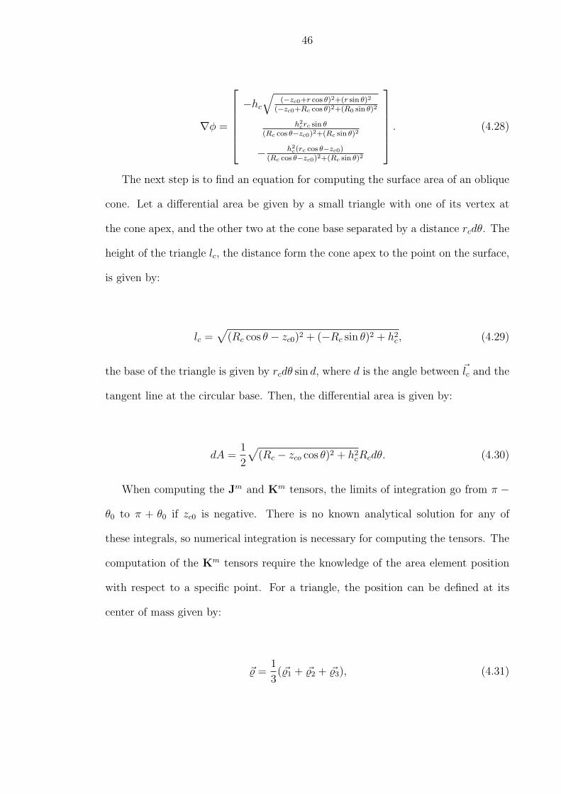
. (4.28)
The next step is to find an equation for computing the surface area of an oblique
cone. Let a differential area be given by a small triangle with one of its vertex at
the cone apex, and the other two at the cone base separated by a distance rcdθ. The
height of the triangle lc, the distance form the cone apex to the point on the surface,
is given by:
lc =√
(Rc cos θ − zc0)2 + (−Rc sin θ)2 + h2c , (4.29)
the base of the triangle is given by rcdθ sin d, where d is the angle between ~lc and the
tangent line at the circular base. Then, the differential area is given by:
dA =1
2
√(Rc − zco cos θ)2 + h2
cRcdθ. (4.30)
When computing the Jm and Km tensors, the limits of integration go from π −
θ0 to π + θ0 if zc0 is negative. There is no known analytical solution for any of
these integrals, so numerical integration is necessary for computing the tensors. The
computation of the Km tensors require the knowledge of the area element position
with respect to a specific point. For a triangle, the position can be defined at its
center of mass given by:
~% =1
3(~%1 + ~%2 + ~%3), (4.31)

47
where the vectors (~%1 ~%2 ~%3) define the position of the triangle vertices relative to a
chosen reference point. If, for instance, the reference point is chosen to be the oblique
cone apex, which represents the sail center, then the element triangle will have its
vertices given by:
~%1 = v3 − v1, (4.32)
~%2 = v3 − v2, (4.33)
~%3 = 0, (4.34)
where
v1 =
0
−Rc sin θ
Rc cos θ − zc0
, (4.35)
v2 =
0
−Rc sin(θ + dθ)
Rc cos(θ + dθ)− zc0
, (4.36)
v3 =
zc0
0
hc
. (4.37)
Let us apply these results to a 100 m by 100 m sail. One triangular quadrant
approximated by an oblique cone will have the following values: hc = 50m, l =
70.71m. Furthermore, if hb is assumed to be 10% of l, then hb = 7.071m, Rc =
180.3m, zc0 = −173.2m, and θ0 = 16.1o.

48
The results were obtained by integration of the equations numerically with a step
size of dθ = 0.0001 radians. Let the force tensors for one of the sail quadrants be
denoted by Jm whose numerical value are
J1 =
−4.0115e− 003
5.4001e− 018
2.5000e− 002
, (4.38)
J2 =
−2.6311e− 004 1.9895e− 019 1.5640e− 003
1.9895e− 019 −1.8641e− 004 −2.5011e− 018
1.5640e− 003 −2.5011e− 018 −9.7788e− 003
, (4.39)
J3ij1 =
−1.0143e− 003 1.7586e− 018 5.7520e− 003
1.7586e− 018 −7.8083e− 004 1.2790e− 018
5.7520e− 003 1.2790e− 018 −3.4308e− 002
, (4.40)
J3ij2 =
1.7586e− 018 −7.8083e− 004 1.2790e− 018
−7.8083e− 004 1.4388e− 018 4.0493e− 003
1.2790e− 018 4.0493e− 003 3.5811e− 017
, (4.41)
J3ij3 =
5.7520e− 003 1.2790e− 018 −3.4308e− 002
1.2790e− 018 4.0493e− 003 3.5811e− 017
−3.4308e− 002 3.5811e− 017 2.1520e− 001
. (4.42)
Following the same procedure, the Km and L tensors are:

49
K2 =
−4.6519e− 017 2.5517e− 002 1.2705e− 016
5.2697e− 002 −3.0070e− 017 −3.2975e− 001
−2.2325e− 017 1.1197e− 002 6.3324e− 017
, (4.43)
K3ij1 =
2.0771e− 016 −1.0689e− 001 −4.8484e− 011
9.6366e + 002 1.6471e− 016 8.3327e + 004
−1.2844e− 011 −4.7425e− 002 −3.0280e− 016
, (4.44)
K3ij2 =
−1.0689e− 001 1.0183e− 013 5.5430e− 001
9.6385e + 002 −1.3610e− 001 8.3326e + 004
−4.7425e− 002 −1.1868e− 011 2.4299e− 001
, (4.45)
K3ij3 =
−9.5444e− 016 5.5430e− 001 −4.8481e− 011
9.6501e + 002 −8.0831e− 016 8.3319e + 004
−1.2844e− 011 2.4299e− 001 1.3193e− 015
. (4.46)
The results for the single quadrant must now be rotated to account for the com-
plete sail geometry. The objective is achieved by performing the rotations about the
zb body-fixed axis, which is parallel to the zc cone-fixed axis, and performing the
transformation outlined in Eq. (3.33). The transformation T is given by:
T =
cos ψ sin ψ 0
− sin ψ cos ψ 0
0 0 1
. (4.47)

50
Since the xc and yc cone axes are not aligned to the xb and yb sail body-fixed
axes, the initial rotation is through 450. The subsequent rotation angles are 1350,
2250 and 3150. After performing these transformations to the J, K, and L integrals
and adding the results, the complete sail integrals obtained are:
J1 =
2.8422e− 014
−2.8422e− 014
1.0258e + 004
, (4.48)
J2 =
5.6634e + 001 8.8818e− 016 2.8422e− 014
8.8818e− 016 5.6634e + 001 −2.8422e− 014
2.8422e− 014 −2.8422e− 014 1.0202e + 004
, (4.49)
J3ij1 =
4.4409e− 016 −3.3307e− 016 5.5988e + 001
−2.2204e− 016 5.5511e− 016 8.8818e− 016
5.5988e + 001 8.8818e− 016 2.8422e− 014
, (4.50)
J3ij2 =
−3.3307e− 016 4.4409e− 016 8.8818e− 016
5.5511e− 016 0 5.5988e + 001
8.8818e− 016 5.5988e + 001 −2.8422e− 014
, (4.51)
J3ij3 =
5.5988e + 001 8.8818e− 016 2.8422e− 014
8.8818e− 016 5.5988e + 001 −2.8422e− 014
2.8422e− 014 −2.8422e− 014 1.0146e + 004
, (4.52)
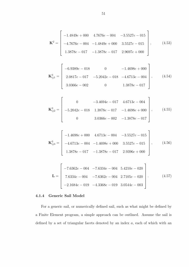
51
K2 =
−1.4849e + 000 4.7676e− 004 −3.5527e− 015
−4.7676e− 004 −1.4849e + 000 3.5527e− 015
1.3878e− 017 −1.3878e− 017 2.9697e + 000
, (4.53)
K3ij1 =
−6.9389e− 018 0 −1.4698e + 000
2.0817e− 017 −5.2042e− 018 −4.6713e− 004
3.0366e− 002 0 1.3878e− 017
, (4.54)
K3ij2 =
0 −3.4694e− 017 4.6713e− 004
−5.2042e− 018 1.3878e− 017 −1.4698e + 000
0 3.0366e− 002 −1.3878e− 017
, (4.55)
K3ij3 =
−1.4698e + 000 4.6713e− 004 −3.5527e− 015
−4.6713e− 004 −1.4698e + 000 3.5527e− 015
1.3878e− 017 −1.3878e− 017 2.9396e + 000
, (4.56)
L =
−7.6362e− 004 −7.6334e− 004 5.4210e− 020
7.6334e− 004 −7.6362e− 004 2.7105e− 020
−2.1684e− 019 −4.3368e− 019 3.0544e− 003
. (4.57)
4.1.4 Generic Sail Model
For a generic sail, or numerically defined sail, such as what might be defined by
a Finite Element program, a simple approach can be outlined. Assume the sail is
defined by a set of triangular facets denoted by an index a, each of which with an

52
area Aa, position (to its center of mass) ~%a, and unit vector normal na. Then the
coefficients for a sail are simply defined as summations over these quantities:
Jm =∑
i
ami nm
i Ai, (4.58)
Km =∑
i
ami %i · nm
i Ai. (4.59)
with these formulae it is simple to compute a sail’s coefficients at any step of the
modeling process.
Let’s apply this approach to a general sail model that is square but non-symmetric.
To generate the sail shape a surface of the form is used:
z = 1−(
1 + cos(πx
l) + ax cos(
fxπx
l) + bx sin(
2πx
l)
) (1 + cos(
πy
l)
+ ay cos(fyπy
l) + by sin(
2πy
l)
), (4.60)
where l is the sail length, a and b are the amplitude of deformations along the x and
y axes, and f is the frequency. a, b, and f allows to change the sail shape easily.
Choosing values of l = 100m, ax = ay = 0.2, bx = by = 0, and fx = fy = 5. The
sail shape for the values is shown in Figure 4.5. Note that this is an arbitrary , but
generally non-symmetric shape, used for example purposes only.
This shape can be modified by assigning values to bx and by. The force and
moment tensor coefficients were computed by discretizing the surface and performing
a numeric integration of all the panels. The resulting GSM tensor coefficients for
this shape are given next:

53
Figure 4.5: Sinusoid Sail Shape.
J1 =
0
0
1.0560E − 001
, (4.61)
J2 =
−1.7835E − 004 5.6948E − 010 −3.9270E − 006
5.6948E − 010 −1.7835E − 004 −3.9270E − 006
−3.9270E − 006 −3.9270E − 006 −4.2180E − 002
, (4.62)
J3ij1 =
−3.2865E − 004 −1.2754E − 007 7.4675E − 003
−1.2754E − 007 −1.2754E − 007 −4.7843E − 008
7.4675E − 003 −4.7843E − 008 3.2878E − 004
, (4.63)

54
J3ij2 =
−1.2754E − 007 −1.2754E − 007 −4.7843E − 008
−1.2754E − 007 −3.2865E − 004 7.4675E − 003
−4.7843E − 008 7.4675E − 003 3.2878E − 004
, (4.64)
J3ij3 =
7.4675E − 003 −4.7843E − 008 3.2878E − 004
−4.7843E − 008 7.4675E − 003 3.2878E − 004
3.2878E − 004 3.2878E − 004 1.7739E + 000
, (4.65)
K2 =
−5.5317E − 007 4.3586E − 004 2.9039E − 005
−4.3586E − 004 5.5317E − 007 −2.9039E − 005
2.0073E − 005 −2.0073E − 005 1.2131E − 018
, (4.66)
K3ij1 =
−5.2438E + 000 1.0109E − 006 −4.6226E − 005
5.2447E + 000 −1.0109E − 006 −1.8246E − 002
−4.6161E − 005 −9.0270E − 019 8.3802E − 004
, (4.67)
K3ij2 =
1.0109E − 006 −5.2446E + 000 1.8246E − 002
−1.0109E − 006 5.2439E + 000 4.6226E − 005
−9.0615E − 019 4.6161E − 005 −8.3802E − 004
, (4.68)
K3ij3 =
−4.6226E − 005 1.8246E − 002 −5.2405E + 000
−1.8246E − 002 4.6226E − 005 5.2406E + 000
8.3802E − 004 −8.3802E − 004 −1.8401E − 017
. (4.69)

55
4.2 Comparison of Sail Geometries
Now that the coefficients for different sail models have been computed, let us
compare the forces generated the flat sail, circular sail, and four-quadrant sail. This
will be done by pitching the sail about the yb body-fixed axis. The sail optical
parameters were chosen as ρ = 0.9, s = 1, Bf = 0.8, Bb = 0.55, εf = 0.05, εb =
0.3. The flat sail area was chosen to be 10000m2. The circular sail is specified by
R0 = 56.42m and αmax = 0.1. All the sails have the same projected area (in the sail
yx-plane)of 10000m2. The resultant normalized forces and normalized moments for
all the geometries ate different sail attitudes are and shown in Figures 4.6 and 4.7,
respectively.
Figure 4.6 shows that the force, normalized by the projected area, generated by
all the sail geometries presented. The force along the zb body-fixed axis is very
similar their since their areas projected to the sun are very similar. The force along
the xb body-fixed axis presents differences for all the sail geometries. The flat sail
produces the lowest magnitude force along this axis. The circular sail has the highest
magnitude due to its concavity. The force from the sinusoid and four-panel sail are
in between these two cases. The force along the yb body-fixed axis is zero for all the
sails for this specific maneuver and no plot is shown.
One effect that is present on flat solar sails is a moment that is dependent on
the sail attitude as predicted in GSM. Figure 4.7 shows the moment, normalized
by the sail area, solar radiation pressure, and characteristic length, for all the sail
geometries except for the flat sail since its moment is zero. When the attitude is
rotated about the x-axis, the moment along the x and z axes are zero for both the
circular and four panel sail. Only the sinusoid sail generates a moment due to its

56
0 20 40 60 80 100−2
−1.8
−1.6
−1.4
−1.2
−1
−0.8
−0.6
−0.4
−0.2
0Fz
α [degrees]
Nor
mal
ized
For
ce
0 20 40 60 80 100−0.16
−0.14
−0.12
−0.1
−0.08
−0.06
−0.04
−0.02
0Fx
α [degrees]
Nor
mal
ized
For
ce
Flat4−PanelSinusoidCircular
Figure 4.6: Normalized force comparison of different sail geometries.
asymmetries even when the sail is directly facing the sun . However, all the sails
produce a moment along the y axis effected by their billow. The highest moment is
produced by the sinusoid sail followed by the four panel sail and the circular sail.
4.3 GSM Partial Derivatives
In this section we derive the partial derivatives of the generalized sail model force
equation. The partial derivatives are required when studying optimization of orbits
and trajectories. We provide first and second order force partial derivatives as may
be required by second-order gradient optimization algorithms. The first force partials
are taken with respect to the position vector, and sail parameters and the second
derivative of the force with respect to the position vector is also derived. The first
and second force partials with respect to the control vector, consisting of the sun-sail
angle and clock angle, are derived as well.
Several of the partial derivatives involve knowing the partial derivative of r with

57
0 50 100−2
0
2
4
6
8
10
12x 10
−4 Mcz
α [degrees]
Nor
mal
ized
Mom
ent
4−PanelSinusoidCircular
0 50 100−2
0
2
4
6
8
10
12
14x 10
−3 Mcy
α [degrees]
Nor
mal
ized
Mom
ent
0 50 100−5
−4
−3
−2
−1
0
1
2
3
4
5x 10
−4 Mcx
α [degrees]
Nor
mal
ized
Mom
ent
Figure 4.7: Normalized moment along the sail body-fixed axes.
respect to itself, which is given by:
∂r
∂r= U− rr = Urr, (4.70)
where U is the identity dyad. We note that any changes in r will be perpendicular
to its direction and cannot be along its direction, hence we see that Urr · r = 0.
Other derivatives that will be needed are:
∂r
∂r=
d(r · r)1/2
dr= (r · r)−1/2r = r, (4.71)
∂r
∂r=
∂
∂r
r
(r · r)1/2=
U
r− r
r
r3=
Urr
r. (4.72)

58
4.3.1 First-Order Partial Derivatives of the Force Equation
Recall the force acting on a solar sail given by [27]:
F = PA[J2 · r− 2r · J3 · r− (J1 · r)r
]. (4.73)
The Jm tensors are defined in Eqs. (3.24)-(3.26) [27]. The force can be thought as
consisting of two functions. One being a function of r only, and the other a function
of the unit position vector r. Thus, the force can be written as:
F = P (r)P(r). (4.74)
The partial derivative of the force with respect to the position vector r can be
expressed using the product rule as:
∂F(r, r)
∂r=
∂P (r)
∂r
∂r
∂rP(r) + P (r)
∂P(r)
∂r· ∂r
∂r, (4.75)
and in tensor notation:
(∂F(r, r)
∂r
)ij
=∂P (r)
∂rrjPi(r) +
P (r)
r
∂Pi(r)
∂rk
∂rk
∂rj
. (4.76)
The partial derivative of the force with respect to r is given by:
∂P(r)
∂r=
[a2J
2 ·Urr − 2ρsr · (J3 ·Urr)− 2ρs(J3 · r) ·Urr
−a3r(J1 ·Urr)− a3(J
1 · r)Urr
]
=[a2J
2 − 4ρsr · J3 − a3rJ1 − a3(J
1 · r)U]·Urr, (4.77)
or in tensor notation:

59
(∂P(r)
∂r
)ik
=[a2J
2ij − 4ρsrmJ3
mij − a3riJ1j − a3J
1mrmUij
]Urrjk, (4.78)
note that:
Urr ·Urr = (U− rr) · (U− rr) = U− rr = Urr, (4.79)
from which it follows that:
(∂P(r)
∂r
)ikUrrkj =
(∂P(r)
∂r
)ij. (4.80)
The partial derivative of the solar radiation pressure with respect to distance
from the sun r is given by:
∂P (r)
∂r= −2πI0R
2s
cr3
√1− R2
s
r2. (4.81)
With all the parameters defined, the force derivative with respect to the position
vector r is given by:
∂F(r, r)
∂r=
∂P (r)
∂rr[a2J
2 · r− 2ρsr · J3 · r + a3(J1 · r)r
]
+P (r)
r
[a2J
2 − 4ρsr · J3 − a3rJ1 − a3(J
1 · r)U]·Urr, (4.82)
which in tensor notation is given by:
Frij =∂P (r)
∂rrj
[a2J
2ilrl − 2ρsrlJ
3likrk + a3J
1l rlri
]
+P (r)
r
[a2J
2il − 4ρsrmJ3
mil − a3riJ1l − a3J
1mrmδil
]Urrlj, (4.83)
where δ is the Kronecker delta function.

60
The force partial derivatives with respect to the optical parameters ρ and s are
given by:
∂F
∂ρ= P (r)
[J2 · r∂a2
∂ρ− 2sr · J3 · r− (J1 · r)r∂a3
∂ρ
]
= P (r)[J2 · r(Bf (1− s)− εfBf − εbBb
εf + εb
)− 2sr · J3 · r + (J1 · r)rs], (4.84)
∂F
∂s= P (r)
[J2 · r∂a2
∂s− 2ρr · J3 · r− (J1 · r)r∂a3
∂s
]
= P (r)[− J2 · rBfρ− 2ρr · J3 · r + (J1 · r)rρ
], (4.85)
∂F
∂Bf
= P (r)[J2 · r ∂a2
∂Bf
]
= P (r)[J2 · r
((1− s)ρ + (1− ρ)
εf
εf + εb
)]. (4.86)
The force partial derivative with respect to Bb, εf , and εb are given by:
∂F
∂Bb
= P (r)J2 · r ∂a2
∂Bb
= −P (r)J2 · r(1− ρ)εb
εf + εb
, (4.87)
∂F
∂εf
= P (r)[J2 · r∂a2
∂εf
]
= P (r)[J2 · r(1− ρ)
Bf
εf + εb
− J2 · r(1− ρ)εfBf − εbBb
(εf + εb)2
], (4.88)
∂F
∂εb
= P (r)[J2 · r∂a2
∂εb
]
= P (r)[− J2 · r(1− ρ)
Bb
εf + εb
− J2 · r(1− ρ)εfBf − εbBb
(εf + εb)2
]. (4.89)

61
Note that the last four equations are linearly dependent and can be expressed
in terms of a known partial derivative. For instance, taking the partial of the force
with respect to Bf as our basis, the other partial derivatives can be expressed as:
∂F
∂Bf
= c1∂F
∂Bb
, (4.90)
∂F
∂Bf
= c2∂F
∂Bb
, (4.91)
∂F
∂εf
= c3∂F
∂Bb
, (4.92)
where
c1 = − 1− ρ
(1− s)ρ +εf
εb(1− sρ)
, (4.93)
c2 = −Bb + Bf
εf + εb
1− ρ
(1− s)ρ +εf
εb(1− sρ)
, (4.94)
c3 =Bb + Bf
εf + εb
1− ρεf
εb(1− s)ρ + (1− sρ)
. (4.95)
4.4 Second-Order Force Partial Derivatives
The second force partial wrt to the position vector r follows from Eq. 4.76:
∂2F(r)
∂r2=
∂2P (r)
∂r2
∂r
∂rrP(r) +
∂P (r)
∂r
∂r
∂rP(r) +
∂P (r)
∂rr∂P(r)
∂r· ∂r
∂r
+∂
∂r
(P (r)
r
)∂r
∂r(∂P(r)
∂r·Urr) +
P (r)
r
( ∂
∂r
)(∂P(r)
∂r·Urr
)· ∂r
∂r, (4.96)
or in tensor form:

62
Frrijk =∂2P (r)
∂r2rkPi(r)rj +
∂P (r)
∂rPi(r)
Urrjk
r+
∂P (r)
∂rrj
(∂P(r)
∂r
)im
Urrmk
r
+∂
∂r
(P (r)
r
)∂Pi(r)
∂rj
rk +P (r)
r
( ∂
∂rm
∂Pi(r)
∂rj
)Urrmk
r. (4.97)
Some of these terms have already been defined. The rest are derived next. The
second partial with respect to r is:
( ∂
∂r
(∂P(r)
∂r·Urr
))ikn
= [−4ρsUrrnmJ3mij − a3J
1jUrrin − a3J
1mUrrmnδij
]Urrjk
+[a2J
2il − 4ρsrmJ3
mil − a3riJ1l − a3J
1mrmUil
](∂Urr
∂r
)lkn
.(4.98)
We also need the second Partial with respect to the distance from the sun r:
∂2P (r)
∂r2=
2πI0R2s
cr6(3r2 − 4Rs2)
(1− R2
s
r2
)−1/2
, (4.99)
and
∂
∂r
(P (r)
r
)=
2πI0
3cr4
[− r2 + r2
(1− R2
s
r2
)1/2
− 4Rs2(1− R2
s
r2
)1/2]. (4.100)
The last term needed is:
∂Urr
∂r= −Urrr− rUrr, (4.101)
which can be expressed in tensor notation:
(∂Urr
∂r
)ijk
= −Urrkirj − riUrrjk. (4.102)
4.5 Force Partial Derivatives with respect to Control Angles
The force partial with respect to the control sun-sail-line angle α and the clock
angle δ can be expressed using the product rule:

63
∂F
∂α= Fr · rα, (4.103)
∂F
∂δ= Fr · rδ, (4.104)
where Fr, rα, and rδ are defined as:
Fr =∂F
∂r, (4.105)
rα =∂r
∂α, (4.106)
rδ =∂r
∂δ. (4.107)
In tensor form Fr is:
Frik =P (r)
r
[a2J
2il − 4ρsrmJ3
mil − a3J1i rl − a3J
1mrmδil
]Urrlk. (4.108)
The unit position vector can be written in terms of the sun-line angle α and the
cone angle δn in the sail-fixed frame as:
r =
− cos δ sin α
− sin δ sin α
− cos α
,
(4.109)
where δn is taken in the positive sense from the x-body-fixed axis.
Now the partial derivatives with respect to the sun-line angle can be evaluated:
rα =
− cos δ cos α
− sin δ cos α
sin α
, (4.110)
and for the cone angle:

64
rδ =
sin δ sin α
− cos δ sin α
0
. (4.111)
The force partial with respect to the control vector u = [α, δ]T is:
Fu =
FTα
FTδ
. (4.112)
4.6 Second Order Force Partial with respect to Control An-gles
The second force partial derivatives with respect to the control angles are again
obtained using the product rule:
∂2F
∂α2=
∂Fr
∂α· rα + Fr · rαα (4.113)
∂2F
∂δ2=
∂Fr
∂δ· rδ + Fr · rδδ (4.114)
∂2F
∂δα=
∂Fr
∂δ· rα + Fr · rαδ, (4.115)
where rαα = ∂2r/∂α2, and similarly for rδδ, and rαδ. Now:
∂Fr
∂α=
∂Fr
∂r· ∂r
∂α= Frr · rα. (4.116)
Computing each of the terms we obtain: Second Partial with respect to r:
Frrikn =P (r)
r[−4ρsUrrnmJ3
mil − a3J1i Urrln − a3J
1mUrrmnδil
]Urrlk (4.117)
+P (r)
r
[a2J
2il − 4ρsrmJ3
mil − a3J1i rl − a3J
1mrmUil
](∂Urr
∂r
)lkn
, (4.118)

65
and similarly for δ. The second partial derivatives of r with respect to the control
angles are:
rαα =
cos δ sin α
sin δ sin α
cos α
, (4.119)
for the cone angle:
rδδ =
cos δ sin α
sin δ sin α
0
, (4.120)
and:
rαδ =
sin δ cos α
− cos δ cos α
0
. (4.121)
The second partial of the force with respect to the control angles are:
Fααi = Frriknrαkrαn + Frikrααk, (4.122)
Fδδi = Frriknrδkrδn + Frikrδδk, (4.123)
Fαδi = Frriknrαkrδn + Frikrαδk. (4.124)
Then the second partial with respect to the control vector u is:
Fuuij1 =
FTαα
FTαδ
, (4.125)

66
Fuuij2 =
FTδα
FTδδ
. (4.126)
4.7 Locally Optimal Control Laws
One advantage to having closed-form equations for the force acting on a solar
sail is that we are able to easily define explicit control and guidance laws. In the
following examples we take the advantage of this to implement simple guidance and
orientation laws for a non-ideal sail. This examples are just meant to showcase how
the GSM can be used analytically, and not meant to provide new results or optimal
sail guidance laws.
4.7.1 Maximum Energy Increase
In Reference [32], a guidance law, using the sun-sail angle as the controller, was
developed to find optimum escape trajectories from the sun using flat, ideal sails. In
this section we extend the locally optimal control law developed in [32] to a four-
quadrant non-ideal billowed solar sail. To accomplish this, the Gauss variational
equation relating the semi-major axis change with respect to the true anomaly can
be written as:
da
df=
2pr2
µ(1− e2)2
e sin f
0
1 + e cos f
· Fp, (4.127)
where µ is the sun’s gravitational parameter, e is the orbit eccentricity, f is the
true anomaly, and Fp is the force expressed in local polar coordinates, p is the semi-
latus rectum, r is the distance form the sun, and a is the orbit semi-major axis. A

67
coordinate transformation T is needed to obtain Fp, as Fp = T · F, where F is the
sail force in the body-fixed frame. The relationship between these two coordinate
frames is shown in Figure 4.8.
Sail Trajectory
er
erxq
eq
ez
ey
ex
a
Figure 4.8: Local polar coordinate frame and sail body-fixed frame.
We only consider changes in the sail position and attitude in the orbit plane (i.e.,
set δf ≡ 0). Then T is given by:
T =
− sin α 0 − cos α
0 −1 0
cos α 0 − sin α
, (4.128)
where Fp has radial Fr, out of plane Fr×θ, and transverse Fθ force components.
Finding the maximum energy increase at any point on the sail trajectory is equivalent
to finding the maximum rate of change of da/df with respect to the sun-sail angle.
Taking the partial derivative of Eq. (4.129) yields:

68
∂
∂α
(∂a
∂f
)=
2pr2
µ(1− e2)2
e sin f
0
1 + e cos f
·(∂T
∂α· F + T · ∂F
∂α
). (4.129)
The partial of T with respect to α is readily obtained from Eq. (4.128) and the
partial of F with respect to α is given by Eq. (4.103). Setting the above equation
equal to zero for the square-billowed sail model (coefficients found in Section 4.1.3),
the optimal angle satisfies the relation:
0 = 1.9201(1 + e cos f)− 5.7604e sin f tan α− 3.7804(1 + e cos f) tan2 α
−0.0599e sin f tan3 α. (4.130)
The solution of Eq. (4.130) is chosen so that Eq. (4.127) is maximized. The
control law equation is close to the solution for an ideal flat solar sail. The force
acting on an ideal flat sail in the local polar frame is given by:
Fp = 2P (r)A
cos3 α
0
sin α cos2 α
. (4.131)
With this information the equation for the optimum angle is obtained from:
0 = 2(1 + e cos f)− 6e sin f tan α− 4(1 + e cos f) tan2 α. (4.132)
The solution of the above equation is obtained by solving the quadratic equation
for tan α and is presented in [32]. Both the ideal and the optimum control laws can
be compared now on the squared-billowed sail model. Figure 6.2 is polar plot of the

69
orbit change using both guidance laws starting at 1 AU during a time of one year.
The optimum control law has a faster energy increase, as expected. The orbital
energy increase for both guidance laws is shown in Figure 4.10, which clearly shows
that the non-ideal guidance law is optimum. The values for the optical parameters
used in the simulation were ρ = 0.9, s = 1, Bf = 0.8, Bb = 0.5, εf = 0.05, εb = 0.3
and the mass chosen was 80kg.
1.000000e+011
2.000000e+011
3.000000e+011
4.000000e+011
30
210
60
240
90
270
120
300
150
330
180 0
Realistic LawIdeal Law
Figure 4.9: Trajectories for realistic and ideal guidance laws.
Thus, it was shown that the generalized sail model can be applied to more complex
sail geometries resulting in more realistic guidance laws development.
4.7.2 Maximum Propulsive Force
As another example, we can compute the planar orientation that gives the max-
imum propulsive force on the sail. This can be found by differentiating the square

70
0 50 100 150 200 250 300 350 400−10
−9
−8
−7
−6
−5
−4x 10
8
time (days)
Ene
rgy
(m2 /s
2 )
Realistic LawIdeal Law
Figure 4.10: Energy increase for realistic and ideal guidance laws.
of the force magnitude with respect to the sun-sail angle and setting the resulting
expression equal to zero:
∂(F · F)
∂α= 2F · ∂F
∂α= 0. (4.133)
The corresponding equation for the four-quadrant sail example is:
(− 3.3735− 3.3040 cos 2α
)cos α sin α = 0, (4.134)
which has its extrema when α equals 0, π/2, π, and 3π/2. The term in the parenthesis
is zero for α complex. These solutions are the same as that of an ideal solar sail.
When α = 0, the maximum force is achieved, and with α equal to π/2 or 3π/2, the

71
force is zero. Finally, the solution α = π implies that the sail is facing away from the
sun, an orientation we do not consider. This simple result occurs due to the overall
symmetry of the four quadrant sail.
Now we consider a more general situation. Let us find the sun-sail angle that
provides the maximum force for only one quadrant of the square-billowed sail whose
force tensors coefficients are given in Section 4.1.3. Following the same procedure as
for the complete sail, the equation that needs to be satisfied is now:
−83.806− 759.262 tan α + 248.428 tan2 α− 27.134 tan3 α + tan4 α = 0. (4.135)
This equation has only two real solutions, −6.0960 and 83.9130. The first solution
maximizes the force on the sail; the sign is negative due to the quadrant position
with respect to the overall sail (the opposite quadrant would have the reverse sign
on the solutions). The second solution minimizes the force on the sail. These exam-
ples showcase the ease with which we can work with complex sail shapes using the
generalized sail model.
4.8 Applications of GSM to NASA’s S5 Project
The study of mission design for solar sails possesses some unique problems that
cannot be fully studied with tools existing for other type of spacecraft. Some of these
issues are the sail controllability and the fact that the thrust vector is dependent
on the sail attitude [12]. The Solar Sail Spaceflight Simulation Software (S5) is
an integrated set of high fidelity software modules that enables the analysis of the
optimal design of solar sail trajectories and of the guidance, navigation and control
of these missions. Prior to S5 there was no single integrated tool that allowed this
analysis [7].

72
S5 is a modular tool composed of several subroutines that can used in conjunction
to study all the aspects of a solar sail mission or individually to study a specific part
of the mission.
The Mission Design Module (OPT) determines the optimal trajectory and sail op-
timal control with respect to a given performance criteria subject to control and/or
state constraints. A second order-gradient optimization algorithm is used to con-
verge to the optimal trajectory, which uses the force partial derivatives of the GSM
developed in Section 4.3.
The Solar Radiation Pressure Module (SRP) models the force and moment acting
on the sail due to the solar radiation pressure, which are used by the OPT, ADC,
and DET modules. The inputs for the SRP are the sail physical characteristics
and optical properties, sailcraft state and attitude, and attitude control vanes (if
available) position relative to the sail to compute the thrust and the total torque due
to solar radiation pressure.
The Attitude Dynamics and Control Module (ADC) simulates the rotational
dynamics of the solar sail, including torque induced by solar radiation pressure,
environmental disturbances such as gravity gradient, aerodynamic, and magnetic
moment, and conventional spacecraft actuators such as reaction wheel assembly and
thrusters. Some of the attitude control methods used are articulated control vanes
located at the sail tips and mass displacement. The ADC module takes into account
structural dynamical effects.
The Trajectory Control Module (TCN) updates the thrust control profile based
on the current estimate of the spacecraft state, provided by the Orbit Determination
Module, and the nominal sail state trough a feedback control law. TCN uses the gain
matrix from OPT and feedback control laws to update the control and predict the

73
updated target conditions. The commanded controls are fed into the ADC module.
The Orbit Determination Module (DET) simulates the navigation of the solar
sail. DET propagates the equations of motion, simulates ground based and on board
observations and processes the observables with a Kalman type filter to estimate
the current state and statistics. DTE allows for covariance analysis or Monte Carlo
studies.
The integrated version of S5 illustrating all the interaction and data flow between
modules is shown in Figure 4.11.
Some of the outputs to evaluate the performance consists of optimal trajectories,
control profiles and measures of performance, sailcraft attitude, angular velocity and
angular acceleration, sailcraft control surface deflection angles for vanes systems,
estimates and uncertainties of spacecraft position and and other dynamic parameters
[7].
The organizations involved in the development of S5 were the Jet Propulsion
Laboratory in charge of the OPT and DTE modules as well as integrating of all
the modules into a complete software package. The University of Michigan which
contributed in the development of SRP module, force and moment parameter es-
timation, and force partial derivatives. Ball Aerospace was in charge of the ADC
module. The University of Colorado developed the TCN module. LGarde Inc. pro-
vided nominal sail design shape and measured force and moment characterization.
NASA Marshall supervised the development of S5 to fulfill requirements, to stay on
schedule, and to evaluate the progress on each of the three phases of development.

74
Figure 4.11: Integration of S5.

CHAPTER V
Estimation: Force, Moment, and Optical
Parameters
As with all space missions, success depends on having a precise spacecraft model.
Initial mission planning can be performed based on data from ground measurements.
However, due to the complexity of sail shapes a refinement of the sail propulsion
model will be necessary after launch for navigating the sail to its target. Sail wrinkles
after in-space deployment, deformation from ideal shapes, and surface degradation
due to the space environment[20] are some of the effects that make pre-launch sail
propulsion determination inaccurate.
The generalized sail model [27] allows for the analytic computation of forces and
moments acting on a solar sail of arbitrary fixed shape. The generalized equations for
the sail force and moment are linear in the GSM coefficients. This fact and its analytic
nature allows us to develop linear estimation methods for these coefficients using
measured accelerations and moments as input data. The force and moment tensor
coefficients are estimated using a least-squares algorithm from simulated navigation
data and predictions from finite element models of solar sails. The estimation results
are highly dependent on the attitudes at which the sail navigation data is taken. It is
not only important to take measurements at several different sun-relative attitudes,
75

76
but also to find those attitudes that capture the geometry of the sail. The accuracy
of the estimates will vary for different data sampling strategies. Here, we present
several data sampling examples and comment on their impact to the accuracy of the
estimation results.
5.1 Linear Estimation of GSM Tensor Coefficients
In the following the sail force and moments are reported in a normalized form
by dividing the force values by the solar radiation pressure and total sail area and
the moments by an additional reference length lr [5]. Thus, the force and moment
vectors can be written as:
F = PACF , (5.1)
M = PAlrCM , (5.2)
where C is a vector containing the normalized values with the subscripts denoting
force or moment.
In the following we assume that the navigation data is reported as normalized
force and moment vectors. The normalized version of the GSM equations are:
Fc = J2 · r− 2r · J3 · r− (J1 · r)r, (5.3)
Mc = K2 · r + r ·K3 · r. (5.4)
Force and moment can be obtained from measurements taken through on-board
instruments such as inertial measurement units, gyroscopes, and with ground track-
ing. Note that the measured on-board rotational accelerations must be related, via

77
the moment of inertia, to the total moment acting on the sailcraft. We do not
consider the estimation of the inertia tensor or sailcraft mass in our current work.
5.2 Force and Moment in Linear Form
The normalized force and moment are linear in all the coefficients of the Jm and
Km tensors, thus a least-squares estimation can be easily employed for finding the
best values of the tensor coefficients. But before this step is done, it is necessary
to manipulate the equations and write them in a more useful way as the product of
a matrix and a vector. The matrix contains information on the sail attitude while
the vector contains the tensor coefficients that need to be estimated. Thus, the
normalized force can be written as:
Fc = AF (r)J, (5.5)
where the matrix AF is 3 × 19 and a function of the sail attitude alone, and J is a
19× 1 vector containing the independent force tensor coefficients.
The force matrix is defined as follows:
AF =
[−AF1 AF2 −2AF3
], (5.6)
where
AF1 =
r21 r1r2 r1r3
r1r2 r22 r2r3
r1r3 r2r3 r23
, (5.7)

78
AF2 =
r1 r2 r3 0 0 0
0 r1 0 r2 r3 0
0 0 r1 0 r2 r3
, (5.8)
AF3 =
r21 2r1r2 r2
2 2r2r3 2r1r3 r23 0 0 0 0
0 r21 2r1r2 2r1r3 0 0 r2
2 2r2r3 r23 0
0 0 0 2r1r2 r21 2r1r3 0 r2
2 2r2r3 r23
. (5.9)
For one measurement the rank of Af is 3. Thus, more than one measurement is
needed to estimate a uniquely a full set of force coefficients. This is accomplished by
taking at least 7 measurements at different sun-sail attitudes. The force coefficient
vector is
J =
[J1
1 J12 J1
3 J211 J2
12 J213 J2
22 J223 J2
33 J3111
· · ·
· · · J3121 J3
221 J3231 J3
131 J3331 J3
222 J3232 J3
332 J3333
]T
. (5.10)
Similarly, the moment equation also can be written as the product of a matrix,
which contains information on the sail attitude at which the measurements are taken,
and a vector, which includes the information of the moment tensor coefficients:
Mc = AMK, (5.11)
where

79
AM =
[AM2 AM3
], (5.12)
AM2 =
r1 r2 r3 0 0 0 0 0 0
0 0 0 r1 r2 r3 0 0 0
0 0 0 0 0 0 r1 r2 r3
, (5.13)
AM3 =
r21 r1r2 r1r3 r1r2 r2
2 r2r3 r1r3 r2r3 r23
0 r21 0 0 r1r2 0 0 r1r3 0
0 0 r21 0 0 r1r2 0 0 r1r3
· · ·
· · ·0 0 0 0 0 0 0 0 0
r1r2 r1r3 r22 r2r3 r2r3 r2
3 0 0 0
0 r1r2 0 r22 0 r2r3 r1r3 r2r3 r2
3
. (5.14)
AM is rank-3 in general. Since the moment requires 27 coefficients at least 9
measurements are necessary. There are, however, certain attitudes that must be
avoided to have a full rank matrix. With 9 measurements a matrix of rank-27 can be
achieved under the conditions that no measurements are taken when either r1 or r2
are equal to zero or equal to r3, or when r1 = r2. Thus, if the above requirements hold
for the moment measurements, then the coefficients of K2 and K3 can be determined
uniquely. The vector with the moment coefficients is:
K =
[K2
11 K212 K2
13 K221 K2
22 K223 K2
31 K232 K2
33 K3111 K3
121 K3131
· · ·

80
· · · K3211 K3
221 K3231 K3
311 K3321 K3
331 K3122 K3
132 K3222 K3
232· · ·
· · · K3322 K3
332 K3133 K3
233 K3333
]T
. (5.15)
5.3 Least-Squares Estimation
For estimating the GSM tensor coefficients, a least-squares cost function is em-
ployed with the assumption of N measurements taken at different sun-relative atti-
tudes. A covariance matrix Pcc, associated with the measurements y, is given by:
Pcc = E[(yj − yj)(yj − yj)
T], (5.16)
where E[ ] is the expected value operator. Ideally
Pcc =
σ2ω 0 0
0 σ2ω 0
0 0 σ2ω
, (5.17)
which is the covariance matrix for uncorrelated measurements with variance σ2ω. Note
that the yj vectors are either normalized force or moment measurements, depending
on the application.
The least-squares cost function is defined as the square of the error between the
measurements and the values due to estimated coefficients. Hence it is given by
V =1
2
N∑j=1
(yj −Ajx)T P−1cc (yj −Ajx) , (5.18)
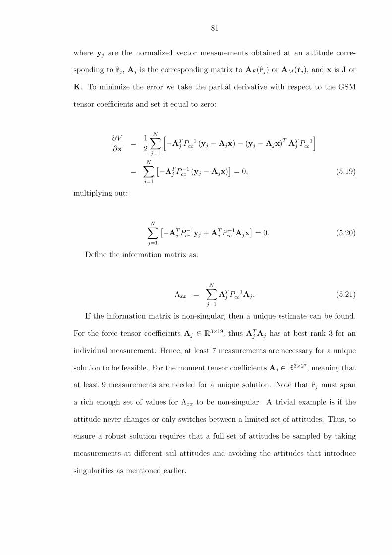
81
where yj are the normalized vector measurements obtained at an attitude corre-
sponding to rj, Aj is the corresponding matrix to AF (rj) or AM(rj), and x is J or
K. To minimize the error we take the partial derivative with respect to the GSM
tensor coefficients and set it equal to zero:
∂V
∂x=
1
2
N∑j=1
[−AT
j P−1cc (yj −Ajx)− (yj −Ajx)T AT
j P−1cc
]
=N∑
j=1
[−ATj P−1
cc (yj −Ajx)]
= 0, (5.19)
multiplying out:
N∑j=1
[−ATj P−1
cc yj + ATj P−1
cc Ajx]
= 0. (5.20)
Define the information matrix as:
Λxx =N∑
j=1
ATj P−1
cc Aj. (5.21)
If the information matrix is non-singular, then a unique estimate can be found.
For the force tensor coefficients Aj ∈ R3×19, thus ATj Aj has at best rank 3 for an
individual measurement. Hence, at least 7 measurements are necessary for a unique
solution to be feasible. For the moment tensor coefficients Aj ∈ R3×27, meaning that
at least 9 measurements are needed for a unique solution. Note that rj must span
a rich enough set of values for Λxx to be non-singular. A trivial example is if the
attitude never changes or only switches between a limited set of attitudes. Thus, to
ensure a robust solution requires that a full set of attitudes be sampled by taking
measurements at different sail attitudes and avoiding the attitudes that introduce
singularities as mentioned earlier.

82
The covariance matrix of the estimates is Pxx = Λ−1xx . Then, the solution of the
estimation problem can be written as [13]:
x = Pxx
N∑j=1
ATj P−1
cc yj. (5.22)
Defining the data vector Z as:
Z =N∑
j=1
ATj P−1
cc yj, (5.23)
the solution of x can be expressed in a compact more form as:
x = PxxZ. (5.24)
5.3.1 Predicted Force and Moment Uncertainty
Note that the predicted normalized force and moment at an attitude r can then
be written in the form
y = A(r)PxxZ, (5.25)
where the matrix A(r) is a function of the attitude and y is the predicted force or
moment.
Uncertainties in the tensor coefficients translate into force or moment uncer-
tainties. The mapping from tensor coefficients uncertainties into normalized vector
uncertainties is given by:
δy = A(r)δx. (5.26)

83
The covariance of the estimates is obtained by
Pyy = E[δyδyT ] = A(r)E[δxδxT ]AT (r), (5.27)
which is just
Pyy = A(r)PxxAT (r), (5.28)
where Pxx is the covariance of the estimated GSM tensor coefficients, and equals Λ−1xx .
Pxx allows us to place bounds on the errors of the force and moment estimation. Thus,
the force and moment covariance at a given attitude are
PFF = AF (r)PJJATF (r), (5.29)
PMM = AM(r)PKKATM(r), (5.30)
respectively.
5.4 Numerical Linear Estimation
Due to the lack of actual navigation data, the square sinusoid sail, developed
in Chapter IV, was used to generate simulated forces and moments at different sail
attitudes. These force and moments were used to recover the force and moment
tensors using the estimation algorithm developed and the results are shown next.
5.4.1 Force Estimation
The results from the estimation are dependent on how the sampling of the mea-
surements is performed as is shown in the following test cases and can be seen from
Eqs. (5.24) and (5.21) as A is dependent on the sail attitude when data is collected.
In these figures, the covariance of each force tensor coefficient is shown as well as
the correlation between them. Four cases with 70 measurements each, but with

84
different measurement sampling attitudes, were used for estimating the tensor coef-
ficients. Comparison between their respective covariance and correlations are shown
in Figures 5.5-5.12.
The case studies are defined as follows: Case I has measurements running along
the two diagonals 450 from the x and y body-fixed axes as shown in Figure 5.1.
−0.8 −0.6 −0.4 −0.2 0 0.2 0.4 0.6 0.8−0.8
−0.6
−0.4
−0.2
0
0.2
0.4
0.6
0.8
ri
r j
Figure 5.1: Case I. Projected attitude measurements
Case II has measurements taken along the x and y body-fixed axes as shown in
Figure 5.2.
Case III forms a 4-loop curve in the xy-plane, while Case IV forms a spiral as
shown in Figures 5.3 and 5.4.

85
−1 −0.5 0 0.5 1−1
−0.8
−0.6
−0.4
−0.2
0
0.2
0.4
0.6
0.8
1
ri
r j
Figure 5.2: Case II. Projected attitude measurements
−0.8 −0.6 −0.4 −0.2 0 0.2 0.4 0.6 0.8−0.8
−0.6
−0.4
−0.2
0
0.2
0.4
0.6
0.8
ri
r j
Figure 5.3: Case III. Projected attitude measurements

86
−1 −0.5 0 0.5 1−1
−0.8
−0.6
−0.4
−0.2
0
0.2
0.4
0.6
0.8
1
ri
r j
Figure 5.4: Case IV. Projected attitude measurements
1 2 3 4 5 6 7 8 9 10 11 12 13 14 15 16 17 18 190
0.1
0.2
0.3
0.4
0.5
0.6
0.7
0.8J Coefficient Covariance
J Coefficient Element
Cov
aria
nce
Figure 5.5: Case I. Covariance of GSM force coefficients

87
1 2 3 4 5 6 7 8 9 10 11 12 13 14 15 16 17 18 190
0.1
0.2
0.3
0.4
0.5
0.6
0.7
0.8J Coefficient Covariance
J Coefficient Element
Cov
aria
nce
Figure 5.6: Case II. Covariance of GSM force coefficients
1 2 3 4 5 6 7 8 9 10 11 12 13 14 15 16 17 18 190
0.02
0.04
0.06
0.08
0.1J Coefficient Covariance
J Coefficient Element
Cov
aria
nce
Figure 5.7: Case III. Covariance of GSM force coefficients

88
1 2 3 4 5 6 7 8 9 10 11 12 13 14 15 16 17 18 190
0.1
0.2
0.3
0.4
0.5
0.6
0.7
0.8J Coefficient Covariance
J Coefficient Element
Cov
aria
nce
Figure 5.8: Case IV. Covariance of GSM force coefficients
1 2 3 4 5 6 7 8 9 10111213141516171819
12345678910111213141516171819−1
−0.5
0
0.5
1
J Coefficient Element
Correlation
J Coefficient Element
Cor
rela
tion
Figure 5.9: Case I. Correlation of GSM force coefficients

89
1 2 3 4 5 6 7 8 9 10111213141516171819
12345678910111213141516171819−1
−0.5
0
0.5
1
J Coefficient Element
Correlation
J Coefficient Element
Cor
rela
tion
Figure 5.10: Case II. Correlation of GSM force coefficients
1 2 3 4 5 6 7 8 9 10 11 12 13 14 15 16 17 18 19
12345678910111213141516171819−1
−0.5
0
0.5
1
J Coefficient Element
Correlation
J Coefficient Element
Cor
rela
tion
Figure 5.11: Case III. Correlation of GSM force coefficients

90
1 2 3 4 5 6 7 8 9 10 11 12 13 14 15 16 17 18 19
12345678910111213141516171819−1
−0.5
0
0.5
1
J Coefficient Element
Correlation
J Coefficient Element
Cor
rela
tion
Figure 5.12: Case IV. Correlation of GSM force coefficients
In practice, the sail would be re-oriented to these different attitudes during a
characterization phase and the accelerations and moments measured using on-board
inertial measuring units (IMUs). The projected sail attitude is a plot of the y com-
ponent versus the x component of r on the sail xy-plane. Figures 5.5-5.8 show the
covariance for each of four cases described. Case III is the data sampling with the
lowest covariance. Figures 5.9-5.12 shoe the correlation of for the force tensor coeffi-
cients. The correlations of a given tensor coefficient with itself are suppressed from
the plots since by definition it is unity. From these figures it can be seen that case
III has the lowest covariance and correlation.
Figure 5.13 show the force covariance for each of the four cases as obtained from
Eq. (5.28). Cases I and II have similar force covariance along all axes. Cases I, II,
and IV perform similarly along the x-axis. Along the z-axis case III performs better
at high sun-sail angles α.

91
All the cases have very similar results for the estimated force and comparable
errors, showing that the estimation process converges upon the correct values. Figure
5.14 shows representative results of the actual normalized force of the sinusoid sail
and the estimated normalized force as well as their respective error.
0 10 20 30 40 50 60 70 80 900
0.1
0.2
Pffx
0 10 20 30 40 50 60 70 80 900
0.2
0.4
Pffy
0 10 20 30 40 50 60 70 80 900
0.5
1
α (deg)
Pffz
Case I
Case II
Case III
Case IV
Figure 5.13: Force Covariance.
5.4.2 Moment Estimation
The moment covariance and correlation were computed for measurements as in
Cases III and IV and are shown in Figures 5.15-5.18. Case I has measurements when
r1 or r2 are zero and Case II has measurements when r1 = r2. Both situations make
AM rank deficient and ΛMM singular and were not used in the estimation.
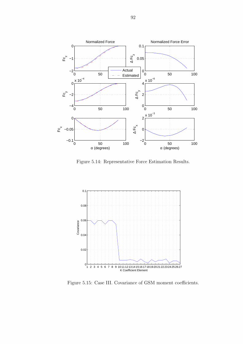
92
0 50 100−2
−1
0
Fc z
Normalized Force
ActualEstimated
0 50 100−4
−2
0x 10
−4
Fc y
0 50 100−0.1
−0.05
0
Fc x
α (degrees)
0 50 1000
0.05
0.1
∆ F
c z
Normalized Force Error
0 50 1000
2
4x 10
−6
∆ F
c y
0 50 100−2
0
2x 10
−3
∆ F
c x
α (degrees)
Figure 5.14: Representative Force Estimation Results.
1 2 3 4 5 6 7 8 9 1011 1213141516 1718192021 2223242526 270
0.02
0.04
0.06
0.08
0.1
K Coefficient Element
Cov
aria
nce
Figure 5.15: Case III. Covariance of GSM moment coefficients.

93
1 2 3 4 5 6 7 8 9 1011 1213141516 1718192021 2223242526 270
0.1
0.2
0.3
0.4
0.5
0.6
0.7
0.8
K Coefficient Element
Cov
aria
nce
Figure 5.16: Case IV. Covariance of GSM moment coefficients.
1 2 3 4 5 6 7 8 9 10 11 12 13 14 15 16 17 18 19 20 21 22 23 24 25 26 27
123456789101112131415161718192021222324252627−1
−0.8
−0.6
−0.4
−0.2
0
0.2
0.4
0.6
0.8
1
K Coefficient ElementK Coefficient Element
Figure 5.17: Case III. Correlation of GSM moment coefficients.

94
1 2 3 4 5 6 7 8 9 10 11 12 13 14 15 16 17 18 19 20 21 22 23 24 25 26 27
123456789101112131415161718192021222324252627−1
−0.8
−0.6
−0.4
−0.2
0
0.2
0.4
0.6
0.8
1
K Coefficient Element
Correlation. Case IV.
K Coefficient Element
Figure 5.18: Case IV. Correlation of GSM moment coefficients.
0 50 100−1
0
1
2x 10
−3 Mcz
Mcz
ActualEstimated
0 50 100−0.01
0
0.01
Mcy
Mcy
0 50 100−1
0
1x 10
−3 Mcx
α (degrees)
Mcx
0 50 100−4
−2
0
2x 10
−5 ∆ Mcz
∆ M
cz
0 50 1000
0.5
1x 10
−3 ∆ Mcy
∆ M
cy
0 50 100−6
−4
−2x 10
−5 ∆ Mcx
α (degrees)
∆ M
cx
Figure 5.19: Representative Moment Estimation Results.

95
The moment coefficients were estimated and the moment results for each of the
two cases were compared with the actual moment generated by the sinusoid sail.
Both Cases III and IV replicate the sail moment although with comparable errors as
shown representatively in Figure 5.19. This estimation was performed with 70 data
measurements. Note the poor performance of Case IV covariance when compared to
Case III.
One last case was carried out by performing a uniform data sampling across all
the sail possible attitudes. The sampling was done with 8100 data measurements.
The moment covariance shrinks to zero. The estimation was successful in recovering
the moment generated by the sail with small deviations from the actual values and
slight improvements over the previous two cases.
5.5 Symmetric Sail Shapes
In Chapter III it was shown earlier that for symmetric sails the number of coeffi-
cients needed to model their generated force and moment are greatly reduced. Thus,
the amount of measurements needed for their estimation is reduced. In the rest of
this chapter, the force and moment equations for the GSM parameter estimation are
developed for a two-axis symmetric sail.
5.5.1 Force Tensor Coefficients
With these simplifications, the normalized force for a two-axis symmetric sail
becomes

96
F = PA
r1 0 0 −4r1r3 0 0 −r1r3
0 r2 0 0 −4r2r3 0 −r2r3
0 0 r3 −2r21 −2r2
2 −2r23 −r2
3
J211
J222
J233
J3131
J3232
J3333
J13
. (5.31)
5.5.2 Moment Tensor Coefficients
For a 2-axis symmetric sail the terms K212, K2
21, K3213, K3
321, and K3132 are non-zero
in general. Thus, for a 2-axis symmetrical sail the matrices given by Eqs. (5.13)-
(5.14) reduce to
A2M =
r1 0
0 r2
0 0
, (5.32)
ALM =
r2r3 r2r3 0
0 r1r3 r1r3
r1r2 0 r1r2
, (5.33)
and the vector with the independent moment tensor coefficients is
K =
[K2
12 K221 K3
213 K3321 K3
132
]. (5.34)

97
5.6 Discussion
In this chapter a methodology for estimating the forces and moments acting
on a sail of arbitrary shape is presented based on the generalized sail model. The
estimation is based on a least-squares algorithm. The accuracy of the estimation was
dependent on the sail attitude relative to the sun when the measurement sampling
was taken. The moment estimation is more sensitive to the data sampling; cases
when r1 or r2 are zero or equal to r3 and r1 = r2 should be avoided for the moment
estimation.
A non-symmetric sinusoid sail shape was used to simulate force and moment data.
Forces and moments were estimated based on these data. Four different cases of
data samplings were used to estimate the forces. All four cases recovered the force
from the sinusoid sail with small errors. The moment tensor coefficients were also
estimated using a least squares algorithm.
The estimation of both the force and moment included the optical parameters in the
definition of the tensor coefficients, which made possible to estimate their combina-
tion. Since the tensor coefficients and optical parameters appear as a product there
is no need to estimate them separately.
Finally, it was shown that symmetric sails required fewer tensor coefficients to capture
the force and moment acting upon them. A 2-axis discretely symmetrical sail requires
7 coefficients for the force and 5 coefficients for the moment. A Sail with rotational
symmetry requires only 5 coefficients for the force and 2 for the moment.

CHAPTER VI
Solar Sail Trajectory Control
Solar sail missions must be designed for a specific sail propulsion model [2, 19].
However, due to the complexity of solar sails and difficulties in providing precise
predictions of their performance, our ability to precisely predict the sail acceleration
performance is inherently limited. To account for this, trajectory design of a sail
mission must be performed with a conservative propulsion model that provides ad-
equate margin for uncertainties in the sail performance. Specifically, it is important
that the sail provide a guaranteed minimum amount of thrust to ensure that the
chosen mission can be flown. Due to this, however, the actual sail will most likely
always have more thrust than the original mission planned for. Due to the nature
of solar sails, this excess thrust cannot be easily modulated and will fundamentally
change the trajectory of the sail and may make it difficult to achieve mission targets.
While it is possible to estimate the actual sail propulsion after deployment and re-
design the sail trajectory [30], this constitutes an open and continual design process
that may not always be feasible to implement and which may not converge on the
proper target. Similarly, as the sail surface suffers from degradation [20] throughout
the mission, the thrust will change continuously and, if the maximum thrust of the
sail is being used, constant re-optimization and redesign of the trajectory would be
98

99
necessary.
Previously, trajectory control laws have been developed for the same sail per-
formance as the trajectory was designed for. In Reference [16], a trajectory control
methodology is developed for stationing a solar sail at a sub-L1 point and is noted
the difficulties of achieving the mission objectives. In Reference [15] is suggested
to use a sail with varying area in order to increase the control authority of the sail
on a transfer trajectory. However, a sail with varying area may not be feasible to
implement.
In this chapter we consider the case for controlling a sail with excess performance
about a nominal trajectory. A sail with excess performance does not require a con-
tinually redesigned trajectory, as the sail properties change over time, it also does
not require a varying area and still provides enough control authority to follow the
mission. Our approach will allow a sail to follow a nominal mission design so long
as the sail provides an excess of thrust, which will be the nominal design situation
for any sail mission. Ideally, our approach can be applied to any trajectory, and
will allow the sail to follow a nominal mission profile. In this chapter we consider
the problems of maintaining a sail at a specific sub-L1 equilibrium point location as
well as tracking a moving point in a halo orbit about a sub-L1 point. This work
can be generalized to tracking an arbitrary trajectory as they can be considered as a
sequence of moving points. The flat, ideal sail model is used throughout this chapter.
The results can be generalized to real sail models using the GSM.
Consider the example of maintaining a specific sub-L1 equilibrium point location.
In general, if the sail generates less thrust than the design performance, it will not
be possible for it to maintain this position and the mission cannot be achieved. If it
has precisely the design performance, then it is possible to maintain the equilibrium

100
point and even perform control maneuvers to maintain itself close to this location,
accounting for errors in initial condition and other factors [19]. If the sail has more
thrust than its design performance, however, it becomes difficult to maintain the
target location without actively modulating the total surface area of the sail. Such
modulation would be a difficult and complex procedure to carry out with the sail
structure.
The main problem in this situation is that the sail has excess thrust. A simple
solution is to orient the sail so that it provides the appropriate thrust level along
the line connecting the two primaries (the line of syzygies), and “dump” the excess
thrust along the direction perpendicular to this line. In a short time, of course, the
sail would veer off course and leave the equilibrium. A simple fix would be to switch,
or dither, the sail back and forth – maintaining the proper thrust along the line of
syzygy and producing a net zero thrust perpendicular to this line. Such an approach
may work conceptually, but may be difficult to implement. Problems with this idea
arise in changing the sail sense of rotation to average the perpendicular force to
zero. Also, the dithering approach would be insufficient for tracking a non-planar
trajectory in three-dimensions. Following this line of thought, however, we find a
simple approach that can essentially achieve this goal of maintaining the appropriate
thrust vector and forcing the excess thrust to average out to zero.
To accomplish this task we force the sail to “orbit” the equilibrium point (or a
nominally moving point along a trajectory) in a small orbit centered on this nominal
solution. Instead of forcing the sail to dither back and forth, however, we have the
sail follow a near circular path about the nominal solution that has a centripetal
acceleration equal to the amount of excess thrust generated after the sail is oriented
to provide the nominal thrust. Thus, the sail will follow the nominal trajectory while

101
performing a controlled “orbit” about the trajectory. For a given value of excess
thrust there is some freedom in designing this orbit, as the centripetal acceleration
depends on both the radius of this orbit and the angular rate.
This control approach can be implemented by inducing the sail to rotate at the
same rate as it “orbits” the nominal solution. Thus the attitude of the sail is fixed
such that the excess thrust is always pointed towards the nominal solution. However,
there may be instances where the excess force is modulated away from the center of
rotation for control.
6.1 Circular Restricted Three Body Problem in CylindricalCoordinates
If the sail produces a higher force than originally expected, then it cannot be
stationed at the sub-L1 point. One solution is to recompute a new sub-L1 point
x′L1< xL1 , however, this approach may force the sail to fly in a regime that it was
not designed for. Another possibility is to used the extra force to orbit the sub-
L1 point. The second option provides a better approach since it allows the sail to
maintain the required xL1 location.
For orbiting the sub-L1 point it is helpful to write the circular, restricted, three-
body problem equations of motion in a cylindrical coordinate frame rotating about
the nominal equilibrium as shown in Figure 6.1. This describes a cylindrical coordi-
nate frame with its axis of symmetry along the x-axis. Let y = r cos θ and z = r sin θ.

102
y
x
za
ax
aq
ar
q
r
Figure 6.1: Sail in Orbit about Sub-L1 Point.
The kinematics of the y and z coordinates in the new variables is:
y = r cos θ − rθ sin θ, (6.1)
z = r sin θ + rθ cos θ, (6.2)
y = r cos θ − 2rθ sin θ − rθ2 cos θ − rθ sin θ, (6.3)
z = r sin θ + 2rθ cos θ − rθ2 sin θ + rθ cos θ. (6.4)
Eqs. (2.9) - (2.10) become
y = −2x +(1− 1− µ
|r1|3 − µ
|r2|3)r cos θ + ay, (6.5)
z = −(1− µ
|r1|3 +µ
|r2|3)r sin θ + az. (6.6)
Substituting Eqs. (6.3) and (6.4) into the above equations:

103
cos θ −r sin θ
sin θ r cos θ
r
θ
=
−2x +
(1− 1−µ
|r1|3 −µ
|r2|3)r cos θ + 2rθ sin θ + rθ2 cos θ
−(
(1−µ)|r1|3 + µ
|r2|3)
r sin θ − 2rθ cos θ + rθ2 sin θ
,(6.7)
solving for r and θ, the equations of motion in the new coordinate frame are:
x = 2r cos θ − 2rθ sin θ + x− (1− µ)(x + µ)
|r1|3 − µ
|r2|3 (x + µ− 1) + ax, (6.8)
r = −2x cos θ + r cos2 θ −(1− µ
|r1|3 +µ
|r2|3)r + rθ2 + ar, (6.9)
θ = 2xsin θ
r− sin θ cos θ − 2
rθ
r+
aθ
r. (6.10)
6.2 Sail Propulsive Model
Our initial studies for this problem are done using an ideal flat sail, although the
approach can be generalized to realistic sail models [27]. The sail acceleration can be
defined in terms of the restricted three-body problem parameters. Thus, Eq. (2.22),
which models the acceleration due to the propulsion of an ideal sail, can be written
as:
a = −β(1− µ)
|r1|4 (r1 · n)2n. (6.11)
The acceleration given in terms of the controls angles by Eq. (2.26) is given in
coordinates of a local vertical/local horizontal, LVLH, frame and must be transformed
into the rotating frame through a rotation matrix in order to be employed in Eqs.
(2.8)-(2.10). The transformation matrix from the LVLH frame into the rotating
frame given by

104
Tlr =
x2
|r1|2 − ry|r1| − xz
|r1|2
xy|r1|2
x|r1| − yz
|r1|2
z|r1| 0 x
|r1|
. (6.12)
The acceleration in the rotating frame is obtained from:
a = Tlrae, (6.13)
where ae is the sail acceleration in the LVLH frame. Making the change of variables
into cylindrical variables, the acceleration due to the solar radiation pressure is:
ax =β(1− µ)
|r1|2 cos2 α
(x2
|r1|2 cos α +r
|r1| cos δ cos θ sin α
+rx
|r1|2 sin α sin δ sin θ
), (6.14)
ar =β(1− µ)
|r1|2 cos2 α
(− x
|r1| cos δ cos θ sin α− sin α sin δ sin θ(x
|r1| −r2
|r1|2 cos2 θ)
+r
|r1| cos α(x
|r1| cos2 θ + sin2 θ)
), (6.15)
aθ =β(1− µ)
|r1|2 cos2 α
(x
|r1|cos δ sin α sin θ
r+ cos α cos θ sin θ(
1
|r1| −x
|r1|2 )
− sin α sin δ cos θ(x
|r1|r +r
|r1|2 sin2 θ
). (6.16)
An approximation to this expression can be obtained if the terms (r/|r1|) are
ignored as |r1| >> r. Then, the approximate acceleration is just:
ax
ar
aθ
=β(1− µ)
|r1|2 cos2 α
cos α
− sin α cos(δ − θ)
− sin α sin(δ − θ)
, (6.17)
where the control angles α and δ are shown in Figure 2.3.

105
6.3 Special Orbits in the Solar Sail CR3BP
The force generated by solar sails modify the dynamics of the circular restricted
three body problem. New families of equilibrium points, called sub-L points, arise
parameterized by the sail lightness number [1]. Associated with these equilibria are
halo orbits, which have been considered for mission application purposes [19, 1].
6.3.1 Sub-L1 Points
Solar sails allow a sailcraft to create artificial Lagrange points [21] so called sub-
L1 points [19]. These new locations have a number of applications since they are
closer to the sun than the L1 point. The location of a new sub-L1 point is dependent
on the sail lightness number β. In order to find a sub-L1 point with the sail plane
perpendicular to the solar flux, we need to write the equations of motion along the
line of the primary bodies:
x = x− µ(x− 1 + µ)
|x− 1 + µ|3 −(1− µ)(x + µ)
|x + µ|3 + ax, (6.18)
where ax is the force along the x direction, which for a sail facing the sun with α = 0
is given by:
ax = β(1− µ)(x + µ)
|x + µ|3 . (6.19)
Setting Eq. (6.18) equal to zero, we can solve for the lightness number that would
yield an equilibrium point in terms of µ and for a specific x = xL1 :
β =|(xL1 + µ)|2
1− µ
[− xL1 +
µ(xL1 − 1 + µ)
|xL1 − 1 + µ|3 +(1− µ)(xL1 + µ)
|xL1 + µ|3]. (6.20)

106
It can be shown that the sub-L1 are unstable by following the procedure outlined
in Reference [4] and modifying it to account for the solar radiation pressure. Define
the quantity γ as
γ =(1− µ)(1− β)
|x + µ|3 +µ
|x + µ− 1|3 . (6.21)
Then, through stability analysis it can be shown that the equilibria are stable if
[4]
1− γ > 0, (6.22)
setting Eq. (6.18) to zero, it can be manipulated into [4]
1− γ =µ(1− µ)
x
(1
|x + µ|3 −1
|x + µ− 1|3)
. (6.23)
For a sub-L1 point the quantity in parenthesis is negative and hence the criteria
for stability fails.
6.3.2 Halo Orbits about Sub-L1 Points
As the force generated by the sail is taken into account in the equation of motion,
new families of halo orbits arise around the sub-L1 points. Two types of orbits about
the sub-L1 point are identified by McInnes [1]. Case I originates when the force is
directed along the sun-line. Case II is when the force is directed along the x-axis
of the rotating frame. We consider Case I halo orbits as a reference orbit for a sail,
whose equations of motion are:

107
x = 2y + x− (1− µ)(x + µ)
|r1|3 − µ
|r2|3 (x + µ− 1) + β(1− µ)x + µ
|r1|3 , (6.24)
y = −2x + y − (1− µ)y
|r1|3 − µy
|r2|3 + β(1− µ)y
|r1|3 , (6.25)
z = −(1− µ)z
|r1|3 − µz
|r2|3 + β(1− µ)z
|r1|3 . (6.26)
The Case I halo orbits are found by using a third order approximation method
described by McInnes [1]. Thus, the solution is expressed as
x = x1 + x2 + x3, (6.27)
y = y1 + y2 + y3, (6.28)
z = z1 + z2 + z3, (6.29)
where the origin of the x, y, and z coordinates is the corresponding sub-L1 point for a
given β. For details of how to find the halo orbits the reader is directed to Reference
[1].
6.4 Excess Performance in the Sail Propulsion Unit
The derivation of the above equilibrium point and its corresponding halo orbits
was performed assuming exact knowledge of the propulsion force of the sail. Uncer-
tainties present in the force sail model will change the location of this equilibrium
point due to either insufficient or excess force available. If the sail resultant force
is less that the required force, then it would be impossible to stay at the required
equilibrium (or halo orbit) and a recalculation would be necessary. If the force is
more than expected, then through some maneuvering it is still possible to stay at
the required equilibrium or halo orbit. In the following we assume that it is desired

108
to stay at the original, designed equilibrium point. Later this result is generalized to
a halo orbit.
Assume that the actual force created by the sail is larger than the force expected.
To maintain the sail at the same fixed sub-L1 point, one would have to orient the
sail continuously in order to shed the excess force. There are several ways of doing
this, for example, the orientation of the sail can be dithered by oscillating the sail in
order to keep the average acceleration equal to the required acceleration:
a =1
T
∫ T
0
a(t)dt =
axL1
0
0
, (6.30)
where axL1is the nominal acceleration to station the sail at the equilibrium. Note
that dithering of the sail changes the force magnitude through modulation of α, which
may be feasible for a planar orbit but hard to implement to a general trajectory as
δ would have to be modulated as well.
Another option is to use the excess force to orbit the equilibrium in a small orbit
centered at the equilibrium. This can be achieved by continuously steering the sail
in order to cancel the centrifugal forces with the excess force. The sun-sail angle,
not necessarily constant, must be such that the average force along the r-direction is
equal to the original nominal force. Assume that the actual acceleration exceeds the
nominal acceleration by a constant k, so that the actual force along the x-direction
is:
ax = kβ(1− µ)(x + µ)
|x + µ|3 = β′(1− µ)(x + µ)
|x + µ|3 , (6.31)

109
where β′ is the actual sail lightness number.
Since this acceleration is larger than required, the sail must be oriented with a
non-zero α with the constraint that the force along the x-direction must be equal
to the nominal acceleration. With this in mind, the following relation needs to be
satisfied:
β(1− µ)(x + µ)
|x + µ|3 = β′(1− µ)(x + µ)
|x + µ|3 cos3 α, (6.32)
which provides the required sun-sail angle:
α0 = cos−1
(1
k1/3
). (6.33)
Certainly, if the sail is maintained at this constant attitude there will be a force
generated orthogonal to the x-axis which will drive the sail away from the equilibrium.
However, if the sail is to orbit the equilibrium in a quasi-circular orbit, then the excess
force can be used to cancel the centrifugal acceleration by directing it toward the
equilibrium. To generate a radial acceleration, δ− θ must be set equal to zero in Eq.
(6.17). Then, the acceleration due to the solar radiation pressure along the radial
direction is:
ar = −β′(1− µ)
r21
cos2 α0 sin α0. (6.34)
The radial acceleration must balance the centrifugal acceleration in the orbit,
thus ar = −ac. Given this available acceleration, it is now possible to design the
relative orbit the sail has to follow. Assume that a radius rd is desired, then the

110
velocity vd and angular velocity θd needed to stay in a circular orbit are:
vd =√
acrd, (6.35)
θd =
√ac
rd
. (6.36)
0.96450.9645
0.96460.9646
0.9647
−2
−1
0
1
2
x 10−5
−1.5
−1
−0.5
0
0.5
1
1.5
x 10−5
x−axisy−axis
z−ax
is
Figure 6.2: Long term orbit about sub-L1 point for uncontrolled dynamics.
Choosing values of rd = 1×10⁻⁵, in the normalized system, which corresponds to
a value of 1.49×10⁶ m, k = 1.1, and α and vc determined from Eqs. (6.33) and (6.35),
respectively, we can apply this concept in a simulation. The chosen initial conditions
are r0 = [xL1 , rd, 0], where xL1 is the location of the sub-L1 point, and r0 = [0, 0, vc].
The simulated free dynamics are shown in Figure 6.2. This orbit is unstable and
slides away from the equilibrium point. This is expected as the equilibrium point is
itself unstable.

111
6.5 Control of Sail Orbit about a Sub-L1 Point
From the equations of motion, the sail control angles α and δ allow for the control
of the sail about the equilibrium point. The sail position about the x-axis is affected
by α and the r and θ directions by both α and δ.
The x-position is maintained at xL1 by adjusting α in such a way that it will
cancel disturbances that drive the sail away form xL1 . This α can be chosen from
a linearized controller or a proportional-derivative controller developed later in this
section.
Once α is chosen, δ is left to control the r and θ directions. The objective is to
keep the sail in a circular or quasi-circular orbit by driving r and r to zero (or close
to zero). The approach taken here is to design an orbit with a fixed radius and use
energy as a reference for feedback in the control law.
6.5.1 Control of Sail x-Position
A linear-feedback controller is developed by linearizing the x-dynamics about xL1
and α0. This controller is then applied to the non-linear system. From Eq. (2.8),
the linearized equations about the equilibrium are:
δx
δx
=
0 1
b 0
δx
δx
+
0
c
δα, (6.37)
where

112
b =∂ax
∂x
∣∣∣L1
+∂f(x)
∂x
∣∣∣L1
, (6.38)
∂ax
∂x
∣∣∣L1
= −2β1− µ
|xL1 + µ|3 cos3 α0, (6.39)
∂f(x)
∂x
∣∣∣L1
= 1 + 21− µ
|xL1 + µ|3 + 2µ
|xL1 + µ− 1|3 , (6.40)
c =∂ax
∂α
∣∣∣L1
= −3β1− µ
|xL1 + µ|2 cos2 α0 sin α0. (6.41)
Using simple controllability tests we see that the system is controllable along this
direction. Now it is possible to design the linear feedback controller by letting:
δα =
[k1 k2
]
δx
δx
. (6.42)
The closed-loop system becomes:
δx
δx
=
0 1
b + k1c k2c
δx
δx
, (6.43)
with characteristic polynomial:
p(λ) = λ2 − λ(k2c)− ck1 − b. (6.44)
For stability we want the coefficients to be positive. Note that b > 0, and c < 0.
Then the gains have to satisfy:
k2 > 0, (6.45)
k1 > −b
c. (6.46)

113
A simulation using the linear feedback controller was performed using gains k1 =
7000 and k2 = 200. Figure 6.3 shows the simulation results. The sail was initially
located sunward of the sub-L1 point at a distance of 2×10⁻⁵ in normalized units. The
controller stabilizes the sail around the equilibrium, but is not asymptotically stable
since the control corrections are done on an average value of α and the linearized
dynamics do not take into account the coupling with the r and θ variables, however
the sail is kept within some ε of the equilibrium.
0 20 40 60 80 100−2.5
−2
−1.5
−1
−0.5
0
0.5
1x 10
−5
time [days]
∆ x
Figure 6.3: Linear Feedback Control on Sail x-Position.
To remedy this we apply a proportional-derivative controller to the position de-
viation and the rate at which the sailcraft is receding from the sub-L1 point. Let’s
suppose that the current sail position is x and the sub-L1 point is at xL1 , then if
x > xL1 the angle α must be increased to reduce the force along the x-axis and move
the sail in the direction of the sun. If x < xL1 the opposite should be done. Now if
the sail is already at the required equilibrium and x > 0, then α must be increased,
and if x < 0, then α must be decreased. Then the controller will have the form

114
δα = c1(x− xL1) + c2x, where c1 and c2 are the PD-controller constant gains.
The PD-controller will help bring the sail to the sub-L1 point. Once the sail is
there, it will experience accelerations away from the equilibrium due to the coupling
of the dynamics. To reject these disturbances α needs to be corrected at every instant
in the orbit to account for the acceleration arising from the r and θ coordinates. This
can be done by finding an α that yields a zero net acceleration in the x-direction.
From Eq. (6.8), it is possible to find this α by solving:
cos3 α1 = −[2r cos θ − 2rθ sin θ + xL1 −
(1− µ)(xL1 + µ)
|r1(xL1)|3
− µ
|r2(xL1)|3(xL1 + µ− 1)
] |r1(xL1)|2β′(1− µ)
. (6.47)
Even though this equation is cubic, cos3 α is one-to-one in the domain of α ∈
[0, π/2], thus there will always be a real solution. The active PD-control law that
stabilizes the sail in the x-direction about the sub-L1 point is then:
α = α1 + c1(x− x0) + c2x, (6.48)
where α1 is the real solution of Eq. (6.47).
Figure 6.4 shows the sail’s trajectory and x-position using this controller with
c1 = 3000 and c2 = 500 with the sail starting at a distance of 2 × 10⁻⁵, in the
normalized units, sunward of the sub-L1 point.
In order to maintain the sail exactly at xL1 , α has to be adjusted at every point
in the orbit. Continuous active modulation is necessary to avoid oscillations in the
x-direction and may not always be feasible. Although a completely constant sun-sail
angle is not practical, since the controller needs to correct from deviations, the part
that is dependent on the orbit position can be neglected on the controller. Thus, the
controller still is given by Eq. (6.48) with α1 satisfying:

115
cos3 α1 = −[xL1 −
(1− µ)(xL1 + µ)
|r1(xL1)|3
− µ
|r2(xL1)|3(xL1 + µ− 1)
] |r1(xL1)|2β′(1− µ)
. (6.49)
Notice that α1 is constant for this case and the new controller has a similar form
and performance as the linear feedback controller. Hence, it is expected that the sail
x-position oscillates about xL1 . The amplitude of the oscillations are dependent on
the PD gains.
0 20 40 60 80 100−2.5
−2
−1.5
−1
−0.5
0
0.5
1x 10
−5 ∆ x
time [days]
∆ x
0.96470.9647
0.96470.9647
−2
0
2
x 10−5
−2
0
2
x 10−5
x−axisy−axis
z−ax
is
Figure 6.4: Active Proportional Derivative Control on Sail x-Position.
6.5.2 Control of Sail Orbit Radius
Once the sail is stabilized along the x-direction, x becomes zero (or sufficiently
small) and consequently the dynamics in the r and θ coordinates decouple from the
varying x coordinate. The dynamical equations governing this motion reduce to:
r = r cos2 θ −(1− µ
|r1|3 +µ
|r2|3)r + rθ2 − β(1− µ)
|r1|2 cos2 α sin α cos δ, (6.50)
θ = − sin θ cos θ − 2rθ
r− 1
r
β(1− µ)
|r1|2 cos2 α sin α sin δ, (6.51)

116
where the new control variable is just δ = δ − θ. Another controller is needed to
maintain the sail at the required orbit radius. The sail radius about the sub-L1
point can differ from the nominal radius if deviations in the orbit insertion arise,
and can be quite large. In figure 6.4 we can see the excursion in the radius r for the
above example. Rather than controlling the orbit through r and θ directly, a simpler
control law can be defined if the effective kinetic energy about the sub-L1 point of
the orbit is used.
The sail kinetic energy about the sub-L1 point is given by:
E =1
2
(r2θ2 + r2
). (6.52)
It is desired to achieve a final orbit with radius rd. This orbit has an energy
E0 = r2dθ
2d/2, which is called the reference energy. The error between the actual and
reference kinetic energy about the sub-L1 point orbit, which will be used to track
the deviation from the actual to the desired sail orbit, is E = E−E0. The sail orbit
is controlled by defining a proportional controller of the form:
δ = −ce sin−1 E
rd
, (6.53)
where ce is a constant gain and rd is used as a scaling factor. Note that E0 is not
constant but is a function of α:
E0 =1
2r2dθ
2 =1
2rd|at| = 1
2rd
β′(1− µ)
|r1|2 cos α sin α. (6.54)
Figure 6.5 shows the results of using this controller with ce = 10. The sail was
started at a radius 30% larger than the nominal and sunward to the sub-L1 point. It
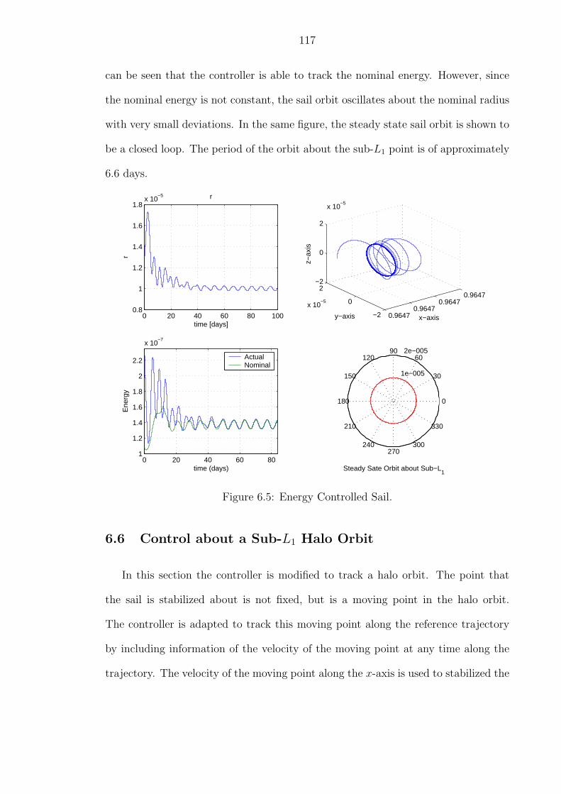
117
can be seen that the controller is able to track the nominal energy. However, since
the nominal energy is not constant, the sail orbit oscillates about the nominal radius
with very small deviations. In the same figure, the steady state sail orbit is shown to
be a closed loop. The period of the orbit about the sub-L1 point is of approximately
6.6 days.
0 20 40 60 80 1000.8
1
1.2
1.4
1.6
1.8x 10
−5 r
time [days]
r
0.96470.9647
0.96470.9647
−2
0
2
x 10−5
−2
0
2
x 10−5
x−axisy−axisz−
axis
0 20 40 60 801
1.2
1.4
1.6
1.8
2
2.2
x 10−7
time (days)
Ene
rgy
ActualNominal
1e−005
2e−005
30
210
60
240
90
270
120
300
150
330
180 0
Steady Sate Orbit about Sub−L1
Figure 6.5: Energy Controlled Sail.
6.6 Control about a Sub-L1 Halo Orbit
In this section the controller is modified to track a halo orbit. The point that
the sail is stabilized about is not fixed, but is a moving point in the halo orbit.
The controller is adapted to track this moving point along the reference trajectory
by including information of the velocity of the moving point at any time along the
trajectory. The velocity of the moving point along the x-axis is used to stabilized the

118
sail at the correct velocity while its x location is being tracked. The velocities of the
moving point, yr and zr, along the y and z axes are used to obtain the kinetic energy
of the moving point Er for controlling the orbiting radius along the trajectory. It is
assumed that the coupling between x-dynamics and y or z dynamics are small and
hence are neglected. With this assumption, the modified version of the controller in
Eq. (6.48) for a moving point is:
α = α1 + c1(x− xr(t)) + c2(x− xr(t)), (6.55)
where xr(t) and xr(t) are the reference position and reference velocity along the
x-coordinate at time t, respectively.
Figure 6.6 depicts the geometry of a sail around a trajectory in the yz-plane. The
modified controller given in Eq. (6.53) for this situation is:
δ = δ − θ − δu, (6.56)
where
tan δ =z − zr
y − yr
, (6.57)
tan θ =z
y, (6.58)
sin δu =Er − E0
k2r0
. (6.59)
Note that when this controller is applied to a fixed equilibrium point it reduces
to the controller developed in the previous section. For an equilibrium point yr and
zr are zero, hence δ and θ are the same. Also the velocity of the equilibrium point is
zero, thus its kinetic energy, Er, is also zero.
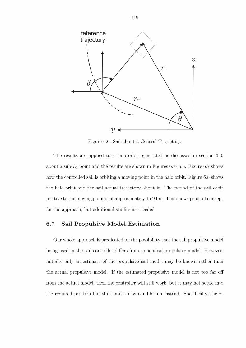
119
d
q
y
z
r
rr
referencetrajectory
Figure 6.6: Sail about a General Trajectory.
The results are applied to a halo orbit, generated as discussed in section 6.3,
about a sub-L1 point and the results are shown in Figures 6.7- 6.8. Figure 6.7 shows
how the controlled sail is orbiting a moving point in the halo orbit. Figure 6.8 shows
the halo orbit and the sail actual trajectory about it. The period of the sail orbit
relative to the moving point is of approximately 15.9 hrs. This shows proof of concept
for the approach, but additional studies are needed.
6.7 Sail Propulsive Model Estimation
Our whole approach is predicated on the possibility that the sail propulsive model
being used in the sail controller differs from some ideal propulsive model. However,
initially only an estimate of the propulsive sail model may be known rather than
the actual propulsive model. If the estimated propulsive model is not too far off
from the actual model, then the controller will still work, but it may not settle into
the required position but shift into a new equilibrium instead. Specifically, the x-

120
0 500 1000 1500 2000−2
−1
0
1
2x 10
4
∆ x [m]
∆ y
[m]
0 500 1000 1500 2000−2
−1
0
1
2x 10
4
∆ x [m]
∆ z
[m]
−2 −1 0 1 2
x 104
−2
−1
0
1
2x 10
4
∆ y [m]
∆ z
[m]
01000
2000
−20
2
x 104
−2
0
2
x 104
∆ x [m]∆ y [m]∆
z [m
]
Figure 6.7: Relative sail orbit with respect to moving point on halo orbit. Time ofpropagation is 3.65 days.
1.44321.4432
1.44321.4432
1.4432
x 1011
−2
−1
0
1
2
x 106
−1
−0.5
0
0.5
1
x 108
x−axis [m]y−axis [m]
z−ax
is [m
]
ReferenceActual
Figure 6.8: Controlled sail about Halo Orbit about sub-L1 point.

121
position will be affected by the uncertainty in the propulsive model. For simplicity, it
is assumed that the sail is desired to be stationed at a sub-L1 point using the above
methodology. Using the difference between the new equilibrium and the required sub-
L1 point it is possible to refine the estimate of the propulsive model. For achieving
this, a formalism for updating the propulsive parameters can be obtained from the
control laws. The objective is to find the sensitivity of changes in the x-equilibrium
with respect to changes in the propulsive model, which for the ideal sail is the k
parameter. This sensitivity can be written as:
∂x
∂k=
∂x
∂α
∂α
∂k, (6.60)
each of the partial derivatives in the right-hand side of the equation can be computed
from the control laws, Eqs. (6.48)-(6.49). Note that α is time varying, nonetheless,
an average value can be used to approximate the partial derivative. Thus, from the
average value of α in Eq. (6.49), the partial derivative of α with respect to k is
∂α
∂k= −
[xL1 −
(1− µ)(xL1 + µ)
|r1(xL1)|3− µ
|r2(xL1)|3(xL1
+ µ− 1)]|r1(xL1)|2β(1− µ)
· 1
k23 cos2 α sin α, (6.61)
the other partial derivative, obtained from Eq. (6.48), is simply
∂x
∂α=
1
c1
. (6.62)
Thus, once the sail settles into a constant or nearly constant distance from the
sun along the x-direction, the difference between the current and desired position
can be used to update k through:

122
∆k ≈ ∆x
∂x/∂k. (6.63)
Several iterations are in general necessary before converging into the the actual
value of k. This current approach shows the feasibility of an estimation method and
is not optimal in general.
Figure 6.9 shows the application of this idea to two cases. In the first case the
controller assumes a k = 1.1 while the actual is 1.05 and the sail is starts behind
the sub-L1 point at a distance of 2 × 10⁻⁵, in the normalized units. In the second
case the actual k is 1.15 and the controller is initialized with k = 1.1 with the sail
initially located at the same distance as the first case but sunward of the sub-L1
point. In both of these cases, the controller tries to stabilize the sail x-position.
When the controller senses that it is converging to a different x-location, it uses this
information to update k. After 120 days, k = 1.0493 and k = 1.1506 for the first
and second cases, respectively.
The estimation can also be done with the second PD-controller presented and
shown by the simulation in figure 6.10. The same two above cases for the imple-
mentation of the adaptive controller were used. The sail was placed at distance of
2×10⁻⁵, in the normalized units, sunward and behind of xL1 . During the simulation,
the k parameter is estimated to a value close to the actual, however, since the sail
x-position does not settle into a constant value, the estimation is not perfect and the
k parameter does not converge exactly. Despite this, the sail is driven close to the
desired location with this control implementation.

123
0 50 100 150−3
−2
−1
0
1
2x 10
−5 ∆ x vs. time. k=1.15
time [days]
∆ x
1e−005
2e−005
30
210
60
240
90
270
120
300
150
330
180 0
Steady State Orbit about Sub−L1.k=1.15
0 50 100 150−3
−2
−1
0
1
2
3x 10
−5 ∆ x vs. time. k=1.05
time [days]
∆ x
1e−005
2e−005
30
210
60
240
90
270
120
300
150
330
180 0
Steady State Orbit about Sub−L1. k=1.05
Figure 6.9: Adaptive controller.
6.8 Sail Control Under Degradation
The sail membrane will suffer from degradation due to solar radiation and the
space environment [20]. The membrane degradation will result in a loss of propulsion
forces acting on the sail. In order to maintain the sail orbiting the sub-L1 point this
effect must be accounted for in E0. It is possible to keep a constant radius about
the equilibrium, however, this control law would fail when the force acting on the
sail becomes insufficient for maintaining the x-position of the equilibrium. A better
approach is to make the radius decrease as the sail degrades. Hence, the sail will
eventually settle into the sub-L1 point when the sail performance degrades to its
minimum at β′ = β. For such approach, the required energy satisfies:

124
0 50 100 150−3
−2
−1
0
1
2
3x 10
−5 ∆ x vs. time. k=1.05
time [days]
∆ x
1e−005
2e−005
30
210
60
240
90
270
120
300
150
330
180 0
Steady State Orbit about Sub−L1. k=1.05
0 50 100 150−3
−2
−1
0
1
2x 10
−5 ∆ x vs. time. k=1.15
time [days]
∆ x
1e−005
2e−005
30
210
60
240
90
270
120
300
150
330
180 0
Steady State Orbit about Sub−L1. k=1.15
Figure 6.10: Adaptive controller for the simple PD-Controller.
E0 =1
2r2dθ
2 =1
2r2d0k
2θ2, (6.64)
where k is a function of time, and the orbit radius satisfies rd(k(0)) = rdo (the initial
value of the orbit radius) and rd(1) = 0. It is possible to choose how rd changes with
degradation. For instance, if rd varies linearly with k, then:
E0 =1
2
(k(t)− 1
k(0)− 1
)2
r2d0θ
2, (6.65)
where k(t) is the value of k at time t, and k(0) is the initial value of k. When k = 1,
the sail radius is zero and the sail is at the sub-L1 point at which the reference energy

125
is zero. When k(t) < 1, the sail force is not sufficient to keep it at the equilibrium
and a mission redesign must occur. Figure 6.11 shows a simulation of a solar sail
under degradation. The sail was initially positioned sunward of the equilibrium. The
controller stabilized the sail at the required x-position and the radius was decreased
as the sail surface degraded.
1e−005
2e−005
30
210
60
240
90
270
120
300
150
330
180 0
Sail Radius
0.9647
0.9647
0.9647
0.9647
−2
−1
0
1
2
x 10−5
−1.5
−1
−0.5
0
0.5
1
1.5
2
x 10−5
x−axisy−axis
z−ax
is
Figure 6.11: Solar sail under degradation.
A final test is now given which involves simultaneous control, estimation, and
degradation of the sail. Here the sail is considered to undergo surface degradation
and at the same time we try to estimate its value to be used in the controller.
Initially, the sail is located 2 × 10⁻⁵ distance units sunward of the equilibrium and
with a larger radius than the nominal. For simulation purposes, the sail degrades
linearly with time. Initially, the actual value of β′ is 0.115 or k(0) = 1.15. The initial
estimate of k used in the controller is 1.1. After 150 days k decays to 1.0897 while the

126
estimated value is 1.092. Initially the sail overshoots xL1 , but as the estimation of
k becomes closer to the actual value the sail approaches the equilibrium’s x-position
while the orbiting radius is reduced as the sail propulsion decays. Figure 6.12 shows
a simulation of the sail trajectory for this case.
2e−005
4e−005
30
210
60
240
90
270
120
300
150
330
180 0
0.9647
0.9647
0.9647
0.9647
−4
−2
0
2
4
x 10−5
−3
−2
−1
0
1
2
3
x 10−5
x−axisy−axis
z−ax
is
Figure 6.12: Solar Sail Under Degradation and Uncertainties.
6.9 Control Implementation
So far in our discussion, we have neglected the actual implementation of control
laws in the sail environment. We now show, through explicit discussion, that our
methodology can be implemented into a standard sail design.
There are two ways in which the controller can be implemented. The sail can be
made to spin with an average angular velocity and use the attitude control system to
modulate the angular velocity needed to follow the nominal orbit. Thus, one of the
sail body fixed axis is always pointing outward from the equilibrium point. In this

127
case we choose the sail Y body-fixed axis to point away from the center of the sub-L1
relative orbit. The angle α is controlled by exerting moments about the sail X-axis
while δ is controlled by rotating the about sun-sail line. Another option is to change
the sail attitude at every point in the orbit without exerting any moments about
the sail normal axis. For this approach, α and δ are effected by a combination of
moments about the sail X and Y body-fixed axes. Both of these approaches control
the angle α and δ to keep the sail in a quasi-circular orbit. In this paper we only
consider the spinning case and we assumed that the sail behaves as a rigid body with
moments of inertia axes coincident with the sail body-fixed axes.
The dynamics for a spinning rigid body are governed by Euler equations. Given
a set of required angular velocities and their rates, the torques needed to achieved
them are given by:
MX = IX ωX + (IZ − IY )ωY ωZ , (6.66)
MY = IY ωY + (IX − IZ)ωXωZ , (6.67)
MZ = IZωZ + (IY − IX)ωXωY , (6.68)
Where Mi, Ii, and ωi are a moment, a moment of inertia, and an angular velocity
about the sail body-fixed i-axis, respectively. We assume that the sail Z-axis is
coincident with the sail normal and that IZ is the sail maximum moment of inertia.
The angular velocities, in the sail body-fixed frame and with the sail Y body-fixed
axis pointing outward from the sub-L1 equilibrium point, can be obtained from the
sail angle rates:

128
ωX = δ sin α, (6.69)
ωY = α, (6.70)
ωZ = −δ cos α. (6.71)
Recall that δ = θ + δ. The angular rates are obtained from the controller com-
mands and must be in radians per second. Taking a time derivative yields
ωX = δ sin α + δα cos α, (6.72)
ωY = α, (6.73)
ωZ = −δ cos α− δα sin α. (6.74)
For a general sail, the moments needed are:
MX = IX(δ sin α + δα cos α)− (IZ − IY )αδ cos α, (6.75)
MY = IY α− (IX − IZ)δ2 cos α sin α, (6.76)
MY = −IZ(δ cos α− δα sin α) + (IY − IX)αδ sin α. (6.77)
These are the moments that need to be supplied to the sail by the attitude control
system in order to follow the control commands. The moments can be generated by
having control vanes [34], movable sail quadrants, or any other type of attitude
control [34, 35]. Figure 6.13 shows the moments required to maintain the sail for the
Solar Polar Imager mission (SPI) [36] in a circular orbit about a sub-L1 point. The
mass of the sail is 450 kg and its principal moments of inertia are 321490 kg m2,
321490 kg m2, and 642876 kg m2, along the X, Y , and Z axes[36], respectively.
For a sun-sail-line angle α that is almost constant, such as is the case of the last
PD-controller developed, it can be assumed that α = 0 and α = 0. Then, the control
torques needed for the spinning the sail simplify to:

129
0 20 40 60 80 100−5
0
5x 10
−6
My
[Nm
]
time [days]
0 20 40 60 80 100−1
0
1x 10
−5
Mz
[Nm
]
time [days]
0 20 40 60 80 100−1
0
1x 10
−9
Mx
[Nm
]time [days]
Figure 6.13: Control moments required for station-keeping SPI sail.
MX = IX δ sin α, (6.78)
MY = −(IX − IZ)δ2 cos α sin α, (6.79)
MZ = −IZ δ cos α. (6.80)
When the sail reaches steady-state δ → 0 and δ → constant. Thus the steady
state moments are:
MX = 0, (6.81)
MY ≈ constant, (6.82)
MZ = 0. (6.83)
Thus, the long term control of the sail attitude is effected by applying a constant

130
torque about the sail y-axis, which point away from the orbit center. Specific imple-
mentation of such control laws are not considered in this paper, but can be found in
References [34, 35] and [22].

CHAPTER VII
Conclusions
This dissertation studies the modeling of solar sails of arbitrary shape, the es-
timation of force and moment coefficients based on navigation data, and trajectory
control. The goal is to develop an analytic methodology to capture all the features
present in a solar sail surface to accurately describe the force and moment generated
by the sail as they are highly dependent in the sail shape. Having a precise analytic
model of a solar sail is advantageous over a finite element model as the first can be
easily incorporated in existing navigation tools. We achieve this objective by deriving
the generalized solar sail model (GSM), which captures the force and moment acting
on a solar sail of general shape using a series of tensors defined as surface integrals.
Once the GSM is defined, it is used to compare the performance of different sail
geometries. Also, since both the force and moment acting on a solar sail are linear
in the GSM coefficients, the GSM is used to develop a linear-estimation algorithm
from navigation or tested data. Then, robust control laws are developed using the
ideal sail model. These control laws are used to station a solar sail at a sub-L1 point
or to track a halo orbit in the vicinity of a sub-L1 point. Detailed results and future
topics of research are given in the following sections.
131

132
7.1 Main Results in this Dissertation
In Chapter II, the dynamics of both the restricted two-body problem and the
circular restricted three-body problem were presented. Then, a brief derivation of
the models for the sun’s solar radiation pressure were given, which is the source of the
force and moments experienced by the sail. Next, the classical flat solar sail models
were presented for the ideal and non-ideal cases. The flat sail models are useful
during initial mission design studies, however, a more precise model is necessary for
a final mission trajectory and actual sail navigation.
In Chapter III, an analytic model for solar sails of arbitrary shape is developed.
Equations for the force and moment are derived in terms of tensors, which are in-
dependent of the sail attitude. Thus, the resulting equations can be used in all
orientations of the sail. With the force and moment defined, it is shown how the
center of pressure can be calculated. It is shown that solar sails with symmetries in
their geometries require fewer coefficients for capturing the force and moment. The
number of independent parameters needed depends on the type of symmetry.
In Chapter IV, applications of the GSM to several examples are presented. Four
sails with different geometries are presented. It is shown how the force and moment
tensor are computed for each of these sails once their specific shape is defined. Then,
the force and moment generated by these sails are compared and their differences are
pointed out. Also, first and second order force partial derivatives are presented. The
analytic nature of the GSM equations allows the derivation of partial derivatives,
which are required in optimization algorithms and in other studies. It is also shown
that the GSM equations can be used in previous studies where the flat sail models had
been used before. Specifically, a guidance law and attitude for maximum propulsive

133
force are developed for a square, billow sail. Finally, NASA’s S5 project is discussed,
as well as how the GSM equations form a central part in this software package.
In Chapter V, an estimation algorithm for the GSM force and moment coefficients
is developed. The force and moment equations are linear in the tensors coefficients,
which are manipulated into a product of a matrix and vector to facilitate the es-
timation. It is shown that the accuracy of the estimation results is dependent on
the attitudes at which the measurements are taken. Several attitude samplings are
discussed and their effect on the covariances of the estimates is also discussed. The
simulated data used in the estimation examples are generated with a sinusoid sail.
In Chapter VI, the solar sail ideal flat model is used to develop control laws
to station a sail about a sub-L1 point or to track a neighboring halo orbit. The
equations of motion of the circular restricted three-body problem and the equations
for the sail propulsion are transformed into cylindrical coordinates to develop the
controllers. Control of the sail location along the x-axis and control of the sail orbit
about the equilibrium point require two independent controllers. A linear feedback
controller and a proportional-derivative controller are developed to control the sail
distance from the sun. An energy-based feedback controller is presented to control
the sail orbit about the chosen equilibrium point. These controllers are modified to
place the sail about a halo orbit. A simple adaptive control technique is used to
estimate the sail performance when the sail optical parameters degrade.
The results presented in this dissertation open a new way of modeling and flying
solar sails. Modeling forces and moments on solar sails are no longer restricted to
simple analytical sail models or finite-element models. The generalized sail model
introduces a new way of modeling solar sails and estimating parameters from navi-
gation data. Excess thrust controllers allow the tracking of nominal trajectories for

134
sail with higher performance that the mission requires.
7.2 Future Research
Several of the topics presented in this dissertation can be expanded, and should
be studied further in the future. A list of topics include:
1. Analysis of sail shapes varying with solar sail attitude.
In this dissertation, the generalized sail model equations were developed under
the assumption that the sail shape remains constant with sail attitude. It is
known that the sail shape is dependent on the sail attitude, however, no data
exists on the magnitude of the deformations. Also, due to the lightweight and
extended sail structure the sail may have oscillating modes that will affect the
sail shape. Further studies should be made when more data on this is available.
2. Studies of the effect of sail self-shadowing on sail performance.
Another assumption in this dissertation is that all of the sail surface is illu-
minated all the time. A situation that may invalidate this assumption are
billowed sails at high α angles. Another more common situation is when the
sail attitude control system uses an articulated boom with a mass to change
the sail center of mass and generate a torque. When the boom is moved to
change the center of mass, part of the sail will have a shadow over it. Also, the
shadow cast on the sail surface will be time varying.
3. Refinement of the trajectory control laws.
In this dissertation several controllers were developed using the ideal flat sail
model. However, GSM allows to obtain more accurate control laws, which take
into account the sail shape. Further research on developing controller using

135
GSM should be performed. Also, the control laws developed for tracking a
halo orbit require further studies to achieve a reasonable rotation rate about
the moving point in the halo orbit.

APPENDIX A
S5 MATLAB SOLAR RADIATION PRESSURE
The following Matlabr code was used in the development of the the Solar Radia-
tion Pressure module of the S5 project. The main program that calculates the total
force and moment acting on a solar sail, due to the sail itself and control vanes, is
first presented. Then, the auxiliary subroutines necessary are also presented.
A.1 Force and Moment
function [F,T]=srp(psi,q,r1,flag)
global a2 a3 rho s
%Reading Sail Properties load prop.dat
%Sail Parameters
%Optical Parameters
rho=prop(1); %Reflectivity
s=prop(2); %Fraction of specular Reflection
Bf=prop(3); %Front Surf. Non-Lambertian Coefficient
Bb=prop(4); %Back Surf. Non-Lambertian Coefficient
emb=prop(5); %Back Emissivity
emf=prop(6); %Front Emissivity
136

137
As=prop(7); %Sail Area [m2]
va=prop(8); %Vane Area
momarm=prop(9); %Moment Arm
a2=Bf*(1-s)*rho+(1-rho)*(emf*Bf-emb*Bb)/(emf+emb);
a3=1-rho*s;
% Loading sail GSM Force and Moment Tensors
load coefs06.mat
%Matrix Transformation
%Inertial To Body-Fixed Frame
R=quaternion(q); % Subroutine
% Solar Pressure
r=norm(r1);
P=solp(r);
r0=R*r1/r;
% Location of Vanes CP in Body-Fixed Frame
arm=momarm*[1 0 -1 0; 0 1 0 -1; 0 0 0 0];
if flag <= 2
%Coordinates of Vane Normal Vectors
%in Sail Body-Fixed Frame
Rv=vanenorm(psi); % Subroutine
%Calling localcoord m-file for
%Calculation of normal and tangential vectors
[n,t]=localcoord(R,r1,Rv); % Subroutine
for i=1:5
%Calculation of Normal-to-Sun-Line angle

138
%for sail and control vanes
alpha(i)=acos(-dot(n(:,i)’,r1)/r);
%Forces on sail
%Force: Normal Component
if (i==1)
A=As;
else
A=va;
end
%Force: Normal Component
Fn(i)=-P*A*((1+rho*s)*(cos(alpha(i)))∧2+Bf*(1-s)*rho*cos(alpha(i))+
(1-rho)*(emf*Bf-emb*Bb)/(emf+emb)*cos(alpha(i)));
%Force: Tangential Component
Ft(i)=P*A*(1-rho*s)*cos(alpha(i))*sin(alpha(i));
%Resultant Force in Inertial Frame. Force in Newtons
fm(:,i)=Fn(i)*n(:,i)+Ft(i)*t(:,i);
end
%Total Force in Inertial frame
Fbf=R*fm;
if flag == 1
F=sum(fm’)’;
elseif flag == 2
%Forces in Sail-Body-Fixed
F=sum(Fbf’)’;
end

139
%Calculation of torques
for i=1:4
k=1+i;
tor(:,i)=cross(arm(:,i),
Fbf(:,k));
end
T=sum(tor’)’;
elseif flag >=3
f1=-a3*dot(J1,r0)*r0;
f2=a2*dr2(J2,r0);
f3=-2*rho*s*dr3d(J3,r0);
F1=P*(f1+f2+f3);
[Fv, Mv]=FTvanes(psi,r0); % Subroutine
Fv=P*Fv; F2=sum(Fv’)’;
Fbf=F1+F2;
if flag==3
F=R’*Fbf;
elseif flag==4
F=Fbf;
end
%Calculation of Sail Internal Torque
m1=a2*dr2(K2,r0);
m2=-2*rho*s*dr3d(K3,r0);
m3=-a3*cross(dr2b(L,r0),r0);
M=P*(m1+m2+m3);
140
Mv=P*sum(Mv’)’;
for i=1:4
tor(:,i)=cross(arm(:,i),
Fv(:,i));
end
T1=sum(tor’)’;
T=M+Mv+T1;
end
A.2 Vanes Normal Vectors in the Sail-Body Fixed Frame
function vnor= vanenorm (psi)
% This routine uses the vane defection angles ,psi, with respect
% to the sail to calculate the normal vector of each vane for the
% case of a flat vanes.
zva=[0 0 1];
%Rotation about X. Vane 1
R1=[1 0 0; 0 cos(psi(1)) sin(psi(1)); 0 -sin(psi(1)) cos(psi(1))]’*zva;
%Rotation about Y. Vane 2
R2=[cos(psi(2)) 0 -sin(psi(2)); 0 1 0; sin(psi(2)) 0 cos(psi(2))]’*zva;
%Rotation about X. Vane 3
R3=[1 0 0; 0 cos(-psi(3)) sin(-psi(3)); 0 -sin(-psi(3)) cos(-psi(3))]’*zva;
%Rotation about Y. Vane 4
R4=[cos(-psi(4)) 0 -sin(-psi(4)); 0 1 0; sin(-psi(4)) 0 cos(-psi(4))]’*zva;
vnor=[R1 R2 R3 R4];

141
A.3 Force and Moment due to Control Vanes
function [Fv, Mv]=FTvanes(psi,r0)
%This File computes the force and moment
%for each of the sail vanes given their angular
% deflection with respect to the sail, which is in terms
%in the vector psi=[psi(1), psi(2), psi(3), psi(4)]
global a2 a3 rho s
load coefv06.mat
%Rotation about X. Vane 1
R1=[1 0 0; 0 cos(psi(1)) sin(psi(1)); 0 -sin(psi(1)) cos(psi(1))];
%Rotation about Y. Vane 2
R2=[cos(psi(2)) 0 -sin(psi(2)); 0 1 0; sin(psi(2)) 0 cos(psi(2))];
%Rotation about X. Vane 3
R3=[1 0 0; 0 cos(-psi(3)) sin(-psi(3)); 0 -sin(-psi(3)) cos(-psi(3))];
%Rotation about Y. Vane 4
R4=[cos(-psi(4)) 0 -sin(-psi(4)); 0 1 0; sin(-psi(4)) 0 cos(-psi(4))];
for i=1:4
%Rotation about Z-BFF axis to account
%for vane-sail axis alignments
ang=(i-2)*pi/2;
Rz=[cos(ang) sin(ang) 0 -sin(ang) cos(ang) 0 0 0 1];
if i==1
%Force and Torque on Vane 1
rv1=Rz*R1*r0;

142
fv1=-a3*dot(Jv1,rv1)*rv1;
fv2=a2*dr2(Jv2,rv1);
fv3=-2*rho*s*dr3d(Jv3,rv1);
Fv1vff=fv1+fv2+fv3;
Fv1=R1’*Rz’*Fv1vff;
mv1=a2*dr2(Kv2,r0);
mv2=-2*rho*s*dr3d(Kv3,r0);
mv3=-a3*cross(dr2b(Lv,r0),r0);
Mv1vff=(mv1+mv2+mv3);
Mv1=R1’*Rz’*Mv1vff;
elseif i==2
%Force and Torque on Vane 2
rv2=Rz*R2*r0;
fv1=-a3*dot(Jv1,rv2)*rv2;
fv2=a2*dr2(Jv2,rv2);
fv3=-2*rho*s*dr3d(Jv3,rv2);
Fv2vff=fv1+fv2+fv3;
Fv2=R2’*Rz’*Fv2vff;
mv1=a2*dr2(Kv2,r0);
mv2=-2*rho*s*dr3d(Kv3,r0);
mv3=-a3*cross(dr2b(Lv,r0),r0);
Mv2vff=(mv1+mv2+mv3);
Mv2=R2’*Rz’*Mv2vff;
elseif i==3
%Force and Torque on Vane 3

143
rv3=Rz*R3*r0;
fv1=-a3*dot(Jv1,rv3)*rv3;
fv2=a2*dr2(Jv2,rv3);
fv3=-2*rho*s*dr3d(Jv3,rv3);
Fv3vff=fv1+fv2+fv3;
Fv3=R3’*Rz’*Fv3vff;
mv1=a2*dr2(Kv2,r0);
mv2=-2*rho*s*dr3d(Kv3,r0);
mv3=-a3*cross(dr2b(Lv,r0),r0);
Mv3vff=(mv1+mv2+mv3);;
Mv3=R1’*Rz’*Mv3vff;
elseif i==4
%Force on Vane 1
rv4=Rz*R4*r0;
fv1=-a3*dot(Jv1,rv4)*rv4;
fv2=a2*dr2(Jv2,rv4);
fv3=-2*rho*s*dr3d(Jv3,rv4);
Fv4vff=fv1+fv2+fv3;
Fv4=R4’*Rz’*Fv4vff;
mv1=a2*dr2(Kv2,r0);
mv2=-2*rho*s*dr3d(Kv3,r0);
mv3=-a3*cross(dr2b(Lv,r0),r0);
Mv4vff=(mv1+mv2+mv3);;
Mv4=R1’*Rz’*Mv4vff;
end

144
end
%Total force produced by vanes
Fv=[Fv1 Fv2 Fv3 Fv4];
%Total moment produced by vanes
Mv=[Mv1 Mv2 Mv3 Mv4];
A.4 Normal and Transverse Vectors
function [n,t] = localcoord(R,r,Rv)
% This file computes the sail normal and transverse
% vectors given a rotation matrix R that transforms
% the sail inertial coordinates into a body-fixed, the
% sail position vector r, and the the matrix Rv, which contains
% the the vanes’ normal vectors
n1=[R(3,1) R(3,2) R(3,3)]’;
R2=R’*Rv; n2=[n1 R2];
r1=r/norm(r);
%Computing Tangential vector in Inertial Coordinates
for i=1:5
n(:,i)=n2(:,i)/norm(n2(:,i));
om1=cross(n(:,i)’,r1);
if (norm(om1)==0)
t(:,i)=[1 0 0]’;
else om=om1/norm(om1);
t(:,i)=cross(om,n(:,i))’;
end

145
end
A.5 Sail Attitude
function [R] = quaternion(q)
% This code take the sail attitude information in quaternion
% and returns a a rotation matrix R from inertial to sail
% body fixed coordinates
q0=[q(1); q(2); q(3)];
S=[0 -q(3) q(2); q(3) 0 -q(1); -q(2) q(1) 0];
%Transformation of quaternion to inertial-to-body-fixed
%Rotation Matrix
R=(q(4)∧2-q0’*q0)*eye(3)+2.*q0*q0’-2.*q(4)*S;
A.6 Solar Radiation Pressure
function p= solp(r)
% This program computes the sun’s solar radiation
% pressure , p, at a distance r form the sun
%Reading Physical Constants
load physconst.dat
%Natural Parameters
Rs=physconst(1); %Sun Radius (m)
Io=physconst(2); %Sun’s Specific Intensity (W/m∧2)
c=physconst(3); %Speed of Light (m/s)
% Solar Pressure
%Takes into account Solar disk

146
Fr=2/3.*(r/Rs).∧2.*(1-(1-(Rs./r).∧2).∧(3/2));
Pr=1/c*Io*pi.*(Rs./r).∧2;
p=Pr.*Fr;

BIBLIOGRAPHY
[1] H. Baoyin and C.R. McInnes. Solar sail halo orbits at the sun-earth artificial l1point. Celestial Mechanics and Dymanical Astronomy, 2006(94):155–171, 2006.
[2] B. Dachwald. Optimal solar-sail trajectories for missions to the outer solarsystem. Journal of Guidance, Control, and Dynamics, 28(6):1187–1193, 2005.
[3] B. Dachwald. Solar sail trajectory optimization for intercepting, impacting, anddeflecting near-earth asteroids. In AIAA Guidance, Navigation, and ControlConference and Exhibit, August 15-18, 2005. San Francisco, CA.
[4] J.M.A. Danby. Fundamentals of Celestial Mechanics. Willmann-Bell, Inc.,Richmond, VA, 1992.
[5] B. Derbes and D. Lichodziejewski. Sail coordinate systems and format for re-porting propulsive perfomance. In The 14th AAS/AIAA Space Flight MechanicsMeeting, February 8-12, 2004. Maui, Hawaii.
[6] B. Derbes and G. Veal. Team encounter solar sails. In The 45thAIAA/ASME/ASCE/AHS/ASC Structures, Structural Dynamics and Materi-als Conference, April 19-22, 2004. Palm Springs, California.
[7] J. Ellis, Lisano M., P. Wolff, J. Evans, J. Bladt, D.J. Scheeres, L. Rios-Reyes, andD. Lawrence. A solar sail integrated simulation toolkit. In The 14th AAS/AIAASpace Flight Mechanics Meeting, February 8-12, 2004. Maui, Hawaii.
[8] C. Garner and M. Leipold. Developments and activities in solar sail propulsion.In 36th AIAA/ASME/SAE/ASEE Joint Propulsion Conference and Exhibit,July 16-19, 2000. Huntsville, Alabama.
[9] V.M. Gotlib, et. al. Cosmos 1: The worlds first solar sail spacecraft. In The14th AAS/AIAA Space Flight Mechanics Meeting, February 8-12, 2004. Maui,Hawaii.
[10] D.T. Greenwood. Principles of Dynamics. Prentice Hall, New Jersey, 1988.
[11] R.J. Hale. Introduction to Space Flight. Prentice Hall, New Jersey, 1994.
[12] A.F. Heaton. Solar sail gnc model comparisons. In AIAA Guidance, Navigation,and Control Conference and Exhibit, 2004. Providence, Rhode Island.
147

148
[13] K.R. Koch. Parameter Estimation and hypothesis Testing in Linear Models.Springer, New York, 1999.
[14] R.E. Larson, R.P. Hostetler, and B.H. Edwards. Calculus with Analytic Geom-etry.
[15] D.A. Lawrence and S.W. Piggott. Integrated trajectory and attitude control fora four-vane solar sail. In AIAA Guidance, Navigation, and Control Conferenceand Exhibit, August 15-18, 2005. San Francisco, CA.
[16] D.A. Lawrence and S.W. Piggott. Solar sail trajectory control for sub-l1 station-keeping. In AIAA Guidance, Navigation, and Control Conference and Exhibit,August 16-19, 2004. Providence, RI.
[17] D. Lichodziejewski, B. Derbes, K. Belvin, K. Slade, and T. Mann. Developmentand ground testing of a compactly stowed scalable inflatably deployed solar sail.In The 45th AIAA/ASME/ASCE/AHS/ASC Structures, Structural Dynamicsand Materials Conference, April 19-22, 2004. Palm Springs, California.
[18] D. Lichodziejewski, B. Derbes, K. Slade, and T. Mann. Vacuum deploymentand testing of a 4-quadrant scalable inflatable rigidizable solar sail system. InThe 46th AIAA/ASME/ASCE/AHS/ASC Structures, Structural Dynamics andMaterials Conference, April 18-21, 2005. Austin, Texas.
[19] M. Lisano, D. Lawrence, and S. Piggot. Solar sail transfer trajectory designand stationkeeping control for missions to the sub-l1 equilibrium region. In15th AAS/AIAA Space Flight Mechanics Meeting, January 23-27, 2005. CopperMountain, Colorado.
[20] F. Lura and D. Hagelschuer. Experiments in the test facility kobe for the in-vestigation of degradation effects of thin foil samples for a solar sail missionconcerning the simultaneous influence of space environment properties. In 22ndSpace Simulation Conference, 2002. Ellicott City, MD.
[21] C.R. McInnes. Solar Sailing: Technology, Dynamics and Mission Applications.Springer-Praxis, Chichester, UK, 1999.
[22] E. Mettler and Ploen S.R. Solar sail dynamics and control using a boommounted bus articulated by a bi-state two-axis gimbal and reaction wheels.In AIAA/AAS Astyrodynamics Specialist Conference and Exhibit, 5-8 August2002. Monterrey, California.
[23] J.R. Meyer-Arendt. Introduction to Classical and Modern Optics. Prentice Hall,New Jersey, 1989.
[24] O.M. Mori, Y. Tsuda, M. Shida, and J. Kawaguchi. Dynamic and static de-ployment motions of spin type solar sail. In The 18th International Symposiumon Space Flight Dynamics, October 11-15, 2004. Munich, Germany.

149
[25] D.M. Murphy and B.D. Macy. Demonstration of a 10-m solar sail system. InThe 45th AIAA/ASME/ASCE/AHS/ASC Structures, Structural Dynamics andMaterials Conference, April 19-22, 2004. Palm Springs, California.
[26] L. Rios-Reyes and D.J. Scheeres. Applications of the generalized model for solarsails. In AIAA Guidance, Navigation, and Control Conference and Exhibit,2004. Providence, Rhode Island.
[27] L. Rios-Reyes and D.J. Scheeres. Generalized model for solar sails. Journal ofSpacecraft and Rockets, 42(1):182–285, 2005.
[28] L. Rios-Reyes and D.J. Scheeres. Robust solar sail trajectory control for largepre-launch modeling errors. In AIAA Guidance, Navigation, and Control Con-ference, August 15-18, 2005. San Francisco, CA.
[29] L. Rios-Reyes and D.J. Scheeres. Generalized models for solar sails. In The14th AAS/AIAA Space Flight Mechanics Meeting, February 8-12, 2004. Maui,Hawaii.
[30] L. Rios-Reyes and D.J. Scheeres. Solar sail navigation: Estimation of force, mo-ment, and optical parameters. In The 16th AAS/AIAA Space Flight MechanicsMeeting, January 22-26, 2006. Tampa, FL.
[31] L. Rios-Reyes and D.J. Scheeres. Solar sail navigation with the generalized sailmodel. In The 15th Workshop on JAXA Astrodynamics and Flight Mechanics,,July 25-26, 2005. ISAS/Jaxa, Japan.
[32] D.N. Sharma and D.J. Scheeres. Solar system escape trajectories using solarsails. Journal of Spacecraft and Rockets, 41(4):684–687, 2004.
[33] S. Takeuchi. Deployment experiment result of solar sail using sounding rocket.In 55th International Astronautical Congress of the International AstronauticalFederation, the International Academy of Astronautics, and the InternationalInstitute of Space Law, October 4-8, 2004. Vancouver, Canada.
[34] B. Wie. Solar sail attitude control and dynamics, part 1. Journal of Guidance,Control, and Dynamics, 27(4):526–535, 2004.
[35] B. Wie. Solar sail attitude control and dynamics, part 2. Journal of Guidance,Control, and Dynamics, 27(4):536–544, 2004.
[36] B. Wie and D. Murphy. Propellantless aocs design for a 160-m, 450-kg sailcraftof the solar polar imager mission. In 41st AIAA Joint Propulsion Conference,July 10-13, 2005. Tucson, AZ.
[37] J.L. Wright. Space Sailing. Gordon and Breach Science Publishers, Philadel-phia, Pennsylvania, 1992.
[38] J.L. Wright and J. Warmke. Solar sail mission applications. In AIAA/ASSAstrodynamics Conference, August 18-20, 1976. San Diego, CA.


![Solar Sails[1]](https://static.fdocuments.us/doc/165x107/577d22ae1a28ab4e1e97fcd0/solar-sails1.jpg)