Soil Resistance Predictions From Pile Dynamics. Current Practices and Future Trends in Deep...

8/2/2019 Soil Resistance Predictions From Pile Dynamics. Current Practices and Future Trends in Deep Foundations

http://slidepdf.com/reader/full/soil-resistance-predictions-from-pile-dynamics-current-practices-and-future 1/23

SOIL RESISTANCE PREDICTIONS FROM PILE DYNAMICS

By Frank Rausche,1 Fred Moses,2 A.M. ASCE and George G. Goble,3 M. ASCE

This paper was originally published in the September, 1972, issue of the Journal of the Soil Mechanics and Foundations Division, ASCE. It is reprinted here with the permission of ASCE

ABSTRACT: An automated prediction scheme is presented which utilizes both forceand acceleration records measured at the pile top during driving to compute the soilresistance forces acting along the pile. The distribution of these forces is determined,and the dynamic and static resistance forces are distinguished such that a predictionof a theoretical static load versus penetration curve is possible. As a theoretical basisstress wave theory is used, derived from the general solution of the linear one-dimensional wave equation. As a means of calculating the dynamic pile response, alumped mass pile model is devised and solved by the Newmark β -method. Wavetheory is also employed to develop a simple method for computing static bearingcapacity from acceleration and force measurements. Twenty-four pile tests arereported, 14 of them with special instrumentation, i.e., strain gages along the pile below grade. The piles tested were of 12-in. (30-cm) diameter steel pipe with lengthsranging from 33 ft. to 83 ft. (10 m to 25 m).

INTRODUCTION

Observations made during impact driving are widely used to predict the static bearing capacity of piles. The results often do not agree with static load tests due to alack of knowledge of hammer energy, cushion characteristics, set per blow and other factors. Recent developments in electronics have made it possible to make accuraterecords of force and acceleration at the pile top during impact driving. Such records,

1 Asst. Prof. of Engrg., Case Western Reserve Univ., Cleveland, Ohio.2 Assoc. Prof. of Engrg., Case Western Reserve Univ., Cleveland, Ohio. 3 Prof. of Civ. Engrg., Case Western Reserve Univ., Cleveland, Ohio.



2

which last only a matter of milliseconds, will be used herein to predict soil resistanceeffects on the pile. Previous work done on this project by a group at Case WesternReserve University reported the use of force and acceleration records in a simplifiedmodel to predict static bearing capacity (4, 5, 6, 11). These results were based onimpact records which were taken after a setup period so that strength changes due to

soil remolding or porewater pressure dissipation were included.The present work extends the application of the force and acceleration records tothe calculation of the distribution of soil resistance along the pile. It also shows howthe records are used to predict the magnitude of dynamic resistance that the soilapplies to the pile, an important factor in choosing efficient hammer characteristics. Amethod for obtaining a more accurate simplified prediction of total static bearingcapacity is also presented. It should be emphasized that the aforementioned predictions are all made from measurements at the pile top only. The work iscorrelated by presentation of results for 24 pile tests which include construction staticload tests as well as specially instrumented load test piles.

The application of these results can have considerable impact on foundation costs.

Static load tests are very costly and time consuming. In Ohio a single test on a service pile using tension reaction piles (also service piles) typically costs $3,000 to $5,000.This static test provides much useful information about the particular pile which wastested. However, due to variability of soil properties the information may be of lessvalue for other piles in the structure. This is reflected in the large factors of safetycommonly used for piles. The proposed dynamic measurements methods can beapplied to a substantial number of service piles at less than the cost of a single staticload test.

The dynamic analysis herein differs from the general dynamics problem in whicheither the boundary force or acceleration record is given as input and the other recordcalculated as output. In the present dynamic analysis, both force and acceleration areshown and thus one of the two records can be viewed as redundant information. Thesecond record is, therefore, used in the present analysis to give information on pileresistance effects; e.g., in the absence of soil resistance, the acceleration at the pile topcompletely determines the force at the top from Newton's and Hooke's laws. The presence of resistance along the pile and at the pile tip affects the force at the top in a precise and predictable manner and makes it possible to compute the magnitude andlocation of resistance forces along the pile. A simple soil resistance model is used,which consists of an elastoplastic shear resistance and a linear viscous damper. Thedynamic analysis will be reviewed herein to present the basic ideas behind the work.The detailed mathematical expressions are given in Refs. 3 and 9.

Details of the instrumentation have been presented previously (6). Force recordswere obtained from either strain gage transducers or gages attached directly to the pile. The piezoelectric accelerometers used during the project have been quitesatisfactory. Instrumentation has been developed to the point where the necessarydynamic measurements can be made with an interruption of less than 30 min in thedriving operation.



3

DYNAMIC STRESS WAVE ANALYSIS

This section describes the solution of the one-dimensional wave problem in anelastic rod to determine the soil resistance forces acting on a pile during impact. Theimportant fact is that measurements are available of both force and acceleration at the

pile top during impact driving. In the usual dynamics problem where the external boundary conditions are known, either force or acceleration is used as input and theother quantity is then calculated, in a dynamic analysis, as the output. In the followinganalysis both force and acceleration records are available and used to determine thesoil resistance characteristics as the output including static and dynamic values. Thestatic resistance distribution and the dynamic forces are determined.

A pile under impact can be analyzed for stresses and displacements by use of alumped mass analysis. In such an analysis the pile is divided into elements whoseelastic and inertial properties are represented by springs and lumped masses,respectively. Spring-mass models used in such an analysis have been considered bySmith (12) and other investigators (2, 7, 10). In the proposed method for predicting

soil resistance distribution, it is necessary to perform several pile analyses. HereinSmith's analysis is extended by use of a predictor-corrector numerical integrationscheme (the so called Newmark β -method). It is both more accurate and moreefficient than currently used techniques for dynamic analysis of piles (3).

For obtaining qualitative results and an insight into the propagation of hammer applied forces, the analysis of a continuous elastic pile is useful. Investigations of thiskind go back to St. Venant, and analyses by Donnell (1) and Timoshenko (13) aresummarized and extended in Ref. 3. Results important to a pile dynamic analysis are briefly stated in the following without proof. A stress wave is due to a difference instress between neighboring cross sections causing particle motions such that a balance exists between inertia forces and stresses. In a uniform unsupported elastic pile, the stress gradient will travel unchanged through the rod so that the particlevelocity is known for a point along the rod if it was known at some time at another location. The speed of wave propagation, c, depends only on the material propertiesof the rod, i.e., Young's Modulus E and mass density ρ.

When the stress wave arrives at an end, the stress gradient will be changed; e.g., at afree end the particles will be subjected to much higher accelerations because nofurther material is strained. The dynamic balance can be maintained only if another stress wave travels away from the end. At a free end such a reflection wave willchange the sign of the stresses. At a fixed end, where the stresses build up and noacceleration of particles is possible, the particle motion in the reflection wave will bein the opposite direction. If a force, such as a skin friction, is applied at someintermediate point along the rod, a tension and a compression stress will be inducedon opposite sides of the point, causing two stress waves to travel in oppositedirections away from the force. In a uniform rod these two waves will have the samestress magnitudes with opposite signs.

For the present analysis, records of force and acceleration, continuous over time, areavailable. The acceleration record is used as a boundary condition at the pile top andthe soil resistance properties are adjusted until the computed output force at the topmatches the measured top force. The approach used herein is to first compute the



4

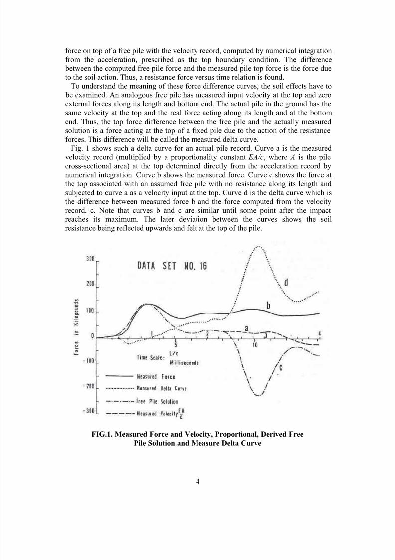
force on top of a free pile with the velocity record, computed by numerical integrationfrom the acceleration, prescribed as the top boundary condition. The difference between the computed free pile force and the measured pile top force is the force dueto the soil action. Thus, a resistance force versus time relation is found.

To understand the meaning of these force difference curves, the soil effects have to

be examined. An analogous free pile has measured input velocity at the top and zeroexternal forces along its length and bottom end. The actual pile in the ground has thesame velocity at the top and the real force acting along its length and at the bottomend. Thus, the top force difference between the free pile and the actually measuredsolution is a force acting at the top of a fixed pile due to the action of the resistanceforces. This difference will be called the measured delta curve.

Fig. 1 shows such a delta curve for an actual pile record. Curve a is the measuredvelocity record (multiplied by a proportionality constant EA/c, where A is the pilecross-sectional area) at the top determined directly from the acceleration record bynumerical integration. Curve b shows the measured force. Curve c shows the force atthe top associated with an assumed free pile with no resistance along its length and

subjected to curve a as a velocity input at the top. Curve d is the delta curve which isthe difference between measured force b and the force computed from the velocityrecord, c. Note that curves b and c are similar until some point after the impactreaches its maximum. The later deviation between the curves shows the soilresistance being reflected upwards and felt at the top of the pile.

FIG.1. Measured Force and Velocity, Proportional, Derived Free

Pile Solution and Measure Delta Curve



5

In order to interpret the measured delta curve correctly, it is necessary to adopt asoil model which links pile displacements and velocities to soil resistance forces. Theshear strength versus deformation behavior can be represented as a firstapproximation by a straight line until at a certain deflection-called quake in the piledynamics literature-the ultimate shear resistance is reached. Thereafter the soil

strength usually increases at a rate smaller than in the beginning of the curve and can be neglected in dealing with relatively small dynamic displacements. For increasingdisplacements greater than the quake the stiffness then is assumed to be zero. Thevalue of the quake has been found not to be critical for pile driving analysis (2). Inanalyzing actual pile records, it is always assumed that a final set was obtained under the individual hammer blow considered. This condition places an upper bound on thequake values, as the quake must be smaller than the maximum displacementoccurring at all points along the pile. It was found that the displacement reached at thetime of maximum velocity can be a good estimate (3) for the quake. Using this valuereduces the number of unknowns in the soil model, as the value of the ultimate shear strength now describes the shear versus displacement behavior completely.

Using the model of a linear damper, dynamic resistance forces will be assumed to be proportional to pile velocities. As in the case of a shear resistance force, a damper will induce waves which travel in both directions along the pile. The stress waves dueto dampers continually change magnitude to reflect the rapid changes in velocityduring impact driving.

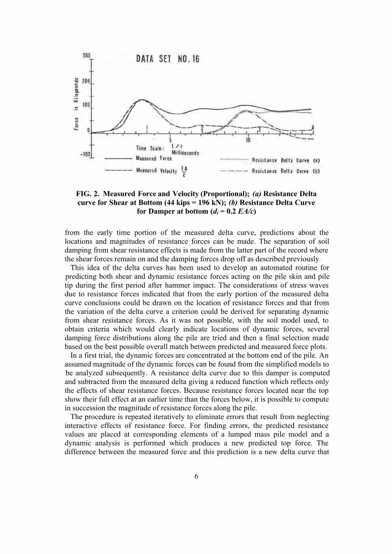
The action of a resistance force at some particular point along the pile or at the piletip can be represented by a resistance delta curve. This is defined as the force inducedon a fixed pile top while the bottom end is free and only the resistance force under investigation acts along the pile. It includes both the effect of the resistance wavemoving upwards and the resistance wave moving downwards and subsequentlyreflected from the pile tip. In the case of a shear force, the resistance delta curvereaches a level value because of the assumed elastoplastic sail resistance model.Consequently, the shear resistance is seen at the top as a constant value until theeffect of stress reversal is felt, making it possible to compute both its magnitude andlocation along the pile. The magnitude of resistance is determined from the force feltat the top and the location of resistance from the time after impact required for thewave to reach the top. For the case of a shear resistance force acting at the pile tip, theresistance delta curve is shown in Fig. 2. It can be observed that at time 2 L/c (the timerequired for the stress wave to travel the length of the pile and return) after themaximum velocity due to the reflections, the value of the resistance delta curve becomes twice the ultimate shear resistance force (in this case 2 x 44.0 kips = 2 x 196kN). Fig. 2 shows a resistance delta curve for a damper at the toe. Note that the shear resistance effect maintains a constant value while the damper resistance effect dropsoff quickly due to the decrease in the velocity. This important difference permits thetwo types of soil resistance forces to be distinguished.

The measured delta curve considered previously represents the superposition of resistance delta curves for all soil forces acting at various locations along the pile.Because each soil resistance force takes a longer time to reach the top at increasinglylower depths along the pile, each level of resistance can be isolated separately. Thus,



6

from the early time portion of the measured delta curve, predictions about thelocations and magnitudes of resistance forces can be made. The separation of soildamping from shear resistance effects is made from the latter part of the record wherethe shear forces remain on and the damping forces drop off as described previously.

This idea of the delta curves has been used to develop an automated routine for predicting both shear and dynamic resistance forces acting on the pile skin and piletip during the first period after hammer impact. The considerations of stress waves

due to resistance forces indicated that from the early portion of the measured deltacurve conclusions could be drawn on the location of resistance forces and that fromthe variation of the delta curve a criterion could be derived for separating dynamicfrom shear resistance forces. As it was not possible, with the soil model used, toobtain criteria which would clearly indicate locations of dynamic forces, severaldamping force distributions along the pile are tried and then a final selection made based on the best possible overall match between predicted and measured force plots.

In a first trial, the dynamic forces are concentrated at the bottom end of the pile. Anassumed magnitude of the dynamic forces can be found from the simplified models to be analyzed subsequently. A resistance delta curve due to this damper is computedand subtracted from the measured delta giving a reduced function which reflects only

the effects of shear resistance forces. Because resistance forces located near the topshow their full effect at an earlier time than the forces below, it is possible to computein succession the magnitude of resistance forces along the pile.

The procedure is repeated iteratively to eliminate errors that result from neglectinginteractive effects of resistance force. For finding errors, the predicted resistancevalues are placed at corresponding elements of a lumped mass pile model and adynamic analysis is performed which produces a new predicted top force. Thedifference between the measured force and this prediction is a new delta curve that

FIG. 2. Measured Force and Velocity (Proportional); (a) Resistance Deltacurve for Shear at Bottom (44 kips = 196 kN); (b) Resistance Delta Curve

for Damper at bottom (d i = 0.2 EA/c)



7

indicates the errors in the predicted resistance force distribution and provides a basisfor determining corrections. The process is repeated until the match cannot be further improved. Resulting matches between measured and predicted force records will beillustrated.

Other analyses are also used, with the dynamic forces uniformly distribution along

the pile or apportioned between skin and toe, with little change in predicted capacity but differences in top force matches. Subsequently, a final prediction is computed byminimizing a least square integral of the final delta curves. This can be accomplished by linear combination of the three individual sets of results and leads to a dampingand shear resistance distribution with the best possible match.

The preceding method of dynamically analyzing a pile using measured in-putquantities has limitations which should be mentioned. First, and most important, itwas found from acceleration and force records taken at the pile bottom (3) that thesoil model only approximates the soil behavior. Cohesive soils showed a lesssatisfactory agreement than cohesionless soils. Second, the method requires that thehammer impact produces a stress wave with a short rise time. If, as an extreme

example, the loading were of a static nature, then no distinction between locations of resistance forces were possible. Finally, it is not possible to predict the distribution of damping and static resistance forces independently. For this reason the method wasdesigned to optimize the match between measured and computed pile top force. Thisapproach might fail where large damping is encountered because of the limitations of the soil model. To introduce another soil model could improve the method. Work iscurrently being done in this area.

SIMPLIFIED METHODS

These methods also use the force and acceleration records and have beenincorporated by the Ohio Department of Highways for use in special purpose fieldcomputers for construction control during driving (4, 5). The first method, denoted asPhase 1, is based on a rigid body pile model and, in order to eliminate dampingeffects, on equilibrium at the instant when the pile velocity is zero. In this case thestatic resistance R 0 is given by

R0 = F(t 0 ) - Ma(t 0 ) (1)

in which t 0 = the time of zero velocity at the pile top; M = pile mass; F(t 0) the topforce at time t 0; and a(t 0) = the top acceleration at time t 0.

Because of the oscillations of the force and acceleration records in theneighborhood of t 0, due primarily to pile-hammer interaction, the results of Phase Ihave exhibited considerable scatter. To improve the predictions, a Phase 11 methodwas proposed (6) which eliminated the oscillation effect of the acceleration by takingaverage values. This gives the static bearing capacity as

∫ −−=

1

2

t

t 21

00 dt )t ( at t

M )t ( F R (2)



8

Usually t 1, is taken as the time of maximum force and t 2 is set equal to t 0 the time of zero velocity.

The Phase II method has been improved upon recently by use of the dynamictraveling wave analysis and leads to the following result denoted as Phase IIa (3):

∫ +

−

++

= )c / L2( t

t

11

0

1

1

dt )t ( a

c

L2

M

2

c L2t F )t ( F

R (3)

In other words, the best averaging scheme from a theoretical point of view is thatwhich takes averages over a time equal to the period of oscillation, 2 L/c. To eliminateas much as possible the dynamic viscous effects, t 1 is set equal to t 0, in Eq. 3. Amodification of this choice of t 1 must be employed in cases where the velocity reachesno zero value within the analyzed record (Piles with low capacity reach zero velocityoften only a long time after impact). Such modifications are reported in Ref. 3. The

comparison of the simplified Phases I, II and IIa with the more exact traveling wavesolution is presented and analyzed in the following.

CORRELATION PROCEDURE

Experimental data were obtained from both specially instrumented and constructionload test piles. Complete sets of data were available for analysis from 24 tests. Adescription of the piles is given in Table 1.

Several results can be predicted from a single data set when applying the methodsreviewed previously. These predictions are summarized as follows: (1) Static bearingcapacity; (2) shear resistance distribution along the pile; and (3) pile top force during

static loading versus pile penetration.The latter item is predicted by using the shear resistance forces along the pile in a

static load-displacement analysis and the assumed elastoplastic soil model. Such ananalysis produces a pile top force versus displacement relation which can becompared with the same curve from the actual field load test.

Load versus deflection curves obtained in a static load test often show increasingstrength values with pile top deflections much larger than those which are reachedunder a hammer blow. Thus, the prediction of static bearing capacity from dynamicmeasurements must be related to displacements of the pile actually experienced under the blow. A question arises, therefore, as to the value with which to compare the predicted bearing capacity.

Using data set No. 3 as an example, this question will now be examined. Waveanalysis was applied to this data set and both damping and shear resistance forceswere predicted. The predicted shear resistance distribution was then used for a staticanalysis. The load versus penetration (LP) curve resulting from this analysis and thecorresponding curve measured in the field static load test are both plotted in Fig. 3(b).Both LP curves show similar behavior up to a point where the predicted load curvereaches its ultimate capacity. The measured LP curve, however, shows further strength increase without an indication that an ultimate bearing capacity is reached.



9

T A B L E 1 . -

D e s c r i p t i o n o f T e s t P i l e s

D a t e

D a t a s e t

n u m b e r

( 1 )

P i l e n a m e

( 2 )

D r i v e n

( 3 )

S t a t i c a l l y

T e s t e d

( 4 )

D y n a m i c a l l

y t e s t e d

( 5 )

L e n g t h , L , ( B e l o w

A c c e l e r o m e

t e r ) i n

f e e t ( 6 )

A r e a , A , i n

s q u a r e i n c h e s

( 7 )

H a m m e r

( 8 )

1

C - 1

1 2 - 2 8 / 6 6

1 2 - 3 0 - 6 6

1 - 3 - 6 7

5 8

5 . 8 1

D - 1 2 a

2

5 3 1 - 7 0

4 - 1 2 - 6 7

5 - 1 2 - 6 7

4 - 1 3 - 6 7

7 0

5 . 8 1

D - 1 2

3

5 3 1 - 7 6

4 - 1 3 - 6 7

4 - 1 7 - 6 7

4 - 1 8 - 6 7

8 2

5 . 8 1

D - 1 2

4

5 3 1 - 8 3

4 - 1 8 - 6 7

4 - 1 8 - 6 7

5 - 1 8 - 6 7

8 2

5 . 8 1

D - 1 2

5

F - 3 0

6 - 2 1 - 6 7

6 - 2 1 - 6 7

6 - 2 1 - 6 7

3 2 . 5

9 . 8 2

L B b

6

F - 3 0 A

6 - 2 1 - 6 - 6 7

6 - 2 8 - 6 7

6 - 2 8 - 6 7

3 2 . 5

9 . 8 2

L B

7

F - 5 0

6 - 2 8 - 6 7

6 - 2 8 - 6 7

6 - 2 8 - 6 7

5 0 . 5

9 . 8 2

L B

8

F - 5 0 A

6 - 2 8 - 6 7

7 - 5 - 6 7

7 - 6 - 6 7

5 0 . 5

9 . 8 2

L B

9

F 6 0

7 - 7 - 6 7

7 - 7 - 6 7

7 - 7 - 6 7

5 9 . 5

9 . 8 2

L B

1 0

F - 6 0 A

7 - 7 - 6 7

7 - 2 0 - 6 7

7 - 2 0 - 6 7

5 9 . 5

9 . 8 2

L B

1 1

C i n c i n n a t i

1 2 - 2 2 - 6 7

1 - 4 - 6 8

1 - 4 - 6 8

6 9

6 . 6 6

D - 1 2

1 2

2 7 2 T o l e d o

4 - 1 0 - 6 8

4 - 1 7 - 6 8

5 - 1 8 - 6 8

5 4

6 . 6 6

L B

1 3

T o - 5 0

9 - 6 - 6 8

9 - 6 - 6 8

9 - 6 - 6 8

4 9

9 . 8 2

D - 1 2

1 4

T o - 5 0 A

9 - 6 - 6 8

9 - 9 - 6 8

9 - 1 0 - 6 8

4 9

9 . 8 2

D - 1 2

1 5

T o - 6 0

9 - 1 1 - 6 8

9 - 1 1 - 6 8

9 - 1 1 - 6 8

5 9

9 . 8 2

D - 1 2

1 6

T o - 6 0 A

9 - 1 1 - 6 8

9 - 1 8 - 6 8

9 - 1 8 - 6 8

5 9

9 . 8 2

D - 1 2

1 7

L o g a n

1 1 - 2 5 - 6 8

1 1 - 5 - 6 8

1 1 - 5 - 6 8

5 7

6 . 6 6

D - 1 2

1 8

W - 5 6

6 - 1 1 - 6 9

6 - 1 8 - 6 9

6 - 1 8 - 6 9

5 5

6 . 6 6

D - 1 2

1 9

W - 7 6

6 - 1 9 - 6 9

6 - 2 4 - 6 9

6 - 2 4 - 6 9

7 6

6 . 6 6

D - 1 2

2 0

C h i l l i c o t h e

6 - 1 8 - 6 9

6 - 2 5 - 6 9

9 - 2 5 - 6 9

4 0 . 5

6 . 6 6

D - 1 2

2 1

R i - 5 0

1 - 6 - 7 0

1 - 6 - 7 0

1 - 6 - 7 0

4 9

9 . 3 1

D - 1 2

2 2

R i - 5 0

1 - 6 - 7 0

1 - 6 - 7 0

1 - 6 - 7 0

4 9

9 . 3 1

D - 1 2

2 3

R i - 6 0

1 - 9 - 1 7 0

1 - 9 - 7 0

1 - 9 - 7 0

6 1 . 5

9 . 3 1

D - 1 2

A l l p i l e s w e r e o f 1

2 - i n . d i a m p i p e

a D - 1 2 = D e l m a g

1 f t = 0 . 3 0 5 m . ; 1 i n . = 2 . 5 4 c m

b L B = L i n k b e l t 4 4 0 .



10

In a static test, a load is applied on top of the pile which compresses both the pile

and the soil. The elastic pile deformations were relatively large for the pilesencountered in this study. (The pile of the data set No. 3, for example, compresses0.52 in. = 1.32 cm under a uniform load of 100 kips = 445 kN). Because of pileelastic deformations, the pile tip moves less than the pile top and during a static load

FIG. 3. Data Set No. 3: (a) Comparison between Measured and Predicted

Pile Top Force and Measured Pile Top Velocity;(b)

Comparison betweenMeasured and Predicted Static Load Versus Penetration Curve



11

test the pile tip will usually be the last point along the pile to reach the quake penetration. If the assumed static elastoplastic soil resistance law were valid, then theultimate capacity would be reached at that pile top penetration occurring when the tipreaches the quake displacement. This is the case only for the assumed soil model; butin reality, the soil resistance forces frequently increase even after the quake

penetration is exceeded, although at a smaller rate. Then a higher dynamic penetration will produce a higher shear resistance. Because the pile penetrationsduring driving are usually small, the assumed elastoplastic relationship stillestablishes a good approximation for the dynamic case. However, the static load testwill not reach, at various points along the pile, the same penetration valuessimultaneously as the dynamic load and comparison between the dynamic predictionand static load test cannot be exact. In order to find a reasonable comparison betweenthe static load test result and the dynamic prediction, the following correlationscheme is, therefore, proposed: From the dynamic analysis compute the maximumdeflection of the pile top under the hammer blow and obtain the corresponding loadvalue from the LP curve of the field static load test. Call load Rd the bearing capacity

at maximum dynamic deflection. The predicted capacity from dynamic measurements R0 will then be compared with Rd . For most cases, the static load penetration curvehas leveled off at the maximum dynamic deflection, and differences with other definitions of bearing capacity (yield, ultimate) are small.

RESULTS

In this section, the results of applying wave analysis and simplified predictions toall data sets listed in Table 1 are reviewed and compared with results of the static loadtest. Exceptions were data sets Nos. 1, 2, 4, and 12, in which the wave analysis couldnot be applied because the rise time of force and velocity was longer than 2L/c, sothat reflection waves returned from the pile bottom before the maximum velocity wasreached at the pile top. The reason for such records is probably an early combustionin the hammer which cushioned the blow excessively.

Simplified Methods - The results from three simplified methods introduced previously are listed in Cols. 5, 6 and 7 of Table 2. Usually more than one blow had been analyzed. The average value was listed in Table 2.

Comparing the simplified predictions with the pile capacity at maximum dynamicdeflection Rd in Col. 3, it can be seen that Phase IIa usually gave the better agreement. Some of the individual piles will be subsequently analyzed in connectionwith wave analysis results.

Wave Analysis - As an example, consider pile 531-76 (data set No. 3) having arecord with the usual impact properties. Fig. 3(a) shows a plot of the top forces both predicted by wave analysis and measured. Also, the velocity measured at the pile top(used as input for the analysis) is plotted after being multiplied by EA/c. Agreement between predicted and measured pile top force is good throughout the time intervalconsidered. Fig. 3(b) represents the LP curves both measured and predicted. Theforce at the point where the maximum dynamic deflection, shown by the dotted line,intersects the measured LP curve is Rd . Thus, correlation between Rd and R0 theultimate bearing capacity predicted, is good (see also Table 2). Fig. 4 shows both a



1 2

T A B L E 2 . S u m m a r y

o f R e s u l t s f o r P r e d i c t i o n S t a t i c B e a r i n g C a p a c i t y u s i n g S i m p l i f i e

d M e t h o d s a n d W a v e A n a l y s i s

L o a d T e s t R e s u l t s a

P r e d i c t i o n s b

D a t a s e t

n u m b e r

( 1 )

P i l e n a

m e

( 2 )

A t m a x i m u m

d y n a m i c

d e f l e c t i o n , R d

( 3 )

A t u l t i m a t e

R u

( 4 )

P h a s e I , R 0

( 5 )

P h a s e I I , R 0

( 6 )

P h a

s e I I a ,

R 0

( 7 )

W a v e d

a n a l y s i s R 0

( 8 )

W a v e e

a n a l y s i s , R 0

( 9 )

T o t a l e

d a m p i n g

f o r c e s , m a x

D

( 1 0 )

1

C - 1

1 8 0

1 9 2

1 7 4 1

1 3 8 1

1

7 6 3

c

c

c

2

5 3 1 - 7 0

1 2 2

1 9 0

2 0 1 3

1 9 7 3

1

4 1 3

c

c

c

3

5 3 1 - 7 6

1 5 1

1 9 8

1 7 0 4

1 5 7 4

1

1 5 4

1 5 9 1

1 5 9

1 5

4

5 3 1 - 8 3

1 1 0

2 0 0

2 1 1 3

1 8 7 3

1

4 3 3

c

c

c

5

F - 3 0

9 7

1 0 3

1 2 5 5

1 1 3 5

1

1 0 5

8 8

8 8

3 9

6

F - 3 0 A

1 0 7

1 1 4

1 6 2 4

1 5 2 4

1

6 4 5

1 3 6

1 3 6

2 4

7

F - 5 0

1 7 2

2 2 4

2 8 1 3

1 9 7 3

1

7 7 3

1 6 7

1 6 7

4 1

8

F - 5 0 A

2 0 0

2 3 8

2 9 4 4

2 5 8 4

2

0 5 4

2 3 0

2 3 0

5 2

9

F - 6 0

1 7 6

2 0 4

2 8 8 4

2 5 1 4

2

0 7 4

2 0 0

2 0 0

2 5

1 0

F - 6 0 A

1 7 4

2 4 2

2 5 5 3

2 2 6 3

1

8 8 3

1 9 8

1 9 8

5 2

1 1

C i n c i n n a t i

1 3 7

1 9 0

2 5 0 3

1 8 5 3

1

3 8 3

1 2

2 7 2

1 8 3

2 2 1

3 1 5 7

2 7 5 7

2

6 7 7

c

c

c

1 3

T o - 5 0

6 0

6 9

6 9 3

6 3 3

7 7 5

6 2

6 2

5 7

1 4

T o - 5 0

A

9 3

9 4

1 2 1 8

1 2 9 8

1

0 5 8

1 1 9

1 1 9

8 8

1 5

T o - 6 0

3 2

4 3

8 9 4

8 1 4

7 7 4

5 5

5 5

6 9

1 6

T o - 6 0

A

7 5

8 6

1 4 1 3

1 3 7 3

1

1 3 3

1 1 9

1 1 9

1 0 6

1 7

L o g a n

1 6 5

2 2 0

2 7 5 4

2 2 3 4

1

8 0 4

1 8

W - 5 6

9 0

9 2

2 0 7 4

2 2 7 4

1

6 1 4

1 9

W - 7 6

1 2 5

1 6 0

2 7 6 5

2 6 4 5

1

6 7 3

2 0

C h i l i c

o t h e

1 5 2

2 0 7

3 1 6 3

2 0 0 3

1

8 0 3

2 1

R i - 5 0

4 0

4 6

g

g

6 4 3

4 5

4 5

8 8

2 2

R i - 5 0 A

6 4

6 4

g

g

1

2 0 3

8 5

8 5

1 0 5

2 3

R i - 6 0

1 7 6

f

2 6 4 3

2 5 1 3

1

4 0 3

1 8 9

1 8 9

9 2

2 4

R i - 6 0 A

1 7 4

f

1 7 9 2

1 8 4 2

1

6 2 3

1 9 4

1 9 4

4 8

a A l l r e s u l t s i n k i p s ( 1 k i p = 4 . 4 5 k N )

b S u p e r s c r i p t s o n p r e d i c t i o

n s i n d i c a t e t h e n u m b e r o f b l o w s a n a l y z e d a n d a v e r a g e d .

c N o t a n a l y z e d b y w a v e m e t h o d b e c a u s e o f w e a k i m p a c t .

d A n a l y s i s r e s u l t s f r o m m o

r e t h a n o n e b l o w .

e A n a l y s i s r e s u l t s f r o m

o n e b l o w c o r r e s p o n d i n g t o F i g s . 3 t h r o u g h 6 .

f L o a d t e s t i n c o m p l e t e .

g N o z e r o v e l o c i t y w a s

r e a c h e d w i t h i n r e c o r d a n a l y z e d .



13

soil description and the predicted resistance force distribution in the pile (atmaximum dynamic deflection).

The predicted shear resistance forces are acting at the lower pile half and aredistributed rather uniformly. Because this pile was an actual construction pile, noforce measurements were obtained from locations below grade. However, the blowcount (number of blows per unit pile penetration) gradually increased with depth,thus providing some correlation with the prediction of resistance distribution.

FIG. 4. Soil Description and Predicted Force Distribution I Pile at

Predicted Ultimate Capacity



14

Dynamic resistance forces predicted were small and concentrated at the pile tip. Themagnitude of the sum of the maxima of all dynamic forces is listed in Table 2, Col.10.

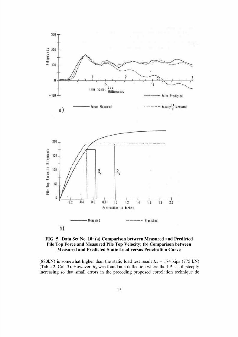
Fig. 5(a) shows the match of measured and predicted pile top force for data set No.10. The pile was a special test pile with additional strain gages at the pile tip andclose to the pile center. The data were obtained after a setup period of 1 week after driving. The predicted bearing capacity R0 (listed in Table 2, Col. 9), of 198 kips

FIG. 4 Continued



15

(880kN) is somewhat higher than the static load test result Rd = 174 kips (775 kN)(Table 2, Col. 3). However, Rd was found at a deflection where the LP is still steeplyincreasing so that small errors in the preceding proposed correlation technique do


Pile Top Force and Measured Pile Top Velocity; (b) Comparison between

Measured and Predicted Static Load versus Penetration Curve



16

affect the agreement. Better agreement with measured results is usually obtained byanalyzing several blows, as indicated in Table 2. Both measurements and predictions(see Fig. 4) indicate that most of the static resistance results from point bearing. Themaximum dynamic resistance (all damping was predicted to act concentrated at the pile top) was approximately 25% of the total static bearing capacity (see Table 2).

The results for another special instrumented test pile (data set No. 16) aresummarized in Figs. 5 and 6. The soil was highly cohesive, which explains why themaximum damping force predictions are approximately equal to the sum of the shear resistance forces (Table 2). Although the prediction of static bearing capacity was toohigh (119 kips versus 75, i.e., 530 kN versus 333), a clear indication of theimportance of skin friction forces on the pile was found.

Data sets Nos. 5 through 10 were obtained at the same pile but for different lengthsand both before and after a setup period. Data sets Nos. 5 and 6 were obtained whenthe pile was only 33.5 ft (10.2 m) long. During the static load test strainmeasurements were taken at both the top and the pile toe. The match between the predicted and measured pile top forces was poor at time 2L/c after maximum velocity

and later. Agreement is good between R0 from wave analysis and Rd for data set No. 5and fair for data set No. 6. A deficiency of the predictions can be found in thedistribution of shear resistance forces (Fig. 4). Apparently, the wave method failed to predict the proper pile tip resistance force. However, a shift of the predictions over one analysis element (10 elements were always used for the computations presented)is equivalent to a time shift of only 0.2 msec (the time necessary for the wave totravel 1/10 of the pile length). The accuracy of both the measurements and themethod seems not to be sufficient to distinguish forces acting over such smalldistances.

Data set No. 7 was obtained after extending the aforementioned 33.5-ft (10.2-m)long pile by an additional section of 18 ft (5.5 in). Strain records were taken at threelocations along the pile during the static load tests. The shear resistance distributionshows more pile tip resistance in the prediction than in the measurements. However,the fact that the pile had basically point bearing properties is brought out in bothmeasurement and prediction. The results from analyzing data set No. 9 were verysimilar to those for set No. 10, which have already been considered.

Piles To-50 and To-60 were two special test piles of 50-ft and 60-ft (15.3-m and18.3-m) length equipped with strain gages for force measurements below grade. Dataset No. 13 was obtained immediately after driving pile To-50 and data set No. 14after a setup period of 3 days. The soil was a silty clay. A low ultimate capacity of 69kips (307 kN) was found in the load test immediately after driving. The predictionsare good as shown in Fig. 4 and in Table 2.

Data set No. 14 yielded a bearing capacity which was too high. From forcemeasurements along the pile taken during the load test it was found that relativelylarge resistance forces were acting along the skin of the pile. Apparently, these skinforces were predicted for locations lower than found in the static load test probablythe uncertainty about damping distribution, mentioned above, lead to this result. Themagnitude of the pile toe force, however, was predicted correctly.



17

Data sets Nos. 15 and 16 were obtained from the second special test pile at the same

site as the pile just reviewed. The pile was longer; however, its ultimate bearingcapacity was smaller than for the shorter pile. Very similar observations as in Nos. 13


Pile Top Force and Measured Pile Top Velocity; (b) Comparison between

Measured and Predicted Static Load Versus Penetration Curve



18

and 14 can be made on the results of both data sets. (Table 2 and Fig. 4). Data set No.16 was previously considered.

Finally, results from another special test pile are presented. The pile was driven andtested in two steps. First the pile, Ri-50, was driven to a depth of 48 ft (14.6 m). This pile was embedded in silty and clayey soil (Fig. 4). Later the pile was driven until a

stiff soil layer was reached and driving became very hard (Ri-60). The two data sets(Nos. 21 and 22) for the shorter pile gave results similar to the test piles To-50 andTo-60 (data sets Nos. 13 through 16). The difference was that the waiting period didnot influence the soil properties as much as in the case of the To-piles. Again, as inother cases of piles in cohesive soils, relatively high dynamic and skin resistanceforces were observed. It should be mentioned that measurements and analysiscorrectly reflected the strength gain of shear forces along the pile skin during thewaiting period. This can be seen by comparing the force distributions along the pilefor data sets Nos. 21 and 22 in Fig. 4.

Other results from construction piles are also listed in Table 2. In these cases nomeasurements had been taken along the pile, so that resistance distributions cannot be

compared. In general, it was found that piles in granular, materials (Nos. 11, 17 and20) showed a point bearing distribution while the, two W piles (Nos. 18 and 19) wereof the skin friction type. These two piles were driven in soils with plasticity indexesin the neighborhood of 15.

It should be mentioned that the prediction of ultimate capacity (Table 2, Col. 6) was poorest for pile W-56, probably because of the cohesiveness of the soil. The poorestcorrelation between dynamic predictions and static tests on a percentage basisoccurred for piles having a very small capacity. Actually, such piles are not typical of practice and a percentage comparison is perhaps inappropriate.

STATISTICAL INVESTIGATION ON BEARING CAPACITY

PREDICTIONS

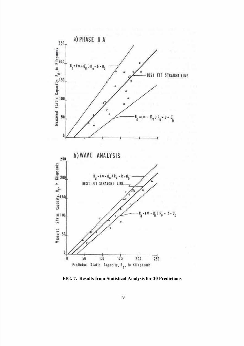
A brief statistical investigation of the Phase IIa and wave analysis results was performed. Twenty sets of predictions are available including all data sets which wereanalyzed by the automated prediction routine. The variety of soil conditionsrepresented is a fairly representative statistical sample. The computations are done assuggested by Olson and Flaate (8) for the treatment of results from the energyformulas. Accordingly, the, measured capacity, Rd , is thought of as being a functionof the predicted capacity, R0. A best fit straight line

Rd = m R0 + b (4)

is then determined for the prediction scheme by the least square method, The resultsare shown in Figs. 7(a) and 7(b) for the Phase IIa and the wave analysis, respectively.As a measure of the variability in the predictions the variances,

2

mσ and 2

bσ of m and b, are also calculated. For illustrations, the lines

Rd = (m ± σ m ) R0 + (b ± σ b ) (5)



19

FIG. 7. Results from Statistical Analysis for 20 Predictions



20

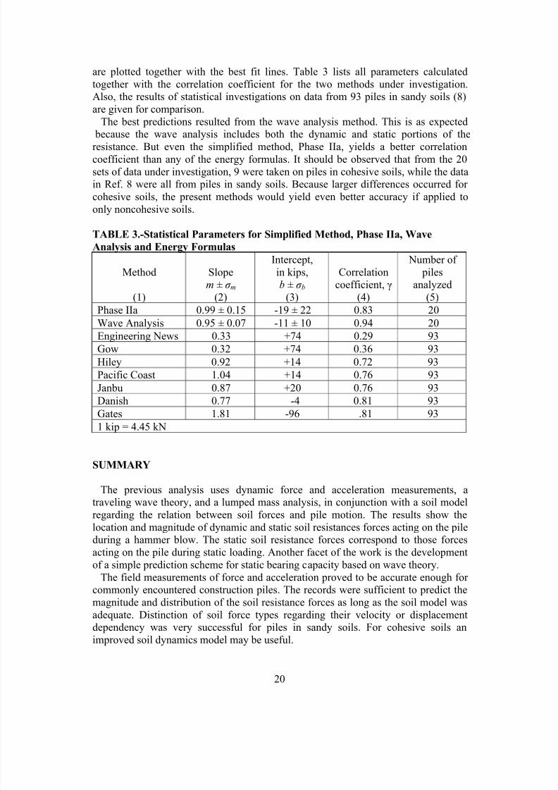
are plotted together with the best fit lines. Table 3 lists all parameters calculatedtogether with the correlation coefficient for the two methods under investigation.Also, the results of statistical investigations on data from 93 piles in sandy soils (8)are given for comparison.

The best predictions resulted from the wave analysis method. This is as expected

because the wave analysis includes both the dynamic and static portions of theresistance. But even the simplified method, Phase IIa, yields a better correlationcoefficient than any of the energy formulas. It should be observed that from the 20sets of data under investigation, 9 were taken on piles in cohesive soils, while the datain Ref. 8 were all from piles in sandy soils. Because larger differences occurred for cohesive soils, the present methods would yield even better accuracy if applied toonly noncohesive soils.

TABLE 3.-Statistical Parameters for Simplified Method, Phase IIa, Wave

Analysis and Energy Formulas

Method

(1)

Slopem ± σ m(2)

Intercept,

in kips,b ± σ b(3)

Correlationcoefficient, γ (4)

Number of

pilesanalyzed(5)

Phase IIa 0.99 ± 0.15 -19 ± 22 0.83 20

Wave Analysis 0.95 ± 0.07 -11 ± 10 0.94 20

Engineering News 0.33 +74 0.29 93

Gow 0.32 +74 0.36 93 Hiley 0.92 +14 0.72 93 Pacific Coast 1.04 +14 0.76 93 Janbu 0.87 +20 0.76 93 Danish 0.77 -4 0.81 93 Gates 1.81 -96 .81 93 1 kip = 4.45 kN

SUMMARY

The previous analysis uses dynamic force and acceleration measurements, atraveling wave theory, and a lumped mass analysis, in conjunction with a soil modelregarding the relation between soil forces and pile motion. The results show thelocation and magnitude of dynamic and static soil resistances forces acting on the pileduring a hammer blow. The static soil resistance forces correspond to those forces

acting on the pile during static loading. Another facet of the work is the developmentof a simple prediction scheme for static bearing capacity based on wave theory.

The field measurements of force and acceleration proved to be accurate enough for commonly encountered construction piles. The records were sufficient to predict themagnitude and distribution of the soil resistance forces as long as the soil model wasadequate. Distinction of soil force types regarding their velocity or displacementdependency was very successful for piles in sandy soils. For cohesive soils animproved soil dynamics model may be useful.



21

The present method bypasses a major shortcoming of pile dynamic analyses foundin the literature, namely the uncertainty of hammer input and soil parameters. In fact,the prediction scheme can be used to give information on soil behavior. This is incontrast to the usual procedures of first obtaining the soil properties by laboratorytesting and then performing the pile analysis. Also information from the analysis may

be obtained which would indicate characteristics of hammer types that would be mostefficient for driving in particular soils. This is being studied further.The predictions of static bearing capacity show a better correlation than those

obtained from existing methods (8, 11). Another important result of the studies presented herein was the improvement of an existing simplified prediction scheme for static bearing capacity. As a further step to a realistic dynamic pile testing procedure,the Phase IIa prediction scheme was incorporated in a special purpose computer which is currently being tested on actual construction piles. Additional tests on pileswith materials such as timber and concrete, piles of greater length and of variablecross section will be performed to further check the proposed methods.

It is expected that the proposed method will reduce foundation costs. First, static

load tests will be less frequently necessary. Probably more important will be the useof these analyses and predictions to reduce the rather large margins between indicated bearing and capacity required by design. The economic use of multiple dynamic test piles, perhaps in conjunction with a single static test pile, will further add to thereliability of test results. Certainly the correlation between dynamic prediction andstatic measurement on the large number of piles tested cannot be ignored.

ACKNOWLEDGMENTS

The work reported herein was sponsored by the Ohio Department of Highways andthe Bureau of Public Roads. The writers would like to express their appreciation to C.R. Hanes, R. M. Dowalter and R. A. Grover, all of the Ohio Department of Highwaysfor their advice and assistance. The opinions, findings and conclusions expressed inthis publication are those of the writers and not necessarily those of the State or theBureau of Public Roads.

APPENDIX I.-REFERENCES

1. Donnell, L. B., "Longitudinal Wave Transmission and Impact," Journal of Applied Mechanics. Transactions, ASME, APM-52-14, 1930.

2. Forehand, P. W., and Reese, J. L., "Predictions of Pile Capacity by the WaveEquation," Journal of the Soil Mechanics and Foundations Division, ASCE,Vol. 90, No. SM2, Proc. Paper 3820, March, 1964, pp. 1-25.

3. Goble, G. G., Rausche, F., and Moses, F., "Dynamic Studies on the BearingCapacity of Piles - Phase III," Final Report to the Ohio Department of

Highways, Case Western Reserve Univ., Cleveland, Ohio, Aug., 1970.4. Goble, G. G., and Rausche, F., "Pile Load Test by Impact Driving," Highway),

Research Record No. 333, Pile Foundations, Highway Research Board,Washington, D.C., 1970.



22

5. Goble, G. G., Scanlan, R, H., and Tomko, J. J., "Dynamic Studies on theBearing Capacity of Piles," Highway Research Record No. 167, Bridges and

Structures, Highway Research Board, Washington, D.C., 1967.6. Goble, G. G., et al., "Dynamic Studies on the Bearing Capacity of Piles-Phase

II," Final Report to the Ohio Department of Highways, Case Western Reserve

Univ., Cleveland, Ohio, July 1, 1968.7. Lowery, L. L., et al., "Pile Driving Analysis-State-of-the-Art," Research Report 33-13 (Final), Texas Transportation Institute, Texas A & M Univ., Jan. 1969

8. Olson, R. E., and Flaate, K. S., "Pile Driving Formulas for Friction Piles inSand," Journal of the Soil Mechanics and Foundations Division, ASCE, Vol.93, No. SM6. Proc. Paper 5604, Nov., 1967, pp. 279-296.

9. Rausche, F., "Soil Response from Dynamic Analysis and Measurements onPiles," thesis presented to the Case Western Reserve University, at Cleveland,Ohio, in 1970, in partial fulfillment of the requirements for the degree of Doctor of Philosophy.

10. Samson, C. H., Hirsch, T. L., and Lowery, L. L., "Computer Study of Dynamic

Behavior of Piling," Journal of the Structural Division. ASCE, Vol. 89, No.ST4, Proc. Paper 3608, Aug., 1963, pp. 413-450.11. Scanlan, R. H., and Tomko, J. J., "Dynamic Prediction of Pile Static Bearing

Capacity," Journal of the Soil Mechanics and Foundations Division, ASCE,Vol. 95, No. SM2, Proc. Paper 6468, Mar., 1969, pp. 583-604.

12. Smith, E. A. L., "Pile Driving Analysis by the Wave Equation," Journal of the

Soil Mechanics and Foundations Division, ASCE, Vol. 86, No. SM4, Proc.Paper 2574, Aug., 1960, pp. 35-61.

13. Timoshenko, S., and Goodier, J. M., McGraw-Hill Book Co., 2nd ed., 1951, p.438.

APPENDIX II.-NOTATION

The following symbols are used in this paper:

A = pile cross-sectional area;a(t) = pile top acceleration;

b = intercept of best fit straight line (Eq. 4);c = wave speed in pile;

E = Young's modulus of pile material; F(t) = pile top force;

L = pile length;M = pile mass;m = slope of best fit straight line;

max D = sum of maxima of all damping forces; Rd = measured static pile capacity at maximum dynamic deflection; R0 = predicted static pile capacity; Ru = measured ultimate static pile capacity;γ = correlation coefficient;t = time variable;



t 0 = time of zero velocity;t 1 , t 2 = fixed time values;

ρ = mass density of pile material;σ b = standard deviation of intercept (Eq. 5); andσm = standard deviation of slope (Eq. 5).

Soil Resistance Predictions From Pile Dynamics. Current Practices and Future Trends in Deep...

Documents

Transcript of Soil Resistance Predictions From Pile Dynamics. Current Practices and Future Trends in Deep...