SOIL MODELS AND VEHICLE SYSTEM DYNAMICS · soil models and vehicle system dynamics ulysses...

UNCLASSIFIED: Distribution Statement A. Approved for public release. #23850

SOIL MODELS AND VEHICLE SYSTEM DYNAMICS

Ulysses Contreras1

Guangbu Li2

Craig D. Foster3

Ahmed A. Shabana1

Paramsothy Jayakumar4

Michael D. Letherwood4

1 Department of Mechanical and Industrial Engineering, University of Illinois at Chicago, 842

West Taylor Street, Chicago, Illinois 60607 2

Department of Mechanical Engineering, Shanghai Normal University, 100 Guilin Road,

Shanghai, 200234 3

Department of Civil and Materials Engineering, University of Illinois at Chicago, 842 West

Taylor Street, Chicago, Illinois 60607 4

U.S. Army RDECOM-TARDEC, 6501 East 11 Mile Road, Warren, MI 48397-5000

Report Documentation Page Form ApprovedOMB No. 0704-0188

Public reporting burden for the collection of information is estimated to average 1 hour per response, including the time for reviewing instructions, searching existing data sources, gathering andmaintaining the data needed, and completing and reviewing the collection of information. Send comments regarding this burden estimate or any other aspect of this collection of information,including suggestions for reducing this burden, to Washington Headquarters Services, Directorate for Information Operations and Reports, 1215 Jefferson Davis Highway, Suite 1204, ArlingtonVA 22202-4302. Respondents should be aware that notwithstanding any other provision of law, no person shall be subject to a penalty for failing to comply with a collection of information if itdoes not display a currently valid OMB control number.

1. REPORT DATE 07 MAY 2013

2. REPORT TYPE Technical Report

3. DATES COVERED 12-06-2012 to 09-04-2013

4. TITLE AND SUBTITLE SOIL MODELS AND VEHICLE SYSTEM DYNAMICS

5a. CONTRACT NUMBER W56HZV-13-C-0032

5b. GRANT NUMBER

5c. PROGRAM ELEMENT NUMBER

6. AUTHOR(S) Ulysses Contreras; Guangbu Li; Ahmed Shabana; ParamsothyJayakumar; Michael Letherwood

5d. PROJECT NUMBER

5e. TASK NUMBER

5f. WORK UNIT NUMBER

7. PERFORMING ORGANIZATION NAME(S) AND ADDRESS(ES) Department of Mechanical and Industrial Engineering,University ofIllinois at Chicago,842 West Taylor Street,Chicago,IL,60607

8. PERFORMING ORGANIZATION REPORT NUMBER ; #23850

9. SPONSORING/MONITORING AGENCY NAME(S) AND ADDRESS(ES) U.S. Army TARDEC, 6501 East Eleven Mile Rd, Warren, Mi, 48397-5000

10. SPONSOR/MONITOR’S ACRONYM(S) TARDEC

11. SPONSOR/MONITOR’S REPORT NUMBER(S) #23850

12. DISTRIBUTION/AVAILABILITY STATEMENT Approved for public release; distribution unlimited

13. SUPPLEMENTARY NOTES

14. ABSTRACT The mechanical behavior of soils may be approximated using different models that depend on particularsoil characteristics and simplifying assumptions. For this reason, researchers have proposed andexpounded upon a large number of constitutive models and approaches that describe various aspects of soilbehavior. However, there are few material models capable of predicting the behavior of soils forengineering applications and are at the same time appropriate for implementation into finite element (FE)and multibody system (MBS) algorithms. This paper presents a survey of some of the commonly usedcontinuum-based soil models. The aim is to provide a summary of continuum-based soil models andexamine their suitability for integration with the large-displacement FE absolute nodal coordinateformulation (ANCF) and MBS algorithms. Special emphasis is placed on the formulation of soils used inconjunction with vehicle dynamics models. The implementation of these soil models in MBS algorithmsused in the analysis of complex vehicle systems is also discussed. Because semi-empirical terramechanicssoil models are currently the most widely used to study vehicle/soil interaction, a review of classicalterramechanics models is presented in order to be able to explain the modes of displacements that are notcaptured by these simpler models. Other methods such as the particle-based and mesh-free models are alsobriefly reviewed. A Cam-Clay soil model is used in this paper to explain how such continuum-mechanicsbased soil models can be implemented in FE/MBS algorithms.

15. SUBJECT TERMS Soil mechanics; Finite element; Multibody systems; Terramechanics.

16. SECURITY CLASSIFICATION OF: 17. LIMITATIONOF ABSTRACT

Public Release

18. NUMBEROF PAGES

94

19a. NAME OFRESPONSIBLE PERSON

a. REPORT unclassified

b. ABSTRACT unclassified

c. THIS PAGE unclassified

Standard Form 298 (Rev. 8-98) Prescribed by ANSI Std Z39-18

UNCLASSIFIED

Contreras et al. AMR-12-1012 2

ABSTRACT

The mechanical behavior of soils may be approximated using different models that depend on

particular soil characteristics and simplifying assumptions. For this reason, researchers have

proposed and expounded upon a large number of constitutive models and approaches that

describe various aspects of soil behavior. However, there are few material models capable of

predicting the behavior of soils for engineering applications and are at the same time appropriate

for implementation into finite element (FE) and multibody system (MBS) algorithms. This paper

presents a survey of some of the commonly used continuum-based soil models. The aim is to

provide a summary of continuum-based soil models and examine their suitability for integration

with the large-displacement FE absolute nodal coordinate formulation (ANCF) and MBS

algorithms. Special emphasis is placed on the formulation of soils used in conjunction with

vehicle dynamics models. The implementation of these soil models in MBS algorithms used in

the analysis of complex vehicle systems is also discussed. Because semi-empirical

terramechanics soil models are currently the most widely used to study vehicle/soil interaction, a

review of classical terramechanics models is presented in order to be able to explain the modes

of displacements that are not captured by these simpler models. Other methods such as the

particle-based and mesh-free models are also briefly reviewed. A Cam-Clay soil model is used in

this paper to explain how such continuum-mechanics based soil models can be implemented in

FE/MBS algorithms.

Keywords: Soil mechanics; Finite element; Multibody systems; Terramechanics.

UNCLASSIFIED


1. INTRODUCTION

There are a number of situations in which a vehicle may need to traverse an unprepared terrain. It

may happen that the only viable means of reaching a desired objective is through an off-road

route. In such an instance, it would be desirable to have an understanding of how a vehicles

design affects its performance in such an environment. Often, vehicles are specifically designed

for off-road usage. This is the case for military, construction, and agriculture vehicles as well as

unmanned/manned rovers. In all cases it is important to be able to predict (to varying degrees)

the conditions under which a vehicle may become incapacitated due to loss of traction. There are

other vehicle-terrain related effects that might need to be modeled. For instance, in the case of

agricultural vehicles, it is important to be able to predict the compaction induced in the soil. Soil

compaction has been determined to cause a reduction in crop yield. It is thus important to

minimize a vehicles impact on the terrain. Terramechanics is the field tasked with producing the

tools necessary to model the vehicle-terrain interaction over unprepared terrain.

Over the past decades, there have been a number of vehicle terrain interaction studies

published which explicitly treat the simplified vehicle dynamic equations of motion together

with the semi-empirical equations for the soil. One of the recent trends is the incorporation of

semi-empirical terramechanics equations or the co-simulation of finite element (FE) soil models

with MBS environments. These environments provide a framework in which the dynamic

interaction between vehicle and terrain may be modeled. Incorporation of FE soil within

multibody system algorithms can provide a higher fidelity simulation of the dynamic vehicle-

terrain interactions. The integration of these FE soil models with MBS algorithms for modeling

vehicle/soil interaction represents a challenging implementation and computational problem that

UNCLASSIFIED


has not been adequately covered in the literature. This integration is necessary in order to be able

to develop a more detailed and a more accurate vehicle/terrain dynamic interaction models.

The ability to capture the soil behavior modeled under dynamic loading conditions is of

particular interest in the FE/MBS approach to terramechanics. The mechanical characteristics of

soils, as with any other material, depend on the loading and soil conditions.

The mechanical characteristics of soils, as with any other material, depend on the loading

and material state. The response of the soil model to loading conditions depends on the

assumptions used in and the details captured by the specific model. Some approximations are

based on simple discrete elastic models that do not capture the distributed elasticity and inertia of

soil. More detailed soil models employ a continuum mechanics approach that captures the soil

elastic and plastic behaviors. Continuum mechanics-based soil models can be implemented in

finite element (FE) algorithms. Nonetheless, the integration of these FE soil models with

multibody system (MBS) algorithms for modeling vehicle/soil interaction represents a

challenging implementation and computational problem that has not been adequately covered in

the literature. This integration is necessary in order to be able to develop more detailed and more

accurate vehicle/terrain dynamic interaction models.

1.1 Complexity of Soil Modeling

Depending on the level of detail that needs to be considered in a soil investigation, the

parameters that define the soil in a computer model can significantly vary. However, among the

many different characteristics of soil behavior, there are a few that must be considered in a soil

model suitable for integration with FE MBS environments. These characteristics are summarized

as follows:

UNCLASSIFIED


1. Shear strength and deformation characteristics: The mean stress and change in

volume produced by shearing greatly affects the shear strength and deformation

characteristics of soil. Soils generally exhibit higher shear strength with increasing mean

stress (applied pressure) due to interlocking effects. At very high mean stresses, however,

soils may fail or yield due to pore collapse, grain crushing, or other phenomena. The

dilatation of soil under shear loading is shown in Figure 1b as adapted from [1,2]. Sand

demonstrates interlocking behavior that increases with a corresponding increase in the

density of soil.

2. Plasticity: An increase of applied stress beyond the elastic limit results in an

irrecoverable deformation which often occurs without any signs of cracking or failure. A

small elastic region which results in plastic behavior at or near the onset of loading is

characteristic of many soils.

3. Strain-hardening/softening: This soil characteristic can be defined as change in the size,

shape, and location of the yield surface. This can be identified graphically as shown in

Figure 1 [2]. The dilatation of dense granular material, such as sand, and over-

consolidated clays is commonly associated with the strain-softening behavior. Likewise,

the compaction of loose granular material, such as sand, and normally consolidated clays

is commonly associated with the strain-hardening behavior (Figure 1).

Other characteristics of soil such as temperature dependency, etc. are not considered here

because they are beyond the scope of this review paper.

The complexities involved in modeling soil stem from the anisotropy, inhomogeneity,

and nonlinear material response of soil. Confounding the situation more is that a standard set of

material parameters have not been chosen for characterization of soil. Also, a single all-

UNCLASSIFIED


encompassing soil model has not been produced and may not be produced in the near future. The

geotechnical engineer has at his disposal countless numbers of soil models all with different

areas of applicability. The terramechanicist must pick through these models to find those which

are suitable for integration with finite element and MBS environments.

1.2 Objective and Scope of this Paper

This paper aims to review some of the existing basic terramechanics and continuum mechanics-

based soil models and discuss their suitability for incorporation into FE/MBS simulation

algorithms. The main goal is to review continuum soil models that have the potential to be

integrated with MBS vehicle models. The paper also discusses how this FE soil/MBS vehicle

integration can be achieved. It is important to point out that the goal of this paper is not to review

all geotechnical soil mechanics models or provide a comprehensive review of standard or

classical terramechanics models. There are several excellent review articles on these two topics.

The objective of this review paper is to address problems associated with the use of continuum-

based soil models in the area of vehicle/soil interaction. The literature is weak in this area as

evident by the small number of investigations that are focused on the use of continuum-based

soil models in the study of the vehicle/terrain interaction. Nonetheless, since semi-empirical

terramechanics models are the most widely used, a review of these models is appropriate to make

clear the basic differences between terramechanics and continuum-based soil models. This also

applies to the mesh-free and discrete element methods which are reviewed briefly to give an

explanation of what they are and distinguish them from the continuum-based soil models.

Therefore, the intention is not to provide a comprehensive review of terramechanics or

continuum-based soil models or other methods, but to focus on continuum-based FE soil models

UNCLASSIFIED


that can be integrated with MBS vehicle algorithms. The review presented in the paper clearly

shows a weakness of the literature in this area, as evident by the following facts:

1. The weakness of the literature on continuum-based soil models for vehicle/soil

interaction is evident by the small number of investigations on this important topic. The

authors attempted to cite most papers in this area. This weakness in the literature is

attributed to the problems and challenges encountered when developing accurate

continuum-based soil models that can be integrated with detailed MBS vehicle models.

2. Most of the investigations that employ continuum-based soil models in vehicle

dynamics are based on a co-simulation approach that requires the use of two different

computer codes; a finite element code and a MBS dynamics codes. This is also the

approach which is used when FE models are used for tires. The co-simulation approach

allows only for exchanging state and forces between the two codes; but does not allow

for a unified treatment of the algebraic constraint equations that must be satisfied at the

position, velocity, and acceleration levels in the MBS algorithms.

3. This paper proposes a method that can be considered as a departure from the co-

simulation approach (Sections 6 and 7). ANCF finite elements can be used for both

tires and soils and can be integrated with MBS algorithms. While the concern that a

detailed ANCF model may lead to significant increase of the CPU time is a valid

concern, it is important to realize that the models with significant details that are

currently being simulated were un-imaginable to simulate a decade ago. ANCF models

with significant details are becoming computationally feasible, unlike DEM models

which are still out of the range of possibility. Models being simulated today were not

UNCLASSIFIED


computationally feasible a decade ago. The concerns with regard to the use of ANCF

finite elements for soil and tire modeling are addressed in Section 7 of this paper.

4. All commercial MBS computer codes do not have the capability of modeling

continuum-based soils. These codes are not designed for large deformations and do not

allow for the use of general constitutive equations when structural finite elements are

used. This paper aims at addressing this deficiency as part of its objective and critical

analysis.

1.3 Organization of the Paper

This paper is organized as follows. Section 2 outlines the empirical, analytical, semi-empirical,

and parametric approaches used in terramechanics. Together, in this manuscript, these are

referred to as the classical or standard terramechanics approaches. Also reviewed are some of the

tools and methodologies which determine the parameters used in the definitions of the

terramechanics models. Section 3 describes the continuum mechanics based soil models. These

models include elastic-plastic, viscoplastic, and bounding surface plasticity formulations.

Section 4 describes three of the most popular particle-based and meshfree methods; the discrete

element method, smoothed particle hydrodynamics, and reproducing kernel particle method. The

current research interests of the authors emphasize FE based soil/MBS methods. Section 5 offers

a comparison of the various soil models presented in the previous sections and a suitable soil

model for implementation in a FE/MBS algorithm is selected. The ANCF computer

implementation and the use of ANCF kinematics to predict basic continuum-based soil

deformation tensors are outlined in Section 6. Section 7 describes the procedure for the

incorporation of the selected soil model with an ANCF/MBS formulation. The structure of the

dynamic equations that allows for systematically integrating soil models with FE/MBS system

UNCLASSIFIED


algorithms used in the virtual prototyping of vehicle systems is presented. Section 8 offers a

summary and describes the direction of future work.

2. TERRAMECHANICS-BASED SOIL MODELS

Terramechanics is the study of the relationships between a vehicle and its environment. Some of

the principal concerns in terramechanics are developing functional relationships between the

design parameters of a vehicle and its performance with respect to its environment, establishing

appropriate soil parameters, and promoting rational principles which can be used in the design

and evaluation of vehicles [3]. The standard parameters by which vehicle performance is

compared include drawbar-pull, tractive efficiency, motion resistance, and thrust. If the normal

and shear stress distributions at the running gear-soil interface are known, then these parameters

are completely defined. The following subsections review some of the more common

terramechanics models suitable for implementation in a MBS environment.

2.1 Empirical Terramechanics Models

One approach used to establish the appropriate parameters, properties, and behaviors of soil

involves the determination of empirical relationships based on experimental results which can be

used to predict at least qualitatively the response of soils under various conditions [4]. Concerns

were raised as to whether the relationships established by this method could be applied in

circumstances which were entirely dissimilar to those in which they were established [4]. Bekker

proposed using only experiments that realistically simulated the manner in which the running

gear of a vehicle traversed the terrain. This entailed using soil penetration plates comparable in

size to the contact patch of a tire (or track), and producing pressures and shear forces of

comparable magnitude to those produced by a vehicle. Parametric models, which are based on

UNCLASSIFIED


experimental work and have been widely used, offer practical means by which an engineer can

qualitatively evaluate tracked vehicle performance and design. Using these principles, Bekker

developed the Bevameter. When a tire or a track traverses a terrain, soil is both compressed and

sheared. A Bevameter measures the terrains response to normal and shear stresses by the

application of penetration plates and shear heads. These responses are then used to produce

pressure-sinkage and shear stress-shear displacement curves. These curves are then taken as

characteristic response curves for each type of terrain.

Another terrain characterization device of importance (due to its widespread use) is the

cone penetrometer. A penetrometer applies simultaneously shear and normal stresses. A

simplified version of a penetrometer can be visualized as a long rod with a right circular cone on

one end. Penetrometers are pushed (at a certain rate) into the soil and the resulting force per unit

cone base area, called the cone index (CI), is measured. These cone indices can then be used to

establish the trafficability, on a one or fifty pass basis, of vehicles in different types of terrain [5].

Trafficability is the measure of a vehicle’s ability to traverse terrain without becoming

incapacitated. Hence, a vehicle with a CI on a fifty pass basis can be expected to make fifty

passes on a particular route without becoming incapacitated. It is important to note that

individual soil parameters cannot be derived from cone penetration tests. It has been established

that the cone penetrometer measures different terrain properties in combination and it is

impossible to determine to what degree each particular property affects the results of cone

penetrometer tests [5].

A collection of data (CI, Vehicle Cone Index, Rating Cone Index, etc.) and algorithms

used to predict vehicle mobility on terrain specific to certain parts of the world, as compiled

beginning in the late 1970's, is referred to as the NATO Reference Mobility Model (NRMM).

UNCLASSIFIED


Using the NRMM, the cone penetrometer and the cone index derived from it can be used on a

“go/no go” basis of vehicle trafficability in a variety of terrains around the world. While the use

of the cone index and the NRMM for in situ measurement of soil strength for use in decision

making is invaluable, the empirical method is not suited for vehicle development, design, and

operation purposes [6]. Design engineers require the use of vehicle parameters which are simply

not taken into consideration in the empirical methods.

2.2 Analytical and Semi-Empirical Terramechanics Models

Purely analytical terramechanics models inadequately capture the interaction between the tire

and soil interface. For this reason, semi-empirical approaches are more common. Soils modeled

as elastic media can be used to predict the stress distribution in the soil due to normal loads.

Figure 2 gives a depiction of the formula used to define the stress a at point R units away from

the point of application of the load. The resulting equation for the normal stress at a point is

called the Boussinesq equation and is given below [4].

3

2

3cos

2z

W

R

(1)

where W is the magnitude of the point load applied at the surface, R is radial distance at which

the stress is being calculated, and is the angle between the z axis and the line segment for R .

Notice that the Boussinesq equation does not depend on the material; it gives the stress

distribution for a homogeneous, isotropic, elastic medium subject to a point load on the surface

[4]. Once the stress distribution for a point load is known, then, given the contact area one may

integrate the point load stress formula over the contact area to determine the normal stress

distribution in the soil. For an evenly distributed load applied under a circular loading area, as

UNCLASSIFIED


shown in Figure 3, one can show that integrating the Boussinesq equation over the contact area

leads to

0 3

0 05 2 3 22 2 2

0

3 1

1

r Z

z

u du Zp p

u Z r

(2)

Where the variables for the above equation are defined as in Figure 3, and 22u r z . For a

contact strip (shown in Figure 4), which may be taken as the idealization of the contact area

under a track, one can show that the equations for the stresses at a point are

02 1 1 1 2 2

02 1 1 1 2 2

2 202 1

sin cos sin cos

sin cos sin cos

sin sin

x

z

xz

p

p

p

(3)

These equations are derived with the assumptions that the contact patch is an infinitely long strip

with constant width, the track links are rigid, and a uniform pressure is applied (see Figure 4 for

definition of variables). Models based on the theory of elasticity which do not take into account

the effect of plastic deformations cannot, in general, be used to predict the shear stress

distribution at the soil-tire interface. Another shortfall of these elasticity models is that they may

not be applied when loads become too large.

The most widely known methods for semi-empirical analysis of tracked vehicle

performance are based on the developments initiated by Bekker. Bekker’s pressure-sinkage

equations, and its modifications, are now widely used in track-terrain interaction studies. For

examples of such studies refer to Ryu et al. [7], Garber and Wong [8], Okello [9,10], Rubinstein

and Coppock [11], Park et al. [12]. Similarly for tire-terrain interactions see, among others, Mao

UNCLASSIFIED


and Han [13], Sandu et al. [14], Schwanghart [15]. A modified Bekker’s pressure sinkage

relationship is given by [3]

1 1

0

/n n

c c

p W blz

k b k k b k

(4)

In this equation, 0z is the sinkage, p is the pressure, W is magnitude of the applied load, b is

contact depth, l is the contact patch length, ck and K are the pressure-sinkage parameters for

the Reece equation [16]. This pressure-sinkage relationship together with a criterion for shear

failure (most often the Mohr-Coulomb failure criteria) can be used to predict the performance of

the vehicle.

A variety of pressure-sinkage relationships exist; these pressure sinkage models attempt

to capture and correct for behavior that was not considered in the original formulation. Response

to cyclic loading, addition of terms that capture the rate effect of loading, the use of elliptical

contact areas, and the extension to small diameter wheels are examples of some of the

modifications made to the pressure sinkage formulation. An example of a recently published

modification to the pressure-sinkage formulation is that proposed by Sandu et al. [17]. The

uncertainty in the terrain and moisture content is incorporated into the pressure-sinkage and

shear-displacement relations to allow for the propagation of uncertainty in the model. This

polynomial chaos approach can efficiently handle large uncertainties and can simulate systems

with high nonlinearities. In the proposed model, the moisture content is written as

1

Sjj

j

m m

(5)

where S is the number of terms in the expansion, jm is the jth moisture content proportionality

factor, j

are orthogonal polynomials, and is a random variable. This moisture content

UNCLASSIFIED


formulation is then used to model the propagation of uncertainty in the pressure-sinkage and

shear-displacement relations using the collocation method. The resulting substitution gives the

stochastic pressure-sinkage and stochastic shear-displacement relations.

As another example, recent work has been directed at capturing the manner in which

grousers on tracked vehicles affect terrain. The oscillations seen in the experimental pressure-

sinkage plots caused by grousers can be captured by enhancing the pressure–sinkage relationship

with a dynamic term as follows [18]:

sin

n

c

zp z ck bk A t

b

(6)

where the parameters in the equivalent standard Bekker’s equation are defined as above, A is the

amplitude of the oscillation, t is time, is the frequency at which the oscillations occur, and

is an optional phase shift that can be applied to the model for fitting the simulation predictions to

experimental data or applying a correction to account for the initial orientation of the grousers.

Dynamic terramechanics models of this sort offer a better approximation of soil response to

effects caused by grousers.

Other semi-empirical models have been proposed by Wong [3] including the NTVPM,

RTVPM, and NWVPM models. Wong’s models are based on the design parameters of vehicles

and an idealization of the track terrain interface. These idealizations, for the case of the flexible

track NTVPM model, can be seen in Figure 5. With this configuration and variable definitions,

the following pressure-sinkage relationship was given [3]:

2

1 1

2cos

2li ai ai ri ai ri ci

u u u

T T TZ Z Z Z Z R Z

Rk Rk Rk

(7)

UNCLASSIFIED


where 1liZ is the sinkage at point F shown in Figure 5, T is the tension in the track per unit

width, R is the radius of the road wheel, and uk and ri are modal parameters. aiZ , riZ , and uiZ

are the sinkage of road wheel i at points A, B, and C respectively. The associated shear-

displacement relationship is given by

1

tan 1 expl i x

s x c p xK

(8)

where p x is the normal pressure on the track at x, l is the distance between the point at which

shearing begins and the corresponding point on the track, i is the slip, K is the shear

deformation parameter, and c and are the Mohr-Coulomb failure criteria parameters.

Experimental and semi-empirical terramechanics models tend to be simple and do not capture

many modes of the soil deformations that can be captured using the more general continuum

mechanics-based soil models.

3. CONTINUUM MECHANICS-BASED SOIL MODELS

A large number of continuum soil models have been proposed in the literature, however, as

previously mentioned, the focus of this investigation is not to present a comprehensive review of

the soil models. The focus is mainly on soil models which have the potential for integration with

MBS vehicle models. We discuss the basic framework for such models and some of the more

common models. Most of these models are suited for implementation in a finite element

framework, as will be discussed in Sections 6 and 7. These continuum-based soil models are

briefly reviewed in this section; starting in Section 3.1 with the theory of elastoplasticity which is

a framework for developing material models. The subsequent subsections present soil models

that fall within this framework and its extensions.

UNCLASSIFIED


3.1 Theory of Elastoplasticity

Given that soils typically experience both recoverable and non-recoverable deformation under

loading, elastoplastic theory and several augmentations of the theory have been widely applied to

soils. Elastoplasticity theory is based on the decomposition of the strain into elastic and plastic

parts. In the case of small strains, the additive strain decomposition e p= +ε ε ε is used, where

ε is the total strain, eε is the elastic strain, and pε is the plastic strain. In the case of large strains,

the following multiplicative decomposition of the deformation gradient J is used. This

decomposition is defined as e pJ J J , where subscripts e and p in this equation refer,

respectively, to the elastic and plastic parts. The stress is related to the elastic strain. Since the

elastic region, is often relatively small in soils, the linear stress-strain relationship :e eσ C ε is

often sufficient, where eC is the fourth order tensor of elastic coefficients, σ is the stress tensor,

and eε is the elastic strain tensor. While the linear stress-strain relationship has been widely used

in many soil models, it is important to point out that some models have incorporated nonlinear

elastic relationships in both the small strain (e.g. [19]) and large deformation (e.g. [20]) cases.

Such models help correct the amount of elastic strain during large plastic deformation.

The elastic region is defined by a generic yield function ,f tσ shown in Figure 6.

When f < 0, the stress state is within the elastic region. Plasticity can only occur when f = 0,

which defines the yield surface. Stress states where f > 0 are inadmissible. However, the yield

surface may evolve or translate, as discussed below, allowing initially inadmissible stress states

after some plastic deformation. The evolution of plastic strain is governed by the flow rule

[21,22] pd d g ε σ , where d is the plastic multiplier, and g is a plastic potential

function that determines the direction of plastic flow. If f = g, then the flow rule is said to be

UNCLASSIFIED


associative. Associative flow follows from the principle of maximum plastic dissipation,

allowing the body to reach the lowest possible energy state; hence it is commonly employed in

the plasticity theory of metals. However, the principle of maximum plastic dissipation tends to

overestimate dilatation in soils and other cohesive-frictional materials, and hence many soil

models use nonassociative flow rules. While any plasticity model may experience a loss of

ellipticity condition that leads to spurious mesh dependency in numerical solutions during

softening, nonassociative models may experience loss of ellipticity even during the hardening

phase [23], adding a necessity to check for this condition.

The yield function and plastic flow rule together operate under the Kuhn-Tucker

optimality conditions 0, 0, 0f d f d . These conditions appear in many contexts in

mathematics and solution techniques are well studied. In incremental form for plasticity, these

are typically solved by first assuming that the response is elastic. If the resulting solution violates

the first condition, the equation 0f is then used along with the hardening laws and

momentum balance equations to solve for the (the finite increment analogue of d ) and the

other unknown variables.

The last element needed to define a plasticity model is the evolution of internal state

variables. The yield surface and plastic potential may not be constant but may evolve with plastic

work or strain. For example the size of the yield surface may increase, allowing plastic hardening.

The elastic constitutive equation, yield function, flow rule, and hardening laws, together, define

the mechanical behavior for a particular model. The equations are usually written in rate form

because of the history (path) dependence of the material.

As stated above, the incremental form for plasticity is used to predict the elastic

response of the material. This predicted elastic response is known as the trial state. It is typically

UNCLASSIFIED


found by freezing plastic flow. The trial state is identical to the actual state when the condition

0f is satisfied. Otherwise the trial solution needs to be corrected for plastic effects; this

process is known as return mapping. Loosely speaking, one maps the trial state back to the yield

surface so that the condition 0f is always enforced. The mapping can be accomplished using a

variety of methods but in most cases the principle of maximum plastic dissipation is used to

determine a direction for the correction for plastic flow normal to the yield surface. In certain

formulations of the plasticity equations one can use the condition 0f along with the hardening

laws and momentum balance equations to find a closed form solution for d . When this is the

case the return mapping can be accomplished in one step and thus is given the name “one-step”

return mapping.

While a brief outline of plasticity is provided in this section, a broader overview of

plasticity and the constitutive modeling of soils is provided by Scott [24]. Some of the more

common soil models are detailed in the following subsections.

3.2 Single Phase Plasticity Models

In this section, single phase homogenized plasticity models are discussed. Here, the soil is

treated as a homogenized medium of solid and fluid mass. These models include the Mohr-

Coulomb model, the Drucker-Prager and uncapped three-invariant models, modified Cam-Clay

and Cap models, and viscoplastic soil models.

Mohr-Coulomb Model The Mohr-Coulomb model is one of the oldest and best-known

models for an isotropic soil [25]. Initially the yield surface was used as a failure envelope, and

still is in geotechnical practice. It was later adopted as a yield surface for plasticity models. In

two dimensions, the yield surface of the Mohr-Coulomb model is defined by a linear relationship

between shear stress and normal stress which is written as [26]

UNCLASSIFIED


- - tan 0f c (9)

where and are, respectively, the shear and normal stresses, and the constants c and are

the cohesion and internal friction angle, respectively. In three dimensions, the yield surface is

more complicated and is defined by the following equation [26]:

21 2

1sin sin cos sin cos 0

3 3 3 3

Jf I J c

(10)

where 1 trI σ is the first invariant of the stress tensor σ , 2 : 2J q q is the second

invariant of the deviatoric stress tensor 11 3 I σ Iq , and is equal to the Lode angle defined

by [26]:

2/3

2

3

2

333cos

J

J (11)

where 3 detJ q is the third invariant of deviatoric stress tensor and the lode angle varies

from 0 to 60 degrees. A Mohr-Coulomb yield surface forms a hexagonal pyramid in principal

stress space, as shown in Figure 6a. As can be seen from Figure 6a, the yield surface defined by

the Mohr-Coulomb model includes discontinuous gradients. These discontinuities add

complexity to the return-mapping algorithm. While multi-surface plasticity algorithms have been

used to handle this situation, such algorithms are complex and relatively time consuming.

While the Mohr-Coulomb model is still useful in among other things, as a first

approximation, most modern vehicle-terrain studies with continuum soil models favor more

advanced and sometimes more efficient schemes. An example of an application of the Mohr-

Coulomb yield criteria in a tire-snow interaction study can be found in Seta et al. [27]. An

explicit finite element method tire model was used in conjunction with a finite volume method

approximation of snow using a Mohr-Coulomb yield model. Tire traction tests under differing

UNCLASSIFIED


tire contact and inflation pressures were conducted. Also, the simulation of the influence of

different tread patterns was investigated. It was found that the results agreed well with

experimental data.

Drucker-Prager and Uncapped Three-Invariant Models A simpler method to handle

the discontinuities apparent in a Mohr-Coulomb model is to use a smooth approximation to the

yield surface. Drucker et al. [28] initially proposed a cone in principal stress space (Figure 6b),

by adding a pressure-dependent term to the classical von Mises yield surface, resulting in the

yield function:

2f J p c (12)

where 2J and 1 3p I are invariants of the stress tensor, c is the cohesion, and are

parameters used to approximate the Mohr-Coulomb criterion. Like von Mises plasticity, one-step

return-mapping can be achieved for linear hardening, making the model quite efficient to

implement. While the associative model over predicts dilatation, nonassociative versions correct

this [28]. Initially developed as an elastic-perfectly plastic model (no change in the yield surface

on loading), researchers later added hardening of the yield surface parameters to the model in

various forms. See, for example, Vermeer and de Borst [29] for a relatively sophisticated

phenomenological hardening model.

One of the limitations that this model shares with other plasticity models is that

hydrostatic loading and unloading produces considerable hysteresis which cannot be predicted

using the same elastic bulk modulus of loading and unloading and a yield surface which does not

cross the hydrostatic loading axis for hydrostatic compression [30]. Another limitation being

that the cone does not approximate the Mohr-Coulomb hexagonal pyramid well for low friction

angles. To account for this last issue, researchers have developed smooth yield surfaces that

UNCLASSIFIED


better approximated the Mohr-Coulomb yield surface. These yield surfaces have different yield

points in triaxial extension versus compression for a given mean stress, like the Mohr-Coulomb

yield surface, but are smooth. The Matsuoka and Nakai [31] model actually captures both the

extension and compression edges of the Mohr-Coulomb yield surface, unlike the Lade-Duncan

model as can be seen from Fig. 7d which has been adapted from [32]. While this fact does not

necessarily make the Matsuoka-Nakai yield surface more correct, it does make it easier to fit to

standard geotechnical strength tests.

An example of a contemporary simulation of tire-soil interaction using a Drucker-Prager

model can be found in Xia [33]. A Drucker-Prager/Cap model which was capable of predicting

transient spatial density was implemented in the commercial finite element code ABAQUS. This

model was used in representative simulations to provide demonstrations of how the tire/terrain

interaction model can be used to predict soil compaction and tire mobility in the field of

terramechanics [33]. The model predicted that soil compaction was minimized by increasing the

rolling of the simulated tire.

For other examples of tire-terrain studies which include a Drucker-Prager soil the reader

is directed to Lee [34], Fassbender et al. [35], or Meschke et al. [36]. The Drucker-Prager model

has also been used to capture the behavior of snow, as noted in the referenced articles above.

Drucker-Prager models are often used to model snow for their sensitivity to changes to pressure.

The differences in yielding triaxial extension and compression that have been

demonstrated in experiments can also be captured by modifying a Drucker-Prager-type yield

surface by using a smooth third-invariant modifying function. Two of these functions are

developed by Gudehus [37] and William and Warnke [38]. While the former is simpler in form,

it is only convex when the ratio of triaxial extension to compression strength, , is greater than

UNCLASSIFIED


0.69. The William-Warnke function is convex until = 0.5. Convexity is essential in yield

surfaces to ensure proper return mapping.

A shortcoming of the above models is that they assume a constant ratio between pressure

and deviatoric stress, or normal and shear stress, during yielding, that is, a constant friction

coefficient; research in soils shows that this is not the case and the friction angle decreases with

increasing pressure. Also, modifications to the return mapping algorithm are necessary at the

tensile vertex. Furthermore, at high confining pressures, soils may exhibit compactive plasticity

due to pore collapse, grain crushing, and other phenomena. With the exception of the

compression cap in Xia [33], there are no vehicle-terrain studies which include the above-

mentioned modifications or extensions to the Drucker-Prager model.

Modified Cam-Clay and Cap Models The original Cam-Clay model has not been as

widely used for numerical predictions of soil response as the modified Cam-Clay (MCC). The

qualifier “modified” is often dropped when referring to the modified Cam-Clay model [39]. The

modified Cam-Clay model by Roscoe and Burland [40] is based on the critical state theory and

was meant to capture the properties of near-normally consolidated clays under triaxial

compression test conditions. The yield surface is assumed to have an elliptical relationship

between the pressure and magnitude of deviatoric stress that may be expanded with the increase

of volumetric strain, as shown in Figure 8. The function for the yield surface of the MCC model

is defined as

2 2- ' ' - ' 0cq M p p p (13)

Here, q is the norm of the deviatoric stress, 'p is the effective mean stress, the pre-consolidation

stress 'cp acts as a internal state parameter, and the stress ratio 'M q p at critical state is

UNCLASSIFIED


related to the angle of friction through the relationship 6sin 3 sinM . The modified

Cam-Clay model has been extended to the finite deformation case in Borja and Tamagnini [41].

Cam-Clay models can predict failure and the nonlinear stress-path dependent behaviors

prior to failure fairly accurately, especially for clay type soils [30]. This model, however, still has

some disadvantages [30]: the behavior near the p axis varies from experimental results (Figure 8);

points on the yield surface above the critical state line do not satisfy Drucker’s postulate of

stability; and the shear strain predicted by Cam-Clay models is too high at low stress ratios [42].

An example of a tire-terrain interaction study that includes a Cam-Clay model can be

found in Meschke et al. [36]. A finite deformation Cam-Clay model was used to model the

mechanical interaction between a tire tread running over a snow covered surface. The material

model was calibrated with experimental data of hydrostatic and shear-box tests of snow [36].

The Cam-Clay model was found to realistically replicate an experimentally observed failure

mode of snow.

Similarly, a track-terrain study utilizing a Cam-Clay soil model is given in Berli et al.

[43]. The compaction sensitivity of a loess soil at different soil moisture conditions was studied.

It was found that the observed compaction effects for loess soil were in agreement with the

model predictions if the soil was assumed to be partially drained [43]. If the wet subsoil was

assumed in fully drained conditions then the predictions disagreed. Also, the moisture

dependence of the precompression stress needed to be taken into account in order for the model

to agree with the experimental data [43].

There are several advanced derivatives of the Cam-Clay type soil models that include the

three-surface kinematic hardening model and the K-hypoplastic model [44,45]. For instance, the

three-surface kinematic hardening (3-SKH) model employs the following kinematic surfaces: the

UNCLASSIFIED


first surface is defined as the yield surface, the second surface is named the history surface and is

the main feature of the 3-SKH model, and the third surface is the state bounding (or boundary)

surface. The state boundary surface is sometimes taken to be the MCC surface since it

incorporates kinematic hardening [46]. The history surface defines the influence of recent stress

history, and the yield surface defines the onset of plastic deformations. Kinematic hardening

allows it to better predict load reversals. It has been found that the 3-SKH model can acceptably

predict over-consolidated compression behavior for clay but can have difficulty modeling pore

pressure variations [44]. The K-Hypoplastic model employs critical state soil mechanics

concepts that can be applied to the modeling of fine-grained soils. It can be formulated in two

manners; by enhancing the model with the intergranular strain concept, it can be extended to the

case of cyclic loading and further improve the model performance in the range of small-strains.

Even without the above enhancement, the K-Hypoplastic model is suitable for fine-grained soils

under monotonic loading at medium to large strain levels [45]. These derivatives of the MCC

model have yet to be included in a vehicle-terrain study.

Cap-plasticity models were developed to address the shortcomings of the Cam-Clay type

models. Drucker et al. [47] first proposed that “successive yield surfaces might resemble an

extended Drucker-Prager cone with convex end spherical caps” as shown in Figure 7c [48]. As

the soil undergoes hardening, both the cone and the end cap expand. This has been the

foundation for numerous soil models.

The plastic yield function f in the inviscid cap model of DiMaggio and Sandler [30] is

formulated in terms of the first stress invariant 1I and the second deviatoric stress invariant 2J

[49,50]. As shown in Figure 9, the yield surface is divided into three regions. The cap is a

hardening elliptical surface defined as

UNCLASSIFIED


1 2 2 1, , ,cf I J k J F I k 2 2

2 1

10J X k L k I L k

R (14)

where 2J is the second invariant of the deviatoric stress q , R is a material parameter, and k is a

hardening parameter related to the actual plastic volumetric change 11 22 33trp p p p p

v ε

through the hardening law 1 expDX kp

v W

. Where W and D are material parameters and

( )X k is the value of 1I at the end of the cap. In Equation 14, ( )kL is the value of 1I at the

intersection of the failure envelope and the cap; L k k if 0k , and 0L k if 0k . The

yield surface is of a Drucker–Prager type modified for nonlinear pressure dependence and is

defined by the function

1 2 2 1 2 1 1, exp 0ef I J J F I J I I (15)

where , , , and are material parameters. The tension cutoff surface is defined by

1 1f I I T , where T is the tension cutoff value. A number of material parameters are

necessary for the elastoplastic cap model: , N , 0f in the viscous flow rule to be discussed

later; 0, , ,W D R X in the cap surface; , , , in the failure surface; and T in the tension

cutoff surface. In addition, the bulk modulus K and the shear modulus G are needed for the

elastic soil response. An example of a Cap plasticity model used in a tire-terrain model can be

found in Xia [33] which was detailed above.

The Sandia GeoModel builds on the Cap model with some modifications. It is capable of

capturing a wide variety of linear and nonlinear model features including Mohr-Coulomb and

Drucker-Prager plasticity depending on the model parameters incorporated. Unlike the Cap

model, the cap surface and shear yield surface are connected in a smooth manner, and the model

UNCLASSIFIED


also accounts for differences in triaxial extension and compression strength using either Gudehus

or William-Warnke modifying function described above. The yield function can be written as

2 2

2 0c ff J F F N (16)

where accounts for the differences in material strength in triaxial extension and triaxial

compression, 2J is the second invariant of the relative stress tensor -s a (here a is a back

stress state variable), cF is a smooth cap modifying function, fF represents the ultimate limit on

the amount of shear the material can support, and N characterizes the maximum allowed

translation of the yield surface when kinematic hardening is enabled [19]. The plastic potential

function is given by [51]

2 2

2

g g

c fg J F F N (17)

where g

cF and g

fF play analogous roles in the plastic potential function as their counterparts in

the yield function. The Sandia GeoModel suffers from the following limitations: the triaxial

extension/compression strength ratio does not vary with pressure and it is computationally

intensive when compared to similar idealized models [19]. This model has been further adapted

to the Kayenta model [52].

The Sandia GeoModel has yet to be included in tire-terrain interaction studies. However,

the kinematic hardening feature captures cyclic loading in interaction cycles, the smooth cap

improves efficiency compared to similar cap models, and the flexible nonlinear pressure

dependence more accurately captures soil behavior over a range of pressures. Hence, it is a

candidate for future studies in vehicle-soil interaction.

Soil is not always an isotropic material. Layering and fracture networks, as well as

compaction and other history effects may give the soil higher strength or stiffness in certain

UNCLASSIFIED


directions. Often the effects impart different strength and stiffness in one plane, and there is a

transversely anisotropic version of the Kayenta model. Anisotropy may also be addressed using

fabric tensors [53]. Other anisotropic models include the work of Whittle and Kavvadas [54], and

the S-CLAY 1 model [55]. Aside from the kinematic hardening mentioned in some of the models,

detailed review of anisotropic soil models is beyond the scope of this article, however, and the

reader is referred to the above references.

Viscoplastic Soil Models Plasticity models such as those described above do not

include strain-rate dependent behavior often observed in soils under rapid loading. These viscous

effects are more pronounced in the plastic region of most clay soils and rate independent elastic

response is generally adequate for practical engineering applications [56,57]. The models

described above can be modified to account for rate-dependent plastic effects. Such viscoplastic

models are more accurate under fast loading conditions. However, it is difficult to determine the

correct value of the material time parameter (which may not correspond to physical time scale) if

the stress history is not known.

Two major types of viscoplastic overlays are the Perzyna and Duvaut-Lions formulations.

Perzyna's formulation is among the most widely used viscoplasticity models [58]. In this model,

the rate form of the flow rule is used to describe viscous behavior leading to a viscoplastic

potential which is identical if not at least proportional to the yield surface [48,50,59]. In

Perzyna’s viscoplasticity formulation [56], the viscoplastic flow rule can be expressed as

vp gf

ε

σ (18)

where is a material constant called the fluidity parameter, the Macauley bracket is defined

as 2x x x , g is the plastic potential function, and f is a dimensionless viscous flow

UNCLASSIFIED


function commonly expressed in the form 0

Nf f f , where N is an exponent constant

and 0f is normalizing constant with the same unit as f . The Cap model has been extended to

the viscoplastic case using Perzyna’s formulations. The viscoplastic cap model is adequate for

modeling variety of time dependent behaviors such as high strain rate loading, creep, and stress

relaxation [60].

A joint bounding surface plasticity and Perzyna viscoplasticity constitutive model has

been developed for the prediction of cyclic and time-dependent behavior of different types of

geosynthetics [61]. This model can simulate accelerating creep when deviator stresses are close

to the shear strength envelope in a q creep test and it can also model the behavior in unloading–

reloading and relaxation [62]. It has been noted that for multi-surface plasticity formulations the

Perzyna type models have uniqueness issues [63].

Another widely used formulation for viscoplasticity is based on Duvant-Lions theory [64].

In this formulation, the viscoplastic solution is constructed through the relevant plastic solution.

An advantage of the Duvant-Lions model is that it requires the simple addition of a stress update

loop to incorporate it into existing plasticity algorithms. Another advantage is that the

viscoplastic solution is guaranteed to deteriorate to the plastic solution under low strain rate [50].

Viscoplasticity is thought to simulate physical material inelasticity behavior more

accurately than the plasticity approach. It eliminates potential loss of ellipticity condition

associated with elasto-plastic modeling [65]. A viscoplastic GeoModel version, based on the

Duvan-Lions framework, was developed with separate viscous parameters for volumetric and

shear plasticity. Saliba [66] presents a rate dependent model for tire-terrain analysis as well as a

review of the mathematical theory of visco-plasticity.

UNCLASSIFIED


3.3 Multiphase Models

Soils may either be treated as homogenized continua or as a mixture in which each phase (solid,

liquid, and gas) is treated separately. The latter approach is considered to be more accurate, but

more complicated to implement. Mixture theory can be used at the continuum level to account

for each phase, by tracking the total stress σ , fluid pore pressure wp , and a pore air pressure ap .

For saturated soils (no gas phase), an effective stress 'σ is defined, typically as wpσ I (though

variations exist). The deformation of the soil skeleton is taken to be a function of the effective

stress. Any of the plasticity models above can then be implemented using the effective stress in

place of the total stress to determine the solid deformation.

In the unsaturated case, two independent variables are usually used to determine the

mechanical response, due to apparent cohesion created by menisci in fluid phase. The total stress

may be broken down into a net stress σ for the solid skeleton, and suction stress cp defined as

,a c a wp p p p σ σ I (19)

An effective stress and suction may also be used, typically ' a a wp p p σ σ I I , where

is a parameter that varies from 0 for dry soil to 1 for fully saturated. The advantage of this

formulation is that it reduces to the standard effective stress at saturation. The solid phase may

then be modeled in terms of net stress in suction. Some of the above plasticity and viscoplasticity

models have been used, with substantial extensions, to model solid deformation in this

framework. In rapid loading, the fluid may be thought of as moving with the solid in the

saturated case (undrained), but otherwise fluid flow through the solid matrix needs to be

accounted for. In the limit where the fluid has enough time to return to steady state conditions,

the material is said to be fully drained. Standard coupled fluid flow-solid deformation finite

elements often fail due to volumetric mesh locking phenomena. This shortcoming can be solved

UNCLASSIFIED


by either using a lower order interpolation scheme for fluid flow equations [67], or by stabilizing

the element ([68] and references therein).

The Barcelona Basic Model (BBM) proposed by Alonso et al. [69] remains among the

fundamental elasto-plastic models for unsaturated soils. The BBM model is an extension of the

modified Clam-Clay model that captures many of the mechanical characteristics of mildly or

moderately expansive unsaturated soils. As originally proposed by Alonso, utilizing a critical

state framework, the BBM is formulated in terms of the hydrostatic pressure ''p associated with

the net stress tensor ''σ , suction s , and the deviatoric stress q . One may write a yield function

for the model as follows:

2

2

23 - '' ''30

co

gf J M p k s P p

g

(20)

where M is the slope of the critical state lines, k is parameter that describes increase in

apparent cohesion with suction, cP is the pre-consolidation pressure, and the function g is

given by sin cos sin sin 3g , where is the friction angle, and is the

Lode angle. The hardening law is given by the following relationship:

00 * *

0

εκ

p

v

PdP d

(21)

where 0P is the hardening parameter defined by the location of the yield surface at zero suction,

*

0 is the slope modified at the normal compression line, and *κ is the modified swelling index

that is assumed to be independent of suction. The plastic potential is a slight modification of the

yield function given by

UNCLASSIFIED


2

2

23 '' ''30

co

gg J M p k s P p

g

(22)

where α is defined as * *9 3 1 1 9 6oα=Μ Μ Μ k Μ [69].

Some of the shortcomings of the BBM model are as follows: the BBM cannot completely

describe hydraulic hysteresis associated with wetting and drying paths, it does not give the

possible ranges of suction over which shrinkage may occur, and it does not include a nonlinear

increase in shear strength with increasing suction.

Elasto-Plastic Cap Model of Partially Saturated Soil This section deals with the

extension of a cap model which can describe the material behavior of partially saturated soils, in

particular, of partially saturated sands and silts. The soil model is formulated in terms of two

stress state variables; net stress σ , and matric suction cp . These stress state variables are defined

in Eq. 19.

The yield surface (Figure 10), consisting of a shear failure surface and a hardening cap

surface, the plastic potentials for the non-associated flow rule and the hardening law for the cap

are extended by taking into account the effects of matric suction on the material behavior. Using

net stress and matric suction as stress state variables allows modeling independently the effects

of a change in the skeleton stress and of a change in suction effects on the mechanical behavior

of the soil skeleton [70]. The functional form of the shear failure surface is

1 2 1, 2c e s cf p L J F I F p σ (23)

where 1I denotes the first invariant of the net stress tensor σ . In the preceding equation,

1 cos3 1L

, where and are parameters defining the shape of the yield

UNCLASSIFIED


surface with respect to the Lode angle . In Eq. 23, 1eF I defines the shear failure envelope at

vanishing matric suction, and s cF p accounts for the dependence of the shear strength on the

matric suction [70]. These two functions are defined as 1 1eF I I and s c cF p kp ,

where k is a parameter controlling the increase of the shear failure envelope with increasing

matric suction, and α is a material parameter [70]. The functional form of the strain hardening

cap is

2 2 1, , 2 , , ,c c c c e c s cf p p F J I p F p F p σ (24)

with 1c cp I X p , and

22

2 1

2 1 2

-2 , , , 2 c

c c

I pF J I p L J

R

(25)

The plastic strain rate is determined by the non-associative flow rule 2

1

p

i iig

ε σ ,

where i are the plasticity consistency parameters. The direction of the plastic flow is

determined by means of a plastic potential

1 2 1, 2c s cg p J I F p σ (26)

In this equation, is a parameter that governs the amount of plastic dilatation. The plastic

potential for the strain hardening cap is assumed as

2

21

2 2, , 2 c

c c e c s c

I pg p p J F p F p

R

σ (27)

The plastic volumetric strain rate is

cp

v c

c

X pp

X p

(28)

UNCLASSIFIED


where cX p corresponds to the apex of the elliptical cap.

Bounding Surface Plasticity Unsaturated Soil Model Dafalias and Popov [71] developed

bounding surface plasticity for metals. This approach was later applied to clays by Dafalias and

Herrmann [72], extended to pavement based materials by McVay and Taesiri [73], and to sands

by Hashigushi and Ueno [74], Aboim and Roth [75], and Bardet [76]. Bounding surface

plasticity provides a framework with which to capture the cyclic behavior of engineering

materials. The advantages of this framework over conventional plasticity theory have been

investigated for monotonic and cyclic loads. Wong et al. [77] developed a new bounding surface

plasticity model, which includes an evolving bounding surface, for unsaturated soils with a small

number of parameters based on Bardet’s model [76].

The bounding surface plasticity model developed by Wong et al. [77] is elliptical in the

plane of effective mean-stress p' and deviatoric stress q with 1 2 3' 3p and using

cylindrical symmetry ' '

1 3q . The bounding surface can be defined as

22

2', , ,

1

p

p

p A qf p q s A

M

(29)

where M is the slope of the saturated soil critical state line (CSL), p A , q xM A ,

0x q Mp q , and 22 21 1 1 2 1 1x x . M and A are

assumed to be material parameters that are independent of suction s. Also, is a material

parameter. The bounding surface plasticity soil model has the following limitations and

shortcomings [26]: (1) more experimental data is needed to define the suction dependence of

material parameters; and (2) an objective relation, defined by the retention curve, is needed

between the degree of saturation and suction.

UNCLASSIFIED


The multiphase models presented above, up to date, have not been included in tire-terrain

studies. These models, while more complex, will offer a better approximation for vehicle-terrain

interactions than their single phase counterparts.

4. PARTICLE BASED AND MESHFREE METHODS

The finite element method is a widely accepted and used approach to the solution of engineering

problems which can be modeled using a continuum approach. However, simulations of

explosions, fragmentations, and inherently granular problems require the use of adaptive

meshing techniques that can become computationally intensive [78]. Particle-based and meshfree

methods offer engineers a new methodology with which they may more accurately tackle highly

discrete or granular problems. Particle based methods offer a number of advantages. The

connectivity between nodes, or particles, is (re)computed at each time step and this allows for

simulations of large deformations [79]. Fracture and other discontinuous behaviors are explicitly

captured by particle-based methods. The following is a brief overview of three of the most

commonly used particle based and mesh-free methods; the discrete element method, smoothed

particle hydrodynamics, and reproducing kernel particle methods.

4.1 Discrete Element Method (DEM)

In the case of the finite element method, the material (soil in this study) is assumed to be a

continuum. For the cases in which the granular behavior of soil is to be accurately modeled the

discrete element method (DEM) is applied. The DEM was developed to simulate the dynamic

behavior of granular material such as granular flow. In the DEM, the material is represented by

an assembly of particles with simple shapes (circles and spheres), although there have been

simulations in which non-circular rigid particles are used [80,81]. The disadvantages of using

UNCLASSIFIED


simple shapes, such as spherical grains, are that they are unable to interlock and that they can

rotate without dilating the surrounding soil. Poly-ellipsoidal and polyhedral grain shapes may

offer a more realistic representation of particulate soil [82], but the contact algorithms are more

complicated and solution times can increase significantly.

The elastic and inelastic properties at the contact between the particles are introduced

using springs with spring constants (elastic response) and dashpots with viscous damping

constants. These model parameters can be difficult to obtain by direct physical measurement.

Indirect methods of parameter determination have been developed. Among them, the trial-and-

error approach has been used successfully and the method of dimensional analysis combined

with biaxial test simulation can obtain best-fit parameters of the DEM model [82].

The contact forces between particles are sometimes calculated from the interpenetration

between those particles using the spring constant and the viscous damping constant [83]. The

determination of contact between two particles is a computationally intensive component of

DEM simulations. For example, if we take the shapes to be ellipsoids and poly-ellipsoids as in

Knuth et al. [82], the contact detection algorithm is based on the use of dilated particles. This

dilation process is accomplished by placing spheres of a fixed radius on the surface of every

particle. One then determines contact between two spheres chosen from the infinite sets of

spheres between the two particles [82]. An efficient algorithm is mandatory for such an

exhaustive search. Finally, once contact is detected and evaluated, the displacements of the

particles are obtained for a certain time interval by solving the governing kinetic equations of

motion. This process is repeated for all particles in the analyzed region for very short time

intervals until the end of the simulation time.

UNCLASSIFIED


Some of the shortcomings associated with the discrete element method are as follows: it

can be computationally very inefficient for soil in which the granular effect can be approximated

using a continuum model [83], it is difficult to accurately determine the spring and damping

constants that define the contact forces between the particles [84], and the representation of soil

cohesion and adhesion properties is difficult to incorporate within DEM analysis [85].

Nonetheless, there are a number of applications of the discrete element method to tire-soil

interaction. As mobility of planetary rovers is of considerable contemporary interest, much work

has been done in the simulation of lunar soil-tire interactions; as examples of such work see

Nakashima et al. [86] or, as another example, Knuth et al. [82]. An example of such a study

can be found in Li et al. [87]. In that study, a discrete element model based on the fractal

characteristics, particle shape, and size distribution of returned samples from the Apollo-14

mission was developed. Four basic compound spheres where used to model the lunar particles

and the model parameters were found using dimensional analysis. It was found that since

subsurface regolith particles are arranged in a looser manner the rover wheel required less drive

torque [87].

4.2 Smoothed Particle Hydrodynamics (SPH) and Reproducing Kernel Particle

Methods (RKPM)

As one of the earliest meshfree methods, smoothed particle hydrodynamics has been widely

adopted and used to solve applied mechanics problems. In SPH, the idea is to discretize the

material into particles, with each particle having a unique neighborhood over which its properties

are "smoothed" by a localized interpolation field, called the kernel function [79]. The

neighborhood of each element defines the interaction distance between particles, often referred

to as the smoothing length. Smoothed particle hydrodynamics has been used to model soil

UNCLASSIFIED


behavior. In particular, Bui et al. [88] proposed a Drucker-Prager model for elastic-plastic

cohesive soils which showed good agreement to experimental results. However, the model

suffered from tensile instability which was overcome by using the tension cracking treatment,

artificial stress, and other methods.

Other shortcomings associated with SPH methods include: a zero energy mode, difficulty

with essential boundary conditions, and an inability to capture rigid body motions correctly. It

should be noted that these fundamental issues have been addressed by subsequent SPH

formulations [79] but further work is necessary to determine the suitability in tire-terrain

applications. Zero energy modes are not only evident in SPH models but they have also been

found in finite difference and finite element formulations. SPH suffers from a zero energy mode

due to the derivatives of kinematic variables being evaluated (at particle points) by analytical

derivatives [79]. The zero energy mode can be avoided by adopting a stress point approach [79].

One of the disadvantages that SPH shares with other particle methods is the difficulty in

enforcing essential boundary conditions. The image particle method and the ghost particle

approach have been developed to address this issue [79].

SPH interpolants among moving particles cannot represent rigid body motion since SPH

is not a partition of unity [79]. This leads to the development of a corrective function; this new

interpolant is named the reproducing kernel particle method (RKPM) [79]. RKPM improves the

accuracy of the SPH method for finite domain problems [89]. In this method, a modification of

the kernel function, through the introduction of a correction function to satisfy reproducing

conditions, results in a kernel that reproduces polynomials to a specific order. Unlike traditional

SPH methods, the RKPM method can avoid the difficulties resulting from finite domain effects

and minimize the amplitude and phase errors through the use of a correction function which

UNCLASSIFIED


allows for the fulfillment of the completeness requirement. While RKPM methods have not been

used in vehicle-terrain interactions, they have been quite successfully applied to geotechnical

applications. RKPM methods demonstrate promising potential for large deformation problems

but require a systematic approach for the selection of appropriate dilation parameter in order to

be made robust [89]. Complexities in meshfree methods, especially with boundary conditions,

make them more difficult to couple with other techniques in contact problems.

5. COMPARISON OF SOIL MODELS

The soil models described in Sections 2, 3, and 4 offer a broad overview of the various common

methods used in soil modeling. The categories for vehicle-terrain interaction presented in this

paper include: empirical, analytical, and semi-empirical, continuum mechanics-based, particle

and mesh-free terramechanics methods. Terramechanics studies exist that include a combination

of the aforementioned broad categories. Nakashima and Oida [90] present a combined FEA and

DEM tire-soil interaction model. Recently, SPH methods have been used in conjunction with

FEM to produce tire-soil interaction models [91], but it was concluded that further validation

would be required to analyze the effects of SPH parameters on results [92].

5.1 Comparison of Models Based on Soil Characteristics and Geotechnical

Applications

Throughout this work, each soil model was presented along with its disadvantages; a brief

summary of the advantages of the methods will now be given. Empirical terramechanics models

are often invaluable for quick in situ trafficability decisions. On the other hand, analytical and

semi-empirical terramechanics models are well suited for real time vehicle evaluation for

operation in off road environments. In the case of continuum models, the Mohr-Coulomb model

UNCLASSIFIED


is well known for the simulation of isotropic materials. It is well suited for use as a first

approximation in soil modeling. Drucker-Prager models work very well as approximations to

materials that exhibit high compressibility. Modified Cam-Clay models work well for clay type

materials although they have been applied to the simulations of sand type soils. Viscoplastic

formulations are especially suited for scenarios in which the soil is under fast loading conditions.

Multiphase models often require the formulation of new finite elements that are capable of

capturing the soil skeleton deformation accurately and efficiently. However, these soil mixture

approximations are considered a better representation of physical soil. Particle and meshfree

models are particularly suited for problems in which the granular aspect of soil plays a prominent

role. Along with meshfree methods, they are suited for large deformation problems such as

fragmentation and simulation of explosions in soil.

The advantages of each model serve to guide the designer or analyst in the applicability

of certain models to a particular problem domain. Plainly stated: model selection depends largely

on trade-offs between the behavior of the desired soil being modeled and the availability of

material parameter information [93]. At present, there does not exist a soil material model which

can capture every soil characteristic in a realistic manner. One must match each model to a

particular problem and it is expected that multiple models would be required to fully analyze a

complex engineering problem.

Table 1 offers a comparison of the soil models presented in this paper based on the ability

of the model to capture work hardening, fracture, cyclic loading, etc. In the table, "CM" implies

that if the continuum model has the trait then so does the corresponding model. A comparison

between Drucker-Prager and Cam-Clay models has been presented in Chi and Tessier [94]. A

similar comparison for snow is published in Meschke et al. [36].

UNCLASSIFIED


5.2 Comparison Based on Terramechanics Applications

Comparisons can be made between the broad categories of soil models. Early empirical

terramechanics models were not formulated in terms of design parameters used to evaluate the

effectiveness of vehicles in varying terrains. This has been a major disadvantage of their use. The

semi-empirical terramechanics approach remains among the most popular methods used for

vehicle-terrain interaction studies in MBS simulations [95]. This popularity can be attributed to

the efficiency of most implementations for analytical terramechanics. However, Azimi et al. [96]

has concluded that the Bekker and Wong models need further improvement and validation. The

dynamic terramechanics models presented above offer a good starting point for such

improvements. Of the FEA, particle based, and mesh-free methods, the DEM is unattractive due

to its computational cost and inherent difficulty in capturing cohesive and adhesive tensile

phenomena of soil (though it can capture soil rupture and other particle phenomenon quite

easily). Mesh-free methods are computationally intensive and require further testing and

validation [92]. While FEA and DEM methods are gaining popularity, the initial resistance

towards the use of these methods was due to the computational intensity required for such

vehicle-terrain interaction. Considerable progress in computational power of personal computing

systems is making this avenue of analysis more appealing. FEA implementations of soil

plasticity that employ highly efficient algorithms have been developed in recent decades, often

with quadratic rates of convergence, for the solution of the plasticity equations. Leveraging these

algorithms within a FEA/MBS environment will allow for the development of high fidelity

vehicle-terrain interaction models.

Over the last decade or so there have been a number of studies which have presented the

results of modeling the interaction between rigid and deformable tires on soft terrain simulated

UNCLASSIFIED


using the continuum terramechanics approach. The results of a literature review of continuum

based terramechanics studies are presented in Table 2. For a summary of such interaction studies

prior to the year 2000, see Shoop [93] or Liu and Wong [97]. From the table we see that there is

a clear trend towards the conduction of such interaction studies the closer we move to our present

time. Also, all of the reviewed tire-continuum soil interaction studies were found to be

undertaken within a FE framework.

As can be seen from Table 2, almost all of the terramechanics applications with

continuum soil models investigate the interaction between tire and soft soil. However, in [98],

Grujicic et al. investigated the interaction of a standard and up-armored full vehicle on soft soil

under several off-road maneuvers. For the study, the soft soil was modeled using the parametric

CU-ARL sand model. The vehicle consisted of interconnected subcomponents which include the

chassis, suspension system, and multilayered tire modeled using a combination of structural

finite elements. It was found that the up-armoring of the vehicle negatively impacted the

stopping distance and traction in a straight-line flat-land braking scenario. In a straight-line off-

angle downhill braking scenario it was found that up-armoring caused increase vehicle instability

and a propensity for the vehicle to roll over. Similar or higher fidelity simulations offer an

attractive method for vehicle design and evaluation.

Xia and Yang [99] provide a four tire - soft soil simulation in which they studied the

dynamic tire - soft soil interaction in a straight-line scenario. A suspension - less set of four tires

was used to investigate soil compaction and rutting and it was found that the transient spatial

density due to compaction with geometric nonlinearity can be directly predicted. It is important

to note the study was not meant to investigate the tractive phenomenon between tire and soft soil

and so the use of a tread-less tire was justified; this was also the case in Shoop [93]. The contact

UNCLASSIFIED


patch and stress distribution of the tires was investigated and it was found that the tire contact

areas are not constant. Also, they are neither rectangular nor circular and so the conventional

assumptions of certain other terramechanics approaches are not accurate.

The two studies summarized above represent the vehicle - soft terrain interaction studies

conducted in the past decade. While the literature may be weak for vehicle - terrain interaction

studies using a continuum mechanics approach, there exists a number of tire - soft soil

interaction studies that can serve as a foundation for developing more detailed vehicle - terrain

models. The reader is encouraged to consult the references given in Table 2 for details on the

topics discussed below.

Almost all of the tire - soft soil models investigated in this review offered a simulation of

the tire contact stress distribution and the contact area. It is one of the advantages of using a FEA

approach to terramechanics that the dynamic variation in the contact area can be realistically

modeled.

Hambleton and Drescher [100] investigated the differences between modeling the tire -

soft soil interaction as a two-dimensional and three-dimensional process. It was found that the

rolling resistance of a tire modeled as a two and three-dimensional processes agree qualitatively

but wheel penetration and material deformation are considerably different, especially for narrow

wheels. Nankali et al. [101] studied the response of soil under vertical loading conditions with a

multilayered tire model. Their study focused on the effects of tire inflation on stress prediction in

the tire and soil, which was found to be modeled sufficiently as a two-dimensional process.

It is known that interfacial behavior related to frictional response is very important in soil

compaction and traction simulation [99]. Shoop [93], Liu and Wong [97] discuss the suitability

of the coulomb friction law often used in simulations in conjunction with penalty and kinematic

UNCLASSIFIED


contact methods. They find that a modified law is necessary to more accurately define the

traction characteristics of tire - soft soil interaction. While many of the studies surveyed use both

coulomb friction law together with a penalty contact method, further work is needed in

determining a better model for the frictional response between deformable tire and soft terrain.

One may use a rigid wheel assumption for light loads on soft soil, however, for general

simulation needs one should take into consideration the flexible nature of the tire [102]. The

material models used to simulate tire behavior range from linear elastic [103] to various

hyperelastic formulations (see for example [104]). It is it generally accepted that nearly

incompressible hyperelastic formulations more closely model the behavior of rubber tires. Also,

it has been found that in order to best describe the deformable behavior of the tires, multilayered

tire models are necessary. A unique approach used to accomplish this can be found in Shoop [93].

In that study the combined effects of the layers of the tire are taken into consideration by using a

modal analysis approach. Similarly, in order to best describe the traction and interfacial behavior

of such models, consideration of the detailed tire tread is necessary.

In order to reduce the computational load required for simulation, it may be advantageous

to model the soil using multiple layers (with varying properties) and variable mesh coarseness.

As can be seen from the table, the multiple soil layer approach has not been as widely adopted.

Xia [33] adopted a multi-layered soil approach and was able to efficiently model the spatial

density change in soil. It is hoped that future investigations will take advantage of using multi-

layered soils to reduce the computational demand of high-fidelity models.

One last consideration that can be gleaned from Table 2 is that with the exception of a

few investigations, almost all of the tire - soft soil investigations that employ a continuum soil

model employ a modified Drucker-Prager/Cap plasticity model. Considering that one soil model

UNCLASSIFIED


cannot capture all necessary phenomenon, it is hoped that future investigations will venture to

adopt alternate soil models so that comparisons with regards to terramechanics related issues can

be made in earnest between the soil models.

Considering the continuum-based soil models category of Table 1, it can be seen that of

the soil plasticity models presented not many capture work hardening, nonlinear pressure

dependence, and cyclic loading. Cam-Clay type soil models offer an attractive entry to the

modeling of soils through FEA plasticity theory because of the sequential developments of these

types of models and the general acceptance of such models in the geomechanics community.

Cam-Clay models began with infinitesimal strain assumptions and have been developed to the

case of finite strains. Furthermore, Cam-Clay models have been extended to capture the cyclic

behavior of soils [105]. While Cam-Clay models remain among the most popular constitutive

approximations of soil, they suffer from convergence issues [93]. This should be kept in mind

when working with such models.

6. INTEGRATION OF SOIL PLASTICITY WITH ANCF/MBS ALGORITHMS

As previously mentioned, all MBS commercial computer codes do not have the capability of

modeling continuum-based soils. Many MBS codes are not designed for large deformations and

do not allow for the use of general constitutive equations when structural finite elements are used.

This paper aims at addressing this deficiency as part of its objective and critical analysis. The FE

implementation of the soil mechanics plasticity equations requires the use of an approach that

allows employing general constitutive models. The vehicle/soil interaction can lead to a

significant change in geometry that cannot be captured using finite elements that employ only

translational displacement coordinates without significant refinement. In some soil applications,

UNCLASSIFIED


such a significant change in geometry may require the use of elements that employ gradients and

accurately capture curvature changes. This requirement can be met using the FE absolute nodal

coordinate formulation (ANCF) [106]. In this and the following section, the integration of

ANCF/MBS and continuum-based soil models is discussed. The finite deformation Cam-Clay

soil model proposed by Borja and Tamagnini [41] is used as an example.

6.1 Absolute Nodal Coordinate Formulation (ANCF)

Because of the challenges in integrating the vehicle and environment models, most of the

investigations that employ continuum-based environment models in vehicle dynamics are based

on a co-simulation approach that requires the use of two different computer codes: an FE code

and a MBS dynamics codes. The MBS code is used for solving the system differential/algebraic

equations, while the FE code is used for the large deformation analysis and prediction of forces

and state variables that are made available to the MBS code. This co-simulation approach is also

used to develop FE tire models. The co-simulation approach allows only for exchanging state

variables and forces between the two codes; but does not allow for a unified treatment of the

algebraic constraint equations that must be satisfied at the position, velocity, and acceleration

levels in the MBS algorithms. This paper proposes a method that can be considered as a

departure from the co-simulation approach.

ANCF finite elements, which can be used for both tires and soils and can be integrated

with MBS algorithms, do not employ infinitesimal or finite rotations as nodal coordinates;

instead, absolute slopes and displacements at the nodal points are used as the element nodal

coordinates. The position vector jr of an arbitrary point on element j can be defined in a global

coordinate system XYZ as , ,j j j j j jx y z tr S e . In this equation, ,j jx y , and jz are the

UNCLASSIFIED


element spatial coordinates, jS is the shape function matrix, je is the vector of element nodal

coordinates, and t is time. The nodal coordinate vector jke at node k can be defined as follows:

TT T T

jk jk jkjk jkT

j j jx y z

r r re r (30)

While fully parameterized ANCF finite elements do not exclude the use of any elastic force

formulation, they allow using a general continuum mechanics approach to define the Green-

Lagrange strain tensor 2T ε J J I , where J is the matrix of position vector gradients. This

matrix of position vector gradients can also be used to evaluate the right and left Cauchy-Green

deformation tensors whose invariants enter in the formulation of several popular continuum-

based soil models that include the Cam-Clay soil models previously discussed in this paper.

Using the ANCF description, the left Cauchy-Green deformation tensor lC can be evaluated in

terms of the ANCF coordinates as T

l C JJ , where the matrix of position vector gradients J can

be expressed in terms of the ANCF gradients at an arbitrary point on the soil. In large strain

plasticity formulations, the multiplicative decomposition e pJ J J is used, where eJ is

associated with the elastic deformation, and pJ is associated with the plastic deformation. In a

similar manner, the left Cauchy-Green deformation tensor can be decomposed multiplicatively as

e p

l l lC C C , where superscripts e and p refer, respectively, to elastic and plastic. In the Cam-

Clay model discussed in the preceding section, the soil constitutive equations are formulated in

terms of the logarithms of the invariants of the elastic Cauchy-Green deformation tensor e

lC . It

can be shown that e

lC can be written as 1

e e eT p T

l l

C J J J C J . ANCF fully parameterized

plate and solid finite elements ensure continuity of the gradients at the nodal points and can

capture the change in the soil geometry as the result of its interaction with the vehicle. These

UNCLASSIFIED


elements allow for systematically evaluating the matrix of position vector gradients J and the

left and the elastic left Cauchy-Green deformation tensors lC and e

lC . The evaluation of these

three tensors requires the use of full parameterization. In the Cam-Clay model discussed in the

preceding section, the elastic strain measures used are ln , 1,2,3e e

i i i , where 2

e

i is the

ith principal value of the elastic left Cauchy-Green deformation tensor e

lC [41]. One can then

define the deviatoric strain vector 1 3e e e

v e ε δ , with e e

v ε δ as the volumetric strain

invariant. One can also define a deviatoric strain invariant as 2 3e e

s e . If , 1,2,3e

i i can

be determined from the solution of the plasticity equations, the principal values e

i can be

determined. It can be shown that in isotropic plasticity models such as this one that the trial

principal directions are the same as the current principal directions. Hence the deformation tensor

e

lC can be determined. In the Cam-Clay model, the principal directions of the effective Cauchy

stress tensor Kσ are assumed to coincide with the principal directions of the elastic left Cauchy-

Green deformation tensor e

lC .

ANCF representations can also be used to develop accurate geometry of complex-shaped

terrains as well as tires and track links. This is another important ANCF feature that distinguishes

this new formulation from other existing FE formulations which are not compatible with

computational geometry methods. B-spline and NURBS (Non-Uniform Rational B-Splines)

cannot in general be converted to other FE formulation meshes without geometry distortion. On

the contrary, B-spline and NURBS representations can be converted to ANCF meshes using a

linear transformation that preserves the geometry; thereby ensuring that the geometry and the

analysis models are the same.

UNCLASSIFIED


In dynamic soil, tire, and track problems, ANCF leads to a constant inertia matrix and to

zero Coriolis and centrifugal forces. The mass matrix obtained using ANCF finite elements can

always be written as j

j j jT j j

VdV M S S , where j and jV are, respectively, the mass

density and reference volume of the finite element. While the inertia may not be important in

some soil applications, it is important in the case of spinning tires and rotating track links. In fact,

new meshes with constant inertia and linear connectivity conditions can be developed for tracked

vehicles using ANCF finite elements. These new ANCF finite element meshes can be used to

significantly reduce the number of nonlinear algebraic constraint equations of the joints and

achieve an optimum sparse matrix structure, as will be explained in Section 7.

6.2 Dynamic Equations

For a finite element or a deformable body, the principle of virtual work can be written using the

reference configuration as

2 : 0T T

P bV

V V

dV dV dV r r σ ε f r (31)

In this equation, V is the reference volume, is the mass density, r is the global position

vector of an arbitrary point, 2Pσ is the second Piola Kirchhoff stress tensor, ε is the Green-

Lagrange strain tensor, and bf is the vector of body forces. The second term in the preceding

equation can be recognized as the virtual work of the internal forces, it can be rewritten to define

the generalized internal forces, that is

2 : T

s P s

V

W dV σ ε Q e (32)

where e is the virtual change in the nodal coordinates associated with a particular ANCF finite

element or a body, and sQ is the vector of the generalized internal forces. The vector of internal

UNCLASSIFIED


forces often takes a fairly complicated form, especially in the case of plasticity formulations, and

is obtained using numerical integration methods. Equation 32 allows for systematically

incorporating the continuum mechanics based soil models discussed in this paper. It also allows

for the systematic implementation of the return mapping algorithm required for the solution of

the soil plasticity problem as will be explained in Section 7 of this paper. The principle of virtual

work leads to the following equations of motion:

+ =s eMe Q Q 0 (33)

where M is the constant symmetric mass matrix, and eQ is the vector of body applied nodal

forces.

As previously mentioned, the plasticity equations of the Cam-Clay model are formulated

in terms of the logarithms of the invariants of the left Cauchy-Green deformation tensor e

lC and

the invariants of the Kirchhoff stress tensor Kσ . These invariants are used in the formulation of

the yield function, the flow rule, the hardening law, etc. The ANCF implementation allows for

systematically developing the elastic/plastic force of such a Cam-Clay model in a straight

forward manner using both fully parameterized ANCF plate and solid elements. In the finite

deformation Cam-Clay model discussed in this investigation as an implementation example, the

yield function f is expressed in terms of two invariants, the mean normal and deviatoric

effective Kirchhoff stress invariants P and Q as 2

cf Q M P P P , where M is a

material parameter that defines the aspect ratio of the Cam-Clay ellipsoid, cP is a effective

Kirchhoff plastic variable (pre-consolidation pressure parameter), 1 3P . βδ , and

3 2Q s with 1 2 3

Tβ is the set of the principal values of the Kirchhoff stress

UNCLASSIFIED


tensor, 1 1 1T

δ , and P s β δ [41]. The stored energy function that defines the

constitutive relations is expressed in terms of two strain invariants e

v and e

s , previously defined

in this section. Using these two invariants, the stored energy function can be defined as

2

0ˆ, 3 2e e e e

v s sP e , where e is the shear modulus, ̂ is the elastic

compressibility, 0ˆe e

v v , and 0

e

v is the volumetric strain at a reference stress. Using

the stored energy function, the constitutive equations of the model are defined as

e e e e e e e

v v s s β ε ε ε , where e e

v ε δ ,

ˆ2 3e e

s ε n , and e eˆ n e e . It follows that

ˆ2 3e P Q P β ε δ n δ s (34)

where

23

1ˆ2

0 0 0, 3

es

e e e

v s sP P e Q P e

(35)

In this model, the elastic shear modelus is defined as 0ˆe where is a constant

coefficient, and 0ˆP e .

The Cam-Clay model proposed by Borja and Tamagnini [41] leads to a constitutive

model that has certain features that can be exploited in the design of the solution algorithm. The

isotropic property, which is assumed in this model, makes the principal directions of Cauchy

stress tensor Kσ the same as the principal directions of the elastic left Cauchy-Green deformation

tensor e

lC . In this model, the stored energy function is assumed to depend on e

lC . The

Cauchy stress tensor is defined as 2 e e

K l l σ C C . Because of the isotropy property of this

UNCLASSIFIED


model, one has e e e e

l l l l C C C C . One can use this identity to show that Kσ and e

lC

have the same principal directions. To this end, we write the eigenvalue problem

2e e

l l C C n n , where n is the principal direction of Kσ . One can also write

2e e e e

l l l l C C n C C n n . Multiplying both side of this equation by

e

l C , one obtains 2e e e e

l l l l C C C n C n . This equation

shows both vectors e

l C n and n have the same direction. It follows that

2e e e

l l l C C n C n n , where is a scalar multiplier. This latter equation

shows that n is also a principal direction of e

lC .

The Cam-Clay model analysis presented in this section shows that if e

v and e

s are

known, one can determine the mean normal and deviatoric effective Kirchhoff stress invariants

P and Q of Eq. 34. If n̂ is known, then the principal values of effective Kirchhoff stress tensor

1 2 3i ,i , , , can be determined using Eq. 34. Using the principal values 1 2 3i ,i , , , the

Kirchhoff stress tensor Kσ can be calculated if the principal directions 1 2 3i ,i , ,n of this tensor

are known. The second Piola-Kirchhoff stress tensor can then be determined as 1 1

2

T

P K

σ J σ J .

This tensor can then be used with the Green-Lagrange strain tensor to formulate the ANCF force

vector sQ of Eq. 32. The procedure for determining e

v , e

s , i , n̂ , and in will be discussed in

the following section.

UNCLASSIFIED


7. INTEGRATION WITH MBS ALGORITHMS

In addition to identifying a weakness in the literature in the area of continuum-based soil/vehicle

interaction, one of the objectives of this paper is to propose an approach that can be considered

as a departure from the co-simulation approach used in the large deformation analysis of MBS

applications. In the co-simulation approach, two independent computer codes are used. The first

is a MBS code that allows for solving the differential and algebraic equations, while the second

is an FE code that allows for the analysis of large deformations. By adopting ANCF finite

elements, the use of the co-simulation approach is not necessary since ANCF finite elements can

be used to develop a unified framework for the treatment of the constraints and the analysis of

large deformations. The goal is to be able to develop new computational environment that allow

for the simulations of the interaction of soil and complex MBS vehicles as the one shown in

Figure 11.

The main objective of this paper, however, is to present a review of soil mechanics

formulations that can be integrated with computational MBS algorithms used for the virtual

prototyping of vehicle systems. These algorithms allow for modeling rigid, flexible, and very

flexible bodies. The small deformation of flexible bodies in vehicle systems are often examined

using the floating frame of reference (FFR) formulation. Therefore, efficient modeling of

complex vehicle system dynamics requires the implementation of different formulations that can

be used for rigid body, small deformation, and large and plastic deformation analyses. A

Newton-Euler or Lagrangian formulation can be used to model rigid bodies, the FFR formulation

that employs two sets of coordinates (reference and elastic) can be used to model small

deformations, and ANCF finite elements can be used to model large and plastic deformations

including soil deformations.

UNCLASSIFIED


7.1 Integration of FE/MBS Algorithms

MBS algorithms are designed to exploit the sparse matrix structure of the resulting dynamic

equations. Because ANCF finite elements lead to a constant inertia matrix, Cholesky coordinates

can be used to obtain an identity generalized mass matrix, leading to an optimum sparse matrix

structure. Computational MBS algorithms are also designed to solve a system of differential and

algebraic equations. The differential equations define the system equations of motion, while the

algebraic equations define the joint constraints and specified motion trajectories. The nonlinear

algebraic constraint equations can be written in a vector form as ,t C q 0 , where q is the

vector of the system generalized coordinates, and t is time. Using the constraint equations and

the equations of motion, the augmented form of the equations of motion can be written as [107]:

T

T

T

r

f

a

r f a

rr rf rr

fr ff ff

aaaa

c

q

q

q

q q q

M M 0 C Qq

M M 0 C Qq

Qq0 0 M C

QλC C C 0

(36)

where subscripts ,r f and a refer, respectively, to reference, elastic, and absolute nodal

coordinates, rrM , rfM , frM , ffM are the inertia sub-matrices that appear in the FFR

formulation, aaM is the ANCF constant symmetric mass matrix, qC is the constraint Jacobian

matrix, λ is the vector of Lagrange multipliers, rQ , fQ , and aQ are the generalized forces

associated with the reference, elastic, and absolute nodal coordinates, respectively, and cQ is a

quadratic velocity vector that results from the differentiation of the kinematic constraint

equations twice with respect to time, that is cqC q Q . The generalized coordinates rq and fq

are used in the FFR formulation to describe the motion of rigid and flexible bodies that

experience small deformations. The vector aq is the vector of absolute nodal coordinates used to

UNCLASSIFIED


describe the motion of flexible bodies that may undergo large displacement as well as large and

plastic deformations as in the case of soils. The vector aq includes the ANCF coordinates, which

can be the nodal coordinates e of all ANCF bodies including the ANCF soil coordinates or the

ANCF Cholesky coordinates. Similarly, the mass matrix aaM includes the soil inertia matrix as

well as the inertia of the vehicle components modeled using ANCF finite elements. This mass

matrix can be made into an identity mass matrix using Cholesky coordinates, leading to an

optimum sparse matrix structure. Using the Cholesky transformation cB , the nodal coordinates

e can be expressed in terms of the Cholesky coordinates p as ce B p . Using this Cholesky

transformation, the mass matrix aaM reduces to an identity mass matrix [108]. The generalized

force vector aQ includes also the contributions of the forces eQ and sQ of Eq. 33. The vectors

eQ and sQ account for the vehicle soil interaction forces.

The solution of Eq. 36 defines the vector of accelerations and Lagrange multipliers. The

independent accelerations can be integrated to determine the coordinates and velocities including

those of the soil. The soil coordinates can be used to determine the total strain components that

enter into the formulation of the soil constitutive equations. Knowing the strains, the soil

properties, yield function, and the flow rule; the state of soil deformation (elastic or plastic) can

be determined as previously discussed in this paper. Knowing the state of deformation, the

constitutive model appropriate for this state can be used to determine the elastic force vector sQ .

Therefore, the structure of Eq. 36 allows for systematically integrating soil models into MBS

algorithms used in the virtual prototyping of complex vehicle systems. The Cam-Clay soil

model proposed by Borja and Tamagnini [41] is considered as an example to explain how the

solution of the FE/MBS equations can be used to solve the soil plasticity problem. Efficient

UNCLASSIFIED


solution of the plasticity equations requires the use of the return mapping algorithm. In order to

use this algorithm, the soil plasticity equations in their rate form are converted to a system of

nonlinear algebraic equations using one of the existing integration formulas.

7.2 Solution of the Soil Plasticity Equations

As explained in the preceding section, in the Cam-Clay model proposed by Borja and Tamagnini

[41], one needs to determine e

v and e

s , which can be used to determine the mean normal and

deviatoric effective Kirchhoff stress invariants P and Q of Eq. 34. If n̂ is known, one can use

Eq. 34 to determine the principal values of Kirchhoff stress tensor 1 2 3i ,i , , , which can be

used to determine the Kirchhoff stress tensor Kσ , provided that the principal directions

1 2 3i ,i , ,n of this tensor are known. The second Piola-Kirchhoff stress tensor 1 1

2

T

P K

σ J σ J

can be determined and used with the Green-Lagrange strain tensor to formulate the ANCF force

vector sQ of Eq. 32. In this section, the procedure for determining e

v , e

s , 1 2 3i ,i , , , n̂ , and

1 2 3i ,i , ,n will be discussed.

Using the ANCF coordinates at the current time step, the matrix of position vector

gradients J can be evaluated. In order to solve the Cam-Clay plasticity equations, one defines

the trial elastic left Cauchy-Green Lagrange deformation tensor tr

e e T

l l nC J C J , where

subscript n refers to previous time step. Clearly, using ANCF coordinates at the current time

step, one can evaluate tr

e

lC In the Cam-Clay model, proposed by Borja and Tamagnini [41], it

is known that the principal directions of tr

e

lC are the same as the principal directions

1 2 3i ,i , ,n of e

lC . Similarly, tr

n̂ is assumed to be the same as n̂ . Therefore, the solution of

UNCLASSIFIED


the plasticity equations is complete if e

v and e

s are determined along with the consistency

parameter and the Kirchhoff pre-consolidation pressure parameter cP .

As previously mentioned, the rate form of the constitutive equations can, in general, be

used with other plasticity equations to define a set of differential equations that can be integrated

using implicit integration methods or the return mapping algorithm. The plasticity equations

presented in section 3.1 are typically solved in either an implicit or explicit fashion. The explicit

solution, while easier, requires small time steps for stability. Implicit schemes are more

computationally intensive, but are stable. Fairly small times steps may still be needed for

accuracy. The number of equations that govern the behavior of the hyperelastic elastoplastic

finite deformation Cam-Clay model [41] is much smaller than the number of equations required

for solving a general plasticity problem. In this model, advantage is taken of the properties of the

natural logarithms to formulate the flow rate equations in terms of elastic strain variables,

thereby allowing for the use of empirical hardening formulas. If J is the determinant of the

matrix of position vector gradients e pJ J J , it follow that e pJ J J , where eJ and pJ are,

respectively, the determinants of eJ and pJ . Because

3

1 2 31ln ln lnv ii

J

, it

follows that

ln ln lne p e p e p

v v vJ J J J (37)

This relationship, upon differentiation, leads to the following rate form:

= =e p

e p

v v v e p

J J J

J J J (38)

In the Cam-Clay model of Borja and Tamagnini [41], the following hardening law is used:

0

0

= c

c

Pv

v P

(39)

UNCLASSIFIED


In this equation, 1v e is the specific volume, e is the soil void ratio, is a soil

compressibility index, and subscript 0 refers to the reference configuration. Because 0J v v

and 0J v v , it follows that

= =e p cv v v

c

PJ v

J v P (40)

In the special case of virgin isotropic loading, 0e

s , and cP P . It follows then from Eq. 35

that 0cP P e and 0

e e

c v c vˆ ˆP P e P . Using this equation and Eq. 40, one obtains

the following hardening law expressed in terms of p

v :

1, ,

ˆ ˆ

pp pc

v v p

c

P J

P J

(41)

It is also important to point out that on the isotropic consolidation curve, one has the equation

ˆv v P P , and on the swelling/recompression curves, one has ˆv v P P . Finally,

using the assumption of the associative plasticity, the discrete flow rule at time 1nt for implicit

time integration in the space defined by the elastic Eulerian logarithmic stretches can be written

as

1 1 1

1

tre e

n n n

n

f

(42)

where 2 2, , ( )c cf f P Q P Q M P P P , 1

tre

n is the trial elastic strain, is the vector

of the principal values of the effective Kirchhoff stress tensor, and is a plastic multiplier.

The above equations can be shown to lead to the following set of equations that can be used to

define a scalar return mapping algorithm [41] in the invariants of the elastic logarithmic stretches:

UNCLASSIFIED


,

, , 0, 0, , , 0

tr tre e e e

v v s s

c c

f f

P Q

f P Q P f P Q P

(43)

An example implicit integration scheme for the finite deformation Cam-Clay plasticity soil

model can be developed by considering Eq. 43 as a set of simultaneous nonlinear equations. An

application of the Newton-Raphson method can be used to solve this set of nonlinear equations.

To this end, the residual vector r and the vector of unknowns x are written as follows:

,

e e tr

v ve

v

p e e tr p e

s s s

f

P

f

Q

f

r x (44)

The Newton-Raphson solution procedure requires the iterative solution of the algebraic system

1p p p p r x x r , where 1px is the vector of Newton differences. Having determined e

v

and e

s , the effective Kirchhoff pre-consolidation pressure cP can be determined from the Cam-

Clay hardening law. One can also determine e e e

v sˆ ε δ n . Using these elastic strain

components, the principal values of e

lC can be determined. Using these values and the principal

directions, , 1,2,3i i n , the tensor e

lC can be calculated and stored for use in the next time step.

A closed form expression for the consistent tangent operator p p r x can be found and the

algorithm can be made more efficient by the application of the static condensation technique

[41].

7.3 ANCF Challenges

The goal of using ANCF finite elements as the basis for the integration of continuum-based soil

models and MBS algorithms is to develop a new computational framework for the systematic

UNCLASSIFIED


and efficient simulations of wheeled and tracked vehicles. Nonetheless, there are several

fundamental issues that need to be addressed in order to successfully develop such a new and

integrated computational environment. Some of these fundamental issues are discussed below.

1. ANCF finite elements are classified as fully parameterized and gradient deficient finite

elements. Fully parameterized elements employ complete set of coordinate lines, while

gradient deficient elements do not employ a complete set of coordinate lines. Some of

fully parameterized ANCF finite elements, as with other existing finite elements, may

suffer from locking problems in the case of thin and stiff structures. In order to explain

the source of the locking, it is helpful to distinguish between two fundamentally different

sources of locking; kinematic and stiffness-produced locking. In the case of kinematics-

produced locking, the ANCF interpolating polynomials used for some elements cannot

assume shapes that are expected in response to loading conditions. This kinematic-

produced locking can be encountered with any other polynomial-based FE formulations.

For example, a first order approximation (straight line) cannot be used to capture

bending regardless of the loading conditions. The problem of kinematic-produced

locking can always be solved by developing a library of finite elements that employ

interpolating functions that have different polynomial orders and different numbers and

types of degrees of freedom. Research in the important area of element technology is,

therefore, necessary in order to develop new ANCF finite elements that are suited for

different applications.

2. The stiffness-produced locking, on the other hand, can be the result of very high stress

forces in some directions. These high stress forces can be the result of high stiffness

coefficients and/or the result of coupling between different modes of deformations. For

UNCLASSIFIED


example, most existing beam formulations assume that the beam cross section remains

rigid regardless of the type and magnitude of deformations and loadings. It is unrealistic,

for example, to have a beam elongation without deformation in the beam cross section.

This important Poisson mode of deformation can be systematically captured using

ANCF beam elements. This is a unique and desirable feature despite the fact that such

mode coupling can, in some applications, introduce very high frequencies and can lead

to the deterioration of the element performance. The objective of the research in the area

of element technology is to address these problems in order to develop new elements,

force formulations, and integration schemes that provide accurate and efficient solutions

for the stiffness-produced locking problems.

3. While fully parameterized ANCF finite elements allow the use of general continuum

mechanics approach, these elements do not preclude using other elastic force

formulations [109]. To further explain this important point, one may consider the trivial

case of zero elastic forces, =sQ 0 (see Eq. 33). In this case, the equations of motion can

be written as eMe Q , where the vector eQ is the nodal force vector that does not

include any elastic restoring forces (zero stiffness). Because ANCF finite elements lead

to a constant mass matrix, the LU factorization of the mass matrix M can be performed

only once in advance. Even for very large systems, the ANCF equation eMe Q can be

solved order of magnitude faster than real time. Therefore, the ANCF kinematic

description (assumed displacement field) is not the source of the stiffness-produced

locking. The formulation of the elastic forces is the source of the stiffness-produced

locking. ANCF finite elements allow the use of elastic force formulations used in other

UNCLASSIFIED


FE formulations and also allow for the use of the well-developed techniques documented

in the FE literature to solve the locking problems.

4. Another issue that must be addressed when continuum-based soil models are integrated

with ANCF/MBS algorithms is the dimensionality of the problem. ANCF finite elements

employ more coordinates than what is normally used in conventional structural FE

formulations. The increase in the dimensionality, however, allows, as previously

mentioned, for capturing important deformation modes that cannot be captured using

other FE formulations. Warping, for example, can be systematically captured using

ANCF finite elements without the need for artificially introducing warping functions.

Similarly, tapered structure geometry can be described exactly using ANCF finite

elements without the need for using several stepping elements. It is also important to

point out that the increase in dimensionality does not have the same adverse effect as the

increase in the stiffness. Many existing numerical time integration techniques,

particularly the explicit ones, are designed to efficiently solve very large systems, but

these methods can fail in the case of stiff equations. While the problems associated with

high stiffness and locking were previously discussed in this section, it is important to

point out that ANCF finite elements can be used to develop new meshes that have

constant mass matrix and linear connectivity conditions. An optimum sparse matrix

structure of the equations of motion with minimum number of nonzero entries can

always be obtained using ANCF finite elements. For example, for tracked vehicles as the

one shown in Figure 11, the rigid-link chains of the vehicle have a highly nonlinear

inertia matrix. The two chains of the vehicle shown in Figure 11 have 128 revolute (pin)

joints that introduce 640 highly nonlinear algebraic equations. Using ANCF finite

UNCLASSIFIED


elements, it is possible to develop a flexible-link chain model that has linear joint

formulations, thereby eliminating the joint constraint equations at a preprocessing stage

and reducing the number of nonzero elements by more than 12000 [110]. The dimension

of the constraint formulations (constraint functions, Jacobian, and first and second

derivative vectors), used at the position, velocity, and acceleration steps, and the number

of nonzero entries resulting from the constraint formulation are significantly reduced.

Additionally, by using Cholesky coordinates, the inertia matrix reduces to an identity

matrix. This allows for developing efficient flexible-link chain tracked vehicle models

that capture significant details that cannot be captured using previously developed

vehicle models.

5. Capturing geometric details can be important when the analysis is performed. This may

require, in some applications, the use of a larger number of finite elements. This can lead

to an increase in the dimensionality of the problem. While the dimensionality problem is

an issue that must be addressed, as previously discussed in this section, it became

recently clear that the use of geometrically correct finite elements is necessary. All

existing structural finite elements (conventional elements that employ infinitesimal

rotations and large rotation vector formulation elements) lead to geometric distortion,

and this is the reason that such elements are being now abandoned. When using these

elements as the basis for analysis, CAD models cannot be converted to analysis meshes

without geometry distortion. Furthermore, there is no linear mapping between such

elements and CAD representations developed using B-splines and NURBS geometries.

B-spline and NURBS representations, on the other hand, can be converted to ANCF

meshes without geometric distortion. This allows for developing accurate tire and

UNCLASSIFIED


uneven terrain geometries using ANCF finite elements, thereby facilitating the

integration of solid CAD modeling and analysis.

8. SUMMARY

In this paper, soil mechanics formulations that can be integrated with FE/MBS algorithms to

study vehicle dynamics are reviewed. Several simple models including analytical terramechanics

models are discussed. Bekker’s model as well as other parametric and analytical terramechanics

models have been used in the study of track/soil interaction and can be implemented in MBS

algorithms using simple discrete force elements. These simple models, however, have serious

limitations because they do not capture the distributed elasticity and plasticity of the soil. The

advantages and limitations of the discrete element method (DEM) are also discussed in this paper.

More general continuum plasticity soil formulations are reviewed. Among the continuum soil

plasticity formulations discussed in this paper are the Mohr-Coulomb, Drucker-Prager, modified

Cam-Clay, Barcelona Basic, elasto-plastic cap model for partially saturated soil, viscoplastic cap,

and bounding surface plasticity unsaturated models. The integration algorithm that is commonly

used to solve the plasticity equations is discussed. This algorithm can be integrated within the

absolute nodal coordinate formulation (ANCF) to develop a computational procedure that allows

for the study of vehicle/soil interaction dynamics. The ANCF/soil model integration will be the

subject of future investigations.

UNCLASSIFIED


ACKNOWLEDGEMENTS

This research was supported by the US Army Tank-Automotive Research, Development, and

Engineering Center (TARDEC) (Contract # W911NF-07-D-0001).

UNCLASSIFIED


REFERENCES

[1] Whitlow, R., 1995, Basic Soil Mechanics, John Wiley & Sons Inc., New York.

[2] Maugin, G.A., 1992, The Thermomechanics of Plasticity and Fracture, Cambridge

University Press, Cambridge.

[3] Wong, J.Y., 2010, Terramechanics and Off-Road Vehicle Engineering, Elsevier, Oxford,

UK.

[4] Bekker, M.G., 1969, Introduction to Terrain-Vehicle Systems, The University of Michigan

Press, Ann Arbor.

[5] Priddy, J.D., and Willoughby, W.E., 2006, “Clarification of Vehicle Cone Index with

Reference to Mean Maximum Pressure”, Journal of Terramechanics, 43, pp. 85-96.

[6] Schmid, I.C., 1995, “Interaction of Vehicle and Terrain Results from 10 Years Research at

IKK”, Journal of Terramechanics, 32, pp. 3-26.

[7] Ryu, H.S., Huh, K.S., Bae, D.S., and Choi, J.H., 2003, “Development of a Multibody

Dynamics Simulation Tool for Tracked Vehicles (Part I, Efficient Contact and Nonlinear

Dynamic Modeling)”, JSME International Journal Series C, 46(2), pp. 540-549.

[8] Garber, M., and Wong, J.Y., 1981, “Prediction of Ground Pressure Distribution Under

Tracked Vehicles – Part I. An Analytical Method for Predicting Ground Pressure

Distribution”, Journal of Terramechanics, 18(1), pp.1–23.

[9] Okello, J.A., 1994, “Prediction and Experimental Validation of the Field Tractive

Performance of a Rubber Track Unit”, Journal of Agricultural Engineering International,

59, pp. 163-171.

[10] Okello, J.A., 1998, “A Theoretical and Experimental Investigation of Rubber Track

Performance Models”, Journal of Agricultural Engineering International, 69, pp. 15-24.

UNCLASSIFIED


[11] Rubinstein, D., and Coppock, J.L., 2007, “A Detailed Single-Link Track Model for

Multi-Body Dynamic Simulation of Crawlers”, Journal of Terramechanics, 4(4), pp. 355–

364.

[12] Park, W.Y., Chang, Y.C., Lee, S.S., Hong, J.H., Park, J.G., and Lee, K.S., 2008,

“Prediction of the Tractive Performance of a Flexible Tracked Vehicle”, Journal of

Terramechanics, 45, pp. 13–23.

[13] Mao, S.G., and Han, R.P.S., 2008, “Nonlinear Complementarity Equations for

Modeling Tire-Soil Interaction -An Incremental Bekker Approach”, Journal of Sound and

Vibration, 312, pp. 380-398.

[14] Sandu, C., Worley, M.E., and Morgan, J.P., 2010, “Experimental Study on the

Contact Patch Pressure and Sinkage of a Lightweight Vehicle on Sand”, Journal of

Terramechanics, 47, pp. 343–359.

[15] Schwanghart, H., 1991, “Measurement of Contact Area, Contact Pressure and

Compaction under Tires in Soft Soil”, Journal of Terramechanics, 28(4), pp. 309-318.

[16] Reece, A.R., 1965, “Principles of Soil-Vehicle Mechanics”, Proceedings of the

Institution of Mechanical Engineers, Automobile Division, 180(2A), pp. 45-66.

[17] Sandu, C., Sandu, A., Chan, B.J., and Ahmadian, M., 2004, “Treating Uncertainties

in Multibody Dynamic Systems using a Polynomial Chaos Spectral Decomposition”,

Proceedings of the ASME IMECE 2004, sixth annual symposium on “Advanced Vehicle

Technology”, November 14-19, Anaheim, CA.

[18] Irani, R.A., Bauer, R.J, and Warkentin, A., 2011, “A Dynamic Terramechanic Model

for Small Lightweight Vehicles with Rigid Wheels and Grousers Operating in Sandy Soil”,

Journal of Terramechanics, 48, pp. 307-318.

UNCLASSIFIED


[19] Fossum, A.F., and Brannon, R.M., 2004, “The Sandia Geomodel: Theory and User’s

Guide”, Technical Report, Sandia National Laboratories, Albuquerque, NM and

Livermore, CA.

[20] de Souza Neto, E.A., Peric, D., and Owen, D.R.J, 2008, Computational Methods for

Plasticity, John Wiley & Sons Ltd, West Sussex, UK.

[21] Araya, K., and Gao, R., 1995, “A Non-Linear Three-Dimensional Finite Element

Analysis of Subsoiler Cutting with Pressurized Air Injection”, Journal of Agricultural

Engineering Research, 61, pp. 115-128.

[22] Mouazen, A.M., and Nemenyi, M., 1999, “Finite Element Analysis of Subsoiler

Cutting in Non-homogeneous Sandy Loam Soil”, Soil and Tillage Research, 51, pp. 1-15.

[23] Rudnicki, J.W., and Rice, J.R., 1975, “Conditions for Localization of Deformation in

Pressure-Sensitive Dilatant Materials”, Journal of the Mechanics and Physics of Solids,

23(6), pp. 371-394.

[24] Scott, R., 1985, “Plasticity and Constitutive Relations in Soil Mechanics”, Journal of

Geotechnical Engineering, 111(5), pp. 559-605.

[25] Goldscheider, M., 1982, “True Triaxial Tests on Dense Sands”, Results of the

International Workshop on Constitutive Relations for Soils, June 9, Balkema, Rotterdam.

[26] An, J., 2010, “Soil Behavior under Blast Loading”, Ph.D. Dissertation, The

University of Nebraska.

[27] Seta, E., Kamegawa, T., and Nakajima, Y., 2003, “Prediction of Snow/Tire

Interaction using Explicit FEM and FVM”, Tire Science and Technology, 31(3), pp. 173-

188.

UNCLASSIFIED


[28] Drucker, D.C., Greenberg, J., and Prager, W., 1952, “Extended Limit Design

Theorems for Continuous Media”, Quarterly of Applied Mathematics, 9, pp. 381-389.

[29] Vermeer, P.A., and De Borst, R., 1984, “Non-associated Plasticity for Soils,

Concrete, and Rock”, Heron, 29(3), pp.1-64.

[30] DiMaggio, F.L., and Sandler, I.S., 1971, “Material Model for Granular Soils”,

Journal of the Engineering Mechanics Division, 97(EM3), pp. 935-950.

[31] Matsuoka, H., and Nakai, T., 1974, “Stress-Deformation and Strength

Characteristics of Soil under Three Different Principal Stresses”, Proceedings of the

Japanese Society of Civil Engineers, 232, pp. 59-70.

[32] Brinkgreve, R.B.J., 2005, “Selection of Soil Models and Parameters for

Geotechnical Engineering Application”, Soil Constitutive Models: Evaluation, Selection,

and Calibration, Geo-frontier Conference of ASCE, January 24 – 25, Austin, Texas, pp.

69-98.

[33] Xia, K., 2011, "Finite element modeling of tire/terrain interaction: Application to

Predicting Soil Compaction and Tire Mobility", Journal of Terramechanics, 48(2), pp.

113-123.

[34] Lee, J.H., 2011, “Finite Element Modeling of Interfacial Forces and Contact Stresses

of Pneumatic Tire on Fresh Snow for Combined Longitudinal and Lateral Slips”, Journal

of Terramechanics, 48, pp. 171-197.

[35] Fassbender, F.R., Fervers, C.W., and Harnisch, C., 1997, “Approaches to Predict the

Vehicle Dynamics of Soft Soil”, International Journal of Vehicle Mechanics and Mobility,

27, pp. 173-188.

UNCLASSIFIED


[36] Meschke, G., Liu, C., and Mang, H.A., 1996, “Large Strain Finite-Element Analysis

of Snow”, Journal of Engineering Mechanics, 122, pp. 591-602.

[37] Gudehus, G., 1973, “Elastoplastiche Stoffgleichungen Guer Trockenen Sand”,

lngenieur-Archiv, 42(3), pp. 151-169.

[38] William, K.J. and Warnke, E.P., 1975, “Constitutive Model for Triaxial Behavior of

Concrete”, ISMES Seminar on Concrete Structures to Triaxial Stresses, Bergamo, Italy,

pp. 1-30.

[39] Wood, D.M., 1990, Soil Behaviour and Critical State Soil Mechanics, Cambridge

University Press, Cambridge.

[40] Roscoe, K.H., and Burland, J.B., 1968, “On the Generalized Stress-Strain Behaviour

of Wet Clay”, Engineering Plasticity, J. Heymann, F.A. Leckie (Eds.), pp. 535-609,

Cambridge University Press, Cambridge.

[41] Borja, R.I., and Tamagnini, C., 1996, “Cam-Clay Plasticity, Part III: Extension of

the Infinitesimal Model to Include Finite Strains”, Computer Methods in Applied

Mechanics and Engineering, 155, pp.73-95.

[42] Karim, M.R., and Gnanendran, C.T., 2008, “Review of Visco-Plastic Soil Models

for Predicting the Performance of Embankments on Soft Soils”, The 12th International

Conference of International Association for Computer Methods and Advances in

Geomechanics, October 1-6, Goa, India.

[43] Berli, M., Kirby, J.M., Springman, S.M., and Schulin, R., 2003, “Modeling

Compaction of Agricultural Subsoils by Tracked Heavy Construction Machinery under

Various Moisture Conditions in Switzerland”, Soil and Tillage Research, 73, pp. 57-66.

UNCLASSIFIED


[44] Bryson, L. S., and Salehian, A., 2011, “Performance of Constitutive Models in

Predicting Behavior of Remolded Clay”, Acta Geotechnica, 6, pp. 143-154.

[45] Masin, D., Tamagnini, C., Viggiani, G., and Costanzo, D., 2006, “Directional

Response of a Reconstituted Fine-Grained Soil Part II: Performance of Different

Constitutive Models”, International Journal for Numerical and Analytical Methods in

Geomechanics, 30(1), pp. 1303-1336.

[46] McDowell, G.R., and Hau, K.W., 2004, “A Generalized Modified Cam Clay Model

for Clay and Sand”, Granular Matter, 1, pp. 11-16.

[47] Drucker, D.C., Gibson, R.E., and Henkel, D.J., 1957, “Soil Mechanics and Work

Hardening Theories of Plasticity”, Transactions of the American Society of Civil

Engineers, 122, pp. 338-346.

[48] Chen, W.F., and Baladi, G.Y., 1985, Soil Plasticity: Theory and Implementation,

Elsevier, Amsterdam.

[49] Sandler, I.S., and Rubin, D., 1979, “An Algorithm and a Modular Subroutine for the

Cap Model”, International Journal for Numerical and Analytical Methods in

Geomechanics, 3, pp. 173-186.

[50] Simo, J.C., Ju, J.W., Pister, K.S., and Taylor, R.L., 1988, “Assessment of Cap Model:

Consistent Return Algorithms and Rate-dependent Extension”, Journal of Engineering

Mechanics, ASCE, 114(2), pp. 191-218.

[51] Foster, C.D., Regueiro, R.A., Fossum, A.F., and Borja, R.I., 2005, “Implicit

Numerical Integration of a Three-Invariant, Isotropic/Kinematic Hardening Cap Plasticity

Model for Geomaterials”, Computer Methods in Applied Mechanics and Engineering,

194(50-52), pp. 5109-5138.

UNCLASSIFIED


[52] Brannon, R.M., Fossum, A.F., and Strack, O.E., 2009, “KAYENTA: Theory and

User's Guide”, Sandia Report SAND2009-2282.

[53] Wan, R.G., and Guo, P.J., 2001, “Drained Cyclic Behavior of Sand with Fabric

Dependence”, Journal of Engineering Mechanics, 127(11), pp. 1106-1116.

[54] Whittle, A.J., and Kavvadas, M.J., 1994, “Formulation of MIT-E3 Constitutive

Model for Overconsolidated Clays”, Journal of Geotechnical Engineering, 120(1), pp.

173-198.

[55] Wheeler, S.J., Naatanen, A., Karstunen, M., and Lojander, M., 2003, “An

Anisotropic Elastoplastic Model for Soft Clays”, Canadian Geotechnical Journal, 40, pp.

403-418.

[56] Perzyna, P., 1966, “Fundamental Problems in Viscoplasticity”, Advances in Applied

Mechanics, 9, pp. 243-377.

[57] Lorefice, R., Etse, G., and Carol, I., 2008, “Viscoplastic Approach for Rate-

dependent Failure Analysis of Concrete Joints and Interfaces”, International Journal of

Solids and Structures, 45, pp. 2686-2705.

[58] Darabi, M.K., Abu Al-Rub, R.K., Masad, E.A., and Little, D.N., 2011,

“Thermodynamic-Based Model for Coupling Temperature-Dependent Viscoelastic,

Viscoplastic, and Viscodamage Constitutive Behavior of Asphalt Mixtures”, International

Journal for Numerical and Analytical Methods in Geomechanics, 48(1), pp. 191-207.

[59] Katona, M.G., 1984, “Verification of Viscoplastic Cap Model”, Journal of

Geotechnical Engineering, 110(8), pp. 1106-1125.

UNCLASSIFIED


[60] Tong, X., and Tuan, C.Y., 2007, “Viscoplastic Cap Model for Soils under High

Strain Rate Loading”, Journal of Geotechnical and Geoenvironmental Engineering,

133(2), pp. 206-214.

[61] Liu, H., and Ling, H.I., 2007, “Unified Elastoplastic-Viscoplastic Bounding Surface

Model of Geosynthetics and its Applications to Geosynthetic Reinforced Soil-Retaining

Wall Analysis”, Journal of Engineering Mechanics, 133(7), pp. 801-814.

[62] Yin, J.H., and Graham, J., 1999, “Elastic Viscoplastic Modeling of the Time

Dependent Stress–Strain Behavior of Soils”, Canadian Geotechnical Journal, 36, pp. 736-

745.

[63] Simo, J.C., and Hughes, T.J.R., 1998, Computational Inelasticity, Springer Verlag,

New York.

[64] Duvaut, G., and Lions, J.L., 1972, “Les Inequations en Mechanique et en Physique”,

Dunod, Travaux et Recherches, 21.

[65] Abdullah, W.S., 2011, “Viscoplastic Finite Element Analysis of Complex

Geotechnical Problems”, Jordan Journal of Civil Engineering, 5(2), pp. 302-314.

[66] Saliba, J.E., 1990, “Elastic-Viscoplastic Finite Element Program for Modeling Tire-

Soil Interaction”, Journal of Aircraft, 27(4), pp.350-357.

[67] Brezzi, F., 1990, “A Discourse on the Stability Conditions for Mixed Finite Element

Formulations”, Computer Methods in Applied Mechanics and Engineering, 82(1-3), pp.

27-57.

[68] White, J.A., and Borja, R.I., 2008, “Stabilized Low-Order Finite Elements for

Coupled Solid-Deformation/Fluid Diffusion and their Application to Fault Zone

UNCLASSIFIED


Transients”, Computer Methods in Applied Mechanics and Engineering, 197(49-50), pp.

4353-4366.

[69] Alonso, E.E., Gens, A., and Josa, A., 1990, “A Constitutive Model for Partially

Saturated Soils”, Geotechnique, 46(2), pp. 405-430.

[70] Kohler, R., 2007, “Numerical Modeling of Partially Saturated Soils in the Context of

a Three-Phase FE-Formulation”, Ph.D. Dissertation, University of Innsbruck.

[71] Dafalias, Y.F., and Popov, E., 1976, “Plastic Internal Variables Formalism of Cyclic

Plasticity”, Journal of Applied Mechanics, 98(4), pp. 645-651.

[72] Dafalias, Y.F., and Herrmann, L.R., 1982, “Bounding Surface Formulation of Soil

and Cyclic Loads”, Soil Mechanics-Transient and Cyclic Loads, G.N. Pande, O.C.

Zienkiewicz (Eds.), Wiley, London.

[73] McVay, M., and Taesiri, Y., 1985, “Cyclic Behavior of Pavement Base Materials”,

Journal of Geotechnical Engineering Div. ASCE, 111(1), pp. 399-416.

[74] Hashiguchi, K., and Ueno, M., 1977, “Elastic-Plastic Constitutive Laws of Granular

Materials”, Proceedings of the 9th

International Conference on Soil mechanics and

Foundation Engineering, July 10 – 15,Tokyo, Japan.

[75] Aboim, C.A., and Roth, W.H., 1982, “Bounding Surface Plasticity Applied to Cyclic

Loading of Sand”, Proceedings of the International Symposium on Numerical Models,

September, Zurich, Switzerland, pp. 65-72.

[76] Bardet, J.P., 1985, “Application of Bounding Surface Plasticity to Cyclic Sand

Behavior”, Proceedings of the 2nd International Conference on Soil Dynamics and

Earthquake Engineering, pp. 3-16.

UNCLASSIFIED


[77] Wong, H., Morvan, M., and Branque, D., 2009, “A 13-parameter Model for

Unsaturated Soil Based on Bounding Surface Plasticity”, Journal of Rock Mechanics and

Geotechnical Engineering., 2(2), pp. 135-142.

[78] Belytschlo, T., Liu, W.K., Moran, B., 2000, Nonlinear Finite Elements for Continua

and Structures, Wiley, Chichester, New York.

[79] Li, S., and Liu, W.K., 2002, “Meshfree and Particle Methods and their Applications”,

Applied Mechanics Reviews, 55(1), pp. 1-34.

[80] Tutumluer, E., Huang, H., Hashash, Y., and Ghaboussi, J., 2006, “Aggregate Shape

Effects on Ballast Tamping and Railroad Track Lateral Stability”, AREMA Annual

Conference, September 17-20, Loisville, Kentucky.

[81] Reeves, T., Biggers, S., Joseph, P., Summers, J.D., and Ma, J., 2010, “Exploration of

Discrete Element Method to Dynamically Model Sandy Terrain”, SAE 2010 World

Congress & Exhibition, April 12-15, Detroit, Michigan, pp. 67-74.

[82] Knuth, M.A., Johnson, J.B., Hopkins, M.A., Sullivan, R.J. and Moore, J.M., 2012,

“Discrete Element Modeling of a Mars Exploration Rover Wheel in Granular Material”,

Journal of Terramechanics, 49, pp. 27-36.

[83] Oida, A., and Momozu, M., 2002, “Simulation of Soil Behavior and Reaction by

Machine Part by Means of DEM”, Agricultural Engineering International: the CIGR

Journal of Scientific Research and Development, PM 01 004, 4, pp. 1-7.

[84] Khulief, Y.A., and Shabana, A.A., 1987, “A Continuous Force Model for the Impact

Analysis of Flexible Multi-Body Systems”, Mechanism and Machine Theory, 22(3), pp.

213-224.

UNCLASSIFIED


[85] Asaf, Z., Rubinstein, D., and Shmulevich, I., 2006, “Evaluation of Link-Track

Performances using DEM”, Journal of Terramechanics, 43(2), pp. 141-161.

[86] Nakashima, H., Fujii, H., Oida, A., Momozu, M., Kanamori, H., Aoki, S.,

Yokoyama, T., Shimizu, H., Miyasaka, J., and Ohdoi, K., 2010, “Discrete Element

Method Analysis of Single Wheel Performance for a Small Lunar Rover on Sloped

Terrain”, Journal of Terramechanics, 47, pp. 307-321.

[87] Li, W., Huang, Y., Cui, Y., Dong, S., and Wang, J., 2010, “Trafficability Analysis of

Lunar Mare Terrain by Means of the Discrete Element Method for Wheeled Rover

Locomotion”, Journal of Terramechanics, 47, pp. 161-172.

[88] Bui, H.H., Fukagawa, R., Sako, K., and Ohno, S., 2008, “Lagrangian Meshfree

Particle Method (SPH) for Large Deformation and Failure Flows of Geomaterial using

Elastic-Plastic Soil Constitutive Model”, International Journal for Numerical and

Analytical Methods in Geomechanics, 32, pp. 1537-1570.

[89] Chen, J.S., Pan, C., and Wu, C.T., 1997, “Large Deformation Analysis of Rubber

based on a Reproducing Kernel Particle Method”, Computational Mechanics, 19, pp. 211-

227.

[90] Nakashima, H., and Oida, A., 2004, “Algorithm and Implementation of Soil-Tire

Contact Analysis Code based on Dynamic FE-DE Method”, Journal of Terramechanics,

41, pp. 127-137.

[91] El-Gindy, M., Lescoe, R., Oijer, F., Johansson, I., and Trivedl, M., 2011, “Soil

Modeling using FEA and SPH Techniques for a Tire-Soil Interaction", Proceedings of the

ASME 2011 IDET/CIE, August 28-31, Washington, DC.

UNCLASSIFIED


[92] Lescoe, R., El-Gindy, M., Koudela, K., 2010, “Tire-Soil Modeling using Finite

Element Analysis and Smooth Particle Hydrodynamics Techniques”, Proceedings of the

12th

International Conference on Advanced Vehicle and Tire Technologies, August 15-18,

Montreal, Canada, 4, pp. 3-18.

[93] Shoop, S.A., 2001, “Finite Element Modeling of Tire-Terrain Interaction”, U.S.

Army Corps of Engineers, Engineering Research and Development Center, Technical

Report ERDC/CRREL TR-01-16.

[94] Chi, L., and Tessier, S., 1995, “Finite Element Analysis of Soil Compaction

Reduction with High Flotation Tires”, Proceedings of the 5th North American Conference

of the ISTVS, Saskatoon, Saskatchewan, Canada, pp. 167-176.

[95] Ding, L., Deng, Z., Gao, K., Nagatani, K., and Yoshida, K., 2011, “Planetary

Rovers’ Wheel-Soil Interaction Mechanics: New Challenges and Applications for

Wheeled Mobile Robots”, Intelligent Service Robotics, 4(1), pp. 17-38.

[96] Azimi, A., Hirschkorn, M., Ghotbi, B.J., Kovecses, J., Angeles, J., Radziszewski, P.,

Tiechmann, M., Courchnesne, M., and Gonthier, Y., 2010, “Simulation-Based Rover

Performance Evaluation and Effects of Terrain Modeling”, In Proceedings of CASI

Astronautics Conference ASTRO 2010, May 4-6.

[97] Liu, C.H., and Wong, J.Y., 1996, “Numerical Simulations of Tire-Soil Interaction

Based on Critical State Soil Mechanics”, Journal of Terramechanics, 33(5), pp. 209-221.

[98] Grujicic, M., Bell, W.C., Arakere, G., and Haque, I., 2009, "Finite Element Analysis

of the Effect of Ep-Armouring on the Off-Road Braking and Sharp-Turn Performance of a

High-Mobility Multi-Purpose Wheeled Vehicle", Proceedings of the Institution of

UNCLASSIFIED


Mechanical Engineers, Part D: Journal of Automobile Engineering, 223(11), pp. 1419-

1434.

[99] Xia, K., and Yang, Y., 2012, "Three‐Dimensional Finite Element Modeling of

Tire/Ground Interaction", International Journal for Numerical and Analytical Methods in

Geomechanics, 36(4), pp. 498-516.

[100] Hambleton, J.P., and Drescher, A., 2009, "On Modeling a Rolling Wheel in the

Presence of Plastic Deformation as a Three-or Two-Dimensional Process", International

Journal of Mechanical Sciences, 51(11), pp. 846-855.

[101] Nankali, N., Namjoo, M., and Maleki, M.R., 2012, "Stress Analysis of Tractor Tire

Interaction with Soft Soil using 2D Finite Element Method", International Journal of

Advanced Design and Manufacturing Technology, 5(3), pp. 107-111.

[102] Shoop, S.A., Kestler, K., and Haehnel, R., 2006, "Finite Element Modeling of Tires

on Snow", Tire science and technology, 34(1), pp. 2-37.

[103] Pruiksma, J.P., Kruse,G.A.M.,Teunissen, J.A.M.,and van Winnendael, M.F.P., 2011,

"Tractive Performance Modelling of the Exomars Rover Wheel Design on Loosely

Packed Soil Using the Coupled EulerianLagrangian Finite Element Technique", 11th

Symposium on Advanced Space Technologies in Robotics and Automation, 12-14 April,

Noordwijk, The Netherlands.

[104] Mohsenimanesh, A., Ward, S.M., Owende, P.O.M., and Javadi, A., 2009,

"Modelling of Pneumatic Tractor Tyre Interaction with Multi-Layered Soil", Biosystems

Engineering, 104(2), pp. 191-198.

UNCLASSIFIED


[105] Carter, J.P., Booker, J.R., and Wroth, P., 1982, “A Critical State Soil Model for

Cyclic Loading”, Soil Mechanics –Transient and Cyclic Loads, G.N. Pande, O.C.

Zienkewicz (Eds.), Wiley, London, pp. 219-252.

[106] Shabana, A.A., 2012, Computational Continuum Mechanics, 2nd

Edition, Cambridge

University Press, Cambridge, UK.

[107] Shabana, A.A., 2005, Dynamics of Multibody Systems, 3rd

Edition, Cambridge

University Press, Cambridge, UK.

[108] Shabana, A.A., 1998, “Computer Implementation of the Absolute Nodal Coordinate

Formulation for Flexible Multibody Dynamics”, Nonlinear Dynamics, Vol. 16, No. 3, July

1998, pp. 293-306.

[109] Nachbagauer, K., 2012, “Development of Shear and Cross Section Deformable

Beam Finite Elements Applied to Large Deformation and Dynamic Problems”, Ph.D.

Dissertation, Johannes Kepler University, Lenz, Austria.

[110] Shabana, A.A., Hamed, A.M., Mohamed, A.A., Jayakumar, P., and Letherwood,

M.D., 2012, “Use of B-Spline in the Finite Element Analysis: Comparison with ANCF

Geometry”, ASME Journal of Computational and Nonlinear Dynamics, Vol. 7(1), pp.

011008-1 – 011008-8.

[111] Carter, J.P., Booker, J.R., and Wroth, C.P., 1979, “A Critical State Soil Model For

Cyclic Loading”, Research Report No. CE 6, Monograph.

[112] Liu, C. H., Wong, J.Y., and Mang, H.A., 2000, "Large Strain Finite Element

Analysis of Sand: Model, Algorithm and Application to Numerical Simulation of Tire–

Sand Interaction", Computers & Structures, 74(3), pp. 253-265.

UNCLASSIFIED


[113] Fervers, C.W., 2004, "Improved FEM Simulation Model for Tire–Soil Interaction",

Journal of Terramechanics, 41(2), pp. 87-100.

[114] Haehnel, R.B., and Shoop, S.A., 2004, "A Macroscale Model for Low Density Snow

Subjected to Rapid Loading", Cold regions science and technology, 40(3), pp. 193-211.

[115] Chiroux, R.C., Foster, W.A., Johnson, C.E., Shoop, S.A., and Raper, R.L., 2005,

"Three-Dimensional Finite Element Analysis of Soil Interaction with a Rigid Wheel",

Applied mathematics and computation, 162(2), pp. 707-722.

[116] Hambleton, J.P., and Drescher, A., 2008, "Modeling wheel-Induced Rutting in Soils:

Indentation", Journal of Terramechanics, 45(6), pp. 201-211.

[117] Hambleton, J.P., and Drescher, A., 2009, "Modeling Wheel-Induced Rutting in Soils:

Rolling", Journal of Terramechanics, 46(2), pp. 35-47.

[118] Grujicic, M., Marvi, H., Arakere, G., and Haque, I., 2010, "A Finite Element

Analysis of Pneumatic-Tire/Sand Interactions during Off-Road Vehicle

Travel", Multidiscipline Modeling in Materials and Structures, 6(2), pp. 284-308.

[119] Li, H., and Schindler, C., 2012, "Three-Dimensional Finite Element and Analytical

Modelling of Tyre–Soil Interaction.", Proceedings of the Institution of Mechanical

Engineers, Part K: Journal of Multi-body Dynamics.

[120] Li, H., and Schindler, C., 2012, "Application of Analytical and Finite Element

Method in Tyre–Soil Modelling", International Journal of Heavy Vehicle Systems,19(4),

pp. 333-354.

UNCLASSIFIED


LIST OF TABLE CAPTIONS

1. Summary of soil models

2. Summary of continuum terramechanics soft soil studies

UNCLASSIFIED


LIST OF FIGURE CAPTIONS

1. Response of soil with respect to shearing [1,2]

2. Stress at a point R units away from the point load [3]

3. Contact area under a circular loading area [3]

4. Stress at a point due to a rectangular loading area [3]

5. Idealized flexible track and terrain interaction [3]

6. General yield function and return mapping

7. Failure surfaces in principal stress space [32]

8. The Modified Cam-Clay model [111]

9. Yield surface for Cap Model [70]

10. Yield surface of the extended cap model in terms of net stress and matric suction [70]

11. Tracked vehicle model

UNCLASSIFIED


Table_1.tif

UNCLASSIFIED


Table_2.tif

UNCLASSIFIED


Fig_1.tif

UNCLASSIFIED


Fig_2.tif

UNCLASSIFIED


Fig_3.tif

UNCLASSIFIED


Fig_4.tif

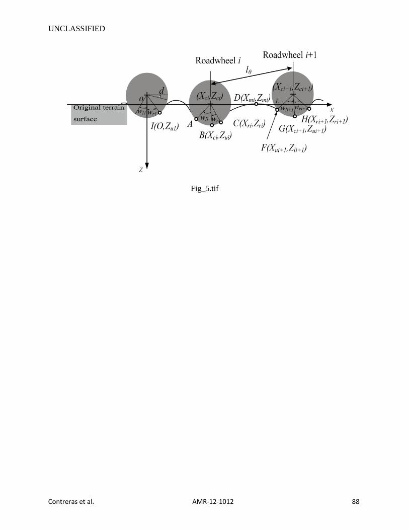
UNCLASSIFIED


Fig_5.tif

UNCLASSIFIED


Fig_6.tif

UNCLASSIFIED


Fig_7.tif

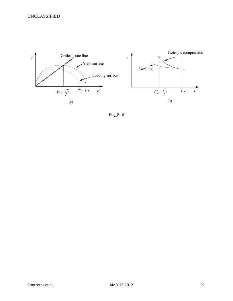
UNCLASSIFIED


Fig_8.tif

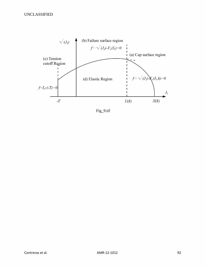
UNCLASSIFIED


Fig_9.tif

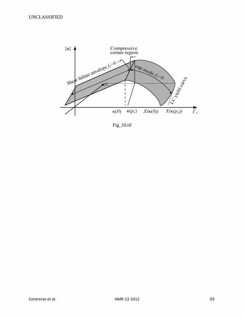
UNCLASSIFIED


Fig_10.tif

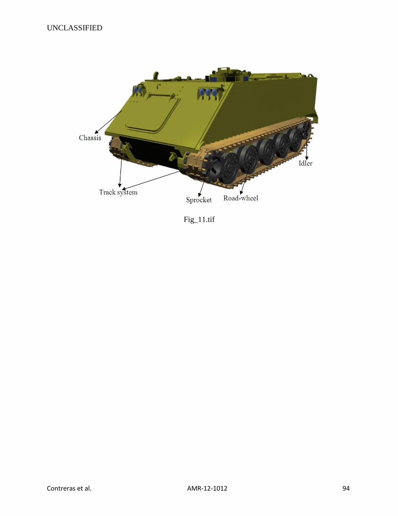
UNCLASSIFIED


Fig_11.tif

SOIL MODELS AND VEHICLE SYSTEM DYNAMICS · soil models and vehicle system dynamics ulysses...

Documents

Transcript of SOIL MODELS AND VEHICLE SYSTEM DYNAMICS · soil models and vehicle system dynamics ulysses...