Contents lists available at ScienceDirect

Soil Dynamics and Earthquake Engineering

journal homepage: www.elsevier.com/locate/soildyn

Prediction models and seismic hazard assessment: A case study from Taiwan

Yun Xua, J.P. Wangb,∗, Yih-Min Wuc, Hao Kuo-Chend

a Dept. Civil & Environmental Eng., Hong Kong University of Science and Technology, ChinabDept. Civil Engineering, National Central University, Taiwanc Dept. Geosciences, National Taiwan University, TaiwandDept. of Earth Sciences and Institute of Geophysics, National Central University, Taiwan

A R T I C L E I N F O

Keywords:CAVPrediction equationSeismic hazardTaiwan

A B S T R A C T

Proposed in the late 1980s, cumulative absolute velocity (CAV) is a new intensity measure for earthquakeground motion characterizations, followed by studies and applications such as CAV ground motion predictionequations (GMPEs). In this study, two new CAV GMPEs were developed with 24,667 strong-motion records fromTaiwan, and the first CAV seismic hazard assessment for Taipei (the most important city in Taiwan) was thenconducted using the local CAV models. It shows that the annual rate for the study area to encounter a groundmotion with CAV>0.97 g-sec is 0.002 per year, corresponding to a 10% occurrence probability in 50 years. Bycontrast, the deterministic scenario-based analysis shows that the CAV seismic hazard is about 0.60 g-sec for thestudy area. Future studies are worth conducting to develop more sophisticated, local CAV GPMEs and to exploremore applications of such CAV prediction models, such as the developments of PGA-CAV joint probabilitydistributions for conducting PGA-CAV joint seismic hazard assessments.

1. Introduction

Earthquakes generate random ground motions governed by avariety of uncertainties (e.g., source mechanisms, wave propagationpath, site condition, topography, etc.). In order to characterize the in-tensity of an earthquake, many intensity measures (IMs) were proposed[1], such as peak ground acceleration (PGA) and response spectral ac-celeration (SA) that are commonly used for earthquake-resistant design.For estimating the levels of PGA/SA during earthquakes, ground motionprediction equations (GMPEs) were developed and calibrated with in-strumental data [e.g., Refs. [2–7]]. For example, several PGA GMPEswere developed based on the NGA (Next Generation of Ground-MotionAttenuation Models) database [2–5], with others developed based onlocal data from Greece and Taiwan [6,7].

Proposed in the late 1980s, cumulative absolute velocity (CAV) is anew intensity measure for earthquake ground motion characterizations.Different from PGA/SA based on a motion’s peak amplitude only, CAVis a result of the whole acceleration time history that was first proposedby the Electric Power Research Institute (EPRI) to improve post-earth-quake inspection on nuclear power plants [8]. Specifically, the moti-vation was originated from realizing three nuclear power plants, whichwere nonoperational at that time, would had been requested a shut-down by U.S. Nuclear Regulatory Commission (USNRC) for post-earthquake inspection, even though the plants were clearly not

affected. For better addressing the issue, EPRI led a research projectstudying the correlation between structural damages and several IMs;then based on 250 earthquake records, CAV was found as the mostsuitable indicator/predictor to structural damage among the IMs ex-amined [8].

According to EPRI, the mathematical formulation of CAV was de-fined as follows [8]:

∫=CAV a t dt( )t

0

max

(1)

where a t( ) denotes the absolute value of acceleration at time t, andtmax is the duration of the ground motion. Fig. 1a illustrates the cal-culation of CAV for a hypothetical motion. As the shaded area shown,CAV is an intensity measure based on the whole acceleration timehistory, considering the cumulative effect of an earthquake groundmotion.

Later on, different versions of CAV were proposed for excludingCAV contributions from small amplitudes that are unlikely to causestructural damage [e.g., Refs. [9–11]]. For example, one derivative,referred to as CAVCUTOFF herein (Fig. 1b), is expressed as follows[9,10]:

∫∑= −=

=

+CAV H pga pga a t dt( ) | ( )|i

N

i t t

tCUTOFF

1cutoff

i

i 1

(2)

https://doi.org/10.1016/j.soildyn.2019.03.038Received 10 December 2018; Accepted 26 March 2019

∗ Corresponding author.E-mail address: jpwang@ncu.edu.tw (J.P. Wang).

Soil Dynamics and Earthquake Engineering 122 (2019) 94–106

0267-7261/ © 2019 Elsevier Ltd. All rights reserved.

T

where N is the total duration of a ground motion in seconds, pgai is themaximum acceleration (absolute value) in the i-th second of the motion,pgacutoff is the acceleration cutoff value, and H() is the Heavisidefunction:

= ⎧⎨⎩

≥>H x x

x( ) 1, 00, 0 (3)

Note that the cutoff thresholds of 0.025 g and 0.02 g were proposedin different studies [9,10].

Correlation between CAV and structural damage has been examinedsince then. EPRI found that CAV was a good indicator to ModifiedMercalli Intensity (MMI) VII, a level that damages on buildings of gooddesign starts to occur [8]. Similarly, Cabañas et al. [10] found a strongcorrelation between CAVCUTOFF = 0.02 g and the local macroseismic in-tensity in Italy, while Koliopoulos et al. [12] noted that CAV andHousner Intensity [13] were well correlated based on data from Greece.Then Kostov [14] concluded CAV should be a better indicator than PGAto structural damage, based on more instrumental data and field ob-servations. Moreover, Campbell and Bozorgnia further investigated thecorrelation between the standardized CAV and Japan MeteorologicalAgency (JMA) and MMI macroseismic intensity scales, characterizingthe thresholds of standardized CAV associated with the onsets of da-mage to structures of good design and construction, one of the im-portant findings and contributions from the study [15].

As PGA/SA GMPEs, several CAV models were developed for CAVpredictions. The models include those proposed by Danciu and Tselentis[6] based on data from Greece, and those by Campbell and Bozorgniaconsidering styles of faulting and rupture depth into their model de-velopment [16,17]. In addition, for increasing such a model’s applic-ability Du and Wang [18] developed a CAV GMPE in a simpler func-tional form. Notably, it has been consistently pointed out that thestandard deviation of CAV GMPEs is smaller than that of a series ofGMPEs for PGA, SA, AI (Arias Intensity), etc., even developed with thesame functional form and the same pool of earthquake data [e.g., 6,19].

Although several CAV GMPEs as mentioned above have been

proposed and local PGA GMPEs have been developed for the area ofTaiwan [7], not a local CAV model was developed for the area. As aresult, the key scope of the study is to develop the first CAV GMPEs forTaiwan. Specifically, the data from the Taiwan Strong Motion In-strumentation Program (TSMIP) were collected and used. We alsoconducted the first CAV seismic hazard study for Taipei (the most im-portant city in Taiwan) using the CAV models developed, anotherhighlight and contribution of the study.

2. Taiwan Strong Motion Instrumentation Program, TSMIP

2.1. Overview

Located on the boundaries of three tectonic plates, the regionaround Taiwan is known for high seismicity. Statistics show that around2,000 earthquakes above ML 3.0 (local magnitude) can be occurring inthe region every year, and a catastrophic event like the ML 7.3 Chi-Chiearthquake in 1999 could recur in decades [20]. As a result, a variety ofearthquake studies, such as earthquake early warning [e.g., Ref. [21]],seismic hazard analysis [e.g., Refs. [22,23]], and earthquake prob-ability evaluation [e.g., Refs. [24–26]], were conducted for the regionaround Taiwan.

In order to gather more seismic data, the Taiwan Strong MotionInstrumentation Program, TSMIP, was launched in the 1990s, buildingmany earthquake stations in order to collect ground motion data. As ofnow, TSMIP has 688 free-field earthquake stations in operation [27],with each capable of recording ground motions in three directions witha sampling rate of 200 or 250 per second [28]. It is also worth notingthat around 100 stations among them are equipped with automatic datatransmitting systems that can send data to the Central Weather BureauTaiwan immediately for some real-time analyses, like earthquake earlywarning [29].

Based on the NEHRP (National Earthquake Hazards ReductionProgram) provisions, 439 of the stations were investigated and cate-gorized into one of the following site conditions: 1) Type A: hard-rocksite with Vs30 > 1500m/s, where Vs30 is the average shear-wave

Fig. 1. CAV (cumulative absolute velocity) of a hypothetical acceleration time history that is equal to the summation of the shaded area: a) CAV and b) CAVCUT-

OFF= 0.025 g.

Y. Xu, et al. Soil Dynamics and Earthquake Engineering 122 (2019) 94–106

95

velocity in the top 30m below the ground surface; 2) Type B: firm-tohard-rock site with Vs30 from 760 to 1500m/s; 3) Type C: dense-soiland soft-rock site with Vs30 from 360 to 760m/s; 4) Type D: stiff-soilsite with Vs30 ranging from 180 to 360m/s; and 5) Type E: soft-soil sitewith Vs30 < 180m/s. Fig. 2 shows the distribution of the 439 stationswith known site conditions. For more details on the site investigationsand characterizations, refer to Kuo et al. [30].

The TSMIP database becomes invaluable to earthquake studies,especially those focusing on Taiwan. For example, Sokolov et al. [31]used the local database to investigate the basin effect in Taipei on siteamplification during earthquakes. For earthquake early warning, the“high-density” instrumental network is the key to the success of a localsystem that can issue warnings as soon as 20 s after the occurrence/initiation of earthquake [32]. Moreover, the database also providesopportunities for cross-checking the earthquake models that have beendeveloped. For instance, Xu et al. [33] reported that the reliability of anon-site earthquake early warning implemented in Taiwan was around85%, calculated by counting the numbers of missed alarm and falsealarm based on 40,000 plus tests using TSMIP ground motions sub-stituted into the decision-making criteria. Other TSMIP-based studiesinclude local ground motion model developments [7] and earthquakestatistical study for Taiwan [34].

2.2. Data collection and processing

Since the 1990s, TSMIP has recorded a lot of (raw) data in theformat of acceleration time histories. As a result, our first task is togather the data of our interest under following conditions: 1) motionsfrom stations with known site conditions were collected for in-corporating site effect into model developments; 2) motions associatedwith magnitude above Mw 4.8 (moment magnitude) and within 200 kmfrom epicenters were collected, screening out less severe motions thatare incapable of causing structure damage. Therefore, a total of 24,667strong-motion data were collected from the local database, and it is thelargest sample size by far for a GMPE study, to the best of our knowl-edge.

More details regarding the data set are as follows: 1) the 24,677records are associated with 310 major earthquakes (moment magnitude

Fig. 2. Spatial distribution of the 439 classified stations of the Taiwan StrongMotion Instrumentation Program (TSMIP) ([28]).

Fig. 3. Moment magnitude and epicentral distance of the 24,677 local strong-motion data used in this study: a) Type-B site condition, b) Type-C site condition, c)Type-D site condition, and d) Type-E site condition; note that the shallow-source and deep-source data are separated by a focal depth of 30 km.

Y. Xu, et al. Soil Dynamics and Earthquake Engineering 122 (2019) 94–106

96

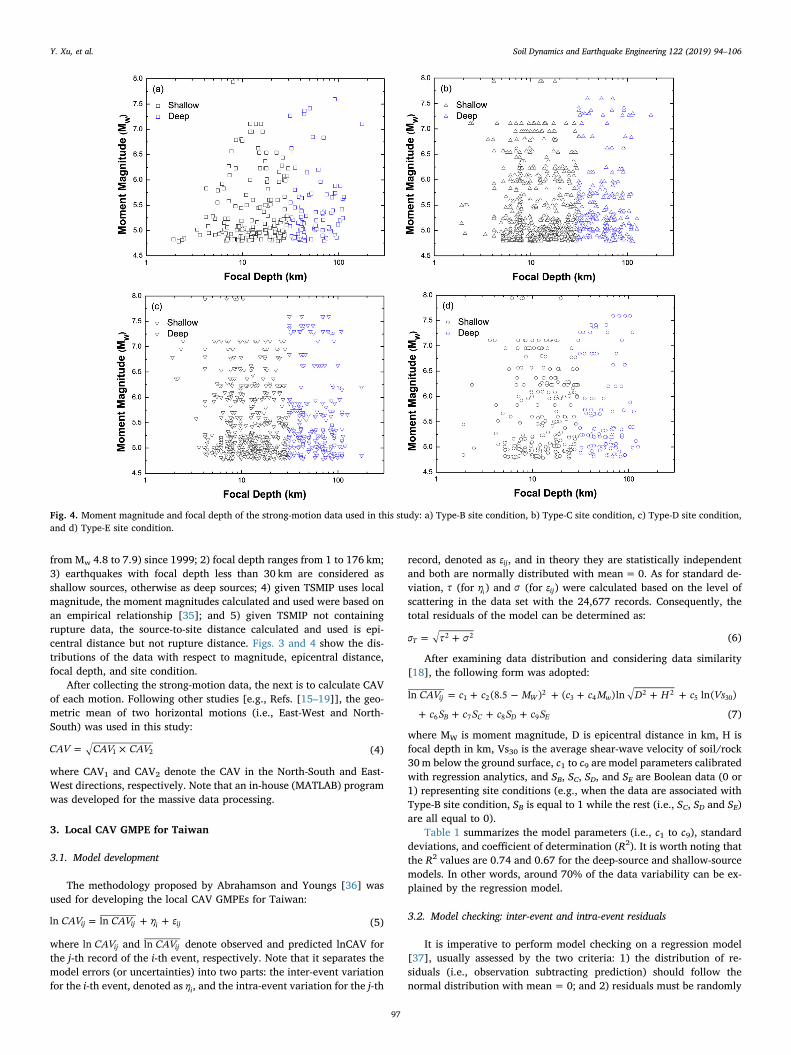
from Mw 4.8 to 7.9) since 1999; 2) focal depth ranges from 1 to 176 km;3) earthquakes with focal depth less than 30 km are considered asshallow sources, otherwise as deep sources; 4) given TSMIP uses localmagnitude, the moment magnitudes calculated and used were based onan empirical relationship [35]; and 5) given TSMIP not containingrupture data, the source-to-site distance calculated and used is epi-central distance but not rupture distance. Figs. 3 and 4 show the dis-tributions of the data with respect to magnitude, epicentral distance,focal depth, and site condition.

After collecting the strong-motion data, the next is to calculate CAVof each motion. Following other studies [e.g., Refs. [15–19]], the geo-metric mean of two horizontal motions (i.e., East-West and North-South) was used in this study:

= ×CAV CAV CAV1 2 (4)

where CAV1 and CAV2 denote the CAV in the North-South and East-West directions, respectively. Note that an in-house (MATLAB) programwas developed for the massive data processing.

3. Local CAV GMPE for Taiwan

3.1. Model development

The methodology proposed by Abrahamson and Youngs [36] wasused for developing the local CAV GMPEs for Taiwan:

= + +CAV CAV η εln lnij ij i ij (5)

where CAVln ij and CAVln ij denote observed and predicted lnCAV forthe j-th record of the i-th event, respectively. Note that it separates themodel errors (or uncertainties) into two parts: the inter-event variationfor the i-th event, denoted as ηi, and the intra-event variation for the j-th

record, denoted as εij, and in theory they are statistically independentand both are normally distributed with mean= 0. As for standard de-viation, τ (for ηi) and σ (for εij) were calculated based on the level ofscattering in the data set with the 24,677 records. Consequently, thetotal residuals of the model can be determined as:

= +σ τ σT2 2 (6)

After examining data distribution and considering data similarity[18], the following form was adopted:

= + − + + + +

+ + + +

CAV c c M c c M D H c Vs

c S c S c S c S

ln (8.5 ) ( )ln ln( )ij W w

B C D E

1 22

3 42 2

5 30

6 7 8 9 (7)

where MW is moment magnitude, D is epicentral distance in km, H isfocal depth in km, Vs30 is the average shear-wave velocity of soil/rock30m below the ground surface, c1 to c9 are model parameters calibratedwith regression analytics, and SB, SC, SD, and SE are Boolean data (0 or1) representing site conditions (e.g., when the data are associated withType-B site condition, SB is equal to 1 while the rest (i.e., SC, SD and SE)are all equal to 0).

Table 1 summarizes the model parameters (i.e., c1 to c9), standarddeviations, and coefficient of determination (R2). It is worth noting thatthe R2 values are 0.74 and 0.67 for the deep-source and shallow-sourcemodels. In other words, around 70% of the data variability can be ex-plained by the regression model.

3.2. Model checking: inter-event and intra-event residuals

It is imperative to perform model checking on a regression model[37], usually assessed by the two criteria: 1) the distribution of re-siduals (i.e., observation subtracting prediction) should follow thenormal distribution with mean= 0; and 2) residuals must be randomly

Fig. 4. Moment magnitude and focal depth of the strong-motion data used in this study: a) Type-B site condition, b) Type-C site condition, c) Type-D site condition,and d) Type-E site condition.

Y. Xu, et al. Soil Dynamics and Earthquake Engineering 122 (2019) 94–106

97

distributed with little correlation with prediction variables. With thetwo criteria verified, the regression model is then considered robust.

Figs. 5 and 6 show the inter-event residuals with respect to mag-nitude and focal depth (two key independent variables of the regressionmodel). It was found that the residuals are randomly distributed withlittle correlation with either magnitude or depth. Figs. 7–9 show theintra-event residuals against magnitude, epicentral distance and Vs30,with little correlation found either. Figs. 10 and 11 are the histogramsof the residuals, demonstrating a bell-shaped distribution well simu-lating the normal distribution targeted. Therefore, the regressionmodels should be robust based on the diagnostic plots, with residualsshowing little correlation with independent variables and their dis-tribution close to the normal distribution.

4. Model evaluation and comparison

Figs. 12–14 show the medians of CAV with respect to site condition,epicentral distance, and moment magnitude. It shows that the shallow-source model consistently predicts a greater CAV than the deep-sourcemodel does. In addition, as shown in Fig. 12, larger predictions appearas far as the Type-E site condition is concerned, followed by motions onType-D, Type-C, and Type-B site conditions, revealing softer materialscould amplify earthquake motions more extensively. For shallow-source models subject to Mw 6.5 as shown in Fig. 12a, CAV predictionsattenuate nonlinearly with increasing distance; by contrast, the CAVpredictions from the deep-source model shown in Fig. 12b are somehowsaturated till 30 km from the epicenter, then attenuating more linearlywith distance increasing from 30 km. On the condition of strong ground

Table 1Summary of the two CAV GMPEs for Taiwan developed with the TSMIP database.

Earthquake Source Model parameters τa σb Rb Sample size

c1 c2 c3 c4 c5 c6 c7 C8 c9

Shallow 1.153 −0.117 −1.565 0.127 −0.114 0.465 0.978 1.245 1.465 0.335 0.475 0.67 17,171Deep 0.974 0.064 −2.873 0.309 −0.208 1.087 1.485 1.542 1.467 0.187 0.485 0.74 7,496

a τ is the standard deviation of the inter-event residual, and.b σ is the standard deviation of the intra-event residual.

Fig. 5. Distribution of inter-event residuals against moment magnitude: a)shallow sources and b) deep sources.

Fig. 6. Distribution of inter-event residuals against focal depth: a) shallowsources and b) deep sources.

Y. Xu, et al. Soil Dynamics and Earthquake Engineering 122 (2019) 94–106

98

shaking resulting from small source-to-site distance (e.g., < 30 km) andlarge magnitude (e.g., Mw > 6.5), the shallow-source model has thefeature that the CAV increment because of site condition is nearly aconstant, unlike the deep-source model that shows a large incrementfrom Site B to Site C, while the site effect is almost saturated from a softsite (Site D) to a very soft site (Site E). Such features present in the CAVGMPEs are quite unique in comparison to models developed byCampbell and Bozorgnia [16,19] identifying CAV predictions could beamplified with site condition in a more nonlinear nature, but similar tothe model developed by Du and Wang [18]. It is postulated that thedifference in site amplification effect should be resulted from theadopted functional forms. More sophisticated functional forms couldpossibly capture more detailed site behavior, however, limiting themodel’s applicability. More studies are worth conducting to investigatethe possible causes to such features present in the local model. On theother hand, owing to the uniqueness of a local model reflecting to theunique local geological background, it is better and more reasonable toadopt local models in follow-up applications to make the results morerepresentative, which is also the key motivation of the study to developthe first CAV GMPE based on local data.

On the basis of using similar functional forms for the model devel-opments, the model developed in this study, referred to as Model 2017,was first compared to the reference model referred to as Model 2012[18]. The act is to provide some more justification to the new, local

models for Taiwan that are able to predict CAV reasonably. However,the four underlying differences between the two must be noted becauseof the different formats in raw data: i) Model 2017 incorporates focaldepth and Vs30 in model development; ii) Model 2017 incorporates theType-B and Type-E site conditions; iii) Model 2017 uses epicentraldistance; iv) Model 2017 does not incorporate styles of faulting.

Fig. 15 shows CAV predictions from the two models. In terms of thecentral value, overall Model 2012 predicts a greater CAV than Model2017 does. Since earthquake induced ground motions are strongly in-fluenced by focal depth and rupture direction (especially for nearsource and a major event), this difference should result from the factsthat we used epicentral distance and did not account for faulting me-chanisms in the model. However, this is the limitation that the TSMIPground-motion database does not have rupture data and detailed focalmechanisms as mentioned previously. But overall speaking (fromFig. 15a–c), the CAV predictions from the two models are comparable,providing additional verification to the local model that predicts CAVreasonably.

Moreover, Model 2017 was further compared to the CAV GMPEdeveloped by Campbell and Bozorgnia [19] based on NGA database.Note that the model development of the Campbell and Bozorgnia’smodel, referred to as Model 2010, is quite different and sophisticated,incorporating effect of fault mechanism, hanging wall, shallow siteresponse, and basin effect. The comparison, as shown in Fig. 16,

Fig. 7. Distribution of intra-event residuals against moment magnitude: a)shallow sources and b) deep sources. Fig. 8. Distribution of intra-event residuals against epicentral distance: a)

shallow sources and b) deep sources.

Y. Xu, et al. Soil Dynamics and Earthquake Engineering 122 (2019) 94–106

99

indicates a larger estimate from Model 2010 than Model 2017. How-ever, again, median estimates of CAV and the trend of CAV estimatesare generally in agreement with each other. Considering very differentdatabase and different functional forms in the model development ofModel 2010 and Model 2017, the difference in CAV predictions shouldbe reasonable and acceptable.

In terms of aleatory uncertainty, Model 2017 has a larger standarddeviation than Model 2012, or Model 2010, does. The possibilities tothe result and the difference could be as follows: 1) epicentral distanceused in Model 2017 could be less indicative to ground motion thanrupture distance; 2) the ground motions used for developing Model2017 are more diversified, including those associated with earthquakesin subduction zones of northeastern and southwestern Taiwan, andthose from other geological regimes in central and western Taiwan; 3)an empirical relationship was used to convert local magnitude to mo-ment magnitude, an additional source of uncertainty to Model 2017;and 4) the nature of ground motion attenuation in Taiwan is morerandom than other areas, probably owing to a more complicated geo-logical background.

Based on the residual plots and the model comparison, the localCAV GMPE for Taiwan is considered mathematically robust, and cap-able of producing reasonable predictions as the reference. Future stu-dies are worth investigating to compare it with more CAV GMPEs, al-though the comparison might be somewhat ambiguous if model basics

are fundamentally different (e.g., epicentral distance vs rupture dis-tance). To better address this, TSMIP is better to include rupture dataand other focal mechanisms (especially for major events) in the future,so that new local models based on different formats of data can befurther developed.

5. Discussion

5.1. Seismic hazard analysis

Seismic hazard analysis has become more important to (site-spe-cific) earthquake-resistant design. On top of case studies [e.g., Refs.[38–44]], technical references, such as R.G. 1.208 of U.S. NuclearRegulatory Commission (USNRC) [45], have prescribed it as the stan-dard method for developing site-specific design parameters for nuclearpower plants. Seismic hazard analysis can be mainly categorized intoProbabilistic Seismic Hazard Analysis (PSHA) and DeterministicSeismic Hazard Analysis (DSHA) [46]. It is noted that “seismic hazard”is referred to as “the likelihood of experiencing a specified intensity of anydamaging phenomenon at a particular site” [47,48], instead of economicloss or loss of life implicated from hazard.

• Overview of PSHA

The methodology and algorithm of PSHA can be summarized as

Fig. 9. Distribution of intra-event residuals against Vs30: a) shallow sourcesand b) deep sources.

Fig. 10. Normal plot of inter-event and intra-event residuals from shallowsources: a) inter-event residual and b) intra-event residual.

Y. Xu, et al. Soil Dynamics and Earthquake Engineering 122 (2019) 94–106

100

follows: The performance function of the probabilistic analysis isusually a PGA or SA GMPE as PGA = f (M, D) + ε, where ε is themodel’s standard deviation (M is magnitude, and D is distance). Thenthe analysis is to estimate the exceedance probability of a certain levelof ground shaking that a site would encounter, based on the un-certainties associated with the three variables (i.e., ε, M, and D). Notethat PSHA uses total-probability algorithms as follows to calculate theexceedance Pr(PGA > y*) [1], which can also be solved using MonteCarlo Simulation [49,50].

∑ ∑> ∗ = > ∗ = = × =

× =

= =PGA y PGA y D d M m D d

M m

Pr( ) Pr( | , ) Pr( )

Pr( )

i

N

j

N

i j i

j

1 1

D M

(8)

where NM and ND are the number of data bins in magnitude and dis-tance probability functions as shown in Fig. 17a and b.

Fig. 17 is a systematic diagram showing the basics of PSHA com-putation: For a given magnitude and distance, the probability dis-tribution of lnPGA (or PGA) can be estimated with a GMPE, so that theexceedance probability Pr(PGA > y*) can be calculated as the high-lighted area in Fig. 17c. With such calculation repeated using differentmagnitudes and distances with their probabilities also characterized(i.e., Fig. 17a and b), the total exceedance probability Pr(PGA > y*) isthen equal to the sum of exceedance probabilities associated with eachscenario, as the equation expressed in Eq. (8).

The total exceedance probability calculated with Eq. (8) is seismichazard contributed by one earthquake from one specific seismic zone.Therefore, when a site is surrounded by NS sources with each’s annualrate= v, the annual rate for the site to encounter a ground motion withPGA > y*, denoted as > ∗λ PGA y( ), becomes as follows [1]:

∑> ∗ = × > ∗=

λ PGA y v PGA y( ) Pr( )k

N

k1

S

(9)

To sum up, PSHA is a probabilistic analysis to estimate the annualrate of PGA exceedance considering the (aleatory) uncertainties ofearthquake magnitude, location, and GMPE model error. The perfor-mance function is a PGA (or SA) GMPE, and the calculation is usuallysolved by using total-probability algorithms.

• Overview of DHSA

Deterministic Seismic Hazard Analysis, or scenario-based analysis,is relatively straightforward compared to PSHA. Different than PSHAconsidering magnitude and distance uncertainties, DSHA estimatesseismic hazard subject to a worst-case scenario in term of (maximum)magnitude and (minimum) distance. Therefore, for a given PGA GMPEas PGA= f (M, D) ± σε, the deterministic estimates from DSHA are

Fig. 11. Normal plot of inter-event and intra-event residuals from deep sources:a) inter-event residual and b) intra-event residual.

Fig. 12. Median predicted values of CAV with respect to site condition: a)shallow source and b) deep source; note that the median predicted CAV value iscalculated with MW=6.5; Note that the focal depth for shallow and deepsource is assumed to be 15 km and 75 km, respectively, and the Vs30 for site B,C, D, E is assumed to be 906, 512, 233, and 158m/s, respectively.

Y. Xu, et al. Soil Dynamics and Earthquake Engineering 122 (2019) 94–106

101

equal to PGA= f (Mmax, Dmin), with some recommending it as PGA= f(Mmax, Dmin) + σε with the standard deviation of model error (σε) alsotaken into account.

Then when a site is surrounded by NS seismic sources, the maximumof the NS deterministic seismic hazards is the final estimate of DSHA[1]:

=PGA MAX PGA{ }i (10)

where PGAi is the deterministic seismic hazard associated with the i-thseismic source.

• Issues with seismic hazard assessment

It is understood that neither PSHA nor DSHA could perfectly predictseismic hazards [e.g., Refs. [51–56]]. It was found that PSHA predic-tions were quite deviated from our instrumental data/observation [52],while DSHA might underestimate seismic hazard without consideringthe aleatory uncertainty of a GMPE model [54]. Others include proper/improper use of logic-tree analysis in seismic hazard analysis, and theissue with the assessment’s transparency and repeatability, amongothers [57,58]. The comments summarized here should provide a morecomplete review on seismic hazard analysis, while it is beyond thescope of this study to justify each of them.

5.2. CAV seismic hazard study for Taipei

As mentioned previously, most seismic hazard studies are PGA- orSA-based using associated GMPEs as the performance function.Therefore, one application of the CAV GMPEs we developed is CAVseismic hazard assessment, estimating the annual rate of CAV ex-ceedance from probabilistic analysis, or the maximum CAV from de-terministic analysis. Compared to conventional seismic hazard assess-ments, the modification is to replace PGA GMPEs with CAV ones.

With the local CAV GMPE and with other seismological/geologicaldata from the literature (i.e., Fig. 18: local seismic source models;Table 2: data summary) [59], we conducted the first CAV seismic ha-zard analysis for a typical site (121.51°E and 25.03°N; Type-E condition;Vs30=160m/s) in Taipei. Fig. 19 shows the CAV hazard curve for thesite, with an annual rate of CAV>0.97 g-sec about 0.002 per year, orthere is a 10% occurrence probability for Taipei to encounter suchseismic hazard in 50 years. By contrast, the analysis also suggests anannual rate of 0.078 per year that the city could experience such aseismic hazard. Note that CAV>0.30 g-sec is considered the thresholdof MMI level VII [8].

On the other hand, the DSHA estimate is about 0.60 g-sec in CAV forTaipei, on the basis of the maximum magnitude and minimum distance.More details of the analysis (e.g., maximum earthquake magnitude andshortest epicentral distance of each seismic source) are summarized inTable 3.

Fig. 13. Median predicted values of CAV with respect to epicentral distance: a)shallow source and b) deep source; note that median predicted CAV value iscalculated for Type-D site condition with the Vs30= 233m/s.

Fig. 14. Median predicted values of CAV with respect to moment magnitude: a)shallow source and b) deep source; note that median predicted CAV value iscalculated for Type-D site condition with the Vs30=233m/s.

Y. Xu, et al. Soil Dynamics and Earthquake Engineering 122 (2019) 94–106

102

Fig. 15. Comparison between Model 2017 (this study) and Model 2012: a)median values calculated for different site condition given MW=7, b) medianvalues calculated given different moment magnitude for Type-C site condition,and c) median values calculated given different epicentral distance for Type-Csite condition; note that Vs30= 906, 512, 233, 158m/s is adopted for Type-B,C, D, E site condition, respectively, in Mode 2017, and median values of Model2012 are calculated referring to normal faulting.

Fig. 16. Comparison between Model 2017 (this study) and Model 2010. Unlessotherwise specified, median values are evaluated with MW=7, normalfaulting, Vs30= 906, 512, 233, 158m/s for Type-B, C, D, E site condition, re-spectively, Z2.5= 2 km, ZTOR= 10 km, RRUP= 2RJB, |δ|≤ °70

Y. Xu, et al. Soil Dynamics and Earthquake Engineering 122 (2019) 94–106

103

5.3. PGA-CAV joint seismic hazard assessment and future study

To the best of our knowledge, not an earthquake-resistant designuses CAV as the only criterion to design/build structures capable of

withstanding ground motions with CAV>0.16, g-sec, 0.3 g-sec, etc. Asa result of that, it requires more future studies to explore how to im-plement CAV seismic hazard analysis into earthquake-resistant design,as some studies pointed out [60–63].

Fig. 17. Systematic diagram illustrating the basics of PSHA algorithms: a)distribution of source-to-site distance, b) distribution of magnitude, and c)lnPGA distribution from GMPE under a given magnitude and distance, and theexceedance probability as the shaded area.

Fig. 18. Locations of the study site (121.51°E, 25.03°N) and the 12 seismicsources within 200 km from the site [59].

Table 2Summary of the 12 area sources within 200 km from the study site; the a-valueand b-value are the parameters of the Gutenberg-Richter recurrence law ([59]).

Source zone a-value b-value Maximum magnitude (Mw)

A 3.100 0.849 6.6B 2.579 0.800 6.4C 3.137 0.916 5.0D 3.118 0.740 6.5E 1.914 0.577 6.5F 2.163 0.689 6.5G 2.236 0.638 6.5H 2.453 0.593 7.6I 3.270 0.658 7.6J 3.249 0.644 7.0K 1.943 0.520 6.5L 2.962 0.681 7.5

Fig. 19. CAV seismic hazard curve for Taipei (121.51°E and 25.03°N; Type-Esite condition; Vs30=160m/s).

Y. Xu, et al. Soil Dynamics and Earthquake Engineering 122 (2019) 94–106

104

For example, PGA-CAV joint (probabilistic) seismic hazard assess-ment that calculates the PGA-CAV exceedance probability, Pr(PGA > pga* and CAV > cav*), is considered an improvement overthe conventional PGA- or SA-based approach. Specifically, EPRI pro-posed CAV 0.16 g-sec as a threshold for such PGA-CAV joint assess-ments that aim to estimate the annual rate of PGA > pga* andCAV>0.16 g-sec with the additional criterion (i.e., CAV > 0.16 g-sec). In addition, the correlation between CAV and PGA/SA was alsoinvestigated, which should help select/develop site-specific groundmotions for some earthquake-resistant design [62].

Theoretically speaking, the PGA-CAV joint seismic hazard studyshould not be that difficult to be implemented because the methodologyis the almost same as the conventional assessment. The key technicalissue is how to develop PGA-CAV joint probability distributions subjectto a given pair of magnitude and distance. Although some “prototype”methods were proposed for resolving the calculation, more justificationwith field data is need [e.g., 60, 63].

We also consider the PGA-CAV seismic hazard study should bebetter than the current model, and the methodology is worth studyingin the future. Recently, it was found that PGA-CAV joint probabilityfunctions can be well modeled by the copula theory/approach [34], andthis could be useful to the developments of PGA-CAV joint probabilitydistributions, then facilitating PGA-CAV seismic hazard assessments.

6. Summary

Based on data from a local strong-motion database in Taiwan, thisstudy developed the first local CAV GMPEs for the study area, includingmodel checking and model comparison. Also note that the empiricalmodel developed was based on 24,667 strong-motion records, the lar-gest sample size by far for such a study.

The paper also presents the first CAV seismic hazard assessment forTaipei, using the local CAV GMPE we developed. The probabilisticanalysis shows that the annual rate for the city to encounter a groundmotion with CAV>0.97 g-sec is about 0.002 per year, or there is a 10%occurrence probability for such a seismic hazard to recur in 50 years. Bycontrast, the deterministic, scenario-based analysis suggests the CAVestimate be 0.60 g-sec for the study area.

Acknowledgements

We appreciate the Editor and the reviewer for the review and con-structive comments, making the submission much improved in so manyaspects. We are thankful to the Central Weather Bureau Taiwan forproviding data for this study. We also appreciate the financial supportfrom the Ministry of Science and Technology, Republic of China

(Taiwan) on this research (Grant: MOST106-2218-E-008-013-MY2).

References

[1] Kramer SL. Geotechnical earthquake engineering. N. J.: Prentice Hall Inc.; 1996.[2] Abrahamson N, Silva W. Summary of the Abrahamson & silva NGA ground-motion

relations. Earthq Spectra 2008;24:67–97.[3] Boore DM, Atkinson GM. Ground-motion prediction equations for the average

horizontal component of PGA, PGV, and 5%-damped PSA at spectral periods be-tween 0.01 s and 10.0 s. Earthq Spectra 2008;24:99–138.

[4] Campbell KW, Bozorgnia Y. NGA ground motion model for the geometric meanhorizontal component of PGA, PGV, PGD and 5% damped linear elastic responsespectra for periods ranging from 0.01 to 10 s. Earthq Spectra 2008;24:139–71.

[5] Chiou BJ, Youngs RR. An NGA model for the average horizontal component of peakground motion and response spectra. Earthq Spectra 2008;24:173–215.

[6] Danciu L, Tselentis G. Engineering ground-motion parameters attenuation re-lationships for Greece. Bull Seismol Soc Am 2007;97:162–83.

[7] Lin PS, Lee CT, Cheng CT, Sung CH. Response spectral attenuation relations forshallow crustal earthquakes in Taiwan. Eng Geol 2011;121:150–64.

[8] Electric Power Research Institute (EPRI). A criterion for determining exceedance ofthe operating basis earthquake. Report NP-5930, Palo Alto, California. 1988.

[9] Electric Power Research Institute (EPRI). Standardization of the cumulative abso-lute velocity. Report TR-100082, Palo Alto, California. 1991.

[10] Cabañas L, Benito B, Herráiz M. An approach to the measurement of the potentialstructural damage of earthquake ground motions. Earthq Eng Struct Dyn1997;26:79–92.

[11] Kramer SL, Mitchell RA. Ground motion intensity measures for liquefaction hazardevaluation. Earthq Spectra 2006;22:413–38.

[12] Koliopoulos PK, Margaris BN, Klimis NS. Duration and energy characteristics ofGreek strong motion records. J Earthq Eng 1998;2:390–417.

[13] Housner GW. Behavior of structures during earthquakes. J Eng Mech Div ASCE1959;85:104–29.

[14] Kostov M. Site specific estimation of cumulative absolute velocity. Proceeding of18th international conference on structural mechanics in reactor technology.Beijing, China: SMiRT 18; 2005. p. 3041–50.

[15] Campbell KW, Bozorgnia Y. Cumulative absolute velocity (CAV) and seismic in-tensity based on the PEER-NGA database. Earthq Spectra 2012;28:457–85.

[16] Campbell KW, Bozorgnia Y. A ground motion prediction equation for the horizontalcomponent of cumulative absolute velocity (CAV) based on the PEER-NGA strongmotion database. Earthq Spectra 2010;26:635–50.

[17] Campbell KW, Bozorgnia Y. Prediction equations for the standardized version ofcumulative absolute velocity as adapted for use in the shutdown of US nuclearpower plants. Nucl Eng Des 2011;241:2558–69.

[18] Du W, Wang G. A simple ground‐motion prediction model for cumulative absolutevelocity and model validation. Earthquake Eng Struc 2013;42:1189–202.

[19] Campbell KW, Bozorgnia Y. A comparison of ground motion prediction equationsfor Arias intensity and cumulative absolute velocity developed using a consistentdatabase and functional form. Earthq Spectra 2012;28:931–41.

[20] Wang JP, Wu YM. A new seismic hazard analysis using FOSM algorithms. SoilDynam Earthq Eng 2014;67:251–6.

[21] Hsiao NC, Wu YM, Zhao L, Chen DY, Huang WT, Kuo KH, Shin TC, Leu PL. A newprototype system for earthquake early warning in Taiwan. Soil Dynam Earthq Eng2011;31:201–8.

[22] Wang JP, Huang D, Yang Z. The deterministic seismic hazard map for Taiwan de-veloped using an in-house Excel-based program. Comput Geosci 2012;48:111–6.

[23] Wang JP, Huang D, Cheng CT, Shao KS, Wu YC, Chang CW. Seismic hazard analysisfor Taipei City including deaggregation, design spectra, and time history with Excelapplications. Comput Geosci 2013;52:146–54.

[24] Wu YM, Chen CC. Seismic reversal pattern for the 1999 Chi-Chi, Taiwan, Mw 7.6earthquake. Tectonophysics 2007;429:125–32.

[25] Wu YM, Chen CC, Zhao L, Chang CH. Seismicity characteristics before the 2003Chengkung, Taiwan earthquake. Tectonophysics 2008;457:177–82.

[26] Chen CH, Wang JP, Wu YM, Chan CH, Chang CH. A study of earthquake inter-occurrence times distribution models in Taiwan. Nat Hazards 2013;69:1335–50.

[27] Central CWB. Weather Bureau Taiwan. Available from: http://www.cwb.gov.tw/V7/earthquake/accsta.htm, Accessed date: April 2016.

[28] Shin TC, Tsai YB, Yeh YT, Liu CC, Wu YM. Strong-motion instrumentation programsin Taiwan. International Handbook of Earthquake and Engineering Seismology2003;81B:1057–62.

[29] Wen KL, Shin TC, Wu YM, Hsiao NC, Wu BR. Earthquake early warning technologyprogress in Taiwan. J Disaster Res 2009;4:202–10.

[30] Kuo CH, Wen KL, Hsieh HH, Lin CM, Chang TM, Kuo KW. Site classification andVs30 estimation of free-field TSMIP stations using the logging data of EGDT. EngGeol 2012;129–130:68–75.

[31] Sokolov VY, Loh CH, Wen KL. Empirical models for site and region-dependentground-motion parameters in the Taipei area: a unified approach. Earthq Spectra2001;17:313–31.

[32] Wu YM, Teng TL, Hsiao NC, Chin TC, Lee WHK, Tsai YB. Progress on earthquakerapid reporting and early warning systems in Taiwan. Earthquake hazard, risk, andstrong ground motion. Beijing: Seismological Press; 2004. p. 463–86.

[33] Xu Y, Wang JP, Wu YM, Kuo-Chen H. Reliability assessment on earthquake earlywarning: a case study from Taiwan. Soil Dynam Earthq Eng 2017;92:397–407.

[34] Xu Y, Tang XS, Wang JP, Kuo‐Chen H. Copula‐based joint probability function forPGA and CAV: a case study from Taiwan. Earthq Eng Struct Dyn 2016;13:2123–36.

[35] Wu YM, Shin TC, Chang CH. Near real-time mapping of peak ground acceleration

Table 3Summary of the deterministic CAV hazard assessment for the study site atTaipei; note that the site is located within Zone H and the focal depth is as-sumed at 15 km.

Source zone Maximumearthquakemagnitude (MW)

Shortestepicentraldistance (km)

Deterministic estimateof CAV (g-sec)

A 6.6 28.80 0.322B 6.4 0.00 0.480C 5.0 28.50 0.058D 6.5 98.89 0.128E 6.5 38.28 0.247F 6.5 36.89 0.253G 6.5 28.34 0.297H 7.6 38.80 0.600I 7.6 95.45 0.362J 7.0 64.83 0.278K 6.5 65.49 0.172L 7.5 102.41 0.320

Y. Xu, et al. Soil Dynamics and Earthquake Engineering 122 (2019) 94–106

105

and peak ground velocity following a strong earthquake. Bull Seismol Soc Am2001;91:1218–28.

[36] Abrahamson A, Youngs RR. A stable algorithm for regression analyses using therandom effects model. Bull Seismol Soc Am 1992;82:505–10.

[37] Devore JL. Probability and statistics for engineering and the science. Brooks/Cole,Cengage Learning; 2012.

[38] Wang JP, Xu Y, Wu YM. A FOSM calculation for seismic hazard assessment with theconsideration of uncertain size conversion. Nat Hazard Earth Sys 2013;13:2649–57.

[39] Mualchin L. Seismic hazard analysis for critical infrastructures in California. EngGeol 2005;79:177–84.

[40] Cheng CT, Chiou SJ, Lee CT, Tsai YB. Study on probabilistic seismic hazard maps ofTaiwan after Chi-Chi earthquake. J GeoEng 2007;2:19–28.

[41] Aldama-Bustos G, Bommer JJ, Fenton CH, Stanford PJ. Probabilistic seismic hazardanalysis for rock sites in the cities of Abu Dhabi, Dubai and Ra's Al Khaymah, UnitedArab Emirates. Georisk 2009;3:1–29.

[42] Roshan AD, Basu PC. Application of PSHA in low seismic region: a case study onNPP site in peninsular India. Nucl Eng Des 2010;240:3443–54.

[43] Sitharam TG, Kolathayar S. Seismic hazard analysis of India using areal sources. JAsian Earth Sci 2013;62:647–53.

[44] Wang JP, Taheri H. A seismic hazard analysis for the region of Tehran. Nat HazardsRev ASCE 2014;15:121–7.

[45] United States Nuclear Regulatory Commission (USNRC). Identification and char-acterization of seismic sources and determination of safe shutdown earthquakeground motion. Regulatory Guide 1997;1. 165.

[46] Graves R, Jordan TH, Callaghan S, Deelman E, Field E, Juve G, Kesselman C,Maechling P, Mehta G, Milner K, Okaya D, Small P, Vahi K. CyberShake: a physics-based seismic hazard model for southern California. Pure Appl Geophys2011;168:367–81.

[47] Thenhaus PC, Campbell KW. Seismic hazard analysis. In: Chen WF, Scawthorn C,editors. Earthquake engineering handbook. Boca Raton, FL: CRC Press; 2004[Chapter 8].

[48] McGuire RK. Seismic hazard and risk analysis. EERI monograph No, MNO-10earthquake engineering research Institute, EL cerrito, CA. 2004.

[49] Musson RMW. Intensity-based seismic risk assessment. Soil Dynam Earthq Eng2000;20:353–60.

[50] Wang JP, Wu MH. Risk assessments on active faults in Taiwan. Bull Eng GeolEnviron 2015;74:117–24.

[51] McGuire RK. Deterministic vs. probabilistic earthquake hazards and risks. SoilDynam Earthq Eng 2001;21:377–84.

[52] Castaños H, Lomnitz C. PSHA: is it science? Eng Geol 2002;66:315–7.[53] Bommer JJ. Deterministic vs. probabilistic seismic hazard assessment: an ex-

aggerated and obstructive dichotomy. J Earthq Eng 2002;6:43–73.[54] Bommer J. Uncertainty about the uncertainty in seismic hazard analysis. Eng Geol

2003;70:165–8.[55] Krintzsky E. How to combine deterministic and probabilistic methods for assessing

earthquake hazards. Eng Geol 2003;70:157–63.[56] Klügel JU. Error inflation in probabilistic seismic hazard analysis. Eng Geol

2007;90:186–92.[57] Klügel JU. Seismic hazard analysis-Quo vadis? Earth Sci Rev 2008;88:1–32.[58] Krinitzsky EL. Problems with logic trees in earthquake hazard evaluation. Eng Geol

1995;39:1–3.[59] Cheng CT. Uncertainty analysis and de-aggregation of seismic hazard in Taiwan.

Chung-Li, Taiwan: Ph.D. Dissertation, Institute of Geophysics, National CentralUniversity; 2002. (in Chinese).

[60] Electric Power Research Institute (EPRI). Program on technology innovation: use ofcumulative absolute velocity (CAV) in determining effects of small magnitudeearthquakes on seismic hazard analyses. Report No. 1014099, Palo Alto, California.2006.

[61] Watson-Lamprey JA, Abrahamson NA. Use of minimum CAV in seismic hazardanalyses. Proc 9th Canadian conference on earthquake engineering, ottawa. 2007.p. 352–8.

[62] Bradley BA. Empirical correlations between cumulative absolute velocity and am-plitude-based ground motion intensity measures. Earthq Spectra 2012;28:37–54.

[63] Campbell KW, Bozorgnia Y. Prediction equations for the standardized version ofcumulative absolute velocity as adapted for use in the shutdown of US nuclearpower plants. Nucl Eng Des 2011;241:2558–69.

Y. Xu, et al. Soil Dynamics and Earthquake Engineering 122 (2019) 94–106

106