Software Testing and AnalysisProcess, Principles, and Techniques

JUNBEOM YOO

Dependable Software LaboratoryKONKUK University

http://dslab.konkuk.ac.kr

Ver. 2.0 (2021.02)

※ This lecture note is based on materials from Mauro Pezzè and Michal Young, 2007. ※ Anyone can use this material freely without any notification.

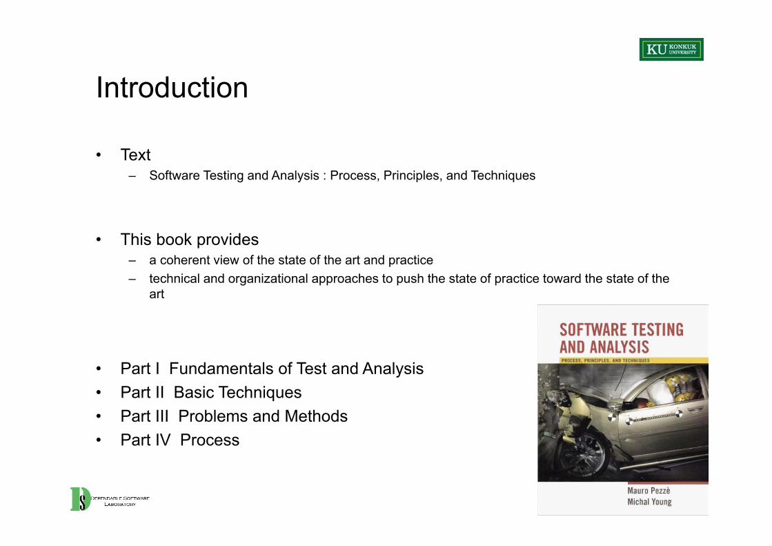
Introduction

• Text– Software Testing and Analysis : Process, Principles, and Techniques

• This book provides– a coherent view of the state of the art and practice– technical and organizational approaches to push the state of practice toward the state of the

art

• Part I Fundamentals of Test and Analysis• Part II Basic Techniques• Part III Problems and Methods• Part IV Process

2

Part I. Fundamentals of Test and Analysis

Chapter 1. Software Test and Analysis in a Nutshell

Learning Objectives

• View the “big picture'' of software quality in the context of a software development project and organization

• Introduce the range of software verification and validation activities

• Provide a rationale for selecting and combining them within a software development process

5

Engineering Processes

• All engineering processes have two common activities– Construction activities– Checking activities

• In software engineering (purpose: construction of high quality software)– Construction activities– Verification activities

• We are focusing on software verification activities.

6

Software Verification Activities

• Software verification activities take various forms– for non-critical products for mass markets– for highly-customized products– for critical products

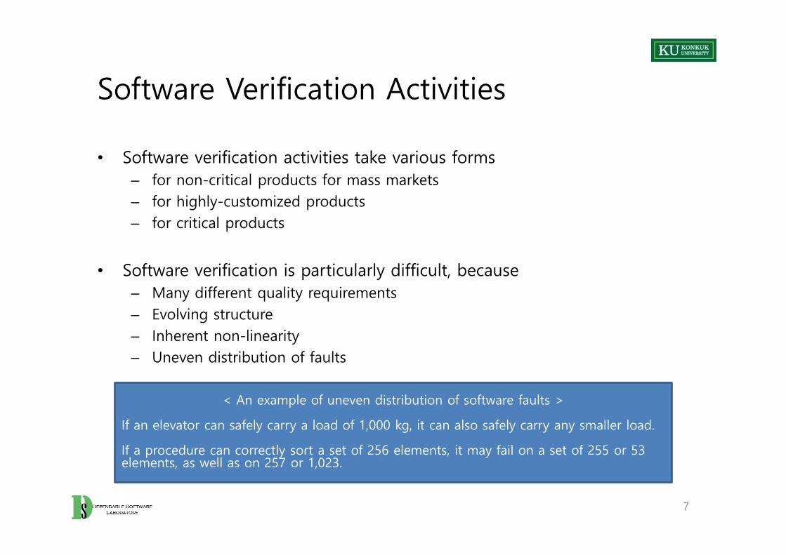
• Software verification is particularly difficult, because– Many different quality requirements – Evolving structure– Inherent non-linearity– Uneven distribution of faults

7

< An example of uneven distribution of software faults >

If an elevator can safely carry a load of 1,000 kg, it can also safely carry any smaller load.

If a procedure can correctly sort a set of 256 elements, it may fail on a set of 255 or 53 elements, as well as on 257 or 1,023.

Variety of Approaches

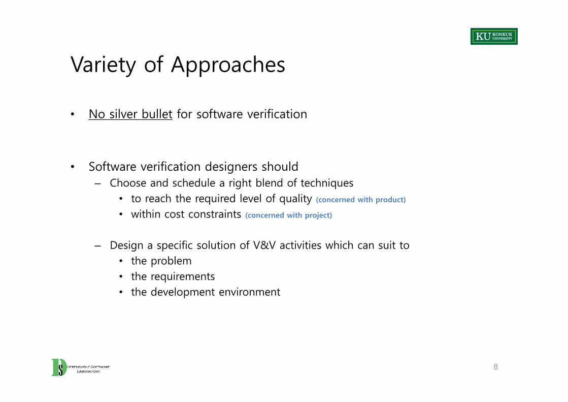
• No silver bullet for software verification

• Software verification designers should– Choose and schedule a right blend of techniques

• to reach the required level of quality (concerned with product)

• within cost constraints (concerned with project)

– Design a specific solution of V&V activities which can suit to • the problem• the requirements• the development environment

8

Basic Questions

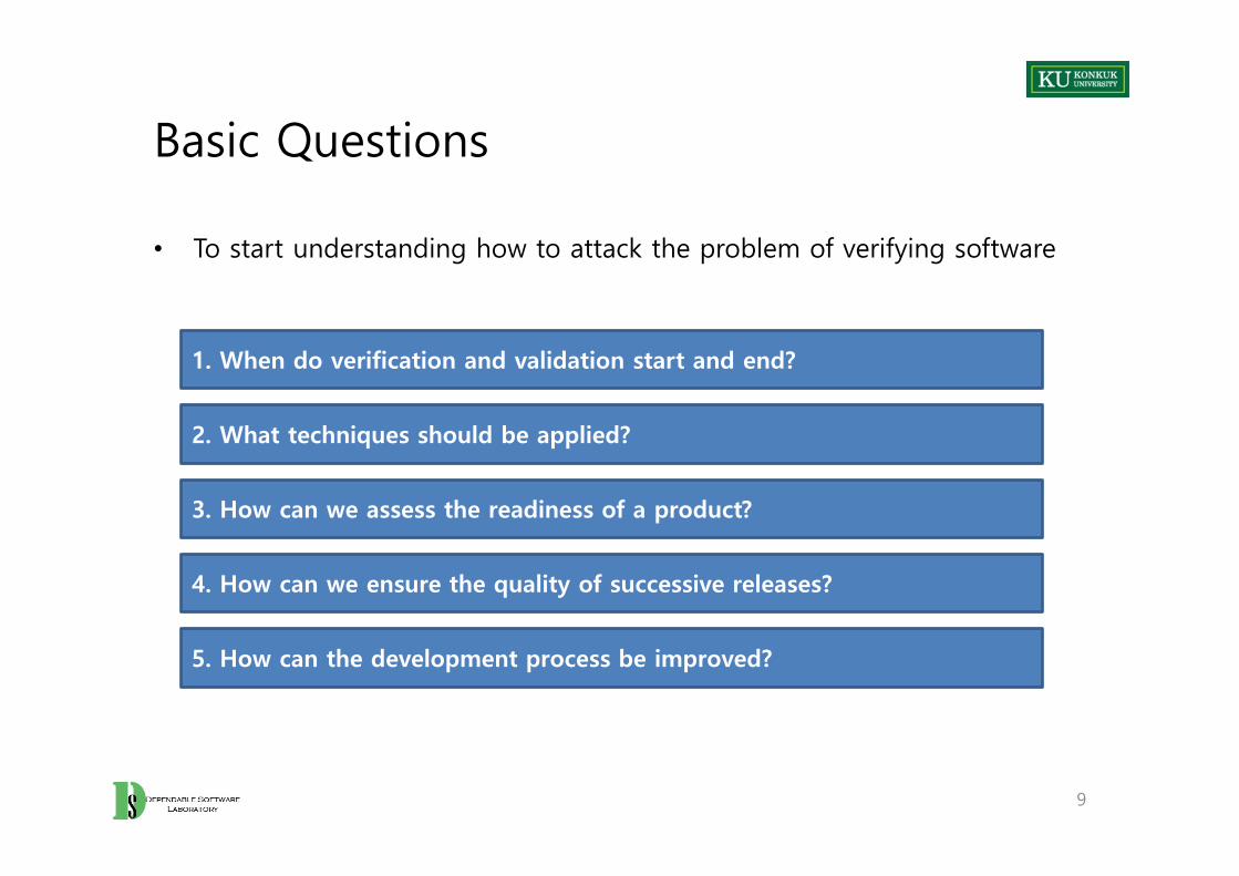
• To start understanding how to attack the problem of verifying software

9

1. When do verification and validation start and end?

2. What techniques should be applied?

3. How can we assess the readiness of a product?

4. How can we ensure the quality of successive releases?

5. How can the development process be improved?

1. When Do Verification and Validation Start and End?

• Test – A widely used V&V activity– Usually known as a last activity in software development process– But, not the test activity is “test execution”– Test execution is a small part of V&V process

• V&V start as soon as we decide to build a software product, or even before.

• V&V last far beyond the product delivery as long as the software is in use, to cope with evolution and adaptations to new conditions.

10

Early Start: From Feasibility Study

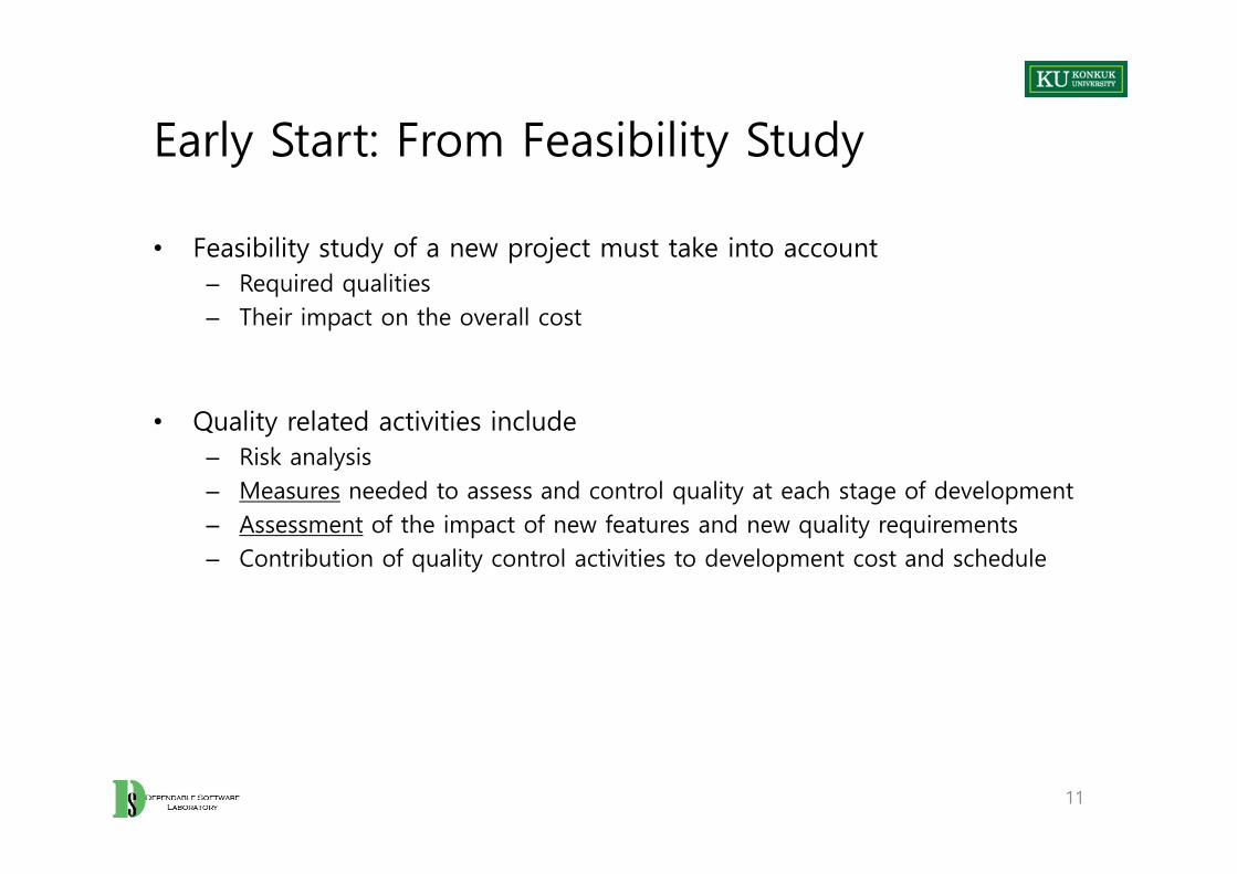
• Feasibility study of a new project must take into account – Required qualities – Their impact on the overall cost

• Quality related activities include– Risk analysis – Measures needed to assess and control quality at each stage of development – Assessment of the impact of new features and new quality requirements– Contribution of quality control activities to development cost and schedule

11

Long Lasting: Beyond Maintenance

• Maintenance activities include– Analysis of changes and extensions– Generation of new test suites for the added functionalities– Re-executions of tests to check for non regression of software functionalities

after changes and extensions– Fault tracking and analysis

12

2. What Techniques Should Be Applied?

• No single A&T technique can serve all purposes.

• The primary reasons for combining techniques are:– Effectiveness for different classes of faults

( analysis instead of testing for race conditions )– Applicability at different points in a project

( inspection for early requirements validation )– Differences in purpose

( statistical testing to measure reliability )– Tradeoffs in cost and assurance

( expensive technique for key properties )

13

14

RequirementsElicitation

RequirementsSpecification

ArchitecturalDesign

DetailedDesign Unit Coding Integration &

Delivery Maintenance

Plan

ning

& m

onit

orin

gVe

rifi

cati

on o

f sp

ecs

test

cas

e ex

ecut

ion

and

sw v

alid

atio

n

Identify qualites

Plan acceptance test

Validate specifications

Plan system test

Plan unit & integration test

Gen

erat

ion

of t

ests

Inspect architectural design

Analyze architectural design

Inspect detailed design

Monitor the A&T process

Generate system test

Generate integration test

Generate unit test

Generate regression test

Update regression test

Code inspection

Design scaffolding

Design oracles

Execute unit test

Execute integration test

Analyze coverage

Generate structural test

Execute system test

Execute acceptance test

Execute regression test

Collect data on faults

analyze faults and improve the processProc

ess

impr

ovem

ent

3. How Can We Assess the Readiness of a Product?

• A&T activities aim at revealing faults during development.– We cannot reveal or remove all faults.– A&T cannot last infinitely.

• We have to know whether products meet the quality requirements or not.– We must specify the required level of dependability. Measurement

– We can determine when that level has been attained. Assessment

15

4. How Can We Ensure the Quality of Successive Releases? • A&T activities does not stop at the first release.

• Software products operate for many years, and undergo many changes.– To adapt to environment changes– To serve new and changing user requirements

• Quality tasks after delivery include– Test and analysis of new and modified code– Re-execution of system tests– Extensive record-keeping

16

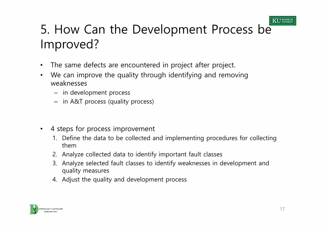
5. How Can the Development Process be Improved?

• The same defects are encountered in project after project.• We can improve the quality through identifying and removing

weaknesses – in development process– in A&T process (quality process)

• 4 steps for process improvement1. Define the data to be collected and implementing procedures for collecting

them2. Analyze collected data to identify important fault classes3. Analyze selected fault classes to identify weaknesses in development and

quality measures 4. Adjust the quality and development process

17

Summary

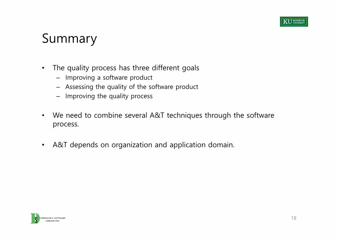
• The quality process has three different goals– Improving a software product– Assessing the quality of the software product– Improving the quality process

• We need to combine several A&T techniques through the software process.

• A&T depends on organization and application domain.

18

19

Chapter 2. A Framework for Testing and Analysis

Learning Objectives

• Introduce dimensions and tradeoff between test and analysis activities

• Distinguish validation from verification activities

• Understand limitations and possibilities of test and analysis activities

21

Verification and Validation

• Validation: “Does the software system meets the user's real needs?”– Are we building the right software?

• Verification: “Does the software system meets the requirements specifications?”– Are we building the software right?

ActualRequirements

SWSpecs

System

Validation Verification

22

V&V Depends on the Specification

• Unverifiable (but validatable) specification: “If a user presses a request button at floor i, an available elevator must arrive at floor i soon.“

• Verifiable specification: “If a user presses a request button at floor i, an available elevator must arrive at floor i within 30 seconds“

23

1 2 3 4 5 6 7 8

V-Model of V&V Activities

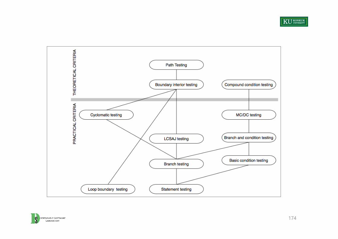
24

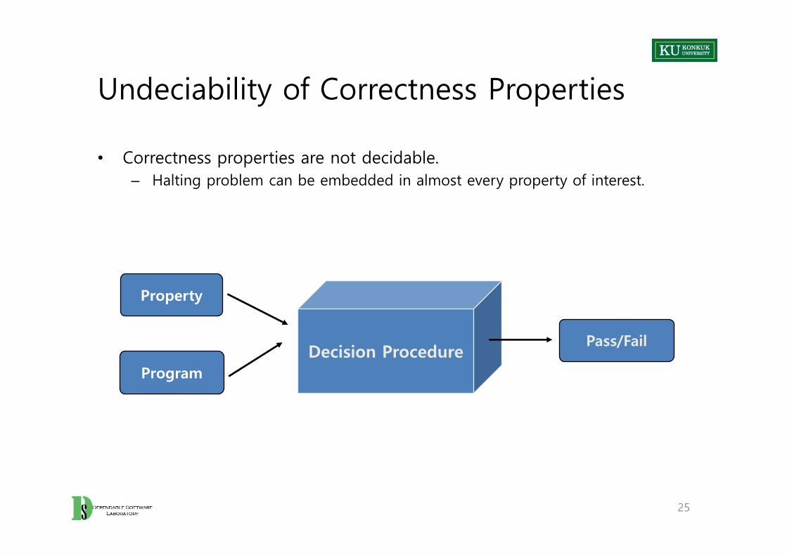
Undeciability of Correctness Properties

• Correctness properties are not decidable.– Halting problem can be embedded in almost every property of interest.

25

Decision Procedure

Property

Program

Pass/Fail

Verification Trade-off Dimensions

• Optimistic inaccuracy– We may accept some programs

that do not possess the property.– It may not detect all violations. – Example: Testing

• Pessimistic inaccuracy– It is not guaranteed to accept a

program even if the program does possess the property being analyzed, because of false alarms.

– Example: Automated program analysis

• Simplified properties– It reduces the degree of freedom

by simplifying the property to check.

– Example: Model Checking

26

Perfect verification ofarbitrary properties bylogical proof or exhaustivetesting (Infinite effort)

Model checking:Decidable but possiblyintractable checking of

simple temporalproperties.

Theorem proving:Unbounded effort to

verify generalproperties.

Precise analysis ofsimple syntacticproperties.

Typical testingtechniques

Data flowanalysis

Optimisticinaccuracy

Pessimisticinaccuracy

Simplifiedproperties

Terms related to Pessimistic and Optimistic

27

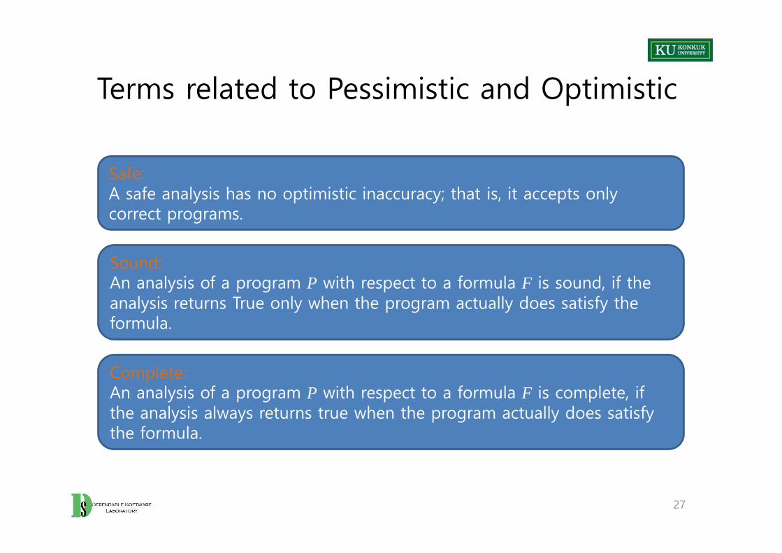
Safe:A safe analysis has no optimistic inaccuracy; that is, it accepts only correct programs.

Sound:An analysis of a program P with respect to a formula F is sound, if the analysis returns True only when the program actually does satisfy the formula.

Complete:An analysis of a program P with respect to a formula F is complete, if the analysis always returns true when the program actually does satisfy the formula.

Summary

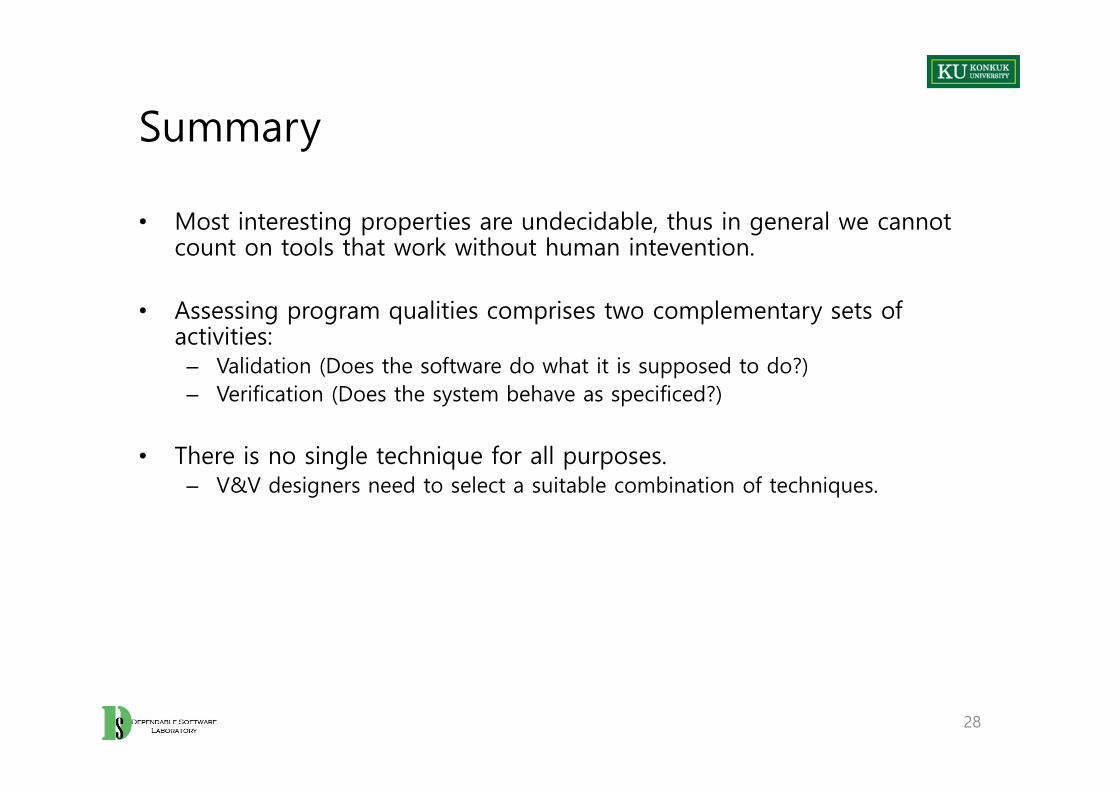
• Most interesting properties are undecidable, thus in general we cannot count on tools that work without human intevention.

• Assessing program qualities comprises two complementary sets of activities:

– Validation (Does the software do what it is supposed to do?)– Verification (Does the system behave as specificed?)

• There is no single technique for all purposes.– V&V designers need to select a suitable combination of techniques.

28

29

Chapter 3. Basic Principles

Learning Objectives

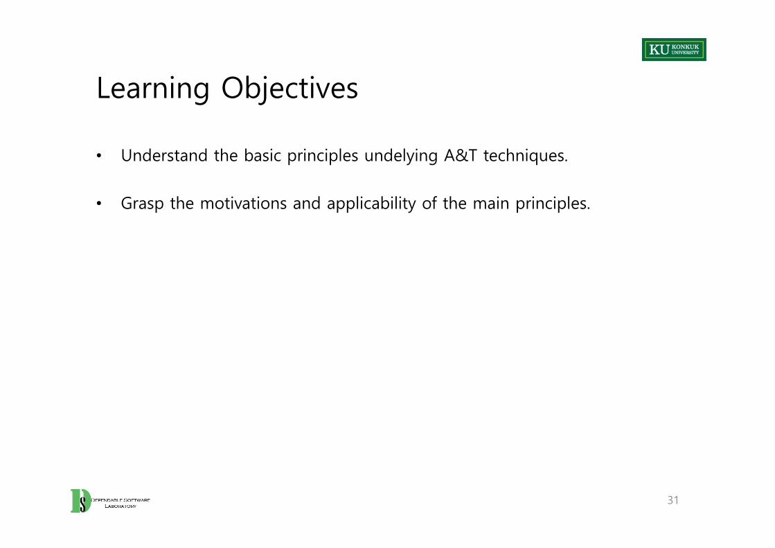
• Understand the basic principles undelying A&T techniques.

• Grasp the motivations and applicability of the main principles.

31

Main A&T Principles

• Principles for general engineering:– Partition: divide and conquer– Visibility: making information accessible– Feedback: tuning the development process

• Principles specific to software A&T:– Sensitivity: better to fail every time than sometimes– Redundancy: making intentions explicit– Restriction: making the problem easier

32

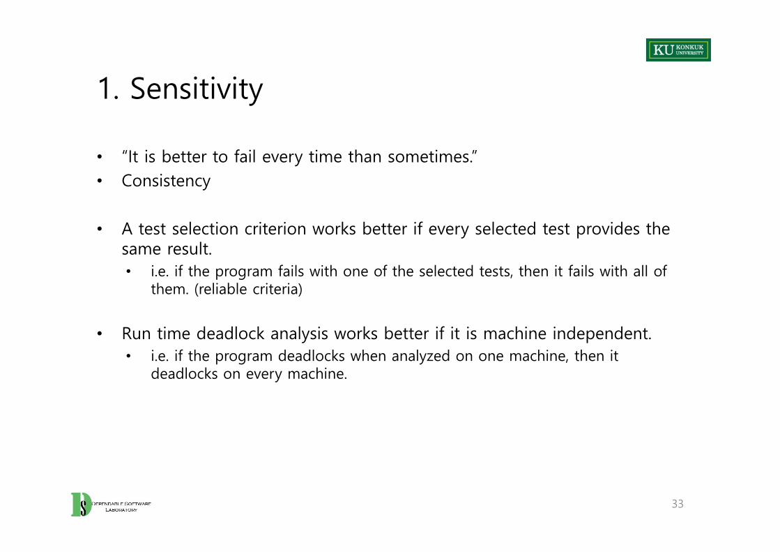
1. Sensitivity

• “It is better to fail every time than sometimes.”• Consistency

• A test selection criterion works better if every selected test provides the same result.• i.e. if the program fails with one of the selected tests, then it fails with all of

them. (reliable criteria)

• Run time deadlock analysis works better if it is machine independent.• i.e. if the program deadlocks when analyzed on one machine, then it

deadlocks on every machine.

33

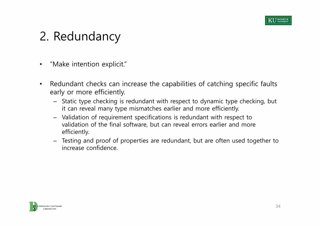
2. Redundancy

• “Make intention explicit.”

• Redundant checks can increase the capabilities of catching specific faults early or more efficiently.

– Static type checking is redundant with respect to dynamic type checking, but it can reveal many type mismatches earlier and more efficiently.

– Validation of requirement specifications is redundant with respect to validation of the final software, but can reveal errors earlier and more efficiently.

– Testing and proof of properties are redundant, but are often used together to increase confidence.

34

3. Restriction

• “Make the problem easier.”

• Suitable restrictions can reduce hard (unsolvable) problems to simpler (solvable) problems.

• A weaker spec may be easier to check: – It is impossible (in general) to show that pointers are used correctly, but the

simple Java requirement that pointers are initialized before use is simple to enforce.

• A stronger spec may be easier to check: – It is impossible (in general) to show that type errors do not occur at run-time

in a dynamically typed language, but statically typed languages impose stronger restrictions that are easily checkable.

35

4. Partition

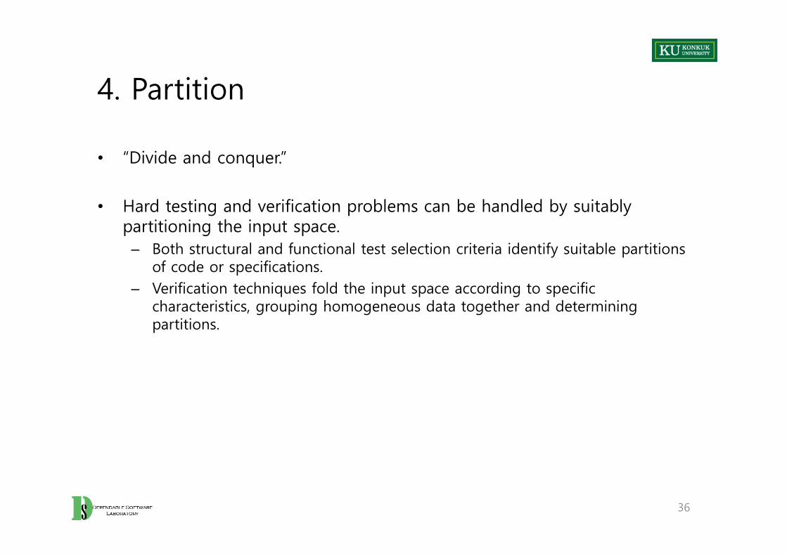
• “Divide and conquer.”

• Hard testing and verification problems can be handled by suitably partitioning the input space.

– Both structural and functional test selection criteria identify suitable partitions of code or specifications.

– Verification techniques fold the input space according to specific characteristics, grouping homogeneous data together and determining partitions.

36

5. Visibility

• “Make information accessible.”

• The ability to measure progress or status against goals– X visibility = ability to judge how we are doing on X– schedule visibility = “Are we ahead or behind schedule?” – quality visibility = “Does quality meet our objectives?”

• Involves setting goals that can be assessed at each stage of development.

• The biggest challenge is early assessment– Assessing specifications and design with respect to product quality

37

6. Feedback

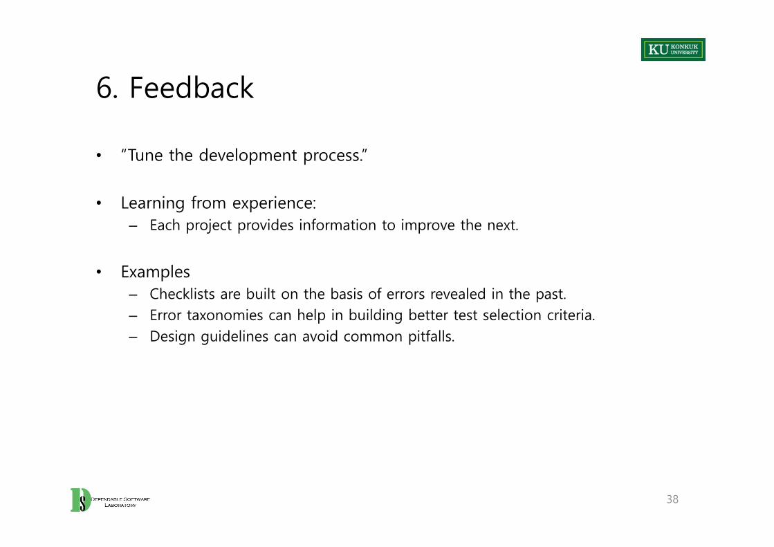
• “Tune the development process.”

• Learning from experience: – Each project provides information to improve the next.

• Examples– Checklists are built on the basis of errors revealed in the past.– Error taxonomies can help in building better test selection criteria.– Design guidelines can avoid common pitfalls.

38

Summary

• The discipline of A&T is characterized by 6 main principles:– Sensitivity: better to fail every time than sometimes– Redundancy: making intentions explicit– Restriction: making the problem easier– Partition: divide and conquer– Visibility: making information accessible– Feedback: tuning the development process

• They can be used to understand advantages and limits of different approaches and compare different techniques.

39

40

Chapter 4. Test and Analysis Activities within a

Software Process

Learning Objectives

• Understand the role of quality in the development process

• Build an overall picture of the quality process

• Identify the main characteristics of a quality process– Visibility– Anticipation of activities– Feedback

42

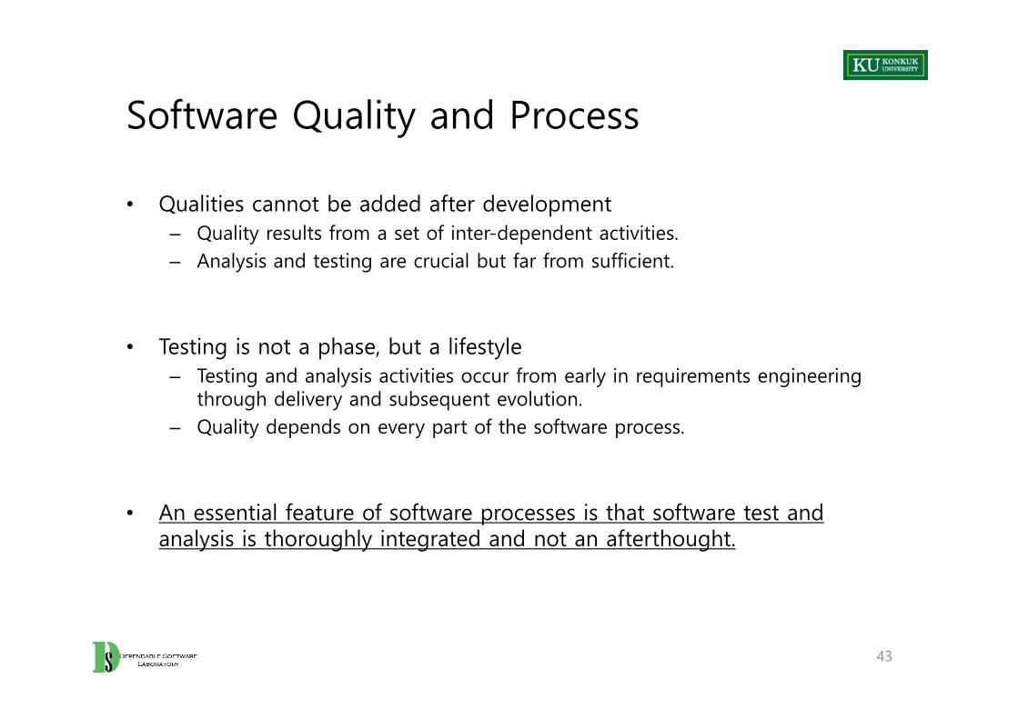
Software Quality and Process

• Qualities cannot be added after development– Quality results from a set of inter-dependent activities.– Analysis and testing are crucial but far from sufficient.

• Testing is not a phase, but a lifestyle– Testing and analysis activities occur from early in requirements engineering

through delivery and subsequent evolution. – Quality depends on every part of the software process.

• An essential feature of software processes is that software test and analysis is thoroughly integrated and not an afterthought.

43

Quality Process

• Quality process– A set of activities and responsibilities

• Focused on ensuring adequate dependability • Concerned with project schedule or with product usability

• Quality process provides a framework for – Selecting and arranging A&T activities – Considering interactions and trade-offs with other important goals

44

An Example of Other Important Goals

• “High dependability” vs. “Time to market”

• Mass market products: – Better to achieve a reasonably high degree of dependability on a tight

schedule than to achieve ultra-high dependability on a much longer schedule

• Critical medical devices:– Better to achieve ultra-high dependability on a much longer schedule than a

reasonably high degree of dependability on a tight schedule

45

Planning and Monitoring

• Quality process – A&T planning– Balances several activities across the whole development process– Selects and arranges them to be as cost-effective as possible– Improves early visibility

• A&T planning is integral to the quality process.– Quality goals can be achieved only through careful planning.

46

Process Visibility

• A process is visible to the extent that one can answer the question:– How does our progress compare to our plan?– Example: Are we on schedule? How far ahead or behind?

• The quality process can achieve adequate visibility, if one can gain strong confidence in the quality of the software system, before it reaches final testing

– Quality activities are usually placed as early as possible• Design test cases at the earliest opportunity• Uses analysis techniques on software artifacts produced before actual

code – Motivates the use of “proxy” measures

• Example: the number of faults in design or code is not a true measure of reliability, but we may count faults discovered in design inspections as an early indicator of potential quality problems.

47

A&T Plan

• A comprehensive description of the quality process that includes:– objectives and scope of A&T activities– documents and other items that must be available – items to be tested– features to be tested and not to be tested– analysis and test activities – staff involved in A&T– constraints– pass and fail criteria– schedule– deliverables– hardware and software requirements– risks and contingencies

48

Quality Goals

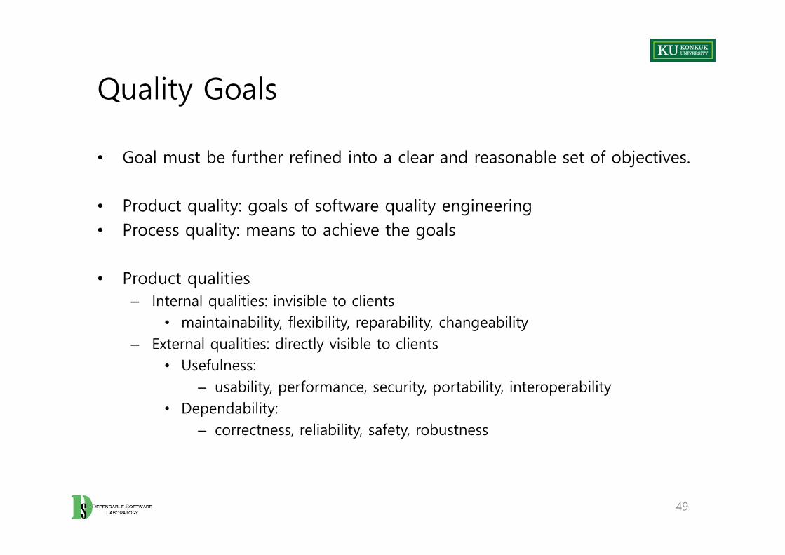
• Goal must be further refined into a clear and reasonable set of objectives.

• Product quality: goals of software quality engineering• Process quality: means to achieve the goals

• Product qualities– Internal qualities: invisible to clients

• maintainability, flexibility, reparability, changeability– External qualities: directly visible to clients

• Usefulness:– usability, performance, security, portability, interoperability

• Dependability:– correctness, reliability, safety, robustness

49

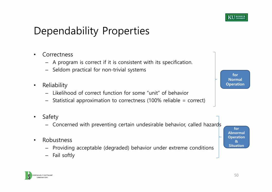
Dependability Properties

• Correctness– A program is correct if it is consistent with its specification.– Seldom practical for non-trivial systems

• Reliability– Likelihood of correct function for some ”unit” of behavior– Statistical approximation to correctness (100% reliable = correct)

• Safety– Concerned with preventing certain undesirable behavior, called hazards

• Robustness– Providing acceptable (degraded) behavior under extreme conditions– Fail softly

50

for Normal

Operation

for Abnormal Operation

&Situation

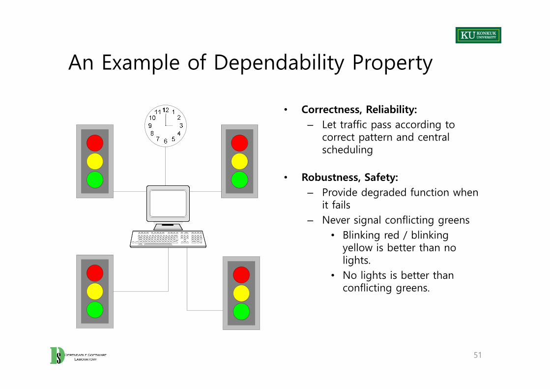
An Example of Dependability Property

• Correctness, Reliability: – Let traffic pass according to

correct pattern and central scheduling

• Robustness, Safety: – Provide degraded function when

it fails– Never signal conflicting greens

• Blinking red / blinking yellow is better than no lights.

• No lights is better than conflicting greens.

51

Relationship among Dependability Properties

52

Reliable Correct Safe Robust

Robust but not Safe:Catastrophic failures can occur

Safe but not Correct: Annoying failures can occur

Correct but not Safe nor Robust: The specification is inadequate

Reliable but not Correct: Failures can occur rarely

Analysis

• Do not involve actual execution of program source code– Manual inspection– Automated static analysis

• Inspection technique– Can be applied to essentially any document – Takes a considerable amount of time – Re-inspecting a changed component can be expensive.

• Automatic static analysis– Can be applied to some formal representations of requirements models– Not to natural language documents– Substituting machine cycles for human effort makes them particularly cost-

effective.

53

Testing

• Executed late in development, but• Start as early as possible

• Early test generation has several advantages:– Tests are generated independently from code, when the specifications are

fresh in the mind of analysts.– Generation of test cases may highlight inconsistencies and incompleteness of

the corresponding specifications.

– Tests may be used as compendium of the specifications by the programmers.

54

Improving the Process

• Long lasting errors are common.• It is important to structure the process for

– Identifying the most critical persistent faults– Tracking them to frequent errors– Adjusting the development and quality processes to eliminate errors

• Feedback mechanisms are the main ingredient of the quality process for identifying and removing errors.

55

Organizational Factors

• Different teams for development and quality?– Separate development and quality teams is common in large organizations.

• Different roles for development and quality?– Test designer is a specific role in many organizations– Mobility of people and roles by rotating engineers over development and

testing tasks among different projects is a possible option.

56

An Example of Allocation of Responsibility

• Allocating tasks and responsibilities is a complex job

• Unit testing – to the development team (requires detailed knowledge of the code)– but the quality team may control the results (structural coverage)

• Integration, system and acceptance testing – to the quality team– but the development team may produce scaffolding and oracles

• Inspection and walk-through – to mixed teams

• Regression testing– to quality and maintenance teams

• Process improvement related activities – to external specialists interacting with all teams

57

Ch 4, slide 58

Summary

• A&Ts are complex activties that must be sutiably planned and monitored.

• A good quality process obeys some basic principles:– Visibility– Early activities– Feedback

• Aims at– Reducing occurrences of faults– Assessing the product dependability before delivery– Improving the process

59

Part II. Basic Techniques

Chapter 5. Finite Models

Learning Objectives

• Understand goals and implications of finite state abstraction

• Learn how to model program control flow with graphs

• Learn how to model the software system structure with call graphs

• Learn how to model finite state behavior with finite state machines

62

Model

• A model is– A representation that is simpler than the artifact it represents,– But preserves some important attributes of the actual artifact

• Our concern is with models of program execution.

63

Directed Graph

• Directed graph:– N : set of nodes– E : set of edges (relation on the set of nodes)

64

a

b c

b a c

N = { a, b, c }E = { (a, b), (a, c), (c, a) }

Directed Graph with Labels

• We can label nodes with the names or descriptions of the entities they represent.

– If nodes a and b represent program regions containing assignment statements, we might draw the two nodes and an edge (a, b) connecting them in this way:

65

x = y + z;

a = f(x);

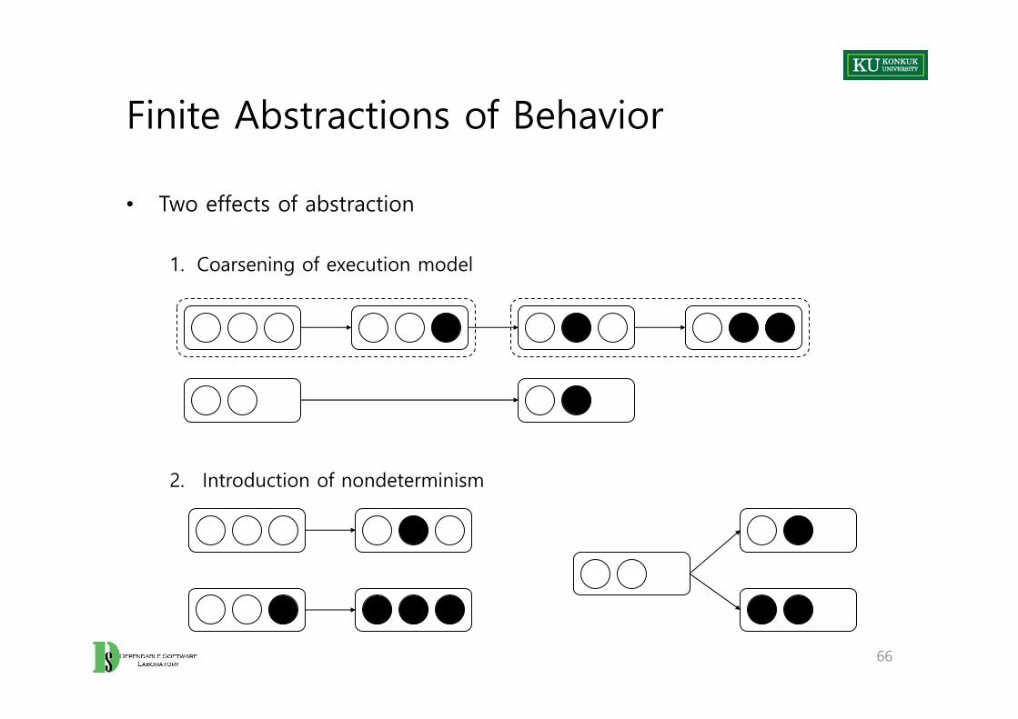
Finite Abstractions of Behavior

• Two effects of abstraction

1. Coarsening of execution model

2. Introduction of nondeterminism

66

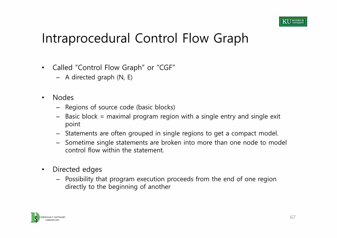
Intraprocedural Control Flow Graph

• Called “Control Flow Graph” or “CGF”– A directed graph (N, E)

• Nodes – Regions of source code (basic blocks)– Basic block = maximal program region with a single entry and single exit

point– Statements are often grouped in single regions to get a compact model.– Sometime single statements are broken into more than one node to model

control flow within the statement.

• Directed edges – Possibility that program execution proceeds from the end of one region

directly to the beginning of another

67

An Example of CFG

public static String collapseNewlines(String argStr){

char last = argStr.charAt(0);StringBuffer argBuf = new StringBuffer();

for (int cIdx = 0 ; cIdx < argStr.length(); cIdx++){

char ch = argStr.charAt(cIdx);if (ch != '\n' || last != '\n'){

argBuf.append(ch);last = ch;

}}

return argBuf.toString();}

68

{char last = argStr.charAt(0);StringBuffer argBuf = new StringBuffer();

for (int cIdx = 0 ;

{char ch = argStr.charAt(cIdx);if (ch != '\n'

cIdx < argStr.length();

True

True

{argBuf.append(ch);last = ch;

}

True

}cIdx++)

return argBuf.toString();}

False

False

|| last != '\n')

public static String collapseNewlines(String argStr)

False

b2

b4

b3

b5

b6

b7

b8

The Use of CFG

• CFG may be used directly to define thoroughness criteria for testing.– Chapter 9. Test Case Selection and Adequacy– Chapter 12. Structural Testing

• Often, CFG is used to define another model which is used to define a thoroughness criterion

– Example: LCSAJ is derived from the CGF• Essential sub-paths of the CFG from one branch to another

69

LCSAJ (Linear Code Sequence And Jump)

70

{char last = argStr.charAt(0);StringBuffer argBuf = new StringBuffer();

for (int cIdx = 0 ;

{char ch = argStr.charAt(cIdx);if (ch != '\n'

cIdx < argStr.length();

True

True

{argBuf.append(ch);last = ch;

}

True

}cIdx++)

return argBuf.toString();}

False

False

|| last != '\n')

public static String collapseNewlines(String argStr)

False

b2

b4

b3

b5

b6

b7

b8

b1

jX

jT

jE

jL

From Sequence of Basic Blocks To

entry b1 b2 b3 jX

entry b1 b2 b3 b4 jT

entry b1 b2 b3 b4 b5 jE

entry b1 b2 b3 b4 b5 b6 b7 jL

jX b8 Return

jL b3 b4 jT

jL b3 b4 b5 jE

jL b3 b4 b5 b6 b7 jL

Call Graphs

• “Interprocedural Control Flow Graph”– A directed graph (N, E)

• Nodes– Represent procedures, methods, functions, etc.

• Edges– Represent ‘call’ relation

• Call graph presents many more design issues and trade-off than CFG.– Overestimation of call relation– Context sensitive/insensitive

71

Overestimation in a Call Graph

• The static call graph includes calls through dynamic bindings that never occur in execution.

72

public class C{public static CcFactory(Stringkind){

if (kind=="C")return new C();if (kind=="S")return new S();return null;

}void foo(){

System.out.println("Youcalledtheparent'smethod");}public static void main(Stringargs[]){

(new A()).check();}

}class Sextends C{void foo(){

System.out.println("Youcalledthechild'smethod");}

}class A{void check(){

CmyC =C.cFactory("S");myC.foo();

}}

A.check()

C.foo() S.foo() CcFactory(string)

never occur in execution

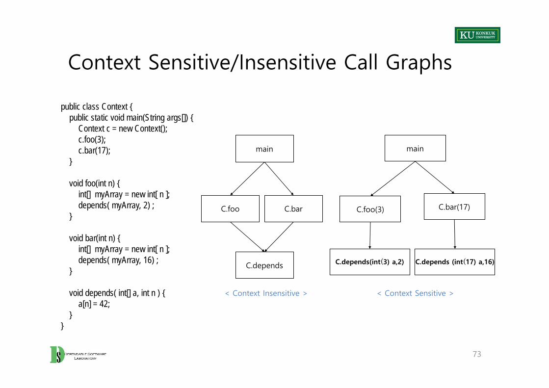
Context Sensitive/Insensitive Call Graphs

73

public class Context {public static void main(String args[]) {

Context c = new Context(); c.foo(3); c.bar(17);

}

void foo(int n) {int[] myArray = new int[ n ]; depends( myArray, 2) ;

}

void bar(int n) {int[] myArray = new int[ n ]; depends( myArray, 16) ;

}

void depends( int[] a, int n ) {a[n] = 42;

}}

main

C.foo C.bar

C.depends

main

C.foo(3) C.bar(17)

C.depends(int(3) a,2) C.depends (int(17) a,16)

< Context Insensitive > < Context Sensitive >

Calling Paths in Context Sensitive Call Graphs

74

A

B

D

F

H

C

E

G

I

J

1 context A

2 contexts AB AC

4 contexts ABD ABE ACD ACE

8 contexts …

16 calling contexts … exponentially grow.

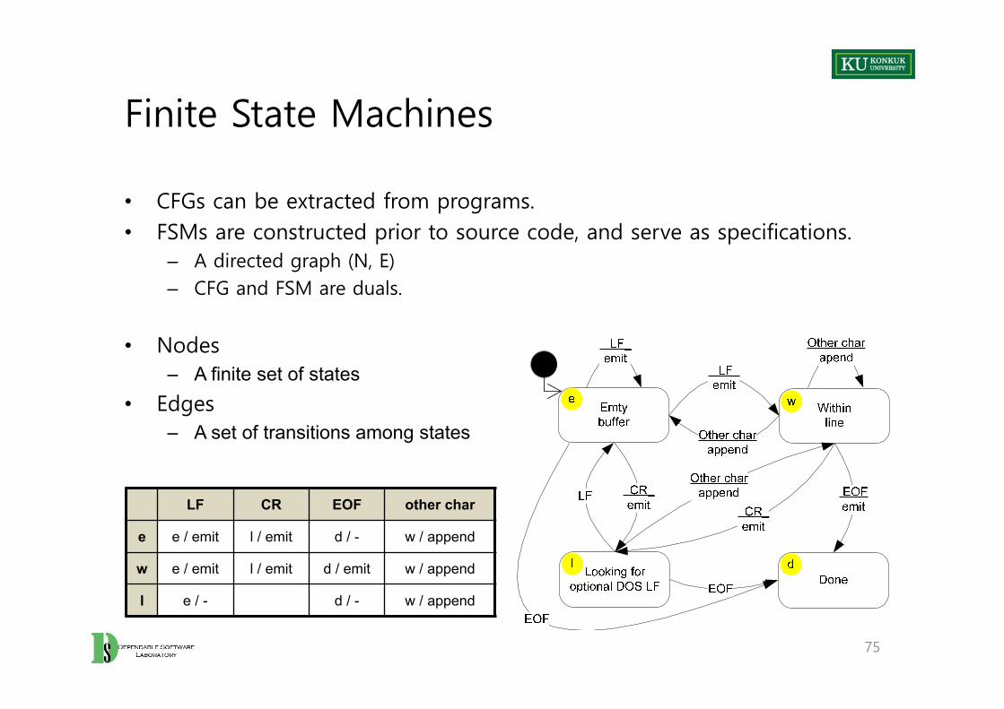
Finite State Machines

• CFGs can be extracted from programs.• FSMs are constructed prior to source code, and serve as specifications.

– A directed graph (N, E)– CFG and FSM are duals.

• Nodes– A finite set of states

• Edges– A set of transitions among states

75

LF CR EOF other char

e e / emit l / emit d / - w / append

w e / emit l / emit d / emit w / append

l e / - d / - w / append

Correctness Relations for FSM Models

76

Abstract Function for Modeling FSMs

77

Modeling with abstraction

Summary

• Models must be much simpler than the artifact they describe in order to be understandable and analyzable.

• Models must be sufficiently detailed to be useful.

• CFG are built from software program.

• FSM can be built before software program to documente behavior.

78

79

Chapter 6. Data Dependency and Data Flow Models

Learning Objectives

• Understand basics of data-flow models and the related concepts (def-use pairs, dominators…)

• Understand some analyses that can be performed with the data-flow model of a program

– Data flow analyses to build models– Analyses that use the data flow models

• Understand basic trade-offs in modeling data flow

81

Why Data Flow Models Need?

• Models from Chapter 5 emphasized control flow only.– Control flow graph, call graph, finite state machine

• We also need to reason about data dependence.– To reason about transmission of information through program variables– “Where does this value of x come from?”– “What would be affected by changing this? “

• Many program analyses and test design techniques use data flow information and dependences

– Often in combination with control flow

82

Definition-Use Pairs

• A def-use (du) pair associates a point in a program where a value is produced with a point where it is used

• Definition: where a variable gets a value– Variable declaration– Variable initialization– Assignment– Values received by a parameter

• Use: extraction of a value from a variable– Expressions– Conditional statements– Parameter passing– Returns

83

Def-Use Pairs

84

...if (...) {

x = ... ; ... }y = ... + x + ... ;…

x = ...

if (...) {

...

y = ... + x + ...

...

...

Definition: x gets a value

Use: the value of x is extractedDef-Use

path

Def-Use Pairs

85

/** Euclid's algorithm */

public int gcd(int x, int y) {int tmp; // A: def x, y, tmp while (y != 0) { // B: use y

tmp = x % y; // C: def tmp; use x, yx = y; // D: def x; use yy = tmp; // E: def y; use tmp

}return x; // F: use x

}

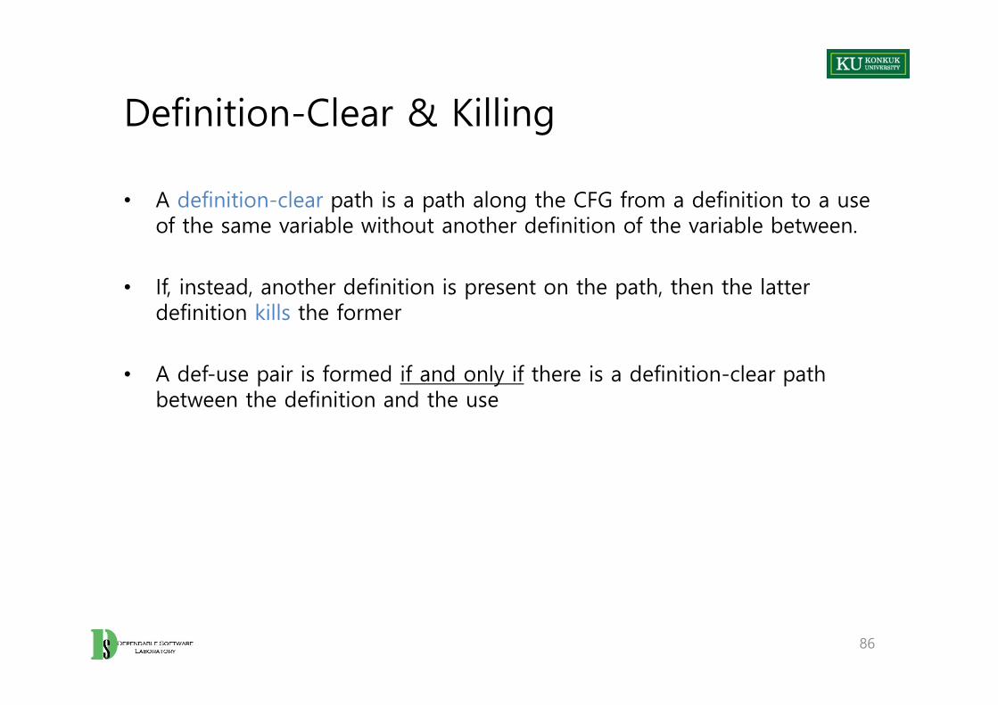
Definition-Clear & Killing

• A definition-clear path is a path along the CFG from a definition to a use of the same variable without another definition of the variable between.

• If, instead, another definition is present on the path, then the latter definition kills the former

• A def-use pair is formed if and only if there is a definition-clear path between the definition and the use

86

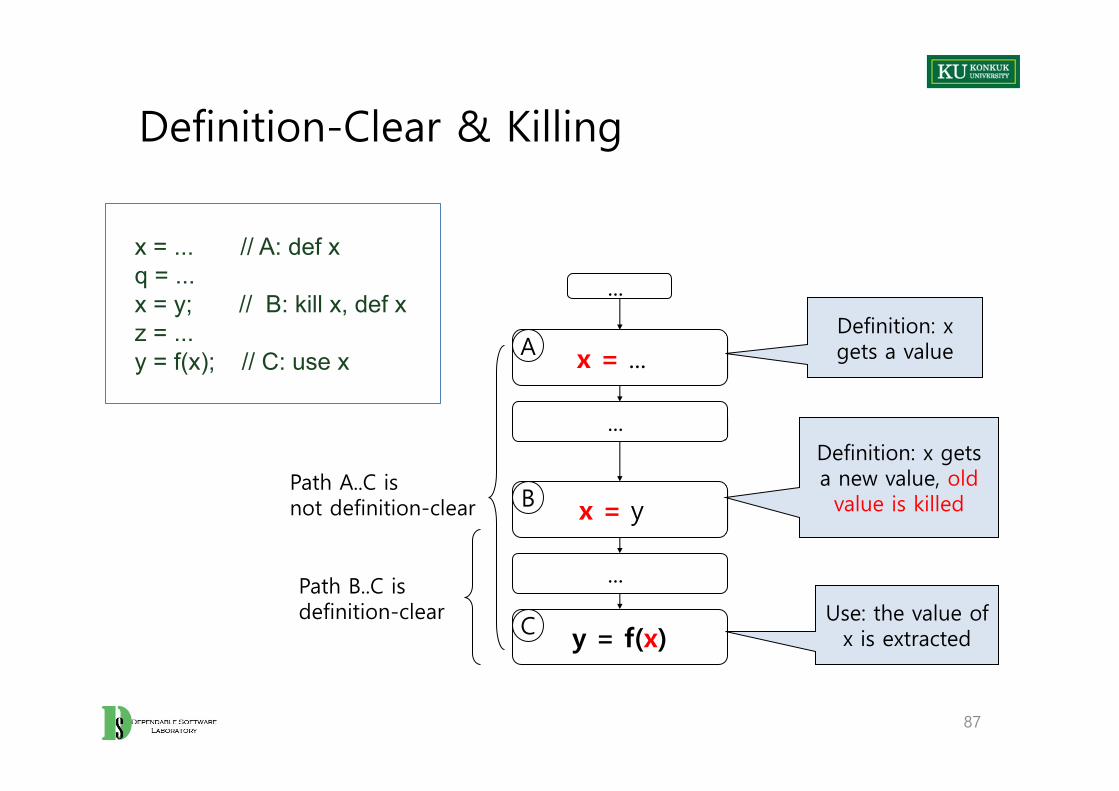
Definition-Clear & Killing

87

x = ... // A: def xq = ... x = y; // B: kill x, def xz = ... y = f(x); // C: use x x = ...

...

...

Definition: x gets a value

Use: the value of x is extracted

A

x = y

Definition: x gets a new value, old value is killed

...

y = f(x)

B

C

Path B..C is definition-clear

Path A..C is not definition-clear

(Direct) Data Dependence Graph

• Direct data dependence graph– A direct graph (N, E)

• Nodes: as in the control flow graph (CFG)• Edges: def-use (du) pairs, labelled with the variable name

88

x

/** Euclid's algorithm */

public int gcd(int x, int y) {int tmp; // A: def x, y, tmp while (y != 0) { // B: use y

tmp = x % y; // C: def tmp; use x, yx = y; // D: def x; use yy = tmp; // E: def y; use tmp

}return x; // F: use x

}

Control Dependence

• Data dependence– “Where did these values come from?”

• Control dependence – “Which statement controls whether this statement executes?”– A directed graph

• Nodes: as in the CFG• Edges: unlabelled, from entry/branching points to controlled blocks

89

/** Euclid's algorithm */

public int gcd(int x, int y) {int tmp; // A: def x, y, tmp while (y != 0) { // B: use y

tmp = x % y; // C: def tmp; use x, yx = y; // D: def x; use yy = tmp; // E: def y; use tmp

}return x; // F: use x

}

Dominator

• Pre-dominators in a rooted, directed graph can be used to make this intuitive notion of “controlling decision” precise.

• Node M dominates node N, if every path from the root to N passes through M.

– A node will typically have many dominators, but except for the root, there is a unique immediate dominator of node N which is closest to N on any path from the root, and which is in turn dominated by all the other dominators of N.

– Because each node (except the root) has a unique immediate dominator, the immediate dominator relation forms a tree.

• Post-dominators are calculated in the reverse of the control flow graph, using a special “exit” node as the root.

90

An Example of Dominators

• A pre-dominates all nodes.• G post-dominates all nodes.

• F and G post-dominate E.• G is the immediate post-

dominator of B.

• C does not post-dominate B.

• B is the immediate pre-dominator of G.

• F does not pre-dominate G.

91

A

B

C

D

E

F

G

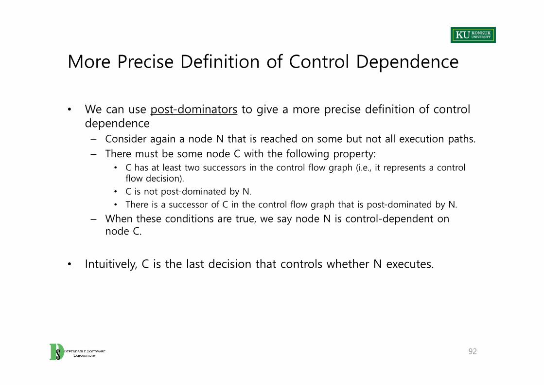
More Precise Definition of Control Dependence

• We can use post-dominators to give a more precise definition of control dependence

– Consider again a node N that is reached on some but not all execution paths.– There must be some node C with the following property:

• C has at least two successors in the control flow graph (i.e., it represents a control flow decision).

• C is not post-dominated by N.• There is a successor of C in the control flow graph that is post-dominated by N.

– When these conditions are true, we say node N is control-dependent on node C.

• Intuitively, C is the last decision that controls whether N executes.

92

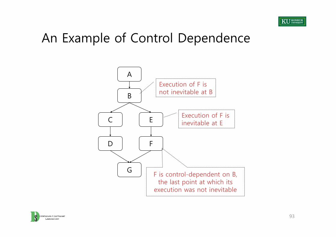
An Example of Control Dependence

93

A

B

C

D

E

F

GF is control-dependent on B,

the last point at which itsexecution was not inevitable

Execution of F is not inevitable at B

Execution of F is inevitable at E

Data Flow Analysis

• Describes the algorithms used to compute data flow information. – Basic algorithms used widely in compilers, test and analysis tools, and other

software tools.

• Too difficult Skipped.

94

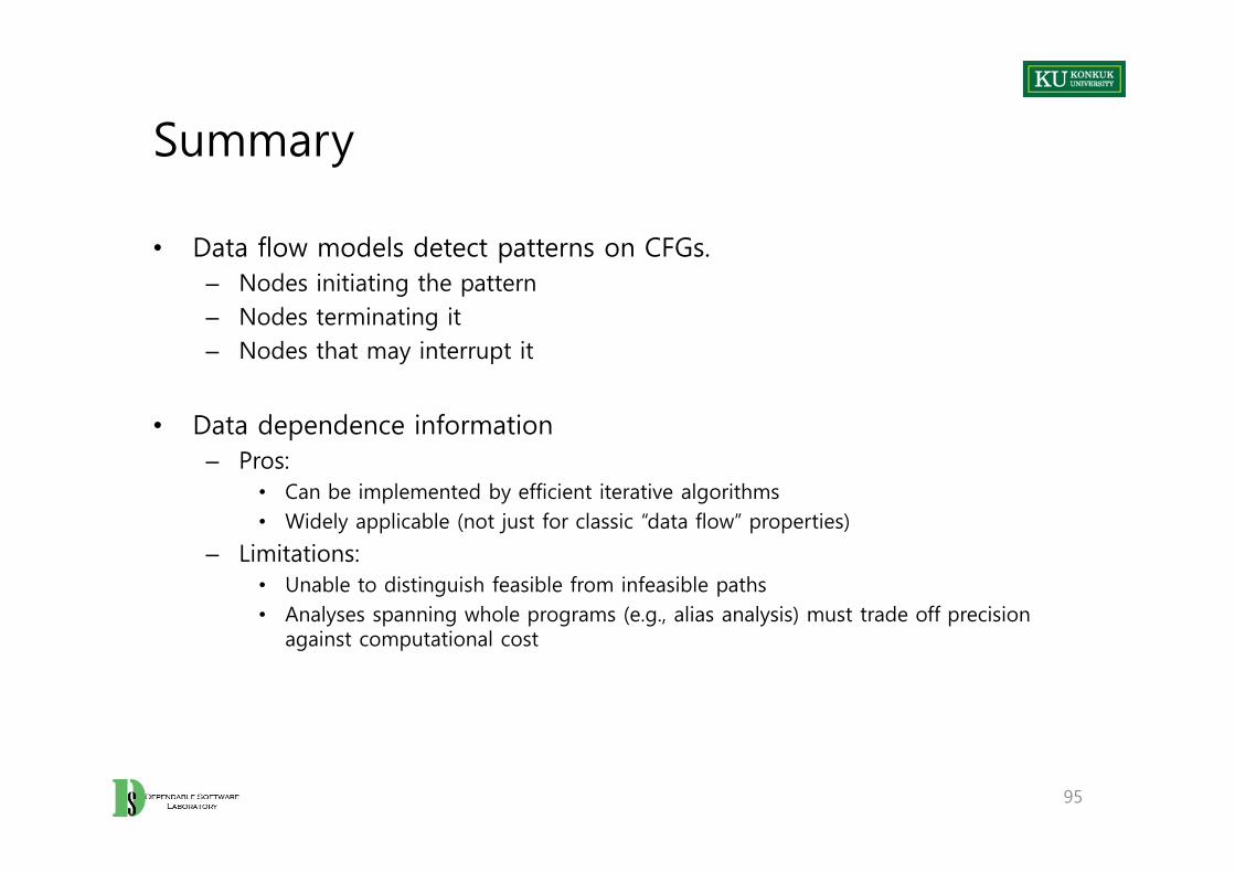
Summary

• Data flow models detect patterns on CFGs.– Nodes initiating the pattern– Nodes terminating it– Nodes that may interrupt it

• Data dependence information– Pros:

• Can be implemented by efficient iterative algorithms• Widely applicable (not just for classic “data flow” properties)

– Limitations:• Unable to distinguish feasible from infeasible paths• Analyses spanning whole programs (e.g., alias analysis) must trade off precision

against computational cost

95

96

Chapter 7. Symbolic Execution and Proof of Properties

Learning Objectives

• Understand the goal and implication of symbolically executing programs

• Learn how to use assertions to summarize infinite executions• Learn how to reason about program correctness• Learn how to use symbolic execution to reason about program

properties

• Understand limits and problems of symbolic execution

98

Symbolic Execution

• Builds predicates that characterize – Conditions for executing paths – Effects of the execution on program state

• Bridges program behavior to logic

• Finds important applications in – Program analysis– Test data generation– Formal verification (proofs) of program correctness

• Rigorous proofs of properties of critical subsystems– Example: safety kernel of a medical device

• Formal verification of critical properties particularly resistant to dynamic testing – Example: security properties

• Formal verification of algorithm descriptions and logical designs– less complex than implementations

99

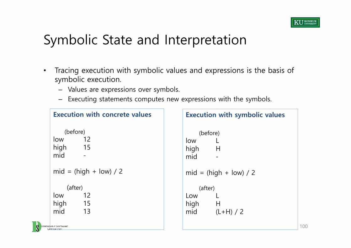
Symbolic State and Interpretation

• Tracing execution with symbolic values and expressions is the basis of symbolic execution.

– Values are expressions over symbols.– Executing statements computes new expressions with the symbols.

100

Execution with concrete values

(before)low 12high 15mid -

mid = (high + low) / 2

(after)low 12high 15mid 13

Execution with symbolic values

(before)low Lhigh Hmid -

mid = (high + low) / 2

(after)Low Lhigh Hmid (L+H) / 2

Tracing Execution with Symbolic Executions

101

char *binarySearch( char *key, char *dictKeys[ ], char *dictValues[ ], int dictSize) {

int low = 0; int high = dictSize - 1; int mid; int comparison;

while (high >= low) {mid = (high + low) / 2; comparison = strcmp( dictKeys[mid], key );if (comparison < 0) {

low = mid + 1;} else if ( comparison > 0 ) {

high = mid - 1;} else {

return dictValues[mid];}

}return 0;

}

Execution with symbolic values

(before)low = 0

∧ high = (H-1)/2 -1∧ mid = (H-1)/2

while (high >= low) {

(after)low = 0

∧ high = (H-1)/2 -1∧ mid = (H-1)/2∧ (H-1)/2 - 1 >= 0... ∧ not((H-1)/2 - 1 >= 0)

when true

when false

∧ ∀k, 0 ≤ k < size : dictKeys[k] = key → L ≤ k ≤ H∧ H ≥ M ≥ L

supposed

Summary Information

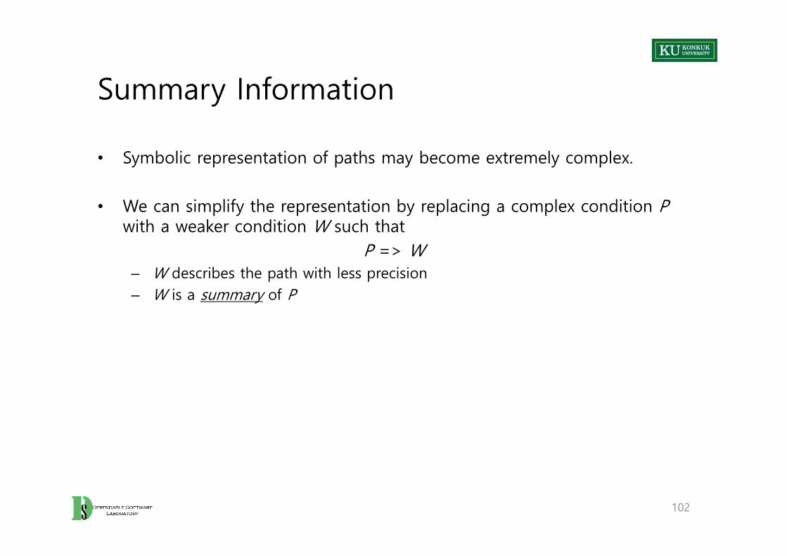
• Symbolic representation of paths may become extremely complex.

• We can simplify the representation by replacing a complex condition Pwith a weaker condition W such that

P => W– W describes the path with less precision– W is a summary of P

102

An Example of Summary Information

• If we are reasoning about the correctness of the binary search algorithm, – In “ mid = (high+low)/2 “

• The weaker condition contains less information, but still enough to reason about correctness.

103

Weaker condition:

low = L∧ high = H∧ mid = M∧ L <= M <= H

Complete condition:

low = L∧ high = H∧ mid = M∧ M = (L+H) / 2

Weaker Precondition

• The weaker predicate L <= mid <= H is chosen based on what must be true for the program to execute correctly.

– It cannot be derived automatically from source code.– It depends on our understanding of the code and our rationale for believing

it to be correct.

• A predicate stating what should be true at a given point can be expressed in the form of an assertion

• Weakening the predicate has a cost for testing– Satisfying the predicate is no longer sufficient to find data that forces

program execution along that path. • Test data satisfying a weaker predicate W is necessary to execute the

path, but it may not be sufficient.• Showing that W cannot be satisfied shows path infeasibility.

104

Loops and Assertions

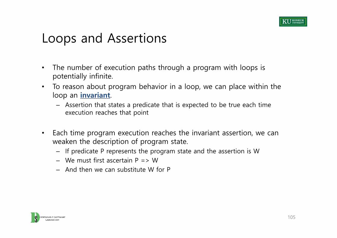
• The number of execution paths through a program with loops is potentially infinite.

• To reason about program behavior in a loop, we can place within the loop an invariant.

– Assertion that states a predicate that is expected to be true each time execution reaches that point

• Each time program execution reaches the invariant assertion, we can weaken the description of program state.

– If predicate P represents the program state and the assertion is W– We must first ascertain P => W – And then we can substitute W for P

105

Precondition and Postcondition

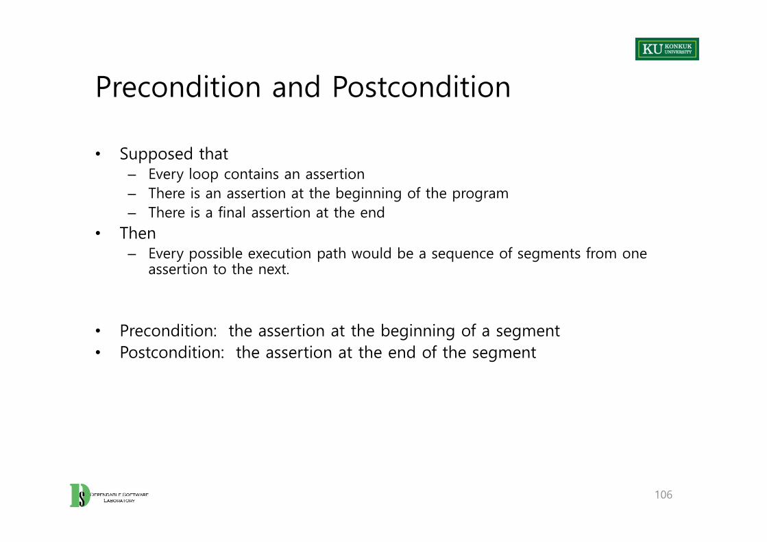
• Supposed that– Every loop contains an assertion– There is an assertion at the beginning of the program– There is a final assertion at the end

• Then– Every possible execution path would be a sequence of segments from one

assertion to the next.

• Precondition: the assertion at the beginning of a segment• Postcondition: the assertion at the end of the segment

106

Verification of Program Correctness

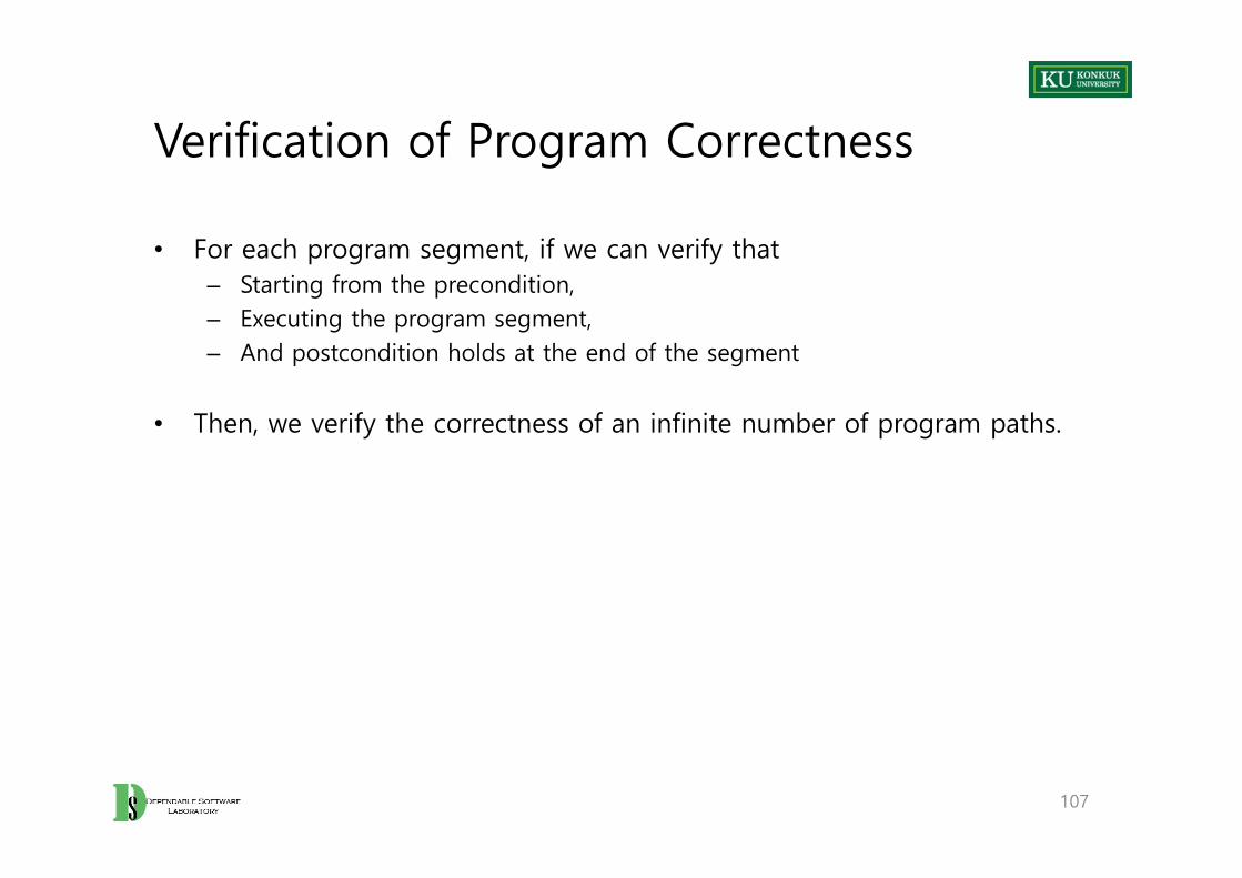
• For each program segment, if we can verify that – Starting from the precondition,– Executing the program segment,– And postcondition holds at the end of the segment

• Then, we verify the correctness of an infinite number of program paths.

107

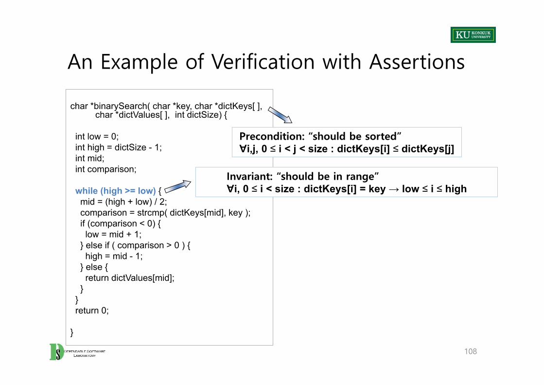
An Example of Verification with Assertions

108

char *binarySearch( char *key, char *dictKeys[ ], char *dictValues[ ], int dictSize) {

int low = 0; int high = dictSize - 1; int mid; int comparison;

while (high >= low) {mid = (high + low) / 2; comparison = strcmp( dictKeys[mid], key );if (comparison < 0) {

low = mid + 1;} else if ( comparison > 0 ) {

high = mid - 1;} else {

return dictValues[mid];}

}return 0;

}

Precondition: “should be sorted”∀i,j, 0 ≤ i < j < size : dictKeys[i] ≤ dictKeys[j]

Invariant: “should be in range”∀i, 0 ≤ i < size : dictKeys[i] = key → low ≤ i ≤ high

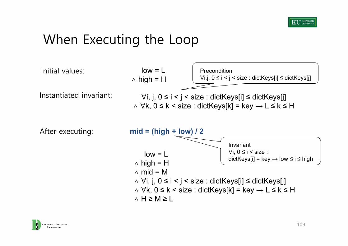
When Executing the Loop

109

low = L∧ high = H

∀i, j, 0 ≤ i < j < size : dictKeys[i] ≤ dictKeys[j]∧ ∀k, 0 ≤ k < size : dictKeys[k] = key → L ≤ k ≤ H

Initial values:

Instantiated invariant:

low = L∧ high = H ∧ mid = M∧ ∀i, j, 0 ≤ i < j < size : dictKeys[i] ≤ dictKeys[j]∧ ∀k, 0 ≤ k < size : dictKeys[k] = key → L ≤ k ≤ H∧ H ≥ M ≥ L

After executing: mid = (high + low) / 2Invariant∀i, 0 ≤ i < size : dictKeys[i] = key → low ≤ i ≤ high

Precondition∀i,j, 0 ≤ i < j < size : dictKeys[i] ≤ dictKeys[j]

After executing the Loop

110

low = M+1∧ high = H ∧ mid = M∧ ∀i, j, 0 ≤ i < j < size : dictKeys[i] ≤ dictKeys[j]∧ ∀k, 0 ≤ k < size : dictKeys[k] = key → L ≤ k ≤ H∧ H ≥ M ≥ L∧ dictkeys[M] < key

After executing the loop :

The new instance of the invariant:

∀i, j, 0 ≤ i < j < size : dictKeys[i] ≤ dictKeys[j]∧ ∀k, 0 ≤ k < size : dictKeys[k] = key → M+1 ≤ k <= H

If the invariant is satisfied, the loop is correct woth respect to the preconditions and the invariant.

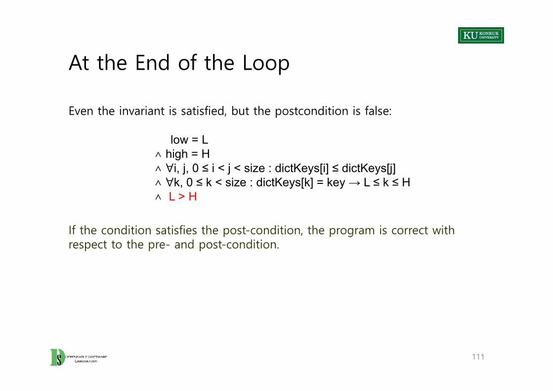
At the End of the Loop

Even the invariant is satisfied, but the postcondition is false:

If the condition satisfies the post-condition, the program is correct with respect to the pre- and post-condition.

111

low = L∧ high = H ∧ ∀i, j, 0 ≤ i < j < size : dictKeys[i] ≤ dictKeys[j]∧ ∀k, 0 ≤ k < size : dictKeys[k] = key → L ≤ k ≤ H∧ L > H

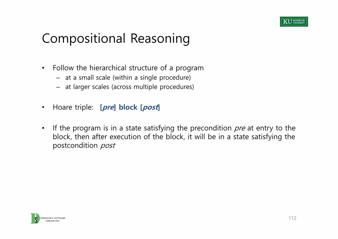
Compositional Reasoning

• Follow the hierarchical structure of a program– at a small scale (within a single procedure) – at larger scales (across multiple procedures)

• Hoare triple: [pre] block [post]

• If the program is in a state satisfying the precondition pre at entry to the block, then after execution of the block, it will be in a state satisfying the postcondition post

112

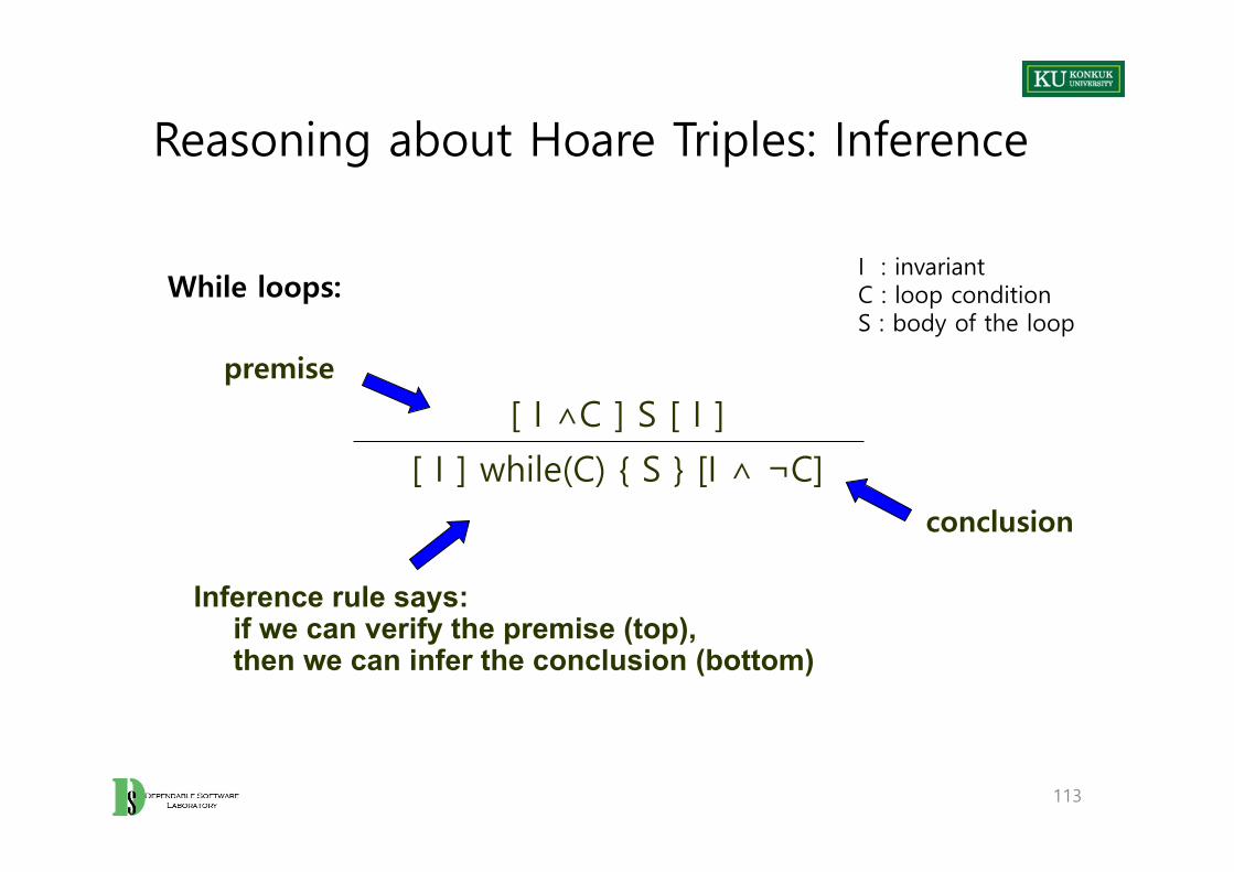
Reasoning about Hoare Triples: Inference

113

[ I ∧C ] S [ I ]

[ I ] while(C) { S } [I ∧ ¬C]

Inference rule says:if we can verify the premise (top), then we can infer the conclusion (bottom)

premise

conclusion

While loops:I : invariantC : loop conditionS : body of the loop

Other Inference Rule

114

if statement:

[P ∧ C] thenpart [Q] [P ∧ ¬C] elsepart [Q][P] if (C) {thenpart} else {elsepart} [Q]

Reasoning Style

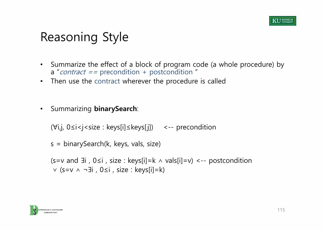
• Summarize the effect of a block of program code (a whole procedure) by a “contract == precondition + postcondition “

• Then use the contract wherever the procedure is called

• Summarizing binarySearch:

(∀i,j, 0≤i<j<size : keys[i]≤keys[ j]) <-- precondition

s = binarySearch(k, keys, vals, size)

(s=v and ∃i , 0≤i , size : keys[i]=k ∧ vals[i]=v) <-- postcondition∨ (s=v ∧ ¬∃i , 0≤i , size : keys[i]=k)

115

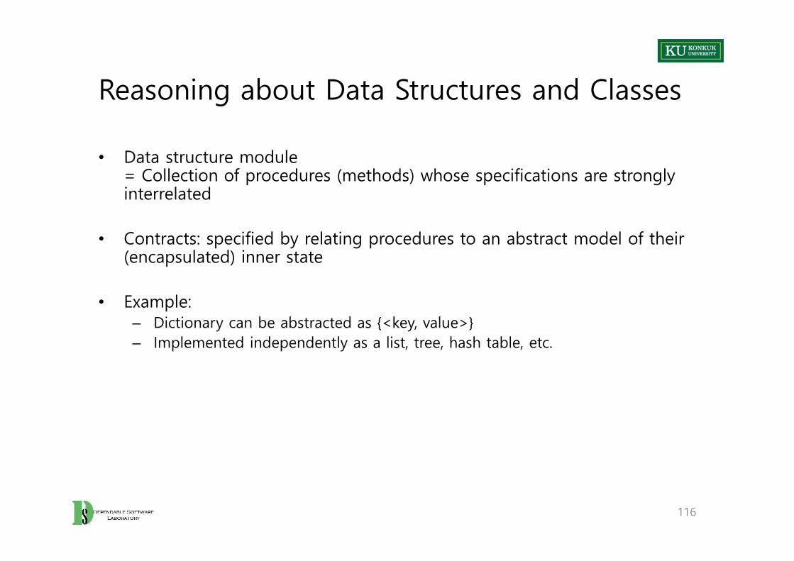
Reasoning about Data Structures and Classes

• Data structure module = Collection of procedures (methods) whose specifications are strongly interrelated

• Contracts: specified by relating procedures to an abstract model of their (encapsulated) inner state

• Example: – Dictionary can be abstracted as {<key, value>}– Implemented independently as a list, tree, hash table, etc.

116

Structural Invariant & Abstract Function

• Structural invariants are the structural characteristics that must be maintained. (directly analogous to loop invariants)

– Example: Each method in a search tree class should maintain the ordering of keys in the tree.

• Abstract function maps concrete objects to abstract model states.– Example: Dictionary

• [<k,v> ∈ Φ(dict) ]• o = dict.get(k)• [ o = v ]

117

Summary

• Symbolic execution is a bridge from an operational view of program execution to logical and mathematical statements.

• Basic symbolic execution technique is the execution using symbols.

• Symbolic execution for loops, procedure calls, and data structures: proceed hierarchically

– compose facts about small parts into facts about larger parts

• Fundamental technique for– Generating test data– Verifying systems – Performing or checking program transformations

• Tools are essential to scale up.

118

119

Chapter 8. Finite State Verification

Learning Objectives

• Understand the purpose and appropriate uses of finite-state verification– Understand how FSV mitigates weaknesses of testing– Understand how testing complements FSV

• Understand modeling for FSV as a balance between cost and precision

• Distinguish explicit state enumeration from analysis of implicit models– Understand why implicit models are sometimes (but not always) more

effective

121

Overview

• Most important properties of program execution are not decidable.– Finite state verification can automatically prove some significant properties of

a finite model of the infinite execution space.

• Need to balance trade-offs among – Generality of properties to be checked– Class of programs or models that can be checked– Computational effort in checking– Human effort in producing models and specifying properties

122

Resources and Results

123

Properties to be proved

Computational costhigh

complex

low

simple

controland data flow

models

and formal reasoningsymbolic execution

and formal reasoning

finite stateverification

Applies techniques from symbolic execution and formal verification to models that abstract the potentially infinite state space of program behavior into finite representations

Cost of FSV

• Human effort and skill are required. – to prepare a finite state model – to prepare a suitable specification for automated analysis

• Iterative process of FSV1. Prepare a model and specify properties2. Attempt verification 3. Receive reports of impossible or unimportant faults4. Refine the specification or the model

124

Finite State Verification Framework

125

Applications for Finite State Verifications

• Concurrent (multi-threaded, distributed, ...) system– Difficult to test thoroughly (apparent non-determinism based on scheduler)– Sensitive to differences between development environment and field

environment– First and most well-developed application of FSV

• Data models– Difficult to identify “corner cases” and interactions among constraints, or to

thoroughly test them

• Security– Some threats depend on unusual (and untested) use

126

An Example: Modeling Concurrent System

• Deriving a good finite state model is hard.

• Example: FSM model of a program with multiple threads of control– Simplifying assumptions

• We can determine in advance the number of threads.• We can obtain a finite state machine model of each thread.• We can identify the points at which processes can interact.

– State of the whole system model • Tuple of states of individual process models

– Transition • Transition of one or more of the individual processes, acting individually or in

concert

127

State Space Explosion – An Example

• On-line purchasing system

• Specification– In-memory data structure initialized by reading configuration tables at system

start-up– Initialization of the data structure must appear atomic. – The system must be reinitialized on occasion.– The structure is kept in memory.

• Implementation (with bugs)

– No monitor (e.g. Java synchronized), because it’s too expensive.– But, use double-checked locking idiom* for a fast system

*Bad decision, broken idiom ... but extremely hard to find the bug through testing.

128

On-line Purchasing System - Implementation

129

class Table1 {

private static Table1 ref = null; private boolean needsInit = true; private ElementClass [ ] theValues;private Table1() { }

public static Table1 getTable1() {if (ref == null)

{ synchedInitialize(); }return ref;

}

private static synchronized void synchedInitialize() {if (ref == null) {

ref = new Table1(); ref.initialize();

} }

public void reinit() { needsInit = true; }

private synchronized void initialize() {. . . needsInit = false;

}

public int lookup(int i) {if (needsInit) {

synchronized(this) {if (needsInit) {

this.initialize();}

}}return theValues[i].getX() + theValues[i].getY();

}

. . .}

Analysis on On-line Purchasing System

• Start from models of individual threads

– Systematically trace all the possible interleaving of threads

– Like hand-executing all possible sequences of execution, but automated

• Analysis begins by constructing an FSM model of each individual thread.

130

(a)lookup()

needsInit==true

(b)

obtain lock

(c)

(f)reading

needsInit==false

(e)

(d)modifyingneedsInit==false

needsInit==true

needsInit=false

release lock

E

(x)reinit()

needsInit=true

(y)

E

Analysis (Continued)

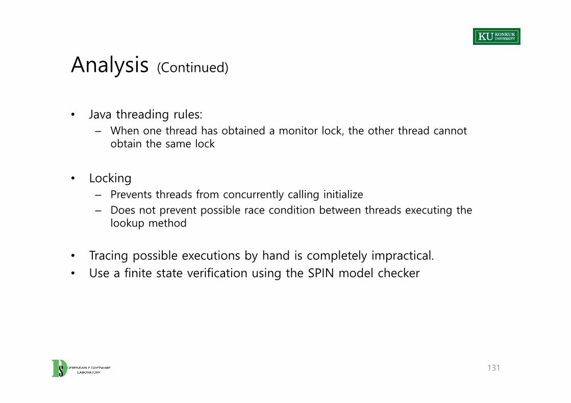
• Java threading rules:– When one thread has obtained a monitor lock, the other thread cannot

obtain the same lock

• Locking – Prevents threads from concurrently calling initialize– Does not prevent possible race condition between threads executing the

lookup method

• Tracing possible executions by hand is completely impractical.• Use a finite state verification using the SPIN model checker

131

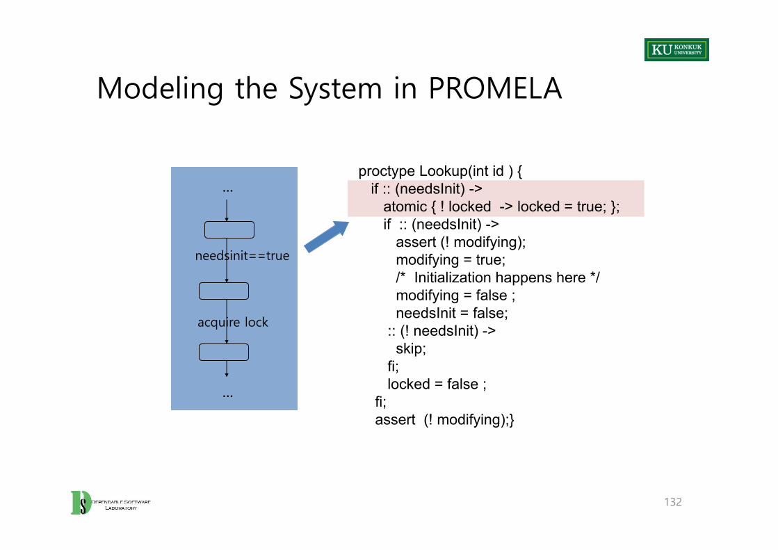
Modeling the System in PROMELA

132

needsinit==true

acquire lock

...

...proctype Lookup(int id ) {

if :: (needsInit) -> atomic { ! locked -> locked = true; };if :: (needsInit) ->

assert (! modifying); modifying = true; /* Initialization happens here */modifying = false ; needsInit = false;

:: (! needsInit) -> skip;

fi;locked = false ;

fi;assert (! modifying);}

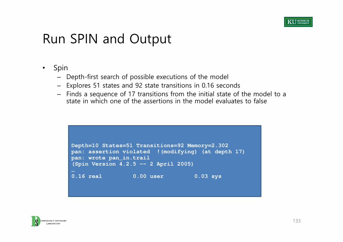
Run SPIN and Output

• Spin– Depth-first search of possible executions of the model– Explores 51 states and 92 state transitions in 0.16 seconds – Finds a sequence of 17 transitions from the initial state of the model to a

state in which one of the assertions in the model evaluates to false

133

Depth=10 States=51 Transitions=92 Memory=2.302 pan: assertion violated !(modifying) (at depth 17)pan: wrote pan_in.trail(Spin Version 4.2.5 -- 2 April 2005)…0.16 real 0.00 user 0.03 sys

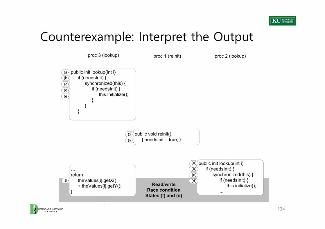
Counterexample: Interpret the Output

134

Read/writeRace condition

States (f) and (d)

…return

theValues[i].getX()+ theValues[i].getY();

}

proc 3 (lookup)

public void reinit(){ needsInit = true; }

(x)

proc 1 (reinit)

public init lookup(int i)if (needsInit) {

synchronized(this) {if (needsInit) {

this.initialize();}

}}

(y)

proc 2 (lookup)

(a)(b)(c)(d)(e)

(f)

public init lookup(int i)if (needsInit) {

synchronized(this) {if (needsInit) {

this.initialize();...

(a)(b)(c)(d)

The State Space Explosion Problem

• Dining philosophers - looking for deadlock with SPIN

5 phils+forks 145 statesdeadlock found

10 phils+forks 18,313 stateserror trace too long to be useful

15 phils+forks 148,897 stateserror trace too long to be useful

• Team Practice and Homework!!!– From 2017

135

The Model Correspondence Problem

• Verifying correspondence between model and program– Extract the model from the source code with verified procedures

• Blindly mirroring all details state space explosion • Omitting crucial detail “false alarm” reports

– Produce the source code automatically from the model• Most applicable within well-understood domains

– Conformance testing• Combination of FSV and testing is a good tradeoff

136

Granularity of Modeling

137

(a)

(d)

i = i+1

E

(a)

(b)

t=i;

E

(c)

t=t+1;

(d)

i=t;

(w)

(x)

u=i;

E

(y)

u=u+1;

(z)

i=u;

(w)

(z)

i = i+1

E

Analysis of Different Models

• We can find the race only with fine-grain models.

138

RacerP RacerQ

t = i;(a)

t = t+1;(b)

i = t;(c)

(d)

u = i;(w)

u = u+1;(x)

i = u;(y)

(z)

Looking for Appropriate Granularity

• Compilers may rearrange the order of instruction.– A simple store of a value into a memory cell may be compiled into a store

into a local register, with the actual store to memory appearing later.– Two loads or stores to different memory locations may be reordered for

reasons of efficiency.– Parallel computers may place values initially in the cache memory of a local

processor, and only later write into a memory area.

• Even representing each memory access as an individual action is not always sufficient.

• Example: Double-check idiom only for lazy initialization– Spin assumes that memory accesses occur in the order given in the PROMELA

program, and we code them in the same order as the Java program.– But, Java does not guarantee that they will be executed in that order.– And, SPIN would find a flaw.

139

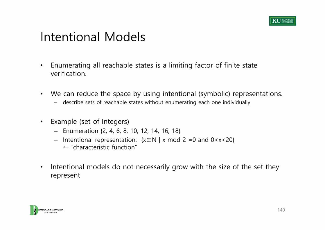
Intentional Models

• Enumerating all reachable states is a limiting factor of finite state verification.

• We can reduce the space by using intentional (symbolic) representations.– describe sets of reachable states without enumerating each one individually

• Example (set of Integers)– Enumeration {2, 4, 6, 8, 10, 12, 14, 16, 18}– Intentional representation: {x∈N | x mod 2 =0 and 0<x<20} ← “characteristic function”

• Intentional models do not necessarily grow with the size of the set they represent

140

OBDD: A Useful Intentional Model

• OBDD (Ordered Binary Decision Diagram)– A compact representation of Boolean functions

• Characteristic function for transition relations– Transitions = pairs of states– Function from pairs of states to Booleans is true, if there is a transition

between the pair.– Built iteratively by breadth-first expansion of the state space:

• Create a representation of the whole set of states reachable in k+1 steps from the set of states reachable in k steps

• OBDD stabilizes when all the transitions that can occur in the next step are already represented in the OBDD.

141

From OBDD to Symbolic Checking

• Intentional representation itself is not enough.• We must have an algorithm for determining whether it satisfies the

property we are checking.

• Example: A set of communicating state machines using OBDD– To represent the transition relation of a set of communicating state machines– To model a class of temporal logic specification formulas

• Combine OBDD representations of model and specification to produce a representation of just the set of transitions leading to a violation of the specification

– If the set is empty, the property has been verified.

142

Representing Transition Relations as Boolean Functions

• a b and cnot(a) or (b and c)

• BDD is a decision tree that has been transformed into an acyclic graph by merging nodes leading to identical sub-trees.

143

aF T

F T

bF T

cF T

Representing Transition Relations as Boolean Functions : Steps

A. Assign a label to each stateB. Encode transitions C. The transition tuples correspond

to paths leading to true, and all other paths lead to false.

144

s0 (00)

s1 (01)

b (x0=1)

a (x0=0)

0 0 0 0 0

0 0 0 1 1

x1 x2 x3 x4 x0

x00 1

x10 1

F T

x10 1

x20 1

x30 1

x40 1

x20 1

x30 1

x40 1

sym from state to state

(A)

(B)

(C)

s2 (10)

b (x0=1)

0 1 1 0 1

x30 1

Intentional vs. Explicit Representations

• Worst case:– Given a large set S of states,– a representation capable of distinguishing each subset of S cannot be more

compact on average than the representation that simply lists elements of the chosen subset.

• Intentional representations work well when they exploit structure and regularity of the state space.

145

Model Refinement

• Construction of finite state models – Should balance precision and efficiency

• Often the first model is unsatisfactory – Report potential failures that are obviously impossible– Exhaust resources before producing any result

• Minor differences in the model can have large effects on tractability of the verification procedure.

• Finite state verification as iterative process is required.

146

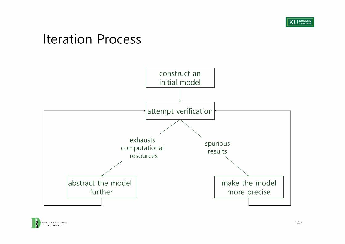
Iteration Process

147

construct aninitial model

attempt verification

abstract the model further

exhausts computational

resources

make the modelmore precise

spuriousresults

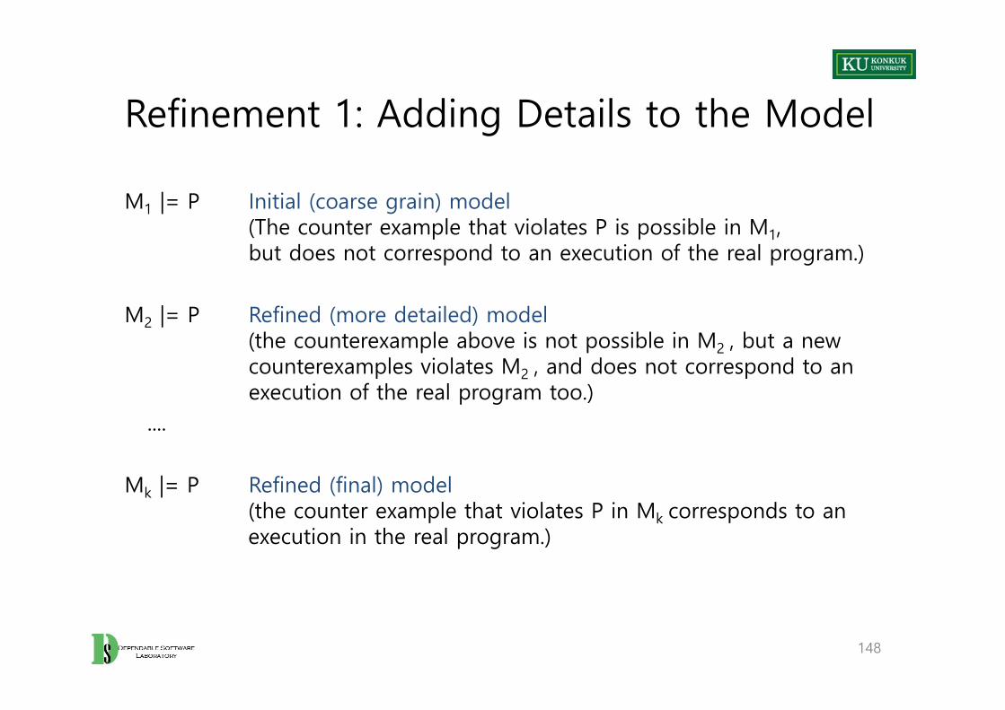
Refinement 1: Adding Details to the Model

M1 |= P Initial (coarse grain) model(The counter example that violates P is possible in M1, but does not correspond to an execution of the real program.)

M2 |= P Refined (more detailed) model(the counterexample above is not possible in M2 , but a newcounterexamples violates M2 , and does not correspond to anexecution of the real program too.)

....

Mk |= P Refined (final) model(the counter example that violates P in Mk corresponds to anexecution in the real program.)

148

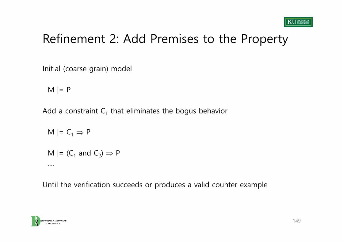
Refinement 2: Add Premises to the Property

Initial (coarse grain) model

M |= P

Add a constraint C1 that eliminates the bogus behavior

M |= C1 P

M |= (C1 and C2) P....

Until the verification succeeds or produces a valid counter example

149

Data Model Verification and Relational Algebra

• Another application of FSV, besides concurrent systems

• Many information systems are characterized by – Simple logic and algorithms– Complex data structures

• Key element of these systems is the data model (UML class and object diagrams + OCL assertions)= Sets of data and relations among them

• The challenge is to prove that – Individual constraints are consistent.– They ensure the desired properties of the system as a whole.

150

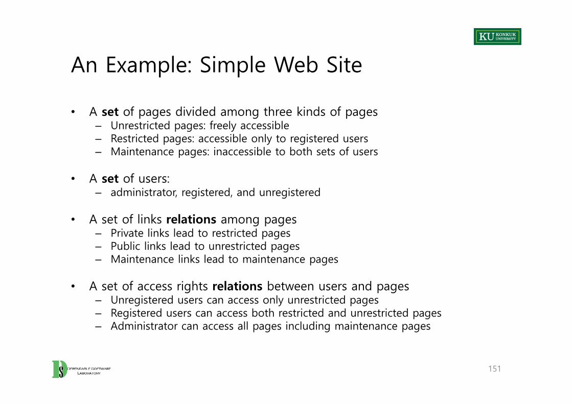
An Example: Simple Web Site

• A set of pages divided among three kinds of pages– Unrestricted pages: freely accessible– Restricted pages: accessible only to registered users– Maintenance pages: inaccessible to both sets of users

• A set of users: – administrator, registered, and unregistered

• A set of links relations among pages– Private links lead to restricted pages– Public links lead to unrestricted pages– Maintenance links lead to maintenance pages

• A set of access rights relations between users and pages– Unregistered users can access only unrestricted pages– Registered users can access both restricted and unrestricted pages– Administrator can access all pages including maintenance pages

151

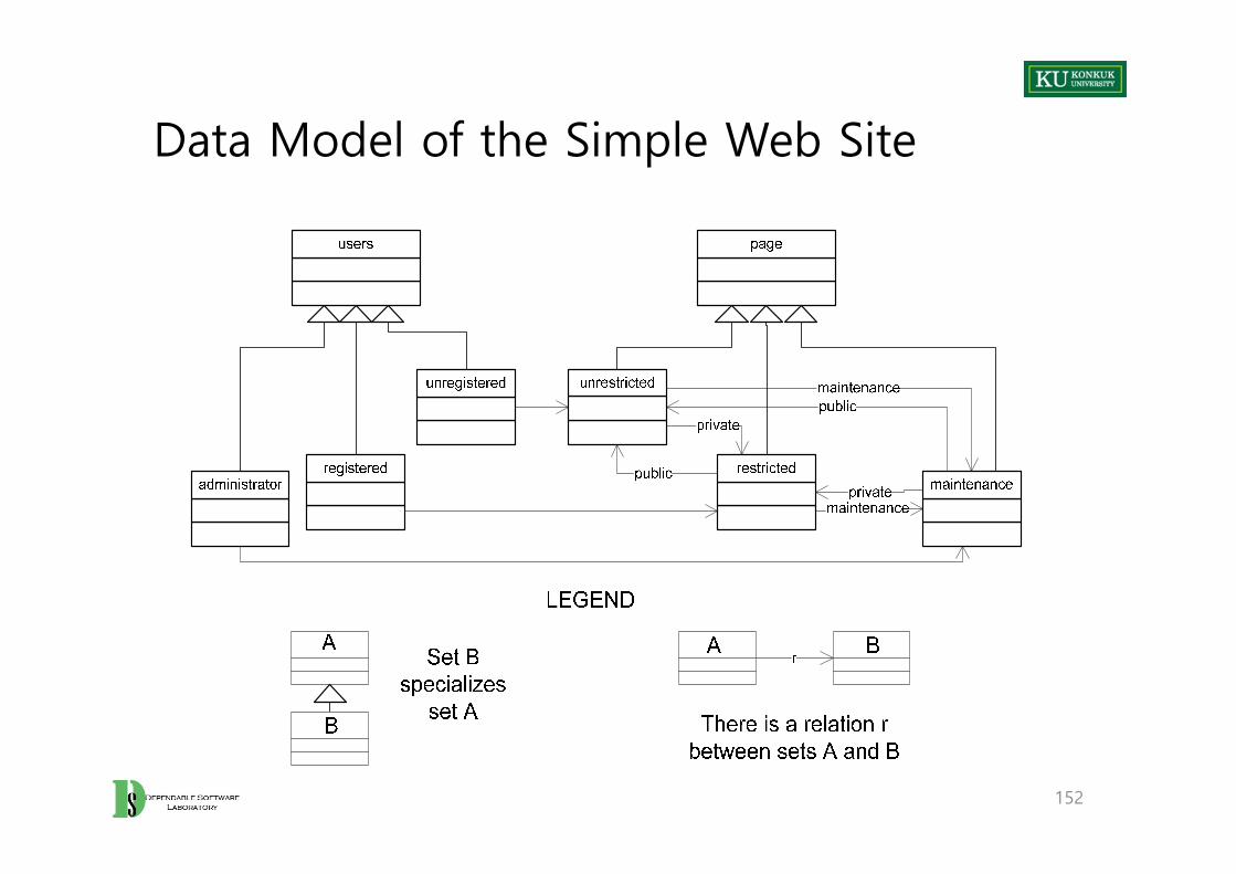
Data Model of the Simple Web Site

152

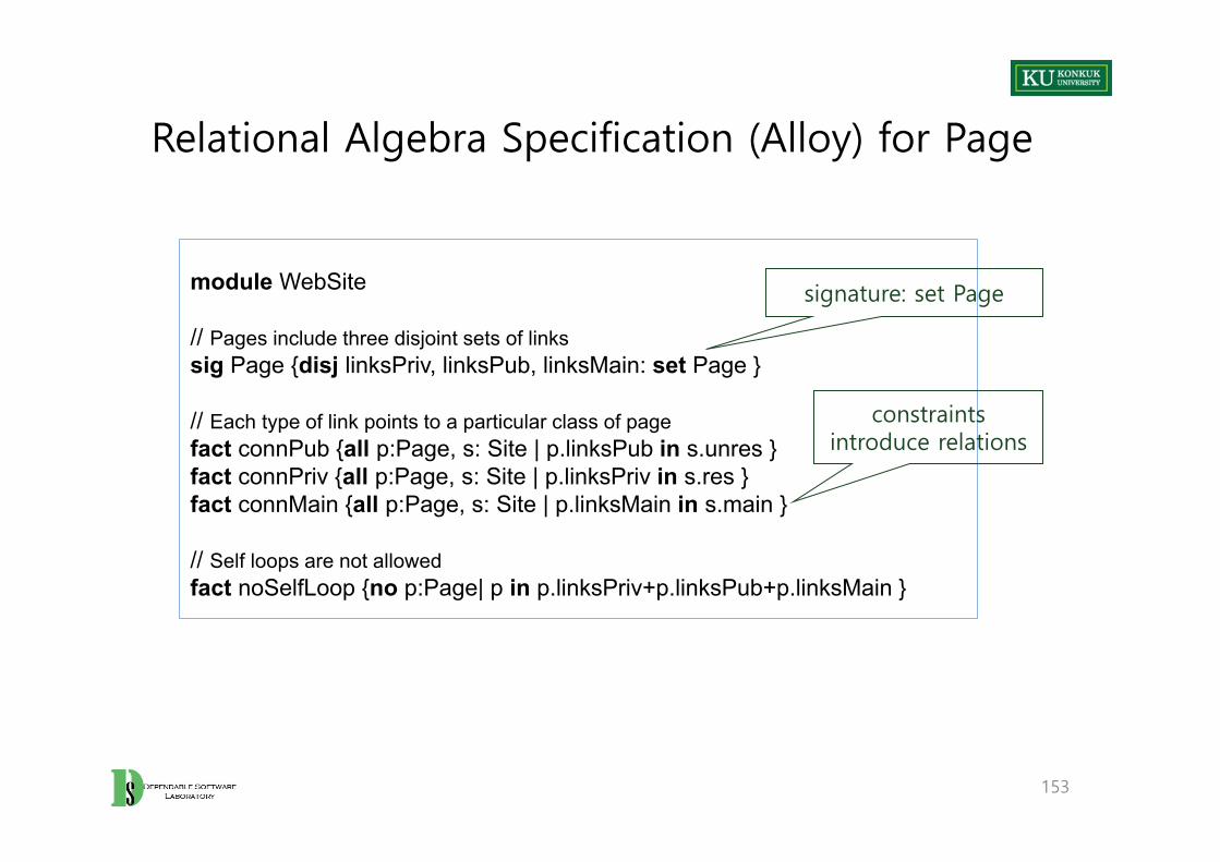
Relational Algebra Specification (Alloy) for Page

153

module WebSite

// Pages include three disjoint sets of links sig Page {disj linksPriv, linksPub, linksMain: set Page }

// Each type of link points to a particular class of page fact connPub {all p:Page, s: Site | p.linksPub in s.unres } fact connPriv {all p:Page, s: Site | p.linksPriv in s.res } fact connMain {all p:Page, s: Site | p.linksMain in s.main }

// Self loops are not allowed fact noSelfLoop {no p:Page| p in p.linksPriv+p.linksPub+p.linksMain }

signature: set Page

constraintsintroduce relations

Relational Algebra Specification (Alloy) for User

154

// Users are characterized by the set of pages that they can access sig User { pages: set Page } // Users are partitioned into three sets part sig Administrator, Registered, Unregistered extends User { }// Unregistered users can access only the home page, and unrestricted pagesfact accUnregistered {

all u: Unregistered, s: Site|u.pages = (s.home+s.unres) }// Registered users can access the home page,restricted and unrestricted pages fact accRegistered {

all u: Registered, s: Site|u.pages = (s.home+s.res+s.unres) }// Administrators can access all pages fact accAdministrator {

all u: Administrator, s: Site|u.pages = (s.home+s.res+s.unres+s.main)

}

Constraints mapusers to pages

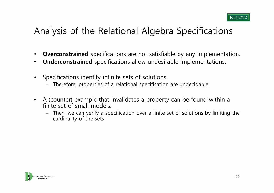
Analysis of the Relational Algebra Specifications

• Overconstrained specifications are not satisfiable by any implementation. • Underconstrained specifications allow undesirable implementations.

• Specifications identify infinite sets of solutions. – Therefore, properties of a relational specification are undecidable.

• A (counter) example that invalidates a property can be found within a finite set of small models.

– Then, we can verify a specification over a finite set of solutions by limiting the cardinality of the sets

155

Checking a Finite Set of Solutions

• If an example is found,– There are no logical contradictions in the model.– The solution is not overconstrained.

• If no counterexample of a property is found,– No reasonably small solution (property violation) exists. – BUT, NOT that NO solution exists.– We depend on a “small scope hypothesis”: Most bugs that can cause failure

with large collections of objects can also cause failure with very small collections. (so it’s worth looking for bugs in small collections even if we can’t afford to look in big ones)

156

Analysis of the Simple Web Site Specification

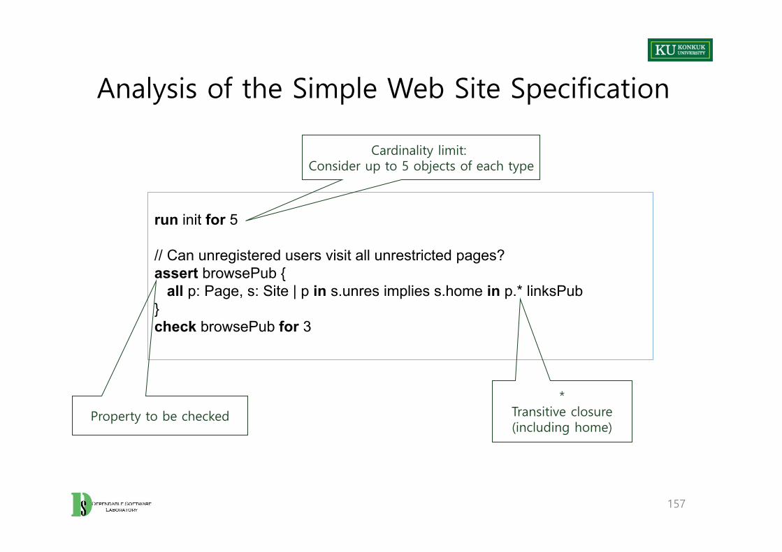
157

run init for 5

// Can unregistered users visit all unrestricted pages? assert browsePub {

all p: Page, s: Site | p in s.unres implies s.home in p.* linksPub}check browsePub for 3

Cardinality limit: Consider up to 5 objects of each type

Property to be checked

*Transitive closure(including home)

Analysis Result

Counterexample:

• Unregistered User_2 cannot visit the unrestricted page page_2.

• The only path from the home page to page_2 goes through the restricted page page_0.

• The property is violated because unrestricted browsing paths can be interrupted by restricted pages or pages under maintenance.

158

User_2

Page_1

pages

Page_2

pages

Page_0

linksPriv

linksPub

Site_0

home unres

unres

res

linksPub

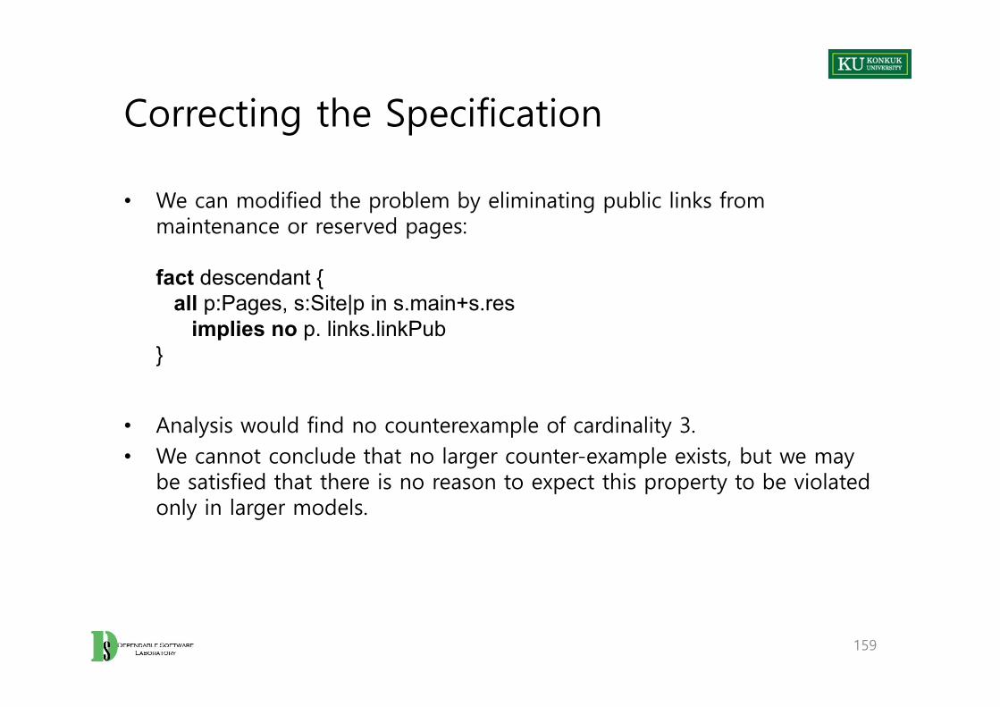
Correcting the Specification

• We can modified the problem by eliminating public links from maintenance or reserved pages:

fact descendant { all p:Pages, s:Site|p in s.main+s.res

implies no p. links.linkPub}

• Analysis would find no counterexample of cardinality 3.• We cannot conclude that no larger counter-example exists, but we may

be satisfied that there is no reason to expect this property to be violated only in larger models.

159

Summary

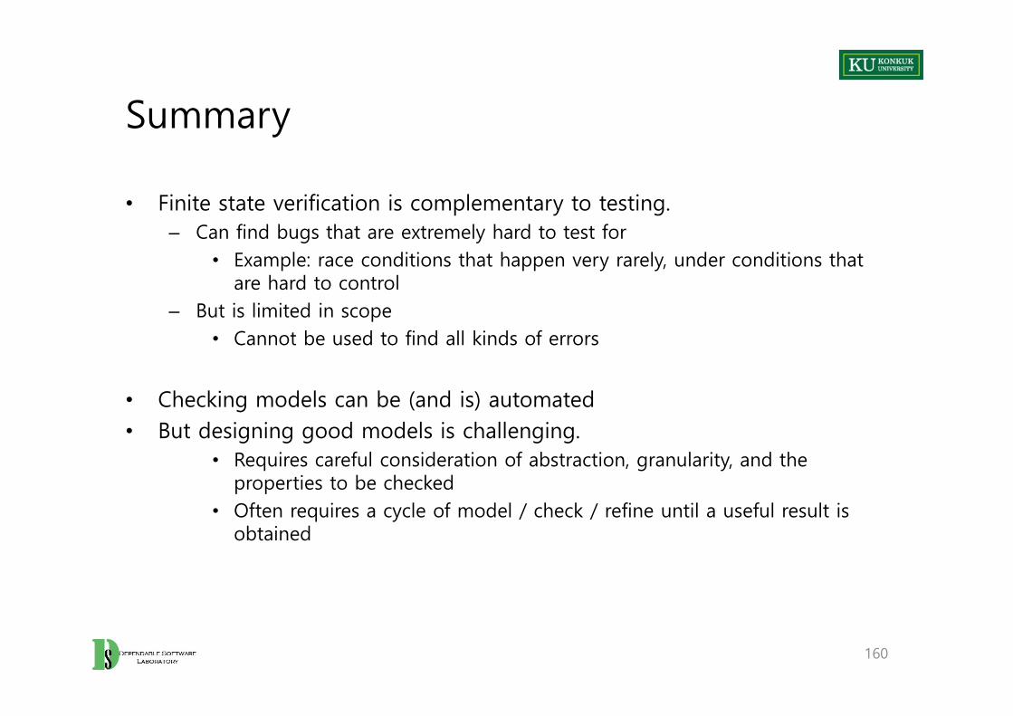
• Finite state verification is complementary to testing.– Can find bugs that are extremely hard to test for

• Example: race conditions that happen very rarely, under conditions that are hard to control

– But is limited in scope• Cannot be used to find all kinds of errors

• Checking models can be (and is) automated• But designing good models is challenging.

• Requires careful consideration of abstraction, granularity, and the properties to be checked

• Often requires a cycle of model / check / refine until a useful result is obtained

160

161

Part III. Problems and Methods

Chapter 9. Test Case Selection and Adequacy

Learning Objectives

• Understand the purpose of defining test adequacy criteria and their limitations

• Understand basic terminology of test selection and adequacy• Know some sources of information commonly used to define adequacy

criteria• Understand how test selection and adequacy criteria are used

164

Overview

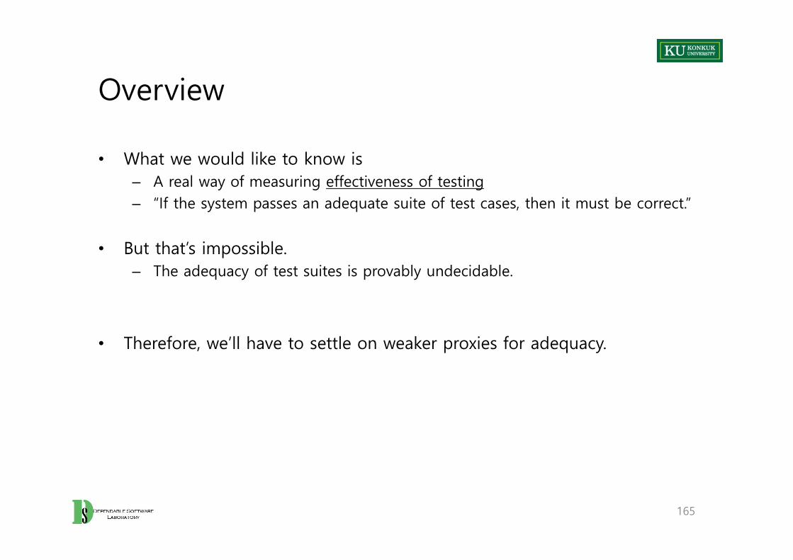
• What we would like to know is– A real way of measuring effectiveness of testing– “If the system passes an adequate suite of test cases, then it must be correct.”

• But that’s impossible.– The adequacy of test suites is provably undecidable.

• Therefore, we’ll have to settle on weaker proxies for adequacy.

165

Source of Test Specification

Testing Other namesSource of test specification

Example

Functional Testing

Black box testingSpecification-based testing

Software specification

If specification requires robust recovery from power failure, test obligations should include simulated power failure.

Structural Testing White box testing

Source code

Traverse each program loop one or more times

Model-based Testing

Models of system• Models used in specification or design• Models derived from source code

Exercise all transitions in communication protocol model

Fault-based Testing

Hypothesized faults, common bugs

Check for buffer overflow handling (common vulnerability) by testing on very large inputs

166

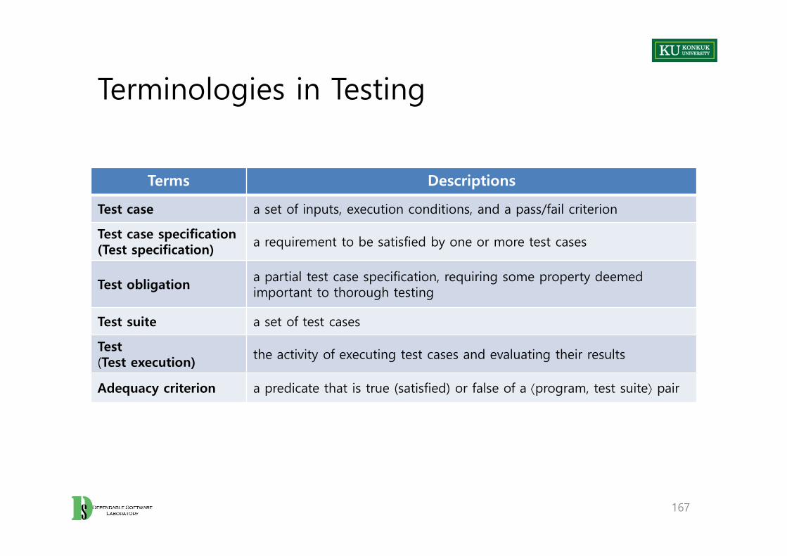
Terminologies in Testing

167

Terms Descriptions

Test case a set of inputs, execution conditions, and a pass/fail criterion

Test case specification (Test specification) a requirement to be satisfied by one or more test cases

Test obligation a partial test case specification, requiring some property deemed important to thorough testing

Test suite a set of test cases

Test (Test execution) the activity of executing test cases and evaluating their results

Adequacy criterion a predicate that is true (satisfied) or false of a program, test suite pair

Adequacy Criteria

• Adequacy criterion = Set of test obligations

• A test suite satisfies an adequacy criterion, iff– All the tests succeed (pass), and– Every test obligation in the criterion is satisfied by at least one of the test

cases in the test suite.

– Example: • “The statement coverage adequacy criterion is satisfied by test suite S for

program P, if each executable statement in P is executed by at least one test case in S, and the outcome of each test execution was pass.”

168

Satisfiability

• Sometimes no test suite can satisfy a criterion for a given program.– Example:

• Defensive programming style includes “can’t happen” sanity checks.– if (z < 0) {

throw new LogicError (“z must be positive here!”)}

• For this program, no test suite can satisfy statement coverage.

• Two ways of coping with the unsatisfiability of adequacy criteria1. Exclude any unsatisfiable obligation from the criterion2. Measure the extent to which a test suite approaches an adequacy criterion

169

Coping with the Unsatisfiability

• Approach A – Exclude any unsatisfiable obligation from the criterion– Example:

• Modify statement coverage to require execution only of statements which can be executed

– But, we can’t know for sure which are executable or not.

• Approach B – Measure the extent to which a test suite approaches an adequacy criterion– Example

• If a test suite satisfies 85 of 100 obligations, we have reached 85% coverage.

– Terms: • An adequacy criterion is satisfied or not.• A coverage measure is the fraction of satisfied obligations.

170

Coverage

• Measuring coverage (% of satisfied test obligations) can be a useful indicator of – Progress toward a thorough test suite (thoroughness of test suite)

– Trouble spots requiring more attention in testing

• But, coverage is only a proxy for thoroughness or adequacy.– It’s easy to improve coverage without improving a test suite (much easier

than designing good test cases)– The only measure that really matters is (cost-) effectiveness.

171

Comparing Criteria

• Can we distinguish stronger from weaker adequacy criteria?

• Analytical approach– Describe conditions under which one adequacy criterion is provably stronger

than another– Just a piece of the overall “effectiveness” question– Stronger = gives stronger guarantees

→ Subsumes relation

172

Subsumes Relation

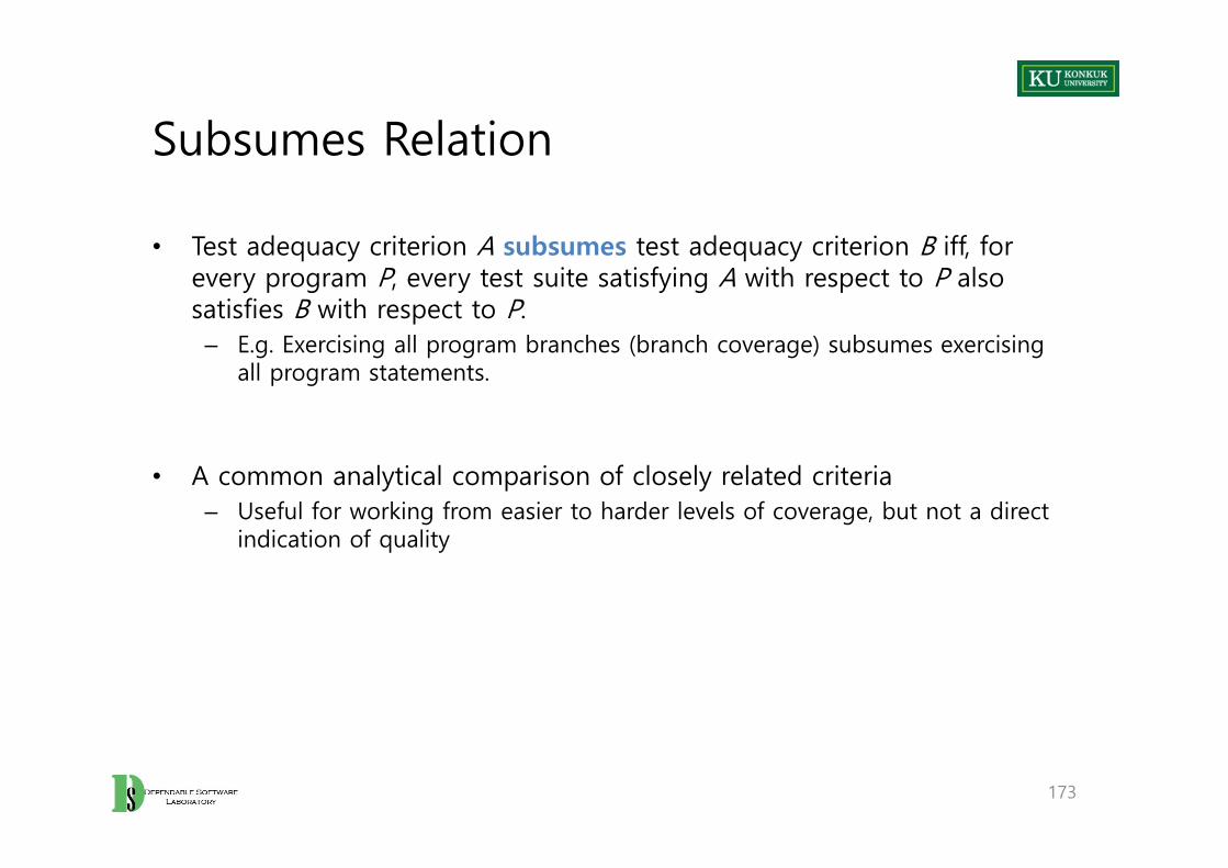
• Test adequacy criterion A subsumes test adequacy criterion B iff, for every program P, every test suite satisfying A with respect to P also satisfies B with respect to P.

– E.g. Exercising all program branches (branch coverage) subsumes exercising all program statements.

• A common analytical comparison of closely related criteria– Useful for working from easier to harder levels of coverage, but not a direct

indication of quality

173

174

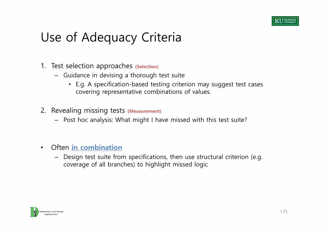
Use of Adequacy Criteria

1. Test selection approaches (Selection)

– Guidance in devising a thorough test suite• E.g. A specification-based testing criterion may suggest test cases

covering representative combinations of values.

2. Revealing missing tests (Measurement)

– Post hoc analysis: What might I have missed with this test suite?

• Often in combination– Design test suite from specifications, then use structural criterion (e.g.

coverage of all branches) to highlight missed logic

175

Summary

• Adequacy criteria provide a way to define a notion of “thoroughness” in a test suite.

– But, they don’t offer guarantees.– More like rules to highlight inadequacy

• Adequacy criteria are defined in terms of “covering” some information– Derived from many sources(specs, code, models, etc.)

• Adequacy criteria may be used for selection as well as measurement. – But, an aid to thoughtful test design, not a substitute

176

177

Chapter 10. Functional Testing

Learning Objectives

• Understand the rationale for systematic (non-random) selection of test cases

• Understand why functional test selection is a primary, base-line technique

• Distinguish functional testing from other systematic testing techniques

179

Functional Testing

• Functional testing– Deriving test cases from program specifications – ‘Functional’ refers to the source of information used in test case design, not

to what is tested.

• Also known as:– Specification-based testing (from specifications)– Black-box testing (no view of source code)

• Functional specification = description of intended program behavior– Formal or informal

180

Systematic testing vs. Random testing

• Random (uniform) testing– Pick possible inputs uniformly– Avoids designer’s bias– But, treats all inputs as equally valuable

• Systematic (non-uniform) testing– Try to select inputs that are especially valuable– Usually by choosing representatives of classes that are apt to fail often or not

at all

• Functional testing is a systematic (partition-based) testing strategy.

181

Why Not Random Testing?

• Due to non-uniform distribution of faults– Example:

• Java class “roots” applies quadratic equation

– Supposed an incomplete implementation logic: • Program does not properly handle the case in which b2 - 4ac =0 and a=0

– Failing values are sparse in the input space: needles in a very big haystack– Random sampling is unlikely to choose a=0 and b=0.

182

Purpose of Testing

• Our goal is to find needles and remove them from hay. → Look systematically (non-uniformly) for needles !!!– We need to use everything we know about needles.

• E.g. Are they heavier than hay? Do they sift to the bottom?

• To estimate the proportion of needles to hay → Sample randomly !!!– Reliability estimation requires unbiased samples for valid statistics. – But that’s not our goal.

183

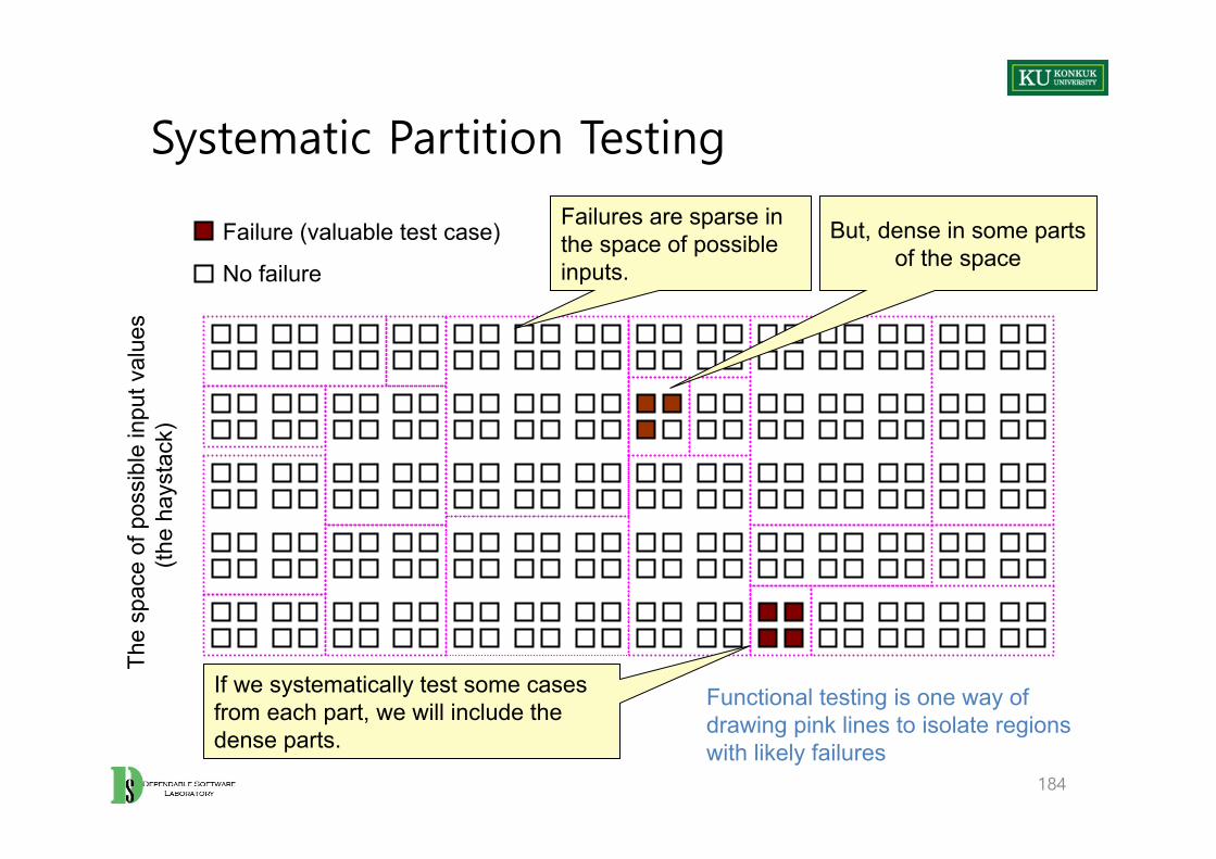
Systematic Partition Testing

184

Failure (valuable test case)

No failure

Failures are sparse in the space of possible inputs.

But, dense in some parts of the space

If we systematically test some cases from each part, we will include the dense parts.

Functional testing is one way of drawing pink lines to isolate regions with likely failures

The

spac

e of

pos

sibl

e in

put v

alue

s(th

e ha

ysta

ck)

Principles of Systematic Partitioning

• Exploit some knowledge to choose samples that are more likely to include “special” or “trouble-prone” regions of the input space

– Failures are sparse in the whole input space.– But, we may find regions in which they are dense.

• (Quasi-) Partition testing: separates the input space into classes whose union is the entire space

• Desirable case: Each fault leads to failures that are dense (easy to find) in some class of inputs

– Sampling each class in the quasi-partition selects at least one input that leads to a failure, revealing the fault.

– Seldom guaranteed; We depend on experience-based heuristics.

185

A Systematic Approach: Functional Testing

• Functional testing uses the specification (formal or informal) to partition the input space.

– E.g. Specification of “roots” program suggests division between cases with zero, one, and two real roots.

• Test each category and boundaries between categories– No guarantees, but experience suggests failures often lie at the boundaries.

(as in the “roots” program)

• Functional Testing is a base-line technique for designing test cases.

186

Functional Testing

• The base-line technique for designing test cases– Timely

• Often useful in refining specifications and assessing testability before code is written

– Effective• Find some classes of fault (e.g. missing logic) that can elude other

approaches– Widely applicable

• To any description of program behavior serving as specification• At any level of granularity from module to system testing

– Economical• Typically less expensive to design and execute than structural (code-

based) test cases

187

Functional Test vs. Structural Test

• Different testing strategies are most effective for different classes of faults.

• Functional testing is best for missing logic faults.– A common problem: Some program logic was simply forgotten.– Structural (code-based) testing will never focus on code that isn’t there.

• Functional test applies at all granularity levels– Unit (from module interface spec)– Integration (from API or subsystem spec)– System (from system requirements spec)– Regression (from system requirements + bug history)

• Structural test design applies to relatively small parts of a system– Unit and integration testing

188

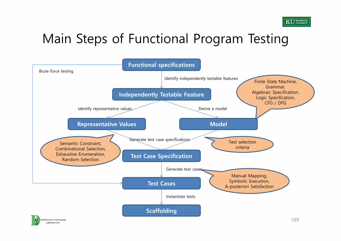
Main Steps of Functional Program Testing

189

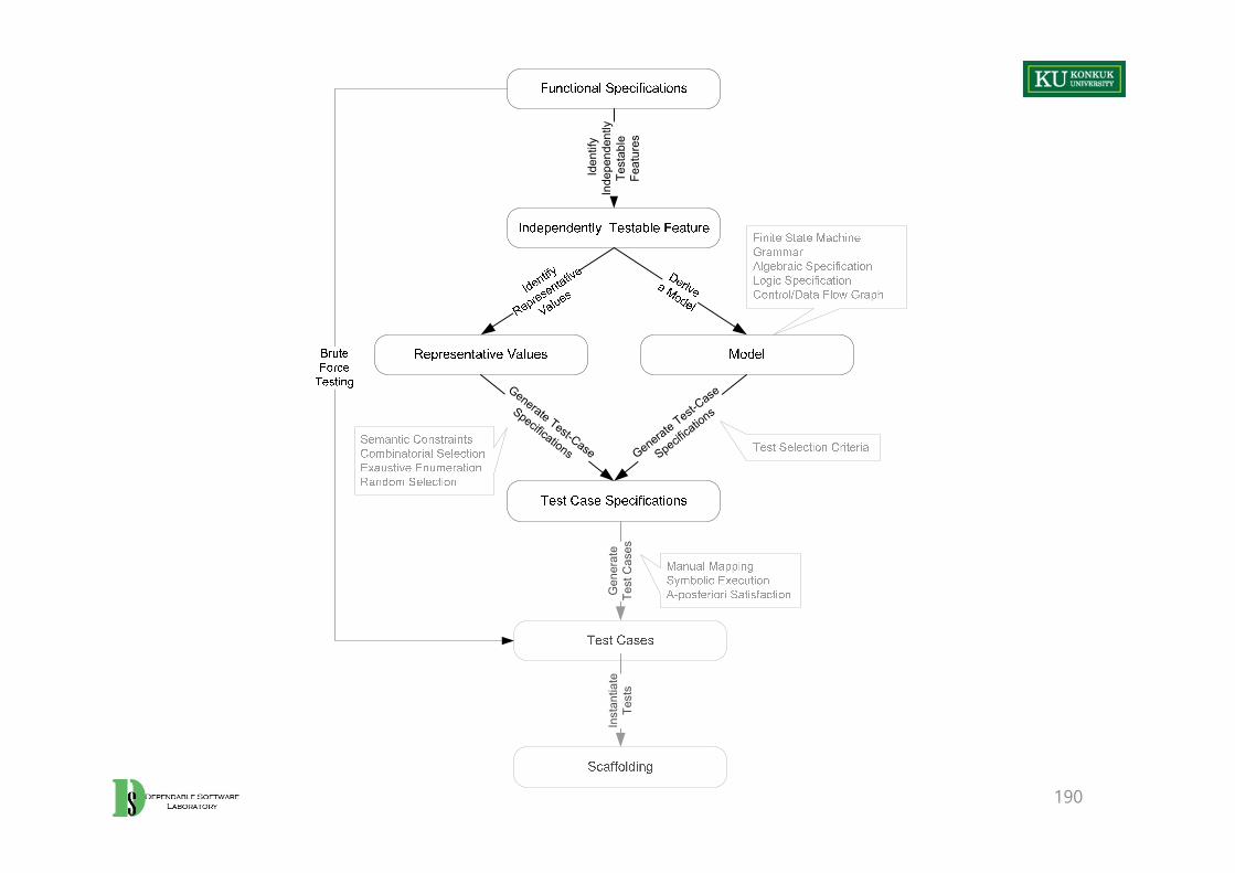
Functional specifications

Independently Testable Feature

Representative Values Model

Test Case Specification

Test Cases

Scaffolding

Identify independently testable features

Derive a modelIdentify representative values

Generate test case specifications

Generate test cases

Instantiate tests

Finite State Machine,Grammar,

Algebraic Specification,Logic Specification,

CFG / DFG

Test selection criteria

Manual Mapping,Symbolic Execution,

A-posteriori Satisfaction

Semantic Constraint,Combinational Selection,Exhaustive Enumeration,

Random Selection

Brute force testing

190

Iden

tify

Inde

pend

ently

Te

stab

le

Feat

ures

Generate Test-Case

Specifications Generate Test-Case

Specifications

Gen

erat

e Te

st C

ases

Inst

antia

teTe

sts

From Specifications to Test Cases

1. Identify independently testable features– If the specification is large, break it into independently testable features.

2. Identify representative classes of values, or derive a model of behavior– Often simple input/output transformations don’t describe a system. – We use models in program specification, in program design, and in test

design too.

3. Generate test case specifications– Typically, combinations of input values or model behaviors

4. Generate test cases and instantiate tests

191

Summary

• Functional testing (generating test cases from specifications) is a valuable and flexible approach to software testing.

– Applicable from very early system specifications right through module specifications

• Partition testing suggests dividing the input space into equivalent classes.– Systematic testing is intentionally non-uniform to address special cases, error

conditions and other small places.– Dividing a big haystack into small and hopefully uniform piles where the

needles might be concentrated

192

193

Chapter 11. Combinatorial Testing

Learning Objectives

• Understand three key ideas in combinatorial approaches– Category-partition testing– Pairwise testing – Catalog-based testing

195

Overview

• Combinatorial testing identifies distinct attributes that can be varied. – In data, environment or configuration– Example:

• Browser could be “IE” or “Firefox”• Operating system could be “Vista”, “XP” or “OSX”

• Combinatorial testing systematically generates combinations to be tested.– Example:

• IE on Vista, IE on XP, Firefox on Vista, Firefox on OSX, etc.

• Rationale: – Test cases should be varied and include possible “corner cases”.

196

Key Ideas in Combinatorial Approaches

1. Category-partition testing– Separate (manual) identification of values that characterize the input space

from (automatic) generation of combinations for test cases

2. Pairwise testing – Systematically test interactions among attributes of the program input space

with a relatively small number of test cases

3. Catalog-based testing– Aggregate and synthesize the experience of test designers in a particular

organization or application domain, to aid in identifying attribute values

197

1. Category-Partition Testing

1. Decompose the specification into independently testable features– for each feature, identify parameters and environment elements– for each parameter and environment element, identify elementary

characteristics (→ categories)

2. Identify representative values– for each characteristic(category), identify classes of values

• normal values• boundary values• special values• error values

3. Generate test case specifications

198

An Example: “Check Configuration”

• In the Web site of a computer manufacturer, i.e. Dell, ‘checking configuration’ checks the validity of a computer configuration.

– Two parameters:• Model• Set of Components

199

Informal Specification of ‘Model’

200

Model: A model identifies a specific product and determines a set of constraints on available components. Models are characterized by logical slots for components, which may or may not be implemented by physical slots on a bus. Slots may be required or optional. Required slots must be assigned with a suitable component to obtain a legal configuration, while optional slots may be left empty or filled depending on the customer’s needs.

Example: The required “slots” of the Chipmunk C20 laptop computer include a screen, a processor, a hard disk, memory, and an operating system. (Of these, only the hard disk and memory are implemented using actual hardware slots on a bus.) The optional slots include external storage devices such as a CD/DVD writer.

Informal Specification of ‘Set of Component’

201

Set of Components: A set of (slot, component) pairs, corresponds to the required and optional slots of the model. A component is a choice that can be varied within a model, and which is not designed to be replaced by the end user. Available components and a default for each slot is determined by the model. The special value empty is allowed (and may be the default selection) for optional slots. In addition to being compatible or incompatible with a particular model and slot, individual components may be compatible or incompatible with each other.

Example: The default configuration of the Chipmunk C20 includes 20 gigabytes of hard disk; 30 and 40 gigabyte disks are also available. (Since the hard disk is a required slot, empty is not an allowed choice.) The default operating system is RodentOS 3.2, personal edition, but RodentOS 3.2 mobile server edition may also be selected. The mobile server edition requires at least 30 gigabytes of hard disk.

Step 1: Identify Independently Testable Features and Parameter Characteristics

• Choosing categories– No hard-and-fast rules for choosing categories!– Not a trivial task

• Categories reflect test designer's judgment. – Which classes of values may be treated differently by an implementation.

• Choosing categories well requires experience and knowledge of the application domain and product architecture.

202

Identify Independently Testable Units

Model

Model number

Number of required slots for selected model (#SMRS)

Number of optional slots for selected model (#SMOS)

203

Components

Correspondence of selection with model slots

Number of required components with selection empty

Required component selection

Number of optional components with selection empty

Optional component selection

Product Database

Number of models in database (#DBM)

Number of components in database (#DBC)

Parameters Categories

Step 2: Identify Representative Values

• Identify representative classes of values for each of the categories

• Representative values may be identified by applying – Boundary value testing

• Select extreme values within a class • Select values outside but as close as possible to the class• Select interior (non-extreme) values of the class

– Erroneous condition testing• Select values outside the normal domain of the program

204

Representative Values: Model

• Model numberMalformedNot in databaseValid

• Number of required slots for selected model (#SMRS)01Many

• Number of optional slots for selected model (#SMOS)01Many

205

Representative Values: Components

• Correspondence of selection with model slotsOmitted slotsExtra slotsMismatched slotsComplete correspondence

• Number of required components with non empty selection0< number required slots= number required slots

• Required component selectionSome defaultsAll valid 1 incompatible with slots 1 incompatible with another selection 1 incompatible with model 1 not in database

206

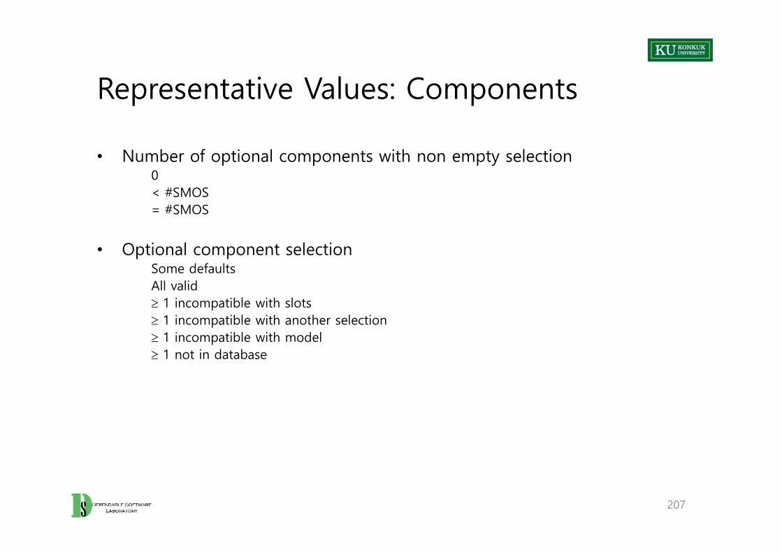
Representative Values: Components

• Number of optional components with non empty selection0< #SMOS= #SMOS

• Optional component selectionSome defaultsAll valid 1 incompatible with slots 1 incompatible with another selection 1 incompatible with model 1 not in database

207

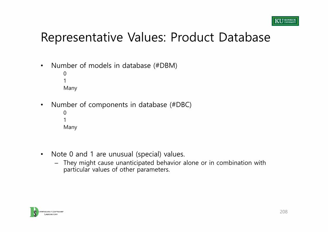
Representative Values: Product Database

• Number of models in database (#DBM)01Many

• Number of components in database (#DBC)01Many

• Note 0 and 1 are unusual (special) values. – They might cause unanticipated behavior alone or in combination with

particular values of other parameters.

208

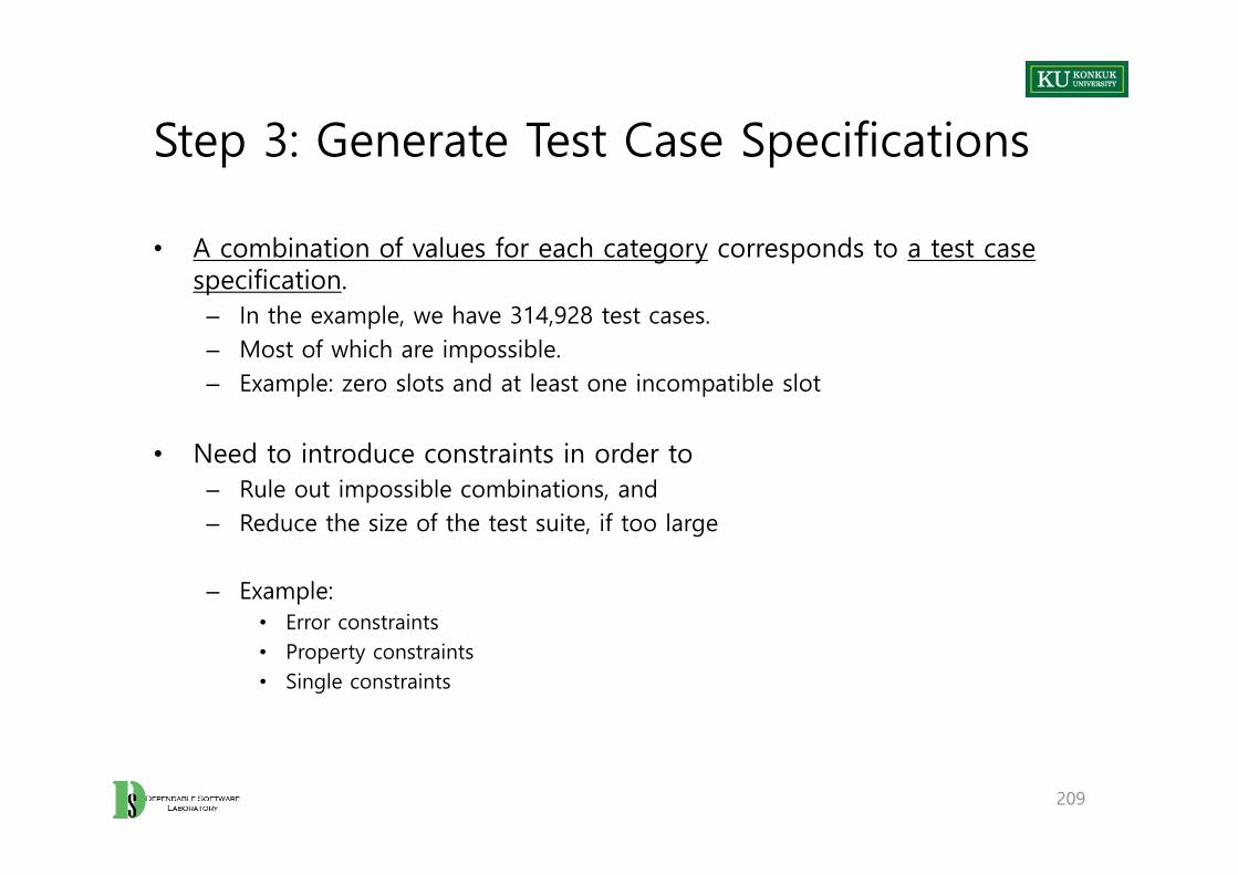
Step 3: Generate Test Case Specifications

• A combination of values for each category corresponds to a test case specification.

– In the example, we have 314,928 test cases.– Most of which are impossible.– Example: zero slots and at least one incompatible slot

• Need to introduce constraints in order to– Rule out impossible combinations, and– Reduce the size of the test suite, if too large

– Example:• Error constraints• Property constraints• Single constraints

209

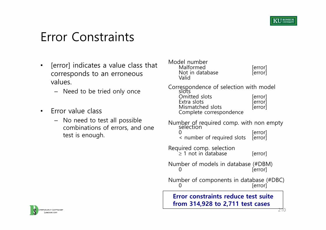
Error Constraints

• [error] indicates a value class that corresponds to an erroneous values.

– Need to be tried only once

• Error value class– No need to test all possible

combinations of errors, and one test is enough.

Model numberMalformed [error]Not in database [error]Valid

Correspondence of selection with model slotsOmitted slots [error]Extra slots [error]Mismatched slots [error]Complete correspondence

Number of required comp. with non empty selection0 [error]< number of required slots [error]

Required comp. selection 1 not in database [error]

Number of models in database (#DBM)0 [error]

Number of components in database (#DBC)0 [error]

210

Error constraints reduce test suite from 314,928 to 2,711 test cases

Property Constraints

• Constraint [property] [if-property] rule out invalid combinations of values.– [property] groups values of a single parameter to identify subsets of values

with common properties.– [if-property] bounds the choices of values for a category that can be

combined with a particular value selected for a different category.

211

Property Constraints

Number of required slots for selected model (#SMRS)1 [property RSNE]Many [property RSNE] [property RSMANY]

Number of optional slots for selected model (#SMOS)1 [property OSNE]Many [property OSNE] [property OSMANY]

Number of required comp. with non empty selection0 [if RSNE] [error]< number required slots [if RSNE] [error]= number required slots [if RSMANY]

Number of optional comp. with non empty selection< number required slots [if OSNE]= number required slots [if OSMANY]

212

from 2,711 to 908 test cases

Single Constraints

• [single] indicates a value class that test designers choose to test only once to reduce the number of test cases.

• Example– Value some default for required component selection and optional

component selection may be tested only once despite not being an erroneous condition.

• Note – Single and error have the same effect but differ in rationale. – Keeping them distinct is important for documentation and regression testing.

213

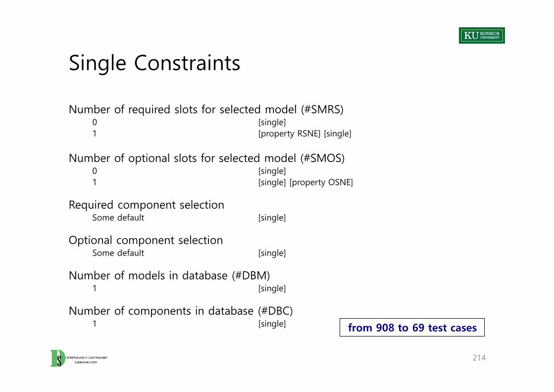
Single Constraints

Number of required slots for selected model (#SMRS)0 [single]1 [property RSNE] [single]

Number of optional slots for selected model (#SMOS)0 [single]1 [single] [property OSNE]

Required component selectionSome default [single]

Optional component selectionSome default [single]

Number of models in database (#DBM)1 [single]

Number of components in database (#DBC)1 [single]

214

from 908 to 69 test cases

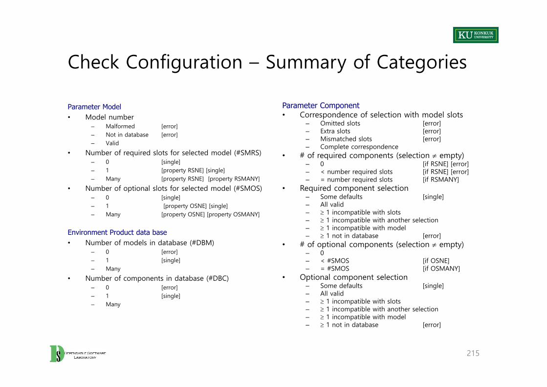
Check Configuration – Summary of Categories

Parameter Model• Model number

– Malformed [error]– Not in database [error]– Valid

• Number of required slots for selected model (#SMRS)– 0 [single]– 1 [property RSNE] [single] – Many [property RSNE] [property RSMANY]

• Number of optional slots for selected model (#SMOS)– 0 [single]– 1 [property OSNE] [single] – Many [property OSNE] [property OSMANY]

Environment Product data base• Number of models in database (#DBM)

– 0 [error]– 1 [single]– Many

• Number of components in database (#DBC)– 0 [error]– 1 [single]– Many

Parameter Component• Correspondence of selection with model slots

– Omitted slots [error]– Extra slots [error]– Mismatched slots [error]– Complete correspondence

• # of required components (selection empty)– 0 [if RSNE] [error]– < number required slots [if RSNE] [error]– = number required slots [if RSMANY]

• Required component selection– Some defaults [single]– All valid– 1 incompatible with slots– 1 incompatible with another selection– 1 incompatible with model– 1 not in database [error]

• # of optional components (selection empty)– 0– < #SMOS [if OSNE]– = #SMOS [if OSMANY]

• Optional component selection– Some defaults [single]– All valid– 1 incompatible with slots– 1 incompatible with another selection– 1 incompatible with model– 1 not in database [error]

215

Category-Partitioning Testing, in Summary

• Category partition testing gives us systematic approaches to – Identify characteristics and values (the creative step)– Generate combinations (the mechanical step)

• But, test suite size grows very rapidly with number of categories. • Pairwise (and n-way) combinatorial testing is a non-exhaustive approach.

– Combine values systematically but not exhaustively

216

2. Pairwise Combination Testing

• Category partition works well when intuitive constraints reduce the number of combinations to a small amount of test cases.

– Without many constraints, the number of combinations may be unmanageable.

• Pairwise combination– Instead of exhaustive combinations– Generate combinations that efficiently cover all pairs (triples,…) of classes– Rationale:

• Most failures are triggered by single values or combinations of a few values.• Covering pairs (triples,…) reduces the number of test cases, but reveals most faults.

217

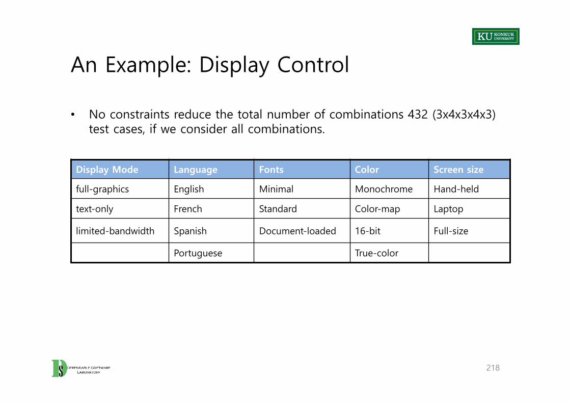
An Example: Display Control

• No constraints reduce the total number of combinations 432 (3x4x3x4x3) test cases, if we consider all combinations.

218

Display Mode Language Fonts Color Screen size

full-graphics English Minimal Monochrome Hand-held

text-only French Standard Color-map Laptop

limited-bandwidth Spanish Document-loaded 16-bit Full-size

Portuguese True-color

Pairwise Combination: 17 Test Cases

219

Language Color Display Mode Fonts Screen Size

English Monochrome Full-graphics Minimal Hand-held

English Color-map Text-only Standard Full-size

English 16-bit Limited-bandwidth - Full-size

English True-color Text-only Document-loaded Laptop

French Monochrome Limited-bandwidth Standard Laptop

French Color-map Full-graphics Document-loaded Full-size

French 16-bit Text-only Minimal -

French True-color - - Hand-held

Spanish Monochrome - Document-loaded Full-size

Spanish Color-map Limited-bandwidth Minimal Hand-held

Spanish 16-bit Full-graphics Standard Laptop

Spanish True-color Text-only - Hand-held

Portuguese - - Monochrome Text-only

Portuguese Color-map - Minimal Laptop

Portuguese 16-bit Limited-bandwidth Document-loaded Hand-held

Portuguese True-color Full-graphics Minimal Full-size

Portuguese True-color Limited-bandwidth Standard Hand-held

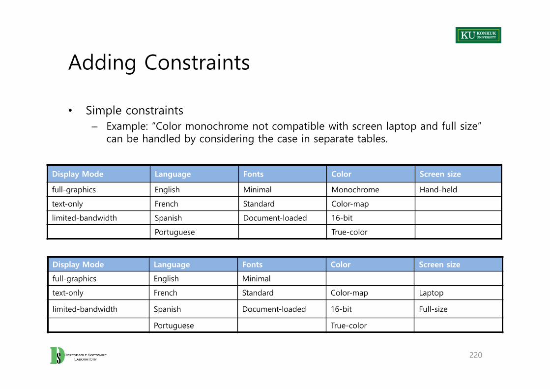
Adding Constraints

• Simple constraints– Example: “Color monochrome not compatible with screen laptop and full size”

can be handled by considering the case in separate tables.

220

Display Mode Language Fonts Color Screen size

full-graphics English Minimal Monochrome Hand-held

text-only French Standard Color-map

limited-bandwidth Spanish Document-loaded 16-bit

Portuguese True-color

Display Mode Language Fonts Color Screen size

full-graphics English Minimal

text-only French Standard Color-map Laptop

limited-bandwidth Spanish Document-loaded 16-bit Full-size

Portuguese True-color

Pairwise Combination Testing, in Summary

• Category-partition approach gives us– Separation between (manual) identification of parameter characteristics and

values, and (automatic) generation of test cases that combine them– Constraints to reduce the number of combinations

• Pairwise (or n-way) testing gives us – Much smaller test suites, even without constraints– But, we can still use constraints.

• We still need help to make the manual step more systematic.

221

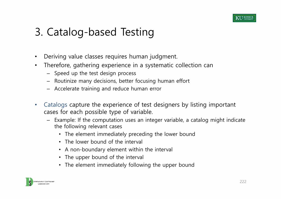
3. Catalog-based Testing

• Deriving value classes requires human judgment. • Therefore, gathering experience in a systematic collection can

– Speed up the test design process – Routinize many decisions, better focusing human effort– Accelerate training and reduce human error

• Catalogs capture the experience of test designers by listing important cases for each possible type of variable.

– Example: If the computation uses an integer variable, a catalog might indicate the following relevant cases

• The element immediately preceding the lower bound • The lower bound of the interval• A non-boundary element within the interval• The upper bound of the interval• The element immediately following the upper bound

222

Catalog-based Testing Process

1. Identify elementary items of the specification– Pre-conditions– Post-conditions– Definitions– Variables– Operations

2. Derive a first set of test case specifications from pre-conditions, post-conditions and definitions

3. Complete the set of test case specifications using test catalogs

223

An Example: ‘cgi_decode’

• An informal specification of ‘cgi_decode’

224

Function cgi_decode translates a cgi-encoded string to a plain ASCII string, reversing the encoding applied by the common gateway interface (CGI) of most web servers.

CGI translates spaces to +, and translates most other non-alphanumeric characters to hexadecimal escape sequences.

cgi_decode maps + to spaces, %xy (where x and y are hexadecimal digits) to the corresponding ASCII character, and other alphanumeric characters to themselves.

‘cgi_digicode’ Input/Output

• [INPUT]: encoded A string of characters (the input CGI sequence) containing below and terminated by a null character

– alphanumeric characters– the character +– the substring “%xy” , where x and y are hexadecimal digits

• [OUTPUT]: decoded A string of characters (the plain ASCII characters corresponding to the input CGI sequence)

– alphanumeric characters copied into output (in corresponding positions)– blank for each ‘+’ character in the input– single ASCII character with value xy for each substring “%xy”

• [OUTPUT]: return value cgi_decode returns– 0 for success – 1 if the input is malformed

225

‘cgi_digicode’ Definitions

• Pre-conditions: Conditions on inputs that must be true before the execution

– Validated preconditions: checked by the system– Assumed preconditions: assumed by the system

• Post-conditions: Results of the execution

• Variables: Elements used for the computation

• Operations: Main operations on variables and inputs

• Definitions: Abbreviations

226

Step 1: Identify Elementary Items of the SpecificationVAR 1 encoded: a string of ASCII charactersVAR 2 decoded: a string of ASCII charactersVAR 3 return value: a boolean

DEF 1 hexadecimal characters, in range ['0' .. '9', 'A' .. 'F', 'a' .. 'f']DEF 2 sequences %xy, where x and y are hexadecimal charactersDEF 3 CGI items as alphanumeric character, or '+', or CGI hexadecimal

OP 1 Scan the input string encoded

PRE 1 (Assumed) input string encoded null-terminated string of charsPRE 2 (Validated) input string encoded sequence of CGI items

POST 1 if encoded contains alphanumeric characters, they are copied to the output stringPOST 2 if encoded contains characters +, they are replaced in the output string by ASCII SPACE

characters POST 3 if encoded contains CGI hexadecimals, they are replaced by the corresponding ASCII charactersPOST 4 if encoded is processed correctly, it returns 0POST 5 if encoded contains a wrong CGI hexadecimal (a substring xy, where either x or y are absent or

are not hexadecimal digits, cgi_decode returns 1 POST 6 if encoded contains any illegal character, it returns 1VAR 1 encoded: a string of ASCII characters

227

Step 2: Derive an Initial Set of Test Case Specifications

• Validated preconditions:– Simple precondition (expression without operators)

• 2 classes of inputs: – inputs that satisfy the precondition– inputs that do not satisfy the precondition

– Compound precondition (with AND or OR):• apply modified condition/decision (MC/DC) criterion

• Assumed precondition:– apply MC/DC only to “OR preconditions”

• Postconditions and Definitions: – if given as conditional expressions, consider conditions as if they were

validated preconditions

228

Test Cases from PRE

PRE 2 (Validated): the input string encoded is a sequence of CGI items – TC-PRE2-1: encoded is a sequence of CGI items – TC-PRE2-2: encoded is not a sequence of CGI items

POST 1: if encoded contains alphanumeric characters, they are copied in the output string in the corresponding position

– TC-POST1-1: encoded contains alphanumeric characters – TC-POST1-2: encoded does not contain alphanumeric characters

POST 2: if encoded contains characters +, they are replaced in the output string by ASCII SPACE characters

– TC-POST2-1: encoded contains character +– TC-POST2-2: encoded does not contain character +

229

Test Cases from POST

POST 3: if encoded contains CGI hexadecimals, they are replaced by the corresponding ASCII characters

– TC-POST3-1 Encoded: contains CGI hexadecimals – TC-POST3-2 Encoded: does not contain a CGI hexadecimal

POST 4: if encoded is processed correctly, it returns 0

POST 5: if encoded contains a wrong CGI hexadecimal (a substring xy, where either x or y are absent or are not hexadecimal digits, cgi_decode returns 1

– TC-POST5-1 Encoded: contains erroneous CGI hexadecimals

POST 6 if encoded contains any illegal character, it returns 1– TC-POST6-1 Encoded: contains illegal characters

230

Step 3: Complete the Test Case Specification using Catalog

• Scan the catalog sequentially – For each element of the catalog,

• Scan the specifications and apply the catalog entry

• Delete redundant test cases

• Catalog– List of kinds of elements that can occur in a specification– Each catalog entry is associated with a list of generic test case specifications.

• Example: Catalog entry Boolean – Two test case specifications: true, false– Label in/out indicate if applicable only to input, output, both

231

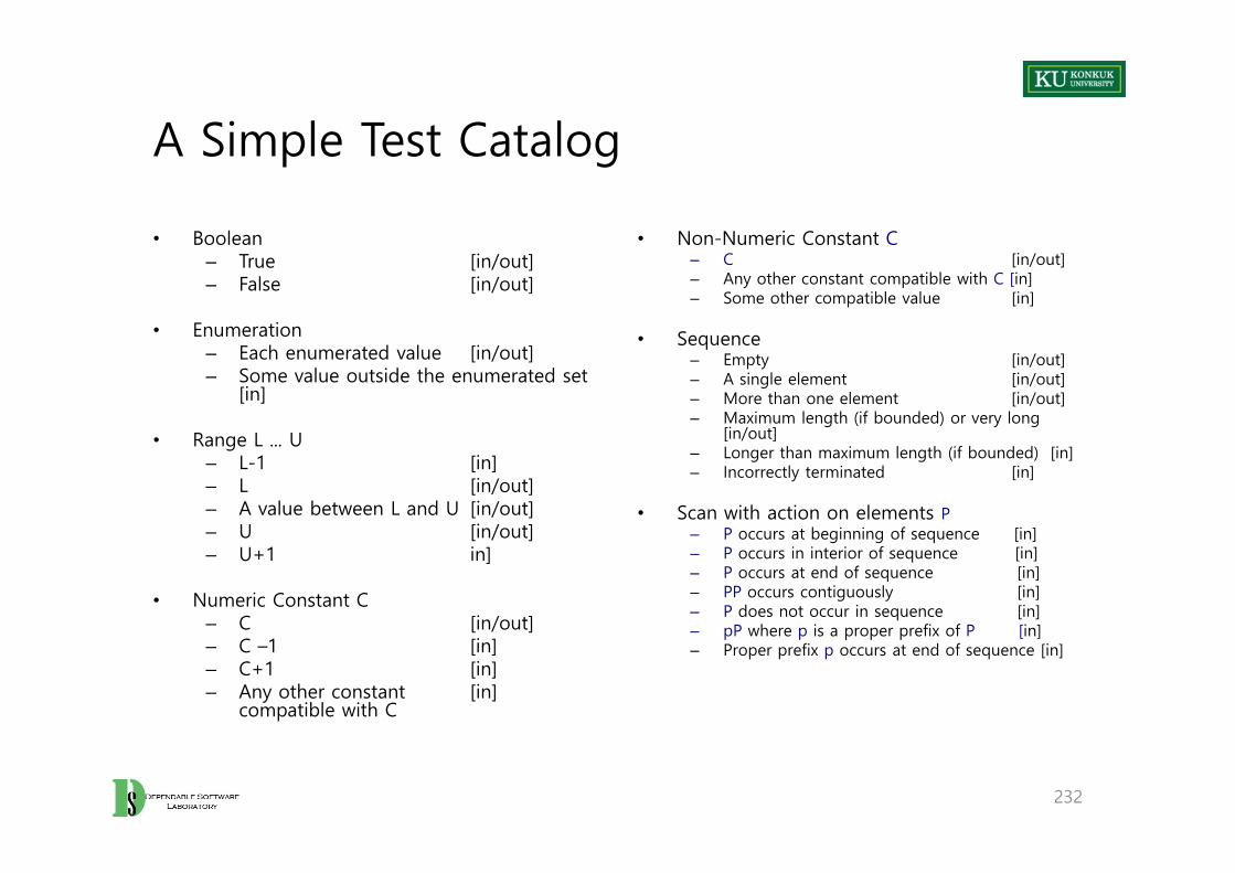
A Simple Test Catalog

• Boolean– True [in/out]– False [in/out]

• Enumeration– Each enumerated value [in/out]– Some value outside the enumerated set

[in]

• Range L ... U– L-1 [in]– L [in/out]– A value between L and U [in/out]– U [in/out]– U+1 in]

• Numeric Constant C– C [in/out]– C –1 [in]– C+1 [in]– Any other constant [in]

compatible with C

• Non-Numeric Constant C– C [in/out]– Any other constant compatible with C [in]– Some other compatible value [in]

• Sequence– Empty [in/out]– A single element [in/out]– More than one element [in/out]– Maximum length (if bounded) or very long

[in/out]– Longer than maximum length (if bounded) [in]– Incorrectly terminated [in]

• Scan with action on elements P– P occurs at beginning of sequence [in]– P occurs in interior of sequence [in]– P occurs at end of sequence [in]– PP occurs contiguously [in]– P does not occur in sequence [in]– pP where p is a proper prefix of P [in]– Proper prefix p occurs at end of sequence [in]

232

Catalog Entry: Boolean

• Boolean– True [in/out]– False [in/out]

• Application to return value generates 2 test cases already covered by TC-PRE2-1 and TC-PRE2-2.

233

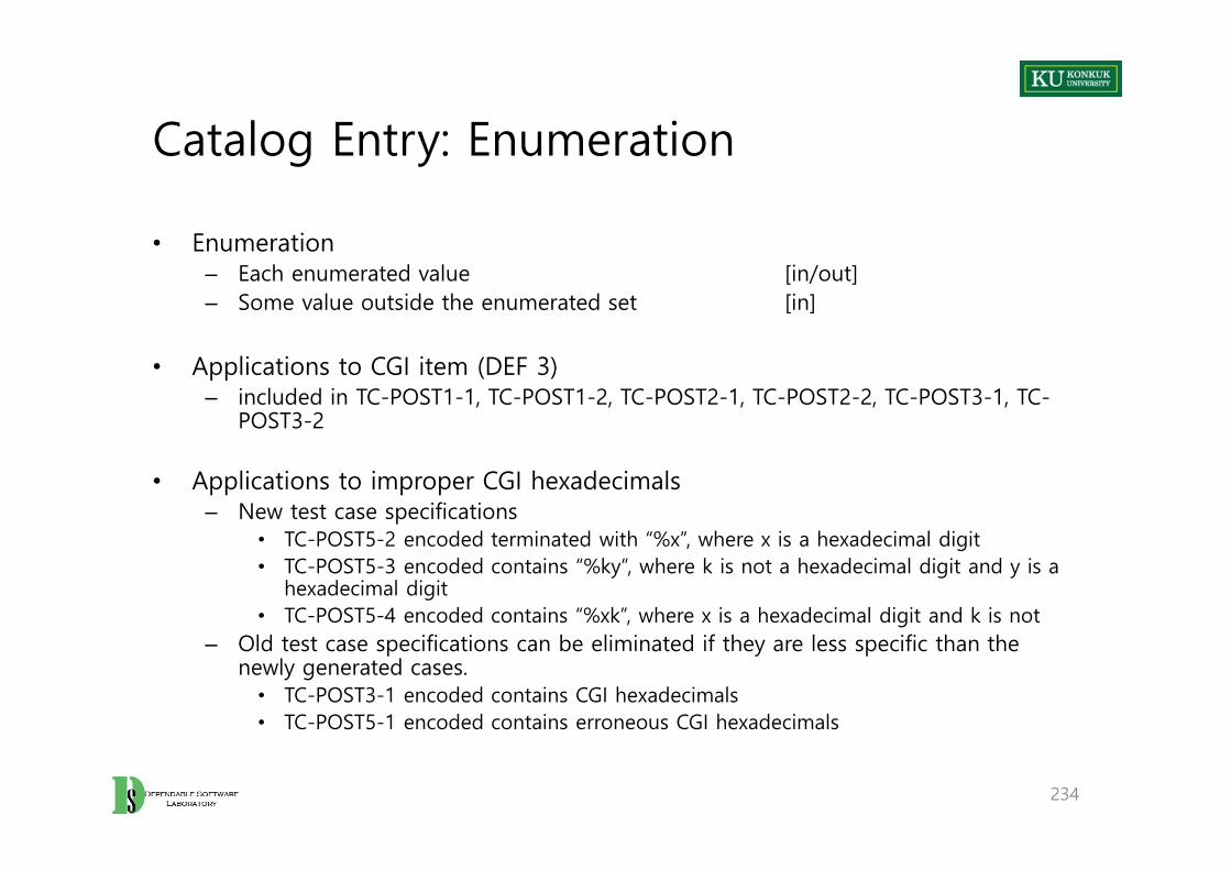
Catalog Entry: Enumeration

• Enumeration– Each enumerated value [in/out]– Some value outside the enumerated set [in]

• Applications to CGI item (DEF 3)– included in TC-POST1-1, TC-POST1-2, TC-POST2-1, TC-POST2-2, TC-POST3-1, TC-

POST3-2

• Applications to improper CGI hexadecimals– New test case specifications

• TC-POST5-2 encoded terminated with “%x”, where x is a hexadecimal digit• TC-POST5-3 encoded contains “%ky”, where k is not a hexadecimal digit and y is a

hexadecimal digit• TC-POST5-4 encoded contains “%xk”, where x is a hexadecimal digit and k is not

– Old test case specifications can be eliminated if they are less specific than the newly generated cases.

• TC-POST3-1 encoded contains CGI hexadecimals • TC-POST5-1 encoded contains erroneous CGI hexadecimals

234

Catalog Entries: the Others

We can apply in the same ways.

• range• numeric constant• non-numeric constant• sequence• scan

235

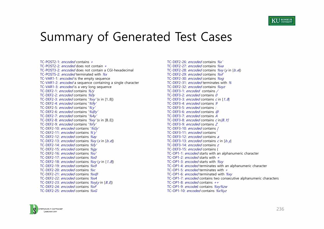
Summary of Generated Test Cases

TC-POST2-1: encoded contains + TC-POST2-2: encoded does not contain +TC-POST3-2: encoded does not contain a CGI-hexadecimal TC-POST5-2: encoded terminated with %xTC-VAR1-1: encoded is the empty sequenceTC-VAR1-2: encoded a sequence containing a single characterTC-VAR1-3: encoded is a very long sequenceTC-DEF2-1: encoded contains %/yTC-DEF2-2: encoded contains %0yTC-DEF2-3: encoded contains '%xy' (x in [1..8]) TC-DEF2-4: encoded contains '%9y'TC-DEF2-5: encoded contains '%:y'TC-DEF2-6: encoded contains '%@y‘TC-DEF2-7: encoded contains '%Ay' TC-DEF2-8: encoded contains '%xy' (x in [B..E])TC-DEF2-9: encoded contains '%Fy'TC-DEF2-10: encoded contains '%Gy‘TC-DEF2-11: encoded contains %`y'TC-DEF2-12: encoded contains %ayTC-DEF2-13: encoded contains %xy (x in [b..e]) TC-DEF2-14: encoded contains %fy'TC-DEF2-15: encoded contains %gyTC-DEF2-16: encoded contains %x/TC-DEF2-17: encoded contains %x0TC-DEF2-18: encoded contains %xy (y in [1..8])TC-DEF2-19: encoded contains %x9TC-DEF2-20: encoded contains %x:TC-DEF2-21: encoded contains %x@TC-DEF2-22: encoded contains %xATC-DEF2-23: encoded contains %xy(y in [B..E])TC-DEF2-24: encoded contains %xFTC-DEF2-25: encoded contains %xG

TC-DEF2-26: encoded contains %x`TC-DEF2-27: encoded contains %xaTC-DEF2-28: encoded contains %xy (y in [b..e])TC-DEF2-29: encoded contains %xfTC-DEF2-30: encoded contains %xgTC-DEF2-31: encoded terminates with %TC-DEF2-32: encoded contains %xyzTC-DEF3-1: encoded contains /TC-DEF3-2: encoded contains 0TC-DEF3-3: encoded contains c in [1..8]TC-DEF3-4: encoded contains 9TC-DEF3-5: encoded contains :TC-DEF3-6: encoded contains @TC-DEF3-7: encoded contains ATC-DEF3-8: encoded contains c in[B..Y]TC-DEF3-9: encoded contains ZTC-DEF3-10: encoded contains [TC-DEF3-11: encoded contains`TC-DEF3-12: encoded contains aTC-DEF3-13: encoded contains c in [b..y]TC-DEF3-14: encoded contains zTC-DEF3-15: encoded contains {TC-OP1-1: encoded starts with an alphanumeric characterTC-OP1-2: encoded starts with +TC-OP1-3: encoded starts with %xyTC-OP1-4: encoded terminates with an alphanumeric characterTC-OP1-5: encoded terminates with +TC-OP1-6: encoded terminated with %xyTC-OP1-7: encoded contains two consecutive alphanumeric charactersTC-OP1-8: encoded contains ++TC-OP1-9: encoded contains %xy%zwTC-OP1-10: encoded contains %x%yz

236

What Have We Got from Three Methods?

• From category partition testing: – Division into a (manual) step of identifying categories and values, with

constraints, and an (automated) step of generating combinations

• From catalog-based testing: – Improving the manual step by recording and using standard patterns for

identifying significant values

• From pairwise testing: – Systematic generation of smaller test suites

• Three ideas can be combined.

237

Summary

• Requirements specifications typically begin in the form of natural language statements.

– But, flexibility and expressiveness of natural language is an obstacle to automatic analysis.

• Combinatorial approaches to functional testing consist of – A manual step of structuring specifications into set of properties – An automatic(-able) step of producing combinations of choices

• Brute force synthesis of test cases is tedious and error prone.– Combinatorial approaches decompose brute force work into steps to attack

the problem incrementally by separating analysis and synthesis activities that can be quantified and monitored, and partially supported by tools.

238

239

Chapter 12. Structural Testing

Learning Objectives

• Understand rationale for structural testing – How structural testing complements functional testing

• Recognize and distinguish basic terms such as adequacy and coverage• Recognize and distinguish characteristics of common structural criteria• Understand practical uses and limitations of structural testing

241

Structural Testing

• Judging test suite thoroughness based on the structure of the programitself

– Also known as • White-box testing• Glass-box testing • Code-based testing

– Distinguish from functional (requirements-based, “black-box”) testing

• Structural testing is still testing product functionality against its specification.

– Only the measure of thoroughness has changed.

242

Rationale of Structural Testing

• One way of answering the question “What is missing in our test suite?”– If a part of a program is not executed by any test case in the suite, faults in

that part cannot be exposed.– But what’s the ‘part’?

• Typically, a control flow element or combination• Statements (or CFG nodes), Branches (or CFG edges)• Fragments and combinations: Conditions, paths

• Structural testing complements functional testing.– Another way to recognize cases that are treated differently

• Recalling fundamental rationale– Prefer test cases that are treated differently over cases treated the same

243

No Guarantee

• Executing all control flow elements does not guarantee finding all faults.– Execution of a faulty statement may not always result in a failure.

• The state may not be corrupted when the statement is executed with some data values.

• Corrupt state may not propagate through execution to eventually lead to failure.

• What is the value of structural coverage?– Increases confidence in thoroughness of testing

244

Structural Testing Complements Functional Testing

• Control flow-based testing includes cases that may not be identified from specifications alone.

– Typical case: Implementation of a single item of the specification by multiple parts of the program

– E.g. Hash table collision (invisible in interface specification)

• Test suites that satisfy control flow adequacy criteria could fail in revealing faults that can be caught with functional criteria.

– Typical case: Missing path faults

245

Structural Testing, in Practice

• Create functional test suite first, then measure structural coverage to identify and see what is missing.

• Interpret unexecuted elements– May be due to natural differences between specification and implementation– May reveal flaws of the software or its development process

• Inadequacy of specifications that do not include cases present in the implementation

• Coding practice that radically diverges from the specification• Inadequate functional test suites

• Attractive because structural testing is automated– Coverage measurements are convenient progress indicators.– Sometimes used as a criterion of completion of testing

• Use with caution: does not ensure effective test suites

246

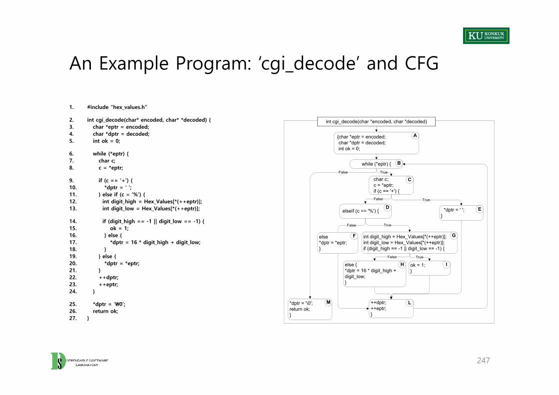
An Example Program: ‘cgi_decode’ and CFG

1. #include “hex_values.h”

2. int cgi_decode(char* encoded, char* *decoded) {3. char *eptr = encoded;4. char *dptr = decoded;5. int ok = 0;

6. while (*eptr) {7. char c;8. c = *eptr;

9. if (c == ‘+’) {10. *dptr = ‘ ‘;11. } else if (c = ‘%’) {12. int digit_high = Hex_Values[*(++eptr)];13. int digit_low = Hex_Values[*(++eptr)];

14. if (digit_high == -1 || digit_low == -1) {15. ok = 1;16. } else {17. *dptr = 16 * digit_high + digit_low;18. }19. } else {20. *dptr = *eptr;21. }22. ++dptr;23. ++eptr;24. }

25. *dptr = ‘\0’;26. return ok;27. }

247

{char *eptr = encoded;char *dptr = decoded;int ok = 0;

char c;c = *eptr;if (c == '+') {

*dptr = ' ';}

while (*eptr) {True

*dptr = '\0';return ok;}

False

True

int digit_high = Hex_Values[*(++eptr)];int digit_low = Hex_Values[*(++eptr)];if (digit_high == -1 || digit_low == -1) {

True

ok = 1;}

True

else {*dptr = 16 * digit_high + digit_low;}

False

++dptr;++eptr;}

False

False

elseif (c == '%') {

else*dptr = *eptr;}

int cgi_decode(char *encoded, char *decoded)

A

C

B

D E

F G

H I

LM

Structural Testing Techniques

1. Statement Testing

2. Branch Testing

3. Condition Testing– Basic– Compounded– MC/DC

4. Path Testing– Bounded interior– Loop boundary– LCSAJ– Cyclomatic

248

1. Statement Testing

• Adequacy criterion: – Each statement (or node in the CFG) must be executed at least once.

• Coverage:number of executed statements

number of statements

• Rationale: – A fault in a statement can only be revealed by executing the faulty statement.

• Nodes in a CFG often represent basic blocks of multiple statements.– Some standards refer to ‘basic block coverage’ or ‘node coverage’.– Difference in granularity, but not in concept

249

An Example: for Function “cgi_decode”

250

< Test cases >T0 = {“”, “test”, “test+case%1Dadequacy”}17/18 = 94% Statement coverage

T1 = {“adequate+test%0Dexecution%7U”}18/18 = 100% Statement coverage

T2 = {“%3D”, “%A”, “a+b”, “test”}18/18 = 100% Statement coverage

T3 = {“ ”, “+%0D+%4J”}…

T4 = {“first+test%9Ktest%K9”}…

Coverage is not a Matter of Size

• Coverage does not depend on the number of test cases.– T0 , T1 : T1 >coverage T0 T1 <cardinality T0

– T1 , T2 : T2 =coverage T1 T2 >cardinality T1

• Minimizing test suite size is not the goal.– Small test cases make failure diagnosis easier.– But, a failing test case in T2 gives more information for fault localization than

a failing test case in T1

251

Complete Statement Coverage

• Complete statement coverage may not imply executing all branches in a program.

• Example: – Suppose block F were missing– But, statement adequacy would

not require false branch from D to L

• T3 = {“ ”, “+%0D+%4J”}– 100% statement coverage– No false branch from D

252

{char *eptr = encoded;char *dptr = decoded;int ok = 0;

char c;c = *eptr;if (c == '+') {

*dptr = ' ';}

while (*eptr) {True

*dptr = '\0';return ok;}

False

True

int digit_high = Hex_Values[*(++eptr)];int digit_low = Hex_Values[*(++eptr)];if (digit_high == -1 || digit_low == -1) {

True

ok = 1;}

True

else {*dptr = 16 * digit_high + digit_low;}

False

++dptr;++eptr;}

False

False

elseif (c == '%') {

else {*dptr = *eptr;}

int cgi_decode(char *encoded, char *decoded)

A

C

B

D E

F G

H I

LM

2. Branch Testing

• Adequacy criterion: – Each branch (edge in the CFG) must be executed at least once.

• Coverage:number of executed branches

number of branches

• Example:– T3 = {“”, “+%0D+%4J”}

• 100% Stmt Cov.• 88% Branch Cov. (7/8 branches)

– T2 = {“%3D”, “%A”, “a+b”, “test”}• 100% Stmt Cov. • 100% Branch Cov. (8/8 branches)

253

Statements vs. Branches

• Traversing all edges causes all nodes to be visited.– Therefore, test suites that satisfy the branch adequacy also satisfy the

statement adequacy criterion for the same program.– Branch adequacy subsumes statement adequacy.

• The converse is not true (see T3)– A statement-adequate test suite may not be branch-adequate.

254

All Branches Coverage

• “All branches coverage” can still miss conditions.

• Example: – Supposed that we missed the negation operator of “digit_high == -1”

digit_high == 1 || digit_low == -1

• Branch adequacy criterion can be satisfied by varying only ‘digit_low’.– The faulty sub-expression might never determine the result.– We might never really test the faulty condition, even though we tested both

outcomes of the branch.

255

3. Condition Testing

• Branch coverage exposes faults in how a computation has been decomposed into cases.

– Intuitively attractive: checking the programmer’s case analysis– But, only roughly: grouping cases with the same outcome

• Condition coverage considers case analysis in more detail.– Consider ‘individual conditions’ in a compound Boolean expression

• E.g. both parts of ‘”igit_high == 1 || digit_low == -1”

• Adequacy criterion: – Each basic condition must be executed at least once.

• Basic condition testing coverage:number of truth values taken by all basic conditions

2 * number of basic conditions

256

Basic Conditions vs. Branches

• Basic condition adequacy criterion can be satisfied without satisfying branch coverage.

• T4 = {“first+test%9Ktest%K9”}– Satisfies basic condition adequacy– But, does not satisfy branch condition adequacy

• Branch and basic condition are not comparable. – Neither implies the other.

257

Covering Branches and Conditions

• Branch and condition adequacy: – Cover all conditions and all decisions

• Compound condition adequacy:– Cover all possible evaluations of compound conditions.– Cover all branches of a decision tree.

258

truefalse

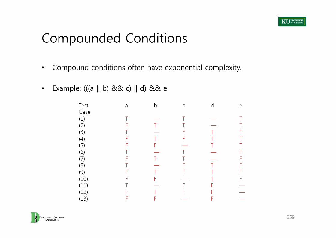
Compounded Conditions

• Compound conditions often have exponential complexity.

• Example: (((a || b) && c) || d) && e

259

Modified Condition/Decision (MC/DC)

• Motivation– Effectively test important combinations of conditions, without exponential

blowup in test suite size – “Important” combinations means:

• Each basic condition shown to independently affect the outcome of each decision

• Requires– For each basic condition C, two test cases,– Values of all ‘evaluated’ conditions except C are the same.– Compound condition as a whole evaluates to ‘true’ for one and ‘false’ for the

other.

260

Complexity of MC/DC

• MC/DC has a linear complexity.

• Example: (((a || b) && c) || d) && e

Test a b c d e outcomeCase(1) true -- true -- true true(2) false true true -- true true(3) true -- false true true true(6) true -- true -- false false(11) true -- false false -- false(13) false false -- false -- false

• Underlined values independently affect the output of the decision.– Required by the RTCA/DO-178B standard

261

Comments on MC/DC

• MC/DC is – Basic condition coverage (C)– Branch coverage (DC)– Plus one additional condition (M)

• Every condition must independently affect the decision’s output.

• It is subsumed by compound conditions and subsumes all other criteria discussed so far.

– Stronger than statement and branch coverage

• A good balance of thoroughness and test size – Widely used

262

4. Path Testing

• There are many more paths than branches.– Decision and condition adequacy criteria consider individual decisions only.

• Path testing focuses combinations of decisions along paths.

• Adequacy criterion: – Each path must be executed at least once.

• Coverage:number of executed paths

number of paths

263

Path Coverage Criteria in Practice

• The number of paths in a program with loops is unbounded. – Usually impossible to satisfy

• For a feasible criterion, – Should partition infinite set of paths into a finite number of classes

• Useful criteria can be obtained by limiting – Number of traversals of loops– Length of the paths to be traversed– Dependencies among selected paths

264

Boundary Interior Path Testing

• Group together paths that differ only in the subpath they follow, when repeating the body of a loop

– Follow each path in the CFG up to the first repeated node– The set of paths from the root of the tree to each leaf is the required set of

subpaths for boundary interior coverage.

265Paths for boundary interior path testingPaths derived from the CFG

Limitations of Boundary Interior Adequacy

• The number of paths can still grow exponentially

266

if (a) { S1; }if (b) { S2; }if (c) { S3; }...if (x) { Sn; }

• The subpaths through this control flow can include or exclude each of the statements Si, so that in total N branches result in 2N paths that must be traversed.

• Choosing input data to force execution of one particular path may be very difficult, or even impossible if the conditions are not independent.

Loop Boundary Adequacy

• Variant of the boundary/interior criterion– Treats loop boundaries similarly, but is less stringent with respect to other

differences among paths.

• Criterion: – A test suite satisfies the loop boundary adequacy criterion iff, for every loop:

• In at least one test case, the loop body is iterated zero times.• In at least one test case, the loop body is iterated once.• In at least one test case, the loop body is iterated more than once.

• Corresponds to the cases that would be considered in a formal correctness proof for the loop

267

LCSAJ Adequacy

• Linear Code Sequence And Jumps (LCSAJ)– Sequential subpath in the CFG starting and ending in a branch

• TER1 = statement coverage• TER2 = branch coverage• TERn+2 = coverage of n consecutive LCSAJs

– Essentially considering full path coverage of (short) sequences of decisions

• Data flow criteria considered in a later chapter provide a more principled way of choosing some particular sub-paths as important enough to cover in testing.

– But, neither LCSAJ nor data flow criteria are much used in current practice.

268

Cyclomatic Adequacy

269

• Cyclomatic number– Number of independent paths in the CFG– A path is representable as a bit vector, where each component of the vector

represents an edge.– “Dependence” is ordinary linear dependence between (bit) vectors

• If e = #edges, n = #nodes, c = #connected components of a graph, – e - n + c for an arbitrary graph– e - n + 2 for a CFG ← Cyclomatic complexity

• Cyclomatic coverage counts the number of independent paths that have been exercised, relative to cyclomatic complexity.

Procedure Call Testing

• Measure coverage of control flow within individual procedures. – Not well suited to integration or system testing

• Choose a coverage granularity commensurate with the granularity of testing

– If unit testing has been effective, then faults that remain to be found in integration testing will be primarily interface faults, and testing effort should focus on interfaces between units rather than their internal details.

• Procedure entry and exit testing– Procedure may have multiple entry points (e.g., Fortran) and multiple exit

points.

• Call coverage– The same entry point may be called from many points.

270

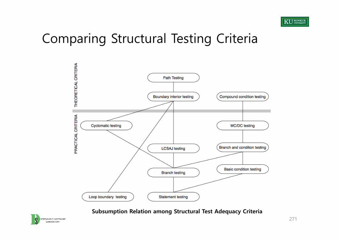
Comparing Structural Testing Criteria

271

Subsumption Relation among Structural Test Adequacy Criteria

The Infeasibility Problem

• Sometimes criteria may not be satisfiable.– The criterion requires execution of

• Statements that cannot be executed as a result of – Defensive programming – Code reuse (reusing code that is more general than strictly required for the

application)

• Conditions that cannot be satisfied as a result of – Interdependent conditions

• Paths that cannot be executed as a result of – Interdependent decisions

272

Satisfying Structural Criteria

• Large amounts of ‘fossil’ code may indicate serious maintainability problems.

• But, some unreachable code is common even in well-designed and well-maintained systems.

• Solutions:1. Make allowances by setting a coverage goal less than 100%2. Require justification of elements left uncovered

• As RTCA-DO-178B and EUROCAE ED-12B for modified MC/DC

273

Summary

• We defined a number of adequacy criteria. – NOT test design techniques– Different criteria address different classes of errors.

• Full coverage is usually unattainable.– Attainability is an undecidable problem.

• Rather than requiring full adequacy, the “degree of adequacy” of a test suite is estimated by coverage measures.

274

275

Chapter 13. Data Flow Testing

Learning Objectives

• Understand why data flow criteria have been designed and used• Recognize and distinguish basic DF criteria

– All DU pairs, all DU paths, all definitions

• Understand how the infeasibility problem impacts data flow testing• Appreciate limits and potential practical uses of data flow testing

277

Motivation

• Middle ground in structural testing– Node and edge coverage don’t test interactions.– Path-based criteria require impractical number of test cases.

• Only a few paths uncover additional faults, anyway.

– Need to distinguish “important” paths

• Intuition: Statements interact through data flow.– Value computed in one statement, is used in another.– Bad value computation can be revealed only when it is used.

278

Def-Use Pairs

• Value of x at 6 could be computed at 1 or at 4.

• Bad computation at 1 or 4 could be revealed only if they are used at 6.

• (1, 6) and (4, 6) are def-use (DU) pairs.

– defs at 1, 4– use at 6

279

x = ....

if ....

x = ....

...

....

y = x + ...

4

1

6

2

3

5

Terminology

• DU pair– A pair of definition and use for some variable, such that at least one DU path

exists from the definition to the use.– “x = ...” is a definition of x– “= ... x ...” is a use of x

• DU path – A definition-clear path on the CFG starting from a definition to a use of a

same variable– Definition clear: Value is not replaced on path.– Note: Loops could create infinite DU paths between a def and a use.

280

Definition-Clear Path

• 1,2,3,5,6 is a definition-clear path from 1 to 6.

– x is not re-assigned between 1 and 6.

• 1,2,4,5,6 is not a definition-clear path from 1 to 6.

– the value of x is “killed” (reassigned) at node 4.

• (1, 6) is a DU pair because 1,2,3,5,6 is a definition-clear path.

281

x = ....

if ....

x = ....

...

....

y = x + ...

4

1

6

2

3

5

Adequacy Criteria

• All DU pairs – Each DU pair is exercised by at least one test case.

• All DU paths – Each simple (non looping) DU path is exercised by at least one test case.

• All definitions– For each definition, there is at least one test case which exercises a DU pair

containing it.– Because, every computed value is used somewhere.

• Corresponding coverage fractions can be defined similarly.

282

Difficult Cases

• x[i] = ... ; ... ; y = x[ j]– DU pair (only) if i==j

• p = &x ; ... ; *p = 99 ; ... ; q = x– *p is an alias of x

• m.putFoo(...); ... ; y=n.getFoo(...); – Are m and n the same object?– Do m and n share a “foo” field?

• Problem of aliases: – Which references are (always or sometimes) the same?

283

Data Flow Coverage with Complex Structures

• Arrays and pointers are critical for data flow analysis.– Under-estimation of aliases may fail to include some DU pairs.– Over-estimation may introduce unfeasible test obligations.

• For testing, it may be preferable to accept under-estimation of alias set rather than over-estimation or expensive analysis.

– Alias analysis may rely on external guidance or other global analysis to calculate good estimates.

– Undisciplined use of dynamic storage, pointer arithmetic, etc. may make the whole analysis infeasible.

– But, in other applications (e.g., compilers), a conservative over-estimation of aliases is usually required.

284

The Infeasibility Problem

• Suppose ‘cond’ has not changed between 1 and 5.

– Or the conditions could be different, but the first implies the second.

• Then (3,5) is not a (feasible) DU pair.

– But it is difficult or impossible to determine which pairs are infeasible.

• Infeasible test obligations are a problem.

– No test case can cover them.

285

Why? – I don’t Know!

if (cond)

x = ....

...

....

y = x + ...

3

1

2

4

if (cond)

.... 6

5

7

Data Flow Coverage in Practice

• The path-oriented nature of data flow analysis makes the infeasibility problem especially relevant.

– Combinations of elements matter.– Impossible to (infallibly) distinguish feasible from infeasible paths. – More paths = More work to check manually

• In practice, reasonable coverage is (often, not always) achievable.– Number of paths is exponential in worst case, but often linear.– All DU paths is more often impractical.

286

Summary

• Data flow testing attempts to distinguish “important” paths: Interactions between statements.

– Intermediate between simple statement and branch coverage and more expensive path-based structural testing

• Cover Def-Use (DU) pairs: From computation of value to its use– Intuition: Bad computed value is revealed only when it is used.– Levels: All DU pairs, all DU paths, all defs (some use)

• Limits: Aliases, infeasible paths– Worst case is bad (undecidable properties, exponential blowup of paths), so

pragmatic compromises are required.

287

288

Chapter 14. Model-Based Testing

Learning Objectives

• Understand the role of models in devising test cases– Principles underlying functional and structural test adequacy criteria, as well

as model-based testing

• Understand some examples of model-based testing techniques• Be able to understand, devise and refine other model-based testing

techniques

290

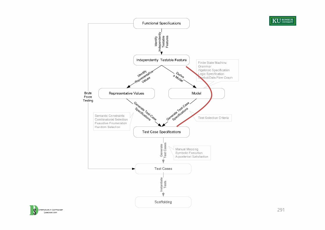
291

Iden

tify

Inde

pend

ently

Te

stab

le

Feat

ures

Generate Test-Case

Specifications Generate Test-Case

Specifications

Gen

erat

e Te

st C

ases

Inst

antia

teTe

sts

Overview

• Models used in specification or design have structure.– Useful information for selecting representative classes of behavior – Behaviors that are treated differently with respect to the model should be

tried by a thorough test suite.– In combinatorial testing, it is difficult to capture that structure clearly and

correctly in constraints.

• We can devise test cases to check actual behavior against behavior specified by the model.

– “Coverage” similar to structural testing, but applied to specification and design models

292

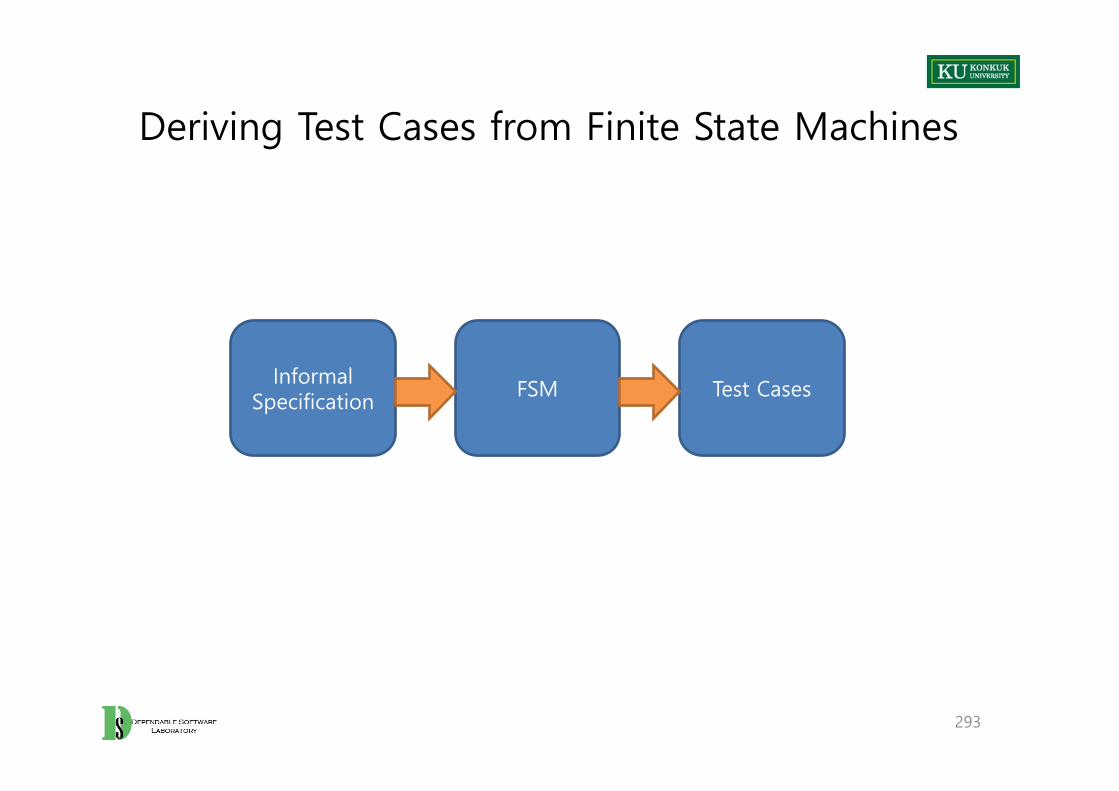
Deriving Test Cases from Finite State Machines

293

Informal Specification

FSM Test Cases

Informal Specification: Feature “Maintenance” of the Chipmunk Web Site

Maintenance: The Maintenance function records the history of items undergoing maintenance.

If the product is covered by warranty or maintenance contract, maintenance can be requested either by calling the maintenance toll free number, or through the web site, or by bringing the item to a designated maintenance station.If the maintenance is requested by phone or web site and the customer is a US or EU resident, the item is picked up at the customer site, otherwise, the customer shall ship the item with an express courier.If the maintenance contract number provided by the customer is not valid, the item follows the procedure for items not covered by warranty.If the product is not covered by warranty or maintenance contract, maintenance can be requested only by bringing the item to a maintenance station. The maintenance station informs the customer of the estimated costs for repair. Maintenance starts only when the customer accepts the estimate. If the customer does not accept the estimate, the product is returned to the customer.Small problems can be repaired directly at the maintenance station. If the maintenance station cannot solve the problem, the product is sent to the maintenance regional headquarters (if in US or EU) or to the maintenance main headquarters (otherwise).If the maintenance regional headquarters cannot solve the problem, the product is sent to the maintenance main headquarters.Maintenance is suspended if some components are not available.Once repaired, the product is returned to the customer.

294

Corresponding Finite State Machine

295

NO Maintenance

Maintenance(no warranty)

estim

ate

cost

s

request at

maintenance station

(no warranty)

request by phone or web

[US or EU resident]

(contract number)

Wait forpick up

Repair(maintenance

station)

pick up

requ

est a

t m

aint

enan

ce s

tatio

nor

by

expr

ess

cour

ier

(con

tract

num

ber)

Wait for acceptance

acceptestimate

Wait for returning

reject estimate

pick up

Repairedrepair completed

return

Repair(regional

headquarters)

Repair(main

headquarters)

successf

ul repair

unable to repair

(US or EU resident)

succ

essfu

l rep

air

unable to repair

Wait for component

lack co

mponent (a)

lack component (b)

lack component (c)componentarrives (c)

componentarrives (b)

componentarrives (a)

invalidcontractnumber

unable to repair(not US or EU resident)

1 2 3

0

4 5 6

7 8

9

Test Cases Generated from the FSM

• FSM can be used both to1. Guide test selection (checking each state transition)2. Constructing an oracle that judge whether each observed behavior is correct

• Questions:– Is this a thorough test suite? – How can we judge? Coverage criteria require.

296

TC1 0 2 4 1 0

TC2 0 5 2 4 5 6 0

TC3 0 3 5 9 6 0

TC4 0 3 5 7 5 8 7 8 9 6 0

Transition Coverage Criteria

• State coverage– Every state in the model should be visited by at least one test case.

• Transition coverage– Every transition between states should be traversed by at least one test case. – Most commonly used criterion– A transition can be thought of as a (precondition, postcondition) pair

297

Path Sensitive Criteria

• Basic assumption: States fully summarize history.– No distinction based on how we reached a state – But, this should be true of well-designed state machine models.

• If the assumption is violated, we may distinguish paths and devise criteria to cover them

– Single state path coverage: • Traverse each subpath that reaches each state at most once

– Single transition path coverage: • Traverse each subpath that reaches each transition at most once

– Boundary interior loop coverage: • Each distinct loop of the state machine must be exercised the minimum, an

intermediate, and the maximum or a large number of times• Of the path sensitive criteria, only boundary-interior is common.

298

Deriving Test Cases from Decision Structures

• Some specifications are structured as decision tables, decision trees, or flow charts.

• We can exercise these as if they were program source code.

299

Informal Specification

Decision Structures

Test Cases

Informal Specification: Feature “Price” of the Chipmunk Web Site

Pricing: The pricing function determines the adjusted price of a configuration for a particular customer.

The scheduled price of a configuration is the sum of the scheduled price of the model and the scheduled price of each component in the configuration. The adjusted price is either the scheduled price, if no discounts are applicable, or the scheduled price less any applicable discounts.There are three price schedules and three corresponding discount schedules, Business, Educational, and Individual.….

Educational prices: The adjusted price for a purchase charged to an educational account in good standing is the scheduled price from the educational price schedule. No further discounts apply.…

Special-price non-discountable offers: Sometimes a complete configuration is offered at a special, non-discountable price. When a special, non-discountable price is available for a configuration, the adjusted price is the non-discountable price or the regular price after any applicable discounts, whichever is less.

300

Corresponding Decision Table

Education Individual

EduAc T T F F F F F F

BusAc - - F F F F F F

CP > CT1 - - F F T T - -

YP > YT1 - - - - - - - -

CP > CT2 - - - - F F T T

YP > YT2 - - - - - - - -

SP < Sc F T F T - - - -

SP < T1 - - - - F T - -

SP < T2 - - - - - - F T

Out Edu SP ND SP T1 SP T2 SP

301

…

Constraintsat-most-one (EduAc, BusAc) at-most-one (YP < YT1, YP > YT2) YP > YT2 → YP > YT1 at-most-one (CP < CT1, CP > CT2)CP > CT2 → CP > CT1 at-most-one (SP < T1, SP > T2SP > T2 → SP > T1

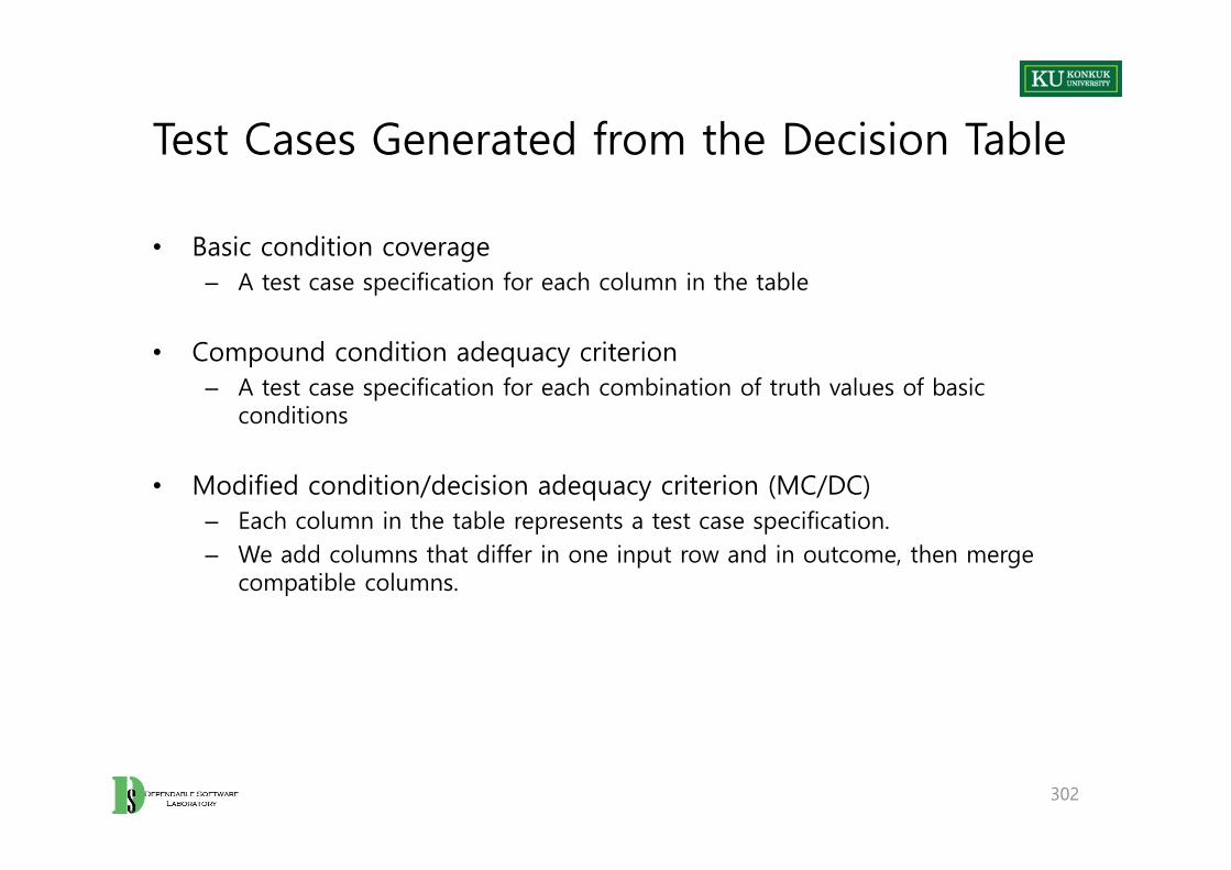
Test Cases Generated from the Decision Table

• Basic condition coverage– A test case specification for each column in the table

• Compound condition adequacy criterion– A test case specification for each combination of truth values of basic

conditions

• Modified condition/decision adequacy criterion (MC/DC)– Each column in the table represents a test case specification.– We add columns that differ in one input row and in outcome, then merge

compatible columns.

302

A Part of Test Cases by Applying MC/DC

303

C.1 C.1a C.1b C.10

EduAc T F T -

BusAc - - - T

CP > CT1 - - - F

YP > YT1 - - - F

CP > CT2 - - - -

YP > YT2 - - - -

SP > Sc F F T T

SP > T1 - - - -

SP > T2 - - - -

Out Edu * * SP

Generate C.1a and C.1b by flipping one

element of C.1.

C.1b can be merged with an existing

column (C.10) in the specification. (?)

Outcome of generated columns must differ from source column

Deriving Test Cases from Control and Data Flow Graph

• If the specification or model has both decisions and sequential logic, we can cover it like program source code.

• Flowgraph based testing

304

Informal Specification

Flowgraph Test Cases

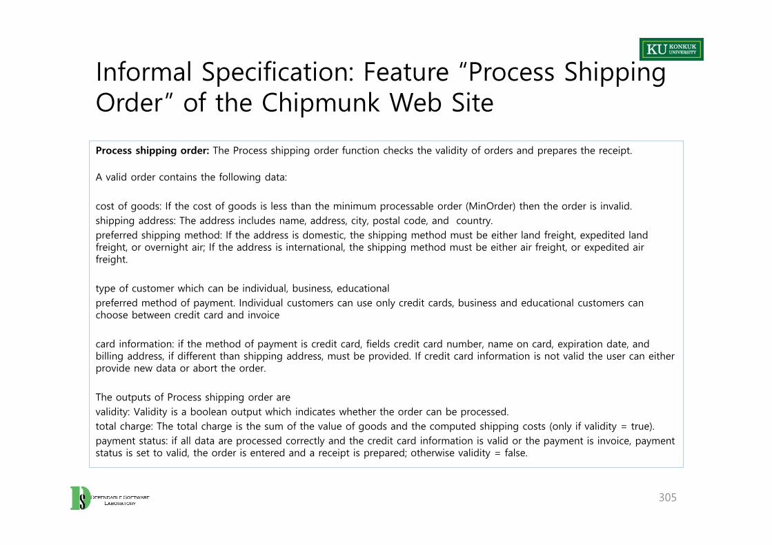
Informal Specification: Feature “Process Shipping Order” of the Chipmunk Web Site

Process shipping order: The Process shipping order function checks the validity of orders and prepares the receipt.

A valid order contains the following data:

cost of goods: If the cost of goods is less than the minimum processable order (MinOrder) then the order is invalid.shipping address: The address includes name, address, city, postal code, and country.preferred shipping method: If the address is domestic, the shipping method must be either land freight, expedited land freight, or overnight air; If the address is international, the shipping method must be either air freight, or expedited air freight.

type of customer which can be individual, business, educationalpreferred method of payment. Individual customers can use only credit cards, business and educational customers can choose between credit card and invoice

card information: if the method of payment is credit card, fields credit card number, name on card, expiration date, and billing address, if different than shipping address, must be provided. If credit card information is not valid the user can either provide new data or abort the order.

The outputs of Process shipping order arevalidity: Validity is a boolean output which indicates whether the order can be processed.total charge: The total charge is the sum of the value of goods and the computed shipping costs (only if validity = true). payment status: if all data are processed correctly and the credit card information is valid or the payment is invoice, payment status is set to valid, the order is entered and a receipt is prepared; otherwise validity = false.

305

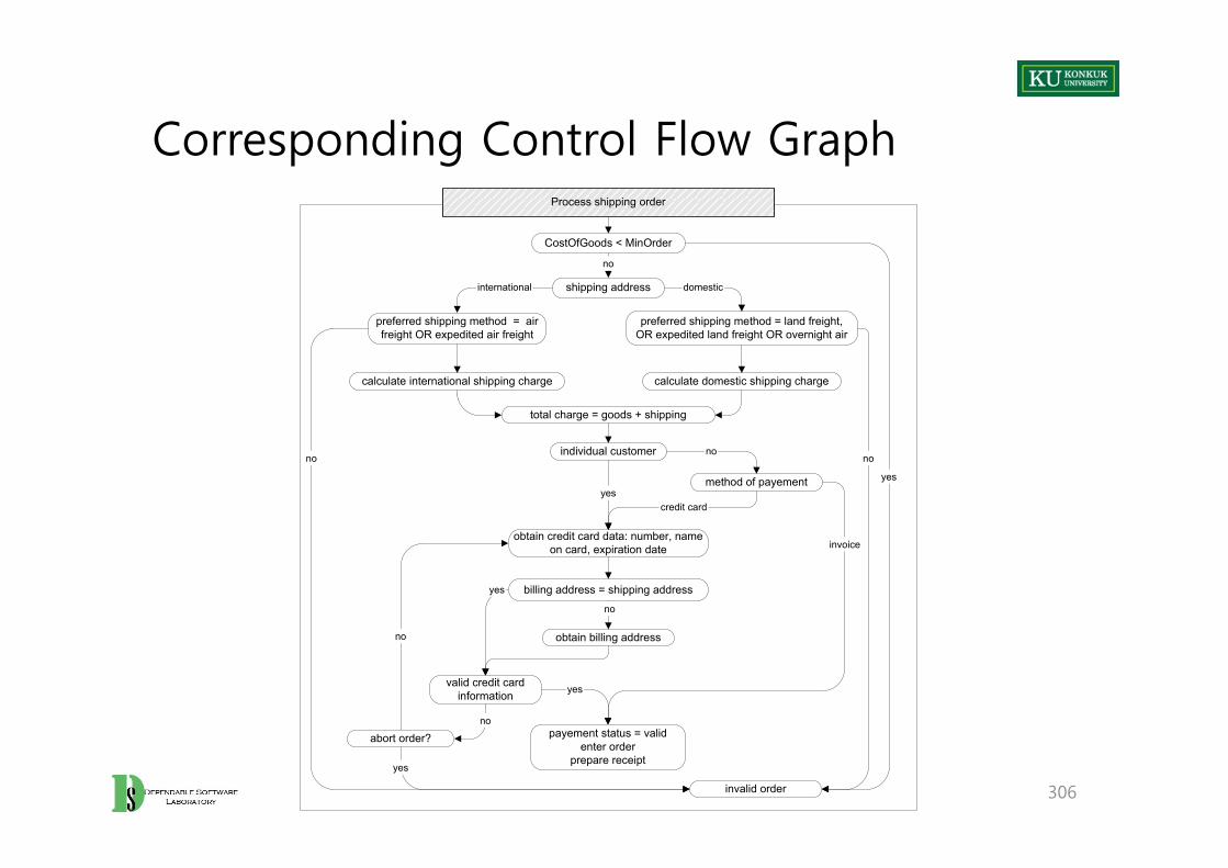
Corresponding Control Flow Graph

306

preferred shipping method = land freight,OR expedited land freight OR overnight air

Process shipping order

CostOfGoods < MinOrder

shipping address

no

yes

domestic

preferred shipping method = airfreight OR expedited air freight

international

calculate domestic shipping chargecalculate international shipping charge

total charge = goods + shipping

individual customer no

yes

obtain credit card data: number, nameon card, expiration date

method of payement

credit card

invoice

billing address = shipping address

obtain billing address

no

yes

valid credit cardinformation

no

yes

payement status = validenter order

prepare receipt

invalid order

nono

abort order?no

yes

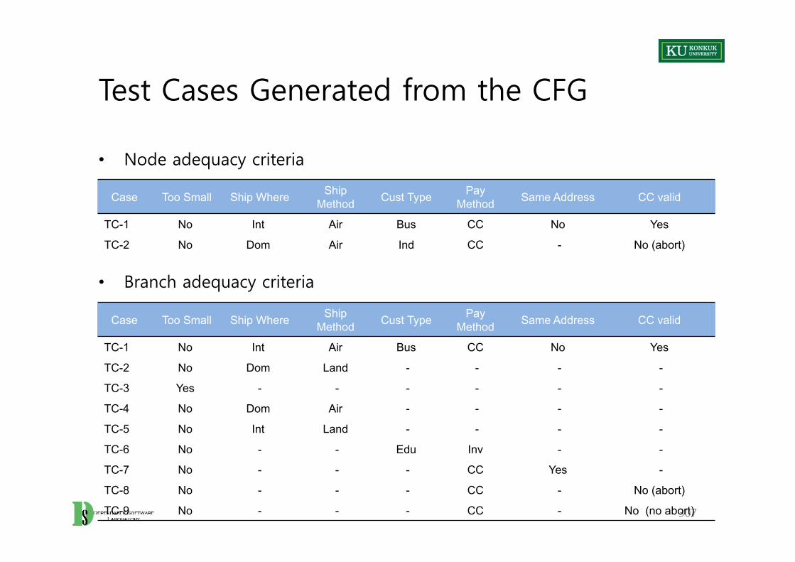
Test Cases Generated from the CFG

• Node adequacy criteria

• Branch adequacy criteria

307

Case Too Small Ship Where Ship Method Cust Type Pay

Method Same Address CC valid

TC-1 No Int Air Bus CC No Yes

TC-2 No Dom Land - - - -

TC-3 Yes - - - - - -

TC-4 No Dom Air - - - -

TC-5 No Int Land - - - -

TC-6 No - - Edu Inv - -

TC-7 No - - - CC Yes -

TC-8 No - - - CC - No (abort)

TC-9 No - - - CC - No (no abort)

Case Too Small Ship Where Ship Method Cust Type Pay

Method Same Address CC valid

TC-1 No Int Air Bus CC No Yes

TC-2 No Dom Air Ind CC - No (abort)

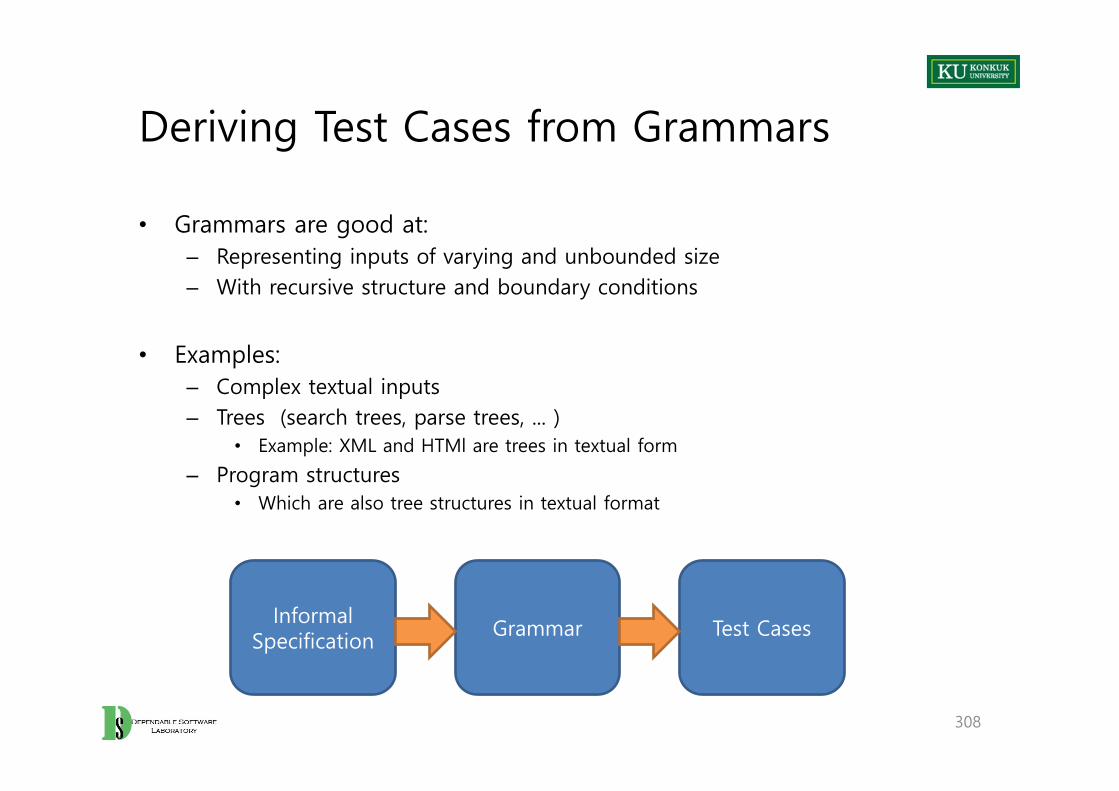
Deriving Test Cases from Grammars

• Grammars are good at:– Representing inputs of varying and unbounded size– With recursive structure and boundary conditions

• Examples: – Complex textual inputs– Trees (search trees, parse trees, ... )

• Example: XML and HTMl are trees in textual form

– Program structures• Which are also tree structures in textual format

308

Informal Specification

Grammar Test Cases

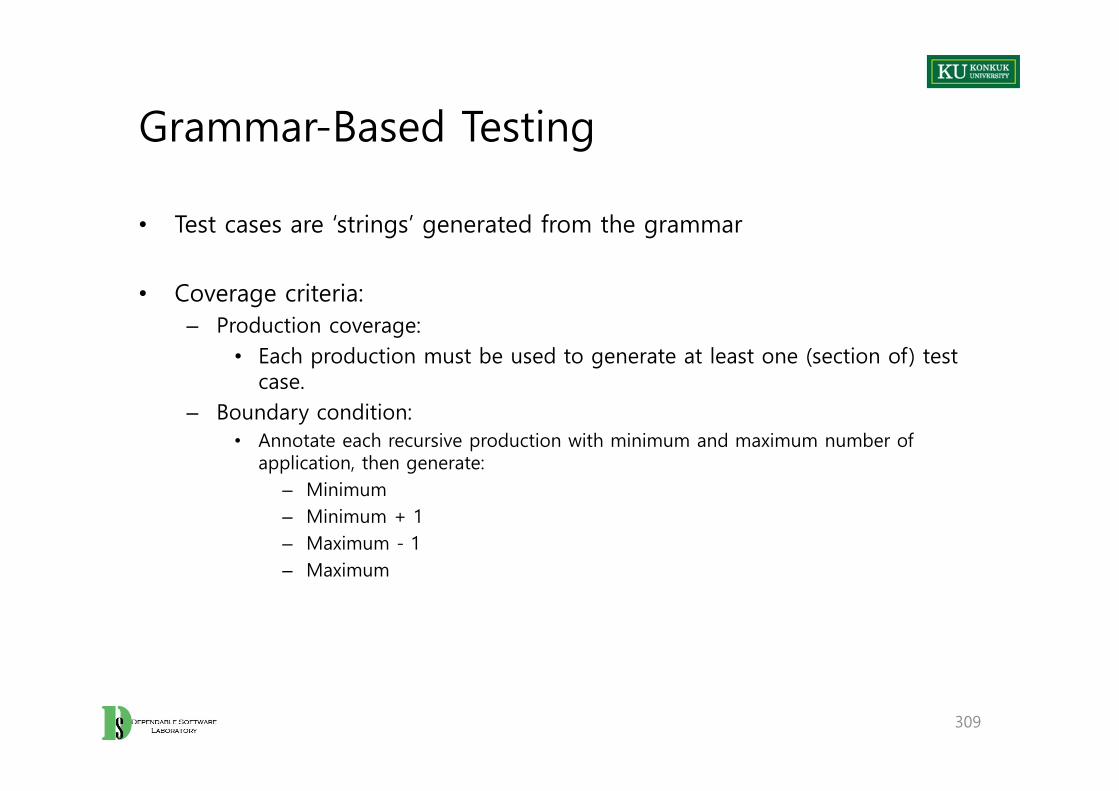
Grammar-Based Testing

• Test cases are ‘strings’ generated from the grammar

• Coverage criteria:– Production coverage:

• Each production must be used to generate at least one (section of) test case.

– Boundary condition: • Annotate each recursive production with minimum and maximum number of

application, then generate:– Minimum– Minimum + 1– Maximum - 1– Maximum

309

Informal Specification: Feature “Check Configuration” of the Chipmunk Web Site

Check configuration: The Check-configuration function checks the validity of a computer configuration.

Model: A model identifies a specific product and determines a set of constraints on available components. Models are characterized by logical slots for components, which may or may not be implemented by physical slots on a bus. Slots may be required or optional. Required slots must be assigned with a suitable component to obtain a legal configuration, while optional slots may be left empty or filled depending on the customers' needs

Example: The required ``slots'' of the Chipmunk C20 laptop computer include a screen, a processor, a hard disk, memory, and an operating system. (Of these, only the hard disk and memory are implemented using actual hardware slots on a bus.) The optional slots include external storage devices such as a CD/DVD writer.

Set of Components: A set of [slot,component] pairs, which must correspond to the required and optional slots associated with the model. A component is a choice that can be varied within a model, and which is not designed to be replaced by the end user. Available components and a default for each slot is determined by the model. The special value empty is allowed (and may be the default selection) for optional slots. In addition to being compatible or incompatible with a particular model and slot, individual components may be compatible or incompatible with each other.

Example: The default configuration of the Chipmunk C20 includes 20 gigabytes of hard disk; 30 and 40 gigabyte disks are also available. (Since the hard disk is a required slot, empty is not an allowed choice.) The default operating system is RodentOS 3.2, personal edition, but RodentOS 3.2 mobile server edition may also be selected. The mobile server edition requires at least 30 gigabytes of hard disk.

310

※ It is not the example in the text.

Corresponding Grammar with Limits

311

Model <Model>::= <modelNumber> <compSequence> <optCompSequence>

compSeq1 [0, 16] <compSequence> ::= <Component> <compSequence>

compSeq2 <compSequence> ::= empty

optCompSeq1 [0, 16] <optCompSequence> ::= <OptionalComponent> <optCompSequence>

optCompSeq2 <optCompSequence> ::= empty

Comp <Component> ::= <ComponentType> <ComponentValue>

OptComp <OptionalComponent> ::= <ComponentType>

modNum <modelNumber> ::= string

CompTyp <ComponentType> ::= string

CompVal <ComponentValue> ::= string

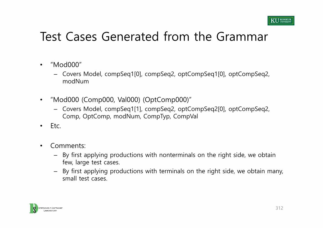
Test Cases Generated from the Grammar

• “Mod000”– Covers Model, compSeq1[0], compSeq2, optCompSeq1[0], optCompSeq2,

modNum

• “Mod000 (Comp000, Val000) (OptComp000)”– Covers Model, compSeq1[1], compSeq2, optCompSeq2[0], optCompSeq2,

Comp, OptComp, modNum, CompTyp, CompVal

• Etc.

• Comments:– By first applying productions with nonterminals on the right side, we obtain

few, large test cases.– By first applying productions with terminals on the right side, we obtain many,

small test cases.

312

Grammar Testing vs. Combinatorial Testing

• Combinatorial specification-based testing is good for “mostly independent” parameters.

– We can incorporate a few constraints, but complex constraints are hard to represent and use.

– We must often “factor and flatten.”– E.g. separate “set of slots” into characteristics “number of slots” and predicates

about what is in the slots (all together)

• Grammar describes sequences and nested structure naturally.– But, some relations among different parts may be difficult to describe and

exercise systematically, e.g. compatibility of components with slots.

313

Summary

• Models are useful abstractions.– In specification and design, they help us think and communicate about

complex artifacts by emphasizing key features and suppressing details.– Models convey structure and help us focus on one thing at a time.

• We can use them in systematic testing.– If a model divides behavior into classes, we probably want to exercise each of

those classes.– Common model-based testing techniques are based on state machines,

decision structures, and grammars.– But, we can apply the same approach to other models.

314

315

Chapter 15. Testing Object-Oriented Software

317

Chapter 16. Fault-Based Testing

Learning Objectives

• Understand the basic ideas of fault-based testing– How knowledge of a fault model can be used to create useful tests and judge

the quality of test cases– Understand the rationale of fault-based testing well enough to distinguish

between valid and invalid uses

• Understand mutation testing as one application of fault-based testing principles

319

Estimating Test Suite Quality

• Supposed that I have a program with bugs.

• Add 100 new bugs– Assume they are exactly like real bugs in every way– I make 100 copies of my program, each with one of my 100 new bugs.

• Run my test suite on the programs with seeded bugs– And the tests revealed 20 of the bugs. – The other 80 program copies do not fail.

• What can I infer about my test suite’s quality?

320

Basic Assumptions

• We want to judge effectiveness of a test suite in finding real faults, – by measuring how well it finds seeded fake faults.

• Valid to the extent that the seeded bugs are representative of real bugs– Not necessarily identical– But, the differences should not affect the selection

321

Mutation Testing

• A mutant is a copy of a program with a mutation.

• A mutation is a syntactic change (a seeded bug).– Example: change (i < 0) to (i <= 0)

• Run test suite on all the mutant programs• A mutant is killed, if it fails on at least one test case. (The bug is found.)

• If many mutants are killed, infer that the test suite is also effective at finding real bugs.

322

Assumptions on Mutation Testing

• Competent programmer hypothesis– Programs are nearly correct.

• Real faults are small variations from the correct program.• Therefore, mutants are reasonable models of real buggy programs.

• Coupling effect hypothesis– Tests that find simple faults also find more complex faults.– Even if mutants are not perfect representatives of real faults, a test suite that

kills mutants is good at finding real faults too.

323

Mutant Operators

• Syntactic changes from legal program to illegal program– Specific to each programming language

• Examples: – crp: constant for constant replacement

• E.g. from (x < 5) to (x < 12)• Select constants found somewhere in program text

– ror: relational operator replacement• E.g. from (x <= 5) to (x < 5)

– vie: variable initialization elimination• E.g. change int x =5; to int x;

324

Fault-based Adequacy Criteria

• Mutation analysis consists of the following steps:1. Select mutation operators2. Generate mutants3. Distinguish mutants

• Live mutants– Mutants not killed by a test suite

• Given a set of mutants SM and a test suite T, the fraction of nonequivalence mutants killed by T measures the adequacy of T with respect to SM.

325

Variations on Mutation Analysis

• Problem: – There are lots of mutants. – Running each test case to completion on every mutant is expensive.– Number of mutants grows with the square of program size.

• Solutions:– Weak mutation:

• Execute meta-mutant (with many seeded faults) together with original program

– Statistical mutation• Just create a random sample of mutants

326

Summary

• Fault-based testing is a widely used in semiconductor manufacturing.– With good fault models of typical manufacturing faults, e.g. “stuck-at-one” for

a transistor– But, fault-based testing for design errors is more challenging (as in software).

• Mutation testing is not widely used in industry.– But, plays a role in software testing research, to compare effectiveness of

testing techniques

327

328

Chapter 17. Test Execution

Learning Objectives

• Appreciate the purpose of test automation– Factoring repetitive and mechanical tasks from creative and human design

tasks in testing

• Recognize main kinds and components of test scaffolding

• Understand some key dimensions in test automation design– Design for testability: Controllability and observability– Degrees of generality in drivers and stubs– Comparison-based oracles and self-checks

330

Automating Test Execution

• Designing test cases and test suites is creative.– Demanding intellectual activity– Requiring human judgment

• Executing test cases should be automatic.– Design once, execute many times

• Test automation separates the creative human process from the mechanical process of test execution.

331

From Test Case Specifications to Test Cases

• Test design often yields test case specifications, rather than concrete data.– E.g. “a large positive number”, not 420,023– E.g. “a sorted sequence, length > 2”, not “Alpha, Beta, Chi, Omega”

• Other details for execution may be omitted.

• Test Generation creates concrete, executable test cases from test case specifications.

• A Tool chain for test case generation & execution– A combinatorial test case generation to create test data

• Optional: Constraint-based data generator to “concretize” individual values, e.g., from “positive integer” to 42

– ‘DDSteps’ to convert from spreadsheet data to ‘JUnit’ test cases– ‘JUnit’ to execute concrete test cases

332

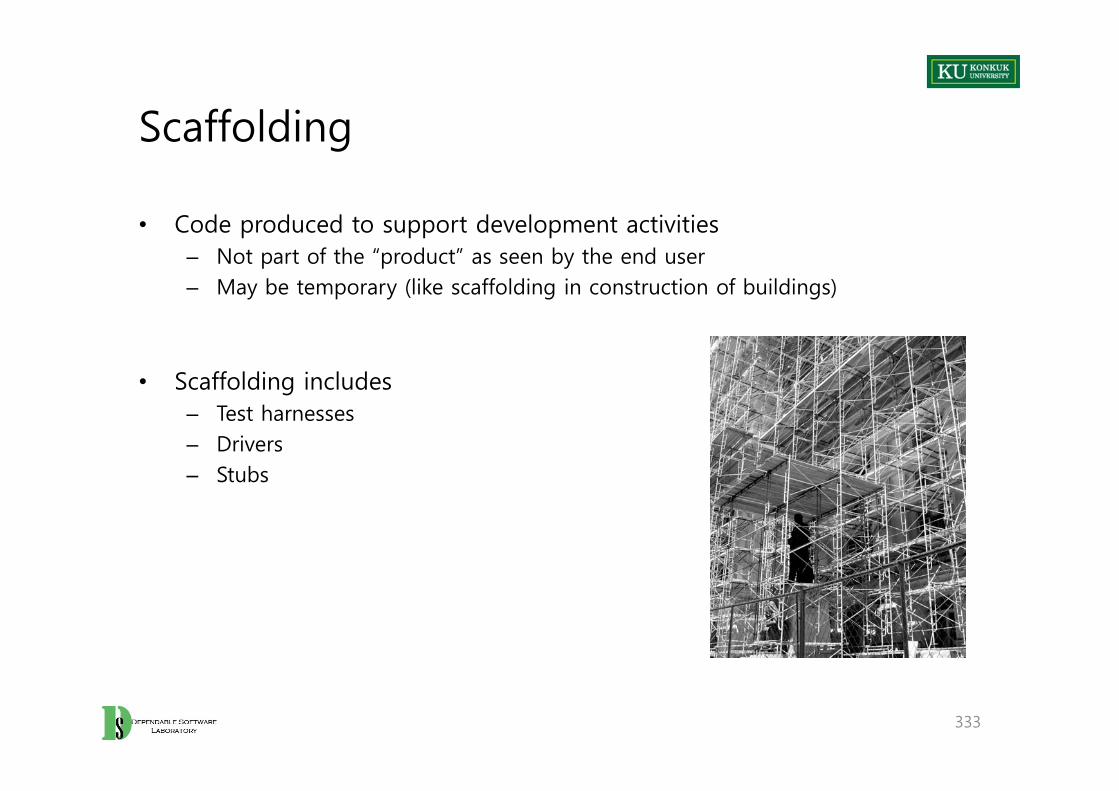
Scaffolding

• Code produced to support development activities– Not part of the “product” as seen by the end user– May be temporary (like scaffolding in construction of buildings)

• Scaffolding includes – Test harnesses– Drivers– Stubs

333

Scaffolding

• Test driver– A “main” program for running a test

• May be produced before a “real” main program• Provide more control than the “real” main program

– To drive program under test through test cases

• Test stub– Substitute for called functions/methods/objects

• Test harness– Substitutes for other parts of the deployed environment– E.g. Software simulation of a hardware device

334

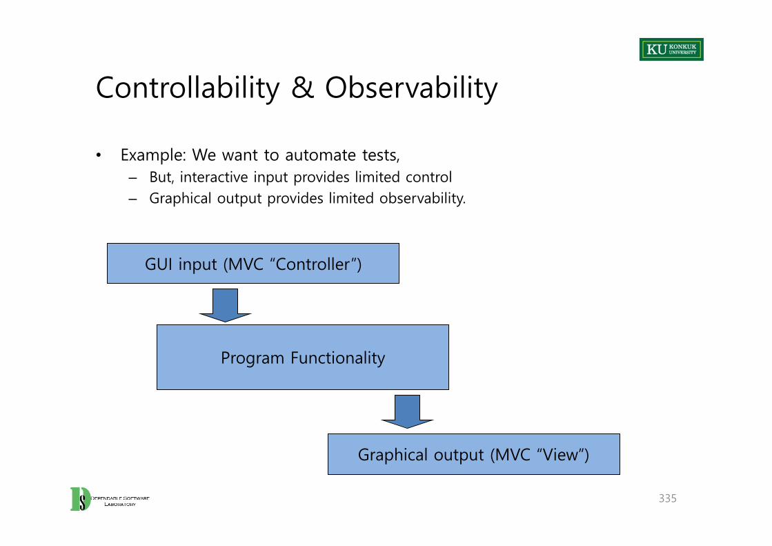
Controllability & Observability

• Example: We want to automate tests, – But, interactive input provides limited control– Graphical output provides limited observability.

335

GUI input (MVC “Controller”)

Program Functionality

Graphical output (MVC “View”)

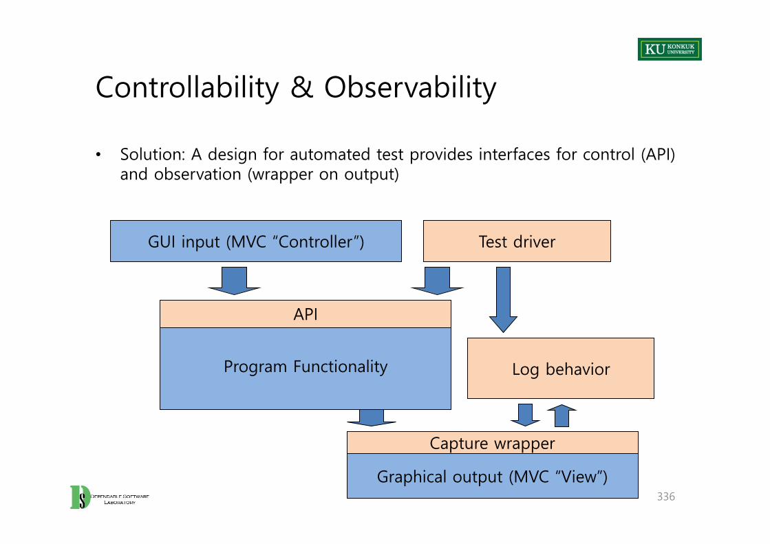
Controllability & Observability

• Solution: A design for automated test provides interfaces for control (API) and observation (wrapper on output)

336

GUI input (MVC “Controller”)

Program Functionality

Graphical output (MVC “View”)

API

Test driver

Capture wrapper

Log behavior

Generic vs. Specific Scaffolding

• How general should scaffolding be?– We could build a driver and stubs for each test case.– Or at least factor out some common code of the driver and test management

(e.g. JUnit)– Or further factor out some common support code, to drive a large number of

test cases from data (as in DDSteps)– Or further generate the data automatically from a more abstract model (e.g.

network traffic model)

• It’s a question of costs and re-use, just as for other kinds of software.

337

Test Oracles

• No use running 10,000 test cases automatically, if the results must be checked by hand.

• It’s a problem of ‘range of specific to general’, again– E.g. JUnit: Specific oracle (“assert”) coded by hand in each test case

• Typical approach– Comparison-based oracle with predicted output value– But, not the only approach

338

Comparison-based Oracle

• With a comparison-based oracle, we need predicted output for each input.

– Oracle compares actual to predicted output, and reports failure if they differ.– Fine for a small number of hand-generated test cases– E.g. for hand-written JUnit test cases

339

Self-Checks as Oracles

• An oracle can also be written as self-checks.– Often possible to judge correctness without predicting results

• Advantages and limits: Usable with large, automatically generated test suites, but often only a partial check

– E.g. structural invariants of data structures– Recognize many or most failures, but not all

340

Capture and Replay

• Sometimes there is no alternative to human input and observation.– Even if we separate testing program functionality from GUI, some testing of

the GUI is required.

• We can at least cut repetition of human testing.

• Capture a manually run test case, and replay it automatically– With a comparison-based test oracle: behavior be same as previously

accepted behavior– Reusable only until a program change invalidates it– Lifetime depends on abstraction level of input and output.

341

Summary

• Test automation aims to separate creative task of test design from mechanical task of test execution.

– Enable generation and execution of large test suites– Re-execute test suites frequently (e.g. nightly or after each program change)

• Scaffolding: Code to support development and testing– Test drivers, stubs, harness, oracles– Ranging from individual, hand-written test case drivers to automatic

generation and testing of large test suites– Capture/replay where human interaction is required

342

343

Chapter 18. Inspection

345

Chapter 19. Program Analysis

Learning Objectives

• Understand how automated program analysis complements testing and manual inspection

– Most useful for properties that are difficult to test

• Understand fundamental approaches of a few representative techniques– Lockset analysis– Pointer analysis– Symbolic testing– Dynamic model extraction

• Recognize the same basic approaches and design trade-offs in other program analysis techniques

347

Overview

• Automated program analysis techniques complement test and inspection in two ways:

– Can exhaustively check some important properties• Which conventional testing is particularly ill-suited

– Can extract and summarize information for test and inspection design• Replacing or augmenting human efforts

• Automated analysis– Replace human inspection for some class of faults– Support inspection by

• Automating extracting and summarizing information• Navigating through relevant information

348

Static vs. Dynamic Analysis

• Static analysis– Examine program source code

• Examine the complete execution space• But, may lead to false alarms

• Dynamic analysis– Examine program execution traces

• No infeasible path problem• But, cannot examine the execution space exhaustively

• Example:– Concurrency faults– Memory faults

349

Summarizing Execution Paths

• Our aim is to find all program faults of a certain kind.– We cannot simply prune exploration of certain program paths as in symbolic

testing.

• Instead, we must abstract enough to fold the state space down to a size that can be exhaustively explored.

– Example: analyses based on finite state machines (FSM)• data values by states• operations by state transitions

– The approaches taken in flow analysis and finite state verification

350

Memory Analysis

• Instrument program to trace memory access dynamically– Record the state of each memory location– Detect accesses incompatible with the current state

• Attempts to access unallocated memory • Read from uninitialized memory locations

– Array bounds violations:• Add memory locations with state unallocated before and after each array• Attempts to access these locations should be detected immediately

– Example:• Purify• Garbage detector

351

Pointer Analysis

• Pointer variables are represented by a machine with three states:– invalid value– possibly null value– definitely not null value

• Deallocation triggers transition from non-null to invalid.• Conditional branches may trigger transitions.

– E.g. testing a pointer for non-null triggers a transition from possibly null to definitely non-null

• Potential misuse – Deallocation in possibly null state – Dereference in possibly null – Dereference in invalid states

352

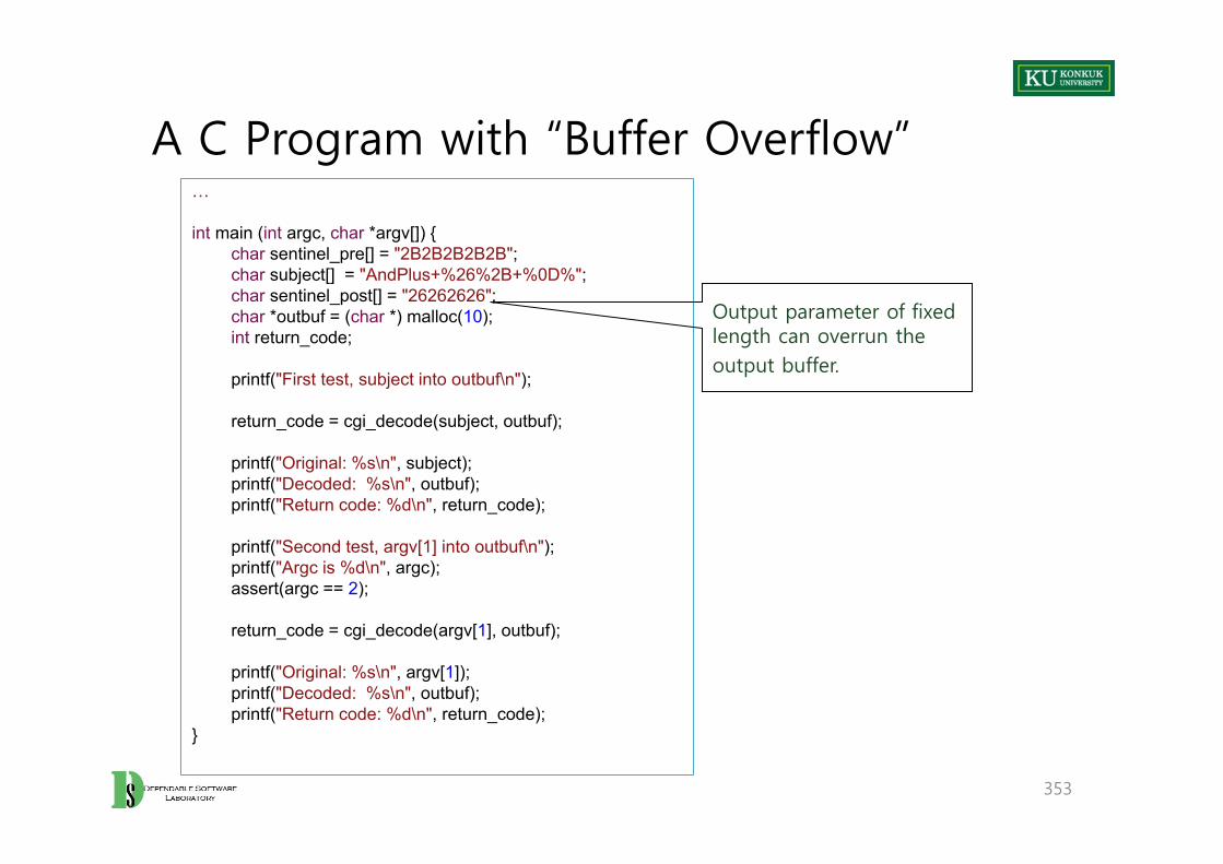
A C Program with “Buffer Overflow”

353

…

int main (int argc, char *argv[]) { char sentinel_pre[] = "2B2B2B2B2B"; char subject[] = "AndPlus+%26%2B+%0D%"; char sentinel_post[] = "26262626"; char *outbuf = (char *) malloc(10); int return_code;

printf("First test, subject into outbuf\n");

return_code = cgi_decode(subject, outbuf);

printf("Original: %s\n", subject);printf("Decoded: %s\n", outbuf);printf("Return code: %d\n", return_code);

printf("Second test, argv[1] into outbuf\n"); printf("Argc is %d\n", argc); assert(argc == 2);

return_code = cgi_decode(argv[1], outbuf);

printf("Original: %s\n", argv[1]); printf("Decoded: %s\n", outbuf); printf("Return code: %d\n", return_code);

}

Output parameter of fixed length can overrun theoutput buffer.

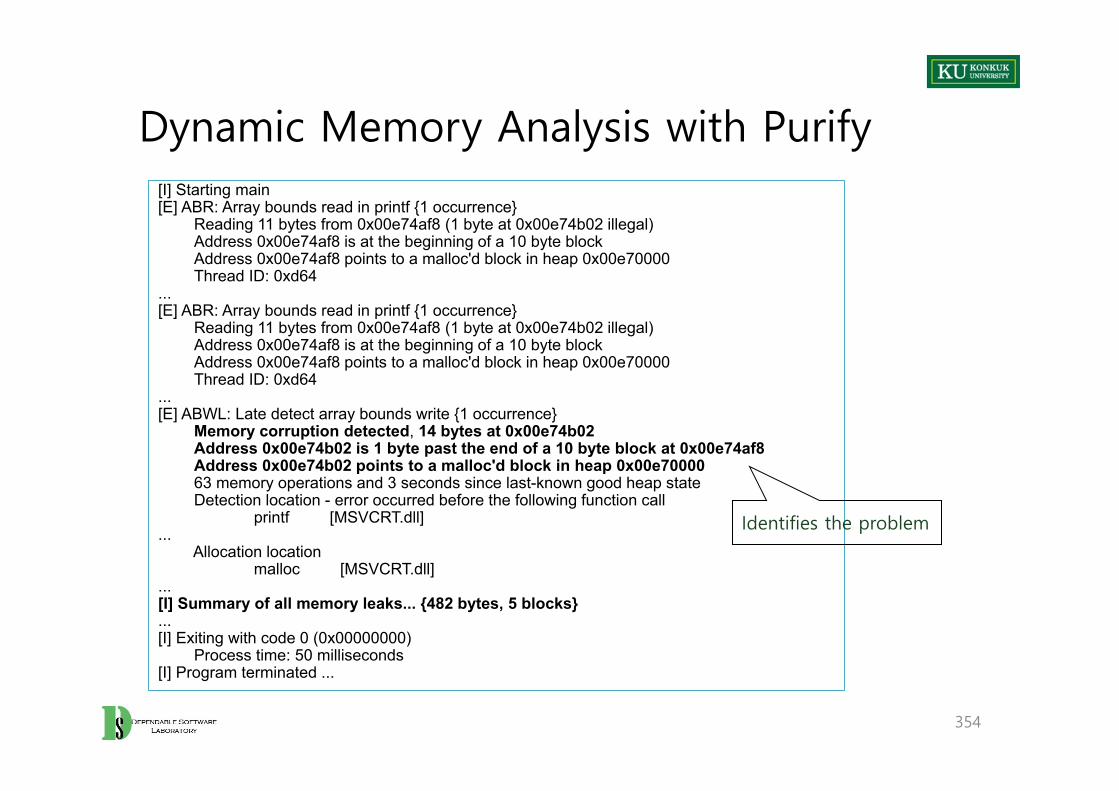
Dynamic Memory Analysis with Purify

354

[I] Starting main[E] ABR: Array bounds read in printf {1 occurrence}

Reading 11 bytes from 0x00e74af8 (1 byte at 0x00e74b02 illegal)Address 0x00e74af8 is at the beginning of a 10 byte blockAddress 0x00e74af8 points to a malloc'd block in heap 0x00e70000Thread ID: 0xd64

...[E] ABR: Array bounds read in printf {1 occurrence}

Reading 11 bytes from 0x00e74af8 (1 byte at 0x00e74b02 illegal)Address 0x00e74af8 is at the beginning of a 10 byte blockAddress 0x00e74af8 points to a malloc'd block in heap 0x00e70000Thread ID: 0xd64

...[E] ABWL: Late detect array bounds write {1 occurrence}

Memory corruption detected, 14 bytes at 0x00e74b02Address 0x00e74b02 is 1 byte past the end of a 10 byte block at 0x00e74af8Address 0x00e74b02 points to a malloc'd block in heap 0x00e7000063 memory operations and 3 seconds since last-known good heap stateDetection location - error occurred before the following function call

printf [MSVCRT.dll]...

Allocation locationmalloc [MSVCRT.dll]

...[I] Summary of all memory leaks... {482 bytes, 5 blocks}...[I] Exiting with code 0 (0x00000000)

Process time: 50 milliseconds[I] Program terminated ...

Identifies the problem

Lockset Analysis

• Data races are hard to reveal with testing.

• Static analysis:– Computationally expensive, and approximated

• Dynamic analysis:– Can amplify sensitivity of testing to detect potential data races

• Avoid pessimistic inaccuracy of finite state verification• Reduce optimistic inaccuracy of testing

355

Dynamic Lockset Analysis

• Lockset discipline: set of rules to prevent data races– Every variable shared between threads must be protected by a mutual

exclusion lock.– ….

• Dynamic lockset analysis detects violation of the locking discipline.– Identify set of mutual exclusion locks held by threads when accessing each

shared variable.– INIT: each shared variable is associated with all available locks– RUN: thread accesses a shared variable

• intersect current set of candidate locks with locks held by the thread

– END: set of locks after executing a test = set of locks always held by threads accessing that variable

• empty set for v = no lock consistently protects v

356

Simple Lockset Analysis: An Example

357

Thread Program trace Locks held Lockset(x)

{} {lck1, lck2}

thread A lock(lck1)

{lck1}

x=x+1

{lck1}

unlock(lck1}

{}

tread B lock{lck2}

{lck2}

x=x+1

{}

unlock(lck2}

{}

INIT:all locks for x

lck1 held

Intersect with locks held

lck2 held

Empty intersection potential race

Lockset Analysis in Practice

• Simple locking discipline violated by – Initialization of shared variables without holding a lock– Writing shared variables during initialization without locks– Allowing multiple readers in mutual exclusion with single writers

358

Delay analysistill after initialization

(second thread) Multiple writers

report violations

Multiple readers single writerdo not report violations

Extracting Behavior Model from Execution

• Behavior analysis can– Gather information from executing several test cases– And synthesize a model that characterizes those execution,– To the extent that they are the representative of other executions as well.

• Using behavioral models for– Testing : validate tests thoroughness

– Program analysis : understand program behavior

– Regression testing : compare versions or configurations

– Testing of component-based software : compare components in different contexts

– Debugging : Identify anomalous behaviors and understand causes

359

Summary

• Program analysis complements testing and inspection.– Addresses problems (e.g., race conditions, memory leaks) for which

conventional testing is ineffective– Can be tuned to balance exhaustiveness, precision and cost (e.g., path-

sensitive or insensitive)– Can check for faults or produce information for other uses (debugging,

documentation, testing)

• A few basic strategies– Build an abstract representation of program states by monitoring real or

simulated (abstract) execution

360

361

Part IV. Process

Chapter 20. Planning and Monitoring the Process

Chapter 21. Integration and Component-based

Software Testing

Chapter 22. System, Acceptance, and Regression

Testing

Chapter 23. Automating Analysis and Test

Chapter 24. Documenting Analysis and Test