So

ftwa

re P

erf

orm

an

ce

Op

timis

atio

n G

rou

p

Generating GPU-Accelerated Code From a High-level Domain-specific Language

Graham MarkallSoftware Performance Optimisation GroupImperial College Londonhttp://www.doc.ic.ac.uk/~grm08

Joint work with David Ham and Paul Kelly

October 2009

So

ftwa

re P

erf

orm

an

ce

Op

timis

atio

n G

rou

pProblem & Proposal

How do we exploit multicore architectures to improve the performance of the Assembly Phase?

Writing code for new architectures is time-consuming and error-prone

Provide hardware-independent abstraction for the specification of finite element methods.

Future proofing of codeEasier development

Background: Conjugate Gradient GPU Solver 10x faster than one CPU coreSolvers are generic – someone else will solve this problem

So

ftwa

re P

erf

orm

an

ce

Op

timis

atio

n G

rou

pThis Study

We present a pilot study into using the Unified Form Language to generate CUDA code.

Why bother with part 1? To prove we can speed up assembly using GPUsTo provide a guide for the output we expect from the compilerTo experiment with different performance optimisations

Part 1:1.Nvidia Tesla Architecture & CUDA2.Test Problems3.Translation Methodology4.Performance Optimisations5.Performance Results

Part 2:1.UFL2.UFL Compiler Design3.Test Results4.Discussion

So

ftwa

re P

erf

orm

an

ce

Op

timis

atio

n G

rou

pNVIDIA Tesla Architecture & CUDA

GT200 Architecture: 1-4GiB RAM

For high performance:Coalescing:

Use many threads (10000+)

Caches:Texture cache (read-only)Shared memory

64B window

16 threads (half-warp)

Data transfer

Data transfer

So

ftwa

re P

erf

orm

an

ce

Op

timis

atio

n G

rou

pThe Test Problems

Test_laplacian: Solves ∆u = f on unit squareAnalytical solution: Allows us to examine the accuracy of the computed solution

Test_advection_diffusion:

Advection-Diffusion is more representative:Time-dependent, nonlinear multiple assemble/solve

So

ftwa

re P

erf

orm

an

ce

Op

timis

atio

n G

rou

pFrom Fortran to CUDA (Test_laplacian)

Assembly Loop in Fortran:

Assembly Loop in CUDA:

1 Element

All Elements

do ele=1,num_ele call assemble(ele,A,b)end do

call petsc_solve(x,A,b)

call gpu_assemble()

call gpucg_solve(x)

So

ftwa

re P

erf

orm

an

ce

Op

timis

atio

n G

rou

pFrom Fortran to CUDA (Adv.-Diff.)

Original:AssembleSolveOutput of solve input to next Assemble

CUDA:Avoid transferring the solution at every iterationUpload initial conditionsIterateTransfer solution when required

So

ftwa

re P

erf

orm

an

ce

Op

timis

atio

n G

rou

p

CoalescingMaximise memorybandwidth

Performance Optimisations

...(x1,y1)

(x2,y2) (x3,y3)

...

123

n-2n-1

n

x1 y1 x2 y2 x3 y3 1 2 3

x1 y1

x2

y2

x3

y3

n-2 n-1 n

So

ftwa

re P

erf

orm

an

ce

Op

timis

atio

n G

rou

p

CoalescingMaximise memorybandwidth

Specialisation of Kernels (reduced register usage)

Performance Optimisations

for(int x=0; x<nodes; x++) { for(int y=0; y<nodes; y++) { ...; }}

for(int x=0; x<3; x++) { for(int y=0; y<3; y++) { ...; }}

...(x1,y1)

(x2,y2) (x3,y3)

...

123

n-2n-1

n

x1 y1 x2 y2 x3 y3 1 2 3

x1 y1

x2

y2

x3

y3

n-2 n-1 n

So

ftwa

re P

erf

orm

an

ce

Op

timis

atio

n G

rou

p

CoalescingMaximise memorybandwidth

Specialisation of Kernels (reduced register usage)

Texture Memory for matrix sparsity

Performance Optimisations

for(int x=0; x<nodes; x++) { for(int y=0; y<nodes; y++) { ...; }}

for(int x=0; x<3; x++) { for(int y=0; y<3; y++) { ...; }}

...(x1,y1)

(x2,y2) (x3,y3)

...

123

n-2n-1

n

x1 y1 x2 y2 x3 y3 1 2 3

x1 y1

x2

y2

x3

y3

n-2 n-1 n

col_idx

val

row_ptr

So

ftwa

re P

erf

orm

an

ce

Op

timis

atio

n G

rou

pPerformance Results

For Advection-Diffusion problem. Test setup:Nvidia 280GTX – 1GB RAM (use Tesla C1060 for 4GB)Intel Core 2 Duo E8400 @ 3.00GHz2GB RAM in host machineIntel C++ and Fortran Compilers V10.1

V11.0 suffers from bugs and cannot compile FluidityCPU Implementations compiled with –O3 flagsCUDA Implementation compiled using NVCC 2.2

Run problem for 200 timestepsIncreasingly fine meshes

Increasing element countFive runs of each problem

Averages reportedDouble Precision computations

So

ftwa

re P

erf

orm

an

ce

Op

timis

atio

n G

rou

pAdvection Diffusion Assembly Time

So

ftwa

re P

erf

orm

an

ce

Op

timis

atio

n G

rou

pSpeedup in the Assembly Phase

So

ftwa

re P

erf

orm

an

ce

Op

timis

atio

n G

rou

pOverall Speedup (Assemble & Solve)

So

ftwa

re P

erf

orm

an

ce

Op

timis

atio

n G

rou

pProportion of GPU Time in each Kernel

Which kernels should we focus on optimising?

Addto kernels: 84% of execution time

So

ftwa

re P

erf

orm

an

ce

Op

timis

atio

n G

rou

pThe Impact of Atomic Operations

Colouring Optimisation on GPUs: [1] D. Komatitsch, D.Michea and G. Erlebacher. Porting a high-order finite-element earthquake modelling application to Nvidia graphics cards using CUDA. J. Par. Dist. Comp., 69(5):451-460, 2009

So

ftwa

re P

erf

orm

an

ce

Op

timis

atio

n G

rou

pSummary of Part 1

8x Speedup over 2 CPU Cores for assembly6x Speedup overallFurther performance gains from:

Colouring Elements & Non-atomic ops [1]Alternative matrix storage formatsFusing kernels [2], Mesh partitioning [3]

Fusing kernels: [2] J. Filipovic, I. Peterlik and J. Fousek. GPU Acceleration of Equations Assembly in Finite Elements Method – Preliminary Results. In SAAHPC: Symposium on Application Accelerators in HPC, July 2009.Mesh partitioning: [3] A. Klockner, T. Warburton, J. Bridge and J. S. Hesthaven. Nodal Discontinuous Galerkin methods on graphics processors. Journal of Computational Physics, in press, 2009.

So

ftwa

re P

erf

orm

an

ce

Op

timis

atio

n G

rou

p

Solving:Weak form:

(Ignoring boundaries)

Close to mathematical notationNo implementation details

Allows code generation for multiple backends and choice of optimisations to be explored.

Part 2: A UFL [4] Example (Laplacian)

Psi = state.scalar_fields(“psi”)v=TestFunction(Psi)u=TrialFunction(Psi)f=Function(Psi, “sin(x[0])+cos(x[1])”)A=dot(grad(v),grad(u))*dxRHS=v*f*dxSolve(Psi,A,RHS)

[4] M. Alnaes and Anders Logg. Unified Form Language Specification and User’s Manual. http://www.fenics.org/pub/documents/ufl/ufl-user-manual/ufl-user-manual.pdf Retrieved 15 Sep 2009.

So

ftwa

re P

erf

orm

an

ce

Op

timis

atio

n G

rou

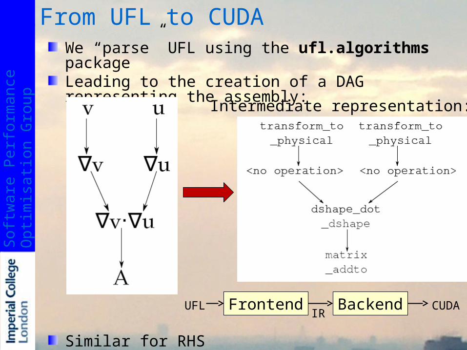
pFrom UFL to CUDA

We “parse” UFL using the ufl.algorithms packageLeading to the creation of a DAG representing the assembly:

Similar for RHS

Intermediate representation:

Frontend BackendUFLIR

CUDA

So

ftwa

re P

erf

orm

an

ce

Op

timis

atio

n G

rou

p

Hand Translation: Generated Code:

TestingBackend (example):stringList *params = new stringList();(*params).push_back(string("val"));(*params).push_back(string("size_val"));(*params).push_back(string("ele_psi"));(*params).push_back(string("lmat"));(*params).push_back(string("n"));launchList.push_back( kernelLaunch("matrix_addto",params));

Frontend:psi = state.scalar_fields("psi")v = TestFunction(P)u = TrialFunction(P)f = Function(P)f.name="shape_rhs"A = dot(grad(v),grad(u))*dxsolve(P, A, f)

So

ftwa

re P

erf

orm

an

ce

Op

timis

atio

n G

rou

pTesting - continued

Helmholtz equation:Weak form:

A=(dot(grad(v), grad(u))+(20)*dot(v,u))*dxAdd extra calls to shape_shape and matrix_addto

FEniCS Dolfin solution: Generated code solution:

So

ftwa

re P

erf

orm

an

ce

Op

timis

atio

n G

rou

pConclusions

We obtain speedups of 8x over 2 core CPU in the assembly phase using CUDA

An overall speedup of 6x over 2 cores

Generation of CUDA code from UFL source is feasible

UFL is “future proof”UFL is easier to use than CUDA, Fortran etc.Allows automated exploration of optimisationsOther backends (Cell, multicore CPU, Larrabee etc.) should be possible

So

ftwa

re P

erf

orm

an

ce

Op

timis

atio

n G

rou

pFurther workOn the UFL Compiler:

Support for a more complete subset of UFLDevelopment of a more expressive intermediate representation

Facilitates the development of other backends Generation of kernels from IR

Automatic tuning

On the Conjugate Gradient Solver:Integration with blocked SpMV implementation [5]

Expect: further performance improvements

Blocked SpMV: [5] A. Monakov and A. Avetisyan. Implementing Blocked Sparse Matrix-Vector Multiplication on Nvidia GPUs. In SAMOS IX: International Symposium on Systems, Architectures, Modeling and Simulation, July 2009.

So

ftwa

re P

erf

orm

an

ce

Op

timis

atio

n G

rou

pSpare Slides

So

ftwa

re P

erf

orm

an

ce

Op

timis

atio

n G

rou

pTest Advection Diffusion UFL

Advection:T=state.scalar_fields(Tracer)U=state.vector_fields(Velocity)UNew=state.vector_fields(NewVelocity)

# We are solving for the Tracer, T.t=Function(T)p=TrialFunction(T)q=TestFunction(T)

#The value of the advecting velocity U is known.u=Function(U)unew=Function(UNew)

#Mass matrix.M=p*q*dx

#Solve for T1-T4.rhs=dt*dot(grad(q),u)*t*dxt1=solve(M,rhs)rhs=dt*dot(grad(q),(0.5*u+0.5*unew))*(t+0.5*t1)*dxt2=solve(M,rhs)rhs=dt*dot(grad(q),(0.5*u+0.5*unew))*(t+0.5*t2)*dxt3=solve(M,rhs)

#Solve for T at the next time step.rhs=action(M,t) + 1.0/6.0*t1 + 1.0/3.0*t2 + 1.0/3.0*t3 + 1.0/6.0*t4t=solve(M,t)

Diffusion:mu=state.tensor_fields(TracerDiffusivity)i,j=indices(2)M=p*q*dxd=-grad(q)[i]*mu[i,j]*grad(p)[j]*dxA=m-0.5*drhs=action(M+0.5*d,t)T=solve(A,rhs)

So

ftwa

re P

erf

orm

an

ce

Op

timis

atio

n G

rou

pMemory Bandwidth Utilisation

Orange: Using Atomic operationsBlue: Using non-atomic operations

So

ftwa

re P

erf

orm

an

ce

Op

timis

atio

n G

rou

pProportion of GPU Time in each Kernel

Orange: Using Atomic operationsBlue: Using non-atomic operations

So

ftwa

re P

erf

orm

an

ce

Op

timis

atio

n G

rou

pAssembly Throughput

So

ftwa

re P

erf

orm

an

ce

Op

timis

atio

n G

rou

pCode Generation

List of variables, kernels and parameters passed to backend.Using the ROSE Compiler Infrastructure [6].

CUDA Keywords (__global__, <<<...>>> notation) inserted as arbitrary strings.

AST

gpu_assemble.cu

InitialisationcudaMalloc()cudaBindTexture()cudaMemcpy()

StreamingcudaMemcpy()

Assemblykernel<<<.>>>()

FinalisationcudaFree()cudaUnbindTexture()

DeclarationsInt, double, ...

So

ftwa

re P

erf

orm

an

ce

Op

timis

atio

n G

rou

pNVIDIA Tesla Architecture & CUDA

GT200 Architecture10 TPCs8 Banks of DRAM: 1-4GiB

y = αx + y in C:

CUDA Kernel:

__global__ void daxpy(double a, double* x, double* y, int n) { for (int i=T_ID; i<n; i+=T_COUNT) y[i] = y[i] + a*x[i];}

void daxpy(double a, double* x, double* y, int n) { for (int i=0; i<n; i++) y[i] = y[i] + a*x[i];}

So

ftwa

re P

erf

orm

an

ce

Op

timis

atio

n G

rou

pVariable naming

How do we ensure the output of a kernel is correctly input to successive kernels? Consistently invent names.

Psi = state.scalar_fields(“psi”)v=TestFunction(Psi)u=TrialFunction(Psi)f=Function(Psi, “sin(x[0])+cos(x[1])”)A=dot(grad(v),grad(u))*dxRHS=v*f*dxSolve(Psi,A,RHS)

Output: dshape_psi

Input: dshape_psiOutput: lmat_psi_psi

Input: lmat_psi_psi

So

ftwa

re P

erf

orm

an

ce

Op

timis

atio

n G

rou

pMemory Bandwidth Utilisation