SOFTWARE / HARDWARE PARTITIONING TECHNIQUES

SHaPES: A New Approach

Background

The allocation of a system’s functionality into hardware and software components has a significant impact on total system cost.

Partitioning algorithms usually target one of the following types of systems: Single-processor, single-ASIC (or FPGA) SOC Multiple processing element (PE),

distributed heterogeneous system

Background

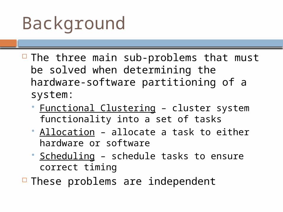
The three main sub-problems that must be solved when determining the hardware-software partitioning of a system: Functional Clustering – cluster system

functionality into a set of tasks Allocation – allocate a task to either hardware

or software Scheduling – schedule tasks to ensure correct

timing These problems are independent

Background

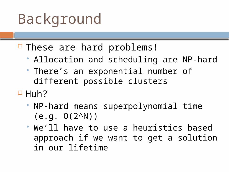
These are hard problems! Allocation and scheduling are NP-hard There’s an exponential number of different

possible clusters Huh?

NP-hard means superpolynomial time (e.g. O(2^N))

We’ll have to use a heuristics based approach if we want to get a solution in our lifetime

Background

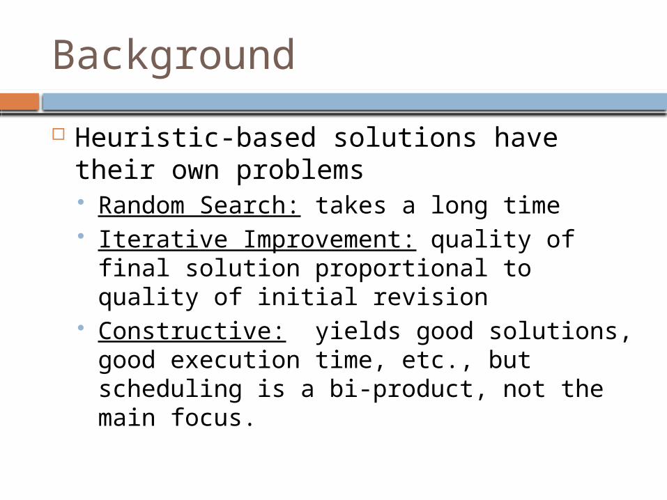
Heuristic-based solutions have their own problems Random Search: takes a long time Iterative Improvement: quality of final

solution proportional to quality of initial revision

Constructive: yields good solutions, good execution time, etc., but scheduling is a bi-product, not the main focus.

Who you gonna call?

SHaPES

“Software-Hardware Partitioning For Embedded Systems”

Formulating The Problem

This approach assumes a single microprocessor and single ASIC SOC as the target platform

Looks at the partitioning problem as a real-time scheduling problem… we’re scheduling a set of periodic and sporadic tasks

Tasks are implemented either completely in hardware or software

Formulating The Problem

Implementation Costs We Care About: Hardware Area Power Consumption Timing Constraints

But, a scheduling problem can’t model size and power constraints!

Formulating The Problem

Hard-timing constraints modeled as follows: Processing Time (pj): How long it takes a

task to execute on the microprocessor uninterupted

Release Time (rj): The earliest moment as which a task can begin execution

Deadline (dj): The time by which the task should be completed

Weight (wj): The importance of a task

Formulating The Problem

Under this model, all tasks start out initially in software. Rejecting a task implies it should be implemented in hardware.

Since hardware is always assumed to be fast-enough for a task, you could cheat and reject all tasks, but that’s not realistic

Formulating The Problem

Violations are modeled as “costs;” the further past the deadline a task completes and the higher the weight of the task, the higher the penalty

Delegating a task to hardware is also modeled as a cost, called the “rejection cost,” represented by ej

Formulating The Problem

Thus, the crux of the problem is:

Partition the set of tasks such that the sum of costs incurred by overtime software tasks and the rejection costs incurred by implementing a task in hardware are minimized

Formulating The Problem

But, sometimes a task has to wait around for other tasks to complete before they can start!

These dependencies are accounted for and are referred to as “precedence constraints” in the paper.

Solving The Scheduling Problem

Scheduling a set of jobs to minimize overall tardiness is an old problem (older than you)

Some simple approaches are: Earliest Due Date (EDD) Shortest Processing Time First (SPT)

This paper, however, uses ATC or Apparent Tardiness Cost

Solving The Scheduling Problem

Tasks are scheduled in non-increasing priority with priority defined as:

j

ii

i

i

p

ptd

p

w )}(,0max{1

Solving The Scheduling Problem

Note that the formula includes the processing time of the subsequent task

Thus, that value is replaced with kp, where p is the average execution time, and k is a look-ahead factor whose value depends on how many tasks are completing late.

Solving The Scheduling Problem

ATC dispatching is basically a proportion of the weight to the execution time, scaled by how much time you still have to schedule the task

Thus, the priority of a task increases the closer you are to its deadline

Good News: The algorithm still works pretty well even if your processing time estimates contain errors (but that’s another paper)

Dealing With Idleness

Basic Idea: ATC designates a task that should be run next, but its release time has not yet been reached. The system will have to sit idle until that time is reached.

Solution: Scale the priority of a task proportional to this idleness:

min

)}(,0max{1

p

tri

Rubber Hits The Road

Start with all tasks initially in software partition

At a given time t, take the task with the largest ATC

Multiply its weight by its tardiness (completion time – deadline)

If the above cost is greater than its rejection cost, reject it to hardware and pick another task

Rubber Hits The Road

Repeat this until you have an ordered set of software tasks, and a set of tasks that have been rejected to hardware.

Re-run the algorithm for the hardware tasks with appropriate processing times.

If you have no rejected hardware tasks, you’re done!

If you do have rejected hardware tasks, you need to pick different hardware and start over.

Questions