Software Engineering Prof.N.L.Sarda Lecture-11 Data...

Software Engineering

Prof.N.L.Sarda

IIT Bombay

Lecture-11

Data Modelling- ER diagrams,

Mapping to relational model

(Part -II)

We will continue our discussion on process modeling. In the previous lecture we talked

about functional decomposition as a first step in process modeling.

(Refer Slide Time 00:56)

Given a complex process we should try to decompose it into sub processes or smaller

processes which can be better understood in terms of what actions they do. We will now

continue with the process modeling and look at another important tool called data flow

diagrams. Data flow diagrams are a very popular tool for describing functions which are

required in a given system and these functions are specified in terms of processes as well

as the data used by these processes.


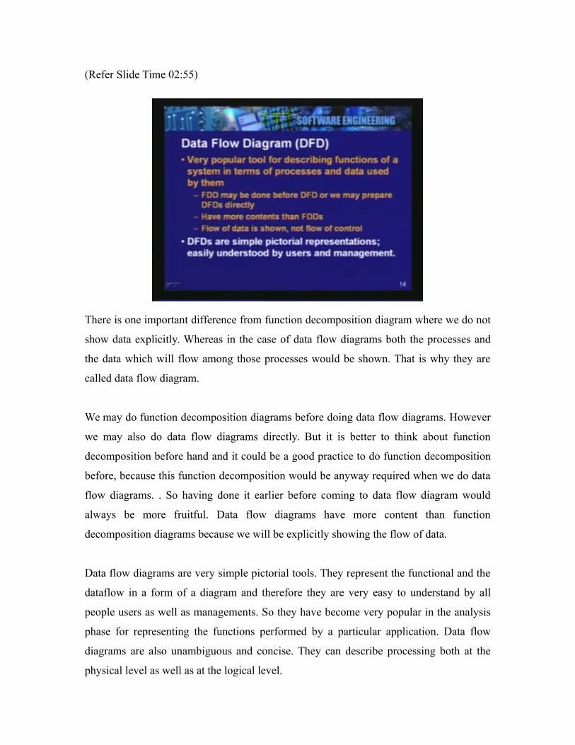
There is one important difference from function decomposition diagram where we do not

show data explicitly. Whereas in the case of data flow diagrams both the processes and

the data which will flow among those processes would be shown. That is why they are

called data flow diagram.

We may do function decomposition diagrams before doing data flow diagrams. However

we may also do data flow diagrams directly. But it is better to think about function

decomposition before hand and it could be a good practice to do function decomposition

before, because this function decomposition would be anyway required when we do data

flow diagrams. . So having done it earlier before coming to data flow diagram would

always be more fruitful. Data flow diagrams have more content than function

decomposition diagrams because we will be explicitly showing the flow of data.

Data flow diagrams are very simple pictorial tools. They represent the functional and the

dataflow in a form of a diagram and therefore they are very easy to understand by all

people users as well as managements. So they have become very popular in the analysis

phase for representing the functions performed by a particular application. Data flow

diagrams are also unambiguous and concise. They can describe processing both at the

physical level as well as at the logical level.


Remember that at the physical level we describe the way things are done rather than what

needs to be done. So we can have both data flow diagrams. In fact usually when you are

studying the existing system you are studying it at the physical level. Therefore if you

represent this in the form of a data flow diagram, the diagram will be at the physical level

representing both what is done and how it is done currently.

After doing this, you will move towards preparation of a logical level data flow diagram,

where we emphasize what needs to be done and not necessarily how it should be done

because the ‘how’ part is really the part to be addressed during the design phase. DFDs

facilitate top-down development. In fact that is the strength of the tool, so that you can

introduce more and more details as you do step by step decomposition of these diagrams.

They permit outlining of preferences and scope.

When you are discussing different alternatives with the users or the management you can

clearly mark those alternatives on the data flow diagram itself. So that people can

understand the scope of the application software that we are proposing. So is a another

use of data flow diagram. Here is the notation that we use in diagramming the data flows.

In the diagram you show the data flow through an arrow. Usually the arrow will be

labeled with the kind of the data which flows on that.


We show the sources of the data or the sources which use the information. These are

generally the external entities and these entities are shown using either a rectangle like

this or it may be a double edged rectangle. I am giving here two different representations

and both are used in the industry. You can choose one of them. The one on the left is

simpler to draw when we are doing the data flow diagrams by hand. But when you use

tools for doing data flow diagrams, any one of them could be used.

So, sources and sinks of data and information typically are users of the system and these

would be shown as external entities. Then the processes are either shown as a circle,

which is also called a bubble or a rectangle with rounded corners and we label them with

some number for easy reference. So process is shown. Then finally we also show data

either through a pair of lines or by a small box which represents a collection of data and

that box may also be labeled with a number for ease of referencing.

Primarily the data flow diagram provides only four symbols:

One is the arrow for flow of data.

One is a rectangle that represents an external entity which would either supply

some data to our application or which will receive some results from our

application.

Then we have the processes represented as bubbles.

And we have the data store which is represented by a pair of lines.

These are the simple notation that we will use for drawing data flow diagrams. Here is a

simple example. Let us begin by an example and you will also appreciate how simple

they are to read and understand.


Now in this, we see two rectangles both are labeled same, so it is a single entity called a

traveller. Traveller is an external entity which will be using this application which we

have called as ‘Air line reservation’. Some data flows from this traveller and comes to a

process called ‘make reservation’. That data would be the date and time and destination

where the traveller wishes to go and he wants to buy a ticket if it is available.

The first process which handles this data is the ‘make reservation’ process. If you look at

this process, this process not only takes the input from traveller, but it takes another input

from a data source called flight database. This arrow the direction of arrow indicates that

the data is being taken by the process; it is an input of data. So we take two inputs here,

one is from the traveler about his time date and destination, the other is the flight

database.

And then we prepare a suitable reservation, the reservation is also recorded. We may have

to consult the existing bookings and see whether there is a space available. If available

we make a reservation.

After making the reservation, this process produces outputs for two other processes. One

output goes from make reservation to a process called ‘prepare ticket’. Ideally we should

be labeling all these arrows. The label of the arrow will indicate the data which is sent by

make reservation to the prepare ticket.

But from the context we can easily make out that in order to prepare the ticket we will

have to obtain the travelers data as well as the flight data. So that the ticket can be made.

The ticket is an output of this process. The ticket goes to the traveler. So this is the

physical output produced by our software for the traveler.

There is another process to which the ‘make reservation’ process supplies some output

and that process is the billing system. Again we can easily see that the billing system

must receive some inputs from ‘make reservation’. So that the cost of the journey or the

cost of the ticket can be calculated and this billing system will produce a bill for the

traveler. And will also note that in the accounting file, subsequently it will also handle the

payment from the traveler.

So, in this airline reservation we have defined three processes called make reservation,

prepare ticket and billing system. We have identified one external entity who is the user

of this software or this application and we have identified the data stores. These data

stores contain the data relevant to the application; these data may be related to the flights,

these data may be related to the customer himself for the system to keep the billing

information for him and also the data about the bookings that we have been we have

made. So Air line reservation system would consist of such processes.

So you see here, the data flow diagram can be read in terms of external entities, the data

that they supply or the result that they receive and we can through the names that we have

selected for these processes, we can try to understand what happens in this application.

So its again the naming is very important. We named the bubbles as well as the data

sources properly. And when we do that a data flow diagram can be understood easily

without any additional explanation from the analyst. This is the advantage of the data

flow diagrams; they are understandable on their own. When we start the designing or

developing the data flow diagram, we can generally show the entire application as a

single process itself.


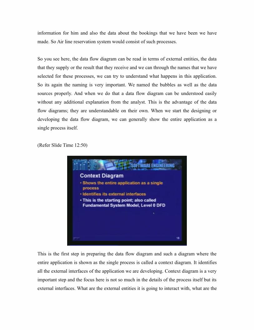
This is the first step in preparing the data flow diagram and such a diagram where the

entire application is shown as the single process is called a context diagram. It identifies

all the external interfaces of the application we are developing. Context diagram is a very

important step and the focus here is not so much in the details of the process itself but its

external interfaces. What are the external entities it is going to interact with, what are the

outputs it will produce, what are the existing data stores that it might have to interface in

terms of obtaining the data or updating that data.

This is usually the starting point and it is also called fundamental system model or the

level zero data flow diagram. So you do the data flow diagram in steps by successively

refining the different processes or by successively decomposing those processes and in

this you add more and more details. But the starting point is always the context diagram

in which the focus is on the external interfaces of the software. Here is the simple

example of a context diagram, in which the whole software application that we are

developing is shown as a single process or a single bubble.


We identify the users, the inputs and the outputs that system either receives or produces.

We also identify existing sources of data. These existing sources contain the data which is

useful for our application, but they exist outside. By showing it in the context diagram we

are clearly saying that this data store will be assumed to be an existing data store and it

will not be part of our development and design effort. That is the boundary. We are

defining clearly the boundary of the software that we want to develop. We also identify

other external sources which may be necessary for interfacing our application with other

applications. These may be messages or they may be data stores which will be interfacing

with external system. So context diagram is a very important first step in preparing the

data flow diagram.

After we have done the context diagram, we now decompose the process in to its sub

process. Here is the process decomposition now coming in the picture.


When we do this, we replace the process by its constituent sub processes. In this, we may

reveal additional data stores or additional external interfaces. So we are adding now more

and more details and we also develop some simple kind of a simple numbering system

through which we can readily show the constituent processes of a process which we have

decomposed.

Generally we use the decimal numbering system. If we are decomposing process1, then

the sub processes of that would be numbered as 1.1, 1.2 etc. This is for ease of

understanding the decomposition relationship between the processes. At each level of

decomposition, we should complete the data flow diagram in its all respects. We must

clearly understand the data which is flowing. We must know what exactly goes from one

process to another process or what goes from one data store to a process.

These must be properly labeled, we must also label the processes very meaningfully. In

fact, we had earlier mentioned that processes are best named by a verb and a object. We

had seen examples of this while talking about function decomposition. The same kind of

naming rules or guidelines should be used for labeling these process as well as the data

stores and data flows. All components which appear in a data flow diagram must be

named meaningfully in order to convey the purpose and the meaning of the diagram.

We continue decomposition, add more and more details. So when do we stop? We stop

decomposition when the processes have now become quite well defined and are not too

complex. They can be developed, understood and can be briefly described.

And we also stop when the control flow starts surfacing. So if we are now if we

subsequent decomposition if it is going to introduce looping or repeated execution or if it

is going to introduce conditional execution, then naturally now the control flow has

started to surface.

At this point we can stop the decomposition. Because the data flow diagrams do not show

flow of control. It is assumed that processes are executing and they are receiving data and

they are producing outputs. There is no flow of control that is shown explicitly in the data

flow diagram.

So, we have refined the processes until they were well understood and were not complex.

All the important data stores have been created and we have identified what they need to

contain. Once we have reached this level, we say that the process refinement is now

complete.

So, in this successive decomposition we may go through multiple steps and at each step

we would be creating a data flow diagram for the process which we are focusing on, for

the purpose of decomposition. DFDs do not show flow of control. This is a very

important thing we must remember. DFDs also will generally not show one time kind of

things like initializations. We do not show processes which initialize or create files or

create databases. They instead show processes which are running in a steady state.


Data flow diagram can be imagined in terms of processes which are continuously

executing. As soon as they receive the data, they produce their output and hand over that

to the next process or update a data store or some such action takes place. We do not

generally show the one time kind of activities, but show processes in their steady state.

DFDs show only some important exceptions or errors. These are shown in order to

introduce some specific business requirements to deal with them.

For example if the inventory has fallen below a certain level, this may be treated as an

exception which is associated with some business rule, that some reordering has to be

done because our inventory has fallen very low. So such exceptions would be shown, but

otherwise routine types of errors are generally not shown in the data flow diagram.

For example we will not show things like the airline number which is given by the

customer is wrong or the destination that he has given, no such city exist in our database

etc. We assume that such errors will naturally be handled by our software, but they are

routine type of errors where data validity has to be done, these are not shown as a part of

data flow diagram. We concentrate on main functions and main processes rather than get

distracted by routine type of exceptions. Process must be independent of each other.

Again here we refer to our thumb rule that cohesion and coupling are the guidelines we

always use for any decomposition.


When we define sub processes, we should ensure that the new sub processes that we have

created are cohesive in terms of what they do and there is minimum interdependence

between them. In fact, the only way the processes or sub processes interact with each

other is through data. Work of a process should depend only on its inputs and not on the

state of another process. So processes are independent in that sense and this is an

important point we must observe when we are doing the refinement. Only needed data

should be input to the process. This is again an obvious requirement that a process should

receive inputs which it needs for producing the outputs which are the responsibility of

that process. As we do refinement we must also ensure consistency at different levels of

refinement. Here is an example where on the top we show a data flow diagram in which

process F1 has been defined as having input A and producing output B


This process F1 itself may be fairly complex and this process may be now decomposed

into different sub processes. Now this is process 1 so we are decomposing the process F1

into 1.1, 1.2, 1.3 and 1.4 as four sub processes with these kind of relationships among

them.

This decomposition here shows that a complex process such as F1 gets decomposed into

four processes which have been now named as 1.1, 1.2 and so on, to indicate that they are

part of process 1. In this case the consistency among the levels requires that the inputs

here should match with the inputs in this process. Inputs and outputs must match.

On the other hand new data stores may be shown. For example, here in this level of data

flow diagram, we did not show the data store but when we decomposed F1, a new data

store might surfaced (ex: level 1.3), because it needs to supply some history data or past

data to one of the processes. Important point in refinement is that there must be

consistency among levels in terms of inputs and outputs. On level 1 should be same as

the inputs and output at level two. A physical DFD indicates not only what needs to be

done but it also shows how things are being done. It shows some implementation details.


These details will naturally depend on the environment of the application. For example

you might show the names and locations of places where things are getting done or how

the data is actually stored. For example the data may be stored in a library in terms of

card indexes which are stacked in drawers. This is a physical way, but that will be shown

in a physical data flow diagram. Its how things are done at present that is what you want

to convey when you want to draw physical data flow diagram, you may also indicate the

way the tasks are divided in terms of being assigned to different people. For example two

different persons may be dealing with undergraduate and post graduate students.

This is a present way of doing things and that is why this may be shown in a physical

data flow diagram.

When you analyze the physical data flow diagram in order to develop your application,

you will notice that these are implementation details which are the details about the

existing scenarios and you do not want to carry them further and bias your design and

implementation subsequently. You would like to convert such a physical data flow

diagram into a logical data flow diagram where such implementation details are filtered

out.

This is as we said earlier, physical data flow diagrams are useful for describing the

existing system. It can be readily validated with the users. This needs to be converted into

a logical data flow diagram after we have validated. The purpose of converting the logical

data flow diagram is to remove this implementation biases and to consider different ways

of implementing the things that are required for the application. One example of data

flow diagram is to clearly show the boundaries of automation. When you have a large

data flow diagram like this you can clearly mark the scope of the system that you propose

to develop.


The users clearly get the idea of what exactly they can expect from the software system,

which functions and processes would be automated and how they would interface with

the rest of the requirements or the rest of the environment of the user’s application. So

boundaries can be conveniently marked on a data flow diagram. Let us now take one

example where we are addressing the payroll application.


We will assume that we have already done the context diagram and we are now

decomposing that first level context diagram or the zero level DFD into the first level

DFD where we are shown five sub processes. We have numbered them as 1 upto 5. We

have identified employee as the external entity and while doing the first level DFD, we

have identified a few data stores. If you look at the data stores and what the data they

contain, it will be clearly understood that such data would be required for a payroll

application.

We have a data store which contains the data about the employees. We have data store

here which gives details of taxation, so what tax rules are applicable. And here the data

store which contain the payments which have been made to the employees. Let us now

look at the sub processes. We have employee who supplies data which indicates his

working hours or working days. We indicate that through the data called time card. Time

card goes from employee to the validation process.

The validation process would send this data to a process called calculate pay. The

calculate pay may refer to tax tables and it produces the payment output. The payment

output is send to two processes. One which goes to process 5, whose responsibility is to

print the pay cheque. So cheque is printed and details of payment are stored as well as the

physical cheque is handed over to the employee.

The calculate pay process also sends the payment details which is supposed to update the

year to date kind of a data. So the employee data here will also contain the records of all

gross salaries which have been paid to the employee in whole year. It will keep

accumulating the payments as well as the deductions which we have made. So ‘update

YTD’, where YTD stands for ‘Year to Date’. These are the employee details relating to

payments which this process will update. So you can see the direction of the arrow. The

arrow is going towards the data store it means that new data is being added to the

employee data.

The validate process, as you if you look at it, it also after getting the time data in the

process of validation, it sends the employee id to a process called get employee data and

this ‘employee data’ gets the employee data from here and the relevant data is send to the

validation process, so that the validation can be completed. Both the time data as well as

the other useful data can be sent to the calculate pay process. These are the five processes

that we have shown here which do the payroll at some organization based on the various

rules of the organization. We will take few more examples. Here is an example which I

had briefly mentioned here. It refers to a second hand car dealer who buys and sells old

cars. Let us first understand the application requirements.


The purpose here is to assist the owner of the dealer who buy and sell old cars. He has

fairly large number of these cars in the stock. There are different types of models, make,

and the year of manufacture and so on. All the details need to be kept. After the owner

buys a car he does some repair work so that he can get the better value for that car.

Records for all the repairs have to be kept. This old car mart, it has its own garage where

these repairs are done. Naturally the repairs have to be cost associated with it and nature

of changes made also have to be kept for future reference.

This owner also advertises periodically in newspapers so that to track customers for the

cars that he has put on sale. He has hired a few sales people on some commission basis

who will handle the customers who will visit the shop and who would negotiate a suitable

price based on naturally the various factors at what cost we have purchased the car, what

repairs were made, how long it has been standing in the garage or how long it has been

waiting for sale etc. So that you may have to appropriately decide the selling price for a

car. All these things are done to some extent manually based on the guidelines that the

owner would give to the salesman. What does what do we need from our applications?

We need besides keeping all this data and helping us to advertise and paying commission

to the sales people and also helping sales people to find out what kind of price negotiation

they should do, we also need to prepare some regular reports for the owner of the car

mart so that he can get a good idea of what kind of profits he is making, what kind of

payments he has to meet. All these details are important part of application. What we

want to do is to prepare a data flow diagram and an ER diagram.

What would happen in developing the application like this, after you have done the

analysis and you have understood what is happening in the user’s application domain,

you understand the processing, you understand the data, you would now convert these

understanding into the models. And you will prepare a suitable data flow diagram and a

suitable ER diagram.

We always should keep in mind that these two diagrams are really complementing each

other. ER diagrams show the data which is there in the application. It identifies this data

in terms of entities and relationships. The same data that we see in an ER diagram should

also naturally be seen in the data flow diagram in some form. Data flow diagrams

actually indicate the data stores. What we store in the data stores in a data flow diagram is

the information domain or the data domain of the application and that is what should be

modeled in the ER diagram.

So the two models should be compatible in terms of data that they show and this is the

important part that we need to address as we prepare these two diagrams. Generally you

would do them sequentially but you will also cross check each of them with the other.

Let us look at the data flow diagram for the car mart. This ideally again we should have

started with the context diagram.


But let us go to the first level data flow diagram where we see the entities, and we also

see the data stores and five processes that are shown here.

Let us first look at the entities. These external entities are;

Person who comes and sells a car to us, from whom we are buying a car.

Then we have garage, now garage can be treated as an external entity because the

only thing that we need from garage is the data about repairs.

Then we have the salesmen as the external entity.

We have a buyer who comes to the shop for buying a car.

We have a newspaper as an entity to which we send new new advertisements that

we want to release.

Now what are the processes here.

The first process is concerned with buying old cars. So we sellers supply the

inputs about the car that we are buying from that person.

Data about all the cars purchased are stored in the car data store. So Car data store

is almost the central data store in our application which contains data about all

cars which are available for buying and selling.

The data about the seller is also stored here. This may be an important

requirement, even the legal requirement so that we should always know from

whom we have bought the car.

Then we have a process called ‘do repairs’. This is running periodically and it

looks at the data of the car and decides on repairs to be done. The repair details

are obtained from the garage. A detailed record of the repairs is also kept in

‘repair details’ data store.

Then there is a process 3 which is an important process that decides on the prices

at which the cars can be sold. It takes into account the purchase price. The

purchase price should have been there in the ‘car data store’ and the repair cost is

obtained from here.

Based on these data, this process would decide the selling price. As you go through the

data flow diagram, you start getting good idea of what these data store should contain.

The car data store should contain not only the car details but also the price at which it was

purchased. The repair details should contain not only the different repairs that were

carried out, but the price or the costing of those repairs. We take all these details into

account and decide on the price.

Then there is process 4 which periodically creates new advertisements. It has to

refer to the cars which we have for sale. It has to look at the past advertisement,

so that you do not advertise the same car again and again and keep you know

advertising those brands which receive lot of attention from the future buyers.

These advertisements are prepared and sent to the newspapers.

The process 5 which does the selling. Here it interacts with the salesman, buyer

and naturally it has to obtain the car data from car data store and it may have to

obtain the repair data from repair details in case the buyer wants to get the repair

history.

After the deal has been made when the car has been purchased by the buyer at some

negotiated price the buyer details will also be stored in the buyer data store. Again this

may be for future requirement or may be even a legal requirement to know whom we

have sold the car. We may also update the car data store when the car has been sold so

that now we can also keep in our data store the selling price. These five processes

together describe all the processing requirements of the car mart organization here.

As you can see, these five sub process taken together carry out all the application

requirements. You can think of these five processes as a running together and performing

their tasks, as and when they are required. So a diagram like this with proper naming of

all the elements of that diagram conveys the entire processing scenario to the reader of

the diagram.

Here as I said, as we go through the diagram, as we trace it, we understand the data stores

well in terms of various details. In fact if you use a good tool, you can use that tool to

describe each data store that we had identified in the diagram.


The purpose of the data store, all the different data items it contains can be clearly

defined. Besides defining the data store you should also clearly mark the data flows

indicating what type of data goes from one point in the data flow diagram to another

point. Some of the processes here you may want to refine further and decompose and

draw a second level data flow diagram. Here is an example. The process 5 which we had

shown in the previous data flow diagram. We might want to decompose it. This process

achieves a sale. It is making a sale of a car. How can we decompose this, what does it

consist of? So we have listed the sub processes which make up the process 5. Using these

sub processes which are listed here you should be able to draw a decomposition of this as

a data flow diagram of second level.

The constituents of process 5 would be the following.

Take buyer requirements add other details about his name and address and so on

and validate this.

Then list cars which match the customer’s requirement. So, he may want to

purchase a zen with red color. So you should be able to make this query to your

database and list all cars which are matching in their age, color, make,

manufacturer, and so on. Out of these then the customer will consider a few. So

the second sub process is the one which lists cars matching requirement.

The third sub process is showing the repair history and the car history.

The fourth sub process is registering the sale and negotiated price.

The fifth process is computing the commission for the salesman.

These are the five sub processes which make up the process 5 which we had shown in the

previous first level data flow diagram. I will leave it as a simple exercise for you to

prepare the decomposition of this process into a second level data flow diagram where

these processes would be shown as 5.1,5.2 etc.

We also need to prepare the data model. Now we have completed this model and you

should be able to understand the ER diagram which is shown for the car mart example.


So what are the entities here? We have a car as the most important entity. We can also

create various required attributes for this. From car we are having a specialization called

sold car. Then we have advertisement as an entity. We have repairs as an entity and we

have customer as an entity besides also having salesman as the entity.

Car and advertisement have a relationship called advertised cars and it is shown here as

one to many which means that an advertisement may contain many cars. It also means

that a car is advertised only once. This may be what the real world is in this case. But it

could also be many to many, that means a car may be advertised multiple times and a

single advertisement may indicate many cars which are available on sale.

Then a car may have repairs. So this could be this could be one to many type of a

relationship. Then a car is purchased from some customer. We must remember first from

whom we have purchased this car. This is captured by the purchase relationship. And

finally we have the sale relationship which shows customer, salesmen and the sold car as

being related for noting down not only to whom the car was sold, but also who

participated in its negotiation and who needs to be paid commission.

This is the ER diagram where activities are not shown, only the data is shown. Here the

entities are in way related to the different data stores that we had in the data flow

diagram. You should validate this ER diagram actually defines the same content or the

same information domain that was present in the case of the DFD or the data flow

diagram where ‘data stores’ were shown, containing the same data.

Of course there need not be a one to one match between the ER diagram and the data

flow diagram. We need not for example show each one of them as a data store there. But

essentially all the information that was implicitly indicated in the data flow diagram

should be present in the ER model. We will look at another example. In fact I will stress

here the importance of preparing the data flow diagram yourself. Data flow diagrams

once prepared can be easily understood and can be used as a good learning exercise. But

unless you do a few of them yourself, you will not understand the challenges of preparing

a good data flow diagrams.


Here we are taking an example of a book supplier. He supplies books to customer. In fact

he does not keep any stocks. As he receives the orders, these orders are processed and

they are sourced from different publishers and the orders are met. There is some kind of

an agent who receives orders from customers and he fulfills those by directly sourcing the

books from the publishers.

We can start of by preparing a context diagram where the entire order processing is

shown as a single process and we identify two important entities here, the customer entity

and the publisher entity. We also identify important inputs and outputs from these two

entities. We receive an order from a customer and we also send a shipping note to the

customer when we have dispatched the books to him. The shipping note will tell the

customer that the books have been dispatched and in future we will receive a payment

also from the customer.

As marked here, all inputs and outputs are not shown. Only the few are shown here. But

you can indicate all the other details. Similarly when the publisher is shown here as an

entity, we are showing some important outputs going to him. The order processing will

prepare a purchase order and send it to the publisher. The publisher would send us the

books and along with the books we will also receive the shipment details, what books and

in which quantity they are being sent to us etc and naturally we will have to make a

payment to the publisher. So this context diagram here identifies the important entities

and important inputs/outputs from these entities with the context diagram. Now, we will

decompose this in more details and in successive levels. This is the first refinement,

where we have decomposed the whole application into four processes.


The customer and publisher entities are shown here. Now we have created a few data

stores also which will be required by these processes in order to carryout the processing.

We must remember that lot of data needs to be stored in this application and therefore

some data stores will have to be identified from one refinement to another refinement.

Let us again understand this diagram in terms of what exactly is happening here.

We receive an order from the customer. But the first thing would be to verify that we are

accepting a proper order. Verification consists of checking the credit rating of this

customer, because we are supplying him against which we will receive payment in future.

So we must be sure about the credit rating of this customer and we keep a data base of

past customers.

We also keep their record that they have been paying regularly. So we give them some

credit rating. Credit rating is obtained from the customer data store. The book details are

obtained from book data store. We verify that yes the order can be accepted it is coming

from customers who are having good credit rating with us and it is for books we are

dealing with and we verify the order and we create a data store called pending orders.

Pending orders will contain the orders which have been accepted. We do not show the

rejected orders because that is an exception which can always be incorporated in the

required processing. These pending orders are periodically picked up by the assemble

order process. This assemble order receives a batch of pending orders and it also receives

the data from publishers data store.

These books which the customer wants to buy, we have to find out who are the publishers

and for that publisher and for this bunch of orders we will assemble the order for the

publisher. This purchase order is then send to the publisher and the details of the purchase

order are also stored here. The publisher will then send the shipment details to us. Those

shipment details will be first verified against our own purchase order.

So verify shipment is a process which validates the shipment notice that we receive from

the publisher against our own order that we had sent to him. After the shipment is

processed, now we have a process which will assemble the consignments for the

customer. We have their pending orders with us and we have now received the material.

So we will form a shipment to the customers. This shipment will be as per the shipping

note. This shipping note will be sent out to the customer. It will of course go to our

internal dispatch section that will send the books as well.

These are the four processes which carry out the order processing for the ‘Book Agent’

application. Together they complete the processing and then we have also identified

important data stores here. Now we are exploding the process 2 which was shown in the

previous data flow diagram where we are preparing the purchase orders for the

publishers.

So how do, what are the sub processes of process 2? Those are shown here.


We receive the pending orders and now first thing we do is, we collect these orders by

publisher. We gather those orders which are coming or which can be met from the same

publisher. For example it could be ‘Prentice hall’. All orders which can be met through

the publisher, they are bunch together, the same publisher. We process it publisher by

publisher. Then we also have a process which calculates the total copies per title. It is

possible that the same title is ordered by many customers. So we bunch them together and

get the total copies.

These are then sent to a process which actually prepares the purchase order. For preparing

the purchase order, we need publisher data, such as the address and the payment term and

so on. Those data are obtained from the publisher and we prepare the purchase order that

purchase order goes to the publisher. The same data is also sent to a process called ‘store

PO details’ and this process creates the purchase order data store. This data store will

contain all that purchase orders which are currently under processing.

Finally we have a process which updates the stocks. So that now the pending order has

been already processed we flag it of in this process saying that we have placed orders for

that particular pending order. This is how you create a level 2 DFD for the process 2

which we shown in the first data flow diagram. You can do some more refinements on

this example. For example one extension we can do is receiving payments from the

customers.


The customers will pay against the shipping notes that we are sending them. When we

deliver the books we receive the payments from the customer. We will have to create a

data store called account receivable and account receivable basically would indicate what

money is supposed to be received from those customers. When we actually receive the

payment the account receivable will have to be updated. Periodically we have to evaluate

the credit rating of the customers again. Because they may not be sending payments in

time and so on or there may be defaults.

The payment from the customer is a fairly complex process by itself requiring us to

maintain the account receivable data store. Remember that payments may be received by

a single cheque or by a multiple cheque. Similarly we may have to extend the previous

data flow diagram for payments that we need to make to the publishers. When we raise

the payment order and we receive a shipping note from the customer, we will also receive

his invoice. That invoice will indicate that we have to make some payments.

We will create an accounts payable data store and we will be checking invoices with our

purchase orders. Then we will make payments based on some kind of payments terms

that we may have with the publishers. If we pay within fixed time we may even get

incentives for early payment depending on our cash flow position and so on, we might

release this payment to the publishers.

We need to extend that previous data flow diagram for this additional functionality and I

will leave this as exercise for you. Let us now conclude the process modeling part.


In the process modeling one of the most important issue is to decompose complex

processes into sub processes. Data flow diagrams are very popular tool for this. They

show the data flows, data stores, and processes and so on. But they do not show the

control flow. Proper naming is very important. We have emphasized this both for ER

modeling, function decomposition diagramming and also for the data flow diagrams you

must name the data stores and processes very meaningfully.

And indicate all the important data that flows from one data store to a process or to from

process to an external entity. All of these should be readable and understandable.

Software Engineering Prof.N.L.Sarda Lecture-11 Data...

Documents

Transcript of Software Engineering Prof.N.L.Sarda Lecture-11 Data...