Software Cost Estimation with COCOMO II -...
128
COCOMO II/Chapter 3/Boehm et al. - 1 - CHAPTER 3 APPLICATION EXAMPLES 3.1 Introduction This chapter provides a set of examples designed to show you how to use the COCOMO II model to develop estimates, perform trade studies and do other useful work (justifying the purchase of software tools, performing risk analysis, etc.). The first example © 1999-2000 USC Center for Software Engineering. All Rights Reserved document.doc
Transcript of Software Cost Estimation with COCOMO II -...

COCOMO II/Chapter 3/Boehm et al. - 1 -
CHAPTER 3
APPLICATION EXAMPLES
3.1 Introduction
This chapter provides a set of examples designed to show you how to use
the COCOMO II model to develop estimates, perform trade studies and do other
useful work (justifying the purchase of software tools, performing risk analysis,
etc.). The first example updates the problem used to illustrate model features and
usage in the original COCOMO text published in 1981 [Boehm, 1981]. The
second example provides an in-depth look at the issues associated with estimating
resources using the COCOMO II model for a real-time sensor system. Both
examples are used to illustrate model usage in the remaining chapters of the book.
© 1999-2000 USC Center for Software Engineering. All Rights Reserved document.doc

COCOMO II/Chapter 3/Boehm et al. - 2 -
Both examples are also included on the accompanying CD so that you can
exercise the model to generate the results described as you read the book.
3.2 Transaction Processing System (TPS) Overview
This section describes a transaction processing system that can be used to
interactively process queries and perform a variety of user functions across a
network. We will use this example to show how to use the COCOMO II model
to develop estimates for a variety of purposes (cost the original system, perform
tradeoffs, etc.).
3.2.1 Transaction Processing System (TPS) Description
The TPS is a client-server system developed to allow users to access
information of interest from different hosts across wideband communications
networks. The distinguishing features of the TPS are:
Input transactions are generated by users on their client workstations at
unspecified (unpredictable) times,
Input transactions are processed by servers as quickly as possible within
relatively short time periods (i.e., typically generate some form of response in
seconds),
© 1999-2000 USC Center for Software Engineering. All Rights Reserved document.doc

COCOMO II/Chapter 3/Boehm et al. - 3 -
Users may multi-process as they wait for transactions to be processed (i.e., do
other work on their workstations as they wait), and
The amount of processing involved in a transaction is not large.
The type of transactions being processed might involve airline
reservations, financial transactions (e.g., stock purchases, account queries), library
searches, and/or remote database browsing. The techniques used in this book to
develop and refine estimates for an example TPS could pertain to any such
system.
Figure 3-1 illustrates the basic configuration of the TPS we will use as our
example. The basic node at your site links fifty workstations via a Local Area
Network (LAN) to a machine whose primary function is to act as a file server.
Other nodes that are geographically dispersed can be linked together via a
privately owned Intranet as either clients or servers. You can also link to the
Internet to gain access to other servers after passing through a firewall.
3.2.2 Transaction Processing System (TPS) Software Functions
The software functions have been allocated to clients/servers in this
configuration as shown in Table 3-1. Both clients and servers are connected
together via the network. Transactions are communicated to/from clients and
© 1999-2000 USC Center for Software Engineering. All Rights Reserved document.doc

COCOMO II/Chapter 3/Boehm et al. - 4 -
servers via the intra/internet interactively. The client workstation recognizes the
query/command and generates a message to be sent to the appropriate
client/server for action. The communications function determines the appropriate
protocol and packages the message prior to initiating transmission. Servers
respond to client requests for information based upon pre-established protocols
with acknowledgements. Files (data, multimedia, etc.) or applets of information
are transmitted back using prioritized conventions (e.g., acknowledge receipt or
retransmit). Clients may manipulate the data received to generate a variety of
user-defined or programmable textual/graphical reports using a variety of
software applications developed for that purpose. Reports can be predefined or
developed by the user interactively. User applications may be linked into the
process using a variety of tools (templates, frameworks, etc.) provided for that
purpose. Both client and server systems have authentication and security controls
built-in to protect against unauthorized access. Both systems perform
synchronization and status monitoring functions in order to make sure that
requests for service are handled within appropriate time limits. Built-in test
functions are performed to diagnose problems and isolate faults to the line
replaceable unit.
[Insert Figure 3.1]
© 1999-2000 USC Center for Software Engineering. All Rights Reserved document.doc
COCOMO II/Chapter 3/Boehm et al. - 5 -
[Insert Table 3.1]
3.2.3 Transaction Processing System (TPS) Software Development
Organization
The organization developing software for the TPS is very talented and
progressive. They have a young, educated and motivated staff. Most of their
programmers have at least four years of experience with client-server applications
and are skilled in the use of the C/C++ programming language and the rich
programming environment you have provided them. Getting equipment and
software tools for your staff is not a problem because upper management
understands the need to capitalize software. Each programmer assigned to the
project has an average of 2.3 workstations available. Technical training is
encouraged with on-site classes being offered in areas where new skills need to be
built (Java, persistent databases, specialized tools, web programming, etc.).
Management encourages technical people to take at least two weeks of training
during office hours per year. Both university and internally taught classes are
held on-site and there is ample opportunity for everyone to participate in them. In
addition, your organization has recently launched a lunch time seminar program
which invites experts from the local community to speak on-site.
© 1999-2000 USC Center for Software Engineering. All Rights Reserved document.doc

COCOMO II/Chapter 3/Boehm et al. - 6 -
The organization also mounted an aggressive software process
improvement effort two years ago. Best practices used in the past have been
collected and a repeatable process has been inserted for everyone to use.
Processes and best practices are available on-line along with examples that are
designed to serve as models for new starts. Most programmers have bought into
the process and it is being used extensively throughout most shops. Management
is proud that they were rated a SEI Level 2 last year according to the Software
Engineering Institute’s Software Capability Maturity Model (CMM). There is an
improvement effort underway and the organization will reach Level 3 by next
year.
As expected, the organization does have some problems. Its first level
managers are chosen based upon their technical skills and the respect shown by
their peers. Little training in management is provided, although new managers
are exposed to good management practices through scheduled process initiative
training. Many times, these good technical practitioners have difficulty in making
the transition into management. The process group has suggested a new
supervisor training program and a mentor relationship. Management is debating
the issue and has yet to fund either of these training initiatives.
A second problem has emerged relative to the use of programming
language. Some of your technical leaders argue for C/C++, while others demand
Java. Upper management doesn’t know which alternative to pursue. Work done
© 1999-2000 USC Center for Software Engineering. All Rights Reserved document.doc

COCOMO II/Chapter 3/Boehm et al. - 7 -
using both technologies has been impressive. The company has purchased
compilers and tools for both and is convinced that each alternative has
advantages. At this time, both languages are being used because management
cannot make up their minds about a language. Management has asked the process
group to address their dilemma by using their metrics data to build a business case
for or against Java/C++.
Another problem being experienced has to do with estimating. Effort and
schedule estimates generated by technical teams tend to come in two flavors:
overly optimistic and overly pessimistic. Management tries, but teams generating
estimates most often believe the jobs will be simpler than they are. These same
teams are highly motivated and try to deliver what they promise. As a result, they
often work long hours and weekends to try to catch up when they get into trouble.
Because they come close to burnout, they tend to overestimate the job the next
time through. Management is bringing in estimating tools and training to try to
improve the situation. Time will tell whether or not they will be successful in this
venture.
The final problem deals with metrics. There are major battles being
fought over which metrics should be collected and what their definitions are.
Two camps have emerged, the lines of code and the function point advocates.
Both sides argue the merits of their cause. Both refuse to use the other measure of
the work involved. Both quote the experts and are religious in their beliefs. As a
© 1999-2000 USC Center for Software Engineering. All Rights Reserved document.doc

COCOMO II/Chapter 3/Boehm et al. - 8 -
consequence, estimates come in using different bases. The process team is upset
because their efforts to create a consistent cost database seem stymied.
3.2.4 Transaction Processing System (TPS) Software Development Estimate
You have been asked to develop an estimate for the effort involved in
developing TPS client-side software. Management has stated that the effort must
be completed in 18 months maximum because of commitments they have made to
customers. In other words, the schedule is a given. You are lucky because the
process group has devised the estimating process illustrated in Figure 3-2 for such
use. The process calls for developing two estimates independently and comparing
them to see where and why there are differences. Unfortunately, you have never
used this process before. Your first attempt at developing an estimate will
therefore be a learning experience.
The first stage in the process involves the development team working with
the clients to determine the most essential software functions needed and their
associated sizes. Table 3-2 summarizes the components identified by the team
along with their associated sizes. Notice that both lines of code and function
points have been provided for your use as size estimates. You will have to figure
out how to relate the two as you use your estimating tool.
© 1999-2000 USC Center for Software Engineering. All Rights Reserved document.doc
COCOMO II/Chapter 3/Boehm et al. - 9 -
[Insert Figure 3.2]
[Insert Table 3.2]
As the second stage in the process, the software development team will
generate a set of estimates for each of their work tasks using the standard Work
Breakdown Structure (WBS) developed for that purpose which is illustrated in
Figure 3.3. The WBS represents the family tree of the work that your staff must
perform to implement your tailored version of your organization’s defined
process. Your staff will justify their task estimates based upon past experience
with similar projects and document their assumptions using work sheets. They
will also document any exceptions that they need to satisfy the customer. The
total effort for the project will be the sum of the individual task estimates.
In parallel with the team’s effort, the process group will develop an
independent estimate using the COCOMO II Post-Architecture model as Stage 3.
The standard Work Breakdown Structure to be used to develop this model-based
estimate is portrayed in Figure 3.3 and Section 3.2.4.3. Assumptions made by the
team relative to model parameters will be explained in sub-paragraphs. You have
read several papers and have purchased this book on the COCOMO II model and
are anxious to start using it. It sounds like it will help you get the job done with
increased accuracy.
© 1999-2000 USC Center for Software Engineering. All Rights Reserved document.doc

COCOMO II/Chapter 3/Boehm et al. - 10 -
Differences between estimates will be examined and adjustments for risk
and customer requirements will be made during the final stage of the process.
These adjustments may force the estimating teams to generate additional
estimates to address the “what-if” questions that are typically posed as the
developers and clients resolve tradeoffs, address differing priorities and attempt to
finalize their estimate.
[Insert Figure 3.3]
Table 3-3 provides you with another way to look at the work included
within the scope of a COCOMO II estimate. The activities listed are identified as
either within or outside the scope of the estimate. This is an important
consideration because the estimate needs to reflect the data upon which the model
was calibrated. Several COCOMO packages allow the user to estimate the tasks
outside the scope using a percentage of the estimated software development
effort. For example, the requirements synthesis activity could be added by
assuming a 6-10 percent delta cost for this activity.
[Insert Table 3.3]
© 1999-2000 USC Center for Software Engineering. All Rights Reserved document.doc

COCOMO II/Chapter 3/Boehm et al. - 11 -
We want to follow the standard process to develop our estimates. Let’s
agree to use the process illustrated in Figure 3-2. We will develop a WBS-based
and COCOMO estimate as the basis of our final forecast. Then, we will compare
the estimates and try to resolve the differences. Once this is accomplished, we
will submit the estimate and see what management says relative to the
acceptability of the costs.
3.2.4.1 Stage 1 - Estimate the Size of the Job
The first thing we have to do is to check the reasonableness of the initially
provided size estimates. We also have to convert them into equivalent new source
lines of code (SLOC) using the formulas provided in earlier Chapters of the book.
Let’s attack this task by component. We understand that there are the following
four types of software that we have to develop conventions for and address in
these estimates:
New Reused
Modifed COTS
The systems software component looks reasonable. It is neither large in
size nor entirely new. Lots of libraries are utilized. However, we must convert
© 1999-2000 USC Center for Software Engineering. All Rights Reserved document.doc

COCOMO II/Chapter 3/Boehm et al. - 12 -
the reused software to equivalent new lines. We will do this using the following
formula:
AAF = 0.4(DM) + 0.3(CM) + 0.3(IM)
where
DM = % Design Modified = 0%
CM = % Code Modified = 0%
IM = % Integration Modified = 50%
(Note: IM is defined as “Percent of Integration Required for Modified Software.”
It assumes that integration activities are repeated, not modified.)
The reused libraries are vendor-supplied. They are neither design nor
code modified. Reused software is by definition designed to be instantiated
without change [Reifer1, 1997]. However, the libraries will be wrapped and
integrated into the system software component and tested extensively. The
libraries are extendable and the user will probably add functionality as the
software is developed. Any new library and glue software will be treated as new
code. The AAF for the reused software is therefore computed a number between
0 and 100 as follows:
© 1999-2000 USC Center for Software Engineering. All Rights Reserved document.doc

COCOMO II/Chapter 3/Boehm et al. - 13 -
AAF = 0.4 (0) + 0.3 (0) + 0.3 (50) = 15
This means that each line of reused code will be treated as 0.15 line of
new code when we compute effort. We are not finished. We must factor in the
effort needed to understand and assimilate the libraries into the build using the
following formula:
ESLOC = {ASLOC [AA + AAF(1 + 0.02(SU)(UNFM)) ]}/100
when
AAF < 50
This factor adds effort to understand what the reused software does and
how to interface it to the rest of the system. Some systems are self-explanatory
while others take a lot of effort to comprehend.
Using tables provided earlier in the text, we select the following values for
the software understanding increment (SU), degree of assessment and assimilation
(AA), and level of unfamiliarity (UNFM):
Parameter Value Description
© 1999-2000 USC Center for Software Engineering. All Rights Reserved document.doc

COCOMO II/Chapter 3/Boehm et al. - 14 -
SU 20 High cohesion, good code
AA 4% Some module Test & Evaluation,
documentation
UNFM 0.8 Mostly unfamiliar
Plugging these values and the value of AAF into the ESLOC formula, we
develop the following equivalent size (note that SU is set to zero when DM and
CM = 0 per Chapter 2):
ESLOC = 10,000 [.04 + 0.15(1 + 0.02 (20)(0.0))] = 10,000 [0.04 + 0.15]
= 10,000 [.19] = 1,900 SLOC
The size of the system software component is therefore estimated to be
19,900 SLOC of equivalent new code (18,000 + 1,900). As previously noted, this
size estimate includes glue code development and library extensions.
The size of the next component, user applications, takes some reflection.
Although the GUI-builder will generate thousands of lines of code, we will write
only 800 lines of new Visual Basic script. From a productivity point of view, we
will like to take credit for those lines that we don’t have to generate. But, from a
costing viewpoint, all we have to generate is 800 lines.
© 1999-2000 USC Center for Software Engineering. All Rights Reserved document.doc
COCOMO II/Chapter 3/Boehm et al. - 15 -
The size of the final component, fault diagnosis, is in function points.
Function points are a language independent measure that represents the volume of
work we have to do to get the product out. As we’ve seen in earlier chapters, the
COCOMO model converts unadjusted function point counts to equivalent new
source lines of code using the following backfiring equation that assumes a
specific language or language level:
ESLOC = FP (language conversion factor)
Assuming an 80 SLOC/FP language conversion factor (i.e., we selected
Third Generation language because it represented the mid-point for the backfiring
conversion; i.e., between 53 to 128), our 8,000 function points converts to
640,000 source lines of code. This doesn’t seem reasonable. The estimator must
have made a mistake in counting. We must ask the estimator to look the estimate
over to confirm that the size is as large as he thinks it is going to be.
After checking with the estimator, you learn that he did not count function
points properly. Instead of counting each repeat input and output one time, he
counted them every time. In a diagnosis system, there are a lot of repeat
operations especially when dealing with neural nets. These neural networks
remotely query the system to determine whether components are exhibiting
© 1999-2000 USC Center for Software Engineering. All Rights Reserved document.doc

COCOMO II/Chapter 3/Boehm et al. - 16 -
potential failure patterns (i.e., remote failure diagnosis via local diagnostics at the
component level). If they do, the neural networks trigger an alarm, make repairs
and/or identify potential repair actions (i.e., if repairs cannot be made, fixes are
suggested on the maintenance console). Many alarms are typically generated.
Each of these was counted instead of each class of alarm. After recounting using
the proper counting conventions, the estimator comes up with a total count of 300
function points. Using the same language conversion factor, this equates to
24,000 equivalent source lines of code. This count seems much more reasonable.
You have used a mixture of function points and SLOC to develop your
size estimate. This isn’t bad. COCOMO is a SLOC-based model. Function
points are converted to SLOC using the backfiring tables. After some debate,
both metrics will be carried forward because others have found it useful to keep
function points to track their productivity and to keep SLOC to track their effort
and costs.
3.2.4.2 Stage 2 - Estimate Effort Using the WBS Approach
Now that we have sized the job, let’s look at developing our first cost
estimate for the client side software. To do this, we will estimate the cost of each
of the tasks in the Work Breakdown Structure (WBS) shown in Figure 3-3 and
© 1999-2000 USC Center for Software Engineering. All Rights Reserved document.doc
COCOMO II/Chapter 3/Boehm et al. - 17 -
sum them across all of the line items [Reifer2, 1997]. The results are summarized
in Table 3-4.
[Insert Table 3.4]
Task 1 - Define software requirements
There are several ways we could cost the requirements effort. The
simplest approach is one where we use our experience to determine how long it
would take a team composed of client-side experts to firm up the requirements.
For example, let’s assume that an Integrated Product Team composed of three
full-time people and several part-timers over a period of 12 weeks accomplished
the effort. To quantify the effort involved, we would have to make numerous
assumptions. For example, we might assume that a rapid user interface prototype
would be developed for use as a tool to get the users to put their thoughts on the
screen interfaces to paper. We would also have to assume that the right experts
would be available when we need them to facilitate development of the
requirements. Based upon these assumptions, we would estimate the effort at
1,680 hours assuming that you needed 3.5 people for the 12 weeks.
As an option, we might use rules of thumb developed based upon previous
experience to develop our effort estimate. For example, we might estimate that
© 1999-2000 USC Center for Software Engineering. All Rights Reserved document.doc

COCOMO II/Chapter 3/Boehm et al. - 18 -
there were 200 requirements. Based upon experience, we might estimate the
effort based upon some heuristic like ‘it takes on average 8 hours/requirement to
develop an acceptable work product.’ The resulting estimate for this task would
then be 1,600 hours. The advantages of this approach are that it is simple and you
could argue for additional budget every time there was growth in the
requirements. If there is volatility, you could adjust the heuristic for breakage or
volatility based upon some expected/assumed percentage of rework {i.e., 1.2 (8
hours/requirement) to account for an estimated 20% rework factor}.
As a final alternative, you could estimate the effort associated with
requirements using some percentage of the software development effort that you
will derive for task 2. Based upon your experience, you might add from six to
twelve percent of this effort in hours to compensate for the additional hours
needed to develop a stable set of requirements. For example, you might add
seven percent when using the waterfall model for this activity.
When using MBASE/RUP model, you might add six percent in the
Inception Phase to handle the requirements task (i.e., as noted in earlier chapters,
the amount of effort in MBASE will vary as a function of phase/activity
distribution).
When using Integrated Product Teams to define requirements, you should
increase the team’s effort to ten or twelve percent to cover the participation of
other disciplines in the activity. Ten to twelve percent might even be low when
© 1999-2000 USC Center for Software Engineering. All Rights Reserved document.doc
COCOMO II/Chapter 3/Boehm et al. - 19 -
requirements are vague and a great deal of discovery has to be performed to figure
out what it is the user truly wants from the system.
Task 2 - Develop software
To quantify the effort associated with developing software, you will need
some measure of the size of the job and some basis of estimate. For example, we
might develop our estimate based upon a number of standard building blocks or
modules. We could break each component into a number of parts and estimate
each part based upon some standard metric. For example, we could assume the
diagnostic component had 16 parts and each part took 100 hours to design,
develop and test. The resulting estimate would be 1,600 hours for the fault
diagnosis component. The estimate scope assumed would typically be from the
requirements review until completion of software acceptance testing. The effort
encompassed within this scope might include all of the programming effort
needed to get the product out of the door assuming that best commercial practices
were used.
To develop your estimate using this approach, you would break the client
side components into their root-level components. Then, using historically based
metrics (they could differ by component), you would then develop an estimate for
the total job.
© 1999-2000 USC Center for Software Engineering. All Rights Reserved document.doc

COCOMO II/Chapter 3/Boehm et al. - 20 -
As an alternative, we could use a productivity figure like 2 source lines of
code/staff hour or $50/deliverable source line of code as the basis of our estimate.
Using the source lines of code size estimates we’ve previously derived, we would
sum the source lines of code for the three components for our client side system to
establish our basis of estimate as 44,700 equivalent new SLOC. Our estimate
would then be computed as follows:
(44,700 SLOC)/(2 SLOC/staff hour) = 22,350 staff hours
Independent of the approach we take, the key to developing an accurate
estimate is understanding what effort it includes and what it doesn’t. Normally,
such decisions are framed by the accounting systems you use to bound your
history and productivity figures of merit. Under most accounting systems, most
engineering costs charged directly to past jobs are included based upon some
known start and stop point in the process. Some management costs are also
included and some aren’t. Engineering documentation is normally included,
marketing and sales literature is not. As a result, the costs that are part of your
history can vary and can establish different bases for your productivity figures.
Task 3 - Perform project management
© 1999-2000 USC Center for Software Engineering. All Rights Reserved document.doc

COCOMO II/Chapter 3/Boehm et al. - 21 -
Sometimes, management is included as part of our software development
scope. Sometimes, it is not. If it were not, then you would probably estimate the
effort required to manage the software teams and provide task direction as a level
of effort task. This could be done by assuming there is one manager per so many
people assigned to the job or by using some surcharge. Normally, many add a 10
percent surcharge to account for the labor involved in task management during
software development. This assumption is predicated on the hypothesis that the
first line supervisor both manages and technically contributes to the job. Based
upon circumstances, this could be higher or lower. For example, international
teams might take more effort to manage than the normal. In flat organizations
where the task leader is also assigned development responsibilities, the effort
might be less.
For the purpose of this estimate, we will add ten percent to account for the
management effort performed by task leaders. This will provide them with the
hours necessary to plan, control, motivate and direct personnel under their direct
supervision.
Task 4 - Maintain configuration control
Like task management, configuration control is sometimes included as
part of the software development scope. Sometimes, only part of the effort (i.e.,
© 1999-2000 USC Center for Software Engineering. All Rights Reserved document.doc

COCOMO II/Chapter 3/Boehm et al. - 22 -
version, not release and distribution control) is included. For the case where it is
not included, you could again estimate the effort involved using either some fixed
number of people or as a percentage level of effort. Typically, a four to six
percent surcharge is added for the labor involved during software development,
especially on large projects. Again, this estimate could vary based upon
circumstances. For example, more effort might be needed to manage changes to
reusable software components that are shared across product families and product
lines (i.e., there are more people impacted by the changes).
For the purposes of this estimate, we will assume that we dedicate one
person to the function half time throughout the eighteen months of the project.
We will also assume that this person administers the software library and acts as
system administrator for computational resources for the project.
Task 5 - Perform software quality assurance
The final task in our WBS is software quality assurance. This function
provides needed checks and balances to ensure standards are being adhered to and
that the products generated are of the highest quality. When this is done by an
organization outside the group, it is normally not included as part of the software
development estimate. Under such circumstances, we estimate the effort involved
using either a fixed number of people or percentage level of effort. Typically, the
© 1999-2000 USC Center for Software Engineering. All Rights Reserved document.doc

COCOMO II/Chapter 3/Boehm et al. - 23 -
range of the estimate can be between four and eight percent dependent on the
work performed.
Quality assurance personnel at the low end of this range perform audits to
ensure software developers are adhering to their standards and the organization’s
defined software process. At the high end, these same personnel take on many
more responsibilities and get more involved in the development. For example,
they facilitate inspections and develop checklists of common defects for use
during their conduct. They take the metrics data being generated and do root
cause analysis. They evaluate products based upon predefined measures of
goodness and determine their quality. Added effort on their part should result in
increased quality.
For the purpose of this estimate, we will assume that one person is
dedicated half time to the function for the 18 months of the project. We will
present this assumption and our corresponding track record of deliverable quality
to the clients to see if they wish to okay a higher price for more quality assurance
personnel.
3.2.4.3 Stage 3 - Develop a COCOMO II Estimate
We will now use the COCOMO II.2000 Post-Architecture model as the
basis of our second estimate per the scenario shown in Figure 3-4. Step 1 in the
© 1999-2000 USC Center for Software Engineering. All Rights Reserved document.doc

COCOMO II/Chapter 3/Boehm et al. - 24 -
figure, “Estimate Size”, has already been done during Stage 1 of the estimating
process as illustrated in Figure 3-2. For step 2, we would rate the 5 scale and 17
effort multiplier factors (cost drivers). Scale factors can be rated at the project
level, while effort multipliers can be rated at either the project or component
level. We would also agree with the assumptions upon which the Post-
Architecture model estimates are based. These include that the requirements are
stable and that the project is well managed.
[Insert Figure 3.4]
Starting with the scale factors, we have summarized our ratings and the
rationale behind them in Table 3-5. As you can see, we have made a lot of
assumptions based upon the limited information that was provided with the case.
This is the normal case. To develop an estimate, you must know something about
the job, the people, the platform and the organization that will be tasked to
generate the product. Once understood, we will press on to rate the cost drivers
that comprise the effort multiplier.
The rating and rationale for each of the model’s cost drivers is
summarized in Tables 3-6, 3-7, 3-8 and 3-9 under the headings: product,
personnel, platform, and project factors. We have elected to rate the effort
multipliers at the project level because we wanted to develop our first estimate
© 1999-2000 USC Center for Software Engineering. All Rights Reserved document.doc

COCOMO II/Chapter 3/Boehm et al. - 25 -
“quick and dirty.” We could have just as well done this at the component level.
Developing such ratings is relatively easy after the fact because all you have to do
is change those factors that are different (i.e., the other factors remain as the
default value). However, we decided to wait and see if there was any major
difference between the COCOMO and the WBS estimates. If there is, we will
probably refine both estimates and eliminate the shortcuts we’ve taken. Let’s
move ahead and start developing our estimate.
In order to rate each of the factors in this and the other tables, we have to
make assumptions. Making assumptions is a natural part of your job when
developing an estimate as not all of the information that is needed will be known.
We recommend taking a pessimistic instead of optimistic view. This will lead to
our discrepancies on the high side. Such errors will provide us with some margin
should things go awry (and they probably will). The scale factor entries are pretty
straightforward. They assume we will be in control of the situation and manage
the project well. Many of the ratings refer you back to the descriptions about the
organization and its level of process maturity that we provided earlier in the
chapter. The COCOMO II.2000 Post-Architecture model is calibrated largely
based upon making such assumptions. Again, we warn you not to be overly
optimistic when you make these entries.
[Insert Table 3.5]
© 1999-2000 USC Center for Software Engineering. All Rights Reserved document.doc
COCOMO II/Chapter 3/Boehm et al. - 26 -
As we look at the product factors, we see several cost drivers we don’t
know anything about. For example, we don’t know the reliability, RELY, or how
complex the application will be, CPLX. Based upon our experience with similar
applications, we could make an educated guess. However, we are reluctant to do
so without having further knowledge of the specifics that will only come after we
get started with the development. We recommend selecting a nominal rating
under such circumstances because this represents what most experts and our data
from past projects portray as the norm for the factor. We can either consult other
parts of this book or the COCOMO II Model Reference Manual to determine
ratings. Luckily, we can do this via “help” in the package because invoking this
command provides immediate on-line access to the excerpts from the manual that
we need to complete our task. Using this feature, it is relatively simple to review
the guidelines and make a selection.
[Insert Table 3.6]
To rate the platform cost drivers, we have to make some assumptions
about timing and storage constraints. Normally, such factors are not limitations in
client-server systems because we can add more processors and memory when we
encounter problems. We could also replace processors with ones that are more
© 1999-2000 USC Center for Software Engineering. All Rights Reserved document.doc

COCOMO II/Chapter 3/Boehm et al. - 27 -
powerful when performance becomes a problem. We could also add
communications channels should bandwidth become a limitation.
We also have to make some assumptions about the operating environment.
For this factor, we select nominal because this reflects the normal state of affairs.
Later, we can adjust the estimate if the operating system and environment
constraints are identified during the process by the team defining the
requirements.
[Insert Table 3.7]
Personnel factors are extremely tricky to rate. Many managers assume
they will get the best people. Unfortunately, such assumptions rarely come true
because the really good people are extremely busy and tend to be consumed on
other jobs. We can assume in most firms that most analysts assigned to a project
are capable. After all, only a few are needed to get the job done and those who
are incapable have probably been motivated to seek employment elsewhere.
However, we should check this and other personnel assumptions with respect to
other projects’ demands for staff. Also, we cannot make such an assumption
when it comes to programmers. We must assume a nominal mix to be
conservative.
© 1999-2000 USC Center for Software Engineering. All Rights Reserved document.doc

COCOMO II/Chapter 3/Boehm et al. - 28 -
We must also estimate potential turnover of personnel. From a project
viewpoint, this includes people who are assigned to other projects prior to
completing their tasks. Luckily, such statistics are readily available in most firms.
When rating personnel factors, remember that the selection should
represent the average for the team. For example, a team with two experienced
and two novice practitioners should probably be rated nominal.
[Insert Table 3.8]
The last sets of factors we will rate pertain to the project. Because we
have a large capital budget for tools and new workstations, we will assume that
we will have a very capable software environment either for Java or for C/C++.
However, office space is at a premium. We are fighting to put our personnel at
the development site in the same area. But, the situation is volatile and getting
commitments for space is difficult. We really don’t have any insight into whether
or not we will be successful. In response, we have rated this driver low.
[Insert Table 3.9]
The final cost driver is SCED. Per the process shown in Figure 3-5, we
first will generate our effort and duration estimates. Then, we will adjust the
© 1999-2000 USC Center for Software Engineering. All Rights Reserved document.doc

COCOMO II/Chapter 3/Boehm et al. - 29 -
SCED driver to reflect the desired schedule. For example, this would adjust the
effort if target delivery date for the release of the software is 18 months versus
lets say either a 12 month or a 24 month estimate from the model. Once all the
scale factors and effort multipliers are rated, we can generate an initial effort and
duration estimate. We do this by plugging our size estimates and the scale factors
and cost driver ratings we’ve developed into the Post-Architecture model that is
part of the USC COCOMO II package. Samples that illustrate the model’s output
for the nominal and schedule constrained cases are shown as Figures 3-5 and 3-6.
As these screens illustrate, the most probable effort and duration estimates derived
via the model are 92.4 person-months and 14.7 months. To accelerate the
schedule to satisfy management’s desire to shorten the schedule to 12 months, we
must add about 13.0 person-months, corresponding to a SCED rating of VL. The
effort estimate translates to 14,044.8 hours of effort using a conversion factor of
152 hours/person-month.
3.2.4.4 Stage 4 -Compare the Estimates and Resolve the Differences
There is quite a difference between the two estimates. The WBS estimate
assumed we can do the TPS job in 18 months for 29,065 hours of labor allocated
as summarized in Table 3-3. However, the COCOMO II model suggests that the
job can be done in five-sixths the time (15 months) for about half the effort
© 1999-2000 USC Center for Software Engineering. All Rights Reserved document.doc
COCOMO II/Chapter 3/Boehm et al. - 30 -
(14,045 staff hours). Why is there such a large difference? Which approach is
correct? Can I trust either estimate? Which one of the estimates is right?
There are a number of simple explanations to the dilemma. First, the scope of the
two estimates could be different. Second, the simplifying assumptions we made
for either the WBS estimate or the COCOMO run could have caused a wide
variation. Third, the difference could indicate that we might have to consider
other factors. Let’s investigate the situation.
The first problem that is readily apparent is that the two estimates have
different scopes. The WBS estimate we developed included requirements
definition, software development, management, configuration management and
quality assurance tasks. COCOMO by definition does not include the effort to
define the requirements, although it does include the others. Therefore, the WBS
estimate must be reduced by 1,600 hours to 27,465 hours to have a comparable
scope with the COCOMO. In addition, the nominal 18 month schedule needs to
be reduced by the amount of time you believe is needed to derive the
requirements. Such a definition task could easily take 4 to 6 months to
accomplish.
[Insert Figure 3.5]
© 1999-2000 USC Center for Software Engineering. All Rights Reserved document.doc
COCOMO II/Chapter 3/Boehm et al. - 31 -
[Insert Figure 3.6]
As a bit of advice, you might use the COCOMO II phase/activity
distributions to provide the specific details of the allocations. To do this, you will
have to decide whether to use the waterfall, spiral, incremental development or
MBASE/RUP model or some alternative. Then, you would use the phase
distributions from the model that you selected to allocate the estimated effort to
the prescribed schedule.
The second problem deals with the simplifying assumptions we made as
we ran the model. There is no doubt that system software is more difficult than
GUI or fault diagnosis software (i.e., with the exception of the neural net
algorithms that are new and difficult). In addition, the relative experience and
capabilities of the staff probably normally varies as a direct function of the type of
software being developed. Just changing the system software to reflect its
increased complexity to “High” and adjusting the analyst/programmer experience
and capabilities to “Nominal” increases the estimate to 17,571.2 staff hours of
effort (i.e., 115.6 staff months) and 15.7 months. This quickly narrows the gap
between the two estimates. Things are starting to look better.
We probably should take a little more pessimistic view of our situation.
After all, that is the norm and that is what the rules of thumb we used for our
WBS estimate are based upon. Let’s assume the architecture risks are not as well
© 1999-2000 USC Center for Software Engineering. All Rights Reserved document.doc
COCOMO II/Chapter 3/Boehm et al. - 32 -
controlled as we initially thought and that there is some uncertainty associated
with how we would handle the requirements. We really want to have our
forecasts revolve around the most likely rather than the best case. To reflect this
worsened state of affairs, we should set all of the scale factors to nominal. Our
estimate would then become 21,933.6 staff months (i.e., 144.3 staff months) and
have 17.8 months duration.
The third set of problems deals with other factors that might influence our
estimate. For example, we assumed that the staff works 152 effective hours a
month. Such an assumption takes vacation, sick leave and non-productive time
into account. However, many software professionals often put in 50 to 60 hours a
week. They do whatever is necessary to get the job done. Under such
circumstances, we may want to take this uncompensated overtime into account.
However, this overtime will not affect the effort estimates. Your people still will
work the same number of hours independent of whether or not you capture the
uncompensated overtime charges. The required effort doesn’t change.
The important thing that developing two estimates has forced you to do is
question your assumptions. Whether you are optimistic or pessimistic in your
estimates really doesn’t matter so long as you make such decisions consciously.
Just using a model like COCOMO to churn out numbers is not what estimating is
all about. Estimating is about making choices, assessing risks and looking at the
© 1999-2000 USC Center for Software Engineering. All Rights Reserved document.doc

COCOMO II/Chapter 3/Boehm et al. - 33 -
impact of the many factors that have the potential to influence your costs and
schedules. These are the topics that follow in the remainder of this Chapter.
3.2.5 Bounding Risk
You can do a lot of useful things with the model once you have finished
with your estimates. For example, you can quantify the impact of any risks you
may have identified during the process using the cost and duration estimates you
have developed. Using these numbers as your basis, you can then prioritize your
risks and develop your risk mitigation plans.
Let’s assume that we have developed the risk matrix for the project that
appears as Table 3-10 as part of our planning process. This contains your “Top
10 list." As you can see, many of the facts that we discussed early in the chapter
appear as risk items in the table. In addition, we have added several other items
that are often considered risks for software projects like this one.
[Insert Table 3.10]
Now comes the difficult question: “Which of these items in Table 3-10 are
the big swingers?” Let’s look at how we would use the COCOMO II model to
develop an answer using the information in the table to start with.
© 1999-2000 USC Center for Software Engineering. All Rights Reserved document.doc
COCOMO II/Chapter 3/Boehm et al. - 34 -
1. Managers are “techies” - The COCOMO model assumes that your project is
“well managed.” The model does not take situations like having good
technical people promoted to managerial positions into account normally.
However, you could take into account the impact of this problem if you were
overly concerned about it by adjusting the ACAP, PCAP and TEAM ratings.
ACAP and PCAP address developer-customer team as well as individual
capabilities. For example, you could down rate TEAM from the “Very High”
rating we gave it to “Nominal” to assess the risk of degrading the current
developer-customer relationship. By looking at the numbers, you will see
that such a down rating would cause your cost to go up by about ten percent.
2. New programming language - As noted in the table, new programming
languages affect effort and duration estimates in a number of ways. First, you
must assess the effect of the learning curve. In COCOMO II, this is easily
done through the use of the cost driver LTEX. For a programming language
that is new for your people like Java, you would rate your experience lower
than for languages that your staff had a lot of experience with. Second, you
could adjust the TOOL and PVOL to assess the impact of related immature
compilers and the accompanying less powerful run-time support platforms.
We would recommend that you vary the settings of these three cost drivers
© 1999-2000 USC Center for Software Engineering. All Rights Reserved document.doc

COCOMO II/Chapter 3/Boehm et al. - 35 -
incrementally to quantify the relative impact of this risk factor. Vary the
settings and look at the combined effect on effort and duration throughout the
entire length of the project.
3. New processes - Although new processes have a positive long-term effect on
cost and productivity, there can be some turmoil in the short-term. The way
to quantify this transient effect is through the scale factor PMAT and the cost
driver DOCU. Again, you can assess the relative impact by looking at
different ratings for these factors. You might also include RESL in the
impact analysis if you were using new risk management processes for the
first time. Realize that you are looking at the combined effect of these factors
across the full length of the project. Therefore, using a middle of the road
rating for each scale factor and cost driver would probably reflect the
situation you’ll be exposed to best.
4. Lack of credible estimates - The only way to improve the credibility of your
estimates is to change perceptions. Using a defined estimating process and a
calibrated cost model such as COCOMO II will improve your estimating
accuracy tremendously in the future. However, it won’t change opinions
developed through past accuracy problems. The only way to change these
perceptions is to generate better results. What you could do to assess the
© 1999-2000 USC Center for Software Engineering. All Rights Reserved document.doc

COCOMO II/Chapter 3/Boehm et al. - 36 -
impact of this problem is to determine how far off your estimates were in the
past. You could then adjust your estimates by this past standard error factor to
determine for such key cost drivers as size and complexity the relative impact
of poor estimating processes on your costs and schedules.
5. New size metrics - In the COCOMO II cost model, source lines of code
(SLOC) are the basis for relating size to effort and cost. Function points are
transformed to SLOC using conversion factors provided in this book.
However, confusion and duplication of effort may result when the choice of
the size metric is left open too long. You must make your selection early.
Else, the lack of clear definitions and counting conventions could result in a
wide variation in how your people come up with their size estimates.
6. Size growth - You could use the PERT sizing formula developed for use with
the original COCOMO model to adjust the effective size of your product to
reflect the possible growth:
Size = (ai + 4mi + bi)/6i = (bi - ai)/6
Where ai = the smallest possible size for the software component.
mi = the most likely size of the software component.
© 1999-2000 USC Center for Software Engineering. All Rights Reserved document.doc

COCOMO II/Chapter 3/Boehm et al. - 37 -
bi = the largest possible size of the software component.
i = the estimated standard deviation
For example, because of the potential risk, you might want to bound your
potential size growth for the fault diagnosis component as follows using our
user defined SLOC/function point conversion factor of 80:
Size = (22,400 + 4(24,000) + 28,000)/6 = 24,400 SLOC
Where a = 280 function points (22,400 SLOC)
m = 300 function points (24,000 SLOC)
b = 350 function points (28,000 SLOC)
You could then assess the impact by using the effective size in the COCOMO
II model as the basis for computing the delta cost and duration due to the
growth of the requirements. As an alternative, you could use the RESL factor
to estimate this factor directly.
7. Personnel turnover - Luckily, the COCOMO II model has a cost driver,
Personnel Continuity or PCON, which takes annual personnel turnover into
account. The impact of increased turnover can be computed by adjusting the
© 1999-2000 USC Center for Software Engineering. All Rights Reserved document.doc

COCOMO II/Chapter 3/Boehm et al. - 38 -
rating for this factor. However, just looking at this one factor alone may not
be sufficient. You probably should adjust the relative experience factor
ratings, APEX, PLEX and LTEX, to assess the effort and duration impacts
due to replacing experienced with less experienced personnel--i.e., PCON
assumes the replacements have comparable background and experience--more
realistically.
8. New methods and tools - The original COCOMO model had two parameters,
MODP and TOOL, which you could adjust to look at the potential impacts of
selected methods and tool approaches on effort and duration. However, the
COCOMO II model has replaced MODP by Process Maturity, PMAT, and
revamped the TOOL cost driver to reflect 1990's technology. How do you
look at the combined effects? Think about what “new” really means in terms
of the model’s usage. All it really means is that the learning curve and
effective capability of the platform tools and methods are important factors.
As already noted, there are cost drivers that deal directly with these factors in
COCOMO II. For example, you can assess the impact of different tool
experience levels by varying the settings of LTEX. The TOOL rating
somewhat addresses the degree of integration and support for the tools (i.e.,
we are defining individual rating scales for tool-set capabilities, integration
and maturity and support). But, where do you treat your experience with and
© 1999-2000 USC Center for Software Engineering. All Rights Reserved document.doc

COCOMO II/Chapter 3/Boehm et al. - 39 -
the maturity of your methods? This is one major difference between the
current and past COCOMO models. In COCOMO II, you would address
methodology as part of your process maturity scale factor rating, PMAT. This
is logical because more mature organizations institutionalize their methods---
both technical and managerial---systematically. They train their people in
these methods and provide guidelines and examples so that they are easy to
use.
9. Volatile requirements - COCOMO II uses a new factor called Requirements
Evolution and Volatily, REVL, to adjust the effective size of your product to
reflect the percentage of code you will have to throw away due to
requirements instability. In our example, you would compensate for risk if
you were concerned about fault diagnosis requirements that seemed to be
constantly changing due to new and innovative neural net algorithms.
Because these algorithms were being designed as you were developing your
code, you might add 20 percent to the size (REVL =20) to adjust the effective
size to provide coverage for growth and volatility. You could then assess the
impact by using the increased size in the COCOMO II model as the basis for
computing the delta effort and duration due to the volatility of the
requirements. You should note that you might have already taken this risk
into account if you used the PERT sizing formula to develop expected size
© 1999-2000 USC Center for Software Engineering. All Rights Reserved document.doc

COCOMO II/Chapter 3/Boehm et al. - 40 -
estimates that reflect growth as we suggested in item 6. It is up to you to
decide whether or not such double counting may or may not be appropriate.
10. Aggressive schedules - As its initial output, the COCOMO model gives you
the most likely duration. As you saw in earlier chapters, effective use of the
COCOMO model requires you to adjust the schedule, SCED, to reflect the
desired end point. Don’t be confused by what is meant by these statements.
Often, you are asked to estimate the effort to get a job done within a specific
time period. This desired duration might differ greatly from the most likely
estimate that the COCOMO model generates. To compensate for shortened
time periods, you must add effort. You do this using the SCED cost driver by
adding effort based upon the percentage of time you need to shorten the
schedule relative to the original estimate. Under certain circumstances, the
SCED cost driver also tells you that it is not feasible to shorten the schedule
even further. In other words, it proves Brooks’ law which suggests that just
because a woman can have a baby in nine months doesn’t mean that nine
women can give birth to the same baby in one month. You must realize that
there are limitations to what can be done. Therefore, you must check the
reasonableness of the estimate before you publish the numbers.
To perform your risk analysis, you can perform the parametric studies we
© 1999-2000 USC Center for Software Engineering. All Rights Reserved document.doc

COCOMO II/Chapter 3/Boehm et al. - 41 -
have suggested either singly or in combination. The results can then be used to
prioritize your risk management plan. Those items that have the greatest cost and
schedule impacts should be addressed first. You can also go to management with
the results to seek relief from unreasonable expectations. For example, you can
show them that compressing schedules drives the cost up non-linearly. You could
suggest a spiral delivery approach which lets you reduce risk by incrementally
delivering builds with differing capabilities. In other words, you can show them
how to meet their customer’s expectations in ways that reduce risk.
Always represent the results of a risk analysis as a range of numbers.
When management asks how to realize the lower end of the range, get them to
buy into your risk management plan.
3.2.6 Conducting Trade Studies
You can also perform a lot of useful trade studies once you have finished
with your estimates. For example, you could look at the impact of using COTS
software packages, different languages or different development paradigms on
your estimated costs or schedules. Let’s look at how we would perform these
three trade studies using the COCOMO II model estimates as our basis:
© 1999-2000 USC Center for Software Engineering. All Rights Reserved document.doc

COCOMO II/Chapter 3/Boehm et al. - 42 -
3.2.6.1 COTS software trade studies
Use of COTS software is attractive to most developers because of the
apparent cost and schedule leverage. As noted in earlier chapters, COTS software
is software that exists and is used “as-is” to perform functions in your application.
You don’t have to maintain COTS because it is provided by some third party.
Instead, your efforts can be focused on figuring out how to integrate the package
into your application and test it. If you require enhancements, you will have to
pay the vendor to make them. This can be done as part of the standard release
process or in a separate customized version of the product. Unfortunately, you
lose many of the advantages when you have to modify COTS. You also have
little control over the destiny of the package or its evolution. To assess the
relative cost/benefits associated with the use of COTS, you might construct a
spreadsheet like the one that follows for our case study:
[Insert Table 3.11]
Let’s look at how the numbers for COTS were derived and what they
mean. As noted above, the numbers assume that you would have to buy a one-
time license that allows you to use the COTS software as part of your product. It
also provides you with 50 run-time licenses that permit you to distribute the
derived product to your clients on a machine by machine license basis (i.e., 50
© 1999-2000 USC Center for Software Engineering. All Rights Reserved document.doc

COCOMO II/Chapter 3/Boehm et al. - 43 -
such licenses priced at $1,000 each). We also assumed that the integration and
test costs of COTS were 20 percent of the new development. This could be low if
the COTS did not support your standard Application Program Interface (API) and
the amount of glue code needed was larger than expected. Finally, we assumed
that as annual versions of the COTS were released you would have to update the
glue that bound the software to your products and retest it.
This trade study shows that it would be beneficial to use COTS if the
following assumptions hold true:
The maximum number of run-time licenses did not exceed fifty. If it did, the
benefits of COTS would diminish quickly as the number of licenses required
increases.
You don’t need to modify the COTS to provide additional functionality or to
satisfy any unique API or other interface requirement.
The company that sold you the COTS is stable, provides you adequate support
and stays solvent. If not, you may have to take over maintenance of the
COTS package to continue supporting your clients (this assumes that you
have put a copy of the source code in escrow to guard against this
© 1999-2000 USC Center for Software Engineering. All Rights Reserved document.doc

COCOMO II/Chapter 3/Boehm et al. - 44 -
contingency). This would quickly negate the advantage of using COTS. As
part of your COTS licensing practices, you should make sure that the vendors
you hire are going to be around for the long run.
This trade study looks at both the advantages and disadvantages of using
COTS as part of your product development. As discussed in Chapter 5, the
COCOMO II project is actively involved in developing a model called COCOTS
that permits you to look at the many cost drivers that influence this decision.
What was provided here was a brief discussion of some of the many factors that
you might want to consider as you perform your analysis. As noted, licensing
practices may have a large impact on what selection you will make. We
therefore suggest that you have your legal department review your COTS license
agreements carefully so you know what costs you will be held liable once you
purchase the product.
3.2.6.2 Language trade studies
Languages impact both productivity and the amount of code that will be
generated. For example, you can write the same application in a fourth generation
language with much less code than with a third generation language. An easy
way to compare the relative productivity of using different programming
© 1999-2000 USC Center for Software Engineering. All Rights Reserved document.doc

COCOMO II/Chapter 3/Boehm et al. - 45 -
languages is by looking at function point language expansion factors (i.e., the
number of SLOC generated per function point in that language). For the case of
C++ versus C, a ratio of 29/128 or about 0.23 exists per the table. This means that
you could write the equivalent functionality of programs originally expressed in
the C programming language with about a 77% decrease in effort under the
assumption that you have equivalent skill and experience in the language. If this
assumption were not true, you would have to estimate the cost of developing these
skills and factor that into the study. For example, a spreadsheet representing the
trades that you looked at might appear as follows for our case study:
[Insert Table 3.12]
Underlying the 77% savings is the assumption that your application and
programmers will make extensive use of the powerful features of C++. In other
words, just using a C subset of C++ will not result in a decrease in effort.
Let’s look at how these numbers were derived and what they mean. First,
the numbers for C++ represent the delta costs (i.e., those in addition to that which
would have had to be spent anyway if the C programming language were used).
In other words, training costs for C++ would be $50,000 more than that which
would have been spent if the C language had been selected for use. Second, the
© 1999-2000 USC Center for Software Engineering. All Rights Reserved document.doc

COCOMO II/Chapter 3/Boehm et al. - 46 -
gain in productivity due to selection of the C++ language was computed as
follows:
Cost reduction =
(% of life cycle affected)(productivity gain)(number of hours)(cost/hour)
= (0.3)(0.5)(25,000)($50)
= $187,500
We made the following very conservative assumptions to perform our
analysis:
The gains associated with the use of a programming languages were confined
to the code and unit test portion of the life cycle,
The relative productivity gain of C++ over C was only 50% (i.e., not the 70%
the function point language expansion factors suggest),
The cost of developing our application is 25,000 hours (somewhat between
our COCOMO and WBS estimates), and
The cost per hour is $50 (i.e., does not include overhead and profit).
© 1999-2000 USC Center for Software Engineering. All Rights Reserved document.doc
COCOMO II/Chapter 3/Boehm et al. - 47 -
This trade study shows that it would be beneficial to move to the C++
programming language if we could afford the time needed to bring the staff up to
speed on the effective use of the language and the methods it depends on to
realize its potential.
3.2.6.3 Paradigm trade studies
As our last trade study, let’s look at the differences in cost between
developing our product incrementally versus a single build. As we noted in our
treatment of risk, one of the most common approaches used to address aggressive
schedule risk is incremental development. Here, we break the software
development down into several deliverables each with partial functionality. Such
deliveries can be generated in many ways. Two of the more popular of these are
incremental delivery or incremental development. For incremental delivery,
capability builds are developed, tested and delivered as stand-alone entities. For
this case, the cost of testing and packaging of each build for delivery must be
included in the estimate. For incremental development, the full testing can be
delayed until the final delivery enters integration and test. Both approaches
provide partial products. However, incremental development is normally cheaper
© 1999-2000 USC Center for Software Engineering. All Rights Reserved document.doc

COCOMO II/Chapter 3/Boehm et al. - 48 -
because it cuts down the time and effort needed for test and packaging for
delivery.
Let’s look at the added time and effort needed for each incremental
development approach using our TPS case study as our basis. The size of each
increment will have to be estimated using functionality allocated to the build as its
foundation. For simplicity, let’s break the size as follows into two builds, one for
systems software and the other for applications.
[Insert Table 3.13]
You should have noticed that we have included Build 1 as part of our
Build 2. This is necessary because the systems software will be used as the basis
for generating Build 2. This software will be integrated and tested (and perhaps
modified) as the functionality needed to implement our applications is developed
as part of the second increment we develop using either the incremental
development or delivery paradigm.
For both incremental paradigms, we will treat our two deliveries as two
separate subprojects. Based upon the estimates presented at the start of this
Chapter, the effective size of first subproject would be 19,900 SLOC. We would
estimate the size of Build 2 as follows:
© 1999-2000 USC Center for Software Engineering. All Rights Reserved document.doc

COCOMO II/Chapter 3/Boehm et al. - 49 -
Effective size = Size (0.4(%DM) + 0.3(%CM) + 0.3(%IM))
= 19,900 (0.4(.20) + 0.3(.30) + 0.3(.30))
= 19,900 (0.26) = 5,174 SLOC
Size (Build 2) = 5,174 + 800 + 23,100
= 29,074 SLOC
Where:
%DM = percentage design modified
%CM = percent code modified
%IM = percent integration modified
The difference between the two paradigms would be accounted for in the
factors we use to compute the percent modified. Because incremental delivery
entails more testing, the percentages assumed would undoubtedly be bigger. We
would then use the COCOMO II model to compute the effort and duration for
each of our two builds using the different size estimates to drive the output of our
models. Our estimate for the total job would be the sum of the two build
estimates. While the total estimate for incremental development would be higher
than for a one shot implementation, it would most likely result in an earlier Initial
© 1999-2000 USC Center for Software Engineering. All Rights Reserved document.doc

COCOMO II/Chapter 3/Boehm et al. - 50 -
Operational Capability because the first build could be deployed as the second
build was worked on in parallel.
These three trade studies serve as examples of how you would use a cost
model to assess the cost/benefits of alternatives. As illustrated, you can conduct a
simple parametric tradeoff by varying the parametric settings for either your scale
factors or cost drivers. You can get more sophisticated and perform more
elaborate analysis using one or more of the enclosed USC COCOMO II package’s
many capabilities. As we summarized in Figure 3-7 and elsewhere in the book,
these capabilities include, but are not limited to, the following:
Resource estimation - the base COCOMO II model generates effort and
duration estimates under three scenarios: application composition, early
design, and post-architecture. The underlying assumption is that your aim is
to reduce the risk as you go through a spiral development process.
Equivalent size estimation - the USC COCOMO II package converts function
points to source lines of code using language expansion factors that appear in
earlier chapters of this book. It also permits you to compute equivalent lines
of code using the percentage-modified formulas that we covered earlier in this
chapter.
© 1999-2000 USC Center for Software Engineering. All Rights Reserved document.doc

COCOMO II/Chapter 3/Boehm et al. - 51 -
Reuse impact assessment - the COCOMO package now contains a new set of
formulas for reuse which permit you to take effort needed for software
understanding, assessment and assimilation, and unfamiliarity into account.
Re-engineering or conversion estimation - the COCOMO package contains a
set of formulas that you can use to address re-engineering and conversion
adjustments. These formulas use an automated translation productivity rate as
their basis.
Maintenance estimation - finally, the package includes new mathematical
formulas to estimate the effort required to maintain the package. These
formulas use the code fragment subjected to change to compute the relative
cost to update the software. Life cycle costs equal the development costs plus
whatever effort is needed to maintain the software across its projected life
span. Maintenance addresses only the effort needed to add or change the base
source code across the life of the project (i.e., no extra effort is estimated for
deleting code per guidelines provided by the Software Engineering Institute).
You can even conduct cost-benefit analysis by running the model to compute
both the investment and operating costs and the tangible and intangible benefits.
© 1999-2000 USC Center for Software Engineering. All Rights Reserved document.doc

COCOMO II/Chapter 3/Boehm et al. - 52 -
We will perform such an analysis in the next paragraph as we assess life cycle
costs.
3.2.7 Assessing Life Cycle Costs
The final thing you can use a cost model like COCOMO II to perform is
life cycle cost analysis. As already noted, life cycle costs include, as a minimum,
both the costs of development and maintenance. The USC COCOMO II package
provides a maintenance model that can be used to estimate the costs associated
with keeping a software product up to date after it is delivered and declared
operational. The maintenance model for COCOMO II is new and improved. It
assumes that the amount of code added or changed is more than 20 percent of the
new code being developed. Else, we recommend that you use the reuse model to
estimate the cost of the new version. Its basic formula is of the form:
17PMM = A(SizeM)B EMi)
i=1
Where:
SizeM = [(BaseCodeSize)MCF]MAF
MAF = 1 + [(SU/100)UNFM]
MCF = SizeAdded + SizeModifiedBaseCode Size
© 1999-2000 USC Center for Software Engineering. All Rights Reserved document.doc

COCOMO II/Chapter 3/Boehm et al. - 53 -
The constants A and B have the same form as the COCOMO II
development model. The effort multipliers, EMI, are the same except for RELY,
required reliability. Lower reliability software will be more expensive rather than
less expensive to maintain. In addition, the REUSE cost driver and SCED are
ignored in the maintenance computation.
As the formula illustrates, the COCOMO II maintenance model estimates
effort by looking at the percentage of the code that changes. The formula also
suggests that you should modify your effort multipliers and scale factors to reflect
your maintenance situation. For example, you might rate some of the personnel
factors differently if the team assigned to maintain the software had dissimilar
characteristics from the development team.
[Insert Figure 3.7]
[Insert Figure 3.8]
How would you perform a life cycle analysis? Is it as simple as adding
the development and annual maintenance costs across the life span of the
© 1999-2000 USC Center for Software Engineering. All Rights Reserved document.doc

COCOMO II/Chapter 3/Boehm et al. - 54 -
software? Sometimes it is. However, there are cases where a much more detailed
analysis may be in order. Let’s take the COTS software case that we discussed
earlier in this Chapter. The spreadsheet we used to compare costs was as
follows:
[Insert Table 3.14]
Let’s use the spreadsheet that appears as Figure 3.8 to check to see if we
bounded all the costs of using COTS versus developing the software anew over its
life cycle. After a quick look, we can see that the analysis we conducted earlier
was not really very comprehensive. We failed to take the following major costs
into account:
[Insert Table 3.15]
The cost differential between the two options is rapidly narrowing as we
look into the future. The decision will now have to be made using risk and
intangible factors. For example, you might opt to develop the application yourself
if the vendor’s health was suspect or if the application was one related to one of
your core competencies. You might opt for COTS if you were focused on
reducing your time to market or increasing market penetration. The more
© 1999-2000 USC Center for Software Engineering. All Rights Reserved document.doc

COCOMO II/Chapter 3/Boehm et al. - 55 -
thorough your analysis, the better your decisions. This completes this example.
In summary, it showed you the value of using models like COCOMO II to
perform all sorts of trade studies and economic analysis.
3.3 Airborne Radar System (ARS) Overview
This section provides several software cost estimates for a large, complex
real-time embedded system that involves concurrent development of new
hardware. The system is built using an evolutionary process, and this example
will show all three sub-models of COCOMO being used in tandem with iterative
cycles of the spiral process. The product is a major upgrade to an existing system
being used on military aircraft and will be constructed with substantial reuse and
automatic translation. The ARS typifies the systems integration projects of many
aerospace companies (and, increasingly, commercial and equipment
manufacturers).
The Applications Composition model will be used to estimate the initial
prototyping that demonstrates a new user interface for improved radar processing
capabilities using simulated radar input. This covers the major effort involved in
the MBASE/RUP spiral cycles covering the Inception phase and culminating in
the Life Cycle Objectives (LCO) anchor point milestone. Note that the
Applications Composition model is not completely calibrated as of this writing, so
© 1999-2000 USC Center for Software Engineering. All Rights Reserved document.doc

COCOMO II/Chapter 3/Boehm et al. - 56 -
these calculations only serve as an example (see Chapter 6 for this emerging
extension). The Early Design model will be used for the Elaboration phase which
will develop a working breadboard system with a subset of radar system
capabilities and a fully defined software architecture. The Elaboration phase
culminates in the Life Cycle Architecture (LCA) milestone. Finally, the Post-
Architecture model will be used for the Construction phase for actual flight usage
culminating in the Initial Operational Capability (IOC).
This example demonstrates estimating a project with varying levels of
detail, handling object-oriented development in the SLOC formulas, estimating
reuse, and costing re-engineering done via automatic language translation. The
Post-Architecture exercise in this section will also introduce a simple and
convenient method of recording cost driver ratings in an organization.
3.3.1 ARS Description
The Megaspace Corporation is developing the ARS. The ARS uses a
central airborne computer, a radar unit, other sensors and a display console all
contained onboard a military jet. It is a hard real-time system with very stringent
timing constraints. The overall complexity is very high due to multi-threading
and multi-mode real-time processing. All the hardware is being developed from
scratch. The central computer provides radar hardware commands, processes
© 1999-2000 USC Center for Software Engineering. All Rights Reserved document.doc

COCOMO II/Chapter 3/Boehm et al. - 57 -
radar input, and manages radar and track data. The proprietary display console
has a high-resolution color display and a full suite of input devices including a
trackball, programmable touch panels and fixed function keys.
A high level depiction of the system is shown in Figure 3-9. All system
components are physically resident on the aircraft.
[Insert Figure 3.9]
Table 3-15 lists the high-level software components in the ARS.
[Insert Table 3.16]
3.3.2 Prototype Demonstration (Inception Phase)
The U.S. Navy customer will witness the prototype demonstration, and
there is only 6 weeks time to develop it. Megaspace has spent considerable effort
conceiving the system upgrade, and it is vitally important that the demo shows
advancements to the Navy. A good deal of the functionality will be canned with
simulated data, but the Radar Item Processing software will demonstrate some
new algorithms. There will be no actual radar hardware and radar data will be
simulated, but there will be some stubs to receive and instrument simulated radar
© 1999-2000 USC Center for Software Engineering. All Rights Reserved document.doc

COCOMO II/Chapter 3/Boehm et al. - 58 -
commands. There will be a small subset of display capabilities shown that will
demonstrate the new algorithms. No Built In Test software will be in the initial
prototype. The prototype will be managed with a "cut and run" approach,
whereby no major requirements changes will be incorporated (the requirements
evolution and volatility will be essentially zero).
Since the prototype is largely graphic screens with little radar data
processing, the Applications Composition model (see Chapter 5, section 5.1) will
be used. The prototype will be sized using application points. Many of the
screens will be complex bit-mapped displays that are rated as difficult in the
application point procedure. Note there is only one report in the prototype system
generated by Radar Item Processing – a time history of items tracked with the
radar demonstrating a successful thread of the software. There is no Built In Test
software for the prototype.
After a couple of meetings with the system architects to assess the
prototype functionality, the number and complexity of screens, reports and 3GL
components were estimated as shown in Table 3-17. The number of elements
could have also been derived using a more formal wideband Delphi approach.
[Insert Table 3.17]
© 1999-2000 USC Center for Software Engineering. All Rights Reserved document.doc
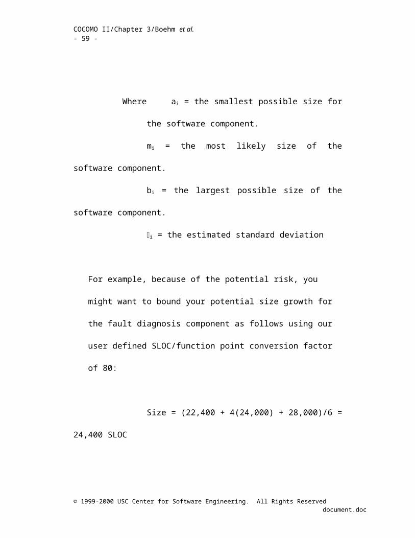
COCOMO II/Chapter 3/Boehm et al. - 59 -
Using the application point procedure, the following sizes shown in Table
3-18 were derived based on the elements in Table 3-17.
[Insert Table 3.18]
There is a pool of five senior developers that could be made available to
work on the project, but they are also critical to ongoing projects. They would
collectively and individually rate as "high" on the developer ICASE experience
scale. Also, the ICASE toolset rates “high”. Can the prototype be done in the
required 6 weeks, and how many developers should be devoted to the project?
With a “high” productivity of 25 NAP/PM per the application point
procedure in section 5.1, the estimated prototype effort for 136.3 NAP would be:
PM = NAP/PROD = 136.3/25 = 5.45 PM (or 23.6 person-weeks).
This would require an average of (23.5 person-weeks/6 weeks)=3.9 full-
time personnel for the six week period, or 4 of the 5 available developers.
3.3.3 Breadboard System (Elaboration Phase)
© 1999-2000 USC Center for Software Engineering. All Rights Reserved document.doc

COCOMO II/Chapter 3/Boehm et al. - 60 -
The breadboard system is planned to demonstrate a defined software
architecture with advancements in newly developed hardware. It will be
extensively tested operationally before committing to final development. There
are still a good number of unknowns at this stage. Though the development
platform is chosen, little is known about the final component sizes, the personnel
available, the real-time performance of the new architecture, or the process to be
used in the final development (there are several major process changes occurring
as part of the software process improvement program). For these reasons, the
coarse-grained Early Design model will be used.
At this relatively early project stage, the amount of functionality can be
quantified easier than the lines of code. But since different designers handle the
different components, the estimated sizes are a mixed bag of function points and
SLOC. The unadjusted function points will be converted to SLOC for the
COCOMO equations.
The breadboard development will also be used as a vehicle to collect cost-
related data. The automated translation productivity will be measured for the
FORTRAN to Ada re-engineered portion in the Radar Item Processing software.
Additionally, the object-oriented development in the Radar Item Processing and
Radar Database will be used to get representative sizes on objects. This object
data will be used later in full development to convert the remaining objects to be
developed to lines of code for the post-architecture model.
© 1999-2000 USC Center for Software Engineering. All Rights Reserved document.doc

COCOMO II/Chapter 3/Boehm et al. - 61 -
Megaspace has also decided to implement Integrated Product Teams for
the breadboard and full development. There is required reuse across a whole
product line, the personnel are highly capable, but some of the staff is new to the
domain. Tables 3-18 and 3-14 list the scale driver and cost driver ratings with
associated rationale for the breadboard development.
[Insert Table 3.19]
[Insert Table 3.20]
Table 3-21 shows the size calculations for the breadboard development. It
implements the equivalent size calculations described in Chapter 2. Note that a
component can be broken up based on sub-components, different languages,
and/or grouped by different origins (e.g. new, reused, modified or COTS). The
data in Table 3-21 is aggregated on a component basis. The granularity of the
components will be dictated by the project nature. In general, finer breakdown is
advantageous since it leads to better system understanding. The same methods of
rolling up sizes apply in all cases. Note also that the reuse parameter heuristics in
Table 2.8 have been followed (e.g. “reused code” implies DM=0, CM=0, and
SU/UNFM don't apply). Any software retained as is from the prototype is
© 1999-2000 USC Center for Software Engineering. All Rights Reserved document.doc
COCOMO II/Chapter 3/Boehm et al. - 62 -
considered reused. Software changed from the prototype is considered
“modified”.
[Insert Table 3.21]
Some qualifications are necessary regarding the COTS data. Source code
sizes for COTS are often unknowable since packages are insular, and source is not
even provided in many cases. COTS size is also irrelevant in situations when its
usage is essentially transparent. Often only a small part of the package is used as
well. It is the interfaces that matter, and the development of glue code that
requires effort. COTS must be handled in some fashion until the COCOTS model
is fully available (see Chapter 5, section 5.4).
In this application, there is access to the COTS source code. It has been
integrated with the rest of the application and downloaded into the embedded
processors. Thus there is complete visibility into the source code, including how
to modify it.
Though the Early Design model can handle function points, the sizes in
Table 3-21 are summarized in SLOC. The sizes of Radar Item Processing and
Radar Database have been converted from function points as follows using the
conversions in Table 2.4 for Ada 95.
© 1999-2000 USC Center for Software Engineering. All Rights Reserved document.doc
COCOMO II/Chapter 3/Boehm et al. - 63 -
Radar Item Processing: 390 FP * 49 SLOC/FP = 19,110 SLOC
Radar Database: 128 FP * 49 SLOC/FP = 6,272 SLOC.
In this and subsequent examples, requirements evolution and volatility
(REVL) is assumed constant within a component regardless of whether it’s new
or adapted (although it doesn’t always have to be the case). The last column in
the table marked “Equivalent Size” adjusts for the adaptation parameters and adds
on the specified percentage of requirements evolution and volatility. This is the
size used in the COCOMO estimating equations.
Equivalent size calculations are not performed for automatically translated
code. The overall effort is calculated with Equation 2.11, with a separate term for
automatic translation. The effort for translating Fortran into Ada is done
separately per Equation 2.6, where the translation effort is added to the standard
COCOMO effort equation. At this stage, automatic translation productivity is not
well-known, so 800 SLOC/person-month will be used based on preliminary data
from another program. Another assumption is that 90% of the Radar Item
Processing 25,450 SLOC can be automatically translated, based on vendor
information. The remaining 10% is developed anew, and shows up as part of the
19,100 new SLOC for the component. Using the 25,450 SLOC portion that will
be converted to Ada, the automatic translation effort alone is:
PMM = ASLOC (AT/100) / ATPROD
© 1999-2000 USC Center for Software Engineering. All Rights Reserved document.doc
COCOMO II/Chapter 3/Boehm et al. - 64 -
= 25,450 ASLOC * (.9) / (800 SLOC/person-month)
= 28.6 person-months.
Putting the equivalent size from Table 3-21 into the Early Design model
effort formula (equation 2.11) gives:
PM = (show formula) = 395.7 person-months.
The overall effort is then 28.6 plus 395.7 = 424.4 person-months.
The overall schedule is calculated with equation 2.14, not including the
separate automated translation effort which is assumed off the critical path:
TDEV = (show formula) = 23.6 months.
Figure 3-10 shows the USC COCOMO output for this estimate using the
Early Design model. In this case since the cost drivers apply to all components,
the overall equivalent size for the system was input. It already takes into account
the adaptation and REVL adjustments calculated in Table 3-21. A user does not
© 1999-2000 USC Center for Software Engineering. All Rights Reserved document.doc

COCOMO II/Chapter 3/Boehm et al. - 65 -
need to produce a separate table like that in Table 3-21, since it was for
demonstration only. Normally a cost estimation tool will do the size calculations.
[Insert Figure 3.10]
3.3.4 Full Development - Top Level Estimate
Several refinements to the system were required after test and evaluation
of the breadboard system. The re-engineered Radar Item Processing software
required modifications to some real-time filtering modules, since the automatic
translation didn't optimize for real-time performance. Additionally, the
breadboard hardware performed slightly differently than anticipated, so the radar
control software required some tweaking. A group of mostly experienced
personnel has also been transferred to the project.
As previously mentioned, the breadboard experience was also used to
refine some cost assumptions. The productivity of automatic translation
measured in the breadboard will be used to estimate the translation effort in the
full development. Also, the subset of the object-oriented design developed in the
breadboard was used to quantify the sizes of objects in lines of code. The
remaining objects to be developed are converted to lines of code based on
representative object samples measured in the breadboard. It is important to note
© 1999-2000 USC Center for Software Engineering. All Rights Reserved document.doc

COCOMO II/Chapter 3/Boehm et al. - 66 -
that COCOMO II may eventually be formulated based on object-oriented size
measures such as those in the Unified Modeling Language (UML), and those in
object-oriented languages such as Ada 95, C++ and Java.
This last exercise for full development of the ARS will introduce the
historical ratings profile which is used to assist in rating new projects. One of the
difficulties of implementing COCOMO or other cost models is rating cost drivers
in a consistent and objective fashion across an organization. To support
consistent rating of cost drivers among individuals and projects, a cost driver
ratings profile has been developed. The ratings profile as part of a defined cost
estimation process is consistent with SEI CMM guidelines, and is adjunct to other
calibration data.
The cost driver ratings profile is a graphical depiction of the objective
rating criteria and historical ratings from past projects to be used as a reference
baseline when performing estimates. It is used in conjunction with a COCOMO
estimation tool, so that new or proposed projects can be easily gauged against past
ones in an objective manner. Since an estimator needs to work closely with
project engineers and architects to assess cost drivers, it is generally easier for
project personnel who aren’t COCOMO experts to perform relative assessments
against known projects rather than starting with a blank slate.
A wideband Delphi technique [Boehm 81] is used along with the ratings
profile to reach consensus in the organization in order to determine the project’s
© 1999-2000 USC Center for Software Engineering. All Rights Reserved document.doc

COCOMO II/Chapter 3/Boehm et al. - 67 -
cost driver ratings. There may often be separate profiles for different product
lines.
Figure 3-11 shows the first two pages of an example Megaspace ratings
profile (see the CD-ROM for an entire profile). The following project description
is used in conjunction with the profile to estimate the effort and schedule for the
final cycle of development. First we perform a top level estimate which assumes
all components are rated the same.
[Insert Figure 3.11]
The project is similar to the historical project BST-2 (another major upgrade
to an existing system) except for the following differences:
Most of the same staff will develop the system, except they now have two
more years of experience relative to their BST-2 ratings. Despite the new
hardware, assume that the platform appears very similar to the one used in
BST-2.
The spiral development approach has reduced the number of unspecified
interfaces and remaining major risks to only 10%.
© 1999-2000 USC Center for Software Engineering. All Rights Reserved document.doc

COCOMO II/Chapter 3/Boehm et al. - 68 -
There will be a new operating system used for development. In the past year
of its use, there have been 5 major changes to the OS.
The project has also invested in an integrated software engineering
environment that supports all life-cycle phases, and is mandated for use by the
developers.
The database size proportion will be very similar to the MINK project.
Process improvement activities have resulted in an SEI CMM Level 3 rating.
Same required reuseability as the breadboard development, i.e. it must be
designed for reuse.
Using the above descriptions in conjunction with the BST-2 and MINK
ratings, the scale and cost driver ratings in Tables 3-22 and 3-23 are obtained.
[Insert Table 3.22]
© 1999-2000 USC Center for Software Engineering. All Rights Reserved document.doc

COCOMO II/Chapter 3/Boehm et al. - 69 -
[Insert Table 3.23]
For the Radar Unit Control component, the estimate of new code
development is 3,215 SLOC of Ada, with 500 SLOC being modified from the
breadboard baseline. It is estimated that about 30% of the design will have to be
modified with considerable test and evaluation of the modified components to
assess them. It is thought that the code to be modified is fairly well-structured,
but has little correlation between program and application views. There is a
medium amount of documentation associated with the code.
The Radar Item Processing software can be sub-divided into new,
modified from the breadboard and automatically translated. In the modified
portion of 11,500 SLOC, only 5% of the design needs to be changed, 14% of the
code will be modified, and 100% re-testing will be required. The breadboard
development produced excellent documentation for the object-oriented Ada 95
portions. The design and code was made to be reused and requires no assessment.
An estimated 13,715 SLOC will be developed new.
The Radar Database component will have 12,200 new SLOC, and the rest
is reused.
The Display Manager software requires 15,400 new SLOC, and the rest
will be reused from the breadboard.
© 1999-2000 USC Center for Software Engineering. All Rights Reserved document.doc

COCOMO II/Chapter 3/Boehm et al. - 70 -
The Display Console software is estimated as 13,200 new SLOC and very
little modification from the breadboard. Only 1,800 SLOC will be modified by
20% for design and code.
Finally, the Built In Test software needs 16,000 SLOC of new software,
and the existing base is completely reused. It automatically diagnoses faults and
identifies problems at the hardware replaceable unit level. It also supports fault
tolerance since the system must be highly reliable.
One half of the staff was present during the breadboard development, and
the other half is new. The average familiarity with the existing software is
somewhat familiar (assume this holds for all components). For all modified
software, assume the same software understanding parameters hold as for Radar
Unit Control.
Table 3-24 shows the size calculations based on these descriptions. Since
there is more project detail known compared to the breadboard system, the
component data is more detailed than the breadboard estimate. Note that the
COTS code is treated as reused code. The equivalent size calculations are shown
to illustrate the method, since most COCOMO tools automate the calculations
based on input reuse parameters.
Unless stated otherwise, the Assessment and Assimilation increment is 0
for reused code, and 2 for modified code.
© 1999-2000 USC Center for Software Engineering. All Rights Reserved document.doc

COCOMO II/Chapter 3/Boehm et al. - 71 -
[Insert Table 3.24]
As in the breadboard system, equivalent size calculations are not
performed for automatically translated code. For the ARS, automatic translation
productivity was measured during the breadboard development as 1,150
SLOC/person-month. It was also found that only 75% of the original radar item
processing code could be successfully translated by tools. The remaining portion
to be converted to Ada is 58,320 SLOC. The automatic translation effort alone is:
PMM = ASLOC (AT/100) / ATPROD
= 58,320 ASLOC * (.75)/1,150 SLOC/person-month)
= 38.0 person-months.
Note that schedule constraint effects are not applied to the automatic
translation effort. The remaining effort for the rest of the system is estimated as:
PM = (show formula) = 459 person-months.
The overall effort is then 459 + 38 = 497 person-months.
The overall schedule is calculated with equation 2.14 (again excluding the
automated translation effort):
© 1999-2000 USC Center for Software Engineering. All Rights Reserved document.doc
COCOMO II/Chapter 3/Boehm et al. - 72 -
TDEV = (show formula) = 16.8 months.
Even though the effort is larger than the breadboard development, the
schedule time is less.
Figure 3-12 shows the USC COCOMO output screen for this case, and
Figure 3-13 shows the cost driver ratings. Since this was a top level estimate, the
system was treated as a single component with the total equivalent SLOC.
Alternatively, component size information could have been input with each
component having the same cost driver ratings.
[Insert Figure 3.12]
[Insert Figure 3.13]
3.3.5 Full Development - Detailed Component Estimate
The previous exercise demonstrated a top-level estimate, whereby all the
components were treated in aggregate. This exercise will instead account for
© 1999-2000 USC Center for Software Engineering. All Rights Reserved document.doc
COCOMO II/Chapter 3/Boehm et al. - 73 -
differences in the component cost driver ratings. The scale drivers stay the same
since they apply to the project as a whole.
Tables 3-25 through 3-30 show the detailed cost driver ratings and
rationale that differ from the top-level estimate. Most of the component cost
drivers remain the same as the aggregate ones, so only the changed ones are listed
for convenience1. Differences between components are due primarily to different
functional specifications, different teams, or varying development environments.
For example, the Built In Test TOOL rating is lower since standard tools don't
cover the more complex and low-level hardware testing environment. The
development and testing require more primitive operations.
[Insert Table 3.25]
[Insert Table 3.26]
[Insert Table 3.27]
[Insert Table 3.28]
[Insert Table 3.29]
1 Some estimation tools provide hierarchical inheritance of default cost driver settings to minimize user inputs in such a situation.
© 1999-2000 USC Center for Software Engineering. All Rights Reserved document.doc
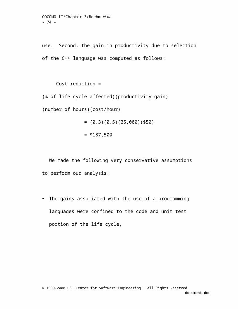
COCOMO II/Chapter 3/Boehm et al. - 74 -
[Insert Table 3.30]
As in the previous top level estimate, automatic translation effort is
calculated alone to be 38 person-months. Using the detailed component data, the
remaining effort for the rest of the system is estimated as:
PM = (show formula) = 620 person-months.
The overall effort is then 620 + 38 = 658 person-months.
The overall schedule is calculated with equation 2.14:
TDEV = (show formula) = 17.9 months.
Figure 3-14 shows the USC COCOMO output. The last column labeled “RISK”
shows a top-level assessment of project risk based on cost driver ratings. The Expert
COCOMO risk assessment scheme is overviewed in chapter 5 (Emerging Extensions),
section 5.7 and detailed in [Madachy 97].
[Insert Figure 3.14]
© 1999-2000 USC Center for Software Engineering. All Rights Reserved document.doc

COCOMO II/Chapter 3/Boehm et al. - 75 -
Refining an estimate in detail such as this serves to rethink assumptions
and usually converges toward a better estimate. In this case, a more detailed look
produces an estimate for 161 PM more effort and an extra month of schedule time
compared to the top level estimate. The extra detail is also essential for large-
project planning and control instruments such as Work Breakdown Structures and
earned-value tracking systems.
3.3.6 Incremental Development Example
This section applies COCOMO II to incremental development, which is a
commonly used lifecycle approach. The formulas for incremental COCOMO
used in this example are described in Appendix B. This example separates the
previous single-shot development shown in Section 3.3.5 into three time-phased
increments, or individually delivered “builds” of software.
Incremental development reduces risk by providing reduced-scale
increments of increasing functionality. It tends to create a flatter staffing profile
compared to a single-shot waterfall approach, but increases schedule time
somewhat [SEE pp. 41-44]. The development process described here is also
called an incremental waterfall, since requirements and preliminary design are
conducted first for all increments before individual increments are developed.
Implementation of separate increments is carefully scheduled in time, and
© 1999-2000 USC Center for Software Engineering. All Rights Reserved document.doc

COCOMO II/Chapter 3/Boehm et al. - 76 -
normally there is some parallel work being done on more than one increment
simultaneously.
The USC COCOMO tool used thus far is based on waterfall lifecycle
activities (a single sequence of requirements, design, code/unit test, integration
and testing) with no explicit utilities for estimating multiple increments. In order
to estimate incremental development with USC COCOMO, several runs would be
made with manual adjustments to effort and schedule, and then the results would
have to be combined. The commercial tool Costar provides a comprehensive
implementation of incremental COCOMO consistent with the Appendix B
definition, and will be used in this example.
When planning incremental builds, deciding which functions to deliver when
depends on specific project factors. In this case of the radar system, the following
constraints will guide the phasing of incremental functionality:
A large portion of the Display software is wanted early for user interface and
scenario evaluation, and the remainder will be split among the later two
builds. Nearly the entire set of graphic primitives is needed first to enable the
sophisticated displays, and for general performance testing of the graphics
engine and human-machine interface.
© 1999-2000 USC Center for Software Engineering. All Rights Reserved document.doc

COCOMO II/Chapter 3/Boehm et al. - 77 -
There is an urgent need for a subset of the Radar Item Processing and Radar
Database software dedicated to specific vehicles involved in a current military
situation, so it’s critical that this software is delivered in the first increment.
To enable quickest delivery of this capability, all other radar items will be
deferred until later builds.
Most of the Radar Unit Control functionality will be present in the first
increment, since the interface and basic operating parameters are well-known
from previous experience. However, the radar hardware is new and there are
some new capabilities planned for the latter two increments.
The Built In Test software requires the final radar item hardware for most of
its operations, so only a shell process will exist until the final build when the
hardware will be ready.
Given these constraints, the following portions of software are planned per
increment:
Increment 1
50% of Display Manager
80% of Display Console
© 1999-2000 USC Center for Software Engineering. All Rights Reserved document.doc
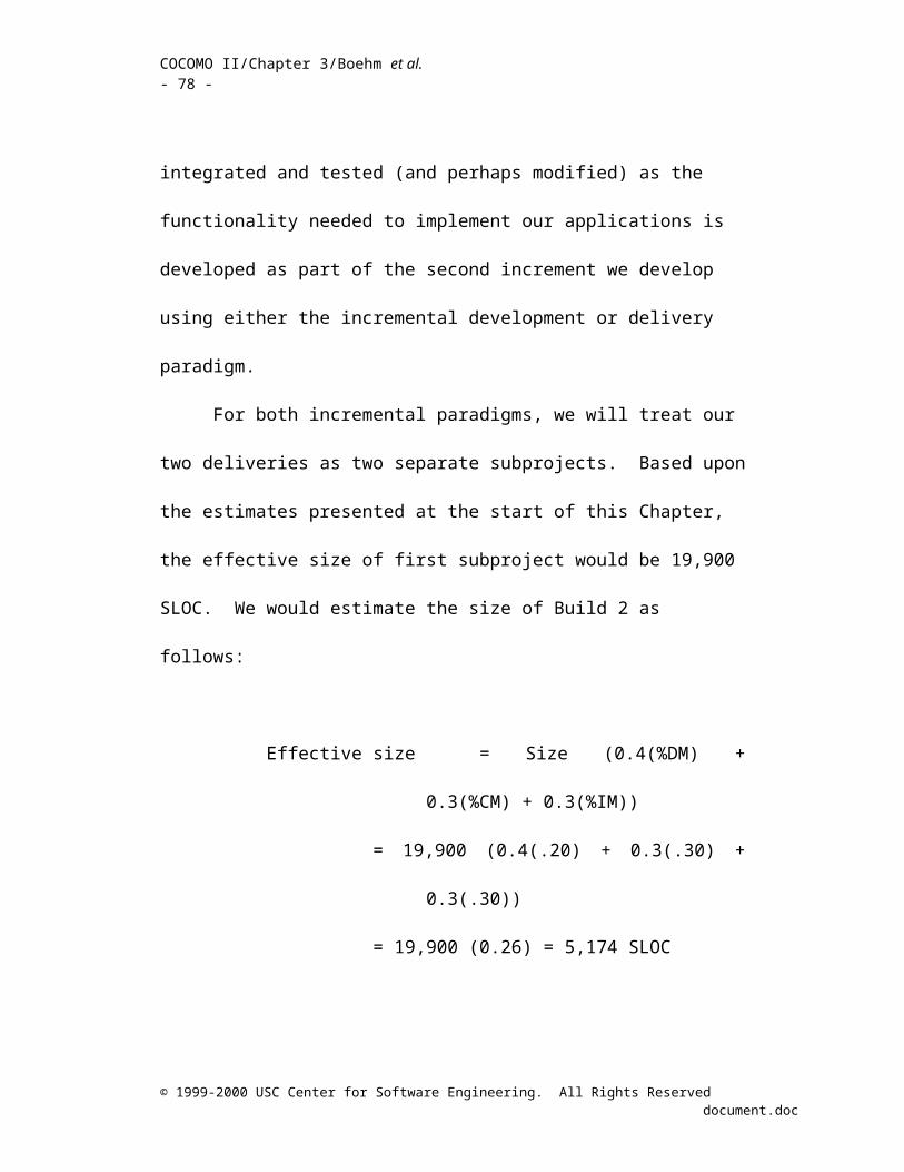
COCOMO II/Chapter 3/Boehm et al. - 78 -
25% of Radar Item Processing and Radar Database
5% of Built In Test
70% of Radar Unit Control
Increment 2
25% of Display Manager
15% of Display Console
45% of Radar Item Processing and Radar Database
10% of Built In Test
15% of Radar Unit Control
Increment 3
25% of Display Manager
5% of Display Console
30% of Radar Item Processing and Radar Database
85% of Built In Test
15% of Radar Unit Control
Increment Volatility
There is a nominal amount of requirements evolution and volatility
expected. Specifications for the new radar items are volatile since intelligence
information is still being gathered, so 30% requirements evolution and volatility is
© 1999-2000 USC Center for Software Engineering. All Rights Reserved document.doc

COCOMO II/Chapter 3/Boehm et al. - 79 -
expected for Increment 1 in the Radar Item Processing and Radar Database areas.
The requirements evolution and volatility in these areas is estimated to be only
20% and 15% for the last increments. Experience with Increment 1 displays will
likely cause a little volatility during the latter increments, so 10% will be assumed
for the latter increments for both Display Manager and Display Console. Only
10% requirements evolution and volatility of the first increment of Radar Unit
Control is expected, but 20% for the last two since those represent untried
capabilities. Most of the changes to Built In Test will occur after field testing,
and does not show up in this estimate.
The personnel experience factors will improve slightly between
increments to represent the staff experience gains over the project duration (it’s
expected that most people will stay on the project, and there will be little
attrition). A few of the product factors will also vary between increments for a
given component, to describe the portion of software being worked at different
times.
The chosen incremental phasing model determines the beginning of each
increment relative to predecessor increments. In this example, the starting points
for increments 2 and 3 are the Preliminary Design Walkthrough (PDW)
milestones of the previous increments.
Summary Costar reports are shown in the following figures. Figure 3-15
shows the hierarchical structure of the software components with their respective
© 1999-2000 USC Center for Software Engineering. All Rights Reserved document.doc

COCOMO II/Chapter 3/Boehm et al. - 80 -
equivalent sizes. Note that the three builds serve as hierarchy branches containing
their software components as leaves. One difference with size tables shown
earlier in this section and Figure 3-15 is that a component in Costar has both new
and adapted portions; thus new and modified (or new and reused) parts of a
component are listed as a single component using the Costar tool.
[Insert Figure 3.15]
Figure 3-16 shows increment time phasing assumptions, including the start
point of each increment and any phasing delays. Note the convention that
requirements work is done once for all increments, and that development of the
individual increments includes preliminary design through testing. Figure 3-17
shows increment summary information. There are numerous other screens and
detailed graphical or tabular reports available in Costar.
[Insert Figure 3.16]
[Insert Figure 3.17]
© 1999-2000 USC Center for Software Engineering. All Rights Reserved document.doc