Software and Hardware Techniquesfor Efficient Polymorphic Calls

UNIVERSITY OF CALIFORNIASanta Barbara

A dissertation submitted in partial fulfillmentof the requirements for the degree of

Doctor of Philosophy in Computer Science

by Karel Driesen

Committee in charge:

Professor Urs Hölzle, chairpersonProfessor Klaus SchauserProfessor Anurag AcharyaProfessor Bradley CalderProfessor Trevor Mudge

Professor Yale Patt

Technical Report TRCS99-24June 1999

Acknowledgments“A Ph.D. is a prolonged identity crisis”

Theo D’Hondt [37]

I am deeply indebted to a number of people who supported me in the accomplishment ofthis work. It is impossible to mention all of them within the limits of this page, so I willapologize beforehand to those I forget (you know who you are).

Firstly, my advisor, Urs Hölzle, who not only invited me over to this jewel of the WestCoast, Santa Barbara, but also provided me in ample quantities with the three things a grad-uate student needs: neat toys, time to play with them, and sound advice on how to producesomething useful in the process. Whether it was an ergonomic keyboard tray, a summer RA-ship, or a literature study on conditional branch prediction, Urs anticipated my every needbefore I was even aware of it. He knew when to push me for better performance and whento give me some slack to sort things out. Many times, his constantly positive demeanor keptme going when I felt discouraged. And when I got firmly stuck, he invariably came up witha way out. I feel privileged to have worked so closely with a great mind, who also happensto be a really nice guy. Some debts one cannot hope to pay back.

Secondly, my former advisor, Theo D’Hondt, who supported me in the seven yearspreceding this work, and whose quote graces this page. In the entirely different circum-stances of an underfunded, understaffed and overcrowded department, which he almostsingle-handedly lifted up to its current state (in my humble opinion the foremost academiccenter of object-oriented expertise in Belgium), he exhibited vision, boldness, and a infec-tious love of experimental computer science that influences me to this day. Thanks Theo.

Next, I have to lump together my friends, my family, my tribe. They taught me too manythings to sum up, so I will just try to give a sample: Raimondas Lencevicius, for the Dharmaand perseverance, Ioana Roxana Stanoi, for style, Lara Hassler, for health, Katherine Ford,for building a home, Denis Khotimsky, for scuba diving, Max Ibel, for hacking, RuppertKoch, for mechanics, Shirley Geok-lin Lim, for poetry, Katinka Balthazar, for inspiration,Jennifer West, for physics, Catherine Dibble, for vision, Anne-Lise Vandenborre, for under-standing, Hiroko Takanashi, for eating out, Smitha Vishveshwara, for beach walking,Sylvia A Liseling, for keeping in touch, Bettina Kemme, for shopping, Kevin Murphy, forrunning naked, Gerald Aigner, for down-to-earthness, Michel Tilman, Kris De Volder, JeffBogda, Andrew Duncan, Ralph Keller, Silvie Dieckman, Holger Kienle, for being fun towork with, Karlo Berket, for poker, Michael Schmitt, for winning at poker, Alicia Watt, forgiving hugs, Crina A Vasiliu, for helping out, Jane Carlisle, for saving my life, my parentsJeanne Bleus-Driesen and Frans Driesen, for living, my brothers Willem, Guido and FrankDriesen and my sister, Annie Driesen, for living together, Marlies Bex-Driesen, for caring,Wim Lybaert, for hard-headedness, Wilfried Verachtert, for busyness, Michael Vermeersch,for sarcasm, Luc Hendrix, for fun, Jan Delaet, for rock climbing, Patrick Steyaert, fordaring, Stefan Samyn, for love, peace and respect to the max, Stefan Kuypers, for hospi-tality, Johan Vanderspeeten, for making stuff, Georges Meekers, for guts, Rudi Claes, forbluntness, Peter Muller, for excellence.

And finally, Irene Zafrullah, for love.

ii

Vita

Personalia

Surname: DriesenGiven names: Karel Johannes LodewijkPlace of Birth: Sint-Truiden, Limburg, BelgiumDate of Birth: April 15, 1965Nationality: BelgianAddress: Department of Computer Science

RSL-lab 2122 Engineering IUniversity of California Santa BarbaraCA 93106USA

Telephone: (1-805) 893-4394Fax: (1-805) 893-8553Email: karel@cs.ucsb.eduURL: http://www.cs.ucsb.edu/~karel

Education

Master in Computer Science (VUB Brussels, 1993)Grade: Great DistinctionThesis: “Method Lookup Strategies in Dynamically Typed Object-Oriented ProgrammingLanguages”

Licentiate Computer Science (VUB Brussels, 1987)Grade: Great DistinctionThesis: “Typesystemen in Smalltalk-80” (Type Systems in Smalltalk-80)

Experience

Research assistant (10/1995 - present, Department of Computer Science UCSB Santa-Barbara):Quantitative analysis of polymorphic calls.Indirect branch prediction.

Visiting researcher (10/1994 - 9/1995, Department of Computer Science UCSB Santa-Barbara):Qualitative analysis of message dispatch in object-oriented languages.Optimization of row displacement dispatch tables.

Researcher (12/1993 - 9/1994, Department of Computer Science VUB Brussels):Research project: “Design and Use of Programmable Servers in the Modern Office”Object placing and migration strategies in a distributed OO-system.

Teaching assistant (1/1988 - 11/1993, Department of Computer Science VUB Brussels):Research:- finalization of the Minipas programming environment in Lightspeed Pascal.- analysis of the influence of network topology on generalization performance ofmulti-layered perceptrons (artificial neural networks).

iii

- comparative analysis of message dispatch techniques.- implementation of row displacement compression for dispatch tables.Teaching:- Structure of Computer Programs I- Algorithms and Data Structures I- Algorithms and Data Structures II- Programming Project- Parallel Systems- Analysis and Design- Assistant Thesis Advisor

Elected representative of teaching assistants (1991, Board of directors VUB Brussels)

Elected representative of teaching assistants (1990-1991, Faculty of Sciences board)

Research assistant (10/1987 - 12/1987, Department of Mathematics VUB Brussels):Finalization of the two-year demographic project:“Prognosis of the number of Belgian students until 1995-96”

Programmer (7/1985 - 8/1985, 7/1986 - 9/1986, U-Soft software company based in Hasselt):Machine parts stock management software in UCSD Pascal.Documentation of BancContact server software in COBOL.EBNF to syntax diagrams translation in UCSD Pascal.

Publications

Multi-stage Cascaded Prediction.with Urs HölzleTo appear in the EuroPar’99 Conference Proceedings

The Cascaded Predictor: Economic and Adaptive Branch Target Prediction.with Urs HölzleIn Micro’98 Conference Proceedings, pp. 249-258, Dallas, Texas, December 1998

Accurate Indirect Branch Prediction.with Urs HölzleIn ISCA ‘98 Conference Proceedings, pp. 167-178, Barcelona, July 1998

The Direct Cost of Virtual Function Calls in C++.with Urs HölzleIn OOPSLA ‘96 Conference Proceedings, p. 306-323, San Jose, California,1996. Publishedas SIGPLAN Notices 31(10), October 1996.

Minimizing Row Displacement Dispatch Tables.with Urs HölzleOOPSLA’95 Conference Proceedings: p. 141-155, Austin, Texas, October 1995, Published asSIGPLAN Notices 30(10), October 1995.

iv

Message Dispatch on Modern Computer Architectures.with Urs Hölzle and Jan VitekECOOP ‘95 Conference Proceedings, p. 253-282, Århus, Denmark, August 1995. Publishedas Springer Lecture Notes in Computer Science Vol. 952, Springer-Verlag, Berlin Heidelberg1995

Compressing Sparse Tables using a Genetic Algorithm.Proceedings of the GRONICS’94 Student Conference, Groningen, February 1994.

Selector Table Indexing and Sparse Arrays.OOPSLA ‘93 Conference Proceedings, p. 259-270, Washington, D.C., 1993. Published asSIGPLAN Notices 28(10), September 1993.

Awards

Third place in the 1996 Student Writing Contest of the Society for Technical Communication, Santa-Barbara Chapter, with the white paper “Multiple Dispatch Techniques: a survey.“.

Graduate Division’s Spring 1998 Dissertation Fellowship, University of California, Santa-Barbara

Inventions

“Cascaded Prediction”, Karel Driesen and Hölzle, Patent Pending #09/268483

Reports

Improving Indirect Branch Prediction With Source- and Arity-based Classification and CascadedPrediction.with Urs HölzleTechnical Report TRCS98-07, Department of Computer Science, University of CaliforniaSanta-Barbara, March 15, 1998

Limits of Indirect Branch Prediction.with Urs HölzleTechnical Report TRCS97-10, Department of Computer Science, University of CaliforniaSanta-Barbara, June 25, 1997

Multiple Dispatch Techniques: a survey.White paper, Santa-Barbara, 1996.

Method Lookup Strategies in Dynamically-Typed Object-Oriented Programming Languages.Master’s Thesis, Free Brussels University (VUB) 1993.

Prognosis of the number of Belgian students until 1995-96with Franz Bingen and Carlos SiauInternal publication Free Brussels University (VUB) 1988

Typesystemen in Smalltalk-80.(Type Systems in Smalltalk-80)Licentiate Thesis, Free Brussels University (VUB) 1987

v

Abstract

Object-oriented code looks different from procedural code. The main difference is theincreased frequency ofpolymorphic calls. A polymorphic call looks like a procedural call,but where a procedural call has only one possible target subroutine, a polymorphic call canresult in the execution of one of several different subroutines. The choice is made at runtime, and depends on the type of the receiving object (the first argument). Polymorphic callsenable the construction of clean, modular code design. They allow the programmer toinvoke operations on an object without knowing its exact type in advance.

This flexibility incurs an overhead: in general, polymorphic calls must be resolved at runtime. The overhead of this run time polymorphic call resolution can lead a programmer tosacrifice clarity of design for more efficient code, by replacing instances of polymorphiccalls by several single-target procedural calls, removing run time polymorphism. This prac-tice typically leads to a more rigid program structure and code duplication, increasing theshort term effort required to build a functional prototype, and the long term effort of main-taining and adapting a program to changing needs.

We study techniques to minimize the run-time cost of polymorphic calls. In the softwaredomain, we minimize the memory overhead of table based implementations (messagedispatch tables), which are most efficient in terms of number of instructions executed. In thehardware domain, we reduce the cycle cost of these instructions through indirect branchprediction. For reasonable transistor budgets, hit rates of more than 95% can be achieved.As a result, only one out of twenty polymorphic calls incurs significant cost at run time.

Design of clear, maintainable and reusable code, as enabled by object-oriented technology,can thereby become less restrained by efficiency considerations. Only in very time-criticalprogram segments should the programmer avoid the use of polymorphism. In other words,object-oriented code can become the norm rather than the exception. From our own expe-rience in building software architectures, we consider this a Good Thing.

vi

Table of Contents

1 Introduction .....................................................................................................................11.1 Problem statement ....................................................................................................21.2 Background and motivation .....................................................................................21.2.1 Inheritance .........................................................................................................41.2.1.1 Subtyping ...................................................................................................41.2.1.2 Subclassing ................................................................................................41.3 Contributions ............................................................................................................51.4 Overview ..................................................................................................................8

2 Polymorphic calls ............................................................................................................92.1 Basic construct .........................................................................................................92.2 Polymorphic calls in procedural languages ...........................................................102.3 Object-oriented message dispatch ..........................................................................102.3.1 Static vs. dynamic typing ................................................................................112.3.2 Single vs. multiple inheritance ........................................................................122.3.3 Single vs. multiple dispatch ............................................................................132.3.4 Predicate dispatch ...........................................................................................14

3 Software techniques for efficient polymorphic calls .....................................................153.1 Basic message dispatch in object-oriented languages ............................................153.1.1 Influence of dynamic typing ...........................................................................163.1.2 Influence of multiple inheritance ....................................................................163.2 Dynamic techniques ...............................................................................................173.2.1 Global lookup caches (LC) .............................................................................183.2.2 Inline caches (IC) ............................................................................................183.2.3 Polymorphic inline caching (PIC) ..................................................................193.3 Static techniques ....................................................................................................203.3.1 Selector table indexing (STI) ..........................................................................203.3.2 Virtual function tables (VTBL) .......................................................................213.3.3 Selector coloring (SC) .....................................................................................223.3.4 Row displacement (RD) ..................................................................................233.3.5 Compact selector-indexed dispatch tables (CT) .............................................243.4 Memory cost ..........................................................................................................263.4.1 Single inheritance cost ....................................................................................263.4.2 Multiple inheritance cost .................................................................................283.5 Programming environment aspects ........................................................................293.6 Summary ................................................................................................................30

4 Row displacement compression ....................................................................................314.1 Class-based row displacement ...............................................................................324.2 Selector-based row displacement ...........................................................................334.2.1 Distribution of row sizes .................................................................................344.2.2 Fitting order ....................................................................................................36

vii

4.2.3 Class numbering for single inheritance .......................................................... 364.2.4 Class numbering for multiple inheritance ...................................................... 374.2.5 Summary ........................................................................................................ 394.3 Compression results ............................................................................................... 404.3.1 Methodology .................................................................................................. 404.3.2 Samples .......................................................................................................... 414.3.3 Compression results ....................................................................................... 414.4 Optimizing table compression speed ..................................................................... 434.4.1 Compression algorithms ................................................................................. 434.4.2 Compression speed ......................................................................................... 464.5 Applicability to interactive programming environments ....................................... 474.6 Summary ................................................................................................................ 47

5 Analysis of dispatch sequences on modern processor architectures ............................ 495.1 Parameters influencing performance ..................................................................... 495.2 Dispatch cost calculation ....................................................................................... 515.2.1 VTBL call code scheduling ............................................................................ 515.2.2 Other techniques ............................................................................................. 525.3 Cost of dynamic typing and multiple inheritance .................................................. 545.4 Influence of processor implementation ................................................................. 555.5 Limitations ............................................................................................................. 575.6 Summary ................................................................................................................ 58

6 Measurement of virtual function call overhead on modern processors ........................ 616.1 Virtual function tables and the thunk variant ......................................................... 616.2 Superscalar processors ........................................................................................... 626.2.1 BTB branch prediction ................................................................................... 646.2.2 Advanced superscalar execution .................................................................... 646.2.3 Co-scheduling of application code ................................................................. 656.2.4 Summary ........................................................................................................ 656.3 Method ................................................................................................................... 666.3.1 Simulation scheme ......................................................................................... 666.3.2 Benchmarks .................................................................................................... 686.3.3 Processors ....................................................................................................... 696.4 Results ................................................................................................................... 716.4.1 Instructions and cycles ................................................................................... 716.4.2 Thunks ............................................................................................................ 726.4.3 Generalization to other processors ................................................................. 736.4.4 Influence of branch penalty ............................................................................ 756.4.5 Influence of branch prediction ........................................................................ 766.4.6 Influence of load latency ................................................................................ 816.4.7 Influence of issue width .................................................................................. 816.4.8 Cost per dispatch ............................................................................................ 826.5 Discussion .............................................................................................................. 846.6 Summary ................................................................................................................ 85

viii

7 Hardware techniques for efficient polymorphic calls ................................................... 877.1 Software vs. hardware prediction .......................................................................... 877.2 Hardware indirect branch prediction ..................................................................... 897.3 Indirect branch frequency ...................................................................................... 897.3.1 Benchmark overview ...................................................................................... 897.3.2 Branch frequency measurements .................................................................... 917.4 Experimental setup ................................................................................................ 937.5 Problem statement ................................................................................................. 93

8 Basic indirect branch predictors ................................................................................... 958.1 Branch target buffer ............................................................................................... 958.1.1 2-bit counter update rule ................................................................................ 958.2 Two-level predictor ................................................................................................ 968.2.1 First level: history pattern ............................................................................... 978.2.2 Second level: history table sharing ................................................................. 998.2.3 Path length .................................................................................................... 1008.3 History buffers ..................................................................................................... 1018.3.1 Trace information ......................................................................................... 1018.3.2 History pattern compression ......................................................................... 1018.3.2.1 Target pattern projection ....................................................................... 1018.3.2.2 Address folding ..................................................................................... 1038.4 History tables ....................................................................................................... 1038.4.1 Capacity misses ............................................................................................ 1038.4.2 Conflict misses ............................................................................................. 1048.4.2.1 Interleaving ........................................................................................... 1058.4.2.2 Associativity .......................................................................................... 1078.5 Summary .............................................................................................................. 109

9 Hybrid indirect branch predictors ............................................................................... 1119.1 Hybrid prediction ................................................................................................. 1119.1.1 Components .................................................................................................. 1119.1.2 Meta prediction ............................................................................................ 1129.2 Branch classification ............................................................................................ 1139.2.1 Opcode-based classification ......................................................................... 1139.2.2 Arity-based classification ............................................................................. 1169.2.3 Discussion .................................................................................................... 1199.3 Dual-path hybrid prediction ................................................................................ 1209.3.1 Meta prediction ............................................................................................ 1209.3.2 Component predictors .................................................................................. 1219.3.3 Results .......................................................................................................... 1229.4 Cascaded prediction ............................................................................................. 1249.4.1 Metaprediction ............................................................................................. 1249.4.1.1 Table update filtering ............................................................................. 1259.4.2 Cascaded prediction with a BTB as first stage ............................................. 1259.4.2.1 Strict filters ............................................................................................ 126

ix

9.4.2.2 Leaky filters ........................................................................................... 1279.4.2.3 Results ................................................................................................... 1289.4.3 Multi-stage cascaded prediction ................................................................... 1329.4.3.1 Predictor components ............................................................................ 1329.4.3.2 Ideal predictors ...................................................................................... 1349.4.3.3 Practical predictors ................................................................................ 1369.4.3.4 Results ................................................................................................... 1389.4.3.5 Detailed data ......................................................................................... 1409.4.4 Conclusions .................................................................................................. 1439.5 Summary .............................................................................................................. 143

10 Related work ............................................................................................................... 14510.1 Software techniques ............................................................................................. 14510.1.1 Code rewriting optimization ......................................................................... 14510.1.2 Message dispatch techniques ....................................................................... 14610.1.3 Multiple dispatch techniques ........................................................................ 14710.1.4 Dispatch table compression .......................................................................... 14810.2 Hardware techniques ........................................................................................... 15010.2.1 Indirect branch prediction ............................................................................ 15010.2.2 Prediction architectures ................................................................................ 15110.2.2.1 Basic prediction ..................................................................................... 15110.2.2.2 Hybrid prediction .................................................................................. 152

11 Future work and open problems ................................................................................. 15511.1 Software techniques ............................................................................................. 15511.1.1 Inline caching with fast subtype tests ........................................................... 15511.1.2 Global caching with history ......................................................................... 15511.2 The software-hardware interface ......................................................................... 15611.2.1 Measuring cycle cost of software techniques on superscalar processors ..... 15611.2.2 Benchmarking Java ...................................................................................... 15611.2.3 Influence of code-rewriting techniques on indirect branch population ........ 15611.2.4 Feedback from predictor hardware to code-rewriting techniques ................ 15711.3 Exploring different applications for hardware-based prediction ......................... 15811.4 Algorithms ........................................................................................................... 15911.5 Misprediction rate as a program complexity metric ............................................ 159

12 Conclusions ................................................................................................................ 161

13 Glossary ...................................................................................................................... 163

14 References .................................................................................................................. 165

x

List of figures

Figure 1. Fragment of the UCSB webpagewww.ucsb.edu (Author:Joseph Boisse)............ 2Figure 2. Object types (classes) and polymorphic calls ....................................................... 3Figure 3. Subtype hierarchy ................................................................................................. 4Figure 4. Subclass hierarchy................................................................................................. 5Figure 5. Single inheritance with multiple root classes...................................................... 11Figure 6. Multiple inheritance ............................................................................................ 12Figure 7. Class hierarchy with corresponding dispatch tables ........................................... 15Figure 8. Memory layout of objects in the case of multiple inheritance............................ 17Figure 9. Global lookup cache............................................................................................ 18Figure 10. Inline cache ......................................................................................................... 19Figure 11. Polymorphic inline cache.................................................................................... 19Figure 12. Selector Table Indexing ...................................................................................... 20Figure 13. VTBL dispatch tables and method call code. ..................................................... 21Figure 14. Selector coloring tables, method call code, and method prologue...................... 22Figure 15. Row displacement tables, method call code, and method prologue ................... 23Figure 16. Construction of Compact Tables......................................................................... 24Figure 17. CT dispatch code................................................................................................. 25Figure 18. Space overhead for the Smalltalk system ........................................................... 27Figure 19. Class-based row displacement tables.................................................................. 32Figure 20. Selector-based row displacement tables ............................................................. 33Figure 21. Table size distribution forMagnitude(18 classes, 240 selectors). ..................... 34Figure 22. Alphabetic and depth-first class numbers ........................................................... 37Figure 23. Magnitude: selector-based tables ........................................................................ 38Figure 24. Multiple inheritance class numbering................................................................. 39Figure 25. One-entry row fitting .......................................................................................... 45Figure 26. VTBL-MI schedules and dependencies, cycle counts and assembly code. ........ 52Figure 27. Performance of dispatch mechanisms (single inheritance)................................. 54Figure 28. Influence of branch misprediction penalty on dispatch cost in P97 ................... 56Figure 29. Instruction sequence for VFT dispatch ............................................................... 61Figure 30. Thunk virtual function tables .............................................................................. 62Figure 31. Simplified organization of a superscalar CPU.................................................... 63Figure 32. Overview of experimental setup ......................................................................... 67Figure 33. Direct cost of standard VFT dispatch (unmodified benchmarks) ....................... 71Figure 34. Direct cost of standard VFT dispatch (all-virtual benchmarks).......................... 72Figure 35. Cycle cost of standard and thunk variants (unmodified benchmarks) ................ 73Figure 36. Cycle cost of standard and thunk variants (all-virtual benchmarks)................... 74Figure 37. Dispatch overhead in P96 vs. P96-noBTB and P96-Pro..................................... 75Figure 38. Overhead in cycles for varying branch penalties ............................................... 76Figure 39. Overhead in % of execution time for varying branch penalties.......................... 77Figure 40. Overhead in cycles for varying Branch Target Buffer sizes............................... 78Figure 41. Overhead in% of execution time for varying BTB sizes .................................... 79

xi

Figure 42. Indirect branch prediction ratio as a function of BTB size..................................80Figure 43. Overhead in % of execution time for varying issue widths.................................82Figure 44. Cycles per dispatch under various BTB prediction regimes ...............................83Figure 45. Average execution distance between indirect branches ......................................92Figure 46. Average distance between executions of the same branch..................................93Figure 47. Experimental setup ..............................................................................................94Figure 48. Branch target Buffer ............................................................................................95Figure 49. Indirect branch misprediction rates for an unconstrained BTB...........................96Figure 50. Two-level branch prediction................................................................................96Figure 51. History pattern sharing ........................................................................................97Figure 52. Influence of history sharing for path length p=8, per-branch entries ..................98Figure 53. History Table sharing ..........................................................................................99Figure 54. Influence of history table sharing with a global history pattern. .........................99Figure 55. Two level branch prediction ..............................................................................100Figure 56. Misprediction rates per path length (global history, per-address table entries).100Figure 57. Limited Precision misprediction rates. ..............................................................102Figure 58. AVG of limited size fully-associative misprediction ratios ..............................104Figure 59. Misprediction rates using concatenation (4K entries) .......................................105Figure 60. Concatenation and interleaving of target address bits .......................................106Figure 61. Misprediction rates using reverse interleaving (4K-entries) .............................106Figure 62. Interleaving schemes .........................................................................................107Figure 63. AVG misprediction rates for various table sizes and associativity ...................108Figure 64. Basic component predictor. ...............................................................................112Figure 65. Classifying hybrid predictor with shared history table......................................113Figure 66. Misprediction rates per opcode-based branch class ..........................................114Figure 67. Misprediction rates for opcode-based classifying predictors ............................115Figure 68. Misprediction rates per arity-based branch class...............................................117Figure 69. Misprediction rates for arity-based classifying predictors ................................118Figure 70. Dual-path hybrid predictor scheme ...................................................................120Figure 71. Prediction hit rates for dual-path hybrid predictors...........................................121Figure 72. Misprediction rates per table size, associativity and predictor type ..................122Figure 73. Cascaded predictor scheme ...............................................................................124Figure 74. Misprediction rates for a cascaded predictor with strict filter ...........................127Figure 75. Misprediction rates for a cascaded predictor with leaky filter ..........................128Figure 76. AVG misprediction rates without filters and with 8 and 128-entry filters. .......130Figure 77. Self misprediction rates without filters and with 8 and 128-entry filters...........131Figure 78. Edg misprediction rates without filters and with 8 and 128-entry filters ..........131Figure 79. Gcc misprediction rates without filters and with 8 and 128-entry filters ..........131Figure 80. Branch target buffer, two-level predictor and cascaded predictor.....................133Figure 81. Ideal two-level, fully cascaded and staged predictor misprediction rates ........135Figure 82. Patterns stored by an ideal two-level, cascaded and staged predictor ...............136Figure 83. Practical two-level, staged and cascaded predictors misprediction rates ..........138

xii

xiii

List of tables

Table 1. Language-specific terms for polymorphic calls ....................................................... 3Table 2. Overview of dispatch methods ............................................................................... 16Table 3. Parameters used for space cost analysis ................................................................. 26Table 4. Formulas for approximate space cost (in words) ................................................... 27Table 5. Compression results (in fill rate %)........................................................................ 42Table 6. Compression speed (in seconds, on a 60Mhz SPARCstation-20).......................... 46Table 7. Processor characteristics......................................................................................... 50Table 8. Additional parameters influencing performance .................................................... 50Table 9. P92.......................................................................................................................... 53Table 10. P95.......................................................................................................................... 53Table 11. P97.......................................................................................................................... 53Table 12. Dispatch timings (in cycles) ................................................................................... 55Table 13. Benchmark programs.............................................................................................. 68Table 14. Basic characteristics of benchmark programs ........................................................ 69Table 15. Characteristics of recently introduced processors .................................................. 70Table 16. Characteristics of simulated processors.................................................................. 70Table 17. Benchmarks and commonly shown averages......................................................... 91Table 18. Concatenation versus Xor of history pattern with branch address (AVG)........... 103Table 19. Indirect branch classes with frequencyand number of targets.............................. 114Table 20. Misprediction rates for opcode-based classifying predictors. .............................. 116Table 21. Misprediction rates for arity-based classifying predictors. ................................. 117Table 22. Misprediction rates and path lengths for dual-path hybrid predictors.................. 123Table 23. Path length and misprediction rate for 2nd-stage monopredictors....................... 128Table 24. Path length and misprediction rate for 2nd-stage dual-path hybrid predictors .... 129Table 25. Ideal predictor terminology .................................................................................. 134Table 26. Practical predictor configurations (path length combinations tuned to size) ....... 138Table 27. Ideal BTB, two-level, ideal cascaded, staged, and two-level predictor ............. 140Table 28. Practical BTB, 2-level, 2-stage, 2-stage and 3-stage cascaded predictor. ............ 141Table 29. Misprediction rates per benchmark for selected predictor schemes..................... 142Table 30. Multiple-argument dispatch in the Cecil system.................................................. 148Table A-1. Abstract instruction set ......................................................................................... 173Table A-2. VTBL call code schedule ..................................................................................... 174Table A-3. LC call code schedule........................................................................................... 175Table A-4. SC call code schedule........................................................................................... 175Table A-5. IC call code schedule............................................................................................ 176Table A-7. RD call code schedule .......................................................................................... 177Table A-8. CT call code schedule........................................................................................... 179Table A-9. Dispatch timings (in cycles) ................................................................................. 180Table A-10. Approximate space cost for dispatch in Smalltalk image (in Kbytes) ................. 180Table C-11. Misprediction rates (per benchmark and averages) for basic predictors. ............. 187Table C-12. Path length of best predictor for each associativity.............................................. 190

1

1 Introduction“All understanding begins with our not acceptingthe world as it appears”,

Alan C. Kay [115]

The object-oriented programming style, and the languages that enable it, have acquired an auraof respectability. Almost everyone agrees it is a Good Thing. From the adoption of object-oriented software architectures in high-performance computing, with the expected support ofpolymorphic calls in Fortran2000 [1], to the emergence of a binary compatible componentmarket, enabled by the Java Virtual Machine [61], objects are set to become a pervasive soft-ware organization paradigm.We therefore expect processors to have to deal with more objectoriented code in the near future.

Object-oriented code looks different from procedural code. The main difference is the increasedfrequency ofpolymorphic calls. A polymorphic call looks like a procedural call, but where aprocedural call has only one possible target subroutine, a polymorphic call can result in theexecution of one of several different subroutines. The choice is made at run time, and dependson the type of the receiving object (the first argument). Polymorphic calls enable the construc-tion of clean, modular code design. They allow the programmer to invoke operations on anobject without knowing its exact type in advance.

This flexibility incurs an overhead: since the object type is typically unknown at compile time,polymorphic calls must be resolved at run time. This requires extra instructions, compared tosingle-target, or early-bound calls, and therefore implies a cost to the use of the object-orientedprogramming style. This overhead can lead a programmer to sacrifice clarity of design for moreefficient code, by replacing instances of polymorphic calls by several single-target proceduralcalls, removing run time polymorphism. This typically leads to a more rigid program structureand code duplication, increasing the short term effort required to build a functional prototype,and the long term effort of maintaining and adapting a program to changing needs.

We study techniques to minimize the run-time cost of polymorphic calls in order to reduce theoverhead of the object-oriented programming style. In the software domain, we minimize thememory overhead of table based implementations, which are most efficient in terms of numberof instructions executed. In the hardware domain, we reduce the cycle cost of these instructionsthrough indirect branch prediction. For reasonable transistor budgets, hit rates of more than95% can be achieved. As a result, only one out of twenty polymorphic calls incurs some cost atrun time.

Design of clear, maintainable and reusable code, as enabled by object-oriented technology, canthereby become less restrained by efficiency considerations. Only in very time-critical programsegments should the programmer avoid the use of polymorphism. In other words, object-oriented code becomes the norm.

2

1.1 Problem statement

The goal of this work is to bring the run-time cost of lately-bound, multiple-target polymorphiccalls as close as possible to the cost of early-bound, single-target procedural calls. In otherwords, we minimize the cost of polymorphic call resolution, i.e. the cycles spent on themapping of a polymorphic call to a single target at run time. The main focus will lie on singleargument polymorphism in statically and dynamically typed object-oriented languages withsingle and multiple inheritance.

We also address related problems, such as the run-time memory cost and responsiveness ofpolymorphic call resolution techniques. The hardware techniques we present optimize poly-morphic calls in object-oriented languages as well as switch statements, dynamically linkedcalls, and hand-built polymorphism in procedural languages.

1.2 Background and motivation

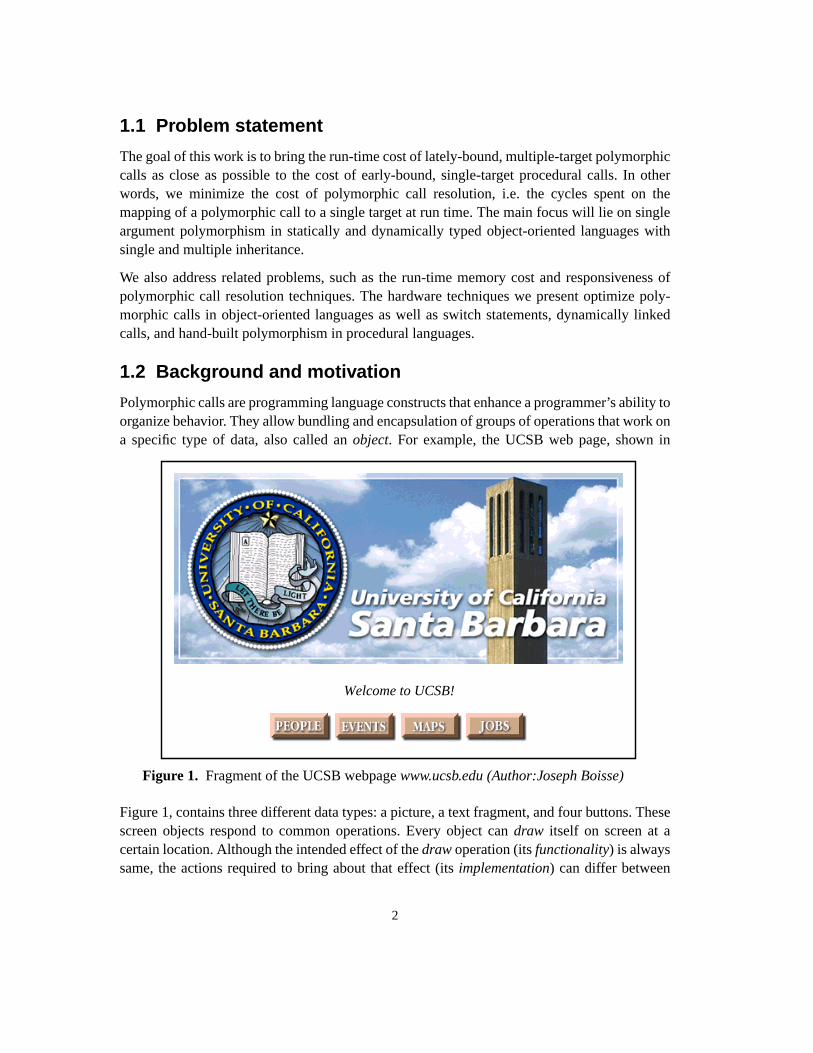
Polymorphic calls are programming language constructs that enhance a programmer’s ability toorganize behavior. They allow bundling and encapsulation of groups of operations that work ona specific type of data, also called anobject. For example, the UCSB web page, shown in

Figure 1, contains three different data types: a picture, a text fragment, and four buttons. Thesescreen objects respond to common operations. Every object candraw itself on screen at acertain location. Although the intended effect of thedraw operation (itsfunctionality) is alwayssame, the actions required to bring about that effect (itsimplementation) can differ between

Welcome to UCSB!

Figure 1. Fragment of the UCSB webpagewww.ucsb.edu (Author:Joseph Boisse)

3

object types. For example, drawing a picture on screen requires that a given two-dimensional setof pixels is placed in the screen buffer. Drawing text requires that a string is translated intopixels by looking up each character in a font map and then writing those pixels to the screenbuffer. Operations that require the execution of different subroutines depending on the type ofobject they are applied to, are calledpolymorphic.

Since each object-oriented language provides its own terminology for polymorphic operations,Table 1 shows the terms used in popular languages for easy translation. We will use the generalterms provided as headings, unless we discuss language-specific techniques.

Polymorphic calls make life easier for the user of an object library, who only has to know whatoperations mean in terms of functionality. It becomes easy to manipulate collections of objectsthat are different but share functionality such as thedraw operation.To draw a page consistingof many screen objects, a programmer merely has to calldraw on every object. It is not neces-sary to know the implementation details of each object’s type (see Figure 2).The run-timesystem intercepts the polymorphic call and redirects it to the appropriate implementation.

Language Polymorphic call ImplementationC++, Java Virtual function call Function definition

Smalltalk, SELF Message send Method

CLOS, Dylan Generic function invocation Method

Table 1. Language-specific terms for polymorphic calls

Picturedrawclick

Figure 2. Object types (classes) and polymorphic calls

Textdrawclickedit

Buttondrawclick

logoUCSB.draw();“Welcome to UCSB !”.draw();for (i = 0; i < nrOfButtons; i++) {

button[i].draw();}

Run timepolymorphiccall resolution

4

1.2.1 Inheritance

1.2.1.1 Subtyping

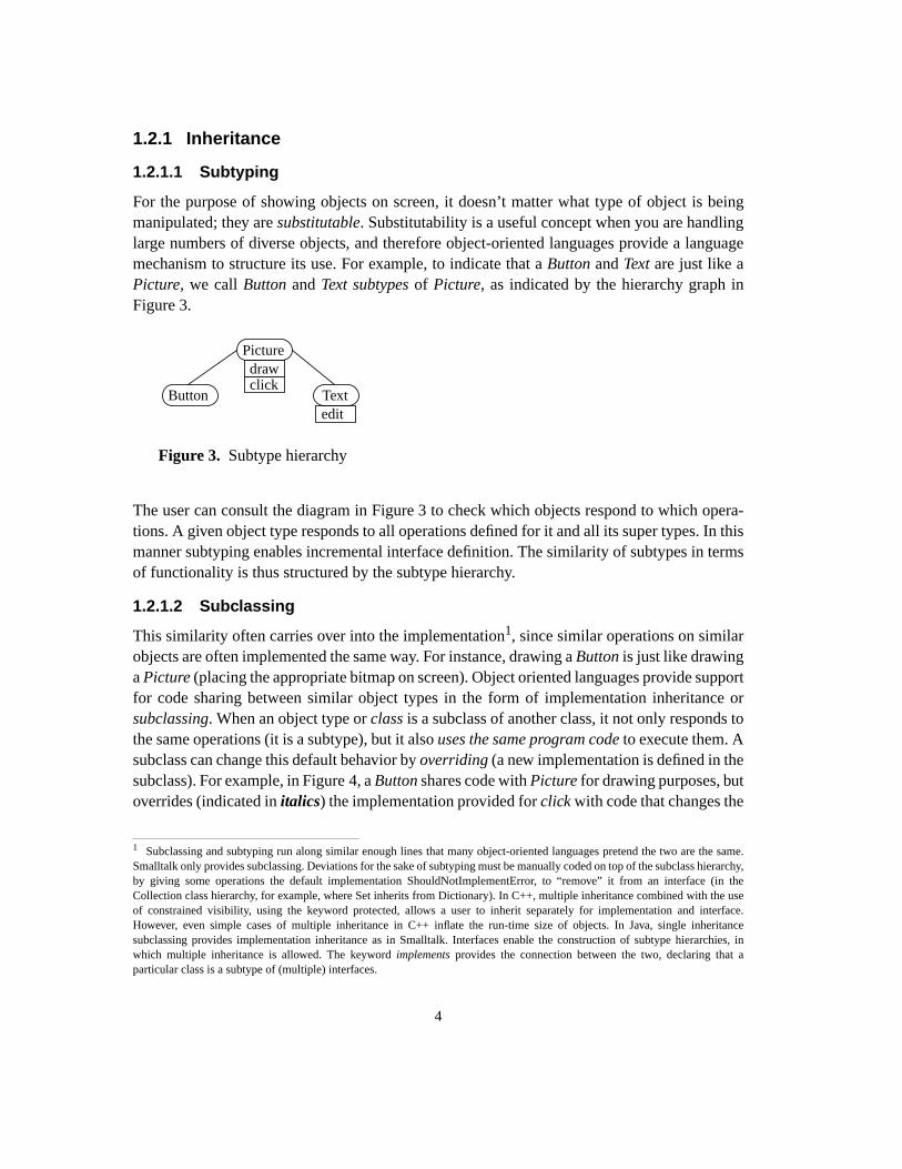
For the purpose of showing objects on screen, it doesn’t matter what type of object is beingmanipulated; they aresubstitutable. Substitutability is a useful concept when you are handlinglarge numbers of diverse objects, and therefore object-oriented languages provide a languagemechanism to structure its use. For example, to indicate that aButton andText are just like aPicture, we callButton andText subtypes of Picture, as indicated by the hierarchy graph inFigure 3.

The user can consult the diagram in Figure 3 to check which objects respond to which opera-tions. A given object type responds to all operations defined for it and all its super types. In thismanner subtyping enables incremental interface definition. The similarity of subtypes in termsof functionality is thus structured by the subtype hierarchy.

1.2.1.2 Subclassing

This similarity often carries over into the implementation1, since similar operations on similarobjects are often implemented the same way. For instance, drawing aButton is just like drawingaPicture (placing the appropriate bitmap on screen). Object oriented languages provide supportfor code sharing between similar object types in the form of implementation inheritance orsubclassing. When an object type orclass is a subclass of another class, it not only responds tothe same operations (it is a subtype), but it alsouses the same program code to execute them. Asubclass can change this default behavior byoverriding(a new implementation is defined in thesubclass). For example, in Figure 4, aButton shares code withPicture for drawing purposes, butoverrides (indicated initalics) the implementation provided forclick with code that changes the

1 Subclassing and subtyping run along similar enough lines that many object-oriented languages pretend the two are the same.Smalltalk only provides subclassing. Deviations for the sake of subtyping must be manually coded on top of the subclass hierarchy,by giving some operations the default implementation ShouldNotImplementError, to “remove” it from an interface (in theCollection class hierarchy, for example, where Set inherits from Dictionary). In C++, multiple inheritance combined with the useof constrained visibility, using the keyword protected, allows a user to inherit separately for implementation and interface.However, even simple cases of multiple inheritance in C++ inflate the run-time size of objects. In Java, single inheritancesubclassing provides implementation inheritance as in Smalltalk. Interfaces enable the construction of subtype hierarchies, inwhich multiple inheritance is allowed. The keywordimplements provides the connection between the two, declaring that aparticular class is a subtype of (multiple) interfaces.

Picturedrawclick

Figure 3. Subtype hierarchy

Textedit

Button

5

user’s perspective to a different web page.Text, on the other hand, inheritsclick but provides itsown drawing implementation and adds theedit operation to its interface and implementation.Subclassing therefore enables incremental implementation. This is useful for thebuilder of anobject library. Instead of implementing the complete interface of a class, only the differencebetween it and an appropriately chosen super class needs to be coded from scratch.

Inheritance requires polymorphic calls. Since objects are substitutable, the programmer is oftenunaware of the actual type of the objects that are manipulated. He/she relies on the system tofind and call the correct implementation for a given operation. This enhances maintainability,since objects may be designed or constructed by a third party long after the code has been deliv-ered. Only substitutability is required for the existing code to work correctly.

It is the responsibility of the language system builder to make polymorphic calls efficient. Acompiler may be able to replace some polymorphic calls by early-bound single-target calls, ifit can be proven that the call can result in only one target subroutine. However, real polymor-phism must be resolved at run time. It is our aim to reduce the run time cost of polymorphic callresolution as much as possible.

1.3 Contributions

We studied techniques, first in software, then in hardware, to reduce the cost, both in time andspace, of run-time polymorphic call resolution. In doing so, we made a number of contributionsto the field.

In software, we made the following contributions:

• Minimization of the memory overhead of dispatch tables. Table-based dispatch, a fastpolymorphic call resolution technique, was formerly restricted to statically typedprogramming languages. We increased its application domain by reducing its memoryoverhead from 95% to 36% in previous work [40]. Similar efforts by Andre and Royer [9],resulted in 43% overhead and took hours to compute. As part of the dissertation work wereduced the overhead to less than 1%, optimized the table construction algorithm to run inseconds instead of hours for large class libraries (see Section 4), and designed a variant tohandle multiple inheritance hierarchies. This makes table-based dispatch practical for twoadditional classes of programming languages: dynamically typed languages and languagesthat allow multiple inheritance.

Picturedrawclick

Textdrawedit

Buttonclick

Figure 4. Subclass hierarchy

6

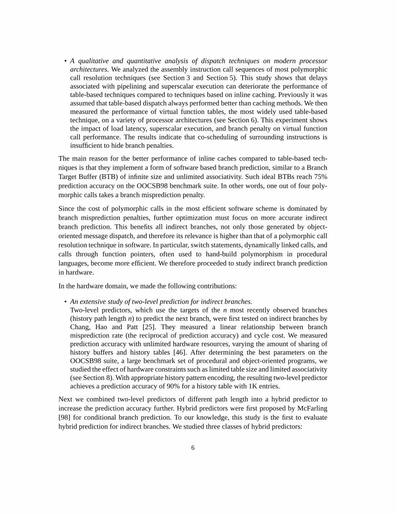
• A qualitative and quantitative analysis of dispatch techniques on modern processorarchitectures. We analyzed the assembly instruction call sequences of most polymorphiccall resolution techniques (see Section 3 and Section 5). This study shows that delaysassociated with pipelining and superscalar execution can deteriorate the performance oftable-based techniques compared to techniques based on inline caching. Previously it wasassumed that table-based dispatch always performed better than caching methods. We thenmeasured the performance of virtual function tables, the most widely used table-basedtechnique, on a variety of processor architectures (see Section 6). This experiment showsthe impact of load latency, superscalar execution, and branch penalty on virtual functioncall performance. The results indicate that co-scheduling of surrounding instructions isinsufficient to hide branch penalties.

The main reason for the better performance of inline caches compared to table-based tech-niques is that they implement a form of software based branch prediction, similar to a BranchTarget Buffer (BTB) of infinite size and unlimited associativity. Such ideal BTBs reach 75%prediction accuracy on the OOCSB98 benchmark suite. In other words, one out of four poly-morphic calls takes a branch misprediction penalty.

Since the cost of polymorphic calls in the most efficient software scheme is dominated bybranch misprediction penalties, further optimization must focus on more accurate indirectbranch prediction. This benefits all indirect branches, not only those generated by object-oriented message dispatch, and therefore its relevance is higher than that of a polymorphic callresolution technique in software. In particular, switch statements, dynamically linked calls, andcalls through function pointers, often used to hand-build polymorphism in procedurallanguages, become more efficient. We therefore proceeded to study indirect branch predictionin hardware.

In the hardware domain, we made the following contributions:

• An extensive study of two-level prediction for indirect branches.Two-level predictors, which use the targets of then most recently observed branches(history path lengthn) to predict the next branch, were first tested on indirect branches byChang, Hao and Patt [25]. They measured a linear relationship between branchmisprediction rate (the reciprocal of prediction accuracy) and cycle cost. We measuredprediction accuracy with unlimited hardware resources, varying the amount of sharing ofhistory buffers and history tables [46]. After determining the best parameters on theOOCSB98 suite, a large benchmark set of procedural and object-oriented programs, westudied the effect of hardware constraints such as limited table size and limited associativity(see Section 8). With appropriate history pattern encoding, the resulting two-level predictorachieves a prediction accuracy of 90% for a history table with 1K entries.

Next we combined two-level predictors of different path length into a hybrid predictor toincrease the prediction accuracy further. Hybrid predictors were first proposed by McFarling[98] for conditional branch prediction. To our knowledge, this study is the first to evaluatehybrid prediction for indirect branches. We studied three classes of hybrid predictors:

7

• Classifying predictors, first proposed for conditional branches by Chang, Hao and Patt [23],assign a class to each branch according to compile-time or profile-based criteria. Wededicate a separate two-level predictor to each class, with a separately tuned path length(see Section 9.2). The best of the tested predictors achieves 91% prediction accuracy for 1Ktable entries, but requires a change in the instruction set architecture.

• Dual-path hybrid predictors, use two two-level predictors of different path length, updateboth for each branch and use the prediction with the highest 2-bit confidence counter (seeSection 9.3). This dynamically updated counter keeps track of the number of successesamong the last 3 predictions of a table entry. After tuning, the best predictor achieves 91%prediction accuracy for 1K total table entries.

• Cascaded predictors, a new prediction architecture (see Section 9.4), use several stages oftwo-level predictors of different path length, and give precedence to the longest path lengthprediction available. In addition, pattern filtering reduces the number of table entriesrequired to reach a particular prediction accuracy. When updating, a cascaded predictorprevents insertion of a pattern into the longer path length component if the shorter pathlength prediction is correct. The best combination with a BTB as first stage resulted in 92%prediction accuracy for 1K total table entries. A cascaded predictor reduces the cost of atwo-level predictor by a factor four, for similar prediction accuracy. At 6K entries, a 3-stagecascaded predictor with tuned path lengths reaches 95% prediction accuracy, higher thanthe 94% accuracy achieved by a hypothetical two-level predictor with an unlimited, fullyassociative predictor table.

Combined, the software contributions minimize the cost of a polymorphic call innumber ofinstructions, while the hardware advances minimize the cost of these instructions innumber ofprocessor cycles.At affordable off-chip memory costs and on-chip transistor budgets, well-tuned software and hardware support can bring the run-time overhead of polymorphic call reso-lution down to an insignificant fraction of total run time, as measured on various industry-sizebenchmarks.

8

1.4 Overview

This dissertation is organized in sections that correspond to the different fields the work touchesupon. Section 2 describes variations of the polymorphic call construct and states the problemwe address in this work. Section 3 presents the major software techniques for efficient polymor-phic call resolution and compares their memory overhead and program environmentconstraints. Section 4 presents and measures a new algorithm for memory overhead reductionof dispatch tables.

The next two sections evaluate the run-time performance of software techniques by qualitativeand quantitative analysis of the software-hardware interface. In Section 5 we establishesbounds on the performance of table-based techniques on different processor generations andestimate average cycle overhead of dynamic techniques. In Section 6 we measure the overheadof virtual function table dispatch by cycle-level simulation, and study the effect on call resolu-tion overhead of processor characteristics like instruction issue, load latency, and indirectbranch prediction.

The remaining sections deal with hardware techniques. In Section 7 we discuss the hardwarecontext, present benchmark programs and our method of investigation. In Section 8 we measureand reduce history pattern interference misses, capacity and conflict misses of basic path-basedpredictors. Section 9 studies three classes of path-based hybrid predictors, and presents thecascaded predictor, a new architecture which reduces the cost of indirect branch predictor tablesby a factor four. Section 10 discusses related work not mentioned in the survey chapters.Section 12 concludes. Section 11 discusses open problems and future work.

9

2 Polymorphic calls“Polymorphism: In biology, the coexistence oftwo or more genetically distinct forms of anorganism within the same interbreeding popula-tion, where the frequency of the rarest type is notmaintained by mutation alone. Human eye colouris an example of a readily observable polymor-phism, but there are many invisible polymor-phisms detectable only by special techniques,such as DNA analysis”,

The Cambridge Encyclopedia[15]

In this section we discuss the polymorphic call construct as it appears in different programminglanguages.

2.1 Basic construct

Polymorphism is a powerful programming construct because it allows a programmer to invokean operation on a piece of data by specifying the intended effect, without having to worry aboutthe implementation details on different kinds of datatypes. Using the webpage example intro-duced in Section 1, non-polymorphic code to draw the page could look as follows:

logoUCSB.drawPicture();“Welcome to UCSB !”.drawText();for (i = 0; i < nrOfButtons; i++) {

button[i].drawButton();}

The programmer has to specify the right drawing operation for each screen object. Polymorphiccode looks like this:

logoUCSB.draw();“Welcome to UCSB !”.draw();for (i = 0; i < nrOfButtons; i++) {

button[i].draw();}

or even simpler:

for (i = 0; i < nrOfScreenObjects; i++) {screenObject[i].draw();

}

In polymorphic code, the programmer is free of the concern to match the right drawing opera-tion to each screen object. The run-time system distinguishes different screen objects andinvokes the right implementation of thedraw operation. This allows rapid prototyping, and

10

code that is easier to maintain, since the introduction of a new screen object, for example, aframed picture, does not force rewriting of alldrawPicture invocations. A new implementationof draw must be provided, and from then on, all program code that manipulates pictures throughthe public interface of thePicture class is equally capable of dealing with framed pictures.

2.2 Polymorphic calls in procedural languages

Procedural languages give no support for polymorphism. However, since it is a useful abstrac-tion tool, hand-crafted polymorphic calls are often found in procedural programs. The keymechanism is to remove the type-specific procedure invocations from the call point, replacingthem by a single procedure invocation, and resolving the polymorphism in the called procedure.For example, a polymorphicdraw procedure could be implemented as follows:

draw (screenObject o) {switch (o.type) {

case picture: drawPicture(o); break;case text: drawText(o); break;case button: drawButton(o); break;default: error(“draw undefined for object”);

}

Though this construction removes implementation concerns from the calling point, theprogrammer must hand-craft polymorphism resolution procedures for every polymorphic oper-ation. Implementation of call resolution on the run-time system level removes this repetitiveburden from the programmer. It also allows more radical optimization because run-time imple-mentation requires only a one time implementation effort.

Hand-crafted polymorphism has its flaws also from a maintenance perspective. Relationshipsbetween types are encoded ad-hoc in the polymorphic call procedures. When a new data type isintroduced, all polymorphic procedures that handle the type must be augmented, and this codechange is dispersed over many different places in the program. In object-oriented languages, amore systematic approach allows the programmer to define all the new code in one place, andtake advantage of implementation inheritance to minimize the extra implementation effort.

2.3 Object-oriented message dispatch

Object-oriented languages allow the definition of a datatype and its associated operations in oneplace, typically called a class or a prototype object. In our example, the programmer provideseach screen object with adraw implementation, and the system will ensure that the right imple-mentation is called for each type. In object-oriented languages, like Smalltalk, polymorphiccalls are known asmessage sends and polymorphic call resolution is calledmessage dispatch.The different class-specific implementations of a message are calledmethods. Implementationinheritance allows default methods to be defined for sets of classes. For instance, thedraw

11

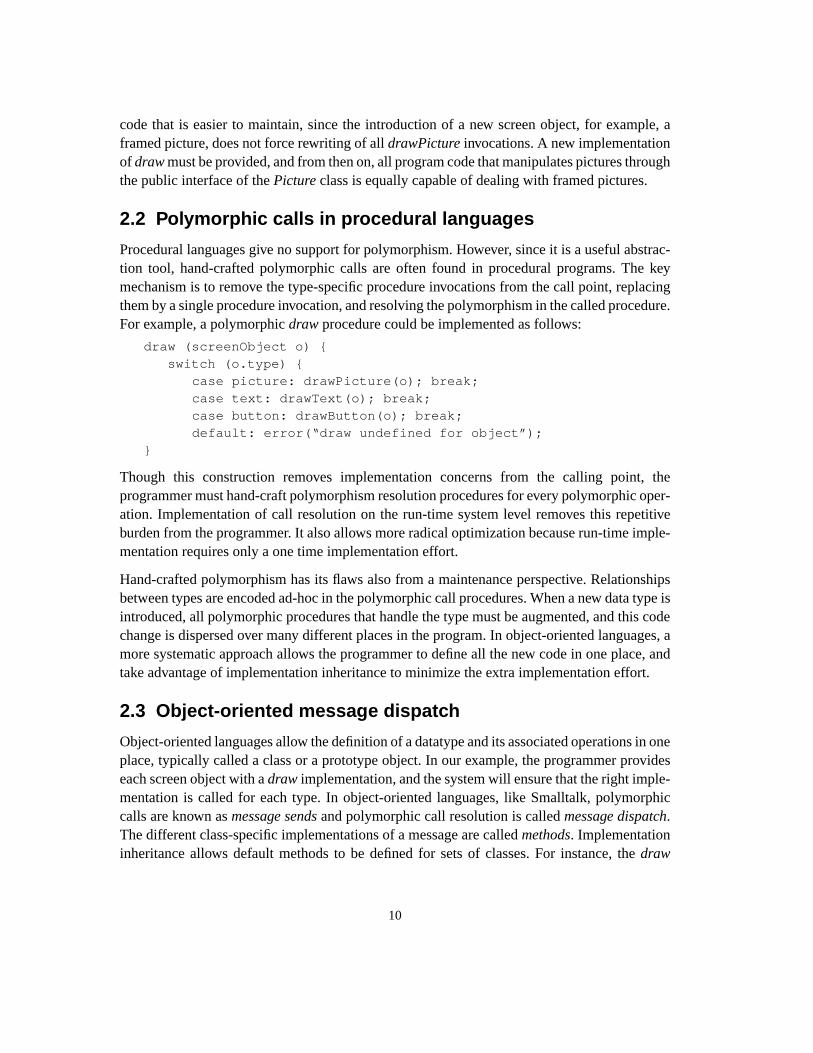
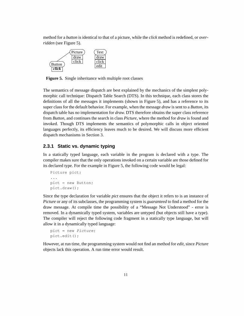
method for abutton is identical to that of a picture, while theclick method is redefined, orover-ridden(see Figure 5).

The semantics of message dispatch are best explained by the mechanics of the simplest poly-morphic call technique: Dispatch Table Search (DTS). In this technique, each class stores thedefinitions of all the messages it implements (shown in Figure 5), and has a reference to itssuper class for the default behavior. For example, when the messagedraw is sent to aButton, itsdispatch table has no implementation fordraw. DTS therefore obtains the super class referencefrom Button, and continues the search in classPicture, where the method fordraw is found andinvoked. Though DTS implements the semantics of polymorphic calls in object orientedlanguages perfectly, its efficiency leaves much to be desired. We will discuss more efficientdispatch mechanisms in Section 3.

2.3.1 Static vs. dynamic typing

In a statically typed language, each variable in the program is declared with a type. Thecompiler makes sure that the only operations invoked on a certain variable are those defined forits declared type. For the example in Figure 5, the following code would be legal:

Picture pict;...pict = new Button;pict.draw();

Since the type declaration for variablepict ensures that the object it refers to is an instance ofPicture or any of its subclasses, the programming system isguaranteed to find a method for thedraw message. At compile time the possibility of a “Message Not Understood” - error isremoved. In a dynamically typed system, variables are untyped (but objects still have a type).The compiler will reject the following code fragment in a statically type language, but willallow it in a dynamically typed language:

pict = new Picture ;pict.edit();

However, at run time, the programming system would not find an method foredit, sincePictureobjects lack this operation. A run time error would result.

Figure 5. Single inheritance with multiple root classes

Picturedrawclick

Textdraw

editButtonclick

click

12

Statically typed languages make it easier for the programming system to implement messagedispatch efficiently, since the number of different messages that can be sent to a variable islimited and a method always exists. In a dynamically typed language, any message can be sentto any object, so the number of possibilities is much larger, and the system must be able tohandle the case where no method can be found. Dynamically typed languages offer greater flex-ibility, by not requiring that all possible receivers of a given message share a common ancestorthat defines the message. For example, the following code is incorrect in a statically typedlanguage, but both allowed and error free in a dynamically typed language (assuming the inher-itance hierarchy in Figure 5):

if (test) {obj = new Text;

} else {obj = new Button;

}obj.draw();

Although bothText andButton understand the messagedraw, static typing would not allow theassignment of instances of these classes to the same variable, because they do not share acommon superclass in whichdraw is defined1.

2.3.2 Single vs. multiple inheritance

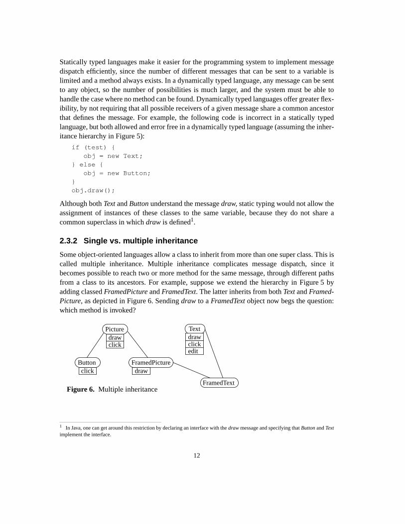
Some object-oriented languages allow a class to inherit from more than one super class. This iscalled multiple inheritance. Multiple inheritance complicates message dispatch, since itbecomes possible to reach two or more method for the same message, through different pathsfrom a class to its ancestors. For example, suppose we extend the hierarchy in Figure 5 byadding classedFramedPicture andFramedText. The latter inherits from bothText andFramed-Picture, as depicted in Figure 6. Sendingdraw to aFramedText object now begs the question:which method is invoked?

1 In Java, one can get around this restriction by declaring an interface with thedraw message and specifying thatButton andTextimplement the interface.

Figure 6. Multiple inheritance

Picturedrawclick

Buttonclick

FramedPicturedraw

Text

FramedText

drawclickedit

13

Different programming languages give different answers: in CLOS [107], the programmer liststhe super classes of a class in a certain order, and this tells the programming system which classtakes priority. In C++, this kind of ambiguity causes a compile-time error. The programmer canspecify which path takes precedence, for example by callingText::draw. This practice partiallybreaks down the abstraction mechanism provided by polymorphism, since the programmer nowhas to limit the choice of method at the calling point. From an implementation perspective thesemantics do not matter much, as long as thedraw call resolves to a unique method.

Multiple inheritance complicates efficient polymorphic call resolution, since a class no longerextends an existing set of operations with a few extra messages, but merges two or more sets.Compile-time construction of compact dispatch tables becomes harder in that case, as discussedin Section 4.

2.3.3 Single vs. multiple dispatch

In most object-oriented languages, the type of one privileged argument, called thereceiver,determines the method to invoke for a polymorphic call. Languages like CECIL [18] and CLOS[83] allow the types of other arguments to further refine the choice of method. This can beuseful, for example to allow the draw operation to display graphical objects on different media,like a screen or a postscript printer. Both the type of the object to be drawn, and the medium onwhich it is drawn, determine the procedure to be invoked:

for (i = 0; i < nrOfObjects; i++) {object[i].draw(medium);

}

The standard solution to multiple dispatch in languages that only provide single argumentdispatch is a technique calleddouble dispatch [75]. The programmer writes each draw opera-tion in a graphical object class as follows (for example in thePicture andText classes, withmediaScreen andPostscriptPrinter, and whereTHIS is the object for which the draw operationwas invoked):

class Picturedraw (medium)

medium.drawPicture(THIS);

class Textdraw (medium)

medium.drawText(THIS);

14

class ScreendrawPicture (picture)

// code for drawing a picture on a screen

drawText (text)// code for drawing text on a screen

class PostscriptPrinterdrawPicture (picture)

// code for drawing a picture on a postscript printer

drawText (text)// code for drawing text on a postscript printer

Dispatch over two arguments is emulated by two successive single-argument dispatches. Thistechnique has several disadvantages. First, the programmer is responsible for the maintenanceof double dispatch code, similar to the hand-crafted polymorphic call resolution procedures thatimplement single argument dispatch in procedural languages. Second, double dispatch isslower than multiple dispatch. Multiple dispatch executes parameter passing code only once,and can employ more advanced call sequence optimization. In practice, programmers do notoften employ multiple dispatch, even in languages that support it. Single-argument dispatchremains the common case (see [44]). We will not explore multiple dispatch techniques in depth(however, see section 10.1.3 for an analysis).

2.3.4 Predicate dispatch

Ernst, Kaplan and Chambers present a unified model of dispatch [55], based on predicateexpressions that serve as guards to multiple implementations of the same generic function.Since predicate expressions can be arbitrary side-effect free expressions, this model captures allvariants defined above, as well as ML-style pattern matching, predicate classes, and classifiers.From a language design perspective, such a powerful dispatch mechanism is ideal, because itallows the programmer to use the style best fit to model a specific problem, or even to constructa personal style. From an implementation perspective, predicate dispatch presents a big chal-lenge. We believe that a combination of compile-time and run-time techniques will be neces-sary to reduce its cost and make it attractive to performance-conscious practitioners. Single-argument message dispatch is likely to remain the most frequent operation in most programs,and a general dispatch mechanism for predicate dispatch must therefore incorporate an efficienttechnique for this common case. Chambers and Chen [20] present efficient implementation ofmultiple and predicate dispatch, which combines efficient techniques for single dispatching,multiple dispatching, and predicate dispatching. All these cases are implemented as a series ofsingle dispatches where each single dispatch is implemented with the technique appropriate forthe type of call. For example, if the number of targets is large, a table based implementation ischosen instead of a linear search.

15

3 Software techniques for efficient polymorphic calls“Swiss Army Knife. A tool that makes thecommon task easy, while providing all the neces-sary tools for the most general task.”

Jennifer West [132]

In this section, we describe the major techniques in current use for the optimization of polymor-phic calls. We present the techniques and discuss run-time aspects like estimated memory costand responsiveness. Detailed estimates of run-time call cost are delayed until Section 5, wherewe bring hardware into the picture.

3.1 Basic message dispatch in object-oriented languages

In object-oriented languages, polymorphic call resolution is calledmessage dispatch. Messagedispatch is a function that takes the message name (selector) and the class of its first argument(receiver), and matches this pair to the correct implementation, also calledmethod. If methodlookup speed was unimportant, dispatch could be performed by searching class-specificdispatch tables. When an object receives a message, the object’s class is searched for the corre-sponding method, and if no method is found the lookup proceeds in the super class(es). Sinceit searches dispatch tables for methods, this technique is called Dispatch Table Search (DTS).The right-hand side of Figure 7 shows the dispatch tables of the class hierarchy on the left. Eachentry in a dispatch table contains the method name and a number representing its address. As inall other figures, capital letters (A, B, C) denote classes and lowercase letters denote methods.

Since the memory requirements of DTS are minimal (i.e., proportional to the number ofmethods in the system), DTS is often used as a backup strategy which is invoked when fastermethods fail. Typically, DTS implementations employ hashing to speed up the table search.

All of the techniques discussed in the remainder of this chapter improve upon the speed of DTSby precomputing or caching lookup results. The dispatch techniques studied here fall into twocategories.Static techniques precompute all data structures at compile or link time and do notchange those data structures at run-time. Thus, static techniques only use information that can

a a0AA

B acf C e

E bdD f

Figure 7. Class hierarchy with corresponding dispatch tables

c1B f

2a3

e4C

f5D

g6

b7E d

8g

16

be statically derived from the program’s source text.Dynamic techniques may precomputesome information at compile or link time, but they dynamically update data structures at run-time, i.e., during program execution. Thus, dynamic techniques can exploit run-time informa-tion as well as static information. Table 2 lists the techniques we studied.

3.1.1 Influence of dynamic typing

In dynamically-typed languages, a program may try to invoke an operation on some object forwhich the operation is undefined (“message not understood” error). Therefore, each messagedispatch usually needs to include some form of run-time check to guarantee that such errors areproperly caught and reported to the user. Most techniques that support static typing can beextended to handle dynamic typing as well. Our study shows the additional dispatch cost ofdynamic typing for all dispatch mechanisms that can support it.

3.1.2 Influence of multiple inheritance

A system using multiple inheritance (MI) introduces an additional difficulty if compiled codeuses hard-coded offsets when addressing instance variables. For example, assume that classCinherits directly from classesA andB (Figure 8). In order to reuse compiled code of classA,instances ofC would have to start with the instance variables ofA (i.e.,A’s memory layout mustbe a prefix ofC’s layout). But the compiled code in classB requires a conflicting memory layout(B’s instance variables must come first), and so it seems that compiled code cannot be reused ifit directly addresses instance variables of an object.

Hard-coded offsets can be retained, in a statically typed setting, if the receiver object’s addressis adjusted just before aB method is executed, so that it points to theB sub-object withinC [87,53] (thecurrent type isB). Within the called method, thecurrent type’s instance variable offsetsand the position of its virtual function table are compile time constants. If the same method iscalled from different sub-objects, different pointer adjustments are required. Therefore each

Acronym Full Name Section

stat

icte

chni

ques

DTS Dispatch Table Search (used for illustration only) 3.1

STI Selector Table Indexing (used for illustration only) 3.3.1

VTBL Virtual Function Tables, single inheritance 3.3.2

VTBL-MI Virtual Function Tables, full version 3.3.2

SC Selector Coloring 3.3.3

RD Row Displacement 3.3.4

CT Compact Tables 3.3.5

dyna

m.

tech

n. LC Lookup Caching 3.2.1

IC Inline Caching 3.2.2

PIC Polymorphic Inline Caching 3.2.3

Table 2. Overview of dispatch methods

17

sub-object points to its own table, in which an extra entry for each function stores the size of theadjustment. However, in a dynamically-typed setting, the structure of the object is unknown atcompile time. Therefore we assume that techniques capable of dealing with dynamic typing usethe following approach to access instance variables in the multiple inheritance case:

• always use accessor messages, except to access instance variables from self1.

• use hard-coded offsets for self instance variables, and maintain a different compiled versionfor every method of a class that accesses them, whenever it is combined with a different co-parent.

Under this constraint, all techniques studied here (except VTBL for older processors) shownear-identical performance for single and multiple inheritance. We discuss both a single- and amultiple inheritance version for VTBL. The space overhead caused by multiple inheritance istreated, for all techniques, in Section 3.4.2.

Each description of a dispatch technique includes pseudo-code illustrating the run-timedispatch. Since our analysis separates out the influence of dynamic typing and multiple inher-itance/hardwired instance variable offsets, two typographical conventions mark code used tosupport one of these functions.Italic code supports multiple inheritance, andbold codesupports dynamic typing. Appendix A collects the assembly call sequences and instructionscheduling.

3.2 Dynamic techniques

Dynamic techniques speed up message lookup by using various forms of caching at run-time.Therefore, they depend on locality properties of object-oriented programs: caching will speedup programs if the cached information is used often before it is evicted from the cache. Thissection discusses two kinds of caching: global caching (one large cache per system) and inlinecaching (one one-entry cache per call site).

1 This is done in SELF [16]. Indirect instance variable access is used in Eiffel and Sather [102].

Figure 8. Memory layout of objects in the case of multiple inheritance.

paa1A B

C

...

pbb1...

pca1...c1...b1...

adjusted pb

A

C

B

The offset of instance variableb1 is different in instances ofB versusinstances ofC.

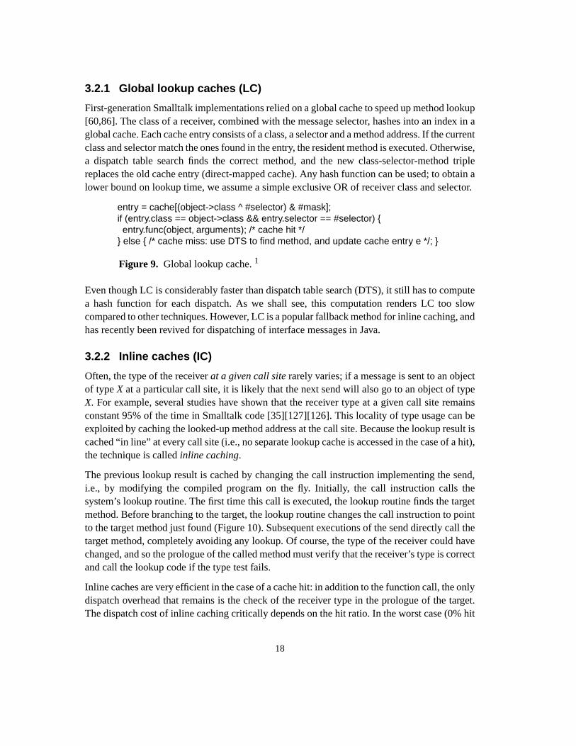
18

3.2.1 Global lookup caches (LC)

First-generation Smalltalk implementations relied on a global cache to speed up method lookup[60,86]. The class of a receiver, combined with the message selector, hashes into an index in aglobal cache. Each cache entry consists of a class, a selector and a method address. If the currentclass and selector match the ones found in the entry, the resident method is executed. Otherwise,a dispatch table search finds the correct method, and the new class-selector-method triplereplaces the old cache entry (direct-mapped cache). Any hash function can be used; to obtain alower bound on lookup time, we assume a simple exclusive OR of receiver class and selector.

Even though LC is considerably faster than dispatch table search (DTS), it still has to computea hash function for each dispatch. As we shall see, this computation renders LC too slowcompared to other techniques. However, LC is a popular fallback method for inline caching, andhas recently been revived for dispatching of interface messages in Java.

3.2.2 Inline caches (IC)

Often, the type of the receiverat a given call site rarely varies; if a message is sent to an objectof typeX at a particular call site, it is likely that the next send will also go to an object of typeX. For example, several studies have shown that the receiver type at a given call site remainsconstant 95% of the time in Smalltalk code [35][127][126]. This locality of type usage can beexploited by caching the looked-up method address at the call site. Because the lookup result iscached “in line” at every call site (i.e., no separate lookup cache is accessed in the case of a hit),the technique is calledinline caching.

The previous lookup result is cached by changing the call instruction implementing the send,i.e., by modifying the compiled program on the fly. Initially, the call instruction calls thesystem’s lookup routine. The first time this call is executed, the lookup routine finds the targetmethod. Before branching to the target, the lookup routine changes the call instruction to pointto the target method just found (Figure 10). Subsequent executions of the send directly call thetarget method, completely avoiding any lookup. Of course, the type of the receiver could havechanged, and so the prologue of the called method must verify that the receiver’s type is correctand call the lookup code if the type test fails.

Inline caches are very efficient in the case of a cache hit: in addition to the function call, the onlydispatch overhead that remains is the check of the receiver type in the prologue of the target.The dispatch cost of inline caching critically depends on the hit ratio. In the worst case (0% hit

entry = cache[(object->class ^ #selector) & #mask];if (entry.class == object->class && entry.selector == #selector) {entry.func(object, arguments); /* cache hit */

} else { /* cache miss: use DTS to find method, and update cache entry e */; }

Figure 9. Global lookup cache.1

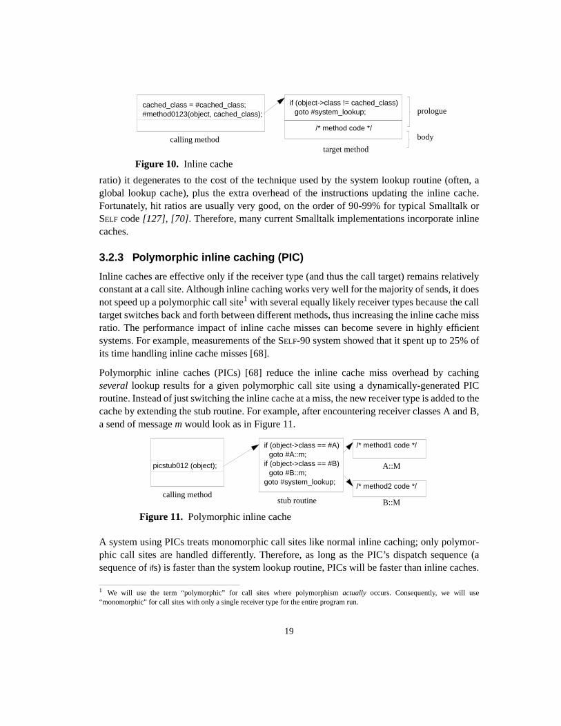
19

ratio) it degenerates to the cost of the technique used by the system lookup routine (often, aglobal lookup cache), plus the extra overhead of the instructions updating the inline cache.Fortunately, hit ratios are usually very good, on the order of 90-99% for typical Smalltalk orSELF code[127], [70] . Therefore, many current Smalltalk implementations incorporate inlinecaches.

3.2.3 Polymorphic inline caching (PIC)

Inline caches are effective only if the receiver type (and thus the call target) remains relativelyconstant at a call site. Although inline caching works very well for the majority of sends, it doesnot speed up a polymorphic call site1 with several equally likely receiver types because the calltarget switches back and forth between different methods, thus increasing the inline cache missratio. The performance impact of inline cache misses can become severe in highly efficientsystems. For example, measurements of the SELF-90 system showed that it spent up to 25% ofits time handling inline cache misses [68].

Polymorphic inline caches (PICs) [68] reduce the inline cache miss overhead by cachingseveral lookup results for a given polymorphic call site using a dynamically-generated PICroutine. Instead of just switching the inline cache at a miss, the new receiver type is added to thecache by extending the stub routine. For example, after encountering receiver classes A and B,a send of messagem would look as in Figure 11.

A system using PICs treats monomorphic call sites like normal inline caching; only polymor-phic call sites are handled differently. Therefore, as long as the PIC’s dispatch sequence (asequence ofifs) is faster than the system lookup routine, PICs will be faster than inline caches.

1 We will use the term “polymorphic” for call sites where polymorphismactually occurs. Consequently, we will use“monomorphic” for call sites with only a single receiver type for the entire program run.

cached_class = #cached_class;#method0123(object, cached_class);

/* method code */

Figure 10. Inline cache

calling method body

prologue

target method

if (object->class != cached_class)goto #system_lookup;

if (object->class == #A)goto #A::m;

if (object->class == #B)goto #B::m;

goto #system_lookup;

Figure 11. Polymorphic inline cache

picstub012 (object);

calling methodstub routine

A::M

/* method1 code */

B::M

/* method2 code */

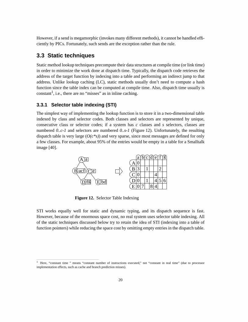
20

However, if a send is megamorphic (invokes many different methods), it cannot be handled effi-ciently by PICs. Fortunately, such sends are the exception rather than the rule.

3.3 Static techniques

Static method lookup techniques precompute their data structures at compile time (or link time)in order to minimize the work done at dispatch time. Typically, the dispatch code retrieves theaddress of the target function by indexing into a table and performing an indirect jump to thataddress. Unlike lookup caching (LC), static methods usually don’t need to compute a hashfunction since the table index can be computed at compile time. Also, dispatch time usually isconstant1, i.e., there are no “misses” as in inline caching.

3.3.1 Selector table indexing (STI)

The simplest way of implementing the lookup function is to store it in a two-dimensional tableindexed by class and selector codes. Both classes and selectors are represented by unique,consecutive class or selector codes; if a system hasc classes ands selectors, classes arenumbered0..c-1 and selectors are numbered0..s-1 (Figure 12). Unfortunately, the resultingdispatch table is very large (O(c*s)) and very sparse, since most messages are defined for onlya few classes. For example, about 95% of the entries would be empty in a table for a Smalltalkimage [40].

STI works equally well for static and dynamic typing, and its dispatch sequence is fast.However, because of the enormous space cost, no real system uses selector table indexing. Allof the static techniques discussed below try to retain the idea of STI (indexing into a table offunction pointers) while reducing the space cost by omitting empty entries in the dispatch table.

1 Here, “constant time ” means “constant number of instructions executed,” not “constant in real time” (due to processorimplementation effects, such as cache and branch prediction misses).

Figure 12. Selector Table Indexing

aA

B acf C e

E bdD fg

Aa0

b c d e f g

B 3 1 2C 0 4D 0 1 4 5 6E 0 7 8 4

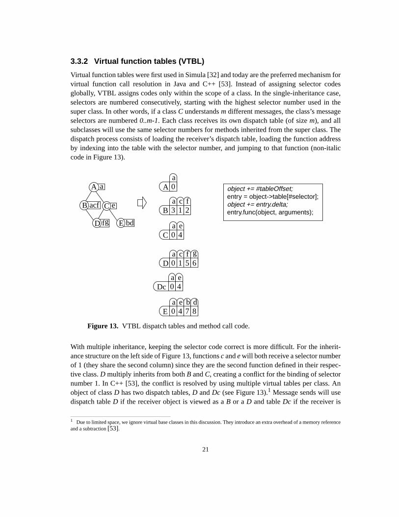
21

3.3.2 Virtual function tables (VTBL)

Virtual function tables were first used in Simula [32] and today are the preferred mechanism forvirtual function call resolution in Java and C++ [53]. Instead of assigning selector codesglobally, VTBL assigns codes only within the scope of a class. In the single-inheritance case,selectors are numbered consecutively, starting with the highest selector number used in thesuper class. In other words, if a classC understandsm different messages, the class’s messageselectors are numbered0..m-1. Each class receives its own dispatch table (of sizem), and allsubclasses will use the same selector numbers for methods inherited from the super class. Thedispatch process consists of loading the receiver’s dispatch table, loading the function addressby indexing into the table with the selector number, and jumping to that function (non-italiccode in Figure 13).

With multiple inheritance, keeping the selector code correct is more difficult. For the inherit-ance structure on the left side of Figure 13, functionsc ande will both receive a selector numberof 1 (they share the second column) since they are the second function defined in their respec-tive class.D multiply inherits from bothB andC, creating a conflict for the binding of selectornumber 1. In C++ [53], the conflict is resolved by using multiple virtual tables per class. Anobject of classD has two dispatch tables, D andDc (see Figure 13).1 Message sends will usedispatch tableD if the receiver object is viewed as aB or aD and tableDc if the receiver is

1 Due to limited space, we ignore virtual base classes in this discussion. They introduce an extra overhead of a memory referenceand a subtraction[53].

Figure 13. VTBL dispatch tables and method call code.

aA

B acf C e

E bdD fg

object += #tableOffset;entry = object->table[#selector];object += entry.delta;entry.func(object, arguments);

Aa0

Ba3

Ca0

c1

f2

e4

Da0

c1

f5

g6

Dca0

e4

Ea0

e4

b7

d8

22

viewed as a C. As explained in Section 3.1.2, the dispatch code will also adjust the receiveraddress before calling a method defined inC (theitalic code in Figure 13)

VTBL depends on static typing: without knowing the set of messages sent to an object, thesystem cannot reuse message numbers in unrelated classes (such as using 0 for the first methoddefined in a top-level class). Thus, with dynamic typing, VTBL dispatch tables would degen-erate to STI tables since any arbitrary message could be sent to an object, forcing selectornumbers to be globally unique.

3.3.3 Selector coloring (SC)

Selector coloring, first proposed by Dixon et al. [38], and applied to Smalltalk by Andre andRoyer [9], is a compromise between VTBL and STI. SC is similar to STI, but instead of usingthe selector to index into the table, SC uses the selector’scolor. The color is a number that isunique within every class where the selector is known, and two selectors can share a color ifthey never co-occur in a class. SC allows more compaction than STI, where selectors nevershare colors, but less compaction than VTBL, where a selector need not have a single globalnumber (i.e., where the selectorm can have two different numbers in unrelated classes).

Optimally assigning colors to selectors is equivalent to the graph coloring problem1 which isNP-complete. However, efficient approximation algorithms can often approach or even reachthe minimal number of colors (which is at least equal to the maximum number of messagesunderstood by any particular class). The resulting global dispatch table is much smaller than in

1 The selectors are the nodes of the graph, and two nodes are connected by an arc if the two selectors co-occur in any class.

fc

Figure 14. Selector coloring tables, method call code, and method prologue

entry = object->table[#color];entry.func(object, #selector , args)

/* method prologue */if (S != #mySelector)

error(“Message Not Understood”);

Aa0

b c d e f g

B 3 1 2C 0 4D 0 1 4 5 6E 0 7 8 4

Aa0

b d e g

B 3 1 2C 0 4D 0 1 5 4 6E 0 7 8 4

(dynamic typing inbold )

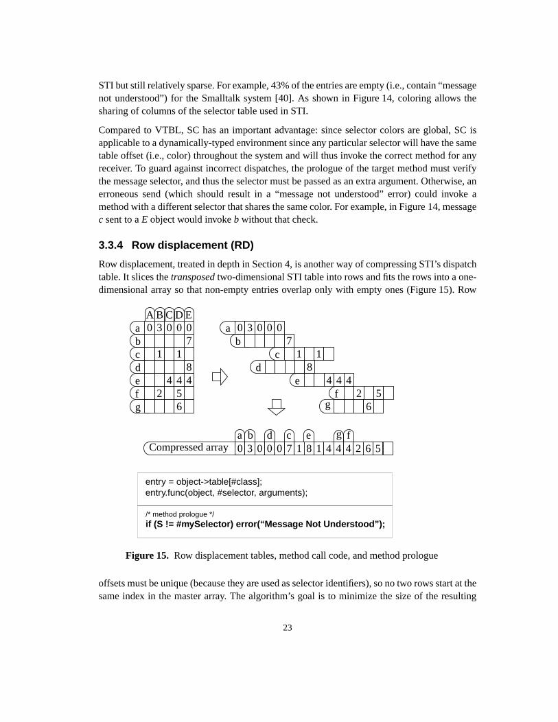
23

STI but still relatively sparse. For example, 43% of the entries are empty (i.e., contain “messagenot understood”) for the Smalltalk system [40]. As shown in Figure 14, coloring allows thesharing of columns of the selector table used in STI.

Compared to VTBL, SC has an important advantage: since selector colors are global, SC isapplicable to a dynamically-typed environment since any particular selector will have the sametable offset (i.e., color) throughout the system and will thus invoke the correct method for anyreceiver. To guard against incorrect dispatches, the prologue of the target method must verifythe message selector, and thus the selector must be passed as an extra argument. Otherwise, anerroneous send (which should result in a “message not understood” error) could invoke amethod with a different selector that shares the same color. For example, in Figure 14, messagec sent to aE object would invoke b without that check.

3.3.4 Row displacement (RD)

Row displacement, treated in depth in Section 4, is another way of compressing STI’s dispatchtable. It slices thetransposed two-dimensional STI table into rows and fits the rows into a one-dimensional array so that non-empty entries overlap only with empty ones (Figure 15). Row

offsets must be unique (because they are used as selector identifiers), so no two rows start at thesame index in the master array. The algorithm’s goal is to minimize the size of the resulting

fca b d e

Figure 15. Row displacement tables, method call code, and method prologue

/* method prologue */if (S != #mySelector) error(“Message Not Understood”);

entry = object->table[#class];entry.func(object, #selector, arguments);

a 0 3 0 0 0b 7c 1 1d 8e 4 4 4f 2 5g 6

a 0 3 0 0 0b 7

c 1 1d 8

e 4 4 4f 2 5

g 6

A B C D E

Compressed array0 3 0 0 0 7 1 8 1 4 4 2 6 5g4

24

master array by minimizing the number of empty entries; this problem is similar to parse tableminimization for table-driven parsers [34]. We first studied row displacement of the non-trans-posed STI table, a technique which generates a slice per class, using a selector numberingscheme that leaves only 33% of the entries empty for the Smalltalk image[39]. If the table issliced according to selectors (as shown in Figure 15), the number of empty entries is reduced to0.4% with an appropriate class numbering scheme [43]. We will discuss in depth why selector-based tables (row displacement of thetransposed STI table) lead to better compression inSection 4. Like SC, RD is applicable to dynamically-typed languages. As in SC, a check isneeded in the method prologue, this time to ensure that the method actually is part of thedispatch table of the receiver’s class. Therefore, the selector number is passed as an argumentto the method.

3.3.5 Compact selector-indexed dispatch tables (CT)

The third table compaction method, proposed by Vitek and Horspool [128], unlike the twoprevious methods, generates selector-specific dispatch code sequences. The technique separatesselectors into two categories.Standard selectors have one main definition and are only over-ridden in the subclasses (e.g.,a andb in Figure 16.Conflict selectors have multiple definitionsin unrelated portions of the class hierarchy (e.g.,e in Figure 16 which is defined in the unrelatedclassesC andD). CT uses two dispatch tables, a main table for standard selectors and a conflicttable for conflict selectors.

ace

ac3B 1

0A

0C5D 2

0E

6

a b c

Figure 16. Construction of Compact Tables

A a

B C be

E bD 7

BA

CDE

4

9

4

e

(a)

c

3B0A

0C5D0E

6

a b

1

2

7

(b)

A

A

c

3B

0EC5D

a b1

2

BCD

E4

9

e

(c) 6 7

5 23 10 4 9

CE

A

B D E

BC

A

D

(d)6 7

(a)main dispatch table and conflict tables fore(b)main dispatch table withc andb aliased(c)conflict tables for (A, B) and (C, E) shared, main dispatchtables for (A, C, E) overloaded(d) dispatch table fitted on a single master array, main dispatchtable for (A, C, E) trimmed

25

Standard selectors can be numbered in a simple top-down traversal of the class hierarchy; twoselectors can share a number as long as they are defined in different branches of the hierarchy.Such sharing is impossible for conflict selectors, and so the conflict table remains sparse. Butthe allocation of both tables can be further optimized. First, tables with identical entries (suchas the conflict tables forC andE) can be shared. Second, tables meeting a certain similaritycriterion—a parameter to the algorithm—can beoverloaded; divergent entries refer to a codestub which selects the appropriate method based on the type (similar to PIC). In Figure 16 (a),the entry for selectorsc andb of tables (A, C, E) is overloaded. The required level of similarityaffects the compression rate (stricter requirements decrease the compression rate) as well asdispatch speed (stricter requirements decrease the number of overloaded entries and thusimprove dispatch speed). Finally, dispatch tables are trimmed of empty entries and allocatedonto one large master array as shown in Figure 16 (b).

Each class needs at least three fields: class identifier (cid), main dispatch table, and conflicttable. Because of compression, all methods need a subtype test in the method prologue indynamically-typed languages. For statically-typed languages, only the code stubs of overloadedentries need such a test. Subtype tests are implemented with a simple series of logical opera-tions (a bit-wise AND and a comparison) [129]. Figure 17 shows the code for a call through aCT dispatch table.

This version of the algorithm (from [128]) only handles single inheritance, because of the lackof fast type inclusion test for multiple inheritance.1

1 Krall, Vitek and Horspool tackle his problem in[85]. Vitek and Horspool[129] present a version of the algorithm whichimproves dispatch speed and shortens the calling sequence on average.

class = object->class;cid = class->cid;entry = class->table[#selector];entry.func(object,cid,args);

/* method prologue */if (cid & #markA != #cidA)error(“Message Not Understood”);

if (cid & #markA == #cidA)goto #methodInA;

if (cid & #markB == #cidB)goto #methodInB;

error(“Message Not Understood”);

MethodInA

Figure 17. CT dispatch code.

MethodInB

The caller code calls a stub for overloaded entries (upper box). Single imple-mentation entries only require a prologue (lower box) for dynamic typing.

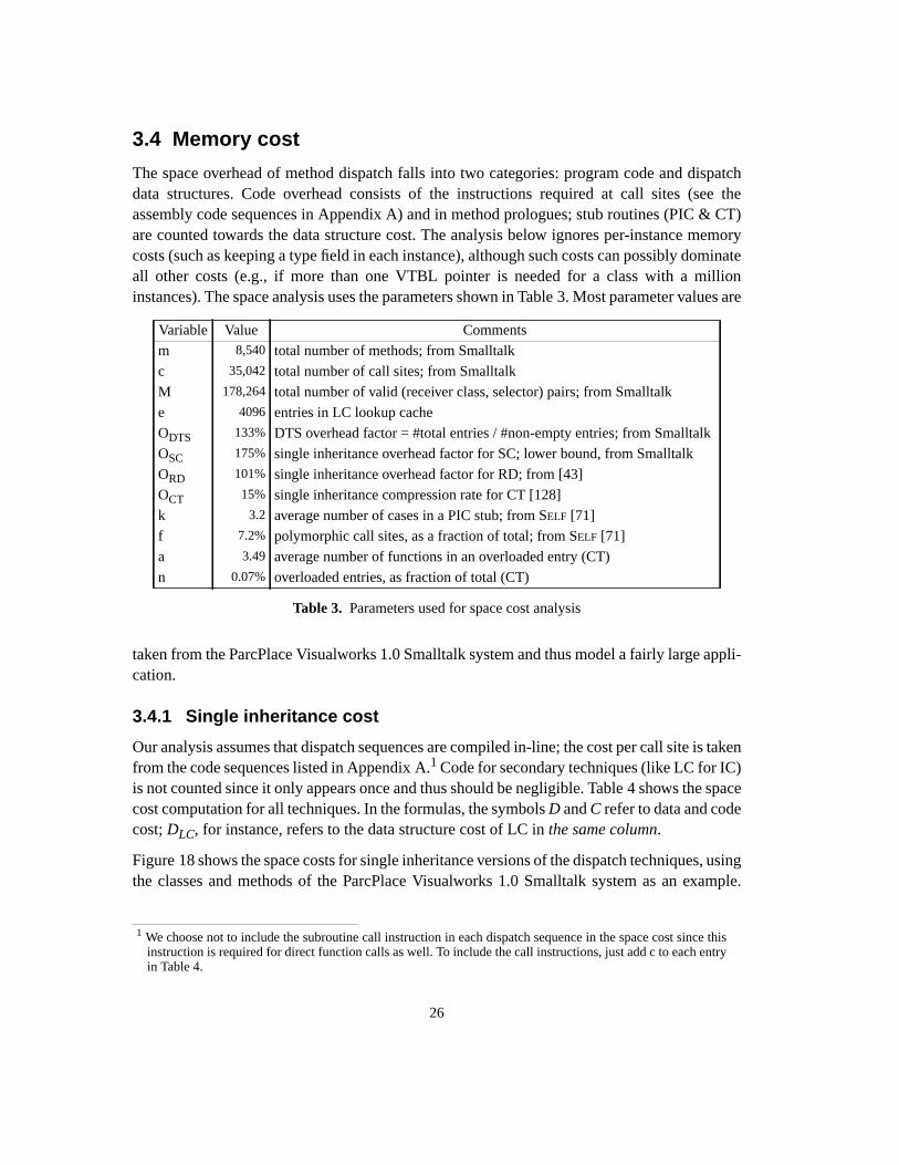
26

3.4 Memory cost

The space overhead of method dispatch falls into two categories: program code and dispatchdata structures. Code overhead consists of the instructions required at call sites (see theassembly code sequences in Appendix A) and in method prologues; stub routines (PIC & CT)are counted towards the data structure cost. The analysis below ignores per-instance memorycosts (such as keeping a type field in each instance), although such costs can possibly dominateall other costs (e.g., if more than one VTBL pointer is needed for a class with a millioninstances). The space analysis uses the parameters shown in Table 3. Most parameter values are

taken from the ParcPlace Visualworks 1.0 Smalltalk system and thus model a fairly large appli-cation.

3.4.1 Single inheritance cost

Our analysis assumes that dispatch sequences are compiled in-line; the cost per call site is takenfrom the code sequences listed in Appendix A.1 Code for secondary techniques (like LC for IC)is not counted since it only appears once and thus should be negligible. Table 4 shows the spacecost computation for all techniques. In the formulas, the symbolsD andC refer to data and codecost;DLC, for instance, refers to the data structure cost of LC inthe same column.

Figure 18 shows the space costs for single inheritance versions of the dispatch techniques, usingthe classes and methods of the ParcPlace Visualworks 1.0 Smalltalk system as an example.

1 We choose not to include the subroutine call instruction in each dispatch sequence in the space cost since thisinstruction is required for direct function calls as well. To include the call instructions, just add c to each entryin Table 4.

Variable Value Comments

m 8,540 total number of methods; from Smalltalk

c 35,042 total number of call sites; from Smalltalk

M 178,264 total number of valid (receiver class, selector) pairs; from Smalltalk

e 4096 entries in LC lookup cache

ODTS 133% DTS overhead factor = #total entries / #non-empty entries; from Smalltalk

OSC 175% single inheritance overhead factor for SC; lower bound, from Smalltalk

ORD 101% single inheritance overhead factor for RD; from [43]

OCT 15% single inheritance compression rate for CT [128]

k 3.2 average number of cases in a PIC stub; from SELF [71]

f 7.2% polymorphic call sites, as a fraction of total; from SELF [71]

a 3.49 average number of functions in an overloaded entry (CT)

n 0.07% overloaded entries, as fraction of total (CT)

Table 3. Parameters used for space cost analysis

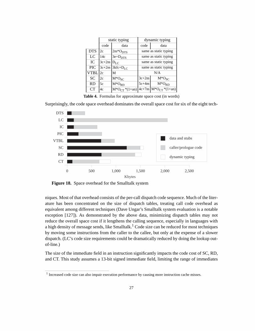
27

Surprisingly, the code space overhead dominates the overall space cost for six of the eight tech-

niques. Most of that overhead consists of the per-call dispatch code sequence. Much of the liter-ature has been concentrated on the size of dispatch tables, treating call code overhead asequivalent among different techniques (Dave Ungar’s Smalltalk system evaluation is a notableexception [127]). As demonstrated by the above data, minimizing dispatch tables may notreduce the overall space cost if it lengthens the calling sequence, especially in languages witha high density of message sends, like Smalltalk.1 Code size can be reduced for most techniquesby moving some instructions from the caller to the callee, but only at the expense of a slowerdispatch. (LC’s code size requirements could be dramatically reduced by doing the lookup out-of-line.)

The size of the immediate field in an instruction significantly impacts the code cost of SC, RD,and CT. This study assumes a 13-bit signed immediate field, limiting the range of immediates

1 Increased code size can also impair execution performance by causing more instruction cache misses.

static typing dynamic typingcode data code data

DTS 2c 2m*ODTS same as static typing

LC 14c 3e+DDTS same as static typing

IC 3c+2m DLC same as static typing

PIC 3c+2m 3kfc+DLC same as static typing

VTBL 2c M N/A

SC 2c M*OSC 3c+2m M*OSC

RD 5c M*ORD 5c+4m M*ORD

CT 4c M*OCT *(1+an) 4c+7m M*OCT *(1+an)

Table 4. Formulas for approximate space cost (in words)

CT

RD

SC

VTBL

PIC

IC

LC

DTS

0 500 1,000 1,500 2,000 2,500

Kbytes

data and stubs

caller/prologue code

dynamic typing

Figure 18. Space overhead for the Smalltalk system

28

to -4096..4095.1 The Smalltalk system measured had 5087 selectors, and thus the selectornumber fits into an immediate. SC needs only one instruction to load the selector code into aregister (see Table A-4), but RD takes two instructions for the same action because the selectornumber is a memory address, pointing to the beginning of a selector table. The same phenom-enon increases the method prologue overhead in both RD and CT.2 In RD, the reduction in datastructure size relative to SC is almost offset by a corresponding increase in code size. The datain Figure 18 are thus relative to the processor architecture. For example, for an architecture withlarger immediates (or for smaller applications), CT’s space advantage over VTBL woulddouble. Of course, the data also depends on application characteristics such as the proportion ofcall sites versus number of classes, selectors, and methods.

Given these admonitions, IC and PIC apparently combine excellent average speed with lowspace overhead. The bounded lookup time of SC and RD is paid for with twice as muchmemory; VTBL is about one third smaller than those two. CT’s small data structure size isoffset by its code cost.

VTBL, RD, and SC require significantly more data space than DTS because they duplicateinformation. Each class stores all the messages itunderstands, instead of all the messages itdefines. For example, in the Smalltalk system a class inherits 20 methods for each one it defines[40], so the number of entries stored in the class’ dispatch table increases by a factor of 20.

Dynamic typing makes a relatively small difference in space cost. Dynamic techniques have noextra overhead because each dispatch already contains a run-time check to test for the cache hit.Static techniques3 perform the run-time type check in the method prologue, so the overheadgrows linearly with the number of defined methods, which is much smaller than the number ofcall sites.

3.4.2 Multiple inheritance cost

The space overhead of multiple inheritance is more difficult to measure than single inheritancespace cost. For VTBL-MI, the call sequence consists of two extra instructions, and virtual func-tion tables have an extra entry which stores the object pointer adjustment (see Section 3.1.2).This brings the code cost to 4c, and the data structure cost to 2M. However, every time a classinherits from an ancestor though different paths (the “diamond” problem), all functions inher-ited through that ancestor are stored twice (with different adjustments). This overhead dependsentirely on the way multiple inheritance is used and is not quantifiable without appropriate codemetrics. In [43], we calculated this overhead for two class libraries that use multiple inheritanceextensively. The generated tables stored, respectively, 215% and 330% of the entries that a

1 The size of immediates varies from architecture to architecture: for example, SPARC has 13 bits, Alpha 8 bits,and MIPS 16 bits.

2 Here the crucial quantity is the number of bits necessary to represent acid (16 bits for the Smalltalk example).For the same reason, CT’s dynamic typing cost is higher.

3 Excluding VTBL, which only works for statically-typed languages.

29

single table would use (assuming non-hard-coded offsets). Finally, the overhead of havingmultiple table pointers in each object can only be calculated for individual program runs, sinceit depends on the number of object allocated.

Static techniques (SC, RD) with one table per object (or per message selector), exhibit thecompiled code cost of dynamic techniques, plus an additional overhead because multiple inher-itance hierarchies generate tables that are harder to compress. For SC, multiple inheritanceintroduces conflicts between selector colors that are hard to deal with and that substantiallyincrease the number of empty entries [9]. For two libraries with extensive use of multiple inher-itance (Every class has on average two parent classes), the resulting tables contained 71% and74% empty entries. For RD, multiple inheritance causes more irregular empty regions to appearin the original two-dimensional table, which makes the rows harder to fit tightly together. RD ismore robust than both VTBL-MI and SC, however, since the resulting tables contained only 9%and 29% empty entries (see Section 4.3.3).

3.5 Programming environment aspects

The choice of a dispatch technique is influenced by considerations other than space cost andexecution speed (discussed in Section 5). Code organization and demands put upon theprogramming environment can preclude some techniques from being used. The followingaspects, though non-comprehensive, give an idea of the issues involved:

• Responsiveness. Some static techniques are less suitable for interactive programmingenvironments that demand a high level or responsiveness (i.e., immediate feedback toprogramming changes). Most static techniques need to recompute some data structuresafter a programming change. For example, introducing a new method name forces VTBLto rearrange the dispatch table of the affected class and all its subclasses. SC, RD and CTeven have to completely recompute their tables from scratch (except in rare cases, e.g., ifthe new method fits into an empty slot in the dispatch table). For the Smalltalk system,complete recomputation can take hours for SC, and seconds for RD and CT.

• Support for run-time extensibility. Many static techniques (e.g., SC, RD, CT) presumeknowledge of the entire program, i.e., knowledge of all classes and methods. With dynamiclink libraries (DLL), the complete set of classes and methods is not known until run timesince the classes contained in dynamic libraries are unknown until they are loaded atprogram start-up time or later during the execution of the program. Thus, these techniqueshave to recompute the dispatch data structures each time a new library is dynamicallyloaded.

• Sharing code pages. Some operating systems (e.g., Unix) allow processes executing thesame program to share the memory pages containing the program’s code. With shared codepages, overall memory usage is reduced since only one copy of the program (or sharedlibrary) need be in memory even if it is used concurrently by many different users. For code

30

to be shared, most operating systems require the code pages to be read-only, thusdisallowing techniques that modify program code on-the-fly (e.g., IC and PIC).

Many of the dispatch techniques discussed here can be modified to address problems such asthose outlined above. For example, static techniques can be made more incremental by intro-ducing extra levels of indirection at run-time (e.g., by loading the selector number rather thanembedding it in the code as a constant), usually at a loss in dispatch performance. For this study,only the simplest and fastest version of each technique was considered, but any variant can beanalyzed using the same evaluation methodology.

3.6 Summary

Instructions (in particular, per-call code) can contribute significantly to the overall spacerequirements of message dispatch. In our example system, many techniques spend morememory on dispatch code sequences than on dispatch data structures. Thus, minimizingdispatch table size may not always be the most effective way to minimize the overall space cost,and may in some cases even increase the overall space cost.

Run-time system constraints can limit the choice of dispatch techniques available to practitio-ners. For static caching techniques, table construction time can be prohibitive. Inline cachingtechniques require modifiable code.

31

4 Row displacement compression“I visualize structures, graphs, data structures.Its seems to come a easier than a lot of otherthings”

Robert E. Tarjan [115]

Table-based dispatch is attractive because its cost is bound by a constant. The critical path ofselector table indexing (STI), the simple, fast, but memory-greedy static technique, consists oftwo dependent loads and an indirect branch instruction. On older processors, this sequencetakes about 5 cycles, 4 if the branch delay slot can be filled. On newer processors, the sequencetakes in the worst case (branch mispredict), two load latencies plus a branch mispredictionpenalty (about 8 cycles on the P96 processor used as state-of-the-art representative inSection 6).

Therefore, the simplest form of table-based dispatch is fast and reliable. Its main problem is itsprohibitive memory cost. A straightforward implementation uses a two-dimensional table ofsize S * C, where S is the number of message selectors (10K for SELF) and C the number ofclasses (1.8K in SELF). For mature programming environments, this table simply takes toomuch memory (18M addresses = 72Mbytes on a SPARC). Since each class responds to only afraction of all message selectors (typically between 2% and 10%), the table could be broughtdown to a reasonable size, if only the non-null entries were stored (1M addresses for SELF =4Mbytes on a SPARC).

In statically typed languages like C++ or Java, virtual function tables (VTBL) avoid storage ofnull entries because of a numbering scheme that appends new entries to an existing table. VTBLdispatch takes no more instructions than STI. With single parent class inheritance, this schemeis optimal. No null entries are stored. When multiple inheritance is employed, the numberingscheme does not guarantee zero overhead because of the necessity to merge two or more tables.However, table compression becomes expedient only with high occurrence of multiple inherit-ance. Multiple inheritance incurs a small overhead of two extra instructions in the dispatchsequence, but these instructions are independent of the critical path instructions, and can there-fore be hidden in the extra instruction issue of a superscalar processor1.

In dynamically typed languages, each class must respond to all messages, since the compilerdoes not guarantee that a particular object implements a message sent to it. This “message notunderstood” error is caught at run time. Semantically speaking, the default implementation ofall messages isMessageNotUnderstood. Table compression of dispatch tables aims to storeonly the non-default implementations (the 2% to 10% non null entries in the STI table).Absence of an implementation must be detected by the dispatch code at run time, and trigger theinvocation ofMessageNotUnderstood. For the table-based dispatch we discuss in this chapter,

1 However, the dependency of those instructions on the availability of the receiver’s address can incur delays in some programs(see section 6.4.2)

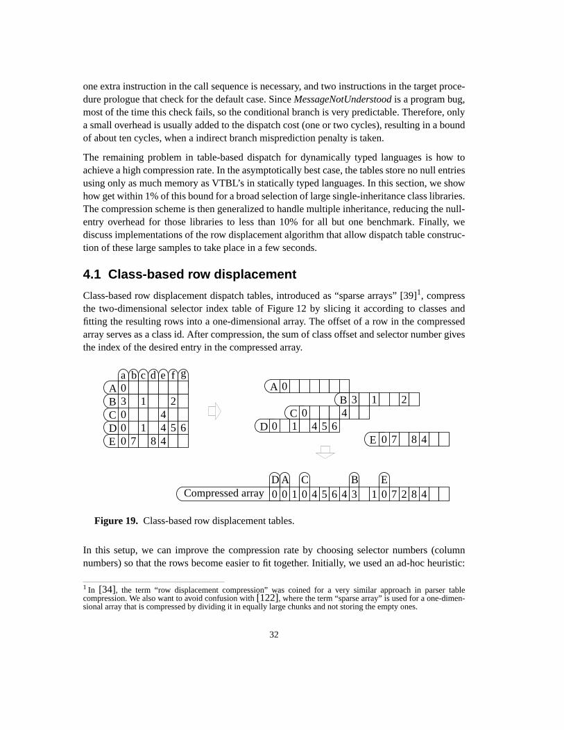
32

one extra instruction in the call sequence is necessary, and two instructions in the target proce-dure prologue that check for the default case. SinceMessageNotUnderstood is a program bug,most of the time this check fails, so the conditional branch is very predictable. Therefore, onlya small overhead is usually added to the dispatch cost (one or two cycles), resulting in a boundof about ten cycles, when a indirect branch misprediction penalty is taken.

The remaining problem in table-based dispatch for dynamically typed languages is how toachieve a high compression rate. In the asymptotically best case, the tables store no null entriesusing only as much memory as VTBL’s in statically typed languages. In this section, we showhow get within 1% of this bound for a broad selection of large single-inheritance class libraries.The compression scheme is then generalized to handle multiple inheritance, reducing the null-entry overhead for those libraries to less than 10% for all but one benchmark. Finally, wediscuss implementations of the row displacement algorithm that allow dispatch table construc-tion of these large samples to take place in a few seconds.

4.1 Class-based row displacement

Class-based row displacement dispatch tables, introduced as “sparse arrays” [39]1, compressthe two-dimensional selector index table of Figure 12 by slicing it according to classes andfitting the resulting rows into a one-dimensional array. The offset of a row in the compressedarray serves as a class id. After compression, the sum of class offset and selector number givesthe index of the desired entry in the compressed array.

In this setup, we can improve the compression rate by choosing selector numbers (columnnumbers) so that the rows become easier to fit together. Initially, we used an ad-hoc heuristic:

1 In [34], the term “row displacement compression” was coined for a very similar approach in parser tablecompression. We also want to avoid confusion with[122], where the term “sparse array” is used for a one-dimen-sional array that is compressed by dividing it in equally large chunks and not storing the empty ones.

A C B E

Figure 19. Class-based row displacement tables.

Aa0

b c d e f g

B 3 1 2C 0 4D 0 1 4 5 6E 0 7 8 4

A 0B 3 1 2

C 0 4D 0 1 4 5 6

E 0 7 8 4

Compressed array0 0 1 0 4 5 6 0 7 2 8 414 3D

33

we numbered the message selectors defined in meta-classes in the Smalltalk library first. Theseclasses are numerous (half of the total number of classes), and each one understands a largenumber of messages (300 on average, compared to 160 for regular classes), taken from a limitedset of selectors (about 1300, compared to 4000 for regular classes). Therefore, first numberingthose selectors sequentially results in a large number of rows with densely packed entries,making the fitting process efficient. After fitting meta-classes, the wide, sparsely filled regularclass rows caused a resulting overhead of 40% [39].

We then designed a heuristic based on a generalization of this ad-hoc rule for Smalltalk classes.This results in a better compression rate, but 33% of the table still stores undefined entries [40].

4.2 Selector-based row displacement

Selector-based row displacement functions the same way as class-based row displacement, butwe slice the two-dimensional table up according to selectors, instead of classes. Figure 20 illus-trates the process on the same class hierarchy as used in Figure 19: the compression algorithmworks on thetransposed selector index table. At run time, the lookup process is similar, with therole of classes and selectors reversed. However, for the “message not understood”-test, themethod still tests whether the called and definedselector are equal.

In this setup, the numbering of classes determines the shape of the rows to be fitted in thecompressed array. This simple change dramatically improves the fill rate (i.e., reduces the size)of the compressed array. Selector-based tables have less overhead than class tables for tworeasons: their row size distribution makes it easier to tightly pack rows together and theirmessage definitions cluster in a more regular way under inheritance, which reduces the amountof gaps within rows. Both of these aspects can be exploited by an appropriate class numberingscheme, as explained in the next sections.

fca b d e

Figure 20. Selector-based row displacement tables

a 0 3 0 0 0b 7c 1 1d 8e 4 4 4f 2 5g 6

a 0 3 0 0 0b 7

c 1 1d 8

e 4 4 4f 2 5

g 6

A B C D E

Compressed array0 3 0 0 0 7 1 8 1 4 4 2 6 5g4

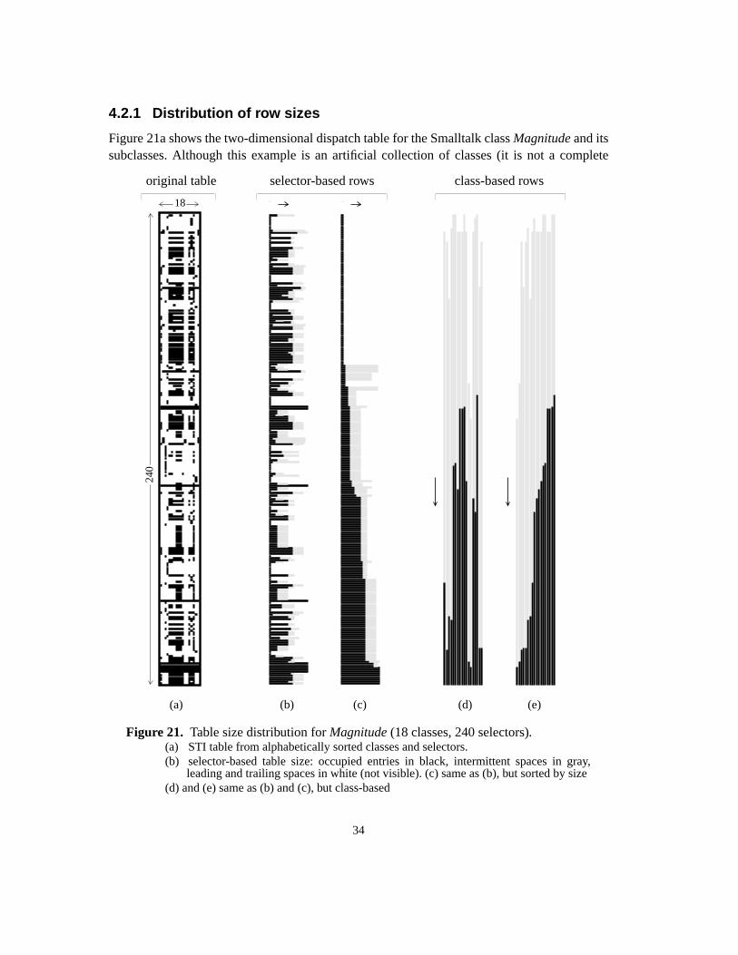
34

4.2.1 Distribution of row sizes

Figure 21a shows the two-dimensional dispatch table for the Smalltalk classMagnitude and itssubclasses. Although this example is an artificial collection of classes (it is not a complete

240

18

(a) (b) (c) (d) (e)

Figure 21. Table size distribution forMagnitude(18 classes, 240 selectors).

original table selector-based rows class-based rows

(a) STI table from alphabetically sorted classes and selectors.(b) selector-based table size: occupied entries in black, intermittent spaces in gray,

leading and trailing spaces in white (not visible). (c) same as (b), but sorted by size(d) and (e) same as (b) and (c), but class-based

35

program), it does demonstrate the characteristic size distributions found in larger, realisticsamples.

To begin with, the number of classes is much smaller than the number of message selectors.Therefore the average size of class-based rows will be much larger than that of selector-basedrows. In [41], we found that row displacement compression works better, in general, with manysmall rows than with few large ones. Thus a selector-based table is likely to be compressedbetter than a class-based table. Although not all the cases we tested exhibit as large a differenceasMagnitude, usually the number of selectors is at least twice the number of classes. Thisasymmetry accounts for part of the better fill rate of selector tables.

In addition to the average row size, thedistribution of row sizes also has an impact on the fillrate. Figure 21b illustrates why. Figure 21b is constructed from 21a by squeezing occupiedentries (in black) together.1 The width of the black rows thus indicates the number of occupiedentries of that row. The gray area represents unoccupied space that is not leading or trailing therow, but is enclosed by occupied entries to its left and right. Thus black and gray area togethergive the maximum space that a row can occupy under row displacement. We call this quantitythe width of a row vector. The white area is free because leading and trailing empty space canoverlap with other rows. Figure 21c is the same as 21b, but with selectors reordered by size tobetter show the distribution. Figures 21d and 21e show the same for a class-based table, rotated90 degrees.

The black area represents a lower bound on the size of the compressed array; black and graytogether represent an upper bound. If all rows were placed consecutively, the size of thecompressed array would be the sum of all the row widths. Gray area can thus be consideredpotential overhead.

When comparing Figure 21c with Figure 21e, it becomes clear why a selector-based table doesbetter than a class-based table: almost one third of the selector-based rows have only one occu-pied entry. These ultra-small rows are ideal to fill up gaps left by other rows. Class-based rowson the other hand have a minimal size of nine. The difference tends to get worse as librariesgrow larger. For example, in VisualWorks 1.0 every class understands at least 100 messages, but45% of the messages are only known by one class, and another 39% by less than ten classes.Furthermore, the potential overhead (gray area) for the selector-based table in Figure 21 ismuch smaller than that of a class-based table. Thus a selector-based table has less area to fill up,and better material to fill it up with.

Without further efforts, selector-based row displacement already outperforms the most sophis-ticated class-based row displacement schemes. ForMagnitude, the best fill rate reached in [40]is 80%, while the structure shown in Figure 21b gives a compressed array that is 87% occupied.This difference becomes larger as class libraries grow larger, as we will see in section 4.3.

1 This figure does not correspond to an actual data structure in the compression algorithm. It is given only to illustrate thecharacteristics of rows in a selector-based table.

36

4.2.2 Fitting order

The previous section demonstrated that class- and selector-based tables have different row sizedistributions. This section and the next explains how to exploit this difference to its fullest in anactual implementation.

Since it is not practical to look for the best possible configuration, i.e., to look for offsets thatminimize total overhead,1 we fill the compressed array in one pass. Rows are inserted into thefirst place that fits, but we still have the freedom to choose the order in which rows are inserted.Figure 21b shows the alphabetical order, which is an arbitrary one from an algorithmic perspec-tive; as mentioned before, it achieves 87% fill rate. Figure 21c shows the rows ordered by size.We start with the largest rows and work from there to the smaller ones. Intuitively, this arrange-ment gives smaller rows a better chance to fill up holes left by bigger ones. ForMagnitude thefill rate does indeed improve to 93%. Larger samples exhibit a smaller difference but consis-tently favor the size-ordered scheme.

Surprisingly, sorting rows according to descending size does not slow down the algorithm.Because the time needed to fit all rows is proportional to the average number of unoccupiedentries that is checked before a fitting space is found, a denser compression is reached in ashorter time. Thus the gain in speed caused by the better fill rate compensates for the extra timeneeded to sort rows.

4.2.3 Class numbering for single inheritance

Now that we have established the ordering of selectors, this section will show how classes canbe numbered to enhance the fill rate further.

If we look back at Figure 20, exchanging column D and C makes the fitting process trivial,because no gaps are left in any rows. All empty entries are found either in the beginning or theend of a row. Merely placing these rows back to back in the compressed array solves thecompression problem. A class numbering scheme that minimizes the number of gaps in aselector-based table is illustrated in Figure 22.

The aim is to make sure that all classes that understand a certain message have consecutivenumbers. Our scheme numbers classes by traversing the inheritance tree in depth-first pre-order. This numbering scheme ensures that every subtree in the inheritance structure corre-sponds to a consecutive block of class numbers. Since most message selectors are understoodby exactly a subtree of classes, most rows in the selector-based table consist of exactly oneconsecutive block of occupied entries. For the single-inheritance hierarchy of Figure 22, thenew class numbering reduces the number of gaps from four to one. The only selector with a gapin its row ise, becausee is defined separately in two classes (D andF), without being definedin a common super class.

1 This problem is NP-complete[121] and thus takes too long to solve, or even to approximate[41].

37

Figure 23 shows the effect of the numbering scheme onMagnitude. Figure 23a shows aselector-based table, with the rows ordered in increasing size. 35% of the total area is potentialoverhead (gray). As mentioned before, this table resulted in 93% fill rate, so 7% of the 35%became real overhead. After renumbering classes, only 1.6% potential overhead is left(Figure 23b), and compression reduces this gray area to 0.5% real overhead. Out of an arraywith 1388 entries, only 3 are unoccupied, and even these gaps are caused by contention overrow offsets by one-entry rows, not by true fitting conflicts (remember that all rows need to haveunique offsets in the compressed array). Later, in section 4.3, we will present compressionresults for several other single inheritance class libraries.

4.2.4 Class numbering for multiple inheritance

The depth-first numbering scheme can easily be applied to a multiple inheritance class library.The only difference to single inheritance is that a class with more than one direct super class(a.k.a. base class) will be visited more than once. Since a class is numbered the first time it isencountered, its number will depend on the order in which subclasses are traversed. We foundthat an essentially random choice is good enough if multiple inheritance is not used frequently,as in theUnidraw/Interviews sample of section 4.3.

However, if multiple inheritance is used extensively, it is worthwhile to spend time on a betternumbering scheme. We construct a single-inheritance hierarchy from the multiple inheritancehierarchy by considering only the dominant super class link. The dominant super class is theclass that makes the largest contribution to the dispatch table. For example, in Figure 24, classB is the dominant super class of classE becauseE inherits more messages throughB than

bcf d

A a

B C

eD gE edF

G

A

B C

D E F

G

0

1

2

3 4

5 6

aA B C D E

0 1 0 1 0

bcdefg

F

0

G

0

2

aA B CD E

0 1 01 0

bc 3 3

d 5 5

e 7

f 4 4

g 9

F

0

6

8

G

0

2

0 1 42 5 63

Figure 22. Alphabetic and depth-first class numbers

38

through any other of its super classes. It is easy to see why this choice produces the fewestnumber of gaps: if a class inherits from several classes, it will be numbered out of sequence inthe subtrees of all classes except one.1 Thus it will cause a gap in the rows of all message selec-

1 Exception: if a class number appears at the edge of a consecutive block it may, by pure chance, be adjacent to the number ofanother of its base classes.

(a) (b)

Figure 23. Magnitude: selector-based tableswith classes numbered:(a) alphabetically(b) depth-first preorder

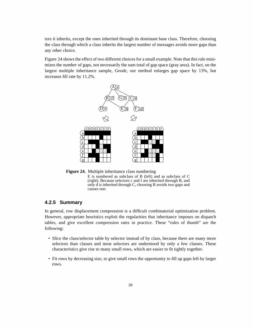
39

tors it inherits, except the ones inherited through its dominant base class. Therefore, choosingthe class through which a class inherits the largest number of messages avoids more gaps thanany other choice.

Figure 24 shows the effect of two different choices for a small example. Note that this rule mini-mizes thenumber of gaps, not necessarily the sum total of gap space (gray area). In fact, on thelargest multiple inheritance sample,Geode, our method enlarges gap space by 13%, butincreases fill rate by 11.2%.

4.2.5 Summary

In general, row displacement compression is a difficult combinatorial optimization problem.However, appropriate heuristics exploit the regularities that inheritance imposes on dispatchtables, and give excellent compression rates in practice. These “rules of thumb” are thefollowing:

• Slice the class/selector table by selector instead of by class, because there are many moreselectors than classes and most selectors are understood by only a few classes. Thesecharacteristics give rise to many small rows, which are easier to fit tightly together.

• Fit rows by decreasing size, to give small rows the opportunity to fill up gaps left by largerrows.

Figure 24. Multiple inheritance class numbering

aA B CD E

0 1 01 0

bcd 5 5

efg

F

0

6

8

G

0

bcf d

aA B CD E

0 1 01 0

bc 3 3 3

d 55

e 7

f 4 4 4

g 9

A a

B C

eD gE edF

F

0

6

8

G

G

0

2

E is numbered as subclass of B (left) and as subclass of C(right). Because selectors c and f are inherited through B, andonly d is inherited through C, choosing B avoids two gaps andcauses one.

40

• Number classes according to a depth-first pre-order traversal of the inheritance structure, toforce occupied entries to cluster together.

• For multiple inheritance libraries: ignore all base classes in the numbering scheme, exceptthe base class which understands the largest number of messages.

4.3 Compression results

In this section we compare four variants of selector-based row displacement with other table-based message dispatch techniques on a number of large class libraries. We will first discuss theway space overhead is calculated, then briefly outline the test samples, and finally discuss theresults.

4.3.1 Methodology

To evaluate the effectiveness of table compression techniques, we measure how close the tablesize approachesM: the sum, over all classes, of the number of messages understood by a class.This sum is the total of legitimate class-selector combinations of a class library. A messagedispatch technique that finds a method in a constant, small amount of time needs to store eachone of these combinations. We define thefill rate of a technique asM divided by the actualnumber of entries for which storage is allocated. For instance, dividingM by the product of thenumber of classes and the number of selectors calculates the fill rate of the two-dimensionalclass/selector table employed by STI (see Section 3.3.1).

Selector coloring (SC) [38][9] expresses table compression as a graph coloring problem. Thegraph represents selectors by nodes. An edge between two nodes means that the correspondingtwo selectors occur in the same class. The aim of the coloring algorithm is to assign a color toeach node of the graph so that adjacent nodes have different colors, with as few colors aspossible. What this technique boils down to in terms of the two-dimensional dispatch table isthe following: selector coloring compresses the table by overlapping columns. Every selector isassigned a column number. Two selectors can share a column if none of their occupied entrieshave the same index (i.e., they do not occur together in any class).

A lower bound for the number of columns is the size of the largest row. This row correspondsto the class that understands the largest number of messages. Multiplying this number by thetotal number of classes gives a lower bound to the number of entries of the resulting data struc-ture. DividingM by this lower bound then gives an upper bound to the fill rate, which is thequantity we show under column SC. It is independent of the coloring algorithm used1.

Virtual function tables (VF) [32], the preferred implementation of message dispatch in C++compilers [53], have no overhead for single inheritance class libraries. Multiple inheritanceincurs space overhead because every base class requires its own virtual function table, dupli-

1 Since graph coloring is NP-complete, optimal coloring schemes are approximated by polynomial-time algorithms.

41

cating entries that are common to two or more base classes. For example, in Figure 24, classEhas two virtual function tables, both of which storea. The size of a class’s virtual function tablesequals the sum of its parents’ virtual tables plus the number of newly defined (not overridden)messages.

For class-based row displacement (CR) we took the fill rate reached by the heuristic describedin [40]. This heuristic performed best on all samples except Object, where Horn’s algorithmreached a better fill rate (67% instead of 64%).

Selector-based row displacement is shown for three variations in class numbering: alphabetical(AL), depth-first pre-order traversal for a single-inheritance hierarchy (SI), and depth-first pre-order traversal for a multiple-inheritance hierarchy (MI). Fill rates are shown for the fastestimplementation of row displacement, which trades some fitting tightness for speed, asexplained in section 4.4.1.

4.3.2 Samples

We choose sample class libraries taken from real systems for three reasons: it facilitatescomparison with other methods, it eliminates the extra step of verifying whether the real worldbehaves the same as the artificial samples, and as an aside it gives us the opportunity to gathersome statistics from programs with hundreds of classes, which is interesting in its own right.

On the other hand, the data points do not cover the realm of possible class libraries as evenly aswe would wish. Self-contained programs are usually large, consisting of several hundredclasses. To get an impression of how the different techniques behave on smaller examples, wealso used subsets of the Smalltalk inheritance structure. These are the first six samples ofTable 5. The next six samples are comprised of all the classes of different Smalltalk images:Parcplace Visualworks 1.0 and 2.0, Digitalk Smalltalk 2.0 and 3.0, and VisualAge Smalltalk2.0, kernel and complete library. The next two samples are NextStep, written in Objective-C,and the SELF system 4.0. The two C++ samples are the ET++ Application Framework [131] andUnidraw/InterViews [92]. Only the latter uses multiple inheritance, in only 10 classes (theaverage number of base classes is smaller than 1 because 147 of the classes in this library haveno base class). The last two samples are from LOV, a proprietary language based on Eiffel.These two make extremely heavy use of multiple inheritance: on averageevery class inheritsfrom two super classes.

4.3.3 Compression results

Table 5 shows the result of our measurements. Selector-based row displacement performs verywell on single-inheritance samples (all samples with “-” in column P). Fill rates are higher than99.5% for all self-contained examples, and more than 98% for the smaller ones. The techniquescales up well: contrary to selector coloring and class-based row displacement, compressionimproves as libraries grow in size. The class numbering scheme is partly responsible for this

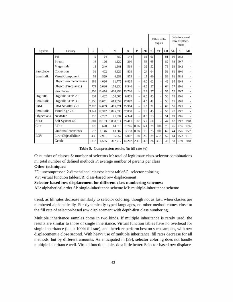
42

trend, as fill rates decrease similarly to selector coloring, though not as fast, when classes arenumbered alphabetically. For dynamically-typed languages, no other method comes close tothe fill rate of selector-based row displacement with depth-first class numbering.

Multiple inheritance samples come in two kinds. If multiple inheritance is rarely used, theresults are similar to those of single inheritance. Virtual function tables have no overhead forsingle inheritance (i.e., a 100% fill rate), and therefore perform best on such samples, with rowdisplacement a close second. With heavy use of multiple inheritance, fill rates decrease for allmethods, but by different amounts. As anticipated in [39], selector coloring does not handlemultiple inheritance well. Virtual function tables do a little better. Selector-based row displace-

Other tech-niques

Selector-basedrow displace-

ment

System Library C S M m P 2D SC VF CR AL SI MI

Set 9 94 450 144 - 53 65 - 81 90 98.3 -

Stream 16 126 1,122 210 - 56 65 - 82 93 99.7 -

Magnitude 18 240 1,381 568 - 32 52 - 78 93 99.2 -

Parcplace Collection 51 402 4,926 805 - 24 64 - 59 81 99.0 -

Smalltalk VisualComponent 53 529 4,253 875 - 15 60 - 56 91 98.8 -

Object w/o metaclasses 383 4,026 61,775 6,835 - 4.0 62 - 48 95 99.4 -

Object (Parcplace1) 774 5,086 178,230 8,540 - 4.5 57 - 64 77 99.6 -

Parcplace2 1,956 13,474 608,456 23,720 - 2.3 57 - 55 72 99.7 -

Digitalk Digitalk ST/V 2.0 534 4,482 154,585 6,853 - 6.5 43 - 56 78 99.6 -

Smalltalk Digitalk ST/V 3.0 1,356 10,051 613,654 17,097 - 4.5 42 - 50 71 99.8 -

IBM IBM Smalltalk 2.0 2,320 14,009 485,321 25,994 - 1.5 32 - 63 56 99.5 -

Smalltalk VisualAge 2.0 3,241 17,342 1,045,333 37,058 - 1.9 43 - 55 47 99.7 -

Objective-C NextStep 310 2,707 71,334 4,324 - 8.5 53 - 51 89 99.6 -

SELF Self System 4.0 1,801 10,103 1,038,514 29,411 1.02 5.7 60 - 47 67 99.7 99.8

C++ ET++ 370 628 14,816 1,746 0.76 6.4 29 100 78 46 97.6 97.6

Unidraw/Interviews 613 1,146 13,387 3,153 0.78 1.9 23 100 62 44 95.6 95.7

LOV Lov+ObjectEditor 436 2,901 36,052 5,007 1.78 2.9 29 46.5 52 64 75.2 91.1

Geode 1,318 6,555 302,717 14,202 2.11 3.5 26 30.3 45 58 57.9 70.8

Table 5. Compression results (in fill rate %)

C: number of classes S: number of selectors M: total of legitimate class-selector combinationsm: total number of defined methods P: average number of parents per classOther techniques:2D: uncompressed 2-dimensional class/selector tableSC: selector coloringVF: virtual function tablesCR: class-based row displacementSelector-based row displacement for different class numbering schemes:AL: alphabetical order SI: single-inheritance scheme MI: multiple-inheritance scheme

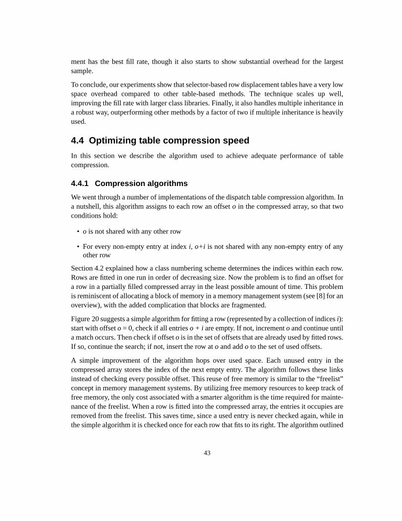
43

ment has the best fill rate, though it also starts to show substantial overhead for the largestsample.

To conclude, our experiments show that selector-based row displacement tables have a very lowspace overhead compared to other table-based methods. The technique scales up well,improving the fill rate with larger class libraries. Finally, it also handles multiple inheritance ina robust way, outperforming other methods by a factor of two if multiple inheritance is heavilyused.

4.4 Optimizing table compression speed

In this section we describe the algorithm used to achieve adequate performance of tablecompression.

4.4.1 Compression algorithms

We went through a number of implementations of the dispatch table compression algorithm. Ina nutshell, this algorithm assigns to each row an offseto in the compressed array, so that twoconditions hold:

• o is not shared with any other row

• For every non-empty entry at indexi, o+i is not shared with any non-empty entry of anyother row

Section 4.2 explained how a class numbering scheme determines the indices within each row.Rows are fitted in one run in order of decreasing size. Now the problem is to find an offset fora row in a partially filled compressed array in the least possible amount of time. This problemis reminiscent of allocating a block of memory in a memory management system (see [8] for anoverview), with the added complication that blocks are fragmented.

Figure 20 suggests a simple algorithm for fitting a row (represented by a collection of indicesi):start with offseto = 0, check if all entrieso + i are empty. If not, incremento and continue untila match occurs. Then check if offseto is in the set of offsets that are already used by fitted rows.If so, continue the search; if not, insert the row ato and addo to the set of used offsets.

A simple improvement of the algorithm hops over used space. Each unused entry in thecompressed array stores the index of the next empty entry. The algorithm follows these linksinstead of checking every possible offset. This reuse of free memory is similar to the “freelist”concept in memory management systems. By utilizing free memory resources to keep track offree memory, the only cost associated with a smarter algorithm is the time required for mainte-nance of the freelist. When a row is fitted into the compressed array, the entries it occupies areremoved from the freelist. This saves time, since a used entry is never checked again, while inthe simple algorithm it is checked once for each row that fits to its right. The algorithm outlined

44

so far comprises the SIO algorithm in Table 6, which stands for “singly-linked freelist withindex-ordered single-entry rows”. We will explain the latter denotation later.

Although rows can be arbitrarily fragmented in principle, in practice they usually consist of alarge block with a few “satellite” pieces if an adequate class numbering scheme is used, asdemonstrated in section 4.2. Therefore, smarter, faster allocation schemes can be adapted frommemory management techniques that deal with variable sized blocks. The key trick is to testfirst for the largest consecutive block of a row, and to organize the freelist so that one can easilyenumerate free blocks with a certain minimum size. Then the highly fragmented free spacewhich tends to accumulate in the filled portion of the compressed array is skipped when fittinglarge rows. In [40], we implemented and tested an algorithm (BBBF) built around a freelistwhich was actually a binary search tree, ordered by size. The main disadvantage of this tech-nique is that free blocks must have a size of six or more consecutive entries or they cannot belinked into the tree. Blocks of size five and smaller are not linked at all. This not only compli-cates the maintenance of the free list, but, more importantly, renders the algorithm impracticalfor selector-based rows. As demonstrated in section 4.2, the majority of selector-based rows issmaller than six, whereas class-based rows have a minimum size far exceeding that. The algo-rithm in [40] is also more general than necessary, since it can deal with arbitrarily large blocks.The maximum block size in this particular problem is equal to the size of the largest row, whichis the number of selectors in the system (10K in Self, a large system).1

Here we use the simpler approach of linking together equally sized blocks. An array indexed byblock size contains pointers to the beginning of each separate freelist. The algorithm proceedsas follows: to fit a row, first determine the largest consecutive block of indices. We call this theprimary block. The row is represented by the first index and the length of the primary block, andthe list of remaining indices. Start with the non-empty freelist with block size greater than orequal to the size of the primary block. Run through this freelist and test, for each offset that posi-tions the primary block within the current free block, whether the remaining indices match. Ifno match is found, try the freelist with the next larger block size. Compared to the singly-linkedfreelist algorithm, a match test is more efficient since the entries of the primary block do notneed to be checked. Moreover, no time is wasted on free blocks smaller than the primary block.

When a match occurs, the current block is removed from its freelist, and, if it is larger than theprimary block, the space that remains left or right is inserted in the freelist of the appropriatesize. The free blocks over which the remaining indices are positioned are also split up. Then therow is copied into the compressed array.

To remove them efficiently from their respective freelists, blocks have to be doubly-linked. Thisimplies that the minimum size for a free block is two. After all tables with primary block sizeof two or greater are inserted, the algorithm reverts to the singly-linked freelist algorithmoutlined before, to fit the remaining single-entry tables. In Table 6, the complete algorithm is

1 Except for the huge chunk of free space in the right part of the compressed array, which can be dealt with separately.

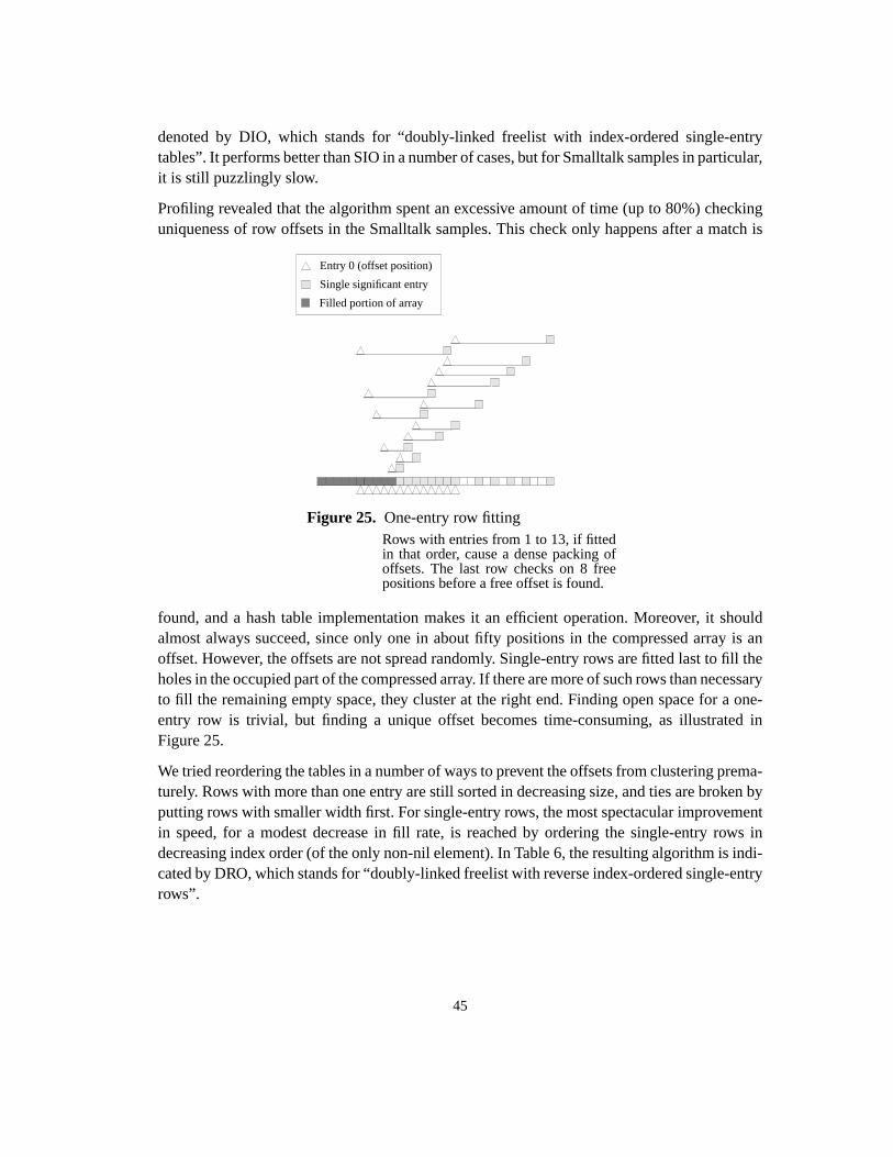
45

denoted by DIO, which stands for “doubly-linked freelist with index-ordered single-entrytables”. It performs better than SIO in a number of cases, but for Smalltalk samples in particular,it is still puzzlingly slow.

Profiling revealed that the algorithm spent an excessive amount of time (up to 80%) checkinguniqueness of row offsets in the Smalltalk samples. This check only happens after a match is

found, and a hash table implementation makes it an efficient operation. Moreover, it shouldalmost always succeed, since only one in about fifty positions in the compressed array is anoffset. However, the offsets are not spread randomly. Single-entry rows are fitted last to fill theholes in the occupied part of the compressed array. If there are more of such rows than necessaryto fill the remaining empty space, they cluster at the right end. Finding open space for a one-entry row is trivial, but finding a unique offset becomes time-consuming, as illustrated inFigure 25.

We tried reordering the tables in a number of ways to prevent the offsets from clustering prema-turely. Rows with more than one entry are still sorted in decreasing size, and ties are broken byputting rows with smaller width first. For single-entry rows, the most spectacular improvementin speed, for a modest decrease in fill rate, is reached by ordering the single-entry rows indecreasing index order (of the only non-nil element). In Table 6, the resulting algorithm is indi-cated by DRO, which stands for “doubly-linked freelist with reverse index-ordered single-entryrows”.

Figure 25. One-entry row fitting

Entry 0 (offset position)

Single significant entry

Filled portion of array

Rows with entries from 1 to 13, if fittedin that order, cause a dense packing ofoffsets. The last row checks on 8 freepositions before a free offset is found.

46

4.4.2 Compression speed

Table 6 shows the fill rates of the three variants, and timings as the average over 20 runs. Cache

effects caused a variation of less than 3%. We omitted the smaller samples because the time wastoo small to be reliably measured.

For all but the C++ and LOV samples, the fill rate is largely independent of the particular algo-rithm used. Fill rates vary slightly because the ordering of single-entry tables trades memory forspeed. The difference between single and doubly-linked freelists, which is most pronounced inthe Geode sample, is caused by the different order in which offsets are checked. SIO puts a rowin the first place that fits, starting from the left edge of the compressed array. DIO and DRO alsogo from left to right, but start with the freelist with the smallest block size. There may be largerblocks to the left of a smaller block, causing a table to be fitted further to the right than strictlynecessary.

The fastest algorithm in almost all cases is DRO. For samples from the same programming envi-ronment, there seems to be a linear relation between the number of classes and the time neededto compress the tables. For SIO, the relation appears quadratic (i.e., twice as many classes takefour times as long).

Absolute performance is excellent, especially compared to previous techniques. For example,the Object sample takes 0.4 seconds to compress (on a SPARCstation-20) compared to thefastest class-based row displacement algorithm in [40] which took 36 minutes on a Mac IIfx.

Fill rate (in %) Timing (in seconds)

System Library C S M SIO DIO DRO SIO DIO DRO

Parcplace Object w/o metaclasses383 4,026 61,775 99.5 99.5 99.4 0.3 0.9 0.2

Smalltalk Object (Parcplace1) 774 5,086 178,230 99.7 99.7 99.6 1.7 4.3 0.4

Parcplace2 1,956 13,474 608,456 99.7 99.7 99.7 14.6 25.3 2.1

Digitalk Digitalk2 534 4,482 154,585 99.7 99.7 99.6 0.8 3.3 0.7

Smalltalk Digitalk3 1,356 10,051 613,654 99.8 99.8 99.8 5.9 13.5 1.6

IBM Smalltalk 2,320 14,009 485,321 99.8 99.8 99.5 32.3 11.4 5.2

Smalltalk VisualAge2 3,241 17,342 1,045,333 99.7 99.7 99.7 167.3 13.6 12.0

Objective-C NextStep 310 2,707 71,334 99.7 99.7 99.6 0.5 2.1 0.2

SELF Self System 4.0 1,801 10,103 1,038,514 99.8 99.8 99.8 9.4 2.4 2.5

C++ ET++ 370 628 14,816 98.5 98.4 97.6 0.04 0.05 0.04

Unidraw/Interviews 613 1,146 13,387 97.6 95.8 95.7 0.2 0.1 0.05

LOV Lov+ObjectEditor 436 2,901 36,052 95.8 91.1 91.1 0.8 0.3 0.2

Geode 1,318 6,555 302,717 74.9 70.8 70.8 49.0 9.6 9.0

Table 6. Compression speed (in seconds, on a 60Mhz SPARCstation-20)C: number of classesS: number of selectorsM: total of legitimate class-selector combinations

SIO: singly-linked freelist with index-ordered single-entry rowsDIO: doubly-linked freelist with index-ordered single-entry rows

DRO: doubly-linked freelist with reverse index-ordered single-entry rows

47

For Object, selector coloring on a Sun-3/80 took about 80 minutes to build the conflict graphand 12 minutes to color it [9]. These timings are measured on different hardware and withdifferent compilers, so that they cannot really be compared directly. However, we believe it issafe to say that on equivalent hardware, selector-based row displacement compressionconstructs dispatch tables at least an order of magnitude faster than these previous techniques.Furthermore, the data shows that row displacement compression is now a practical technique.Though compression may still take too long for an interactive environment, it can be postponed,as outlined in the next section.

4.5 Applicability to interactive programming environments

In an ideal interactive programming environment any change to a program is reflected withoutnoticeable delay. Subsecond response time is required to optimize programmer productivity. Asdiscussed above, both selector coloring and row displacement compression are not fast enoughto hide global refitting of dispatch tables from the user.

Selector-based tables improve on class-based tables, since a global reorganization is only neces-sary when a new class is defined, because this adds a column to the two-dimensional table andthus affects all rows. The definition of a new message just adds a row. Presuming that thecompressed array has space for it, this does not affect the other rows. For class-based tables, thesituation is similar but reversed: defining a new message can affect all rows and cause reorga-nization. Since new messages are defined more often than new classes, selector-based rowdisplacement is better tuned to a development environment.

Still, when it occurs, global reorganization can be painful. As outlined in [39], global refittingcan be postponed until there is time and opportunity, by having a second-stage table that issearched when the main table would deliver a “message not understood” error. For selector-based tables, this second table holds the newly defined classes. Message sends to instances ofnew classes are slower than normal, until the classes are incorporated in the main table.

Thus selector-based row displacement tables can be employed in an interactive programmingenvironment, if the table fitting costs are postponed by using a second-stage table, and at thecost of slower dispatch for recently defined classes.

4.6 Summary

Selector-based row displacement makes table-based message dispatching practical for dynam-ically-typed languages, due to the following two properties:

• Compact dispatch tables. For large single-inheritance class libraries, row displacementtables are less than 0.5% larger than virtual function tables. If multiple inheritance is usedextensively, row displacement outperforms virtual function tables by a factor of two on thetested samples.

48

• Fast dispatch table construction. On a 1995 midrange workstation, compression takes lessthan 2.5 seconds for most of the large class libraries measured. This performance makes thetechnique practical even for interactive programming environments, especially if a second-stage dispatch table is used to postpone global reorganization.

Thus, row displacement dispatch tables provide the dispatch efficiency of virtual functiontables, with comparable memory cost and low compile time overhead, for dynamically-typedobject-oriented programming languages.

For multiple inheritance languages, row displacement performs better than virtual functiontables by more than a factor two (in remaining overhead)

49

5 Analysis of dispatch sequences on modernprocessor architectures

“Fallacy: increasing the depth of pipeliningalways increases performance.”

Hennessy and Patterson [65]

Dispatch cost is intimately coupled with processor implementation. The same dispatchsequence may have different cost on different processor implementations, even if all of themimplement the same architecture (e.g., the SPARC instruction set). In particular, processor pipe-lining and superscalar execution make it impossible to use the number of instructions in a codesequence as an accurate performance indicator. This section characterizes the run-time perfor-mance of dispatch mechanisms on modern pipelined processors by determining the perfor-mance impact of branch latency and superscalar instruction issue. We do this by analyzing callcode sequences, optimally scheduled for the given instruction issue. In addition to providingspecific numbers for three example architectures, our analysis allows bounds on dispatchperformance to be computed for a wide range of possible (future) processors. With the rapidchange in processor design, it is desirable to characterize performance in a way that makes thedependence on certain processor characteristics explicit, so that performance on a newprocessor can be estimated accurately as long as the processor’s characteristics are known.

5.1 Parameters influencing performance

To evaluate the performance of the dispatch mechanisms, we implemented the dispatch instruc-tion sequence of each technique on a simple RISC-like architecture.1 Then, we calculated thecost of the dispatch sequences for three hypothetical processor implementations. P92 representsa scalar implementation as it was typical of processor designs in 1992. P95 is a superscalarimplementation that can execute up to two integer instructions concurrently, representative ofcurrent state-of-the art processor designs. Finally, P97 is an estimate of a 1997 superscalarprocessor with four-instruction issue width and a deeper pipeline. Table 7 lists the detailedprocessor characteristics relevant to the study.

In essence, these processors are abstractions of current commercial processors that have beenreduced to their most important performance features, namely

• Superscalar architecture. The processor can execute several instructions in parallel as longas they are independent. Since access paths to the cache are expensive, all but P97 canexecute at most one load or store per cycle.

1 Assuming a RISC architecture simplifies the discussion, but our results are not restricted to RISC architectures since pipelinedCISC machines have similar performance characteristics. For example, the Intel Pentium processor closely resembles P95.

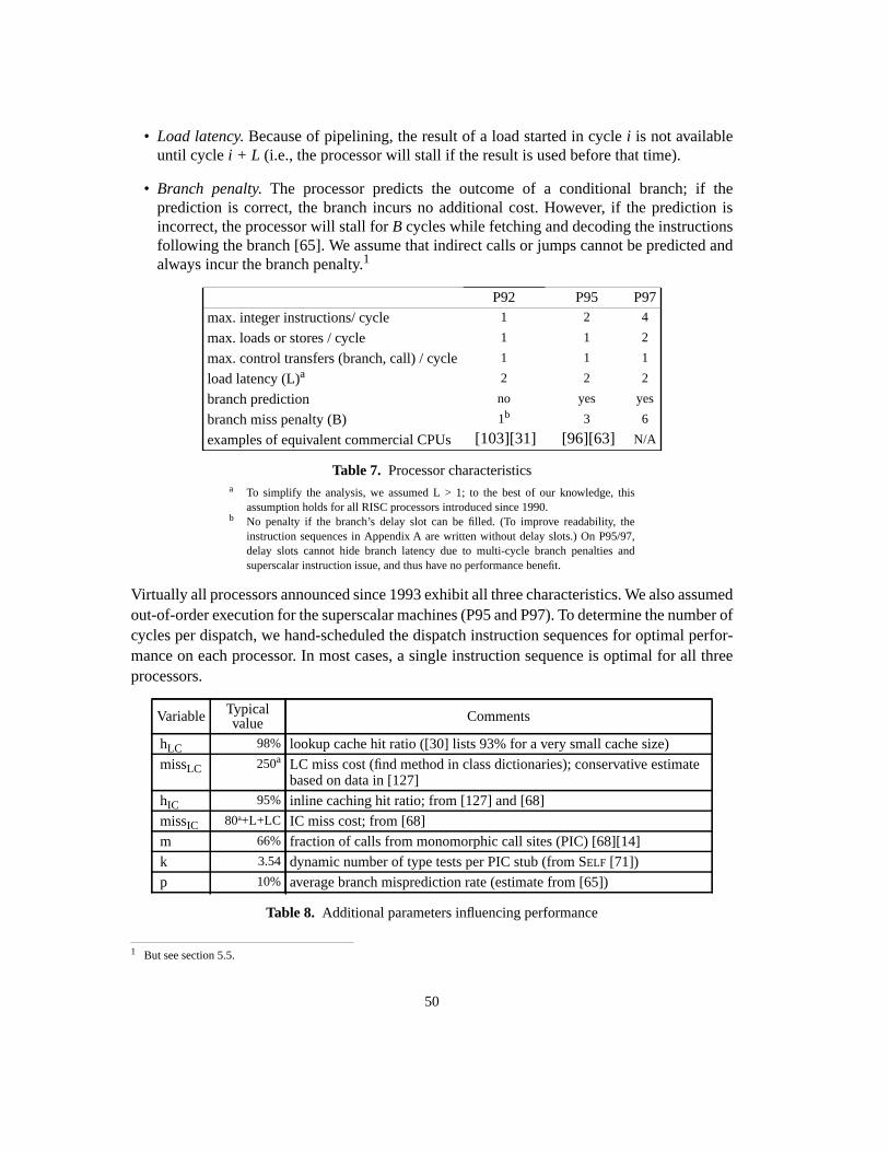
50

• Load latency. Because of pipelining, the result of a load started in cyclei is not availableuntil cyclei + L (i.e., the processor will stall if the result is used before that time).

• Branch penalty. The processor predicts the outcome of a conditional branch; if theprediction is correct, the branch incurs no additional cost. However, if the prediction isincorrect, the processor will stall forB cycles while fetching and decoding the instructionsfollowing the branch [65]. We assume that indirect calls or jumps cannot be predicted andalways incur the branch penalty.1

Virtually all processors announced since 1993 exhibit all three characteristics. We also assumedout-of-order execution for the superscalar machines (P95 and P97). To determine the number ofcycles per dispatch, we hand-scheduled the dispatch instruction sequences for optimal perfor-mance on each processor. In most cases, a single instruction sequence is optimal for all threeprocessors.

a To simplify the analysis, we assumed L > 1; to the best of our knowledge, thisassumption holds for all RISC processors introduced since 1990.

b No penalty if the branch’s delay slot can be filled. (To improve readability, theinstruction sequences in Appendix A are written without delay slots.) On P95/97,delay slots cannot hide branch latency due to multi-cycle branch penalties andsuperscalar instruction issue, and thus have no performance benefit.

1 But see section 5.5.

P92 P95 P97

max. integer instructions/ cycle 1 2 4

max. loads or stores / cycle 1 1 2

max. control transfers (branch, call) / cycle 1 1 1

load latency (L)a 2 2 2

branch prediction no yes yes

branch miss penalty (B) 1b 3 6

examples of equivalent commercial CPUs[103][31] [96][63] N/A

Table 7. Processor characteristics

Variable Typicalvalue Comments

hLC 98% lookup cache hit ratio ([30] lists 93% for a very small cache size)

missLC 250a LC miss cost (find method in class dictionaries); conservative estimatebased on data in [127]

hIC 95% inline caching hit ratio; from [127] and [68]

missIC 80a+L+LC IC miss cost; from [68]

m 66% fraction of calls from monomorphic call sites (PIC) [68][14]

k 3.54 dynamic number of type tests per PIC stub (from SELF [71])

p 10% average branch misprediction rate (estimate from [65])

Table 8. Additional parameters influencing performance

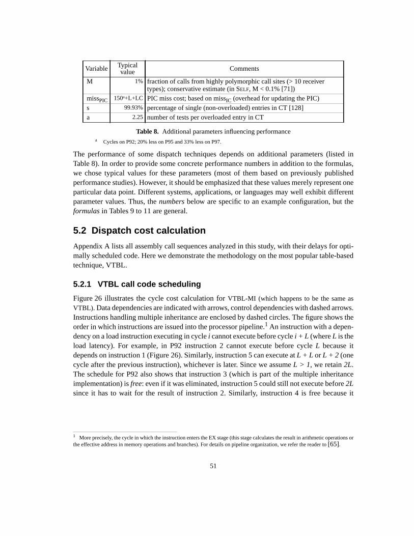
51

The performance of some dispatch techniques depends on additional parameters (listed inTable 8). In order to provide some concrete performance numbers in addition to the formulas,we chose typical values for these parameters (most of them based on previously publishedperformance studies). However, it should be emphasized that these values merely represent oneparticular data point. Different systems, applications, or languages may well exhibit differentparameter values. Thus, thenumbers below are specific to an example configuration, but theformulas in Tables 9 to 11 are general.

5.2 Dispatch cost calculation

Appendix A lists all assembly call sequences analyzed in this study, with their delays for opti-mally scheduled code. Here we demonstrate the methodology on the most popular table-basedtechnique, VTBL.

5.2.1 VTBL call code scheduling

Figure 26 illustrates the cycle cost calculation forVTBL-MI (which happens to be the same as

VTBL). Data dependencies are indicated with arrows, control dependencies with dashed arrows.Instructions handling multiple inheritance are enclosed by dashed circles. The figure shows theorder in which instructions are issued into the processor pipeline.1 An instruction with a depen-dency on a load instruction executing in cyclei cannot execute before cyclei + L (whereL is theload latency). For example, in P92 instruction 2 cannot execute before cycleL because itdepends on instruction 1 (Figure 26). Similarly, instruction 5 can execute atL + L orL + 2 (onecycle after the previous instruction), whichever is later. Since we assumeL > 1, we retain2L.The schedule for P92 also shows that instruction 3 (which is part of the multiple inheritanceimplementation) isfree: even if it was eliminated, instruction 5 could still not execute before2Lsince it has to wait for the result of instruction 2. Similarly, instruction 4 is free because it

a Cycles on P92; 20% less on P95 and 33% less on P97.

1 More precisely, the cycle in which the instruction enters the EX stage (this stage calculates the result in arithmetic operations orthe effective address in memory operations and branches). For details on pipeline organization, we refer the reader to[65].

M 1% fraction of calls from highly polymorphic call sites (> 10 receivertypes); conservative estimate (in SELF, M < 0.1% [71])

missPIC 150a+L+LC PIC miss cost; based on missIC (overhead for updating the PIC)

s 99.93% percentage of single (non-overloaded) entries in CT [128]

a 2.25 number of tests per overloaded entry in CT

Variable Typicalvalue Comments

Table 8. Additional parameters influencing performance

52

executes in the delay slot of the call (instruction 5).1 As a result, VTBL incurs no overhead formultiple inheritance: both versions of the code execute in2L + 2 cycles (see Table 9).

P95 (middle part of Figure 26) can execute two instructions per cycle (but only one of them canbe a memory instruction, see Table 7). Unfortunately, this capability doesn’t benefit VTBLmuch since its schedule is dominated by load latencies and the branch latencyB. Since VTBLuses an indirect call, the processor does not know its target address until after the branchexecutes (in cycle2L). At that point, it starts fetching new instructions, but it takesB cycles untilthe first new instruction reaches the EX (execute) stage of the pipeline [65], resulting in a totalexecution time of2L+B+1. Finally, P97 can execute up to 4 instructions per cycle, but againthis capability is largely unused, except that instructions 2 and 3 (two loads) can execute inparallel. However, the final cycle count is unaffected by this change.

5.2.2 Other techniques

Table A-2 to 8 in Appendix A list call code sequences in assembly for all dispatch techniques,and corresponding optimal code schedules on P92 and P97. We used these schedules to derivethe formulas in Tables 9 to 11: we express dispatch cost as a function of processor parameters(L and B) and algorithmic parameters such as miss ratios, etc. Table 12 contains the rawdispatch times in cycles.

1 Recall that P92 machines had a branch latency B = 1, which can be eliminated using explicit branch delay slots; see[65] fordetails. Since we use a fixed branch penalty for P92, B does not appear as a parameter in Table 4.

1: load [object + #tableOffset], table2: load [table + #selectorOffset], method3: load [table + #deltaOffset], delta4: add object, delta, object5: call method6: <first instruction of target>

1

3

2

4

5

1

3

2

4 5

1

32

45

P92 P95 P97

0

L

L+1

2L

2L+1

2L+2

0

L

L+1

2L+1/2L

2L+1+B

0

L

2L

2L+1+B

6

6

(delay slot)

Figure 26. VTBL-MI schedules and dependencies, cycle counts and assembly code.

6

53

Figure 27a shows the execution time (in processor cycles) of all dispatch implementations onthe three processor models, assuming static typing and single inheritance. Not surprisingly, alltechniques improve significantly upon lookup caching (LC) since LC has to compute a hashfunction during dispatch. The performance of the other dispatch mechanisms is fairly similar,especially on P95 which models current hardware. VTBL and SC are identical for all proces-sors; RD and VTBL are very close for all but the P92 processor. Among these techniques, noclear winner emerges since their relative ranking depends on the processor implementation. Forexample, on P92 VTBL performs better than IC, whereas on P97 IC is better. (Section 5.4 will

static typing dynamic typing

LC hLC*(9+max(7,2L))+(1-hLC)*missLC

VTBL 2+2L N/A

VTBL-MI 2+2L N/A

SC 2+2L 4+2L

RD 3+L + max(L, 3) 7+L+max(3,L)

CT s*(2+3L)+(1-s) *(3+3L+7a) s*(8+3L)+(1-s) *(3+3L+7a)

IC hIC * (2+max(3,L)) + (1-hIC) * missICPIC m * (2+max(3,L)) + (1-m) * (2+L+2k) + M * missPIC

Table 9. P92

static typing dynamic typing

LC hLC * (7+2L+B) +(1-hLC) * missLC

VTBL 1+2L+B N/A

VTBL-MI 1+2L+B N/A

SC 1+2L+B 3+2L+B

RD 1+2L+B 3+2L+B

CT s*(1+3L+B)+(1-s)* (2+3L+B+a(4 +pB)) s*(5+3L+B)+(1-s)* (2+3L+B+a(4 +pB))

IC hIC * (1+L) + (1-hIC) * missICPIC m * (1+L)+(1-m)*(2+L+k(1 +pB)) + M * missPIC

Table 10. P95

static typing dynamic typing

LC hLC * (6+2L+B) +(1-hLC) * missLC

VTBL 1+2L+B N/A

VTBL-MI 1+2L+B N/A

SC 1+2L+B 2+2L+B

RD 1+2L+B 3+2L+B

CT s*(1+3L+B)+(1-s)* (2+3L+B+a(3 +pB)) s*(4+3L+B)+(1-s)* (2+3L+B+a(3 +pB))

IC hIC * (1+L) + (1-hIC) * missICPIC m * (1+L) + (1-m) * (1+L+k(1 +pB)) + M * missPIC

Table 11. P97

54

examine processor influence in detail.) For dynamic typing, the picture is qualitatively the same(Figure 27b).

5.3 Cost of dynamic typing and multiple inheritance

A closer look at Tables 9 to 11 and Figure 27 shows that supporting dynamic typing is surpris-ingly cheap for all dispatch methods, especially on superscalar processors like P95 and P97. Inseveral cases (LC, IC, PIC), dynamic typing incurs no overhead at all. For the other techniques,the overhead is still low since the additional instructions can be scheduled to fit in instructionissue slots that would otherwise go unused. Typical overheads are two cycles per dispatch onP95 and one or two cycles on P97. Thus, on superscalar processors dynamic typing does notsignificantly increase dispatch cost.

The cycle cost of supporting hard-coded offsets for multiple inheritance in VTBL-MI is zero.However, recall that we have simplified the discussion of VTBL-MI for C++ by ignoring virtualbase classes. Using virtual base classes can significantly increase dispatch cost in VTBL-MI.For all other techniques, the cost of multiple inheritance appears not as overhead of messagedispatch, but when referencing an instance variable (see section 3.1.2).

Table 12 shows timings as calculated according to the formulas. Since the performance varia-tions between the two scenarios are so small and do not qualitatively change the situation, wewill only discuss the case using static typing and single inheritance. Of course, dynamic typingand multiple inheritance can affect other aspects of dispatch implementation, as discussed insection 3.4 and 3.5.

Figure 27. Performance of dispatch mechanisms (single inheritance)

P92 P95 P970

5

10

15

20

25

cycl

es p

er s

end

RD

LC

VTBL, SC

CT

ICPIC

RD

(a) static typing (b) dynamic typing

P92 P95 P970

5

10

15

20

25

cycl

es p

er s

end

LC

RD

CT

ICPIC

SC

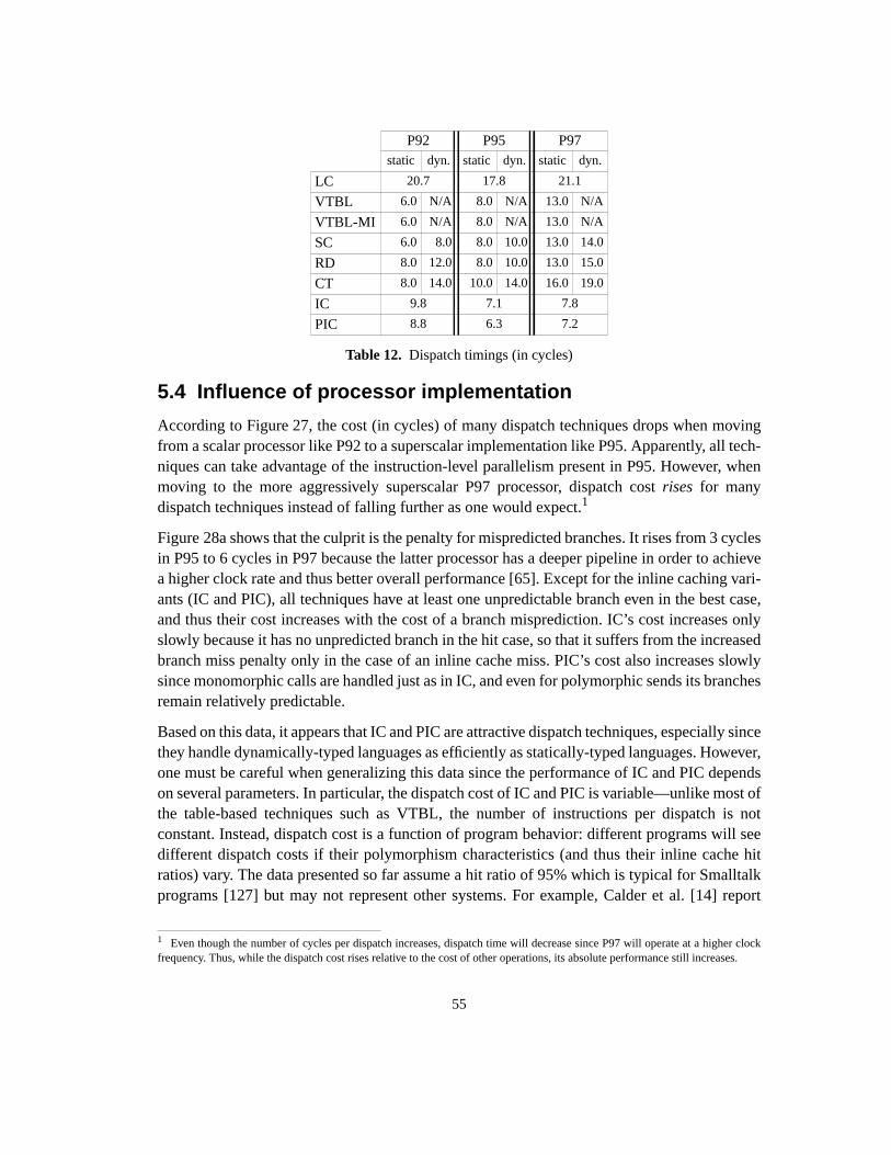
55

5.4 Influence of processor implementation

According to Figure 27, the cost (in cycles) of many dispatch techniques drops when movingfrom a scalar processor like P92 to a superscalar implementation like P95. Apparently, all tech-niques can take advantage of the instruction-level parallelism present in P95. However, whenmoving to the more aggressively superscalar P97 processor, dispatch costrises for manydispatch techniques instead of falling further as one would expect.1

Figure 28a shows that the culprit is the penalty for mispredicted branches. It rises from 3 cyclesin P95 to 6 cycles in P97 because the latter processor has a deeper pipeline in order to achievea higher clock rate and thus better overall performance [65]. Except for the inline caching vari-ants (IC and PIC), all techniques have at least one unpredictable branch even in the best case,and thus their cost increases with the cost of a branch misprediction. IC’s cost increases onlyslowly because it has no unpredicted branch in the hit case, so that it suffers from the increasedbranch miss penalty only in the case of an inline cache miss. PIC’s cost also increases slowlysince monomorphic calls are handled just as in IC, and even for polymorphic sends its branchesremain relatively predictable.

Based on this data, it appears that IC and PIC are attractive dispatch techniques, especially sincethey handle dynamically-typed languages as efficiently as statically-typed languages. However,one must be careful when generalizing this data since the performance of IC and PIC dependson several parameters. In particular, the dispatch cost of IC and PIC is variable—unlike most ofthe table-based techniques such as VTBL, the number of instructions per dispatch is notconstant. Instead, dispatch cost is a function of program behavior: different programs will seedifferent dispatch costs if their polymorphism characteristics (and thus their inline cache hitratios) vary. The data presented so far assume a hit ratio of 95% which is typical for Smalltalkprograms [127] but may not represent other systems. For example, Calder et al. [14] report

1 Even though the number of cycles per dispatch increases, dispatch time will decrease since P97 will operate at a higher clockfrequency. Thus, while the dispatch cost rises relative to the cost of other operations, its absolute performance still increases.

P92 P95 P97static dyn. static dyn. static dyn.

LC 20.7 17.8 21.1

VTBL 6.0 N/A 8.0 N/A 13.0 N/A

VTBL-MI 6.0 N/A 8.0 N/A 13.0 N/A

SC 6.0 8.0 8.0 10.0 13.0 14.0

RD 8.0 12.0 8.0 10.0 13.0 15.0

CT 8.0 14.0 10.0 14.0 16.0 19.0

IC 9.8 7.1 7.8

PIC 8.8 6.3 7.2

Table 12. Dispatch timings (in cycles)

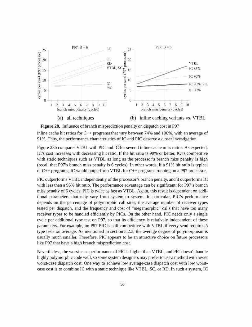
56

inline cache hit ratios for C++ programs that vary between 74% and 100%, with an average of91%. Thus, the performance characteristics of IC and PIC deserve a closer investigation.

Figure 28b compares VTBL with PIC and IC for several inline cache miss ratios. As expected,IC’s cost increases with decreasing hit ratio. If the hit ratio is 90% or better, IC is competitivewith static techniques such as VTBL as long as the processor’s branch miss penalty is high(recall that P97’s branch miss penalty is 6 cycles). In other words, if a 91% hit ratio is typicalof C++ programs, IC would outperform VTBL for C++ programs running on a P97 processor.

PIC outperforms VTBL independently of the processor’s branch penalty, and it outperforms ICwith less than a 95% hit ratio. The performance advantage can be significant: for P97’s branchmiss penalty of 6 cycles, PIC is twice as fast as VTBL. Again, this result is dependent on addi-tional parameters that may vary from system to system. In particular, PIC’s performancedepends on the percentage of polymorphic call sites, the average number of receiver typestested per dispatch, and the frequency and cost of “megamorphic” calls that have too manyreceiver types to be handled efficiently by PICs. On the other hand, PIC needs only a singlecycle per additional type test on P97, so that its efficiency is relatively independent of theseparameters. For example, on P97 PIC is still competitive with VTBL if every send requires 5type tests on average. As mentioned in section 3.2.3, the average degree of polymorphism isusually much smaller. Therefore, PIC appears to be an attractive choice on future processorslike P97 that have a high branch misprediction cost.

Nevertheless, the worst-case performance of PIC is higher than VTBL, and PIC doesn’t handlehighly polymorphic code well, so some system designers may prefer to use a method with lowerworst-case dispatch cost. One way to achieve low average-case dispatch cost with low worst-case cost is to combine IC with a static technique like VTBL, SC, or RD. In such a system, IC

1 2 3 4 5 6 7 8 9 100

5

10

15

20

25

cycl

es p

er s

end

(P97

pro

cess

or)

branch miss penalty (cycles)

P97: B = 6

PICIC

VTBL, SC

CT

LC

RD

Figure 28. Influence of branch misprediction penalty on dispatch cost in P97

1 2 3 4 5 6 7 8 9 100

5

10

15

20

25

cycl

es p

er s

end

(P97

pro

cess

or)

branch miss penalty (cycles)

P97: B = 6

VTBL

IC 95%, PIC

IC 98%

IC 85%

IC 90%

(a) all techniques (b) inline caching variants vs. VTBL

57

would handle monomorphic call sites, and the static technique would handle polymorphic sites.(Another variant would add PIC for moderately polymorphic call sites.) The combination’s effi-ciency depends on the percentage of call sites that are handled well by IC. Obviously, call siteswith only one target fall in this category but so do call sites whose target changes very infre-quently (so that the rare IC miss doesn’t have a significant performance impact). The scheme’sdispatch cost is a linear combination of the two techniques’ cost. For example, Calder’s data[14] suggest that at least 66% of all virtual calls in C++ could be handled without misses by IC,reducing dispatch cost on P97 from 13 cycles for a pure VTBL implementation to 13* 0.34 + 4* 0.66 = 5.6 cycles for VTBL+IC. In reality, the performance gain might be even higher sincecalls from call sites incurring very few misses could also be handled by IC. Even though thisdata is by no means conclusive, the potential gain in dispatch performance suggests that imple-mentors should include such hybrid dispatch schemes in their list of dispatch mechanisms toevaluate.

5.5 Limitations

The above analysis leaves a number of issues unexplored. Three issues are particularly impor-tant: cache behavior, application code surrounding the dispatch sequence, and hardware predic-tion of indirect branches.

We do not consider memory hierarchy effects (cache misses); all results assume that memoryreferences will always hit the first level memory cache. If all dispatch techniques have similarlocality of reference, this assumption should not distort the results. However, without thoroughbenchmarking it remains unsubstantiated.

Application instructions surrounding the dispatch sequence (e.g., instructions for parameterpassing) can be scheduled to fit in the “holes” of the dispatch code, lowering the overall execu-tion time, and thus effectively lowering dispatch overhead. Therefore, measuring dispatch costin isolation (as done in this study) may overestimate the true cost of dispatch techniques. Unfor-tunately, the effect of co-scheduling application code with dispatch code depends on the natureof the application code and thus is hard to determine. Furthermore, the average basic blocklength (and thus the number of instructions readily available to be scheduled with the call) isquite small, usually between five and six [65]. On superscalar processors (especially on P97)most dispatch sequences have plenty of “holes” to accommodate that number of instructions.Thus, we assume that most techniques would benefit from co-scheduled application code toroughly the same extent. In Section 6 we will study two variants of VTBL in order to determinethe effect of co-scheduling.

A branch target buffer (BTB) [65] allows hardware to predict indirect calls by storing the targetaddress of the previous call, similar to inline caching. The study in this section assumes thatprocessors do not use BTBs. Therefore, the formula’s for table-based techniques calculate abound on the cost of message dispatch (ignoring memory effects). This worst case cost demon-strates the importance of accurate indirect branch prediction in hardware. BTBs are relatively

58

expensive (since they have to store the full target address, not just a few prediction bits).However, future processors are likely to incorporate BTBs since they will have enough transis-tors available to accommodate a reasonably-sized BTB, and because indirect calls can occurfrequently in procedural programs as well1 (see Section 7). Some processors (most notably,Intel’s Pentium processor and its successor P6) have small BTBs today. Interestingly, BTBsbehave similar to inline caches—they work well for monomorphic call sites but badly for highlypolymorphic call sites. For example, the performance of VTBL on such a processor would besimilar to the VTBL+IC scheme discussed above. The impact of BTBs on dispatch performancecan be estimated by reducing the value of branch penalty B in the formulas of Tables 10 and 11,but the extent of the reduction depends on the BTB miss ratio (i.e., inline cache miss ratio) ofthe application. We also explore this effect in Section 6.

5.6 Summary

We have evaluated the dispatch cost of a range of dispatch mechanisms, taking into account theperformance characteristics of modern pipelined superscalar microprocessors. On such proces-sors, objectively evaluating performance is difficult since the cost of each instruction dependson surrounding instructions and the cost of branches depends on dynamic branch prediction. Inparticular, some instructions may be “free” because they can be executed in parallel with otherinstructions, and unpredictable conditional branches as well as indirect branches are expensive(and likely to become more expensive in the future). On superscalar architectures, countinginstructions to estimate performance is highly misleading. We have studied dispatch perfor-mance on three processor models designed to represent the past (1992), present (1995), andfuture (1997) state of the art in processor implementation.

We have analyzed the run-time performance of dispatch mechanisms as a function of processorcharacteristics such as branch latency and superscalar instruction issue, and as a function ofsystem parameters such as the average degree of polymorphism in application code. Theresulting formulas allow dispatch performance to be computed for a wide range of possible(future) processors and systems. In addition, we also present formulas for computing the spacecost of the various dispatch techniques. Our study has produced several results:

• The relative performance of dispatch mechanisms varies with processor implementation.Whereas some mechanisms become relatively more expensive (in terms of cycles perdispatch) on more aggressively superscalar processors, others become less expensive. Nosingle dispatch mechanism performs best on all three processor models.

• Mechanisms employing indirect branches (i.e., all table-based techniques) may not performwell on current and future hardware since indirect branches incur multi-cycle pipelinestalls, unless some form of indirect branch prediction is present. Inline caching variants

1 Procedure returns occur frequently even in non-polymorphic programs, but these can be handled more efficiently by a returnaddress prediction buffer[63].

59

pipeline very well and do not incur such stalls. On deeply pipelined superscalar processorslike the P97, inline caching techniques may substantially outperform even the most efficienttable-based techniques.

• Hybrid techniques combining inline caching with a table-based method may offer bothexcellent average dispatch cost as well as a low worst-case dispatch cost.

• On superscalar processors, the additional cost of supporting dynamic typing is small (oftenzero) because the few additional instructions usually fit into otherwise unused instructionissue slots.

Even though selecting the best dispatch mechanism for a particular system is still difficult sinceit involves many factors, the data presented here should allow dispatch cost bounds to be esti-mated for a wide range of systems. Therefore, we hope that this study will be helpful to systemimplementors who need to choose the dispatch mechanism best suited to their needs.

60

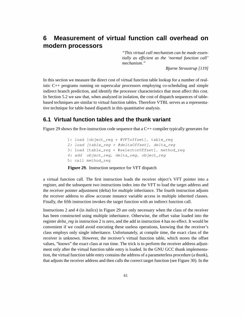
61

6 Measurement of virtual function call overhead onmodern processors

“This virtual call mechanism can be made essen-tially as efficient as the ‘normal function call’mechanism.”

Bjarne Stroustrup [119]

In this section we measure the direct cost of virtual function table lookup for a number of real-istic C++ programs running on superscalar processors employing co-scheduling and simpleindirect branch prediction, and identify the processor characteristics that most affect this cost.In Section 5.2 we saw that, when analyzed in isolation, the cost of dispatch sequences of table-based techniques are similar to virtual function tables. Therefore VTBL serves as a representa-tive technique for table-based dispatch in this quantitative analysis.

6.1 Virtual function tables and the thunk variant

Figure 29 shows the five-instruction code sequence that a C++ compiler typically generates for

a virtual function call. The first instruction loads the receiver object’s VFT pointer into aregister, and the subsequent two instructions index into the VFT to load the target address andthe receiver pointer adjustment (delta) for multiple inheritance. The fourth instruction adjuststhe receiver address to allow accurate instance variable access in multiple inherited classes.Finally, the fifth instruction invokes the target function with an indirect function call.

Instructions 2 and 4 (initalics) in Figure 29 are only necessary when the class of the receiverhas been constructed using multiple inheritance. Otherwise, the offset value loaded into theregisterdelta_reg in instruction 2 is zero, and the add in instruction 4 has no effect. It would beconvenient if we could avoid executing these useless operations, knowing that the receiver’sclass employs only single inheritance. Unfortunately, at compile time, the exact class of thereceiver is unknown. However, the receiver’s virtual function table, which stores the offsetvalues, “knows” the exact class at run time. The trick is to perform the receiver address adjust-ment only after the virtual function table entry is loaded. In the GNU GCC thunk implementa-tion, the virtual function table entry contains the address of a parameterless procedure (a thunk),that adjusts the receiver address and then calls the correct target function (see Figure 30). In the

Figure 29. Instruction sequence for VFT dispatch

1: load [object_reg + #VFToffset], table_reg2: load [table_reg + #deltaOffset], delta_reg3: load [table_reg + #selectorOffset], method_reg4: add object_reg, delta_reg, object_reg5: call method_reg

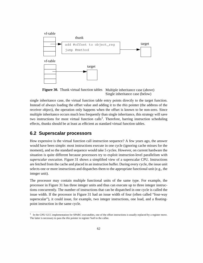
62

single inheritance case, the virtual function table entry points directly to the target function.Instead of always loading the offset value and adding it to thethis pointer (the address of thereceiver object), the operation only happens when the offset is known to be non-zero. Sincemultiple inheritance occurs much less frequently than single inheritance, this strategy will savetwo instructions for most virtual function calls1. Therefore, barring instruction schedulingeffects, thunks should be at least as efficient as standard virtual function tables.

6.2 Superscalar processors

How expensive is the virtual function call instruction sequence? A few years ago, the answerwould have been simple: most instructions execute in one cycle (ignoring cache misses for themoment), and so the standard sequence would take 5 cycles. However, on current hardware thesituation is quite different because processors try to exploit instruction-level parallelism withsuperscalar execution. Figure 31 shows a simplified view of a superscalar CPU. Instructionsare fetched from the cache and placed in an instruction buffer. During every cycle, the issue unitselects one or more instructions and dispatches them to the appropriate functional unit (e.g., theinteger unit).

The processor may contain multiple functional units of the same type. For example, theprocessor in Figure 31 has three integer units and thus can execute up to three integer instruc-tions concurrently. The number of instructions that can be dispatched in one cycle is called theissue width. If the processor in Figure 31 had an issue width of four (often called “four-waysuperscalar”), it could issue, for example, two integer instructions, one load, and a floating-point instruction in the same cycle.

1 In the GNU GCC implementation for SPARC executables, one of the offset instructions is usually replaced by a register move.The latter is necessary to pass thethis pointer in register %o0 to the callee.

add #offset to object_reg

jump #method

target

Figure 30. Thunk virtual function tables

target

thunkvf-table

vf-table

Multiple inheritance case (above)Single inheritance case (below)

63

Of course, there is a catch: two instructions can only execute concurrently if they are indepen-dent. There are two kinds of dependencies: data dependencies and control dependencies.Datadependencies arise when the operands of an instruction are the results of previous instructions;in this case, the instruction cannot begin to execute before all of its inputs become available. Forexample, instructions 2 and 3 of the VFT dispatch sequence can execute concurrently since theyare independent, but neither of them can execute concurrently with instruction 1 since they bothuse the VFT pointer loaded in instruction 1.

The second form of dependencies,control dependencies, result from the fact that some instruc-tions influence the flow of control. For example, the instructions following a conditional branchare not known until the branch executes and determines the next instruction to execute (i.e.,whether the branch is taken or not). Therefore, even if an instruction after the branch has no datadependencies, it cannot be executed concurrently with (or before) the branch itself.

Both forms of dependencies may carry an execution time penalty because of pipelining.Whereas the result of arithmetic instructions usually is available in the next cycle (for a latencyof one cycle), the result of a load issued in cyclei is not available until cyclei+2 or i+3 (for aload latency L of 2 or 3 cycles) on most current processors even in the case of a first-level cachehit. Thus, instructions depending on the loaded value cannot begin execution until L cycles afterthe load. Similarly, processors impose abranch penalty of B cycles after conditional or indirectbranches: when a branch executes in cyclei (so that the branch target address becomes known),it takes B cycles to refill the processor pipeline until the first instruction after the branch reachesthe execute stage of the pipeline and produces a result.

To summarize, on ideal hardware (with infinite caches and an infinite issue width), the data andcontrol dependencies between instructions impose a lower limit on execution time1. If Ninstructions were all independent, they could execute in a single cycle, but if each of themdepended on the previous one they would take at least N cycles to execute. Thus, the number of

1 A new technique,value prediction [93], which is currently still in a research stage, can remove this limit. A correct predictionallows the instruction that uses a value to execute before the instruction that produces the value, thus bypassing data-dependencies.

load/store unit

instruction buffer

issue unit

branch unitinteger unit FPU

Figure 31. Simplified organization of a superscalar CPU

64

instructions becomes only an approximate predictor of execution time on superscalar proces-sors. Even though actual processors do not have infinite resources, this effect still is significantas we shall see later in this paper.

In a previous study Section 5.2 we approximated the dispatch cost of several techniques byanalyzing the call sequence and describing their cost as a function of load latency and branchpenalty, taking into account superscalar instruction issue. However, this approximation (2L + B+ 1 for VFT dispatch) is only an upper bound on the true cost, and the actual cost might belower. The next few sections explain why.

6.2.1 BTB branch prediction

Since branches are very frequent (typically, every fifth or sixth instruction is a branch [65]) andbranch penalties can be quite high (ranging up to 15 cycles on the Intel Pentium Pro processor[101]), superscalar processors try to reduce the average cost of a branch with branch prediction.Branch prediction hardware guesses the outcome of a branch based on previous executions andimmediately starts fetching instructions from the predicted path. If the prediction is correct, thenext instruction can execute immediately, reducing the branch latency to one cycle; if predictedincorrectly, the processor incurs the full branch penalty B. Predictions are based on previousoutcomes of branches. Typically, the branch’s address is used as an index into a prediction table.For conditional branches, the result is a single bit indicating whether the branch is predictedtaken or not taken, and typical prediction hit ratios exceed 90% [65].

For indirect branches, the prediction mechanism must provide a full target address, not just ataken/not taken bit. Abranch target buffer (BTB) accomplishes this by storing the predictedaddress in a cache indexed by the branch address (very similar to a data cache). When theprocessor fetches an indirect branch, it accesses the BTB using the branch instruction’s address.If the branch is found, the BTB returns its last target address and the CPU starts fetching instruc-tions from that address before the branch is even executed. If the prediction is wrong, or if thebranch wasn’t found, the processor stalls for B cycles and updates the BTB by storing thebranch and its new target address.

BTBs affect the cost of the VFT dispatch sequence: if the virtual call was executed previously,is still cached in the BTB, and invokes the same function as in the previous execution, thebranch penalty is avoided, reducing the sequence’s cost to 2L + 1. We explore more sophisti-cated and accurate branch prediction schemes in Section 7 and beyond.

6.2.2 Advanced superscalar execution

To improve performance, modern processors employ two additional techniques that candecrease the performance impact of dependencies.

First, instructions may be executedout of order: an instructionI that is waiting for its inputs tobecome available does not stall all instructions after it. Instead, those instructions may execute

65

before Iif their inputs are available. Additional hardware ensures that the program semantics arepreserved; for example, if instructions I1 and I2 write the same register, I1 will not overwrite theresult of I2 even if I2 executes first. Out-of-order execution increases throughput by allowingother instructions to proceed while some instructions are stalled.

Second,speculative execution takes this idea one step further by allowing out-of-order execu-tion across conditional or indirect branches. That is, the processor may speculatively executeinstructions before it is known whether they actually should be executed. If speculation failsbecause a branch is mispredicted, the effects of the speculatively executed instructions have tobe undone, again requiring extra hardware. Because branches are so frequent, speculatingacross them can significantly improve performance if branches can be predicted accurately.

Of course, the processor cannot look arbitrarily far ahead in the instruction stream to findinstructions that are ready to execute. For one, the probability of fetching from the correctexecution path decreases exponentially with each predicted branch. Also, the issue units mustselect the next group of instructions to be issued from the buffer within one cycle, thus limitingthe size of that buffer. The most aggressive designs available today select their instructions froma buffer of about 30-40 instructions [100][101], so that instructions have to be reasonably“near” the current execution point in order to be issued out-of-order.

6.2.3 Co-scheduling of application code

With speculative, out-of-order execution the cost of the VFT dispatch sequence is not onlyhighly variable (depending on the success of branch prediction), but it cannot be computed inisolation from its surrounding code. For example, if many other instructions precede thedispatch sequence, they could execute during the cycles where the processor would otherwiselay idle waiting for the loads to complete. Or vice versa, the dispatch instructions could fit intoempty issue slots of the rest of the basic block. This co-scheduling of the application anddispatch code may reduce the overall cost significantly, possibly to the point where completelyremoving the dispatch code would not speed up the program at all (since all dispatch instruc-tions fit into otherwise empty issue slots). Thus, at least in theory, a dispatch implementationmay reach zero overhead (i.e., add no cycles to the execution time) even though it does intro-duce extra instructions.

6.2.4 Summary

While all of the processor features discussed above improve performance on average, they alsoincrease the variability of an instruction’s cost since it depends not only on the instruction itself(or the instruction and its inputs), but also on the surrounding code. Most processors sold today(e.g., the Intel Pentium and Pentium Pro processors, as well as virtually all RISC processorsintroduced since 1995) incorporate several or all of these features. As a result, it is hard topredict how expensive the average C++ virtual function call is on a current-generation PC or

66

workstation. The experiments described in the rest of this paper aim to shed some light on thisquestion.

6.3 Method

It is hard to measure virtual function call cost directly since we cannot usually run program Pideal

(the program without any dispatch code). Although it is fairly easy to count the number ofinstructions executed on behalf of dynamic dispatch, this measure does not accurately reflectthe cost in processor cycles. On modern pipelined processors with multiple instruction issue thecost of an instruction may vary greatly. For example, on a 4-way superscalar processor with abranch penalty of 6, an instruction can take anywhere between 0.25 and 7 cycles1.

Therefore we measure the direct cost of virtual function table lookup bysimulating the execu-tion of P and Pideal. Using an executable editor and a superscalar processor simulator, wecompute the execution times of both programs, thus arriving at the direct cost of dispatch. Inaddition to allowing dispatch cost to be measured at all, simulation also facilitates exploring abroad range of possible processor implementations, thus making it possible to anticipate perfor-mance trends on future processors.

6.3.1 Simulation scheme

Figure 32 shows an overview of our experimental approach: first, the C++ program compiled byan optimizing compiler (we used GNU gcc 2.6.3 and 2.7.2 with options -O2 -msupersparc).Then, an application that uses the EEL executable editing library [88] detects the dispatchinstructions and produces a file with their addresses. Using this file as well as a processordescription, the superscalar processor simulator then runs the benchmark.

The simulator executes SPARC programs using theshade tracing tool [29]. Shade alwaysexecutes all instructions of the program so that programs produce the same results as if theywere executed on the native machine. Each instruction executed is then passed to a superscalarprocessor simulator that keeps track of the time that would be consumed by this instruction onthe simulated processor. Optionally, the simulation of dispatch instructions can be suppressed(i.e., they are executed but not passed to the timing simulator), thus simulating the execution ofPideal , the program using the perfect, zero-cost dynamic dispatch scheme.

The cycle-level simulator schedules instructions from a 32-entry instruction window. As soonas an instruction is eligible for execution (the instructions it depends on have been executed andan appropriate functional unit is available), its latency is calculated, taking into account cachingan branch prediction effects. For this purpose we adapted the PowerSim simulator (for thePowerPC ISA) used by Adam Talcott [120], to the SPARC architecture.

1 In the absence of cache misses.

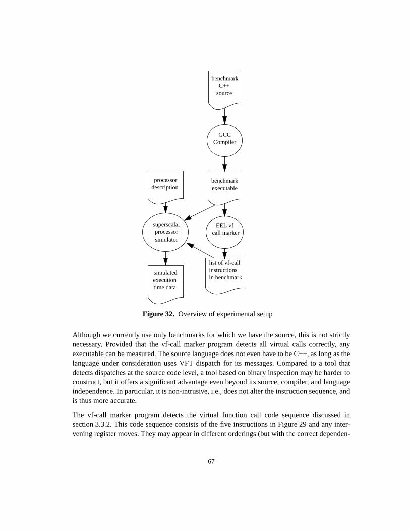
67

Although we currently use only benchmarks for which we have the source, this is not strictlynecessary. Provided that the vf-call marker program detects all virtual calls correctly, anyexecutable can be measured. The source language does not even have to be C++, as long as thelanguage under consideration uses VFT dispatch for its messages. Compared to a tool thatdetects dispatches at the source code level, a tool based on binary inspection may be harder toconstruct, but it offers a significant advantage even beyond its source, compiler, and languageindependence. In particular, it is non-intrusive, i.e., does not alter the instruction sequence, andis thus more accurate.

The vf-call marker program detects the virtual function call code sequence discussed insection 3.3.2. This code sequence consists of the five instructions in Figure 29 and any inter-vening register moves. They may appear in different orderings (but with the correct dependen-

benchmarkC++

source

Figure 32. Overview of experimental setup

GCCCompiler

EEL vf-call marker

list of vf-callinstructionsin benchmark

benchmarkexecutable

processordescription

superscalarprocessorsimulator

simulatedexecutiontime data

68

cies), possibly spread out over different basic blocks. Since the code sequence is highlycharacteristic, the marker program is very accurate, detecting virtual calls exactly for mostprograms.1 For three benchmarks the marker is slightly imprecise, erring by 0.4% or less. Onlyin ixx, 2.3% of the calls went undetected so that our measurements slightly underestimate thedirect dispatch cost for this benchmark.

6.3.2 Benchmarks

We tested a suite of two small and six large C++ applications totalling over 90,000 lines of code(Table 13). In general, we tried to obtain large, realistic applications rather than small, artificialbenchmarks. Two of the benchmarks (deltablue andrichards) are much smaller than the others;they are included for comparison with earlier studies (e.g., [72][62]).Richards is the onlysynthetic benchmark in our suite (i.e., the program was never used to solve any real problem).We did not yet test any programs for which only the executables were available.

For every program exceptporky2 we also tested an “all-virtual” version (indicated by “-av”suffix) which was compiled from a source in which all member functions except operators anddestructors were declared virtual. We chose to include these program versions in order to simu-late programming styles that extensively use abstract base classes defining virtual functionsonly (C++’s way of defining interfaces). For example, the Taligent CommonPoint frameworksprovide all functionality through virtual functions, and thus programs using CommonPoint (orsimilar frameworks) are likely to exhibit much higher virtual function call frequencies. Lackingreal, large, freely available examples of this programming style, we created the “all virtual”programs to provide some indication of the virtual function call overhead of such programs.

1 We cross-checked this by using VPROF, a source-level virtual function profiler for GCC[5].2 Porky cannot be compiled as “all virtual” without a large effort of manual function renaming.

name description lines

deltablue incremental dataflow constraint solver 1,000

eqn type-setting program for mathematical equations 8,300

idl SunSoft’s IDL compiler (version 1.3) using the demonstration back end whichexercises the front end but produces no translated output.

13,900

ixx IDL parser generating C++ stubs, distributed as part of the Fresco library (whichis part of X11R6). Although it performs a function similar to IDL, the programwas developed independently and is structured differently.

11,600

lcom optimizing compiler for a hardware description language developed at the Uni-versity of Guelph

14,100

porky back-end optimizer that is part of the Stanford SUIF compiler system 22,900

richards simple operating system simulator 500

troff GNU groff version 1.09, a batch-style text formatting program 19,200

Table 13. Benchmark programs

69

These versions can also be used to approximate the behavior of programs written in languageswhere (almost) every function is virtual, e.g., Java or Modula-3.

For each benchmark, Table 14 shows the number of executed instructions, the number of virtualfunction calls, and the average number of instructions between calls. All numbers are dynamic,i.e., reflect run-time execution counts unless otherwise mentioned. All programs were simulatedin their entire length as shown in Table 14. Simulation consumed a total of about one CPU-yearof SPARCstation-20 time.

6.3.3 Processors

Table 16 shows an overview of recently introduced processors. Since we could not possiblysimulate all of these processors and their subtle differences, we chose to model a hypotheticalSPARC-based processor that we dubbed P96 because it is meant to resemble the averageprocessor introduced today.

program version instructions virtualcalls

instructions pervirtual call

deltablueoriginal 40,427,339 615,100 65

all-virtual 79,082,867 5,145,581 15

eqnoriginal 97,852,301 100,207 976

all-virtual 108,213,587 1,267,344 85

idloriginal 91,707,462 1,755,156 52

all-virtual 99,531,814 3,925,959 25

ixxoriginal 30,018,790 101,025 297

all-virtual 34,000,249 606,463 56

lcomoriginal 169,749,862 1,098,596 154

all-virtual 175,260,461 2,311,705 75

richardsoriginal 8,119,196 65,790 123

all-virtual 15,506,753 1,146,217 13

trofforiginal 91,877,525 809,312 113

all-virtual 114,607,159 3,323,572 34

porky original 748,914,861 3,806,797 196

Table 14. Basic characteristics of benchmark programs (dynamic counts)

70

For our experiments, we ran all benchmarks on P96 to obtain the base results for the dispatchoverhead. To examine the effects of the most important processor features, we then varied eachparameter while keeping all others constant. Finally, we also measured a few individual config-urations that resemble existing processors (Table 16). P96-noBTB resembles the UltraSPARCin that it lacks a BTB, i.e., does not predict indirect branches. P96-Pro resembles the PentiumPro in its branch configuration, in that it has a high branch penalty. Finally, P2000 is an ideal-ized processor with essentially infinite hardware resources; we use it to illustrate the impact ofthe branch penalty on a processor that has virtually no other limitations on instruction issue.

a BTB = branch target buffer size; BHT = branch history table size (branchhistories are used to predict the direction of conditional branches)

b In the Pentium, BTB and BHT are joined. Each entry in the table stores thebranch target and 16 2-bit counters, one for each possible 4-bit local history

c 16Kx2 means the cache is 16K bytes, and 2-way associative

Processor UltraSPARC

MIPSR10K

DECAlpha21164

PowerPC 604

IntelPentium

Pro

Shipping date 95 95 95 95 95

Size of BTB 0 0 0 64 512

Size of BHTa 2048 512 2048 512 8192b

Branch Penalty 4 4 5 1-3 11-15

Issue Width 4 5 4 4 3

Load Latency 2 2 2 2 3

Primary I-cachec 16Kx2 32Kx2 8Kx1 32Kx4 8K

Primary D-cache 16Kx1 32Kx2 8Kx1 32Kx4 8K

Out-of-order? Y Y Y Y Y

Speculative? Y Y Y Y Y

Table 15. Characteristics of recently introduced processors

Processor P96 P96-noBTB P96-Pro P2000/bp1 P2000/bp10

Size of BTB 256 0 512 1024 1024

Size of BHT 1024 1024 0 1024 1024

Branch Penalty 4 4 15 1 10

Issue Width 4 4 4 32 32

Load Latency 2

Primary I-cache 32K, 2-way associative

Primary D-cache 32K, 2-way associative

Out-of-order? Y

Speculative? Y

Table 16. Characteristics of simulated processors

71

It should be noted that none of these processors is intended to exactly model an existingprocessor; for example, the Intel Pentium Pro’s instruction set and microarchitecture is verydifferent from P96-Pro, and so the latter should not be used to predict the Pentium Pro’s perfor-mance on C++ programs. Instead, we use these processors to mark plausible points in thedesign space, and their distance and relationship to illustrate particular effects or trends.

6.4 Results

This section first examine the cost of dynamic dispatch on the baseline architecture, P96, andthen examines the impact of individual architectural parameters (branch penalty/prediction,load latency, and issue width).

6.4.1 Instructions and cycles

First, we will examine the cost of dynamic dispatch on the baseline architecture, P96. Recallthat we define the cost as the additional cycles spent relative to a “perfect” dispatch implemen-tation that implements each dispatch with a direct call. Figure 33 and Figure 34 show the

results. On the standard benchmarks, the cost varies from 1.4% foreqn to 29% fordeltablue,with a median overhead of 5.2%. For the all-virtual versions, the overhead increases to between4.7% and 47% with a median overhead of 13%. The standard benchmarks spend a median 3.7%of their instructions on dispatch, and the all-virtual versions a median of 13.7%. For the stan-dard benchmarks the cycle cost is larger than the cost in the number of instructions executed; on

Figure 33. Direct cost of standard VFT dispatch (unmodified benchmarks)

eqn

trof

f

ixx

lcom id

l

rich

ards

delta

blue

pork

y

0%

2%

4%

6%

8%

10%

12%

14%

Rel

ativ

e ov

erhe

ad

instructions

cycles

29%

72

average, it is a median 1.7 times larger. This difference confirms that the VFT dispatch sequencedoes not schedule well on a superscalar processor, compared to non-dispatch code. However,this effect varies substantially between benchmarks. The largest difference is found ineqn (2.8times) and deltablue (3.8 times). Since the dispatch sequence is always the same, this indicatesthat the instructions surrounding a call can significantly affect the cost of virtual functionlookup, or that virtual calls are more predictable in some programs than in others. We willexplore these questions shortly.

6.4.2 Thunks

Figure 35 compares the cycle cost of standard and thunk implementations for the unmodifiedbenchmarks1. Thunks have a smaller cycle overhead than regular tables for all benchmarks,using a median of 79% of the cycles of the regular implementation. Figure 36 shows the cyclecost for the all-virtual benchmarks. Here, thunks have 72% of the regular overhead. The exactamount of the gain varies greatly between benchmarks. For example, the thunk overhead forixxanddeltablue is only 15% and 47% of the regular overhead, while fortroff, thunks use almostas many cycles as standard tables (98%).

How can thunks, in some cases, improve dispatch performance by more than a factor of two?One reason for the difference is the unnecessary receiver address adjustment that is avoidedwith thunks (instructions 2 and 4 in Figure 29). In the thunk implementation, instructions that

1 Since GCC cannot compileidl, idl-av, andlcom-av with thunks, these benchmarks are missing from Figure 35 and Figure 36.

eqn-

av

trof

f-av

ixx-

av

lcom

-av

idl-

av

rich

ards

-av

delta

blue

-av

0%

5%

10%

15%

20%

25%

30%

35%

40%

45%

50%R

elat

ive

over

head

instructions

cycles

Figure 34. Direct cost of standard VFT dispatch (all-virtual benchmarks)

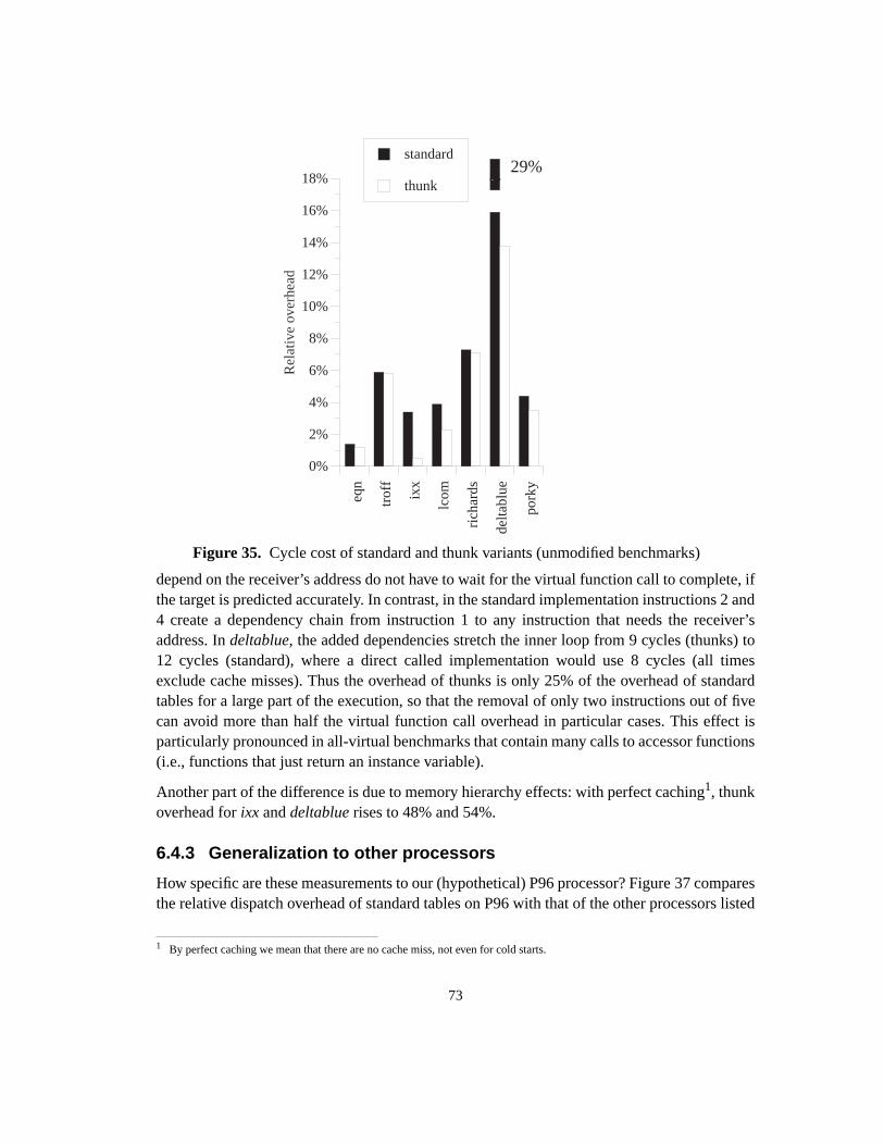
73

depend on the receiver’s address do not have to wait for the virtual function call to complete, ifthe target is predicted accurately. In contrast, in the standard implementation instructions 2 and4 create a dependency chain from instruction 1 to any instruction that needs the receiver’saddress. Indeltablue, the added dependencies stretch the inner loop from 9 cycles (thunks) to12 cycles (standard), where a direct called implementation would use 8 cycles (all timesexclude cache misses). Thus the overhead of thunks is only 25% of the overhead of standardtables for a large part of the execution, so that the removal of only two instructions out of fivecan avoid more than half the virtual function call overhead in particular cases. This effect isparticularly pronounced in all-virtual benchmarks that contain many calls to accessor functions(i.e., functions that just return an instance variable).

Another part of the difference is due to memory hierarchy effects: with perfect caching1, thunkoverhead forixx anddeltablue rises to 48% and 54%.

6.4.3 Generalization to other processors

How specific are these measurements to our (hypothetical) P96 processor? Figure 37 comparesthe relative dispatch overhead of standard tables on P96 with that of the other processors listed

1 By perfect caching we mean that there are no cache miss, not even for cold starts.

Figure 35. Cycle cost of standard and thunk variants (unmodified benchmarks)

eqn

trof

f

ixx

lcom

rich

ards

delta

blue

pork

y

0%

2%

4%

6%

8%

10%

12%

14%

16%

18%

Rel

ativ

e ov

erhe

ad

standard

thunk29%

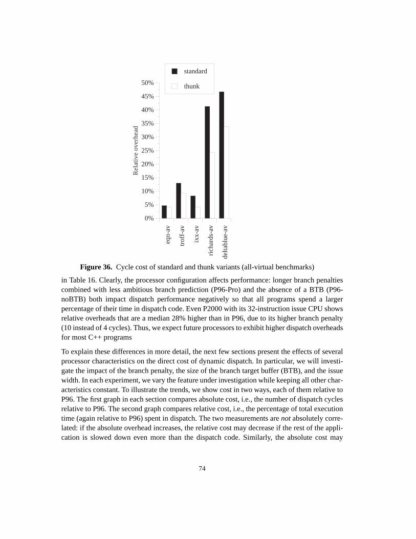
74

in Table 16. Clearly, the processor configuration affects performance: longer branch penaltiescombined with less ambitious branch prediction (P96-Pro) and the absence of a BTB (P96-noBTB) both impact dispatch performance negatively so that all programs spend a largerpercentage of their time in dispatch code. Even P2000 with its 32-instruction issue CPU showsrelative overheads that are a median 28% higher than in P96, due to its higher branch penalty(10 instead of 4 cycles). Thus, we expect future processors to exhibit higher dispatch overheadsfor most C++ programs

To explain these differences in more detail, the next few sections present the effects of severalprocessor characteristics on the direct cost of dynamic dispatch. In particular, we will investi-gate the impact of the branch penalty, the size of the branch target buffer (BTB), and the issuewidth. In each experiment, we vary the feature under investigation while keeping all other char-acteristics constant. To illustrate the trends, we show cost in two ways, each of them relative toP96. The first graph in each section compares absolute cost, i.e., the number of dispatch cyclesrelative to P96. The second graph compares relative cost, i.e., the percentage of total executiontime (again relative to P96) spent in dispatch. The two measurements arenot absolutely corre-lated: if the absolute overhead increases, the relative cost may decrease if the rest of the appli-cation is slowed down even more than the dispatch code. Similarly, the absolute cost may

Figure 36. Cycle cost of standard and thunk variants (all-virtual benchmarks)

eqn-

av

trof

f-av

ixx-

av

rich

ards

-av

delta

blue

-av

0%

5%

10%

15%

20%

25%

30%

35%

40%

45%

50%

Rel

ativ

e ov

erhe

ad

standard

thunk

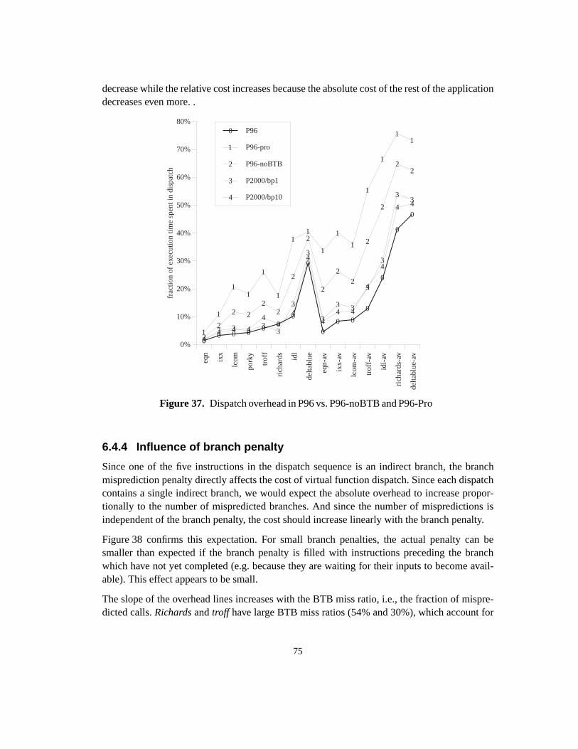
75

decrease while the relative cost increases because the absolute cost of the rest of the applicationdecreases even more. .

6.4.4 Influence of branch penalty

Since one of the five instructions in the dispatch sequence is an indirect branch, the branchmisprediction penalty directly affects the cost of virtual function dispatch. Since each dispatchcontains a single indirect branch, we would expect the absolute overhead to increase propor-tionally to the number of mispredicted branches. And since the number of mispredictions isindependent of the branch penalty, the cost should increase linearly with the branch penalty.

Figure 38 confirms this expectation. For small branch penalties, the actual penalty can besmaller than expected if the branch penalty is filled with instructions preceding the branchwhich have not yet completed (e.g. because they are waiting for their inputs to become avail-able). This effect appears to be small.

The slope of the overhead lines increases with the BTB miss ratio, i.e., the fraction of mispre-dicted calls.Richardsandtroff have large BTB miss ratios (54% and 30%), which account for

Figure 37. Dispatch overhead in P96 vs. P96-noBTB and P96-Pro

00 0 0

0 00

0

00 0

0

0

0

0

1

1

11

1

1

11

1

1

1

1

1

11

2

2

2 2

22

2

2

2

22

2

2

22

33 3 3

33

3

3

3

3 3

3

3

33

44 4 4

44

4

4

44 4

4

4

4 4eq

n

ixx

lcom

pork

y

trof

f

rich

ards id

l

delta

blue

eqn-

av

ixx-

av

lcom

-av

trof

f-av

idl-

av

rich

ards

-av

delta

blue

-av

0%

10%

20%

30%

40%

50%

60%

70%

80%

frac

tion

of e

xecu

tion

time

spen

t in

disp

atch

0 P96

1 P96-pro

2 P96-noBTB

3 P2000/bp1

4 P2000/bp10

76

their steep cost curves. Most of the other benchmarks have a misprediction rate of 10% or less,which dampens the effect of branch penalty on cycle cost.

Figure 39 shows that thefraction of execution time spent in dispatch can actually decrease withincreasing branch penalty. For example,ixx has many indirect calls that are not part of virtualfunction calls, and these branches are very unpredictable (with a BTB miss ratio of 86%).Consequently, the relative overhead of virtual calls inixx decreases with larger branch penaltiessince the cost of the rest of the program increases much faster.

However, for most benchmarks the relative overhead differs less than 20% between the extremebranch penalty values (0 and 10), indicating that the VFT branches are about as predictable asthe other branches in the applications. Thus, the relative dispatch costs given earlier inFigure 33 and Figure 34 are quite insensitive to branch penalty variations.

6.4.5 Influence of branch prediction

As discussed in section 6.2.1, branch target buffers (BTBs) predict indirect (or conditional)branches by storing the target address of the branch’s previous execution. How effective is thisbranch prediction? Our baseline processor, P96, has separate prediction mechanisms for condi-

D D D D D D D D D D D D Dd d d d d d d d d d d d d

EE

EE

EE

EE

EE

EE

E

e e e e e e e e e e e e e

X X X X X X X X X X X X X

x x x x x x x x x x x x xL L L L L L L L L L L L L

l l l l l l l l l l l l lI I I I I I I I I I I I Ii i i i i i i i i i i i i

PP

PP

PP

PP

PP

PP

P

R

R

R

R

R

R

R

R

R

R

R

R

R

r r rr

rr

rr

rr

rr

r

TT

TT

TT

TT

TT

TT

T

t t t t t t t t t t t t t

0 1 2 3 4 5 6 7 8 9 10 11 12

0.5

0.7

0.9

1.1

1.3

1.5

1.7

1.9

2.1

over

head

rel

ativ

e to

P96

branch penalty

D deltablue

d deltablue-av

E eqn

e eqn-av

X ixx

x ixx-av

L lcom

l lcom-av

I idl

i idl-av

P porky

R richards

r richards-av

T troff

t troff-av

Figure 38. Overhead in cycles (relative to P96) for varying branch penalties

77

tional and indirect branches since the former can better be predicted with local history-basedtwo-level predictors [135]. The BTB is used exclusively to predict indirect branches. Thus,

D D D D D D D D D D D D D

d d d d d d d d d d d d d

EE

EE

EE

EE

EE

E

EE

ee e e e e e e e e e e e

XX

XX X

XX X X X

X X X

xx

xx

xx

xx

xx

xx x

L L L L L L L L L L L L L

l l l l l l l l l l l l l

II

II

II

II

II

II

I

i i i i i i i i i i i i iP

PP

PP

PP

PP

PP

PP

R

R

R

R

R

R

R

R

R

R

RR

R

r r r r r r r r r r r r r

T

T

T

T

T

T

T

T

T

T

T

T

T

tt t

t t t t t t t t t t

0 1 2 3 4 5 6 7 8 9 10 11 12

0.6

0.7

0.8

0.9

1

1.1

1.2

1.3

1.4ov

erhe

ad r

elat

ive

to P

96

branch penalty

D deltablue

d deltablue-av

E eqn

e eqn-av

X ixx

x ixx-av

L lcom

l lcom-av

I idl

i idl-av

P porky

R richards

r richards-av

T troff

t troff-av

Figure 39. Overhead in % of execution time (relative to P96) for varying branch penalties

78

varying the size of the BTB will affect only indirect branches, thus directly illustrating theBTB’s effect on dispatch overhead.

In general, smaller BTBs have lower prediction ratios because they cannot store as many indi-vidual branches. Recall that the processor uses the branch instruction’s address to access theBTB (just like a load instruction uses the data address to access the data cache). If the branchisn’t cached in the BTB, it cannot be predicted. Naturally, the smaller the BTB, the fewerbranches it can hold, and thus the larger the fraction of branches that can’t be predicted becausethey aren’t currently cached in the BTB. Figure 40 confirms this expectation: in general, smallerBTBs increase dispatch overhead. Apparently, a BTB size of 128 entries is large enough toeffectively cache all important branches, as the dispatch overhead does not decrease signifi-cantly beyond that BTB size.

DD

D D D D D D D D D

d d d d

d d d d d d d

EE

E EE

E E E E E E

e

e e e

e e e e e e e

X X XX

X

XX X X X X

x x

xx

x

x

x

x

xx x

L

L

L

L

L L L L L L L

l

ll

l

ll

ll l l l

I I I

I I I I I I I I

i i i ii

i i i i i i

P P

P

PP

P P P P P P

R

R R R R R R R R R R

r r r r r

r

r

rr r r

T

TT T

TT T T T T T

tt t t

tt

t

tt t t

0 1 2 4 8 16 32 64 128

256

512

1024

2048

4096

0

1

2

3

4

5

6

over

head

rel

ativ

e to

P96

Branch Target Buffer size

D deltablue

d deltablue-av

E eqn

e eqn-av

X ixx

x ixx-av

L lcom

l lcom-av

I idl

i idl-av

P porky

R richards

r richards-av

T troff

t troff-av

Figure 40. Overhead in cycles (relative to P96) for varying Branch Target Buffer sizes

79

Figure 41 shows the dispatch overhead as a fraction of execution time. In general, the relativeoverhead varies in tandem with the absolute overhead, i.e., smaller BTBs increase dispatchoverhead. For processors with BTBs with 128 or more entries, P96 should accurately predict theBTB’s impact on dispatch performance.

DD

D D D D D D D D D

d d d d

d d d d d d d

EE

E EE

E E E E E E

e

e e e

e e e e e e e

X X XX

X

XX

X X X X

x xx

xx

x

x

x

xx x

L

L

L

L

L L L L L L L

l

ll l

ll

ll l l l

I I I

I I I I I I I I

i i i ii

i i i i i i

P P

P

PP

PP P P P P

R

R R R R R R R R R R

r r r r r rr

r r r r

T

TT T

TT T T T T T

t t t tt

t

t

tt t t

0 1 2 4 8 16 32 64 128

256

512

1024

2048

4096

0

0.5

1

1.5

2

2.5

3

3.5

4

4.5

over

head

rel

ativ

e to

P96

Branch Target Buffer size

D deltablue

d deltablue-av

E eqn

e eqn-av

X ixx

x ixx-av

L lcom

l lcom-av

I idl

i idl-av

P porky

R richards

r richards-av

T troff

t troff-av

Figure 41. Overhead in% of execution time (relative to P96) for varying BTB sizes

80

Finally, Figure 42 shows the prediction ratio as a function of the BTB size. The ratio starts atzero (without a BTB, indirect branches cannot be predicted) and asymptotically reaches a finalvalue around a BTB size of 128. Generally, smaller benchmarks need fewer BTB entries toreach asymptotic behavior since they have fewer active call sites.

The asymptotic prediction ratio corresponds to the hit ratio of an inline cache1 [35]. For somebenchmarks, prediction works very well, with 90% or more of the calls predicted correctly. Butseveral benchmarks (especiallyrichards, ixx, eqn, andtroff) show much lower prediction ratioseven with very large BTBs because their calls change targets too frequently. For example, thesingle virtual call inrichards frequently switches between four different receiver classes, eachof which redefines the virtual function. No matter how large the BTB, such calls cannot bepredicted well. The median prediction ratio for the standard benchmarks is only 76% vs. 92%

1 Since an inline cache stores a target separately for each call site, its hit rate mirrors that of a branch target buffer of infinite sizewith no history prediction bits.

DD

D D D D D D D D D

d d d d

d dd

d

d d d

E

E

E

EE

E E E E E E

e

ee

e

e e e e e e e

X

X X

X

X

X

XX X X X

x x

x

x

x

x

x

x

xx x

L L L

L

L L L L L L L

l l l

l

ll

l

l l l l

I I I

I I I II I I I

i i i i

i

i i i i i i

P

P

P

P

P

PP P P P P

R

R R R R R R R R R R

r r

r r

r

r

r

r

rr r

T

T

TT

T

T T T T T T

t

t t t

t

t

t

t

tt t

0 1 2 4 8 16 32 64 128

256

512

1024

2048

4096

0

10

20

30

40

50

60

70

80

90

100

Hitr

ate

BTB size

D deltablue

d deltablue-av

E eqn

e eqn-av

X ixx

x ixx-av

L lcom

l lcom-av

I idl

i idl-av

P porky

R richards

r richards-av

T troff

t troff-av

Figure 42. Indirect branch prediction ratio as a function of BTB size

81

for the all-virtual versions; the latter are more predictable because many calls only have a singletarget and thus are predicted 100% correctly after the first call.

Indirect branch prediction substantially reduces the average cost of virtual function calls. Insection 6.4.8 we compare average call cost between different prediction regimes.

6.4.6 Influence of load latency

Load latency influences dispatch cost since the VFT dispatch sequence contains two dependentload instructions. Thus, higher load latencies should lead to higher dispatch overhead. Ourmeasurements confirm this assumption: compared to the baseline load latency of two,increasing the load latency to three increases absolute dispatch cost by a median of 51%; therelative cost increases by 31%. Similarly, with a load latency of one the absolute overheaddecreases by 44% and the relative overhead by 37%. (Processors are unlikely to have load laten-cies larger than three, so we did not simulate these.)

Clearly, load latency affects the efficiency of dispatch code more than that of “normal” codesequences. Furthermore, it appears that there are not enough surrounding application instruc-tions to effectively hide the latency of the loads in the dispatch sequence, even for small loadlatencies.

6.4.7 Influence of issue width

The final factor, issue width (i.e., the number of instructions that can be issued to the functionalunits in one cycle) can also influence dispatch performance. Figure 43 shows that issue widthhas a strong impact for small values. On a scalar processor (issuing at most one instruction percycle), programs spend a much smaller fraction of their time in dispatch. Of course, absoluteperformance would be worse than on P96 since execution would consume many more cycles(for example,lcom is three times slower on the one-issue processor than on the four-issueprocessor). With larger issue widths the relative overhead increases more slowly, reaching anasymptotic value of 26% (median) more than on P96. Thus, on wider-issue processors, the rela-tive cost of dynamic dispatch will increase slightly because the application code benefits morefrom the additional issue opportunities than the dispatch code1

1 For a few benchmarks (e.g.,richards) the relative overhead decreases with high issue widths. We assume that these benchmarksbenefit from higher issue rates because they allow critical dispatch instructions to start earlier, thus hiding part of their latency.

82

.

6.4.8 Cost per dispatch

In Section 5.2 we predicted the cost of a single VFT dispatch to be 2L + B + 1, i.e., two loaddelays plus a branch penalty; for P96, this adds up to 9 cycles. How accurate is this prediction?Figure 44 shows the cost in cycles per dispatch for all benchmarks under different BTB predic-tion schemes (no prediction, prediction by a 16-entry BTB, by a 128-entry BTB and withperfect prediction1). No prediction of indirect branches, as in the analytical model, gives amedian overhead of 8.6 cycles, very close to the analytical model, which ignored co-schedulingof non-dispatch instructions. This means that less than one cycle is saved by co-scheduling. Inother words, the virtual function call sequence forms a critical path in the code. Indirect branchprediction can side-step this path, allowing instructions from the predicted target subroutine to

1 The perfect prediction cost was not measured, but estimated from the BTB256 miss rate and the overhead in cycles for BTB256and Noprediction., assuming that the reduction in overhead is proportional to the reduction in miss rate.

Figure 43. Overhead in % of execution time (relative to P96) for varying issue widths

D

D

DD D D D

d

d

dd d d d

E

E

E

EE E E

e

e

e

ee e e

X

X

X

XX

X X

x

x

x

x

x

x x

L

L

L

LL

LL

l

l

l

ll

ll

I

I

I

I I I I

i

i

i

i i i i

P

P

P

P P P P

R

R

R

RR R

R

r

r

r

r rr r

T

T

T

TT T T

t

t

t

t

t

tt

1 2 4 6 8 12 16

0

0.2

0.4

0.6

0.8

1

1.2

1.4

1.6

1.8ov

erhe

ad r

elat

ive

to P

96

Instruction Issue Width

D deltablue

d deltablue-av

E eqn

e eqn-av

X ixx

x ixx-av

L lcom

l lcom-av

I idl

i idl-av

P porky

R richards

r richards-av

T troff

t troff-av

83

execute speculatively, in parallel with the call itself. In this section, we studied this effect forBTB prediction.

A BTB reduces the effective branch penalty since the full penalty B is only incurred upon amisprediction. The analytical cost model could be improved by using the effective branchpenalty Beff = B * btb_misprediction_ratio. For the standard benchmarks, with a medianmisprediction ratio of 24%, this model predicts a cost of 6.0 cycles, which still overestimatesthe real cost (median 3.9 cycles). Considering all benchmarks, the median misprediction ratioof 8% results in an estimated cost of 5.3 cycles per dispatch, which overestimates the actualmedian of 2.8 cycles / dispatch by about a factor two.

Figure 44 demonstrates the importance of indirect branch prediction. Even a small BTB with 16entries reduces the median cost of the standard benchmarks from 8.5 to 4.2 cycles, a factor twoimprovement. A BTB of 256 entries reduces this cost slightly to 3.9 cycles. Beyond 256 entries,a BTB no longer improves prediction accuracy. More sophisticated prediction mechanismshave the potential to reduce call cost by another factor two, as shown by the median 1.6 cyclesper call that results from a perfect (i.e. 100% accurate) predictor.

Dispatch cost varies widely over the different benchmark programs: a single dispatch costs 2.1cycles inlcombut 11.4 cycles indeltablue, a difference of a factor of 5.4. This variation illus-trates the combined effects of the factors discussed previously, such as the BTB hit ratio and the

Figure 44. Cycles per dispatch under various BTB prediction regimes

delta

blue

delta

blue

-av

eqn

eqn-

av ixx

ixx-

av

lcom

lcom

-av idl

idl-a

v

pork

y

richa

rds

richa

rds-

av

trof

f

trof

f-av

0

2

4

6

8

10

12

14

16

18

Cyc

le o

verh

ead

per

virt

ual f

unct

ion

call no prediction

btb16 prediction

btb256 prediction

perfect prediction

84

co-scheduling of application code. The dispatch cost of the all-virtual programs varies muchless since the average cost is dominated by very predictable monomorphic calls (i.e., call sitesinvoking the same function every time).

6.5 Discussion

What does this detailed dispatch performance analysis tell us? Will dispatch performanceimprove with future hardware? Should programmers write their applications differently toimprove performance?

First, the median dispatch overheads we observed for P96 (5.2% for the standard benchmarksand 13.7% for the all-virtual versions) can be used as a bound on the dispatch performanceimprovements one can hope to obtain. Thus, no matter how good a dispatch mechanism is, wecannot hope for much more than a performance improvement of around 5-10% for the C++measured here. Java programs, where all member functions are declared virtual, can gainbetween 5% and 50%. Any further improvement must come from other optimizations such ascustomization or inlining [16][70]. Given that better optimizing compilers are possible [6], ithardly seems appropriate for programmers to compromise the structure of their programs toavoid dispatch.

Many object-oriented systems use or could use VFT-like dispatch mechanisms (e.g., implemen-tations of Java, Modula-3, Oberon-2, and Simula), and thus this study bears some significancefor those languages as well. While the characteristics of typical programs may differ from theC++ programs measured here, the general trends should be similar. Together, the standard andall-virtual programs represent a wide spectrum of program behaviors and call frequencies, andthus we expect many programs written in other languages to fall somewhere within that spec-trum. Furthermore, the dependency structure (and thus performance on superscalar processors)of many other dispatch mechanisms (e.g., selector coloring or row displacement) is similar toVFT, as we have shown in section 5.2. Therefore, the measurements presented here shouldapply to these dispatch mechanisms as well.

Although simulations provide accurate numbers, they are inordinately expensive and compli-cated. As discussed in section 6.4.8, the analytical model for VFT dispatch cost developed insection 5.2 already establishes abound on dispatch cost fairly well using only two parameters.

Finally, will dispatch overhead increase in the future? We believe so. As Figure 43 showed, therelative overhead will increase as processors issue more instructions per cycle. At an issuewidth of 16, the median overhead increases by about 26%. Future processors might also havelonger load latencies, further increasing dispatch cost. General compiler optimizations may alsoinfluence dispatch performance. Much current research focuses on compilation techniques toincrease instruction-level parallelism. If compilers successfully reduce execution time on wide-issue processors, the effective dispatch overhead could further increase for programs withunpredictable VFT calls. The most important aspect of future hardware designs, when it comes

85

to virtual function call cost, is the optimization of indirect branch execution by branch targetprediction. Without target prediction, virtual function calls are twice as expensive, compared toa processor with a sufficiently large BTB. In summary, over the next few years, we expect therelative dispatch cost to rise, though the exact extent is hard to predict.

6.6 Summary

We have analyzed the direct dispatch overhead of the standard virtual function table (VFT)dispatch on a suite of C++ applications with a combination of executable inspection andprocessor simulation. Simulation allows us to precisely define dispatch overhead as the over-head over an ideal dispatch implementation using direct calls only. On average, dispatch over-head is significant: on a processor resembling current superscalar designs, programs spend amedian overhead of 5.2% and a maximum of 29% executing dispatch code. However, many ofthese benchmarks use virtual function calls quite sparingly and thus might underrepresent theactual “average” C++ program. For versions of the programs where every function wasconverted to a virtual function to simulate programming styles that extensively use abstract baseclasses defining virtual functions only (C++’s way of defining interfaces), the median overheadrose to 13.7% and the maximum to 47%. On future processors, this dispatch overhead is likelyto increase moderately.

On average, thunks remove a fourth of the overhead associated with the standard implementa-tion of virtual function calls. For some programs the difference is much higher since thunksremove a data dependency chain that inhibits instruction level parallelism.

To our knowledge, this study is the first one to quantify the direct overhead of dispatch in C++programs, and the first to quantify superscalar effects experimentally. In addition to measuringbottom-line overhead numbers, we have also investigated the influence of specific processorfeatures. Although these features typically influence the absolute dispatch cost considerably(i.e., the number of cycles spent in dispatch code), the relative cost (the percentage of totalexecution time spent in dispatch code) remains fairly constant for most parameters except forextreme values. Thus, the overheads measured here should predict the actual overhead on manycurrent processors reasonably well.

Since many object-oriented languages use virtual function tables for dispatch, and since severalother dispatch techniques have identical execution characteristics on superscalar processors, webelieve that our study applies to these languages as well, especially if their application charac-teristics fall within the range of programs studied here.

Since indirect branch prediction, studied here in the form of a BTB branch target predictor, hassuch a large impact on virtual function call cost (see section 6.4.8), we study indirect branchprediction mechanism in the remainder of this work.

86

87

7 Hardware techniques for efficient polymorphiccalls

“We should give up the attempt to derive resultsand answers with complete certainty”

Michael O.Rabin [115]

In the previous section we established the importance of indirect branch misprediction in thecall cost of virtual functions in C++. Superscalar processors are likely to hide most of the costof table-based polymorphic call resolution by co-scheduling surrounding instructions, but onlywhen the indirect branch is predicted correctly. Since the performance of a branch target buffermaxed out at about 128 entries, more accurate prediction cannot be bought even if a larger tran-sistor budget is available, unless better prediction techniques can be implemented in hardware.Therefore we studied more complex prediction mechanisms in the remainder of this work

7.1 Software vs. hardware prediction

When prediction of indirect branches is unavailable in hardware, software techniques that adaptto observed behavior and predict that it will reoccur can outperform static table-based tech-niques like Virtual Function Table dispatch (VTBL). The latter offer better worst-case perfor-mance but fail to exploit temporal locality at a call site. The simple form of predictionimplemented in an inline cache (jump to the last observed target) is sufficient to achieve betterperformance on average than all forms of dispatch tables on a high-frequency, deeply pipelinedprocessor without indirect branch prediction (Section 5.2).

However, when indirect branch prediction is implemented in a processor’s micro-architecture,table-based techniques become competitive with inline caches. They expose the polymorphismof the call to the hardware prediction architecture in the form of an indirect branch, where theinline cache provides its own prediction in the form of a direct jump. The hardware counterpartof an inline cache is a Branch Target Buffer (BTB). A BTB stores the most recent target addressof a branch.

Inline caching has several advantages over a BTB:

• No cache size limitation: since the predicted target addresses are stored inline, the cachegrows with the program. A BTB is limited in size by the transistor budget allocated tobranch prediction.

• No conflict misses: in an inline cache, every polymorphic call site has its own predictedtarget. A BTB has limited associativity, and will therefore suffer from interference on thebranch address.

• Ease of implementation: an inline cache can easily be combined with other dispatchtechniques. Especially in dynamically typed languages, a slow call resolution technique can

88

be optimized dramatically by placing it as backup technique to an inline cache, with arelatively small programming effort. A BTB requires a static, table-based dispatchtechnique in order to work. In dynamically typed languages, such techniques requiresubstantial implementation effort. They also incur a compile time cost in the form of a tablecompression algorithm (see Section 4).

A BTB, on the other hand, has the following advantages over an inline cache:

• A potentially higher hitrate: if the class of the receiver object of a polymorphic call is notidentical to the last observed class, an inline cache will treat this as a misprediction,even ifthe actual target method is the same (for instance, when the class is a subclass of the lastobserved class and does not override the message definition). A BTB will treat this as a hit(in the absence of conflict and capacity misses).

• A faster miss case: if the inline cache misses, a backup call resolution technique finds thecorrect target and replaces the inlined direct jump target. The instructions that accomplishthis execute in competition with regular code, where hardware-based prediction will updatea call target in parallel, without interfering with regular program execution. A misstherefore incurs a cost bound only by the branch misprediction penalty.

• Greater potential for hit rate improvement: hardware-based prediction can use history-based information, such as the trace of recently executed calls, without slowing downregular execution. As shown in Sections 8 and 9, this information can reduce themisprediction rate by a large factor. Though an inline cache can also use history informationto obtain more accurate prediction, the instructions that maintain this information run incompetition with regular code, implying an extra overhead for every polymorphic call (notjust the miss cases). This does not seem cost-effective.

• Wider applicability: hardware-based indirect branch prediction also speeds up polymorphiccalls in non-object oriented languages (for instance, large switch statements or callsthrough a function pointer table). Even object-oriented programs often execute indirectbranches that are not generated by message dispatch instructions. For example, 52% and66% of the indirect branches inixx and eqn are generated by switch statements (seeTable 17).

In summary, if hardware-based prediction is unavailable or inadequate because of largeprogram working sets, software-based prediction is a good, easy to implement alternative. Withadequate hardware-based prediction, software-based prediction is to be avoided, since it deniesthe hardware the opportunity to do a more accurate prediction with a faster miss case.

89

7.2 Hardware indirect branch prediction

Prediction has a long history in hardware. Caches, filebuffers, RAM disks, virtual memorysystems, disk drivers, all use the principle: what has occurred in the past is likely to occur again,usually pretty soon.

Indirect branch prediction is nothing more than target address caching and prefetching. It isonly a little more specialized than an instruction cache, which, in current practice, alreadyincorporates conditional branch prediction. For example, the UltraSparc I-cache associates a 2-bit counter and a “next” field with every 4 instructions [124]. This field points to the next I-cache line to be fetched if a conditional branch is predicted as taken. The UltraSparc thereforemerges functionality of a BTB with the I-cache. Many of problems we encountered in thecourse of this work resemble problems encountered in cache design. For example, many of thesolutions in Section 8 come straight out of cache design literature [65]. Others are inspired bygood conditional branch designs, for example the GSHARE predictor [98].

To see which of these solutions carry over to indirect branch predictors, we have to measuretheir predictor performance on real programs. We use misprediction rate, defined as branchmisprediction/frequency, as the metric to evaluate designs. Minimization of misprediction rateensures that often executed branches carry more weight.

7.3 Indirect branch frequency

How important are indirect branches? We answered this question partly in the previous section,since every virtual function call in C++ has an indirect branch as its core instruction. The over-head of 5% and 14%, was mostly due to mispredicted indirect branches, since the other instruc-tions have no large impact on performance. However, not all indirect branches correspond tovirtual function calls. Of the seven C++ programs in our benchmark suite, discussed in the nextsection, two execute more switch statements than virtual function calls. In non-object orientedlanguages, the only way to have polymorphic calls is to hand-code polymorphic call resolutionprocedures, which use large switch statements or function pointer tables, both of whichgenerate indirect branches.

7.3.1 Benchmark overview

Our main benchmark suite consists of large object-oriented C++ applications ranging from8,000 to over 75,000 non-blank lines of C++ code each (see Table 17), andbeta, a compiler forthe Beta programming language [90], written in Beta. We also measured the SPECint95 bench-mark suite with the exception ofcompress which executes only 590 branches during acomplete run. Together, the benchmarks represent over 500,000 non-comment source lines.

All C and C++ programs exceptself 1 were compiled with GNU gcc 2.7.2 (options -O2 -multrasparc plus static linking) and run under theshade instruction-level simulator [29] to

90

obtain traces of all indirect branches. Procedure returns were excluded because they can bepredicted accurately with a return address stack [82]. All programs were run to completion oruntil six million indirect branches were executed.1 In jhm andself we excluded the initializa-tion phases by skipping the first 5 and 6 million indirect branches, respectively.

For each benchmark, Table 17 lists the number of indirect branches executed, the number ofinstructions executed per indirect branch, the number of conditional branches executed per indi-rect branch, and the percentage of indirect branch executions that correspond to the branchclasses used in Section 9.2.1 and Section 9.2.2, as well as the number of branch sites respon-sible for 99%, and 100% of the branch executions. For example, only 5 different branch sites areresponsible for 99% of the dynamic indirect branches ingo. The SPECint95 programs aredominated by very few indirect branches, with less than ten interesting branches for allprograms exceptgcc . Four of the SPEC benchmarks execute more than 1,000 instructions perindirect branch. Since the impact of branch prediction will be very low for the latter four bench-marks, we exclude them when optimizing predictor performance (by minimizing the AVGmisprediction rate).

1 self does not execute correctly when compiled with -O2 and was thus compiled with “-O” optimization. Also,self was notfully statically linked; our experiments exclude instructions executed in dynamically-linked libraries.1 We reduced the traces of three of the SPEC benchmarks in order to reduce simulation time. In all of these cases, the BTBmisprediction rate differs by less than 1% (relative) between the full and truncated traces, and thus we believe that the resultsobtained with the truncated traces are accurate.

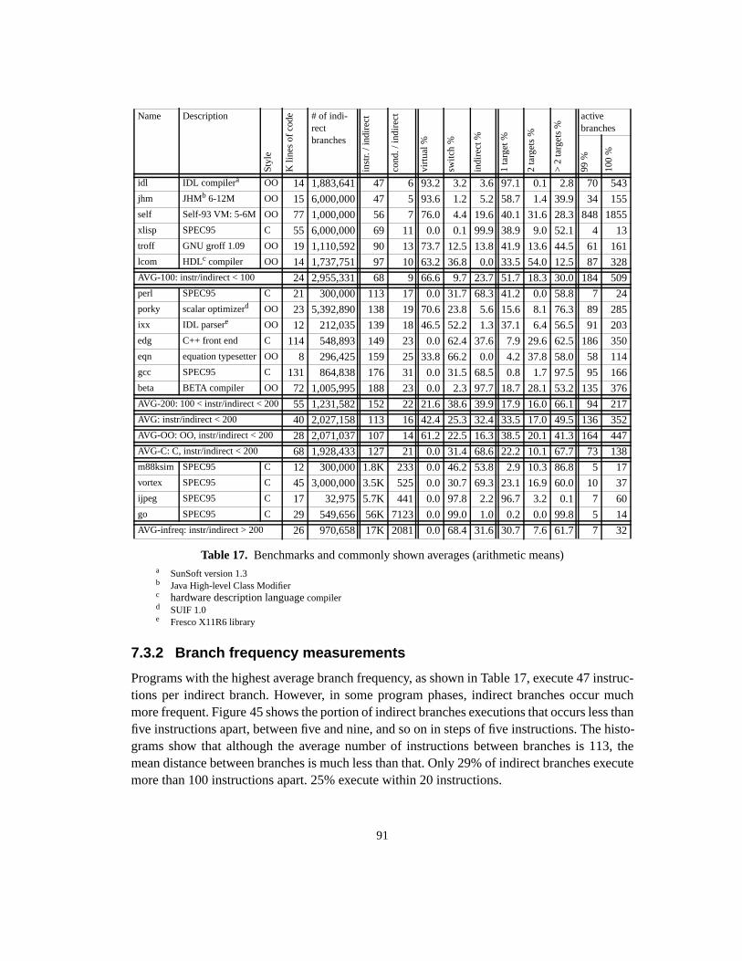
91

7.3.2 Branch frequency measurements

Programs with the highest average branch frequency, as shown in Table 17, execute 47 instruc-tions per indirect branch. However, in some program phases, indirect branches occur muchmore frequent. Figure 45 shows the portion of indirect branches executions that occurs less thanfive instructions apart, between five and nine, and so on in steps of five instructions. The histo-grams show that although the average number of instructions between branches is 113, themean distance between branches is much less than that. Only 29% of indirect branches executemore than 100 instructions apart. 25% execute within 20 instructions.

a SunSoft version 1.3b Java High-level Class Modifierc hardware description language compilerd SUIF 1.0e Fresco X11R6 library

Name Description

Sty

le

K li

nes

of c

ode # of indi-

rectbranches

inst

r. / i

ndire

ct

cond

. / in

dire

ct

virt

ual %

switc

h %

indi

rect

%

1 ta

rget

%

2 ta

rget

s %

> 2

targ

ets

% activebranches

99 %

100

%

idl IDL compilera OO 14 1,883,641 47 6 93.2 3.2 3.6 97.1 0.1 2.8 70 543jhm JHMb 6-12M OO 15 6,000,000 47 5 93.6 1.2 5.2 58.7 1.4 39.9 34 155self Self-93 VM: 5-6M OO 77 1,000,000 56 7 76.0 4.4 19.6 40.1 31.6 28.3 848 1855xlisp SPEC95 C 55 6,000,000 69 11 0.0 0.1 99.9 38.9 9.0 52.1 4 13troff GNU groff 1.09 OO 19 1,110,592 90 13 73.7 12.5 13.8 41.9 13.6 44.5 61 161lcom HDLc compiler OO 14 1,737,751 97 10 63.2 36.8 0.0 33.5 54.0 12.5 87 328AVG-100: instr/indirect < 100 24 2,955,331 68 9 66.6 9.7 23.7 51.7 18.3 30.0 184 509perl SPEC95 C 21 300,000 113 17 0.0 31.7 68.3 41.2 0.0 58.8 7 24porky scalar optimizerd OO 23 5,392,890 138 19 70.6 23.8 5.6 15.6 8.1 76.3 89 285ixx IDL parsere OO 12 212,035 139 18 46.5 52.2 1.3 37.1 6.4 56.5 91 203edg C++ front end C 114 548,893 149 23 0.0 62.4 37.6 7.9 29.6 62.5 186 350eqn equation typesetter OO 8 296,425 159 25 33.8 66.2 0.0 4.2 37.8 58.0 58 114gcc SPEC95 C 131 864,838 176 31 0.0 31.5 68.5 0.8 1.7 97.5 95 166beta BETA compiler OO 72 1,005,995 188 23 0.0 2.3 97.7 18.7 28.1 53.2 135 376AVG-200: 100 < instr/indirect < 200 55 1,231,582 152 22 21.6 38.6 39.9 17.9 16.0 66.1 94 217AVG: instr/indirect < 200 40 2,027,158 113 16 42.4 25.3 32.4 33.5 17.0 49.5 136 352AVG-OO: OO, instr/indirect < 200 28 2,071,037 107 14 61.2 22.5 16.3 38.5 20.1 41.3 164 447AVG-C: C, instr/indirect < 200 68 1,928,433 127 21 0.0 31.4 68.6 22.2 10.1 67.7 73 138m88ksim SPEC95 C 12 300,000 1.8K 233 0.0 46.2 53.8 2.9 10.3 86.8 5 17vortex SPEC95 C 45 3,000,000 3.5K 525 0.0 30.7 69.3 23.1 16.9 60.0 10 37ijpeg SPEC95 C 17 32,975 5.7K 441 0.0 97.8 2.2 96.7 3.2 0.1 7 60go SPEC95 C 29 549,656 56K 7123 0.0 99.0 1.0 0.2 0.0 99.8 5 14AVG-infreq: instr/indirect > 200 26 970,658 17K 2081 0.0 68.4 31.6 30.7 7.6 61.7 7 32

Table 17. Benchmarks and commonly shown averages (arithmetic means)

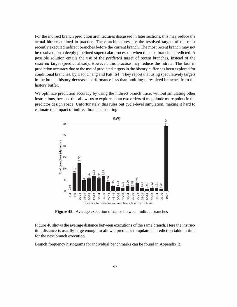
92

For the indirect branch prediction architectures discussed in later sections, this may reduce theactual hitrate attained in practice. These architectures use the resolved targets of the mostrecently executed indirect branches before the current branch. The most recent branch may notbe resolved, on a deeply pipelined superscalar processor, when the next branch is predicted. Apossible solution entails the use of thepredicted target of recent branches, instead of theresolved target (predict ahead). However, this practise may reduce the hitrate. The loss inprediction accuracy due to the use of predicted targets in the history buffer has been explored forconditional branches, by Hao, Chang and Patt [64]. They report that using speculatively targetsin the branch history decreases performance less than omitting unresolved branches from thehistory buffer.

We optimize prediction accuracy by using the indirect branch trace, without simulating otherinstructions, because this allows us to explore about two orders of magnitude more points in thepredictor design space. Unfortunately, this rules out cycle-level simulation, making it hard toestimate the impact of indirect branch clustering

Figure 46 shows the average distance between executions of the same branch. Here the instruc-tion distance is usually large enough to allow a predictor to update its prediction table in timefor the next branch execution.

Branch frequency histograms for individual benchmarks can be found in Appendix B.

0-4

5-9

10-

14

15-

19

20-

24

25-

29

30-

34

35-

39

40-

44

45-

49

50-

54

55-

59

60-

64

65-

69

70-

74

75-

79

80-

84

85-

89

90-

94

95-

99

100+

0

5

10

15

20

25

30

% o

f bra

nche

s (d

ynam

ic)

Distance to previous indirect branch in instructions

0.01

8.14

12.3

6

4.8 5.47 6.

62

5.54 6.

65

3.86

1.96

1.74

1.25 2.

06

1.87 3.

28

1.28

0.93

1.12

1.21

1.01

28.8

5avg

Figure 45. Average execution distance between indirect branches

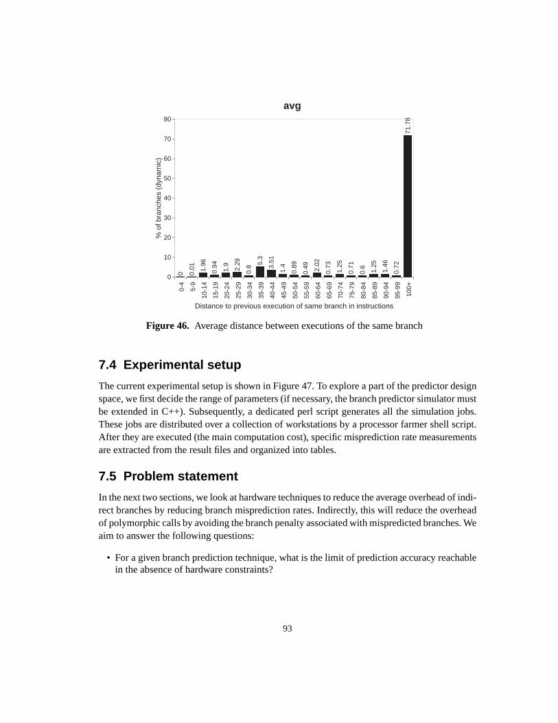
93

7.4 Experimental setup

The current experimental setup is shown in Figure 47. To explore a part of the predictor designspace, we first decide the range of parameters (if necessary, the branch predictor simulator mustbe extended in C++). Subsequently, a dedicated perl script generates all the simulation jobs.These jobs are distributed over a collection of workstations by a processor farmer shell script.After they are executed (the main computation cost), specific misprediction rate measurementsare extracted from the result files and organized into tables.

7.5 Problem statement

In the next two sections, we look at hardware techniques to reduce the average overhead of indi-rect branches by reducing branch misprediction rates. Indirectly, this will reduce the overheadof polymorphic calls by avoiding the branch penalty associated with mispredicted branches. Weaim to answer the following questions:

• For a given branch prediction technique, what is the limit of prediction accuracy reachablein the absence of hardware constraints?

0-4

5-9

10-

14

15-

19

20-

24

25-

29

30-

34

35-

39

40-

44

45-

49

50-

54

55-

59

60-

64

65-

69

70-

74

75-

79

80-

84

85-

89

90-

94

95-

99

100+

0

10

20

30

40

50

60

70

80

% o

f bra

nche

s (d

ynam

ic)

Distance to previous execution of same branch in instructions

0 0.01 1.

96

0.94 1.9

2.29

0.8 5.

3

3.51

1.4

0.89

0.49 2.02

0.73

1.25

0.71

0.6

1.25

1.46

0.72

71.7

8

avg

Figure 46. Average distance between executions of the same branch

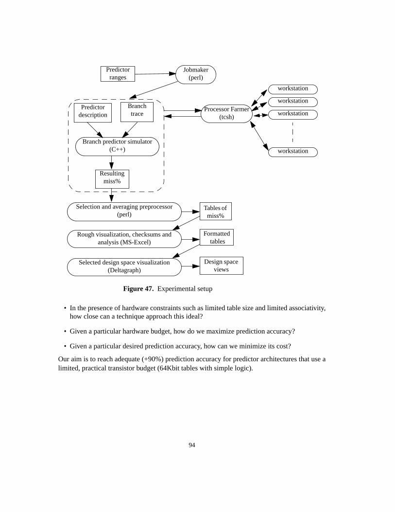
94

• In the presence of hardware constraints such as limited table size and limited associativity,how close can a technique approach this ideal?

• Given a particular hardware budget, how do we maximize prediction accuracy?

• Given a particular desired prediction accuracy, how can we minimize its cost?

Our aim is to reach adequate (+90%) prediction accuracy for predictor architectures that use alimited, practical transistor budget (64Kbit tables with simple logic).

Predictordescription

Branchtrace

Branch predictor simulator(C++)

Resultingmiss%

Jobmaker(perl)

Predictorranges

Processor Farmer(tcsh)

Selection and averaging preprocessor(perl)

Tables ofmiss%

Rough visualization, checksums andanalysis (MS-Excel)

Formatted tables

Selected design space visualization(Deltagraph)

Design spaceviews

Figure 47. Experimental setup

workstation

workstation

workstation

workstation

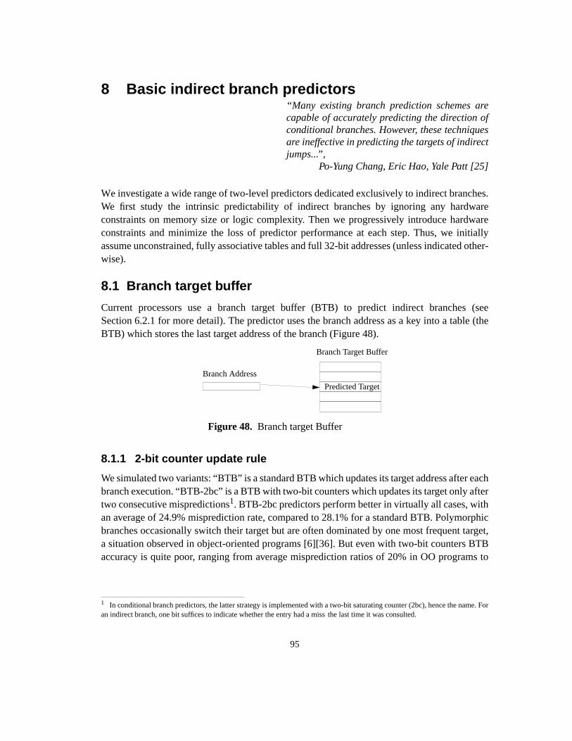
95

8 Basic indirect branch predictors“Many existing branch prediction schemes arecapable of accurately predicting the direction ofconditional branches. However, these techniquesare ineffective in predicting the targets of indirectjumps...”,

Po-Yung Chang, Eric Hao, Yale Patt [25]

We investigate a wide range of two-level predictors dedicated exclusively to indirect branches.We first study the intrinsic predictability of indirect branches by ignoring any hardwareconstraints on memory size or logic complexity. Then we progressively introduce hardwareconstraints and minimize the loss of predictor performance at each step. Thus, we initiallyassume unconstrained, fully associative tables and full 32-bit addresses (unless indicated other-wise).

8.1 Branch target buffer

Current processors use a branch target buffer (BTB) to predict indirect branches (seeSection 6.2.1 for more detail). The predictor uses the branch address as a key into a table (theBTB) which stores the last target address of the branch (Figure 48).

8.1.1 2-bit counter update rule

We simulated two variants: “BTB” is a standard BTB which updates its target address after eachbranch execution. “BTB-2bc” is a BTB with two-bit counters which updates its target only aftertwo consecutive mispredictions1. BTB-2bc predictors perform better in virtually all cases, withan average of 24.9% misprediction rate, compared to 28.1% for a standard BTB. Polymorphicbranches occasionally switch their target but are often dominated by one most frequent target,a situation observed in object-oriented programs [6][36]. But even with two-bit counters BTBaccuracy is quite poor, ranging from average misprediction ratios of 20% in OO programs to

1 In conditional branch predictors, the latter strategy is implemented with a two-bit saturating counter (2bc), hence the name. Foran indirect branch, one bit suffices to indicate whether the entry had a miss the last time it was consulted.

Figure 48. Branch target Buffer

Branch Target Buffer

Branch Address

Predicted Target

96

37% for C programs. Infrequent indirect branches (AVG-200) are less predictable, with amisprediction average of 38% vs. 10% for the programs in AVG-100.

8.2 Two-level predictor

Two-level predictors improve prediction accuracy by keeping information from previousbranch executions in a history buffer. Combined with the branch address, this history pattern isused as a key into the History Table which contains the predicted target addresses. As in BTBs,the entries can be updated on every miss or after two consecutive misses (2-bit counters). Wetested every predictor in this section with both variants, and always saw a slight improvementwith 2-bit counters. I.e., ignoring a stand-alone miss when updating seems to be a good strategyin general. Thus, we will only show 2-bit counter results in the rest of the paper.

Figure 49. Indirect branch misprediction rates for an unconstrained BTB

idl

jhm

self

troff

lcom

pork

y

ixx

eqn

beta

AV

G-O

O

xlis

p

perl

edg

gcc

AV

G-C

AV

G-1

00

AV

G-2

00

AV

G

m88ks

im

vort

ex

ijpeg

go

AV

G-infr

eq

0%

10%

20%

30%

40%

50%

60%

70%

80%

90%

100%M

ispre

dic

tion r

ate

BTB

BTB-2bc

History Pattern (p targets)

History Table

Figure 50. Two-level branch prediction

Branch AddressKey Predicted Target

97

For conditional branches, a branch history of lengthp consists of the taken/not-taken bits of thep most recently executed branches [135]. In contrast, most indirect branches are unconditional,and thus keeping a history of taken/not-taken bits would be ineffective. Instead, the history mustconsist of previous target addresses or bits thereof. Such a path-based history could also be usedto predict conditional branches, but since taken/not-taken bits succinctly summarize the targetaddresses of a conditional branch, conditional branch predictors usually do not employ targetaddress histories (but see [105]).

8.2.1 First level: history pattern

Branch predictors can use one or more history buffers. Aglobal history uses a single historybuffer (correlation branch prediction), and all branches are predicted using the outcomes of thep most recently executed branches. In contrast, aper-address history keeps a separate historyfor each branch, so that branches do not influence each other’s prediction. Finally,per-sethistory prediction forms a compromise by using a separate history for each set of branches,where a set may be determined by the branch opcode, a compiler-assigned branch class, or aparticular address range (see Yeh and Patt’s comprehensive study [135]).

To investigate the impact of global vs. local histories, we simulated per-set histories where a setcontains all branches in a memory region of size 2s bytes, i.e., all branches with the same valuesin bitss..31 fall into the same set (Figure 51). With this parametrization, a global history corre-

sponds tos=31, and per-branch histories correspond tos=2. Using the results of the exhaustive

History Patterns

Figure 51. History pattern sharing

Branch Address

Key (concatenate)

s

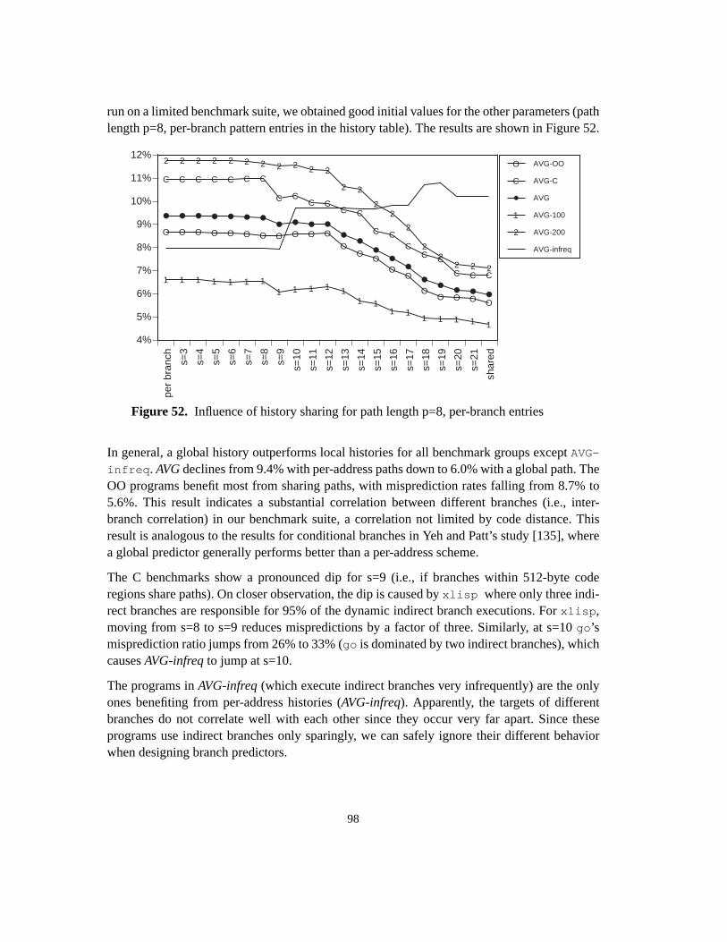
98

run on a limited benchmark suite, we obtained good initial values for the other parameters (pathlength p=8, per-branch pattern entries in the history table). The results are shown in Figure 52.

In general, a global history outperforms local histories for all benchmark groups exceptAVG-

infreq . AVG declines from 9.4% with per-address paths down to 6.0% with a global path. TheOO programs benefit most from sharing paths, with misprediction rates falling from 8.7% to5.6%. This result indicates a substantial correlation between different branches (i.e., inter-branch correlation) in our benchmark suite, a correlation not limited by code distance. Thisresult is analogous to the results for conditional branches in Yeh and Patt’s study [135], wherea global predictor generally performs better than a per-address scheme.

The C benchmarks show a pronounced dip for s=9 (i.e., if branches within 512-byte coderegions share paths). On closer observation, the dip is caused byxlisp where only three indi-rect branches are responsible for 95% of the dynamic indirect branch executions. Forxlisp ,moving from s=8 to s=9 reduces mispredictions by a factor of three. Similarly, at s=10go ’smisprediction ratio jumps from 26% to 33% (go is dominated by two indirect branches), whichcausesAVG-infreq to jump at s=10.

The programs inAVG-infreq (which execute indirect branches very infrequently) are the onlyones benefiting from per-address histories (AVG-infreq). Apparently, the targets of differentbranches do not correlate well with each other since they occur very far apart. Since theseprograms use indirect branches only sparingly, we can safely ignore their different behaviorwhen designing branch predictors.

Figure 52. Influence of history sharing for path length p=8, per-branch entries

O O O O O O O O O O O

OO

OO

O

OO O O O

C C C C C C C

C CC C

C C

C CC

C C

C C C1 1 1 1 1 1 11 1 1 1 1

1 11 1

1 1 1 1 1

2 2 2 2 2 2 2 2 2 2 2

2 2

22

2

22

2 2 2

per

bran

ch s=3

s=4

s=5

s=6

s=7

s=8

s=9

s=10

s=11

s=12

s=13

s=14

s=15

s=16

s=17

s=18

s=19

s=20

s=21

shar

ed

4%

5%

6%

7%

8%

9%

10%

11%

12%O AVG-OO

C AVG-C

AVG

1 AVG-100

2 AVG-200

AVG-infreq

99

8.2.2 Second level: history table sharing

A two-level predictor uses the history pattern to index into a history table that stores predictedtargets. Again, we have a choice of per-branch, per-set, or global prediction. We simulated per-set tables that grouped all branches with identical address bitsh..31 into the same set (seeFigure 53). Thus,h=2 implies per-branch history tables (each branch has its own history table)

andh=31 implies a single shared history table (i.e., all branches with the same history share thesame prediction). Figure 54 shows that the branch address matters: The misprediction average

for all benchmarks increases from 6.0% for per-address history tables to 9.6% for a globallyshared history table, the rate of the OO programs increases from 5.6% to 8.6%, and that of theC benchmarks rises from 6.8% to 11.8%. (Again,xlisp changes dramatically ath=9, causing asharp increase for some averages.) Therefore, we will only consider per-address tables (h=2) insubsequent experiments.

Global History Pattern

Figure 53. History Table sharing

Branch Address

h

Key (concatenate)

Figure 54. Influence of history table sharing for path length 8 with a global history pattern.

O O O O O O O O O O O O O O O OO O O O O

C C C C C C C

C C C C C C C C C C C C C C

1 1 1 1 1 1 1

1 1 1 1 1 1 1 1 11 1 1 1 1

2 2 2 2 2 2 2 2 2 2 2 2 2 22 2

2 2 2 2 2

per

bran

ch

h=3

h=4

h=5

h=6

h=7

h=8

h=9

h=10

h=11

h=12

h=13

h=14

h=15

h=16

h=17

h=18

h=19

h=20

h=21

shar

ed

4%

6%

8%

10%

12%

14%

16%

18%O AVG-OO

C AVG-C

AVG

1 AVG-100

2 AVG-200

AVG-infreq

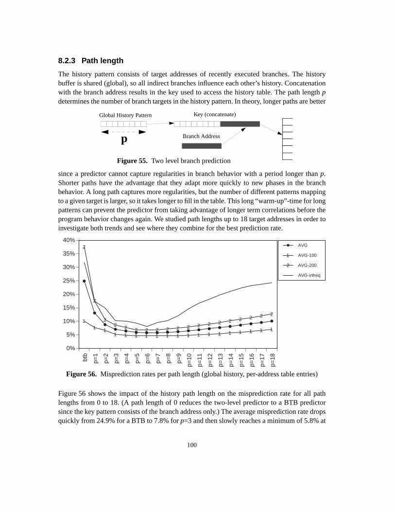
100

8.2.3 Path length

The history pattern consists of target addresses of recently executed branches. The historybuffer is shared (global), so all indirect branches influence each other’s history. Concatenationwith the branch address results in the key used to access the history table. The path lengthpdetermines the number of branch targets in the history pattern. In theory, longer paths are better

since a predictor cannot capture regularities in branch behavior with a period longer thanp.Shorter paths have the advantage that they adapt more quickly to new phases in the branchbehavior. A long path captures more regularities, but the number of different patterns mappingto a given target is larger, so it takes longer to fill in the table. This long “warm-up”-time for longpatterns can prevent the predictor from taking advantage of longer term correlations before theprogram behavior changes again. We studied path lengths up to 18 target addresses in order toinvestigate both trends and see where they combine for the best prediction rate.

Figure 56 shows the impact of the history path length on the misprediction rate for all pathlengths from 0 to 18. (A path length of 0 reduces the two-level predictor to a BTB predictorsince the key pattern consists of the branch address only.) The average misprediction rate dropsquickly from 24.9% for a BTB to 7.8% forp=3 and then slowly reaches a minimum of 5.8% at

Figure 55. Two level branch prediction

Branch Address

Key (concatenate)Global History Pattern

p

Figure 56. Misprediction rates per path length (global history, per-address table entries)

11 1

1 1 1 1 1 1 1 1 1 1 1 1 1 1 1 1

2

2

22 2 2 2 2 2 2 2 2 2 2 2 2 2 2 2

btb

p=1

p=2

p=3

p=4

p=5

p=6

p=7

p=8

p=9

p=10

p=11

p=12

p=13

p=14

p=15

p=16

p=17

p=18

0%

5%

10%

15%

20%

25%

30%

35%

40%AVG

1 AVG-100

2 AVG-200

AVG-infreq

101

path length 6. Then the misprediction rate starts to rise again and keeps rising for larger pathlengths up to the limit of our testing range atp=18. All benchmark suites follow this pattern,although programs with infrequent branches show uniformly higher misprediction rates.

This result indicates that most regularities in the indirect branch traces have a relatively shortperiod. In other words, a predictable indirect branch execution is usually correlated with theexecution of less than three branches before it. Increasing the path length captures some longerterm correlations, but at path length six cold-start misses begin to negate the advantage of alonger history. At this point, adding an extra branch target to the path may still allow longer-term correlations to be exploited, but on the other hand it will take the branch predictor longerto learn a full new pattern association for every branch that changes its behavior due to a phasetransition in the program. A hybrid branch predictor combining both short and long pathcomponents should be able to adapt quickly to phase changes while still exploiting longer-termcorrelations; we experiment with such hybrid predictors in Section 9.

8.3 History buffers

8.3.1 Trace information

We explored a few other choices for the history pattern elements. In the first variant we usedboth branch address and target, and in the second we included targets of conditional branchesin the history. Both resulted in inferior prediction accuracy1 for any pattern lengthp (see [46]).

8.3.2 History pattern compression

The global history pattern is a very long bit pattern. For p=8, it consists of 8 * 32 = 256 bits, andconcatenation with the branch address results in a total of 288 bits. The information content ofthis bit pattern is quite low: the number of different patterns that occur during program execu-tion is much smaller than 2288. Since a tag in an associative table includes most of the pattern,long patterns inflate the size of the predictor table. We need to compress the pattern for eachpath length into a short bit pattern, ideally without compromising prediction accuracy. As a firststep towards smaller history patterns, we will only consider path lengths up to sizep=12, sincelonger path lengths result in higher misprediction rates (as seen in Figure 56)

8.3.2.1 Target pattern projection

A straightforward approach for history pattern compression is to select a limited number of bitsfrom each target and concatenate these partial addresses into the history pattern. We explored a

1 This result is often misunderstood. It does not say that conditional branches are irrelevant to indirect branch prediction. It saysthat, given a the choice of tracing the last n indirect branches or the last n conditional branches, the indirect branches predict thenext indirect branch better. For some individual branches this may be wrong (as suggested by Kalamatianos and Kaeli [81], whodynamically choose a pure indirect or a mixed conditional/indirect trace for each branch), but over the whole benchmark suite, thistrend holds.

102

number of choices by using a range [a..A] of the address bits. We varieda from 2 to 10, andAfrom a to a+(b-1), whereb is the largest number of bits that still allows the history pattern to fitwithin a total of 24 bits (i.e.b * p <= 24). Starting with bita=2 worked best on average, and thuswe will not show data for other values of a.

Figure 57 shows the misprediction ratios resulting from the selection of bits [2..2+(b-1)], for bvalues of 1,2,3,4 and 8, as well as the misprediction rate for full-precision addresses. The curvefor b=8 almost completely overlaps with the full-address curve, indicating that 8 bits are enougheven for short path lengths. For decreasing address precision, shorter path lengths suffer most.For example, for path length p=10, 2 bits achieve a misprediction rate of 6.77% vs. 6.53% forfull addresses, while for path length p=3, the miss ratio decreases from 10.6% (2 bits) to 7.1%(full addresses). A total bit length of 24 bits suffices for the history pattern to approach the full-address performance for all path lengths. Thus, in the rest of the paper we always choose thelargest numberb of bits from each address that keepsb * p <= 24. For example, for path length2 we choose 12 bits for each history entry, and for path length 6 we choose 4.

We also tried two other schemes for target address compression:

• Fold the new target address into the desired number ofb bits by dividing it into chunks ofb bits and xor-ing them all together.

• Shift the history patternb bits to the left and xor with the complete new target address.

Figure 57. Limited Precision misprediction rates.

1

1

11

11

1 1 1 1 1 1

2

2

22

22 2 2 2 2 2 2

3

3

33

3 3 3 3

4

4

44

4 4

8

8

8

p=1

p=2

p=3

p=4

p=5

p=6

p=7

p=8

p=9

p=10

p=11

p=12

0%

5%

10%

15%

20%

25%1 1 bit

2 2 bit

3 3 bit

4 4 bit

8 8 bit

full address

AVG for 1, 2, 3, 4, 8 bit and full target addresses.(low order bits starting from bit 2)

103

These variants were intended to use more information of the target address but did not reliablyresult in better prediction rates and were sometimes even worse. Since they require more logicthan the bit selection discussed above, we decided to drop them from further tests1.

8.3.2.2 Address folding

As mentioned in section 8.2.2, omitting the branch address reduces the performance of a two-level predictor (for p=8, the misprediction rate increased from 6.0% to 9.6%). However, concat-enating the branch address with the history pattern results in a key of 24 + 30 = 54 bits. Inanalogy with theGshare predictor used in conditional branch prediction [24], we can reduce thenumber of bits in the key pattern to 30 by xor-ing the branch address with the history pattern.Table 18 shows the misprediction rate averages for both alternatives. Compared to the increase

in misprediction rate due to limited table size and associativity in the next section, the reductionof the key pattern from 54 to 30 bits by xor causes a very small increase in misprediction rate.For example, for path length 8, misprediction rate increases by 0.03%, from 6.16% to 6.19%Since this operation reduces the table space used for tag bits by more than half, we use thisscheme in the remainder of this study.

8.4 History tables

In this section we introduce limited table sizes and limited associativity in order to obtain prac-tical indirect branch predictors.

8.4.1 Capacity misses

Limited tables introduce a new source of branch misses: capacity misses. When the table is toosmall to store the history patterns of all branches in its working set, some patterns will beevicted from the table, resulting in capacity misses.

Longer path lengths generate more patterns for a given set of branches. For example,ixx gener-ates 203 different patterns for path lengthp=0, 402 forp=1, 865 forp=2, 1469 forp=3, and ends

1 Since the difference in prediction accuracy between partial bit-selected addresses and full-precision addresses is already verysmall, there is not much to be gained by sophisticated hashing schemes. We measured a difference of 0.2%, when going from afullprecision path length 6 to a 4-bit path length 6 predictor. One could hope for positive interference, but this is much less likelyto occur in indirect branch prediction than in conditional branch prediction, since the predicted value is a 32bit address, not just abit (which is 50% likely to positively interfere on a miss).

Operation p=0 p=1 p=2 p=3 p=4 p=5 p=6 p=7 p=8 p=9 p=10 p=11 p=12

Xor 24.91 13.58 8.84 7.09 6.49 6.27 6.01 6.18 6.19 7.44 7.34 7.49 7.67

Concat 24.91 13.08 8.78 7.08 6.48 6.22 5.99 6.13 6.16 6.62 6.77 7.02 7.27

difference 0.00 0.50 0.06 0.01 0.01 0.05 0.02 0.05 0.03 0.82 0.57 0.47 0.40

Table 18. Concatenation versus Xor of history pattern with branch address (AVG)

104

up with 9403 patterns forp=12. Though not all patterns are used more than once (some onlyoccur once in the warm-up phase), for longer path lengths capacity misses will occur fairlysoon. A predictor with a longer path length may be more accurate than a predictor of shorterpath length for an unlimited table, but the capacity misses caused by a small table size can affectthe longer path length predictor enough to negate this advantage.

To estimate the effect of capacity misses we simulate fully-associative tables with LRU replace-ment policy. Figure 58 shows the average misprediction rate for various fully-associative tablesfor predictors with path length p=0-4,6,8,10 and 12. The misprediction rate of some pathlengths reaches its minimum in the explored range. For p=0 (BTB), the miss rate decreases withincreasing table size and reaches its minimum at 256 entries. Since there are no capacity missesleft, increasing the table size beyond this point will not lower the miss rate for p=0. Increasingthe path lengths pushes this point out to 1024 entries (p=1), 2048 entries (p=2), and 8192 entries(p=3 and p=4). Longer path lengths never completely recover from capacity misses in theexplored range. A longer path’s ability to detect longer-term regularities can pay off, althoughthe best predictor for each table size is still affected by capacity misses. For instance, p=2 winsat table size 256 with a misprediction rate of 12.5%, 3.6% of which is due to capacity misses.For size 1024, p=3 takes over with a misprediction rate of 8.5%, with 1.4% due to capacitymisses. For a 8192-entry table, p=6 (which achieved the lowest misprediction rate for an unlim-ited table) has a misprediction rate of 6.6%, with 0.6% due to capacity misses.

8.4.2 Conflict misses

In practice, a fully-associative LRU table of sufficient size requires too much logic to imple-ment in hardware, and thus we will explore limited-associative tables in this section.

1 1 1 1 1 1

2

22

2 2 2

3

33

33 3

4

4

44

4 4

6

6

6

6

66

8

8

8

8

8

a

a

a

a

c

c

c

512

1024

2048

4096

8192

Unl

imite

d

5%

6%

7%

8%

9%

10%

11%

12%

13%

14%

15%0 btb

1 p=1

2 p=2

3 p=3

4 p=4

6 p=6

8 p=8

a p=10

c p=12

00

0 0 0 0 0 0 0 0

1

11

1 1 1 1 1 1 1

2

2

2

22 2 2 2 2 2

3

3

3

33 3 3 3 3

4

4

4

4

44 4 4 4

6

6

6

6

66

6 6

8

8

8

88

88

a

a

a

a

aa

a

c

c

c

cc

c

32 64 128

256

512

1024

2048

4096

8192

Unl

imite

d

0%

5%

10%

15%

20%

25%

30%

Figure 58. AVG of limited size fully-associative misprediction ratios

LRU replacement policy(cut-out section enlarged in right graph)

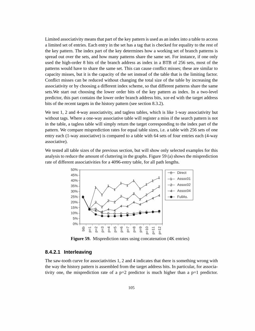
105

Limited associativity means that part of the key pattern is used as an index into a table to accessa limited set of entries. Each entry in the set has a tag that is checked for equality to the rest ofthe key pattern. The index part of the key determines how a working set of branch patterns isspread out over the sets, and how many patterns share the same set. For instance, if one onlyused the high-order 8 bits of the branch address as index in a BTB of 256 sets, most of thepatterns would have to share the same set. This can cause conflict misses; these are similar tocapacity misses, but it is the capacity of the set instead of the table that is the limiting factor.Conflict misses can be reduced without changing the total size of the table by increasing theassociativity or by choosing a different index scheme, so that different patterns share the samesets.We start out choosing the lower order bits of the key pattern as index. In a two-levelpredictor, this part contains the lower order branch address bits, xor-ed with the target addressbits of the recent targets in the history pattern (see section 8.3.2).

We test 1, 2 and 4-way associativity, and tagless tables, which is like 1-way associativity butwithout tags. Where a one-way associative table will register a miss if the search pattern is notin the table, a tagless table will simply return the target corresponding to the index part of thepattern. We compare misprediction rates for equal table sizes, i.e. a table with 256 sets of oneentry each (1-way associative) is compared to a table with 64 sets of four entries each (4-wayassociative).

We tested all table sizes of the previous section, but will show only selected examples for thisanalysis to reduce the amount of cluttering in the graphs. Figure 59 (a) shows the mispredictionrate of different associativities for a 4096-entry table, for all path lengths.

8.4.2.1 Interleaving

The saw-tooth curve for associativities 1, 2 and 4 indicates that there is something wrong withthe way the history pattern is assembled from the target address bits. In particular, for associa-tivity one, the misprediction rate of a p=2 predictor is much higher than a p=1 predictor.

Figure 59. Misprediction rates using concatenation (4K entries)

0

0 00 0 0 0 0 0 0 0 0 0

1

1

1

1

11

11

1

11

11

2

2

22

2 2

22

2

22

22

4

4 4 44 4

4 44

44

44

btb

p=1

p=2

p=3

p=4

p=5

p=6

p=7

p=8

p=9

p=10

p=11

p=12

0%

5%

10%

15%

20%

25%

30%

35%

40%

45%

50%0 Direct

1 Assoc01

2 Assoc02

4 Assoc04

FullAs.

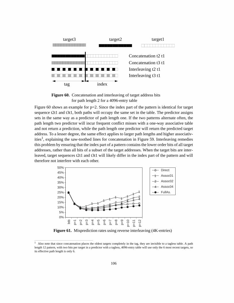
106

Figure 60 shows an example for p=2. Since the index part of the pattern is identical for targetsequence t2t1 and t3t1, both paths will occupy the same set in the table. The predictor assignssets in the same way as a predictor of path length one. If the two patterns alternate often, thepath length two predictor will incur frequent conflict misses with a one-way associative tableand not return a prediction, while the path length one predictor will return the predicted targetaddress. To a lesser degree, the same effect applies to larger path lengths and higher associativ-ities1, explaining the saw-toothed lines for concatenation in Figure 59. Interleaving remediesthis problem by ensuring that the index part of a pattern contains the lower order bits of all targetaddresses, rather than all bits of a subset of the target addresses. When the target bits are inter-leaved, target sequences t2t1 and t3t1 will likely differ in the index part of the pattern and willtherefore not interfere with each other.

1 Also note that since concatenation places the oldest targets completely in the tag, they are invisible to a tagless table. A pathlength 12 pattern, with two bits per target in a predictor with a tagless, 4096-entry table will use only the 6 most recent targets, soits effective path length is only 6.

target2 target1

Concatenation t2 t1

indextag

Interleaving t3 t1

Figure 60. Concatenation and interleaving of target address bits

target3

Concatenation t3 t1

Interleaving t2 t1

for path length 2 for a 4096-entry table

Figure 61. Misprediction rates using reverse interleaving (4K-entries)

0

00 0 0 0 0 0 0 0 0 0 0

1

11 1

1 11 1

1 11

112

22 2 2 2 2 2

2 22

2 24

44 4 4 4 4 4 4 4

4 4 4

btb

p=1

p=2

p=3

p=4

p=5

p=6

p=7

p=8

p=9

p=10

p=11

p=12

0%

5%

10%

15%

20%

25%

30%

35%

40%

45%

50%0 Direct

1 Assoc01

2 Assoc02

4 Assoc04

FullAs.

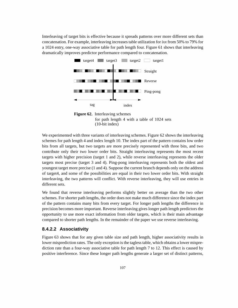
107

Interleaving of target bits is effective because it spreads patterns over more different sets thanconcatenation. For example, interleaving increases table utilization forixx from 50% to 79% fora 1024 entry, one-way associative table for path length four. Figure 61 shows that interleavingdramatically improves predictor performance compared to concatenation.

We experimented with three variants of interleaving schemes. Figure 62 shows the interleavingschemes for path length 4 and index length 10. The index part of the pattern contains low orderbits from all targets, but two targets are more precisely represented with three bits, and twocontribute only their two lower order bits. Straight interleaving represents the most recenttargets with higher precision (target 1 and 2), while reverse interleaving represents the oldertargets most precise (target 3 and 4). Ping-pong interleaving represents both the oldest andyoungest target more precise (1 and 4). Suppose the current branch depends only on the addressof target4, and some of the possibilities are equal in their two lower order bits. With straightinterleaving, the two patterns will conflict. With reverse interleaving, they will use entries indifferent sets.

We found that reverse interleaving performs slightly better on average than the two otherschemes. For shorter path lengths, the order does not make much difference since the index partof the pattern contains many bits from every target. For longer path lengths the difference inprecision becomes more important. Reverse interleaving gives longer path length predictors theopportunity to use more exact information from older targets, which is their main advantagecompared to shorter path lengths. In the remainder of the paper we use reverse interleaving.

8.4.2.2 Associativity

Figure 63 shows that for any given table size and path length, higher associativity results inlower misprediction rates. The only exception is the tagless table, which obtains a lower mispre-diction rate than a four-way associative table for path length 7 to 12. This effect is caused bypositive interference. Since these longer path lengths generate a larger set of distinct patterns,

Figure 62. Interleaving schemes

Straight

indextag

target3target4

Reverse

Ping-pong

target1target2

for path length 4 with a table of 1024 sets(10-bit index)

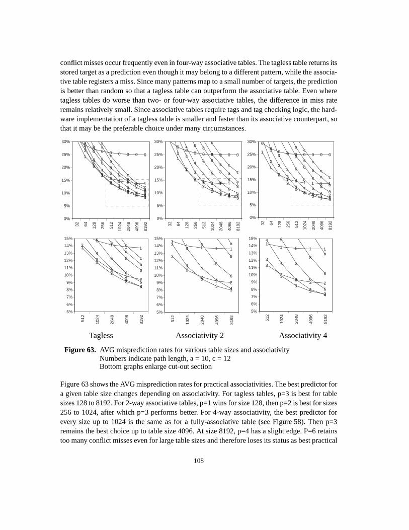
108

conflict misses occur frequently even in four-way associative tables. The tagless table returns itsstored target as a prediction even though it may belong to a different pattern, while the associa-tive table registers a miss. Since many patterns map to a small number of targets, the predictionis better than random so that a tagless table can outperform the associative table. Even wheretagless tables do worse than two- or four-way associative tables, the difference in miss rateremains relatively small. Since associative tables require tags and tag checking logic, the hard-ware implementation of a tagless table is smaller and faster than its associative counterpart, sothat it may be the preferable choice under many circumstances.

Figure 63 shows the AVG misprediction rates for practical associativities. The best predictor fora given table size changes depending on associativity. For tagless tables, p=3 is best for tablesizes 128 to 8192. For 2-way associative tables, p=1 wins for size 128, then p=2 is best for sizes256 to 1024, after which p=3 performs better. For 4-way associativity, the best predictor forevery size up to 1024 is the same as for a fully-associative table (see Figure 58). Then p=3remains the best choice up to table size 4096. At size 8192, p=4 has a slight edge. P=6 retainstoo many conflict misses even for large table sizes and therefore loses its status as best practical

00 0 0 0 0 0 01

1

11

1 1 1 1

2

2

2

22

2 2 2

3

3

3

33

33 3

4

4

4

4

44

4 4

6

6

6

6

66

6

8

8

8

8

88

8

a

a

a

aa

a

c

c

c

c

cc

32 64 128

256

512

1024

2048

4096

8192

0%

5%

10%

15%

20%

25%

30%0

00 0 0 0 0 0

1

1

11 1 1 1 1

2

2

2

22

2 2 2

3

3

3

33 3 3

4

4

4

4

44

4

6

6

6

6

66

8

8

8

8

8

a

a

a

a

c

c

c

c32 64 128

256

512

1024

2048

4096

8192

0%

5%

10%

15%

20%

25%

30% 00

0 0 0 0 0 0 01

1

11 1 1 1 1 1

2

2

22

2 2 2 2

3

3

3

33

3 3 3

4

4

4

44

4 4

6

6

6

66

6

8

8

8

88

a

a

a

a

a

c

c

c

c

32 64 128

256

512

1024

2048

4096

8192

0%

5%

10%

15%

20%

25%

30%

11 1 1 1

2

2

22 2

3

3

3

33

4

4

4

4

6

6

6

8

a

512

1024

2048

4096

8192

5%

6%

7%

8%

9%

10%

11%

12%

13%

14%

15%11 1 1

2

2

22

2

3

3

3

33

4

4

4

4

6

6

6

6

8

8

8

a

a

c

c

512

1024

2048

4096

8192

5%

6%

7%

8%

9%

10%

11%

12%

13%

14%

15%1

1 1 1 1

2

22

2 2

3

3

33

3

4

4

4

44

6

6

6

6

8

8

a

512

1024

2048

4096

8192

5%

6%

7%

8%

9%

10%

11%

12%

13%

14%

15%

Tagless Associativity 2 Associativity 4

Figure 63. AVG misprediction rates for various table sizes and associativityNumbers indicate path length, a = 10, c = 12Bottom graphs enlarge cut-out section

109

predictor. Limited table size and associativity prevent the predictor from taking full advantageof the longer-term regularity detection capability of longer path length predictors (however, seethe next section). Table A-1 in the appendix shows the exact misprediction rates for the bestpredictors for all table sizes, and Table A-2 contains their path lengths.

8.5 Summary

We have explored a wide range of two-level indirect branch predictors, starting with uncon-strained predictors with full-precision addresses and unlimited hardware resources. For a suiteof large C++ and C programs totalling more than half a million lines of source code, the bestunconstrained predictor achieved a misprediction rate of 5.8%, indicating that indirect branchesare intrinsically predictable even though current hardware predictors (BTBs) do not predictthem well. An exhaustive search of the design space established that a global history and per-address predictors perform best.

Subsequent experiments introduced resource constraints in order to evaluate whether realisticpredictors could approach this performance with a limited hardware budget. Introducinglimited-precision addresses (for a history buffer of 24 bits) increased the misprediction rate to6.0%. Limiting table size (thus causing capacity misses) resulted in a further increase to a 8.5%misprediction rate for a 1K-entry table and 6.6% for a 8K-entry table. Restricting table associa-tivity resulted in 11.7% and 8.5% misprediction rates for 1K and 8K tagless tables, respectively.Four-way associative tables of the same sizes reduce the misprediction rates to 9.8% and 7.3%,respectively. In comparison, an infinite-size fully-associative branch target buffer achieves abest-case misprediction rate of 24.9%. In other words, two-level prediction improves predictionaccuracy by more than a factor three.

We also explored a variety of alternatives that resulted in inferior performance. In particular:

• Per-address or per-set history buffers perform worse than a global, shared history buffer.

• Updating targets on every miss lowers the performance, compared to updating only aftertwo consecutive misses.

• Including conditional branch targets in the history pattern lowers prediction performanceby pushing the more relevant indirect branch information out of the history buffer.

• Using bits other than the lower-order bits of target addresses results in lower performance.

• For limited-associative tables, the index part of the key pattern should contain bits from asmany targets as possible, i.e., interleaving of target address bits performs better thanconcatenation.

The difference in performance between a BTB and the best practical two-level predictorbecomes significant only for history tables larger than 64 entries. As the hardware budget allowslarger history tables to be implemented, the path length of the best predictor grows.

110

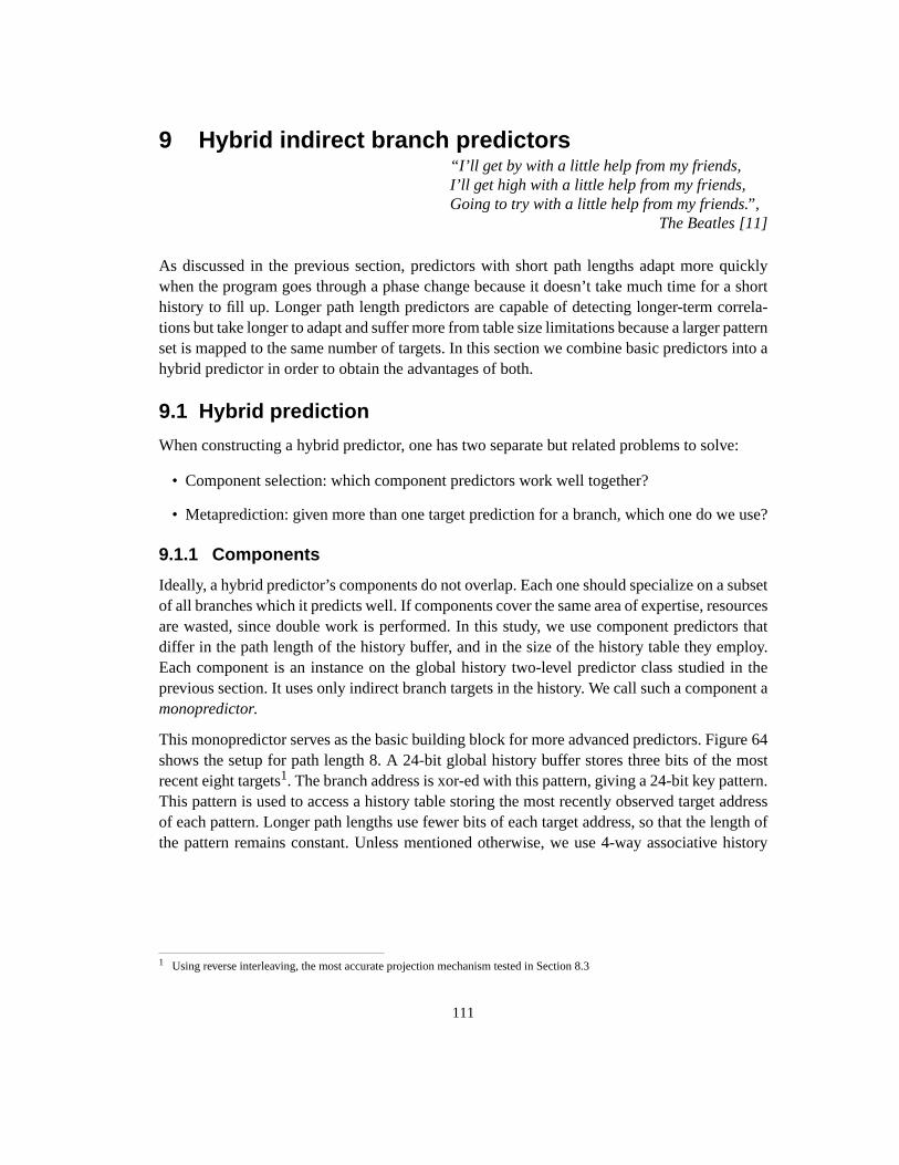
111

9 Hybrid indirect branch predictors“I’ll get by with a little help from my friends,I’ll get high with a little help from my friends,Going to try with a little help from my friends.”,

The Beatles [11]

As discussed in the previous section, predictors with short path lengths adapt more quicklywhen the program goes through a phase change because it doesn’t take much time for a shorthistory to fill up. Longer path length predictors are capable of detecting longer-term correla-tions but take longer to adapt and suffer more from table size limitations because a larger patternset is mapped to the same number of targets. In this section we combine basic predictors into ahybrid predictor in order to obtain the advantages of both.

9.1 Hybrid prediction

When constructing a hybrid predictor, one has two separate but related problems to solve:

• Component selection: which component predictors work well together?

• Metaprediction: given more than one target prediction for a branch, which one do we use?

9.1.1 Components

Ideally, a hybrid predictor’s components do not overlap. Each one should specialize on a subsetof all branches which it predicts well. If components cover the same area of expertise, resourcesare wasted, since double work is performed. In this study, we use component predictors thatdiffer in the path length of the history buffer, and in the size of the history table they employ.Each component is an instance on the global history two-level predictor class studied in theprevious section. It uses only indirect branch targets in the history. We call such a component amonopredictor.

This monopredictor serves as the basic building block for more advanced predictors. Figure 64shows the setup for path length 8. A 24-bit global history buffer stores three bits of the mostrecent eight targets1. The branch address is xor-ed with this pattern, giving a 24-bit key pattern.This pattern is used to access a history table storing the most recently observed target addressof each pattern. Longer path lengths use fewer bits of each target address, so that the length ofthe pattern remains constant. Unless mentioned otherwise, we use 4-way associative history

1 Using reverse interleaving, the most accurate projection mechanism tested in Section 8.3

112

tables1, and table entries are updated only after two consecutive mispredictions. We will referto this setup as amonopredictorof path length p.

9.1.2 Meta prediction

A hybrid branch predictor combines two or more component predictors that each predict atarget for the current branch. The hybrid predictor therefore needs a selection mechanism topredict which of the predictors is likely to be most accurate. We call this prediction of predictionaccuracymetaprediction. In the literature, at least two metaprediction mechanism are explored.A Branch Predictor Selection Table (BPST), proposed my McFarling [98], associates a two-bitcounter with each branch to keep track which of two component predictors is more accurate.After resolving a branch, the counter is updated to reflect the relative accuracy of the twocomponents. Alternatively, branches can be partitioned into different classes based on run-timeor compile-time information, and each class is associated with the component predictor bestsuited to handle it, as proposed by Chang, Hao and Patt [23].

The hybrid predictors presented in this chapter differ mainly by their meta prediction technique.Component predictor path lengths are tuned by varying their separate path lengths until theprediction accuracy, averaged over the benchmark suite (AVG), is maximized.

1 We show tags in figures only where they are required for correct operation of the predictor, as in the cascaded predictor. However,in the simulations we measure all setups with 4-way associative (tagged) tables in order to remove the noise of extensive conflictmisses.

Branch Address

History Table

XOR

History Buffer

8 recent targets3 lower order bits per target

Pattern projector for path length 8

Figure 64. Basic component predictor.

24 bit key pattern

For each path length between 0 and 12, the pattern projector constructs a keyof 24 bits, which is then used to access a history table that stores targetaddresses.

113

9.2 Branch classification

A classifying hybrid predictor, first explored by Chang, Hao and Patt [23] for conditionalbranch prediction, assigns to each branch a branch class. All branches that belong to a class usethe same component predictor. Classification therefore implements a kind of off-line metapre-diction. Before the program is run, it is determined for each branch which component deliversa target prediction. This means that only one component executes for every branch, allowingcomponents to share resources such as a prediction table.

In our experiments, component predictors differ only by global history path length. While everycomponent predictor’s history pattern is updated by all branches, only one is selected forprediction based on the branch class. The classifying predictor can use a shared history table forall component predictors (as shown in Figure 65) or several separate tables.

First, we study classification based on a branch’s source-level origin (indirect call, virtual call,or switch statement). Then we classify branches based on the number of different targetsencountered in a program run (thearity of a branch).

9.2.1 Opcode-based classification

In a first experiment, we classified branches into three classes: switch, virtual call, and indirectcall. The GNU compiler translates switch statements with more than seven cases into an indi-rect jump; no other C/C++ constructs use an indirect jump1, and thus this class is easy to recog-nize. To recognizevirtual function calls, we used EEL [89] to look for the characteristic five-instruction sequence generated by gcc and marked the corresponding call instruction accord-

1 They use jump and link (JMPL) instead of jump (JMP), in order to return to the call point.

Branch Address

History Table

Branch ClassBranch Target

Class1 History

Class2 History

Class3 History

BranchClass?

XOR

Key pattern

Figure 65. Classifying hybrid predictor with shared history table

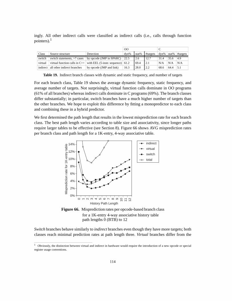
114

ingly. All other indirect calls were classified as indirect calls (i.e., calls through functionpointers).1

For each branch class, Table 19 shows the average dynamic frequency, static frequency, andaverage number of targets. Not surprisingly, virtual function calls dominate in OO programs(61% of all branches) whereas indirect calls dominate in C programs (69%). The branch classesdiffer substantially; in particular, switch branches have a much higher number of targets thanthe other branches. We hope to exploit this difference by fitting a monopredictor to each classand combining these in a hybrid predictor.

We first determined the path length that results in the lowest misprediction rate for each branchclass. The best path length varies according to table size and associativity, since longer pathsrequire larger tables to be effective (see Section 8). Figure 66 shows AVG misprediction ratesper branch class and path length for a 1K-entry, 4-way associative table.

Switch branches behave similarly toindirect branches even though they have more targets; bothclasses reach minimal prediction rates at path length three.Virtual branches differ from the

1 Obviously, the distinction between virtual and indirect in hardware would require the introduction of a new opcode or specialregister usage conventions.

OO C

Class Source structure Detection dyn% stat% #targets dyn% stat% #targets

switch switch statements, >7 cases by opcode (JMP in SPARC) 22.5 2.6 12.7 31.4 35.6 4.9

virtual virtual function calls in C++ with EEL (5-instr. sequence) 61.2 69.4 2.1 N/A N/A N/A

indirect all other indirect branches by opcode (JMP and link) 16.3 28.0 2.2 68.6 64.4 5.1

Table 19. Indirect branch classes with dynamic and static frequency, and number of targets0 1 2 3 4 5 6 7 8 9 10 11 12

0%

2%

4%

6%

8%

10%

12%

14%

Mis

pred

ictio

n ra

te fo

r 1K

-ent

ry ta

ble

History Path Length

indirect

virtual

switch

total

Figure 66. Misprediction rates per opcode-based branch classfor a 1K-entry 4-way associative history tablepath lengths 0 (BTB) to 12

115

other classes in that their ideal path length is slightly shorter, i.e. they correlate with morerecently executed branches.

After finding the best path length for each branch class separately, we calculated the mispredic-tion rate of a classifying predictor using separate tables for each class. For a given total tablesize T, one of the component predictors uses a table of T/2 entries, the other two componentsuse T/4 entries1. From the three possible configurations we selected the one with the lowestmiss rate. We then used the best path lengths for separate component predictors of size T, 2Tand 4T, to run a simulation of a shared-table classifying predictor of size T.

Table 20 and Figure 67 show the resulting predictor performances in comparison with a non-classifying monopredictor of equal size. Path lengths for the indirect and switch branch classare nearly identical over all table sizes. Virtual branches are better predicted by shorter pathlengths.

Clearly, classifying predictors with separate tables don’t perform well, having uniformly highermisprediction rates than a monopredictors. These predictors do not utilize their table space effi-ciently since the relative frequency of the different branch classes varies widely across bench-marks. For instance, C programs do not have virtual branches, so at least a quarter of the totaltable space is unused. A shared-table classifying predictor performs better, obtaining auniformly lower misprediction rate than a monopredictor of equivalent size. This result demon-strates that per-class path length determination does pay off, although the gain is quite small sothat the higher hardware cost of opcode-based prediction does not seem justified.

1 In these and later experiments, the total number of table entries is a power of two, in order to make point-to-point comparisonswith two-level monopredictors.

64 128

256

512

1024

2048

4096

8192

1638

4

0%

5%

10%

15%

20%

25%

30%

Mis

pred

ictio

n ra

te

Table size

Separate

Shared

Mono

Figure 67. Misprediction rates for opcode-based classifying predictors

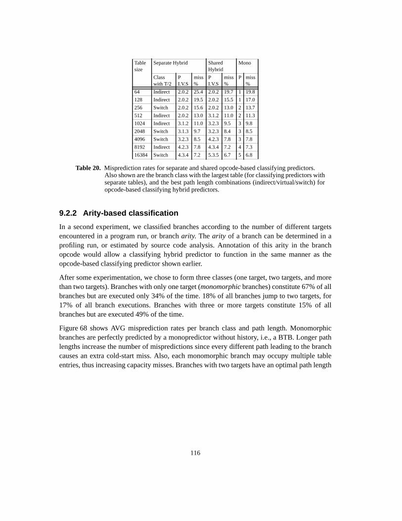
116

9.2.2 Arity-based classification

In a second experiment, we classified branches according to the number of different targetsencountered in a program run, or brancharity. Thearity of a branch can be determined in aprofiling run, or estimated by source code analysis. Annotation of this arity in the branchopcode would allow a classifying hybrid predictor to function in the same manner as theopcode-based classifying predictor shown earlier.

After some experimentation, we chose to form three classes (one target, two targets, and morethan two targets). Branches with only one target (monomorphic branches) constitute 67% of allbranches but are executed only 34% of the time. 18% of all branches jump to two targets, for17% of all branch executions. Branches with three or more targets constitute 15% of allbranches but are executed 49% of the time.

Figure 68 shows AVG misprediction rates per branch class and path length. Monomorphicbranches are perfectly predicted by a monopredictor without history, i.e., a BTB. Longer pathlengths increase the number of mispredictions since every different path leading to the branchcauses an extra cold-start miss. Also, each monomorphic branch may occupy multiple tableentries, thus increasing capacity misses. Branches with two targets have an optimal path length

Tablesize

Separate Hybrid SharedHybrid

Mono

Classwith T/2

PI.V.S

miss%

PI.V.S

miss%

P miss%

64 Indirect 2.0.2 25.4 2.0.2 19.7 1 19.8

128 Indirect 2.0.2 19.5 2.0.2 15.5 1 17.0

256 Switch 2.0.2 15.6 2.0.2 13.0 2 13.7

512 Indirect 2.0.2 13.0 3.1.2 11.0 2 11.3

1024 Indirect 3.1.2 11.0 3.2.3 9.5 3 9.8

2048 Switch 3.1.3 9.7 3.2.3 8.4 3 8.5

4096 Switch 3.2.3 8.5 4.2.3 7.8 3 7.8

8192 Indirect 4.2.3 7.8 4.3.4 7.2 4 7.3

16384 Switch 4.3.4 7.2 5.3.5 6.7 5 6.8

Table 20. Misprediction rates for separate and shared opcode-based classifying predictors.Also shown are the branch class with the largest table (for classifying predictors withseparate tables), and the best path length combinations (indirect/virtual/switch) foropcode-based classifying hybrid predictors.

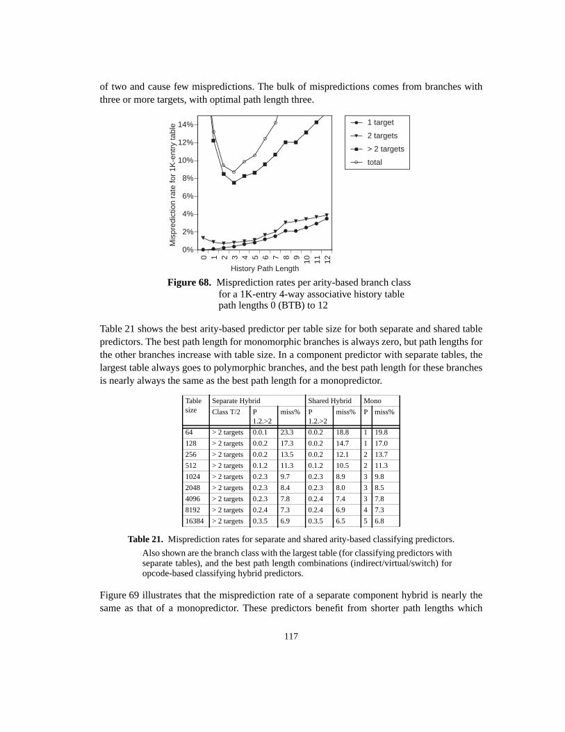
117

of two and cause few mispredictions. The bulk of mispredictions comes from branches withthree or more targets, with optimal path length three.

Table 21 shows the best arity-based predictor per table size for both separate and shared tablepredictors. The best path length for monomorphic branches is always zero, but path lengths forthe other branches increase with table size. In a component predictor with separate tables, thelargest table always goes to polymorphic branches, and the best path length for these branchesis nearly always the same as the best path length for a monopredictor.

Figure 69 illustrates that the misprediction rate of a separate component hybrid is nearly thesame as that of a monopredictor. These predictors benefit from shorter path lengths which

Tablesize

Separate Hybrid Shared Hybrid Mono

Class T/2 P1.2.>2

miss% P1.2.>2

miss% P miss%

64 > 2 targets 0.0.1 23.3 0.0.2 18.8 1 19.8

128 > 2 targets 0.0.2 17.3 0.0.2 14.7 1 17.0

256 > 2 targets 0.0.2 13.5 0.0.2 12.1 2 13.7

512 > 2 targets 0.1.2 11.3 0.1.2 10.5 2 11.3

1024 > 2 targets 0.2.3 9.7 0.2.3 8.9 3 9.8

2048 > 2 targets 0.2.3 8.4 0.2.3 8.0 3 8.5

4096 > 2 targets 0.2.3 7.8 0.2.4 7.4 3 7.8

8192 > 2 targets 0.2.4 7.3 0.2.4 6.9 4 7.3

16384 > 2 targets 0.3.5 6.9 0.3.5 6.5 5 6.8

Table 21. Misprediction rates for separate and shared arity-based classifying predictors.

Figure 68. Misprediction rates per arity-based branch class

0 1 2 3 4 5 6 7 8 9 10 11 12

0%

2%

4%

6%

8%

10%

12%

14%

Mis

pred

ictio

n ra

te fo

r 1K

-ent

ry ta

ble

History Path Length

1 target

2 targets

> 2 targets

total

for a 1K-entry 4-way associative history tablepath lengths 0 (BTB) to 12

Also shown are the branch class with the largest table (for classifying predictors withseparate tables), and the best path length combinations (indirect/virtual/switch) foropcode-based classifying hybrid predictors.

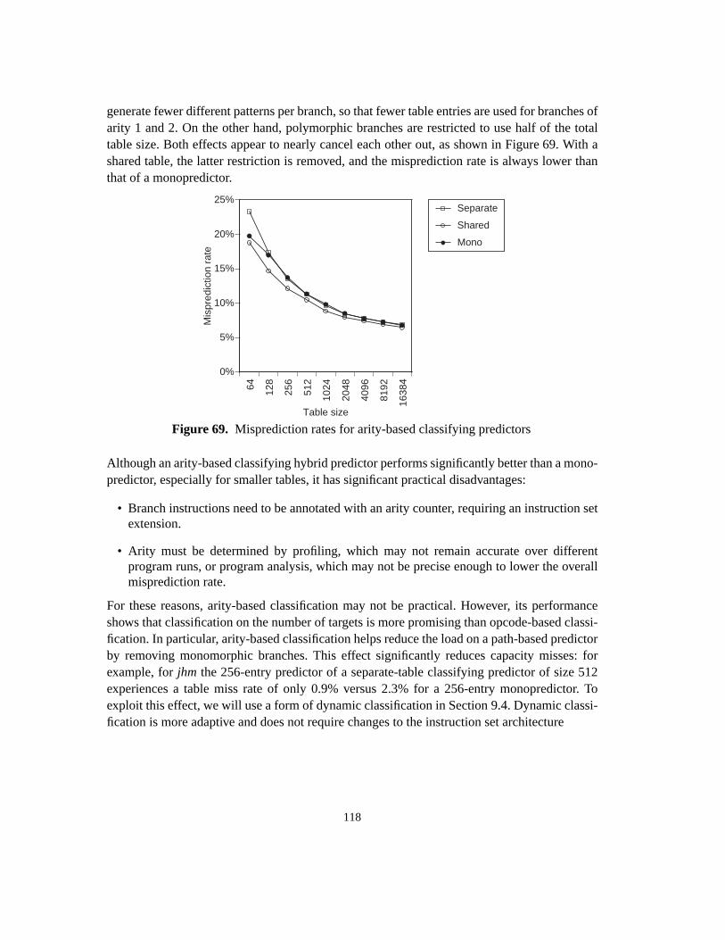
118

generate fewer different patterns per branch, so that fewer table entries are used for branches ofarity 1 and 2. On the other hand, polymorphic branches are restricted to use half of the totaltable size. Both effects appear to nearly cancel each other out, as shown in Figure 69. With ashared table, the latter restriction is removed, and the misprediction rate is always lower thanthat of a monopredictor.

Although an arity-based classifying hybrid predictor performs significantly better than a mono-predictor, especially for smaller tables, it has significant practical disadvantages:

• Branch instructions need to be annotated with an arity counter, requiring an instruction setextension.

• Arity must be determined by profiling, which may not remain accurate over differentprogram runs, or program analysis, which may not be precise enough to lower the overallmisprediction rate.

For these reasons, arity-based classification may not be practical. However, its performanceshows that classification on the number of targets is more promising than opcode-based classi-fication. In particular, arity-based classification helps reduce the load on a path-based predictorby removing monomorphic branches. This effect significantly reduces capacity misses: forexample, forjhm the 256-entry predictor of a separate-table classifying predictor of size 512experiences a table miss rate of only 0.9% versus 2.3% for a 256-entry monopredictor. Toexploit this effect, we will use a form of dynamic classification in Section 9.4. Dynamic classi-fication is more adaptive and does not require changes to the instruction set architecture

64 128

256

512

1024

2048

4096

8192

1638

4

0%

5%

10%

15%

20%

25%M

ispr

edic

tion

rate

Table size

Separate

Shared

Mono

Figure 69. Misprediction rates for arity-based classifying predictors

119

9.2.3 Discussion

Classifying predictors match branches to predictor components in a round-about way: first thebranch is assigned to a class, and then a predictor component is tuned (by varying path length)to a branch class. Much depends on the uniformity of branches within a class. If classes are toocoarsely defined, as in the opcode classification experiment, then there is no class-specificbehavior to take advantage of. In the arity-based classification experiment, the per-classbehavior is much more distinct, allowing a closer match between a branch and a predictorcomponent. However, some branches may still be misclassified. A duomorphic branch mayjump to the same target most of the time1, and could therefore benefit from classification intothe monomorphic class. The classification mechanism could take this into account by classi-fying branches according to the number of times they undergo a target change. Many such alter-native classification criteria can be conceived. However, a branch whose behavior (and thus itsclassification) varies according to program input, will be misclassified in some program runs.Ideally, a branch should be classified according to its current behavior, i.e. if the behavior variesbetween program runs or between program phases in the same run, then the branch should bere-classified. Dynamic classification at run time can deliver more accurate metaprediction (andthus prediction), because it uses more up to date information.

In the next section, we cut out the classification step and match a branch directly to a compo-nent, based on its run-time behavior.

1 For instance, if it tests for exceptions or end conditions in a loop

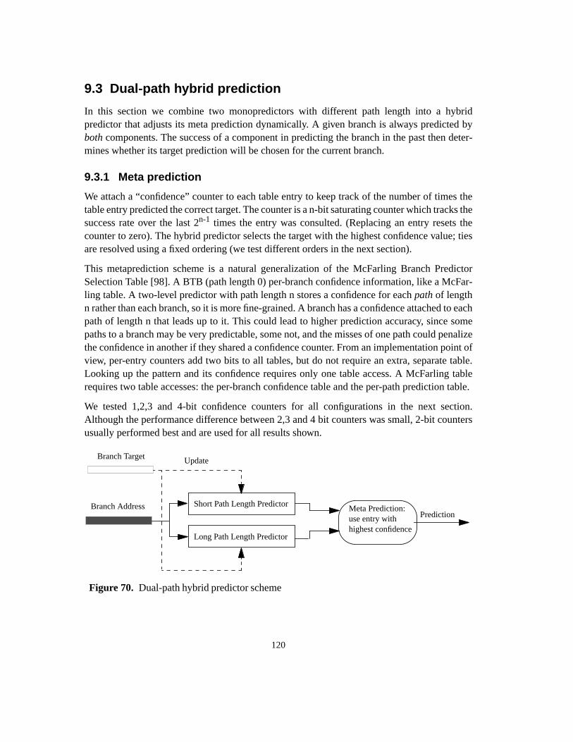
120

9.3 Dual-path hybrid prediction

In this section we combine two monopredictors with different path length into a hybridpredictor that adjusts its meta prediction dynamically. A given branch is always predicted byboth components. The success of a component in predicting the branch in the past then deter-mines whether its target prediction will be chosen for the current branch.

9.3.1 Meta prediction

We attach a “confidence” counter to each table entry to keep track of the number of times thetable entry predicted the correct target. The counter is a n-bit saturating counter which tracks thesuccess rate over the last 2n-1 times the entry was consulted. (Replacing an entry resets thecounter to zero). The hybrid predictor selects the target with the highest confidence value; tiesare resolved using a fixed ordering (we test different orders in the next section).

This metaprediction scheme is a natural generalization of the McFarling Branch PredictorSelection Table [98]. A BTB (path length 0) per-branch confidence information, like a McFar-ling table. A two-level predictor with path length n stores a confidence for eachpath of lengthn rather than each branch, so it is more fine-grained. A branch has a confidence attached to eachpath of length n that leads up to it. This could lead to higher prediction accuracy, since somepaths to a branch may be very predictable, some not, and the misses of one path could penalizethe confidence in another if they shared a confidence counter. From an implementation point ofview, per-entry counters add two bits to all tables, but do not require an extra, separate table.Looking up the pattern and its confidence requires only one table access. A McFarling tablerequires two table accesses: the per-branch confidence table and the per-path prediction table.

We tested 1,2,3 and 4-bit confidence counters for all configurations in the next section.Although the performance difference between 2,3 and 4 bit counters was small, 2-bit countersusually performed best and are used for all results shown.

Figure 70. Dual-path hybrid predictor scheme

Branch Address Short Path Length Predictor

Long Path Length Predictor

Branch Target Update

PredictionMeta Prediction:use entry withhighest confidence

121

9.3.2 Component predictors

We simulate hybrid predictors with two component predictors of equal table size and associa-tivity but different path lengths1. The component table sizes vary from 32 entries to 16K entries,and we simulate all combinations of path lengths in the range 0..12.

Figure 71 shows the AVG hit ratios for two component table sizes with representative behavior(2048 and 8192); more details are given in Table 22. The best hit rates are obtained by thecombination of a short path length predictor (p=1..3) with a longer path length predictor(p=5..12). Since the curve is fairly symmetrical with respect to the diagonal, it appears that theorder of the predictors (which is used to break ties in component predictor selection) does notmatter much. For smaller tables, the curve is sharper and peaks at shorter path lengths, i.e., it thechoice of the short path length component is more important, and very short path lengths domuch better.

1 Chronologically, this study was performed before the branch classification study. Therefore we still test different associativities.As this section shows, a hybrid predictor suffers from conflict misses to the same extent as its component predictors do. In laterstudies we only consider 4-way associative tables in order to remove most of the noise of conflict misses, and to cut down on thenumber of different configurations to be run through our simulation engine.

Figure 71. Prediction hit rates for dual-path hybrid predictors, all path length combinations.

01

23

45

P1 67

89

1011

12

01

23

45 P26

78

910

1112

95%94%93%92%91%90%

95%94%93%92%91%90%

01

23

45

P1 67

89

1011

12

01

23

45 P26

78

910

1112

95%94%93%92%91%90%

95%94%93%92%91%90%

4-way associative tables with 2-bit confidence counters and component table size of2048(left) and 8192(right) entries. P1 is the path length of the first component predictor,P2 of the second. When P1 = P2 (the diagonal), the hit rate for a non-hybrid predictor oftwice the component size is shown.

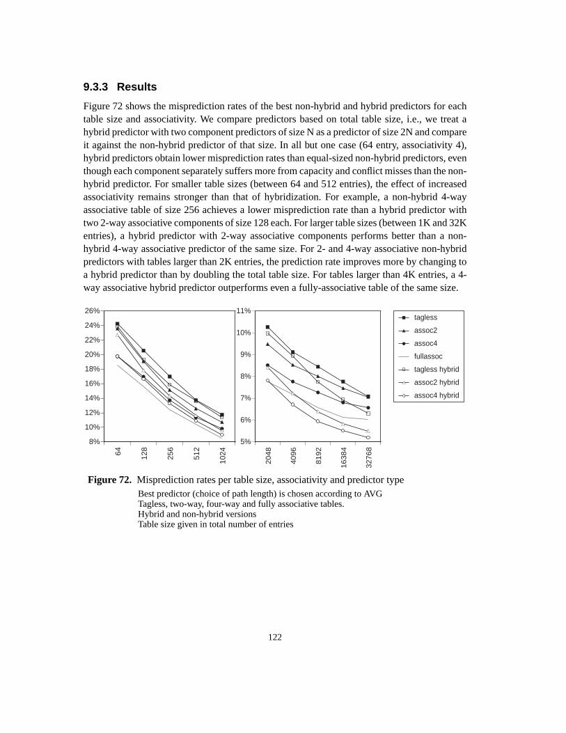
122

9.3.3 Results

Figure 72 shows the misprediction rates of the best non-hybrid and hybrid predictors for eachtable size and associativity. We compare predictors based on total table size, i.e., we treat ahybrid predictor with two component predictors of size N as a predictor of size 2N and compareit against the non-hybrid predictor of that size. In all but one case (64 entry, associativity 4),hybrid predictors obtain lower misprediction rates than equal-sized non-hybrid predictors, eventhough each component separately suffers more from capacity and conflict misses than the non-hybrid predictor. For smaller table sizes (between 64 and 512 entries), the effect of increasedassociativity remains stronger than that of hybridization. For example, a non-hybrid 4-wayassociative table of size 256 achieves a lower misprediction rate than a hybrid predictor withtwo 2-way associative components of size 128 each. For larger table sizes (between 1K and 32Kentries), a hybrid predictor with 2-way associative components performs better than a non-hybrid 4-way associative predictor of the same size. For 2- and 4-way associative non-hybridpredictors with tables larger than 2K entries, the prediction rate improves more by changing toa hybrid predictor than by doubling the total table size. For tables larger than 4K entries, a 4-way associative hybrid predictor outperforms even a fully-associative table of the same size.

Figure 72. Misprediction rates per table size, associativity and predictor type

64 128

256

512

1024

8%

10%

12%

14%

16%

18%

20%

22%

24%

26%

2048

4096

8192

16384

32768

5%

6%

7%

8%

9%

10%

11%tagless

assoc2

assoc4

fullassoc

tagless hybrid

assoc2 hybrid

assoc4 hybrid

Best predictor (choice of path length) is chosen according to AVGTagless, two-way, four-way and fully associative tables.Hybrid and non-hybrid versionsTable size given in total number of entries

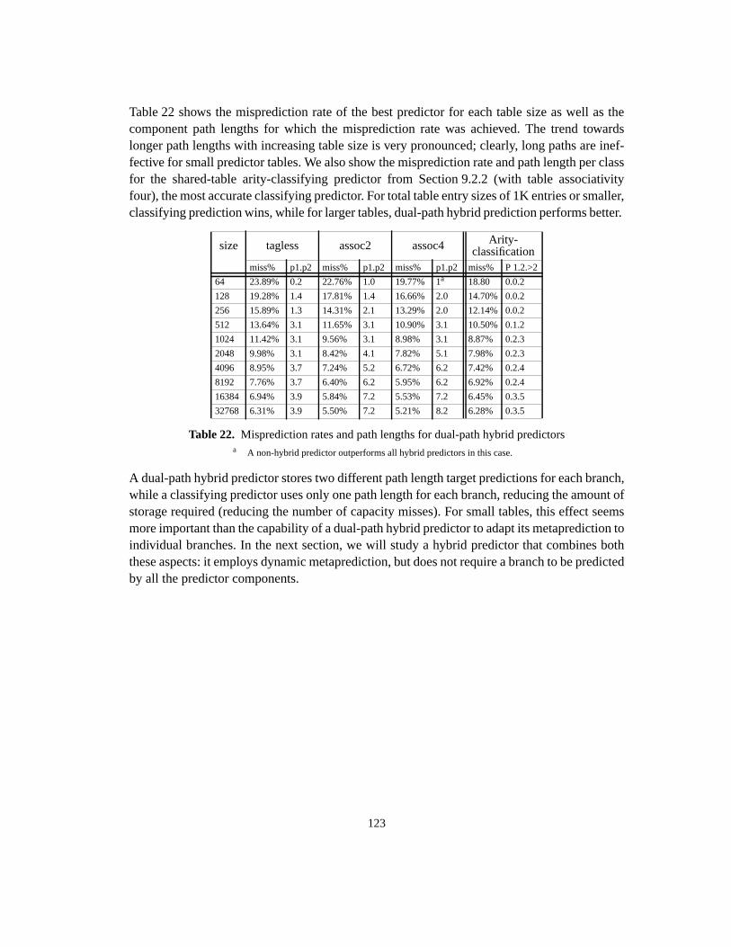
123

Table 22 shows the misprediction rate of the best predictor for each table size as well as thecomponent path lengths for which the misprediction rate was achieved. The trend towardslonger path lengths with increasing table size is very pronounced; clearly, long paths are inef-fective for small predictor tables. We also show the misprediction rate and path length per classfor the shared-table arity-classifying predictor from Section 9.2.2 (with table associativityfour), the most accurate classifying predictor. For total table entry sizes of 1K entries or smaller,classifying prediction wins, while for larger tables, dual-path hybrid prediction performs better.

A dual-path hybrid predictor stores two different path length target predictions for each branch,while a classifying predictor uses only one path length for each branch, reducing the amount ofstorage required (reducing the number of capacity misses). For small tables, this effect seemsmore important than the capability of a dual-path hybrid predictor to adapt its metaprediction toindividual branches. In the next section, we will study a hybrid predictor that combines boththese aspects: it employs dynamic metaprediction, but does not require a branch to be predictedby all the predictor components.

a A non-hybrid predictor outperforms all hybrid predictors in this case.

size tagless assoc2 assoc4 Arity-classification

miss% p1.p2 miss% p1.p2 miss% p1.p2 miss% P 1.2.>2

64 23.89% 0.2 22.76% 1.0 19.77% 1a 18.80 0.0.2

128 19.28% 1.4 17.81% 1.4 16.66% 2.0 14.70% 0.0.2

256 15.89% 1.3 14.31% 2.1 13.29% 2.0 12.14% 0.0.2

512 13.64% 3.1 11.65% 3.1 10.90% 3.1 10.50% 0.1.2

1024 11.42% 3.1 9.56% 3.1 8.98% 3.1 8.87% 0.2.3

2048 9.98% 3.1 8.42% 4.1 7.82% 5.1 7.98% 0.2.3

4096 8.95% 3.7 7.24% 5.2 6.72% 6.2 7.42% 0.2.4

8192 7.76% 3.7 6.40% 6.2 5.95% 6.2 6.92% 0.2.4

16384 6.94% 3.9 5.84% 7.2 5.53% 7.2 6.45% 0.3.5

32768 6.31% 3.9 5.50% 7.2 5.21% 8.2 6.28% 0.3.5

Table 22. Misprediction rates and path lengths for dual-path hybrid predictors

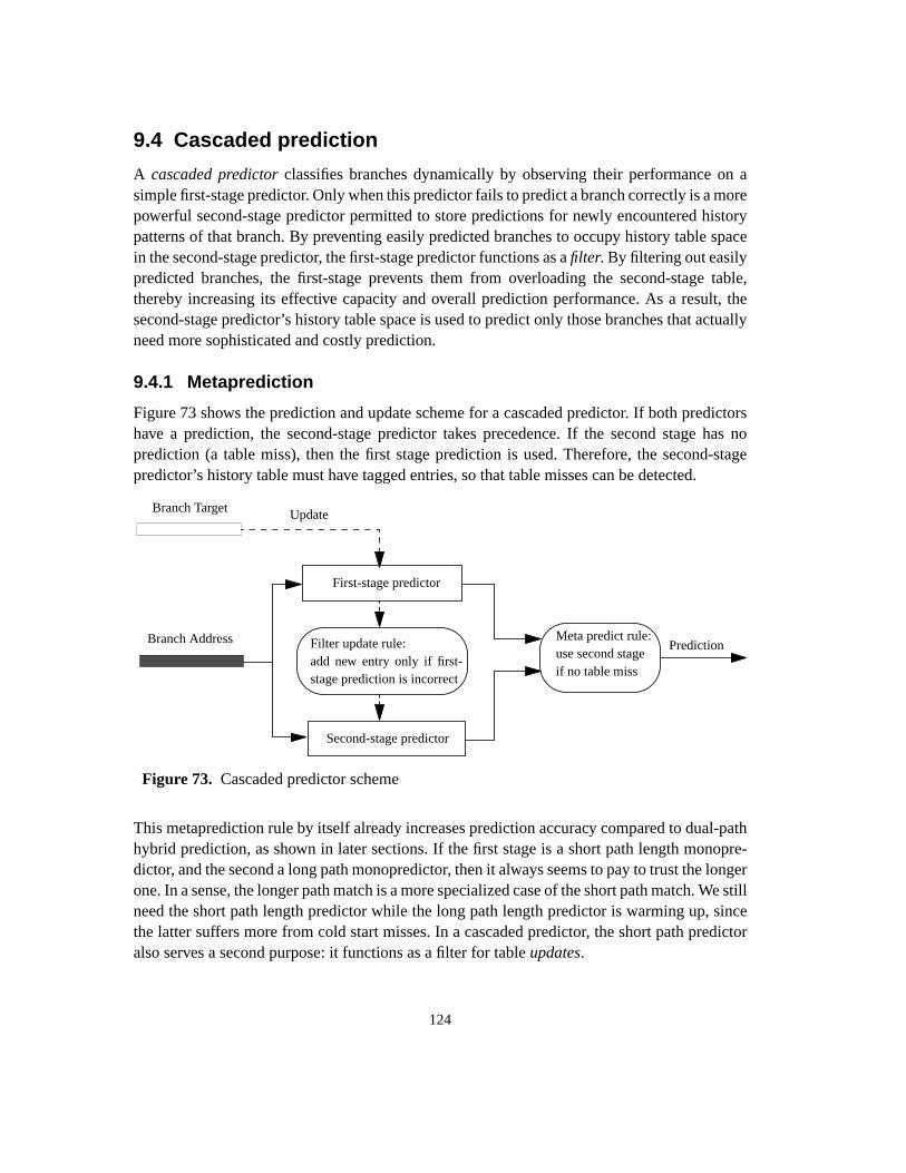
124

9.4 Cascaded prediction

A cascaded predictor classifies branches dynamically by observing their performance on asimple first-stage predictor. Only when this predictor fails to predict a branch correctly is a morepowerful second-stage predictor permitted to store predictions for newly encountered historypatterns of that branch. By preventing easily predicted branches to occupy history table spacein the second-stage predictor, the first-stage predictor functions as afilter. By filtering out easilypredicted branches, the first-stage prevents them from overloading the second-stage table,thereby increasing its effective capacity and overall prediction performance. As a result, thesecond-stage predictor’s history table space is used to predict only those branches that actuallyneed more sophisticated and costly prediction.

9.4.1 Metaprediction

Figure 73 shows the prediction and update scheme for a cascaded predictor. If both predictorshave a prediction, the second-stage predictor takes precedence. If the second stage has noprediction (a table miss), then the first stage prediction is used. Therefore, the second-stagepredictor’s history table must have tagged entries, so that table misses can be detected.

This metaprediction rule by itself already increases prediction accuracy compared to dual-pathhybrid prediction, as shown in later sections. If the first stage is a short path length monopre-dictor, and the second a long path monopredictor, then it always seems to pay to trust the longerone. In a sense, the longer path match is a more specialized case of the short path match. We stillneed the short path length predictor while the long path length predictor is warming up, sincethe latter suffers more from cold start misses. In a cascaded predictor, the short path predictoralso serves a second purpose: it functions as a filter for tableupdates.

Filter update rule:add new entry only if first-stage prediction is incorrect

Branch Address

First-stage predictor

Second-stage predictor

Branch Target Update

Figure 73. Cascaded predictor scheme

PredictionMeta predict rule:use second stageif no table miss

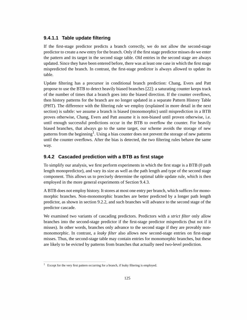
125

9.4.1.1 Table update filtering

If the first-stage predictor predicts a branch correctly, we do not allow the second-stagepredictor to create anew entry for the branch. Only if the first stage predictor misses do we enterthe pattern and its target in the second stage table. Old entries in the second stage are alwaysupdated. Since they have been entered before, there was at least one case in which the first stagemispredicted the branch. In contrast, the first-stage predictor is always allowed to update itstable.

Update filtering has a precursor in conditional branch prediction: Chang, Evers and Pattpropose to use the BTB to detect heavily biased branches [22]: a saturating counter keeps trackof the number of times that a branch goes into the biased direction. If the counter overflows,then history patterns for the branch are no longer updated in a separate Pattern History Table(PHT). The difference with the filtering rule we employ (explained in more detail in the nextsection) is subtle: we assume a branch is biased (monomorphic) until misprediction in a BTBproves otherwise, Chang, Evers and Patt assume it is non-biased until proven otherwise, i.e.until enough successful predictions occur in the BTB to overflow the counter. For heavilybiased branches, that always go to the same target, our scheme avoids the storage of newpatterns from the beginning1. Using a bias counter does not prevent the storage of new patternsuntil the counter overflows. After the bias is detected, the two filtering rules behave the sameway.

9.4.2 Cascaded prediction with a BTB as first stage

To simplify our analysis, we first perform experiments in which the first stage is a BTB (0 pathlength monopredictor), and vary its size as well as the path length and type of the second stagecomponent. This allows us to precisely determine the optimal table update rule, which is thenemployed in the more general experiments of Section 9.4.3.

A BTB does not employ history. It stores at most one entry per branch, which suffices for mono-morphic branches. Non-monomorphic branches are better predicted by a longer path lengthpredictor, as shown in section 9.2.2, and such branches will advance to the second stage of thepredictor cascade.

We examined two variants of cascading predictors. Predictors with astrict filter only allowbranches into the second-stage predictor if the first-stage predictor mispredicts (but not if itmisses). In other words, branches only advance to the second stage if they are provably non-monomorphic. In contrast, aleaky filter also allows new second-stage entries on first-stagemisses. Thus, the second-stage table may contain entries for monomorphic branches, but theseare likely to be evicted by patterns from branches that actually need two-level prediction.

1 Except for the very first pattern occurring for a branch, if leaky filtering is employed.

126

9.4.2.1 Strict filters

Successful prediction in the filter classifies a branch as monomorphic (if only temporarily). Ifa branch misses in the filter predictor, nothing conclusive is known: every branch incurs acompulsory table miss in the filter, even if it is purely monomorphic. To prevent cold-startmisses of the filter to pass through to the second-stage predictor, strict filtering disallows newentry insertion in the second-stage predictor on a miss (but not on a mispredict). To implementthis strict filter design, the filter’s table must be tagged.

Figure 74 shows the misprediction rates for three selected second-stage predictors (each withoptimal path length for its size). We also show the misprediction rate of a cascaded predictorwithout filtering. Even without filtering, the first-stage predictor reduces overall mispredictionrates compared to the stand-alone predictor (shown as filter size 0) by providing an educatedguess in the case of a table miss in the second-stage predictor. In other words, a cascadedpredictor consisting of a BTB and a path-based predictor reduces cold-start misses even withoutfiltering. We call this astaged predictor (see Section 9.4.3)

Strict filters do not perform well for small filter table sizes. For 16 entries or less, overallmisprediction rates are even higher than that of the stand-alone predictor. Essentially, a strictfilter predictor recognizes branches as polymorphic only if the branch remains in the filter tablelong enough to incur a target change (and thus a misprediction). But with small filters, manypolymorphic branches are displaced from the filter before they mispredict, and thus they neverenter the second stage. When the filter becomes large enough to avoid most capacity misses,this effect disappears and filtering starts to pay off. At 256 entries, strict filtering performs as

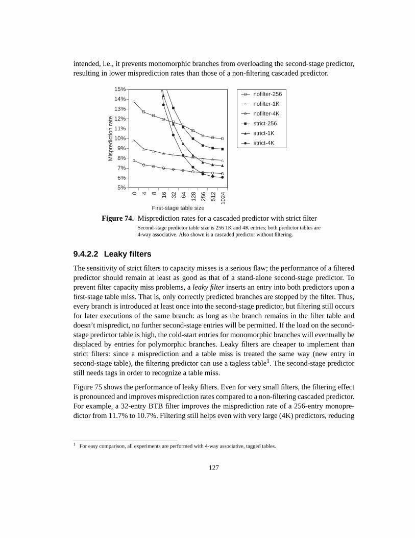
127

intended, i.e., it prevents monomorphic branches from overloading the second-stage predictor,resulting in lower misprediction rates than those of a non-filtering cascaded predictor.

9.4.2.2 Leaky filters

The sensitivity of strict filters to capacity misses is a serious flaw; the performance of a filteredpredictor should remain at least as good as that of a stand-alone second-stage predictor. Toprevent filter capacity miss problems, aleaky filter inserts an entry into both predictors upon afirst-stage table miss. That is, only correctly predicted branches are stopped by the filter. Thus,every branch is introduced at least once into the second-stage predictor, but filtering still occursfor later executions of the same branch: as long as the branch remains in the filter table anddoesn’t mispredict, no further second-stage entries will be permitted. If the load on the second-stage predictor table is high, the cold-start entries for monomorphic branches will eventually bedisplaced by entries for polymorphic branches. Leaky filters are cheaper to implement thanstrict filters: since a misprediction and a table miss is treated the same way (new entry insecond-stage table), the filtering predictor can use a tagless table1. The second-stage predictorstill needs tags in order to recognize a table miss.

Figure 75 shows the performance of leaky filters. Even for very small filters, the filtering effectis pronounced and improves misprediction rates compared to a non-filtering cascaded predictor.For example, a 32-entry BTB filter improves the misprediction rate of a 256-entry monopre-dictor from 11.7% to 10.7%. Filtering still helps even with very large (4K) predictors, reducing

1 For easy comparison, all experiments are performed with 4-way associative, tagged tables.

0 4 8 16 32 64 128

256

512

1024

5%

6%

7%

8%

9%

10%

11%

12%

13%

14%

15%

Mis

pred

ictio

n ra

te

First-stage table size

nofilter-256

nofilter-1K

nofilter-4K

strict-256

strict-1K

strict-4K

Figure 74. Misprediction rates for a cascaded predictor with strict filterSecond-stage predictor table size is 256 1K and 4K entries; both predictor tables are4-way associative. Also shown is a cascaded predictor without filtering.

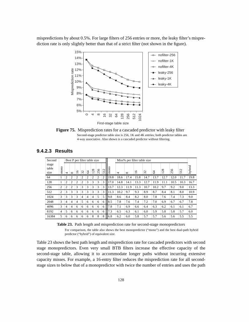
128

mispredictions by about 0.5%. For large filters of 256 entries or more, the leaky filter’s mispre-diction rate is only slightly better than that of a strict filter (not shown in the figure).

9.4.2.3 Results

Table 23 shows the best path length and misprediction rate for cascaded predictors with secondstage monopredictors. Even very small BTB filters increase the effective capacity of thesecond-stage table, allowing it to accommodate longer paths without incurring extensivecapacity misses. For example, a 16-entry filter reduces the misprediction rate for all second-stage sizes to below that of a monopredictor with twice the number of entries and uses the path

Secondstagetablesize m

ono

Best P per filter table size

mon

o

Miss% per filter table size

hybr

id

4 8 16 32 64 128

256

512

4 8 16 32 64 128

256

512

64 1 2 2 2 2 2 2 2 2 19.8 18.6 17.4 15.8 14.7 13.7 12.7 12.0 11.7 19.8

128 1 2 2 2 2 3 3 3 3 17.0 14.8 14.1 13.3 12.7 11.9 11.1 10.5 10.3 16.7

256 2 2 2 3 3 3 3 3 3 13.7 12.3 11.9 11.3 10.7 10.2 9.7 9.2 9.0 13.3

512 2 3 3 3 3 3 3 3 3 11.3 10.2 9.7 9.3 8.9 8.7 8.4 8.1 8.0 10.9

1024 3 3 3 3 4 4 4 5 5 9.8 8.6 8.4 8.2 8.0 7.8 7.6 7.4 7.3 9.0

2048 3 4 4 4 5 6 6 6 6 8.5 7.8 7.6 7.4 7.2 7.0 6.9 6.7 6.7 7.8

4096 3 4 4 6 6 6 6 6 6 7.8 7.1 6.9 6.6 6.4 6.3 6.2 6.1 6.1 6.7

8192 4 5 6 6 6 6 6 6 6 7.3 6.5 6.3 6.1 6.0 5.9 5.8 5.8 5.7 6.0

16384 5 6 6 6 6 6 8 8 8 6.8 6.2 6.0 5.8 5.7 5.7 5.6 5.6 5.5 5.5

Table 23. Path length and misprediction rate for second-stage monopredictors

0 4 8 16 32 64 128

256

512

1024

5%

6%

7%

8%

9%

10%

11%

12%

13%

14%

15%

Mis

pred

ictio

n ra

te

First-stage table size

nofilter-256

nofilter-1K

nofilter-4K

leaky-256

leaky-1K

leaky-4K

Figure 75. Misprediction rates for a cascaded predictor with leaky filterSecond-stage predictor table size is 256, 1K and 4K entries; both predictor tables are4-way associative. Also shown is a cascaded predictor without filtering.

For comparison, the table also shows the best monopredictor (“mono”) and the best dual-path hybridpredictor (“hybrid”) of equivalent size.

129

length of a monopredictor that is four times larger. A 64-entry filter lowers the mispredictionrate below that of a monopredictor four times as large, and for all table sizes smaller than 1Kentries, beyond that of a dual-path hybrid predictor of twice the size.

We also studied cascaded predictors that use dual-path hybrid predictors in the second stage,anticipating that filtering would again reduce second-stage misses and allow longer pathlengths. For each filtered hybrid of table size T, we simulated the best path length couples ofnon-cascaded dual-path hybrid predictors of section 9.3 with table sizes T, 2T and 4T.

The resulting improvements were equally pronounced (Table 24). Again, filtering reduces themisprediction rate and increases the best path length choices for each table size. Whereas non-cascaded predictors need at least 1024 table entries to achieve misprediction rates below 9%, afiltered dual-path hybrid attains this threshold with only 544 entries (32-entry filter BTB plus512-entry dual-path hybrid). Adding an 8-entry filter to a 1K-entry hybrid predictor lowers itsmisprediction rate from 9.0% to 8.2%. A 128-entry filter reduces this to 7.5%. Across all tablesizes, cascaded prediction reduces table size by roughly a factor of two.

Secondleveltablesize hy

brid

Best P per filter table size

hybr

id

Miss% per filter table size

4 8 16 32 64 128

256

512

4 8 16 32 64 128

256

512

64 1.1 2.0 2.0 2.0 2.0 2.0 2.0 2.0 2.0 19.8 20.6 19.3 18.3 17.5 15.8 14.7 13.9 13.6

128 2.0 2.0 3.1 3.1 3.1 3.1 3.1 3.1 3.1 16.7 15.5 14.9 13.9 13.1 12.4 11.4 10.7 10.4

256 2.0 3.1 3.1 3.1 3.1 3.1 3.1 3.1 3.1 13.3 12.3 11.8 11.3 10.9 10.5 9.9 9.3 9.1

512 3.1 3.1 5.1 5.1 5.1 5.1 5.1 5.1 5.1 10.9 10.0 9.6 9.3 9.0 8.8 8.5 8.1 8.0

1024 3.1 5.1 5.1 6.2 6.2 6.2 6.2 6.2 6.2 9.0 8.2 8.0 7.7 7.5 7.3 7.1 6.9 6.8

2048 5.1 6.2 6.2 6.2 6.2 6.2 6.2 6.2 6.2 7.8 7.1 6.9 6.7 6.5 6.5 6.4 6.3 6.2

4096 6.2 6.2 7.2 7.2 7.2 7.2 7.2 7.2 7.2 6.7 6.3 6.1 6.0 5.9 5.9 5.8 5.8 5.7

8192 6.2 8.2 8.2 8.2 8.2 8.2 8.2 8.2 8.2 6.0 5.6 5.5 5.5 5.4 5.4 5.4 5.3 5.3

16384 7.2 8.2 8.2 8.2 8.2 8.2 8.2 8.2 8.2 5.5 5.3 5.2 5.2 5.2 5.1 5.1 5.1 5.1

Table 24. Path length and misprediction rate for second-stage dual-path hybrid predictors

For comparison, the table also shows the best the best dual-path hybrid predictor (“hybrid”) ofequivalent size.

130

Figure 76 shows AVG misprediction rates for selected prediction schemes. For all schemes andtable sizes, filtering reduces misprediction rates. For tables of 512 entries or less, the resultingmisprediction rate of filtered monopredictors is equal or lower than that of filtered dual-pathhybrid predictors. This is due to a filter’s cold-start miss reduction (it usually has a zero pathlength prediction if the second stage has not yet encountered the longer path). A dual-pathhybrid predictor does not get extra benefit from this effect at small table sizes, since its shortercomponent’s path length is already close or equal to zero. Most of the misprediction rate reduc-tion of small hybrid predictors is therefore due solely to the filter’s capacity miss reduction.Mono predictors, with path lengths of two or three, benefit both from capacity miss reductionand cold-start miss reduction. The resulting misprediction rates end up being fairly similar formono and hybrid predictors. However, for second-stage tables of 1K entries and larger, thefiltered hybrid predictor’s misprediction rate is substantially lower than that of a filtered mono-predictor at all filter sizes. Since the short component path length is two in most of these cases,a filter’s cold-start miss reduction also benefits a dual-path length hybrid predictor. At the highend of the table size range (+8K), conflict and capacity misses become less frequent, and thebenefit of filtering starts to diminish.

Figures 77,78 and 79 show misprediction rates for the self, edg andgcc benchmarks1. Theformer two programs have the largest number of active branches in the benchmark suite. Thereduction in misprediction rate is higher than the reductions on AVG of Figure 76, which showsthat the benefit of filtering is especially pronounced for large programs.

1 Best mono predictor path lengths are determined separately for each benchmark. Hybrid predictor path lengths are picked fromthe AVG path length choices.

64 128

256

512

1024

6%

8%

10%

12%

14%

16%

18%

20%M

ispr

edic

tion

rate

Table size

1024

2048

4096

8192

1638

4

5%

6%

7%

8%

9%

10%

Mis

pred

ictio

n ra

teTable size

mono

8/mono

128/mono

hybrid

8/hybrid

128/hybrid

Figure 76. AVG misprediction rates without filters and with 8 and 128-entry filters.Second stage predictors are mono and dual-path length hybrid predictorsWe use different scales for small and large table sizes to increase visibility.

131

1024

2048

4096

8192

1638

4

8%

9%

10%

11%

12%

13%

14%

15%

16%

17%

18%

Mis

pred

ictio

n ra

te

Table size

mono

8/mono

128/mono

hybrid

8/hybrid

128/hybrid

Figure 77. Self misprediction rates without filters and with 8 and 128-entry filters

64 128

256

512

1024

10%

15%

20%

25%

30%

35%

40%

Mis

pred

ictio

n ra

te

Table size

64 128

256

512

1024

10%

15%

20%

25%

30%

35%

Mis

pred

ictio

n ra

te

Table size

1024

2048

4096

8192

1638

47%

8%

9%

10%

11%

12%

13%

14%

15%M

ispr

edic

tion

rate

Table size

mono

8/mono

128/mono

hybrid

8/hybrid

128/hybrid

Figure 78. Edg misprediction rates without filters and with 8 and 128-entry filters

64 128

256

512

1024

15%

20%

25%

30%

35%

40%

45%

Mis

pred

ictio

n ra

te

Table size

1024

2048

4096

8192

1638

4

10%11%12%13%14%15%16%17%18%19%20%21%22%23%24%

Mis

pred

ictio

n ra

te

Table size

mono

8/mono

128/mono

hybrid

8/hybrid

128/hybrid

Figure 79. Gcc misprediction rates without filters and with 8 and 128-entry filters

132

9.4.3 Multi-stage cascaded prediction

In the previous section we determined the optimal metaprediction and update filtering rule fora cascaded predictor, on the simplified case where the first stage predictor is a history-less (0path length) BTB. Here we investigate the accuracy of a natural generalization of this two-stagepredictor by allowing any type of predictor in the first stage and any number of stages. First, weuse the maximum number of stages, and unlimited, fully associative tables for each stage, todetermine the limit of prediction accuracy reachable by this architecture. Then we test two andthree stage predictors for a wide range of table sizes, to investigate how close we can get to thelimit with a practical architecture.

9.4.3.1 Predictor components

Figure 80 shows representative examples of the predictors used in this study. The simplestarchitecture is abranch target buffer (BTB). A selection of bits from the branch address servesas a key pattern into a predictor table, which stores the last target observed for this branch.

A two-level predictor extends the BTB scheme by taking bits from the last p branch targetspreceding the execution of the current branch and xor-ing these bits with the branch address.The parameter p is thepath length of the two-level predictor.

A cascaded predictor consists of several stages, each containing a two-level predictor with itsown history buffer and predictor table. Successive stages use increasing path lengths (in prelim-inary experiments we observed the consistently inferior accuracy of decreasing path lengths).The use of separate tables allows all stages to predict in parallel. In a final step, the predictorchooses the prediction from the last stage that did not encounter a table miss. This ensures thatits target prediction is based on the longest available path history.

A cascaded predictor saves table space by using aleaky filter update rule (see Section 9.4.2): anew history pattern enters a long path length stage only if none of the shorter stages predictedthe branch correctly. This rule prevents easily predicted branches from occupying table space inan expensive, long path length stage. For example, branches with only a single target areperfectly predicted by a BTB, after the initial compulsory miss, so they do not need a longhistory pattern. As a result, the longer path length stage encounters fewer capacity misses,improving overall prediction accuracy.

We also measure the accuracy of a cascaded predictor without filtering. We call this astagedpredictor. Staged predictors, even without filtering, improve prediction accuracy compared to atwo-level predictor because they reduce cold start misses. Longer path length two-level predic-tors are more accurate than short path length predictors, but they need a longer time to reach thatpotential since they store more patterns per branch. In a staged predictor, the early stages predictmany branches accurately while the later stages are warming up. This also reduces theeffect ofcapacity misses in later stages, since an earlier stage is likely to have a (less accurate) predictionavailable in the case of a late stage capacity miss.

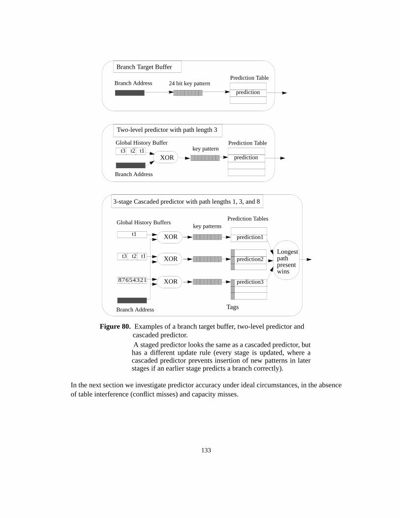
133

In the next section we investigate predictor accuracy under ideal circumstances, in the absenceof table interference (conflict misses) and capacity misses.

Branch Address

Figure 80. Examples of a branch target buffer, two-level predictor andcascaded predictor.

24 bit key pattern

Branch Target Buffer

Branch Address

Prediction Table

XOR

Global History Bufferkey pattern

prediction

Two-level predictor with path length 3

Branch Address

Prediction Tables

XOR

Global History Bufferskey patterns

t1 prediction1

3-stage Cascaded predictor with path lengths 1, 3, and 8

XORt1t2t3 prediction2

XOR1 prediction32345678

Longestpathpresentwins

t1t2t3

Prediction Table

prediction

Tags

A staged predictor looks the same as a cascaded predictor, buthas a different update rule (every stage is updated, where acascaded predictor prevents insertion of new patterns in laterstages if an earlier stage predicts a branch correctly).

134

9.4.3.2 Ideal predictors

We use the termideal for a predictor scheme with an unlimited, fully associative predictor table.The misprediction rate measured for such a predictor is free from the noise of conflict andcapacity misses. This allows us to compare the intrinsic strength of different predictionschemes, and provides us with a limit beyond which prediction cannot be improved merely byspending more transistors on predictor tables.

In one respect, the predictors studied in this section are not ideal: they have limited 24-bithistory buffers. History buffers must be kept small because they determine the cost of a tableentry through the size of the tag. A small buffer represents each target with few bits, and this cancause pattern interference, reducing prediction accuracy. However, a 24-bit history buffersuffices for near-ideal accuracy. Beyond path length 12, a 24-bit history buffer causes extensivepattern interference because it stores only one bit for some targets. Therefore we do not use pathlengths longer than 12. This restriction does not substantially reduce the potential accuracy, aswe found during a preliminary experiment with a 30-bit buffer and path lengths up to 15.

Ideal cascaded predictors have a full complement of stages. For example, an ideal cascadedpredictor of path length 6 has 7 stages, consisting of ideal two-level predictors with path lengths0 (a BTB) up to 6. Similarly, and idealstaged predictor also has the maximum number of stages,but does not employ pattern filtering.

Figure 81 shows misprediction rates for ideal two-level predictors, cascaded predictors andstaged predictors for path lengths from 0 to 12. Two-level prediction reaches a minimummisprediction rate of 6.0% at path length 6. Longer path lengths show increasing mispredictionrates, because cold start misses start to negate the advantage of capturing longer-term correla-tions. The loss of accuracy due to pattern interference is small, as shown by the accuracy of anideal two-level predictor with unlimited buffer size (see Section 8). Where path lengths areinteger factors of the buffer size, enabling full buffer use, interference is negligible (path lengths0 to 4, 6, 8 and 12). Only for path lengths that use less than the full history buffer does themisprediction rate increase noticeably. For example, path length 9 in a 24 -bit history bufferuses only two bits per target, for a total of 18 bits1. The difference in accuracy, represented by

Terminology Description

Unlimited ideal two-level ofpath length P

Two-level predictor with an unlimited history buffer, storing a concatena-tion of full precision addresses of the P most recent targets, with an unlim-ited, fully associative predictor table

Ideal two-level of path length PTwo-level predictor with 24-bit history buffer, storing the xor of (24 div P)bits of the P most recent targets, with an unlimited, fully associative predic-tor table

Ideal branch target buffer (BTB) Ideal two-level predictor of path length 0

Ideal staged of path length P A non-filtering staged predictor, with P+1 stages, consisting of ideal two-level predictors of path length 0,1,..,P

Ideal cascaded of path length P An ideal staged predictor of path length P, with filtering of new patterns

Table 25. Ideal predictor terminology

135

the “bump” in the curves, is strictly due to pattern interference. The curves for cascaded predic-tion and staged prediction show similar bumps, the most prominent at path length 9.

An ideal cascaded predictor is better than ideal two-level prediction at all path lengths. Theshort path length stages in a cascaded (and a staged) predictor immediately start predictingmany branches accurately while the later stages are warming up, as explained inSection 9.4.3.1. This gives it an advantage over a two-level predictor of the same path lengtheven in the absence of capacity misses.

Staged prediction reaches lower misprediction rates than cascaded prediction at all path lengths.This is to be expected, since a cascaded predictor uses filtering and therefore stores strictly lessinformation than a staged predictor. Cascaded prediction merely economizes on the number oftable entries required by staged prediction, and this has no beneficial effect for ideal predictorswith unlimited tables.There simply are no capacity misses to reduce.

However, the reduction of table entry cost is dramatic, as shown in Figure 82. The graph showsthe total number of table entries occupied in a two-level, cascaded and staged predictor. As thepath lengths grows, a staged predictor’s size grows exponentially, while a cascaded and two-level predictor show nearly linear growth. At path length 12, a staged predictor occupies173325 entries, five times as much as a cascaded predictor (34572) and a two-level predictor(34076). The curves of cascaded and two-level prediction overlap almost completely,suggesting some systematic effect.We currently can not explain this similarity, but suspect thatthe exact reason for the close resemblance is to be found in information theory. In terms of

1 It is of course possible to fill the unused bit space with bits from a strict subset of the target addresses. This opens up a varietyof choices as to which targets should be represented with 1 bit extra accuracy. In the reverse interleaved address projectionemployed, this choice is unclear. To simplify our analysis, we left these bits unused.

Figure 81. Ideal two-level, fully cascaded and fully staged predictor misprediction rates

0 1 2 3 4 5 6 7 8 9 10 11 12

0%

5%

10%

15%

20%

25%

Mis

pred

ictio

n ra

te fo

r id

eal t

able

History Path Length

3 4 5 6 7 8 9 10 11 12

4%

5%

6%

7%

8%

History Path Length

TwoLevel

nCascaded

nStaged

TwoLevUnlim

For path lengths 0 to 12 (cutout enlarged in right graph)

136

branch prediction schemes, it means that a two-level predictor table cost is in the same ball parkas a fully cascaded predictor. However, the latter eliminates cold start misses, while preservingthe capacity to capture longer term correlations. In the next section we measure these benefitsin the context of practical predictors.

9.4.3.3 Practical predictors

In this section we study practical cascaded predictor architectures with limited, 4-way associa-tive tables and a small number of stages. Our aim is to reduce the number of table entriesrequired to attain a given prediction accuracy. We also want to find out how close we can get tothe prediction accuracy of the hypothetical ideal predictors of the previous section.

9.4.3.3.1 Practical predictor tables

The main cost of predictor architectures lies in the amount of on-chip memory required to storepredictions. In the previous section we saw that the total number of patterns generated by anideal predictor grows as its path length increases. For example, a two-level predictor reaches aminimal misprediction rate of 5.8% at path length 6, by storing13210 pattern/target associations(averaged over the AVG benchmarks). Given a table entry size of about 60 bits (24-bit tag, 1-bitupdate counter, and 32-bit target address), the resulting data structure takes up about 800 K bitsof memory, barely within the capability of current processor technology. We want to reduce thismemory cost while keeping misprediction rates as low as possible.

Reducing the size of a predictor table generatescapacity misses: a pattern/target association,though it was stored, and would have correctly predicted the target of a branch, was evictedfrom the table by a pattern/target of a more recently executed branch. For smaller tables, thepath length must be shortened to prevent extensive capacity misses. However, shorter path

Figure 82. Number of patterns stored by an ideal two-level, cascaded and staged predictor

0 1 2 3 4 5 6 7 8 9 10 11 12

0

20000

40000

60000

80000

100000

120000

140000

160000

180000

Num

ber

of ta

ble

entr

ies

touc

hed

History Path Length

TwoLevIdeal

nCascIdeal

nStageIdeal

137

length predictors are less accurate. For every given table size, there is some path length whichforms the optimal compromise between these opposing effects. We use simulation to determinethis optimal path length, and the resulting misprediction rate, for table sizes from 32 to 32Kentries.

One further limitation is necessary to allow limited size predictor tables to be implemented insilicon: a limited associativity (see Section 9). We use tables with associativity four, as usual.

9.4.3.3.2 Practical multi-stage predictors

A staged predictor must split up a given total table entry budget and allocate some part of it toeach stage. Although it is conceivable to use one global predictor table for all stages, this wouldrequire an expensive multi-access table. Therefore each stage uses a separate single-accesstable. For a given total table entry budget, we have the option of using many stages with smalltables, or few stages with large tables. Which one is better?

For a cascaded predictor, there are two opposite effects at work. On the one hand, partitioningtable space over a large number of stages increases the likelihood that a benchmark’s workingset overloads the capacity of any given stage, resulting in extensive capacity misses. This alsoreduces the efficiency of pattern filtering, since only correct predictions prevent patterns fromoccupying space in later stages. On the other hand, a large number of stages allows filtering tooccur at a stage with a shorter path length, reducing the total number of patterns stored. For ourbenchmark suite, a small number of stages uses a given table entry budget more effectively thana full complement of stages. For example, a cascaded predictor with 9 stages, from path length0 up to 8, with 128 entries per stage (total budget of 1152 entries) achieves a misprediction rateof 7.7%, while a 2-stage cascaded predictor with 512 entries per stage (total budget of 1024),and path lengths 1 and 8, reaches 6.8%.

We therefore focus on predictors with a small number of stages. From an analysis point of view,their superior accuracy is a windfall, since a small number of stages substantially reduces thenumber of different path length combinations to be simulated1. For 2-stage predictors withoutfiltering (staged), we test all path length combinations P1P2, with 0 <= P1 < P2 <= 12, for eachtotal table entry budget that is a power of 2 between 32 and 32K entries. Each stage uses half ofthe total table size.

We also determine optimal path length combinations for cascaded predictors. For the 2-stagecascaded predictor, we test the same range of path lengths as for the 2-stage non-filteringpredictor. However, we also simulate table entry budgets halfway between powers of 2 (in orderto compare with 3-stage predictors with same-size stages). In that case, two third of the entriesis allocated to the last stage.

1 An truly exhaustive study would require simulation of approximately #stages ^ (#tablesizes * #historylengths). For the range oftable sizes, history lengths and number of stages explored in this study, this would lead to 15 ^ (10 * 15) ~= 2.6E176 differentcombinations, far too many to explore within the given time frame.

138

For the 3-stage predictor we test all path length combinations with 0 <= P1 < P2 < P3 <= 12,with P1 <= 4, and P2 <= 10, to reduce the number of combinations without removing goodcandidates. We simulate the same range of total table entry budgets as for the 2-stage cascadedpredictor by using stage sizes X+X+X and X+X+2X, with X equal to a power of 2. Table 26summarizes the terminology.

9.4.3.4 Results

Figure 83 shows misprediction rates that result from using the best path length combinations foreach predictor configuration. Exact numbers with path length combinations can be found inTable 28. For comparison we also show the misprediction rate of a BTB and the best ideal two-level, cascaded and staged predictors of the previous section (shown as dotted lines parallel tothe x-axis since table size is not a factor).

Cascaded predictors perform better than two-level predictors at all table sizes in the exploredrange. In other words, any given misprediction rate is bought at a much lower cost. For instance,a 3-stage predictor of size 512 outperforms a two-level predictor of size 2K. At a fairly modest

Terminology Description

Two-level of size T Two-level predictor with a 4-way associative predictor table of size T

2-staged of size T A non-filtering staged predictor, using 2 two-level predictors of size T/2

2-staged cascaded of size TA 2-staged predictor of size T, with pattern filtering. If T is not a power of 2, thestages have size T/3 and 2T/3

3-staged cascaded of size TA 3-staged predictor with pattern filtering, using 3 two-level predictors of sizeT/3. If T is a power of 2, the stages have size T/4,T/4, and T/2

Table 26. Practical predictor configurations (path length combinations are tuned to each size T)

Figure83. Misprediction rates for practical two-level, staged and cascaded predic-tors

32 48 64 96 128

192

256

384

512

768

1024

1536

2048

3072

4096

6144

8192

1228

816

384

2457

632

768

0%

5%

10%

15%

20%

25%

30%

Mis

pred

ictio

n ra

te fo

r bes

t pat

hlen

gth

Table entry size

BTB

TwoLevel

2Stage

2Cascaded

3Cascaded

TwoLevIdeal

nCascadIdeal

nStageIdeal

512

768

1024

1536

2048

3072

4096

6144

8192

1228

8

1638

4

2457

6

3276

8

4%

5%

6%

7%

8%

9%

Table entry size

139

budget of 1.5K entries, a 3-staged cascaded predictor attains the same misprediction rate as anideal two-level predictor with an unlimited table.

3-stage cascaded predictors consistently outperform 2-stage predictors, and 2-stage cascadedpredictors outperform 2-stage (non-filtering) predictors. For limited budgets, cascaded predic-tion wins over staged prediction because pattern filtering reduces capacity misses, allowing acascaded predictor to use longer path lengths for any given table size.

2-and 3-staged predictors seem to get asymptotically close to the accuracy of an ideal stagedpredictor for large, but still practical table budgets. A small number of stages clearly suffices toget almost arbitrarily close to ideal accuracy. A 3-stage cascaded predictor, at 4K table entriesand higher, even improves upon the accuracy of an ideal cascaded predictor with a full comple-ment of stages. This surprising result indicates that a small number of stages improves predic-tion accuracy. The label “ideal” for a fully staged cascaded predictor thus seems to be amisnomer. We are not entirely sure why this is the case. Filtering seems to be responsible for thereduced accuracy, since a non-filtering ideal staged predictor still outperforms all other predic-tors. A small number of stages does not filter out as many patterns, and therefore it may repre-sent an intermediate between these extremes, at large table budgets1, resulting in anintermediate misprediction rate.

Do 3-stage cascaded predictors form the best possible configuration for a limited budget? Wethink not. Dividing the table entry budget over 8 stages gives worse performance than a 2-stagecascaded predictor, as shown above, so the optimal number of stages may lie somewhere inbetween 3 and 8, most likely at the lower end. However, the benefit of extra stages is not likelyto improve performance by a large factor. The difference between 2 and 3 stage cascadedprediction is already fairly small, allowing a 3-stage predictor of size 3X to reach the same orbetter performance than a 2-stage predictor of size 4X, as soon as X is larger than 512. Theadded complexity of extra stages may not be worth the effort.

We did not show staged predictors in which stages differ in size by a large degree, although wedid simulate 2-and 3stage predictors with the later stage(s) as much as a factor 32 larger than theearlier one(s). The results indicate that predictors with a table budget spread out evenly among(a small number of) stages perform best. This effect is already noticeable for the 3-stage predic-tors shown here, since the curve in Figure 83 shows slight bumps for those configurations withtotal table budgets that are powers of two. In other words, a 3-stage predictor with stages of sizeX+X+X performs relatively better, in accuracy per table entry, than a 3-stage predictor withstage sizes X+X+2X.

1 Positive interference could also be responsible. However, the tables are tagged, so this can only be pattern interference.

140

9.4.3.5 Detailed data

Table 27 shows misprediction rates and occupied table entries for ideal predictors with unlim-ited tables, for various path lengths.

Table entries Misprediction rates

Pat

h le

ngth

BT

B

Twol

evel

Cas

cade

d

Sta

ged

BT

B

Twol

evel

Cas

cade

d

Sta

ged

Unl

imite

d Tw

olev

e

0 356 356 356 356 24.9 24.9 24.9 24.9 24.91 356 1195 1191 1551 24.9 13.1 13.1 13.1 13.12 356 2617 2495 4169 24.9 8.8 8.8 8.6 8.83 356 4477 4266 8645 24.9 7.1 7.0 6.7 7.14 356 6863 6469 15508 24.9 6.5 6.3 5.9 6.45 356 8838 8940 24346 24.9 6.3 5.9 5.4 5.96 356 12324 11838 36670 24.9 6.0 5.5 4.8 5.87 356 14379 14935 51048 24.9 6.2 5.4 4.8 5.88 356 18580 18430 69629 24.9 6.2 5.2 4.5 6.09 356 18160 21914 87788 24.9 7.2 5.5 5.5 6.210 356 23061 25770 110849 24.9 7.2 5.4 5.1 6.511 356 28400 30003 139249 24.9 7.3 5.3 4.8 6.912 356 34076 34572 173325 24.9 7.5 5.2 4.6 7.3

Table 27. Total number of entries and misprediction rates for ideal BTB, two-level, fully cascaded andfully staged predictors, and for an ideal two-level predictor with unlimited history buffer

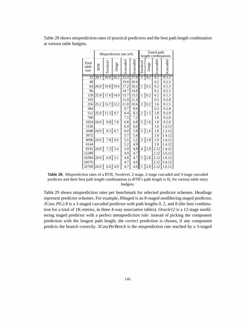
141

Table 28 shows misprediction rates of practical predictors and the best path length combinationat various table budgets.

Table 29 shows misprediction rates per benchmark for selected predictor schemes. Headingsrepresent predictor schemes. For example,8Staged is an 8-staged nonfiltering staged predictor,3Casc.P0.2.8 is a 3-staged cascaded predictor with path lengths 0, 2, and 8 (the best combina-tion for a total of 1K-entries, in three 4-way associative tables).Oracle12 is a 12-stage nonfil-tering staged predictor with a perfect metaprediction rule: instead of picking the componentprediction with the longest path length, thecorrect prediction is chosen, if any componentpredicts the branch correctly.3CascPerBench is the misprediction rate reached by a 3-staged

Misprediction rate in% Tuned pathlength combinations

Totaltablesize B

TB

Twol

evel

2sta

ge

2cas

cade

d

3cas

cade

d

Twol

evel

2sta

ge

2cas

cade

d

3cas

cade

d

32 28.1 26.0 26.2 22.4 27.6 1 0.2 0.2 0.1.248 19.0 20.6 0.2 0.2.364 26.8 19.8 19.6 17.2 18.2 1 0.2 0.2 0.1.396 14.7 14.8 0.2 0.2.5

128 25.8 17.0 14.9 13.7 13.5 1 0.2 0.2 0.1.3192 11.9 11.4 0.3 0.2.8256 25.1 13.7 12.2 11.0 10.6 2 0.2 1.6 0.1.5384 9.7 8.9 0.3 0.2.8512 25.0 11.3 9.7 8.4 8.3 2 1.5 1.8 0.2.8768 7.5 7.2 1.6 0.2.8

1024 24.9 9.8 7.8 6.8 6.8 3 1.6 1.8 0.2.81536 6.4 6.0 1.6 1.4.122048 24.9 8.5 6.7 6.0 5.8 3 1.6 1.8 1.3.123072 5.7 5.4 1.8 1.4.124096 24.9 7.8 6.0 5.5 5.2 3 2.8 1.8 1.4.126144 5.2 4.9 1.8 1.4.128192 24.9 7.3 5.4 5.0 4.8 4 2.8 2.12 1.4.12

12288 4.9 4.7 2.12 1.6.1216384 24.9 6.8 5.1 4.8 4.7 5 2.8 2.12 1.6.1224576 4.7 4.6 2.12 3.4.1232768 24.9 6.6 4.9 4.7 4.6 5 2.8 2.12 1.6.12

Table 28. Misprediction rates of a BTB, Twolevel, 2-stage, 2-stage cascaded and 3-stage cascadedpredictor and their best path length combinations (a BTB’s path length is 0), for various table entry

budgets.

142

cascaded predictor (1K-entry in this case), which is tuned specifically to each benchmark(instead of choosing path lengths which minimize AVG misprediction rates).

Namein

str.

/ ind

irect

cond

. / in

dire

ct

activebranches Ideal 1.5K 4-

way assoc 1K-4way assoc

99 %

100

%

Ora

cle1

2

8Sta

ged

8Cas

cade

d

P6T

woL

evel

Idea

l

BT

B

3Cas

c.P

1.4.

12

2Cas

c.P

1.6

3Cas

cPer

Ben

ch

3Cas

c.P

0.2.

8

2Cas

c.P

1.8

TwoL

evel

.P3

BT

B

idl 47 6 70 543 0.2 0.3 0.4 0.4 2.4 0.3 0.4 0.3 0.4 0.4 0.8 2.4jhm 47 5 34 155 2.1 8.1 8.6 8.7 11.1 8.7 9.7 8.6 9.9 9.6 11.3 11.1self 56 7 848 1855 3.1 7.4 8.0 10.1 15.7 12.2 12.9 12.2 12.4 13.9 18.6 16.3

xlisp 69 11 4 13 0.3 1.4 1.6 1.4 13.5 1.9 1.7 1.5 1.8 2.0 2.2 13.5troff 90 13 61 161 3.9 6.7 6.8 7.1 13.7 7.7 7.3 7.2 7.9 7.8 7.8 13.7lcom 97 10 87 328 0.4 0.8 0.9 1.4 4.2 1.2 1.2 1.3 1.3 1.4 2.2 4.2

AVG-100 68 9 184 509 1.7 4.1 4.4 4.8 10.1 5.3 5.5 5.2 5.6 5.9 7.2 10.2perl 113 17 7 24 0.2 0.2 0.2 0.5 31.8 0.2 0.2 0.2 0.2 0.2 0.3 31.8

porky 138 19 89 285 1.6 4.2 4.3 4.5 20.8 4.6 4.7 5.0 6.2 5.0 7.9 20.8ixx 139 18 91 203 1.5 3.5 4.0 5.6 45.7 3.3 4.5 3.3 4.2 4.0 9.0 45.7edg 149 23 186 350 3.4 7.2 8.1 11.9 35.9 8.9 9.6 9.4 9.6 9.4 16.3 35.9eqn 159 25 58 114 2.8 8.5 10.8 12.5 34.8 12.8 13.1 14.4 14.8 14.9 21.9 34.8gcc 176 31 95 166 2.6 8.2 11.9 11.7 65.7 14.8 15.1 15.3 17.3 17.2 23.6 65.7

beta 188 23 135 376 0.6 1.3 1.5 2.3 28.6 1.7 2.1 2.6 2.6 2.6 5.6 28.6AVG-200 152 22 94 217 1.8 4.7 5.8 7.0 37.6 6.6 7.1 7.2 7.8 7.6 12.1 37.6AVG 113 16 136 352 1.7 4.5 5.2 6.0 24.9 6.0 6.4 6.3 6.8 6.8 9.8 25.0AVG-OO 107 14 164 447 1.8 4.5 5.0 5.8 19.7 5.8 6.2 6.1 6.6 6.6 9.5 19.7AVG-C 127 21 73 138 1.6 4.3 5.5 6.3 36.7 6.5 6.7 6.6 7.2 7.2 10.6 36.7

m88ksim 1827 233 5 17 1.0 5.7 6.7 3.1 76.4 3.0 3.0 2.0 7.7 5.8 14.4 76.4vortex 3480 525 10 37 2.4 4.3 6.3 9.9 20.2 7.7 9.2 4.5 6.4 4.6 7.1 20.2ijpeg 5770 441 7 60 0.2 0.2 0.2 0.6 1.3 0.3 0.3 0.2 0.2 0.3 0.5 1.3

go 56355 7123 5 14 4.7 23.2 23.8 22.8 29.2 21.7 22.0 20.6 21.9 23.0 21.6 29.2AVG-infreq 16858 2081 7 32 2.1 8.4 9.3 9.1 31.8 8.2 8.6 6.8 9.1 8.4 10.9 31.8

Table 29. Misprediction rates per benchmark for selected predictor schemes

143

9.4.4 Conclusions

We have studied a new hybrid predictor architecture, the cascaded predictor, on a trace of purelyindirect branches. We first tested different table update rules and measure prediction accuracyon the special case of a two-stage cascaded predictor with a BTB as first stage. Then we studiedmulti-stage cascaded prediction. Cascaded prediction delivers superior accuracy even in theabsence of resource constraints, by exceeding the accuracy reached by any other predictorscheme previously tested on these traces. In the context of limited table entry budgets, cascadedprediction also provides superior accuracy, this time by reducing the cost of two-level predic-tion by a factor of four or more.

More specifically:

• Ideal cascaded prediction with unlimited, fully associative tables reaches a hit rate of94.8%. Ideal staged prediction, without pattern filtering, reaches 95.5%. We believe thisaccuracy is close to the limit of predictability, using a pure indirect branch history, of theindirect branches in our benchmark suite.

• Cascaded predictors with a small number of stages closely approach this limit when usinglarge but practical table entry budgets. In particular, a 4K entry, 3-stage cascaded predictorattains 94.8% accuracy.

• At every table entry budget from 32 to 32K entries, multi-staged cascaded predictiondelivers accuracy superior to two-level prediction. In particular, a 512-entry three-stagecascaded predictor reaches 92% accuracy, reducing table size by a factor of four comparedto a two-level predictor. At 6K entries, a 3-stage cascaded predictor with tuned path lengthsreaches 95% prediction accuracy, higher than the 94% accuracy achieved by a hypotheticaltwo-level predictor with an unlimited, fully associative predictor table.

We believe that cascaded prediction can also improve conditional branch prediction and loadvalue prediction, because these applications suffer equally from cold start and capacity misses,and because recent related work [52] (see Section 10) shows that a similar architecture deliverssuperior accuracy on conditional branches. It seems to be an idea whose time has come.

9.5 Summary

We used two-level predictors of different path length as components in a hybrid predictor. Westudied three classes of hybrid predictors, whose main distinctive feature is the way they decidewhich component is used for a particular branch, and if there are several target predictions,which one to trust (metaprediction):

• Classifying predictors, first proposed for conditional branches by Chang, Hao and Patt [23],assign a class to each branch according to compile-time or profile-based criteria. Weassigned to each branch class a separate component predictor, with a path length tuned tothe branch class.Opcode-based classification, where an indirect branch is classified as a

144

switch, virtual or indirect branch, does not perform well.Arity-based classification, wherean indirect branch is classified according to the number of different targets (one, two, ormore than two), performs well, but requires a change in the instruction set architecture. Thebest of the tested predictors achieves 91% prediction accuracy for 1K table entries.

• Dual-path hybrid predictors predict each branch with both components and use the targetprediction with the highest confidence counter. This dynamically updated counter keepstrack of the number of successes among the most recent predictions of a table entry. Thefine-grained metaprediction implemented by per-path confidence counters increasesprediction accuracy compared to classifying predictors, but this only pays off with largeenough table entry budgets. Since every branch is always updated in both components,dual-path predictors need more table entries for the same working set of branches. Aftertuning, the best predictor achieves 91% misprediction rate for 1K total table entries.

• Cascaded predictors, a new prediction architecture, use several stages of two-levelpredictors of increasing path length, and give precedence to the longest path lengthprediction available. This already improves prediction accuracy compared to dual-pathhybrid predictors with confidence counters. In addition, cascaded prediction does notrequire that every branch is predicted by all components. If a short path length componentpredicts a branch correctly, the later stages are prevented from storing the longer path lengthtarget prediction. This filtering of new paths reduces capacity misses. The best combinationwith a BTB as first stage resulted in 92% prediction accuracy for 1K total table entries. Acascaded predictor reduces the cost of a two-level predictor by a factor four, for similarmisprediction rates. At 6K entries, a 3-stage cascaded predictor with tuned path lengthsreaches 95% prediction accuracy, higher than the 94% accuracy achieved by a hypotheticaltwo-level predictor with an unlimited, fully associative predictor table.

Cascaded prediction works so well because the first-stage predictor reduces the load on thelonger path length predictors. Generally speaking, longer branch histories require larger tables.In principle, this effect should occur for any application of path-based predictors where thedynamic frequency of easily predicted cases is high. In particular, conditional branch predictionor load value prediction could behave in qualitatively the same way. Therefore, we believe thatcascaded predictors might also perform well in those areas. Of course, only empirical work canconfirm this hypothesis, and thus we are planning to explore these questions in future work.

145

10 Related work“Our field is still in its embryonic stage. It’s greatthat we haven’t been around for 2000 years. Weare still at a stage where very, very importantresults occur in front of our eyes.”

Michael O.Rabin [115]

In this section we discuss related work not touched in other chapters.

10.1 Software techniques

10.1.1 Code rewriting optimization

Dispatch overhead can also be reduced by eliminating dispatches (rather than just making themfast). When a branch is provably monomorphic, its target procedure can be inlined. This opti-mization not only removes the direct overhead of lookup and parameter passing, but alsoenables classic optimizations such as common subexpression elimination. Many standard opti-mizations such as interprocedural analysis require a static call graph to work well, and manyintraprocedural optimizations are ineffective for the small function bodies present in object-oriented programs. Thus the presence of dynamic dispatch hinders optimization, and conse-quently, the resulting program will run more slowly. Concrete type inference [106, 130,2, 110,3] or link-time optimizations [10,58] can determine the concrete receiver types of calls,possibly eliminating dynamic dispatch for many sends.

When a call site has the same target for a sufficiently long time, a dynamic compilation systemcan detect this through type feedback [70], and recompile code with inlining in much the sameway as a static compiler. The SELF-93 system inlines 95% of all dispatches[71] with compileroptimizations such as customization [16] and type feedback. Hölzle and Ungar [70] estimatethat the resulting speedup in SELF is five times higher than the direct cost of the eliminateddispatches. Given the dispatch overheads reported here, this ratio suggests significant optimi-zation opportunities for C++ programs. Preliminary results from an optimizing C++ compilerconfirm this assumption [6].

However, these techniques are not applicable in all cases. Type-inference requires the wholeprogram to be present at compile time, an unrealistic assumption in the typical environment ofdynamically linked libraries. Type-feedback requires dynamic recompilation, or profiling, oneof which has a cost at run time, the other requiring most of the program to be tested in a separatephase. The implementation effort associated with either method is typically much larger thanthat of implementing an efficient dispatch technique in software, an important consideration topractitioners. Even when either of these techniques is applicable, part of the program still needsdynamic dispatch, since an object-oriented program typically contains real run-time polymor-phism.

146

10.1.2 Message dispatch techniques

Rose [112] analyzes dispatch performance for a number of table-based techniques, assuming aRISC architecture and a scalar processor. The analysis included both dispatch and tag checkingcode sequences. The study considers some architecture-related performance aspects such as thelimited range of immediates in instructions. Other studies have analyzed the performance ofone or two dispatch sequences. For example, Ungar [127] analyzes the performance of IC, LC,and no caching on SOAR, a RISC-processor designed to run Smalltalk. In [40], we analyzealgorithmic issues of a number of dispatch techniques for dynamically-typed languages, butwithout taking processor architecture into account. Hölzle et al. [70] compare IC and PIC forthe SELF system running on a scalar SPARC processor. Milton and Schmidt [102] compare theperformance of VTBL-like techniques for Sather. None of these studies takes superscalarprocessors into account.

Calder et al. [14] discuss branch misprediction penalties for indirect function calls in C++.Their measurements of several C++ programs indicate that inline caching might be effective formany C++ programs (although measurements by Garrett et al. [59] are somewhat less opti-mistic). For each call site the address of the most frequently called function is determined fromexecution profiles. Calder et al. propose to improve performance with “if-conversion,” an inlinecache with a statically determined target. For their suite of programs (which differs from ours),they measured an average BTB hit ratio of 91%, assuming an infinite BTB. In comparison, thehit ratios we observed were much lower, with a median hit ratio of only 76% for the standardbenchmarks. Grove et al. [61] also report more polymorphic C++ programs than Calder. BTBhit ratios vary substantially between individual programs (see Figure 42), and the differencebetween benchmark suites should therefore not come as a surprise.

The efficiency of message dispatch has long been a concern to implementors of dynamically-typed, pure languages like Smalltalk where dispatches are more frequent since these languagesmodel even basic types like integers or arrays as objects. Dispatch consumed a significant frac-tion of execution time in early Smalltalk implementations (often 30% or more, even in inter-preted systems). Hash tables reduced this overhead to around 5% [30]; however, 5% of arelatively slow interpreter still is a lot of time. The introduction ofinline caching [35,126]dramatically diminished this overhead. Polymorphic inline caches (PICs), extend the techniqueto cache multiple targets per call site. For SELF-93 which uses inline caching and polymorphicinline caching [68], Hölzle and Ungar [72] report an average dispatch overhead of 10-15% ona scalar SPARCstation-2 processor, almost half of which (6.4%) is for inlined tag tests imple-menting generic integer arithmetic. (This figure also includes other inlined type tests, not justdispatched calls.) Given the large differences in languages, implementation techniques, andexperimental setup, used, it is difficult to compare these results with those presented here.

Srinivasan and Sweeney[117] measure the number of dispatch instructions in C++ applications,but do not calculate the relative dispatch overhead or consider superscalar issue.

147

10.1.3 Multiple dispatch techniques

We have studied single dispatch only. Cecil [18] and CLOS [83], among other languages,support multiple-argument polymorphism directly in the form of multi-method dispatch.Ingalls [75] shows how to implement multiple dispatch with a sequence of single dispatches,but such an implementation is unlikely to be optimal (see Section 2.3.3).

Kiczales and Rodriguez [83], describe a multiple dispatch technique where each generic func-tion has a corresponding hash table, mapping the combination of dynamic classes of specializedarguments to a target method.

Dussud [51] uses a tree of hash tables per generic function, each mapping the dynamic class ofa specialized argument to a nested subtree of has tables that test the remaining arguments.

Chen and Turau model the multiple dispatch function as a collection of Deterministic FiniteAutomata (DFA’s) [26],[27]. In a thorough analysis, the authors outline an algorithm toconstruct an automatonDFAm for each messagem, so that dispatch is achieved inn transitions,with n the number of arguments. Each argument type in turn decides the transition to beexecuted. The algorithm ensures a minimal number of states for each automaton, so that spacerequirements are minimized. However, the actual implementation ofDFAm is not treated. In[26], the suggested implementation for each transition is “a hash table or a binary tree”. We donot believe that this is sufficiently fast for a practical system. However, if space is at a premium,this method is very promising. A fast implementation of multiple dispatch stores the DFA as ann-dimensional table, indexed by the n argument types. As in single dispatch, this table is toolarge to be stored in memory. In the Cecil system, for example, there are 1008 types, so a 3-argument message would have a table with 10083 ~ 109 entries. If a memory address takes fourbytes, about four gigabytes would be necessary just to store the table of this one message. Sincethere are on average four definitions for each message, the potential redundancy in this table isenormous.

Amiel, Gruber and Simon compress the aforementioned n-dimensional table by sharing rowsbetween types [7]. If, for instance typet and typeu in the first argument lead to exactly the samedispatch code, for all combinations of types of the other argument, thent andu are mapped tothe same index for the first argument, prior to the actual access into the compressed table.Thismapping is implemented by an argument array for each argument of each message. For instanceARGm1[t] = ARGm1[u], for the above case. The argument array has as many entries as thereare types in the system. The memory overhead of this technique is difficult to estimate withouta quantitative study. The argument arrays occupy a substantial amount of memory, but the spacerequirements depend mainly on the amount of sharing that can be accomplished on the n-dimensional table. This quantity depends on the content of the table, which is determined by theactual message definitions and thus can not be estimated without looking at real samples.

We propose a multiple dispatch technique that takes advantage of row displacement compres-sion (two-argument cascaded dispatch) [44]. For two-argument dispatch, the two-dimensional

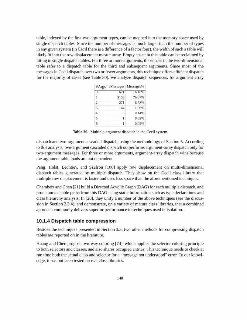
148

table, indexed by the first two argument types, can be mapped into the memory space used bysingle dispatch tables. Since the number of messages is much larger than the number of typesin any given system (in Cecil there is a difference of a factor four), the width of such a table willlikely fit into the row displacement master array. Empty space in this table can be reclaimed byfitting in single dispatch tables. For three or more arguments, the entries in the two-dimensionaltable refer to a dispatch table for the third and subsequent arguments. Since most of themessages in Cecil dispatch over two or fewer arguments, this technique offers efficient dispatchfor the majority of cases (see Table 30). we analyze dispatch sequences, for argument array

dispatch and two-argument cascaded dispatch, using the methodology of Section 5. Accordingto this analysis, two-argument cascaded dispatch outperforms argument-array dispatch only fortwo-argument messages. For three or more arguments, argument-array dispatch wins becausethe argument table loads are not dependent.

Pang, Holst, Leontiev, and Szafron [108] apply row displacement on multi-dimensionaldispatch tables generated by multiple dispatch. They show on the Cecil class library thatmultiple row displacement is faster and uses less space than the aforementioned techniques.

Chambers and Chen [21] build a Directed Acyclic Graph (DAG) for each multiple dispatch, andprune unreachable paths from this DAG using static information such as type declarations andclass hierarchy analysis. In [20], they unify a number of the above techniques (see the discus-sion in Section 2.3.4), and demonstrate, on a variety of mature class libraries, that a combinedapproach commonly delivers superior performance to techniques used in isolation.

10.1.4 Dispatch table compression

Besides the techniques presented in Section 3.3, two other methods for compressing dispatchtables are reported on in the literature.

Huang and Chen propose two-way coloring [74], which applies the selector coloring principleto both selectors and classes, and also shares occupied entries. This technique needs to check atrun time both the actual class and selector for a “message not understood” error. To our knowl-edge, it has not been tested on real class libraries.

#Args #Messages Messages%

0 671 16.16%

1 3159 76.07%

2 271 6.53%

3 44 1.06%

4 6 0.14%

5 1 0.02%

6 1 0.02%

Table 30. Multiple-argument dispatch in the Cecil system

149

Thorup presents sparse arrays [122], used to implement Objective-C, which find a methodthrough two indirections. The storage of empty entries is reduced by dividing a dispatch tableinto chunks of constant size, and not storing those that are completely empty. No fill rates orother comparable data is reported, so we can not compare the memory requirements with ourtechnique. However, the dispatch speed of sparse arrays is lower because of the double memoryindirection.

Compression of sparse tables is an old problem. Dencker et. al., in [34], list a number of tech-niques for the compression of parser tables, which contain large numbers of default entries. Forthis application, accessing a table entry is time critical, changing the table is not. Therefore therequirements are identical to those of dispatch tables. However, of the techniques presented,only row displacement and selector coloring perform retrieval in constant time. The other tech-niques, like run length encoding, require search within the compressed table.

We used a genetic algorithm to find near-optimal column and row numbers for arbitrary sparsetables [41]. This experiment showed that better encodings exist than the heuristics employed inclass-based row displacement [40]. However, the time required to find these encodings wasprohibitive in the context of dispatch table compression (several hours on a Cray Y-MP).

150

10.2 Hardware techniques

10.2.1 Indirect branch prediction

Lee and Smith [89] describe several forms of BTBs. Jacobson et al. [77] study efficient ways toimplement path-based history schemes and observe that BTB hit rates increase substantiallywhen using a global path history. Their Correlated Task Target Buffer (CTTB), unconstrainedand fully associative, reached misprediction rates of 18% and 15% forgcc andxlisp with pathlength 7; our study found misprediction rates of 12% and 1.5% forp=7. The different results canbe explained by several factors: different benchmark version (SPEC92 vs. SPEC95), inputs, andradically different architectures (e.g., the multiscalar processor’s history information will likelyomit some branches in the immediate past). Finally, Jacobson et al. include conditionalbranches in the path histories, which is probably responsible for the difference inxlisp .

Chang et al. [25] explore a limited range of two-level predictors for indirect branches and simu-late the resulting speedups of selected SPECint95 programs for a superscalar processor. Themisprediction rate of a BTB-2bc is reduced by half to 30.9% forgcc with a Pattern HistoryTagless Target Cache with configuration gshare(9). This predictor XORs a global 9-bit historyof taken/non taken bits from conditional branches with the branch address, and uses the resultas a key into a globally shared, tagless 512-entry history table. In the present study, a compa-rable non-hybrid predictor (p=3, tagless 512-entry) reaches a misprediction ratio of 31.5% forgcc, the best non-hybrid predictor (p=2, four-way associative 512-entry) has 28.1% mispredic-tion rate, and the best dual-path hybrid predictor (p1=3, p2=1, four-way associative 512-entry)reaches 26.4%. These comparisons should be regarded with caution, since the two experimentsdiffered in architectures (HPS vs. SPARC), compilers, and benchmark inputs.

Emer and Gloy [54] describe several single-level indirect branch predictors based on combina-tions of the values of PC, SP, register number, and target address, and evaluate their perfor-mance on a subset of the SPECint95 programs. For these programs, the best predictor shownachieved a misprediction ratio of 30%, although the authors allude to a better predictor thatachieves 15%.

Calder and Grunwald proposed the two-bit counter update rule for BTB target addresses [14]and showed that it improved the prediction rate of a suite of C++ programs.

Stark, Evers and Patt [118], determine the best path length for each branch in the program byprofiling, and communicate this path length to the hardware through the ISA. This is a refine-ment of branch classification, with 32 branch classes, each corresponding to a particular pathlength. For a tagless table of 128 entries, a misprediction rate of 27.7% is achieved for gcc. Thistechnique represents the most fine-grained profile-based classification of indirect branches weknow of.

Kalamatianos and Kaeli [81] apply PPM prediction (see Section 10.2.2.2) to indirect branches,demonstrating excellent accuracy. The PPM predictor shortens a history pattern bit by bit, and

151

looks it up in successively smaller stages. Each stage is half the size of its predecessor. The bitscorrespond to branch targets, so this scheme tests ever shorter path lengths. This resembles theprediction rule of a cascaded predictor. Cascaded prediction differs from PPM predictionbecause a cascaded predictor employs pattern filtering and uses a separate history buffer foreach stage.The number of stages is also independent from pattern length, and each stage can useany table size. Although Kalamatianos and Kaeli’s study [81] demonstrates slightly betterprediction performance on some of the benchmarks measured here, at least part of the improve-ment is due to dynamic classification of indirect branches into two classes: a class that corre-lates best with a history buffer which stores both conditional and indirect branch targets, andone that correlates best with only indirect branch targets. In this study we use a purely indirectbranch target trace.

10.2.2 Prediction architectures

This study builds on previous work in conditional branch prediction. Many alternative imple-mentations were conceived by adapting existing conditional branch prediction architectures toindirect branches. The literature on conditional branch prediction is extensive. We refer to Uhtet al. [123] for a recent general overview, and limit the discussion to work which is closelyrelated to this study.

10.2.2.1 Basic prediction

Yeh and Patt first proposed two-level branch prediction [134] and presented a thorough classi-fication [135] of two-level predictors, which influenced the work discussed in Section 8.2.

Nair [105] introduced path-based branch correlation for conditional branches and showed thata path-based predictor with two-bit partial addresses attained prediction rates similar to apattern-based predictor with taken/not taken bits (for similar hardware budgets).

Talcott’s disseration work [120] influenced much of this study, and the Powersim simulatorwhich he used to do cycle-level simulation was adapted to the SPARC architecture and used inthe experiments of Section 6.

Juan, Sanjeevan and Navarro [80] extend the two-level predictor with a table that measuresprediction accuracy and adapts the path length of a two-level predictor dynamically in order toimprove prediction accuracy over individual programs in a benchmark suite. Although thisproposal is an improvement over a statically chosen path length, it still seems too coarse-grained for optimal performance. Hybrid predictors, as discussed in Section 9, allow individualbranches or even history patterns, rather than individual programs, to settle on a path lengthwhich best predicts the branch.

152

10.2.2.2 Hybrid prediction

McFarling first proposed to combine basic predictors into a hybrid predictor [98]. SeeSection 9.1.2 for a detailed discussion. Chang, Hao and Patt’s study [24] and Evers, Chang andPatt’s [56] present more recent results of hybrid conditional branch prediction.

Chang, Hao and Patt [23] first proposed branch classification for conditional branches. Condi-tional branches are divided in six classes, corresponding to the frequency with which a branchis taken in a profiling run, with boundary values 5%, 10%, 50%, 90%, 95% and 100%. Theauthors present a GAs predictor with multiple branch history length and shared history table,which is similar to the classifying shared-table hybrid predictor used in this study. A dynami-cally classifying predictor uses a fully associative branch address cache (BAC), consisting of 2-bit saturating counters that indicate the component predictors which best predicts a givenbranch. Since we use a simple predictor both to predict indirect branches and to classify themas “hard-to-predict”, a BAC is unnecessary in a dynamically classifying cascaded predictor. Bycombining profile-guided classification for mostly monomorphic branches with dynamic clas-sification for mixed-direction branches (between 10% and 90% taken), prediction accuracy of96.4% is achieved for conditional branches of the SPECint92 benchmarks suite.

Stark, Evers and Patt [118] determine a path length per branch by profiling each branch in aseparate profiling run. Their technique is an instance of profile based classification which ismuch more fine-grained than the classifications used in Section 9.2 (see Section 10.2.1 for moredetail).

Cheng, Coffey and Mudge [28] propose Partial Prefix Matching (PPM) prediction, based on acompression technique, for conditional branch prediction. They show that a PPM predictorperforms better than a two-level predictor for a similar hardware budget. Since a PPM predictorpredicts for the longest pattern for which a prediction is available (choosing progressivelyshorter path lengths until a prediction is found), a cascaded predictor mimics this behavior.However, PPM prediction has a predetermined table size for all its components (exponentiallydecreasing in size), reserves a component for each history bit length, and does not employfiltering (similar to the ideal staged predictor discussed in Section 9.4.3.2).

Federovsky, Feder and Weis [57] also adapt a compression technique, Context Tree Weighting(CWT), to conditional branch prediction. They demonstrate that the technique delivers excel-lent prediction accuracy under the assumption of unconstrained hardware resources. They donot assess prediction performance under limited hardware budgets.

Eden and Mudge [52] proposed the YAGS architecture for conditional branch prediction. AYAGS predictor uses two kinds of predictor tables. A direct-mapped table (the choice table)stores the dominant direction of a branch using a 2-bit counter. Two tagged tables (directiontables) store a prediction for a pattern that represents history as taken/non taken bits. One ofthese is used for branches that are mostly taken, the other for branches that mostly not taken.Prediction in a direction table takes precedence over the prediction in the choice table, and

153

patterns enter a direction table only if the choice table mispredicts. This scheme resembles a 2-stage cascaded predictor with a direct-mapped BTB as first stage. The main difference is thatthe second stage of a YAGS predictor consists of two separate tables. However, the authorsagreed that this is not a requirement. A YAGS predictor shows better prediction accuracy thanother conditional branch predictor schemes. We believe this is evidence that cascaded predic-tion is also likely to perform well on conditional branches.

Table update filtering, as used in a cascaded predictor, has a precursor in conditional branchprediction: Chang, Evers and Patt [22] study a conditional branch predictor which uses a BTBto filter out easily predicted branches. Their predictor inhibits the history table update if theBTB’s confidence counter is at maximum (e.g., “strongly taken”). See Section 9.4.1.1 for amore detailed discussion and comparison with the filtering rule of cascaded predicition.

154

155

11 Future work and open problems“Speed is exchangeable for almost anything. Anycomputer can emulate any other at some speed”,

Burton J. Smith [115]

“Sometimes it is good that some things are impos-sible. I am happy there are many things thatnobody can do to me.”

Leonid Levin [115]

Much work remains to be done in every field we explored in the course of this study. The designspace of software techniques is by no means exhausted. Both hardware and compiler techniquescontinue to evolve at a rapid pace, making continuous evaluation of dispatch cost necessary.The population of programs that run on the majority of processors also changes, as differenttrends emerge in the market place. Adaptivity, both in software and hardware, and across thesoftware/hardware interface, seems to provide a general solution to many efficiency problems,but it has barely been explored. Finally, the hardware techniques explored for indirect branchprediction may have a wider application domains.

11.1 Software techniques

11.1.1 Inline caching with fast subtype tests

It is entirely feasible to replace the equality test in the inline cache method prefix (seeSection 3.2.2) with a subtype test. Recent advances in fast subtype testing, explored by Krall,Vitek and Horspool [85], suggest that such a test can be implemented in only a few assemblyinstructions. The advantage of subtype testing is that the current receiver class does not need tobe identical to the last observed class, but can be a descendant of a common super class,provided that the implementation is not overridden along the way. The inline cache may thusachieve a higher hit rate. An disadvantage of such a scheme is the requirement that the subtyperelationship can be trusted. Whenever the class hierarchy changes, inline caches must bechecked for correctness. A standard inline cache is more responsive, since a changed class canbe assigned a new identity, so that old cache information results in a miss and causes an update.

11.1.2 Global caching with history

A global cache (see Section 3.2.1) is like a BTB: for every class/selector combination, exactlyone target is stored. If the key into the cache were augmented with a history of previous targets,much higher hitrates may be achieved (a global cache is less accurate than an inline cache).Since global caches are easy to implement, they are the preferred form of optimization in manymid-level systems. With little extra effort, a costly dispatch table search may be avoided moreoften.

156

11.2 The software-hardware interface

11.2.1 Measuring cycle cost of more software techniques on superscalarprocessors

We only measured virtual function table dispatch on a range of superscalar processor designs.To evaluate other table-based techniques, in particular row-displacement dispatch, and variousforms of inline caching, these techniques should be implemented in full in the context of a realprogramming environment. Hybrid techniques, that use inline caching but resort to a more effi-cient table-based technique in the miss case, can reduce dispatch cost further on processors thatlack indirect branch prediction. The SUIF project [84], for instance, is an appropriate researchvehicle for this work.

11.2.2 Benchmarking Java

With the growing popularity of Java, processors are likely to see more code generated by a Javacompiler. Java programs are different from C++ programs. Although the all-virtual versions ofC++ programs in Section 6 capture part of the behavior of their Java counterparts by forcing theJava default (non-final) on member function declarations, it would be nevertheless expedient todirectly measure Java applets.

11.2.3 Influence of code-rewriting techniques on indirect branchpopulation

Since code-rewriting techniques are capable of removing monomorphic indirect branches fromthe executable, they can change the nature of the indirect branch stream that the micro-archi-tecture must predict. With statically predicted branches removed from the indirect branchstream, capacity misses will likely diminish, while the remaining indirect branches will be, onaverage, harder to predict accurately. Hölzle [71], shows that inlining, by removing near-mono-morphic calls, increased the dynamic average number of targets (arity) of the remaining calls bymore than a factor two. This may take some load off the first stage of a cascaded predictor, sincefewer easily predicted branches reach the hardware, resulting in overall reduction of dispatchcost.

Some code-rewriting techniques are capable or over-optimization. For instance, a recentlyproposed technique for Java dispatch, by Zendra, Colnet and Collin [136], replaces all polymor-phic calls by a tree of nested conditional branches. Whether this is a win depends on whether theprocessor’s indirect or conditional branch prediction architecture is best suited to capture theregularity of target patterns of the branch. It may well be the case that this kind of optimizationreduces performance, as in the case where an inline cache uses an inferior form of prediction,assuming that the hardware does not predict indirect branches at all.

157

11.2.4 Feedback from predictor hardware to code-rewriting techniques

Type-feedback, in combination with dynamic recompilation of a program’s “hot spot’s” hasproven a very effective tool for program optimization in a dynamic environment [71]. Twostatistics are gathered by the run-time system: the types that occur as receivers of a particularmessage call site and the frequency of invocation of each particular message implementation.The latter tells the dynamic (JIT) compilation system which methods are executed frequentlyenough so that it is worth paying a run-time recompilation cost. The former tells the optimizerwhich polymorphic calls are, at least temporarily, dominated by one or only a few targets, sothat these can be inlined, enabling classic compiler optimizations and further reducing type testswithin the inlined code. The overhead, compared to an off-line profiling optimizer (assumingthe program’s behavior is relatively constant) consists of the actual compilation cost, occurringat run time, and the cost of updating type feedback information and invocation counters. Typefeedback can be supported by hardware.

Branch prediction hardware, by its very nature, stores statistical information about branchtargets in its history table. Suppose we collect, from the history table, all targets that occur fora particular call site (an indirect branch address1). This gives us, in the case of a BTB, the targetthat occurred most recently2 for recently executed call sites. If the BTB is sampled regularly,frequency information can be obtained from a) the presence of a target in the table, b) it’s place(assuming LRU replacement) in the associativity set to which it belongs. Branch predictionhardware can therefore not only speed up non-inlined dispatch sequences, it can also, at littleextra cost, suggest opportunities for inlining to a dynamic compiler. It can therefore free therun-time system from the burden of continually updating invocation counters and polymorphicinline caches (which speed up dispatch and provide type-feedback in SELF). We only need toaugment the architecture with an instruction to block-dump the BTB in memory. Periodicalbranchmaps can be processed by measuring the difference with the previous one. The size ofthis delta can signal state changes in the program, and the persistent entries can designateinlining opportunities to the dynamic compiler. This may prove a useful framework to adap-tively tune the recompilation strategy, for instance by increasing the sampling frequency formore reactive recompilation, or lowering it for settled systems, to reduce the run-time overheadof BTB sampling. The effectiveness of hardware-supported type-feedback, or target feedback,is still an open problem.

Merten et al. [99] propose a separate hardware device for detecting program hot spots. TheirBranch Behavior Buffer (BBB) closely resembles a BTB, but is augmented with counters todetect the frequency of branch execution. In future work, they envision to take advantage ofbinary reoptimization opportunities enabled by using the information in the BBB.

1 This has to be stored as a separate address, or, with only slight loss of prediction accuracy, instead of the tag in an associativetable. A tag comparison becomes a comparison with the branch address. In early experiments we disambiguated entries this way,and misprediction rates were fairly similar to that of tags checking for identity of a the key pattern (history pattern XOR address).2 With the adjustment that 2-bit counters filter out targets that occur in isolation.

158

11.3 Exploring different applications for hardware-basedprediction

The new prediction architectures in this study may well prove advantageous in other applicationdomains than indirect branch prediction, such as:

• Conditional branch prediction: the Pentium II conditional branch target predictor (512entries with for each a 4-bit local history), arguably the currently most popular predictor inpractice, is a two-level predictor. It seems likely that cascaded prediction with leakyfiltering will reduce cold-start and capacity misses as it does for indirect branches, sincemany conditional branches behave monomorphically. Chang, Evers and Patt [22]demonstrate the potential of table update filtering on conditional branches, using a differentfiltering rule (see the discussion in Section 9.4.1.1).

• Value prediction: this is currently an active field. Again, cascaded prediction may proveadvantageous, since the value equivalent of a monomorphic branch is a constant. Run timeconstants occur frequently enough to warrant special treatment, as indicated in Lipasti,Wilkerson, and Shen’s seminal paper [93]. They propose a constant verification unit thatstores highly predictable and constant values.

• Prefetching: if the history table is augmented to store multiple alternative targets, whichserve as hints to the prefetcher as to which code sequences are likely to be needed in theinstruction cache, the cache missrate could be reduced. Each target could keep a counter toindicate the likelihood of its occurrence.

• Predict-ahead: when the history table stores the address of the next indirect branch as wellas the target address, the predictor can run arbitrarily far ahead of execution. The averagelength of a precisely predicted sequence of targets equals the reciprocal of themisprediction rate. With an achievable prediction rate of 95%, an average of 20 branchescould therefore be predicted ahead of time. This can be useful in all the previous applicationdomains. The Rise mP6 processor [116] uses predict-ahead as part of its fetch unit: thetarget of theprevious branch (not theaddress of thecurrent branch) is used to look up thenext target prediction in a BTB. Up to four targets can be predicted ahead of time.

• Compression: the link between compression and prediction has been pointed out multipletimes in the literature (see Section 10.2.2.2). Compression of arbitrary traces can beaccomplished by storing a trace consisting of the runlength of precisely predicted valuesand the next mispredicted value, along with a predictor specification. Accurate run-aheadprediction architectures may thus enable the building of fast, economic compressionhardware.

159

11.4 Algorithms

The loss of prediction performance due to hardware constraints is an algorithmic issue. Thisstudy explores, for a limited application domain, the performance of indirect branch targetpredictors, hampered by limited resources and committed to simple prediction logic (so as toremain practical in hardware). These designs only scratch the surface of what is possible whenthe latency of the operation and the size of its memory resources is not as restricted as in hard-ware. In less constrained, less time-critical domains than branch prediction, much lowermisprediction rates could be achieved.

Since trace prediction has many applications, a rigorous study on the mechanics of limitedresource prediction may be both desirable and profitable. Prediction architectures similar tothose presented in branch prediction literature may have applications on all kinds of domainsthat deal with strings. We envision applications in compression, fast string matching (forexample in gene sequencing of DNA string representations), and user interface event anticipa-tion.

11.5 Misprediction rate as a program complexity metric

A program with easily predicted branches is a simple program.Go, the SPECINT benchmarkthat implements a strategy for playing Go, is notoriously hard to predict. Part of the reason isthat indirect branches occur very infrequently ingo (once every 50K instructions), so that theindirect branch trace captures only a small part of the overall execution path. 80% predictionaccuracy seems fairly good, considering this context. In contrast, we believe that the highmisprediction rate of for instancejhm (with less than 50 instructions between indirect calls, forthe best hybrid: 8%, the highest in the AVG-100 class), is due to the structural complexity of theJava class files it processes. If values, conditional branches and indirect branches are predicted,a program’s behavior can be quantified as X,Y, with X the misprediction rate for a particularpredictor configuration Y. This may be a practical way to quantify program executioncomplexity. Ideal predictors, which lack the noise of capacity, conflict and pattern interferencemisses, could be used to establish equivalence classes of complexity.

160

161

12 Conclusions“We didn’t know what we wanted and how to doit. It just sort of grew....it was a big problem andwhat we did looks astonishingly clumsy now”,John Backus on the invention of Fortran [115]

Though we don’t claim to have discovered something as fundamental to computer science as ahigh-level language compiler, we have struggled hard to optimize a high-level languageconstruct: polymorphic calls. We have gathered substantial evidence that software- and hard-ware-based support for polymorphic call resolution is useful, effective and affordable, and,according to current projections, will become more so in the next decade.

Polymorphic call optimization is useful because polymorphic calls are expensive. We measureda number of industry-size object-oriented programs and found that the most efficient andpopular call resolution technique costs up to 30% of execution time. Since these programs arewritten in C++, where polymorphic calls are not the default case, it is likely that the growingpopularity of fully polymorphic languages like Java will expose even more polymorphism tofuture processors. Near-future processors with high clock frequency need deep instruction pipe-lines, which are likely to increase the cost of a polymorphic call.

Polymorphic call resolution techniques are effective in reducing the run-time call cost. Westudied both software and hardware techniques:

• In the software domain, we have analyzed current dispatch techniques qualitatively andquantitatively. This study showed that inline cache strategies can outperform table-basedtechniques by predicting indirect branches in software, even though they show bad worst-case performance. However, if hardware-based prediction is present, table-based softwaretechniques win. We have increased the application domain of table-based call resolution byusing row displacement compression on dispatch tables. Dynamically typed and multipleinheritance languages can now also use fast table-based dispatch. Row displacementcompression is used in at least one industrial strength programming system, JOVE [133], aJava compiler designed to handle very large applications1.

• In the hardware domain, we have studied dedicated indirect branch predictionarchitectures. Simple prediction architectures, similar to software-based prediction, canreduce the frequency of mispredicted branches by a factor four (BTB, 256 entries, 25%misprediction). More sophisticated techniques, some of which have been first presented inthis work, can reduce misprediction frequency by a factor twenty (Cascaded, 3x2K entries,5% misprediction). Table-based call resolution thereby becomes nearly as efficient as aprocedural call, since only one out of twenty calls incurs a branch penalty.

1 Though statically typed, the use of interfaces in Java necessitates compression of interface dispatch tables. These incur memoryoverhead like multiple inheritance dispatch tables, since they allow the merging of dispatch tables from classes unrelated bysubclass (implementation) inheritance.

162

Polymorphic call support is affordable. Table-based dispatch techniques require affordable off-chip memory (4Mbytes for Self). The extra compilation time required to build the tables isnegligible compared to total compilation cost (2.5 seconds for Self on a 60 MHz Sparc-20).Hardware indirect branch prediction starts paying off at low on-chip transistor budgets (a 32entry BTB already predicts more than 70% of all indirect branches), and reaches 90% predict-ability for reasonable predictor table sizes (64+256 cascaded). In the next decade, uniprocessorsmay reach one billion transistors, with 48 million transistors dedicated to branch prediction[109]. Our study, and that of others [14][25][81] justifies that some of those transistors be spenton dedicated indirect branch prediction.

We believe that, using techniques as described in this dissertation, polymorphic call overheadcan become negligible in all but the most time-critical applications. This enlarges the applica-tion domain of object-oriented programming, allowing programmers to use polymorphism asthe default, instead of the exception. From our own experience in building software architec-tures, we consider this a Good Thing.

163

13 Glossary“‘Tis but thy name which is my enemy;Thou art thyself, though not a Montague.What’s a Montague? It is nor hand, nor foot,Nor arm, nor face, nor any other partBelonging to a man. O, be some other name!What’s in a name? That which we call a roseBy any other word would smell as sweet”,

Shakespeare [114]

Branch classification. A classifying hybrid predictor assigns to each branch a branch class.All branches that belong to a class use the same component predictor. Section 9.2

BTB. A table that stores the most recent target address of a branch instruction. Section 6.2.1

Cascaded predictor. A cascaded predictor classifies branches dynamically by observingtheir performance on a simple first-stage predictor. Only when this predictor fails to predict abranch correctly is a more powerful second-stage predictor permitted to store predictions fornewly encountered history patterns of that branch. If both stages have a target prediction, thelater stage takes precedence. Section 9.4

Dynamic caching. A message dispatch technique that caches the target of a message send atrun time. If the class of the receiver object is the different from that of the cached target, abackup message dispatch technique is invoked and the cache entry is replaced with the newtarget. Section 3.2

Dynamic typing. A typing regime which does not require that variables are annotated with atype at compile time. At run time, a variable can contain any object type. Section 2.3.1

Dual-path hybrid predictor . A hybrid predictor with two components of different pathlength. Section 9.3

Duomorphic branch. A branch that jumps to two targets during an entire program run.Section 9.2.2

Hybrid predictor . A branch predictor that combines two or more simpler predictors andchooses for each branch which component to trust. Section 9.1

Indirect branch . A branch instruction which transfers control to a target address stored in amachine register. Section 1.3

Indirect branch prediction . The process of predicting the target of an indirect branchinstruction, using only its address and possibly history information. Section 8

Inheritance. Incremental construction of classes (object types). A class is defined byextending an existing class, called its super class, by adding or redefining inherited functions.Section 1.2.1

Inline caching. A form of dynamic caching. Instead of storing a receiver class/messageselector pair with its resulting target method in a table, a direct call to the target replaces the callto the message dispatch routine. Section 3.2.2

164

Message dispatch. Polymorphic call resolution in object-oriented languages. The dispatchfunction takes as arguments the class of the current object (the receiver), and the name of thecalled message (selector), and maps this pair to the appropriate implementation (method).Section 2.3

Metaprediction. The mechanism used in a hybrid predictor to decide which componentprediction to trust (predict which prediction is best). Section 9.1.2

Monomorphic branch. A branch that jumps to only one target during an entire program run.Section 9.2.2

Multiple dispatch . A generalization of message dispatch. The run time target of a messagedepends on more than one argument, where single dispatch only takes the receiver’s type (firstargument) into account. Section 2.3.3

Multiple inheritance . An inheritance regime which allows a class to inherit from anynumber of super classes. Section 2.3.2

Polymorphic call. A polymorphic call looks like a procedural call, but where a proceduralcall has only one possible target subroutine, a polymorphic call can result in the execution ofone of several different subroutines. The choice is typically based on the type of the first argu-ment, and is made at run time. Section 1

Polymorphic call resolution. The action of mapping a polymorphic call to a single target atrun time. Section 1.2

Predicate dispatch. A generalization of multiple dispatch. The run time target of a messagedepends on a predicate expression, which can be an arbitrary side-effect free expression in theunderlying programming language. The most powerful form of polymorphism. Section 2.3.4

Single inheritance. An inheritance regime which requires that a class inherits from at mostone super class. Section 2.3.2

Staged predictor. A cascaded predictor without filtering. Section 9.4.3

Static caching. seeTable-based dispatch.

Static typing. A typing regime which requires that all variables in a program are annotatedwith a type at compile time. At run time, a variable can contain only objects of the declared typeand its subtypes. Section 2.3.1

Subclassing. Implementation by incremental modification of classes through inheritance. Aclass inherits all functions from its super class, but can override them (redefine their implemen-tation) and add new functions. Section 1.2.1.2

Subtyping. Incremental interface definition through inheritance. A subtype must implement atleast all functions of the type it is derived from. Section 1.2.1.1

Table-based dispatch. A message dispatch technique that precomputes all valid combina-tions of class/selector pairs at compile or link time. At run time, dispatch is accomplished bysimple table lookup, typically a small number of dependent array accesses. Section 3.3

Appendix A Basic prediction accuracy per benchmark

Table A-1 shows the misprediction rates (in %) per benchmark and averages for a fully associa-

tabl

esiz

e

btb

fulla

ssoc

tagl

ess

asso

c1

asso

c2

asso

c4

fulla

ssoc

hybr

id a

ssoc

4

btb

fulla

ssoc

tagl

ess

asso

c1

asso

c2

asso

c4

fulla

ssoc

hybr

id a

ssoc

4

AVG idl32 28.11 30.71 32.50 30.28 25.98 22.62 25.98 6.09 6.76 6.39 6.15 7.87 8.06 7.8764 26.83 24.26 26.30 23.60 19.77 18.53 19.77 2.99 5.20 6.38 5.55 5.33 5.02 5.33128 25.76 20.56 22.22 19.09 16.98 15.56 16.66 2.45 4.80 4.54 3.73 2.74 3.77 3.64256 25.13 16.99 18.06 15.15 13.73 12.47 13.29 2.41 3.40 3.13 3.69 2.67 1.23 2.10512 25.01 13.74 15.92 12.59 11.35 10.40 10.90 2.40 2.05 3.26 2.18 1.49 1.05 1.171024 24.93 11.74 13.53 10.74 9.82 8.48 8.98 2.40 1.43 2.38 1.33 0.85 0.64 0.762048 24.92 10.27 11.48 9.49 8.52 7.76 7.82 2.40 1.13 1.80 0.82 0.69 0.62 0.464096 24.92 9.12 10.43 8.54 7.77 7.17 6.72 2.40 0.95 1.60 0.71 0.63 0.62 0.388192 24.92 8.45 9.68 8.02 7.27 6.57 5.95 2.40 0.69 1.01 0.67 0.63 0.44 0.3716384 24.92 7.77 8.97 7.47 6.81 6.14 5.53 2.40 0.69 0.85 0.65 0.45 0.42 0.3632768 24.92 7.09 8.46 7.07 6.57 6.02 5.21 2.40 0.55 0.81 0.50 0.45 0.42 0.35

100-AVG ijpeg32 14.97 18.92 18.07 16.82 16.81 15.86 16.81 1.26 26.62 1.52 1.64 0.82 0.32 0.8264 13.31 15.73 16.96 14.68 14.29 13.76 14.29 1.26 26.63 51.15 0.31 0.31 0.31 0.31128 11.72 15.01 13.98 12.33 11.77 13.63 12.35 1.26 0.92 0.56 0.31 0.31 0.39 0.29256 10.57 12.49 12.01 12.11 11.20 9.85 10.08 1.26 0.69 0.56 0.65 0.39 0.39 0.29512 10.32 9.84 12.27 9.84 9.09 8.20 8.22 1.26 0.44 0.39 0.39 0.39 0.39 0.371024 10.14 8.42 10.77 8.48 7.15 6.37 6.66 1.26 0.45 0.39 0.39 0.46 0.46 0.372048 10.11 7.41 9.21 6.97 6.37 6.12 5.96 1.26 0.45 0.39 0.46 0.46 0.51 0.384096 10.11 6.69 8.54 6.29 5.77 5.62 5.47 1.26 0.44 0.39 0.46 0.46 0.51 0.478192 10.11 6.21 6.91 5.92 5.62 5.26 4.83 1.26 0.50 0.46 0.46 0.51 0.56 0.4716384 10.11 5.95 6.43 5.69 5.42 4.93 4.54 1.26 0.56 0.46 0.51 0.56 0.62 0.4732768 10.11 5.56 6.10 5.68 5.26 4.86 4.42 1.26 0.56 0.46 0.56 0.56 0.62 0.48

200-AVG ixx32 39.38 40.82 44.86 41.81 33.84 28.40 33.84 46.58 33.15 56.21 51.11 30.07 24.30 30.0764 38.42 31.58 34.30 31.24 24.48 22.61 24.48 45.75 24.47 32.91 24.86 18.10 15.94 18.10128 37.79 25.32 29.28 24.89 21.44 17.22 20.36 45.70 24.60 27.55 17.93 15.37 12.10 19.02256 37.61 20.84 23.24 17.77 15.91 14.72 16.04 45.70 18.74 20.58 15.47 12.57 10.34 13.32512 37.61 17.08 19.05 14.94 13.29 12.28 13.20 45.70 13.88 21.38 13.48 10.63 10.25 9.481024 37.61 14.58 15.90 12.67 12.10 10.28 10.98 45.70 12.37 15.32 11.57 9.03 8.21 8.562048 37.61 12.73 13.43 11.65 10.36 9.16 9.42 45.70 10.90 12.51 9.82 8.47 6.94 6.064096 37.61 11.21 12.05 10.46 9.47 8.51 7.80 45.70 9.34 12.11 9.29 8.29 6.94 5.068192 37.61 10.37 12.06 9.82 8.69 7.69 6.91 45.70 8.86 11.28 8.94 7.11 5.86 4.9116384 37.61 9.32 11.15 9.00 8.00 7.18 6.38 45.70 7.66 10.55 8.04 5.98 5.58 4.7032768 37.61 8.39 10.48 8.26 7.68 7.01 5.88 45.70 6.79 10.14 6.70 5.94 5.58 4.15

INFREQ-AVG lcom32 31.78 31.68 32.32 31.88 20.85 17.95 20.85 5.18 12.99 5.80 5.24 4.81 4.45 4.8164 31.78 27.61 34.80 18.16 17.74 17.54 17.74 4.71 4.67 4.78 4.03 3.84 3.62 3.84128 31.78 23.16 20.75 17.96 17.54 15.66 21.46 4.46 4.75 3.90 3.61 3.47 3.49 3.72256 31.78 19.92 18.07 17.52 15.58 14.98 17.03 4.25 3.93 3.43 3.37 3.25 3.27 2.96512 31.78 15.26 20.34 16.44 15.18 14.97 11.31 4.25 3.25 3.26 2.80 2.60 2.53 2.561024 31.78 14.27 19.40 16.09 10.89 10.40 10.43 4.25 2.68 2.77 2.33 2.20 1.88 1.952048 31.78 13.54 18.06 12.86 10.67 10.16 10.09 4.25 2.17 2.43 1.85 1.68 1.65 1.694096 31.78 12.04 16.48 11.87 10.44 10.06 8.31 4.25 1.83 2.12 1.56 1.42 1.34 1.318192 31.78 12.12 14.41 11.76 10.50 10.81 7.84 4.25 1.62 1.71 1.44 1.36 1.34 1.1116384 31.78 12.66 14.17 11.67 11.22 9.17 8.60 4.25 1.55 1.58 1.37 1.37 1.39 1.0432768 31.78 11.14 13.98 11.89 11.07 9.10 8.90 4.25 1.43 1.49 1.39 1.35 1.39 1.02

OO-AVG m88ksim

Table A-1. Misprediction rates (per benchmark and averages) for basic predictors.

166

32 23.70 25.80 28.17 25.96 22.64 20.02 22.64 76.41 56.87 78.29 76.41 45.33 35.99 45.3364 22.18 20.43 22.55 18.96 17.18 16.04 17.18 76.41 46.52 49.25 35.99 35.99 35.99 35.99128 20.87 20.75 18.40 15.33 14.13 15.43 15.47 76.41 43.78 46.40 35.99 35.99 26.55 46.11256 19.97 17.00 15.48 14.79 13.29 11.95 12.16 76.41 36.17 35.99 29.46 26.55 26.55 32.27512 19.81 13.37 15.30 11.95 10.61 9.50 10.50 76.41 22.07 32.29 27.54 26.55 26.55 15.381024 19.69 11.29 12.63 9.91 9.47 7.93 8.49 76.41 20.16 30.44 27.54 14.40 14.40 13.562048 19.67 9.81 10.51 9.14 8.09 7.21 7.50 76.41 19.31 30.43 17.48 14.40 13.40 8.724096 19.67 8.67 9.68 8.21 7.38 6.70 6.48 76.41 15.41 30.43 14.58 14.40 13.40 2.178192 19.67 8.03 9.32 7.75 6.90 6.31 5.76 76.41 14.39 16.40 14.40 13.40 10.58 2.1716384 19.67 7.43 8.57 7.21 6.49 5.91 5.35 76.41 14.43 16.40 13.40 10.58 3.07 4.0032768 19.67 6.82 8.00 6.76 6.33 5.87 5.06 76.41 9.64 16.40 10.58 10.58 3.07 4.00

C-AVG perl32 34.91 36.72 37.28 35.94 27.18 23.20 27.18 31.80 60.62 31.81 31.80 36.31 22.80 36.3164 34.54 30.25 34.76 26.10 21.67 20.83 21.67 31.80 45.24 45.27 49.74 22.76 22.75 22.76128 34.27 21.65 25.78 22.75 20.46 15.76 20.41 31.80 0.37 40.74 36.21 22.72 0.34 0.29256 34.25 18.43 20.96 16.75 15.16 14.31 16.43 31.80 0.35 22.73 0.33 0.32 0.29 0.26512 34.25 14.90 18.84 15.23 14.10 13.69 11.56 31.80 0.31 0.33 0.32 0.29 0.28 0.271024 34.25 13.50 17.48 14.34 10.75 10.05 10.26 31.80 0.31 0.32 0.30 0.34 0.32 0.262048 34.25 12.43 15.87 11.56 10.08 9.57 9.31 31.80 0.30 0.31 0.34 0.33 0.37 0.274096 34.25 11.09 14.31 10.58 9.54 9.15 7.79 31.80 0.30 0.30 0.33 0.32 0.37 0.338192 34.25 10.75 12.45 10.19 9.31 8.98 7.12 31.80 0.34 0.35 0.33 0.37 0.40 0.3216384 34.25 10.60 12.02 9.87 9.38 7.91 7.26 31.80 0.38 0.34 0.37 0.40 0.45 0.3332768 34.25 9.42 11.73 9.82 9.08 7.72 7.22 31.80 0.38 0.33 0.41 0.40 0.45 0.34

SPEC-AVG porky32 34.05 35.89 34.75 34.29 25.64 21.58 25.64 21.70 28.88 26.38 23.76 22.52 19.41 22.5264 34.04 30.36 34.64 25.27 20.80 20.39 20.80 21.21 19.74 21.75 17.41 15.30 13.97 15.30128 34.02 20.11 25.21 22.61 20.19 14.91 19.45 21.08 19.24 17.53 13.97 13.15 9.68 16.11256 34.02 17.20 20.64 15.99 14.49 13.68 15.82 20.80 14.94 15.96 12.43 10.22 9.12 11.04512 34.02 13.72 18.12 14.80 13.78 13.48 10.70 20.80 12.28 12.53 10.16 9.01 8.90 9.281024 34.02 12.63 16.96 14.22 9.95 9.43 9.67 20.80 10.37 10.03 8.56 7.89 6.97 7.592048 34.02 11.72 15.46 11.00 9.49 9.02 8.99 20.80 9.30 8.96 7.78 6.88 5.13 6.994096 34.02 10.39 14.23 10.05 9.01 8.64 7.44 20.80 8.39 8.43 7.24 6.26 4.85 5.418192 34.02 10.12 11.76 9.71 8.67 8.56 6.76 20.80 7.22 9.13 6.98 5.30 5.05 5.0516384 34.02 10.22 11.39 9.26 8.79 7.35 7.01 20.80 6.07 7.68 5.64 5.22 4.61 4.7732768 34.02 8.95 11.13 9.32 8.51 7.13 7.05 20.80 5.37 6.53 5.19 4.99 4.61 4.29

beta self32 31.85 27.98 36.63 33.76 25.20 16.89 25.20 36.08 49.54 48.36 46.15 45.21 40.81 45.2164 30.48 21.88 23.13 19.59 14.73 12.22 14.73 32.34 44.08 46.73 39.69 38.86 36.39 38.86128 29.44 18.65 16.62 14.66 10.77 13.06 13.03 25.07 39.80 39.03 32.54 31.61 36.84 34.00256 28.57 13.88 12.88 13.04 10.99 10.44 10.17 18.41 33.05 32.08 31.53 29.44 26.91 26.15512 28.57 10.20 13.75 9.38 7.46 5.51 8.36 16.94 26.80 29.39 23.94 22.18 19.70 23.261024 28.57 7.84 10.64 6.04 5.61 3.19 4.92 15.88 22.37 24.27 19.48 18.61 16.62 17.112048 28.57 6.29 6.19 5.13 3.77 2.66 3.23 15.68 18.33 19.69 16.81 15.40 16.01 14.644096 28.57 4.42 4.78 4.12 3.28 2.63 2.20 15.68 15.49 16.84 14.03 12.90 13.44 13.388192 28.57 3.77 4.91 3.62 2.73 2.46 1.99 15.68 14.00 15.43 12.27 11.91 11.54 10.8316384 28.57 3.49 4.46 2.81 2.51 2.28 1.88 15.68 13.51 13.73 11.55 11.43 10.50 9.2532768 28.57 2.91 4.18 2.79 2.49 2.28 1.68 15.68 11.87 12.63 11.51 10.72 10.10 8.61

edg jhm32 40.88 42.59 54.99 47.48 37.97 34.57 37.97 11.45 14.05 12.24 11.81 14.40 14.03 14.4064 37.97 29.48 35.61 31.89 27.78 23.89 27.78 11.16 12.92 15.14 13.03 12.88 12.49 12.88128 35.99 32.48 29.80 23.77 22.36 21.72 27.08 11.13 15.12 12.22 11.96 11.76 13.36 11.81256 35.91 27.09 23.22 22.07 19.86 18.73 20.72 11.13 13.81 11.80 12.98 12.40 11.31 11.35512 35.91 23.17 23.84 18.18 16.36 15.18 17.57 11.13 12.75 14.64 12.18 11.27 10.59 11.001024 35.91 19.63 21.13 15.16 16.34 14.40 14.46 11.13 11.93 13.57 11.18 11.33 9.67 10.352048 35.91 17.40 18.73 15.53 14.19 13.46 11.59 11.13 11.59 13.03 12.10 10.92 9.41 9.85

tabl

esiz

e

btb

fulla

ssoc

tagl

ess

asso

c1

asso

c2

asso

c4

fulla

ssoc

hybr

id a

ssoc

4

btb

fulla

ssoc

tagl

ess

asso

c1

asso

c2

asso

c4

fulla

ssoc

hybr

id a

ssoc

4

Table A-1. Misprediction rates (per benchmark and averages) for basic predictors.

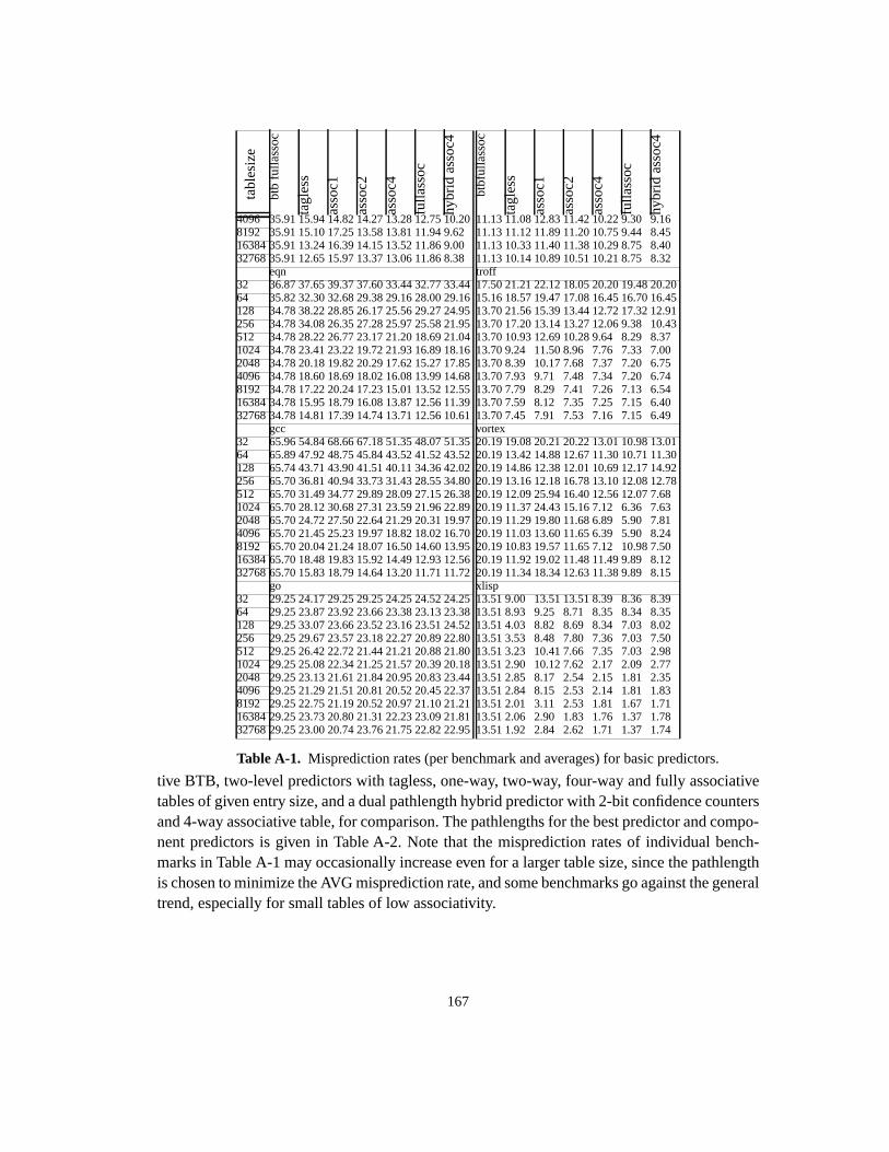
167

tive BTB, two-level predictors with tagless, one-way, two-way, four-way and fully associativetables of given entry size, and a dual pathlength hybrid predictor with 2-bit confidence countersand 4-way associative table, for comparison. The pathlengths for the best predictor and compo-nent predictors is given in Table A-2. Note that the misprediction rates of individual bench-marks in Table A-1 may occasionally increase even for a larger table size, since the pathlengthis chosen to minimize the AVG misprediction rate, and some benchmarks go against the generaltrend, especially for small tables of low associativity.

4096 35.91 15.94 14.82 14.27 13.28 12.75 10.20 11.13 11.08 12.83 11.42 10.22 9.30 9.168192 35.91 15.10 17.25 13.58 13.81 11.94 9.62 11.13 11.12 11.89 11.20 10.75 9.44 8.4516384 35.91 13.24 16.39 14.15 13.52 11.86 9.00 11.13 10.33 11.40 11.38 10.29 8.75 8.4032768 35.91 12.65 15.97 13.37 13.06 11.86 8.38 11.13 10.14 10.89 10.51 10.21 8.75 8.32

eqn troff32 36.87 37.65 39.37 37.60 33.44 32.77 33.44 17.50 21.21 22.12 18.05 20.20 19.48 20.2064 35.82 32.30 32.68 29.38 29.16 28.00 29.16 15.16 18.57 19.47 17.08 16.45 16.70 16.45128 34.78 38.22 28.85 26.17 25.56 29.27 24.95 13.70 21.56 15.39 13.44 12.72 17.32 12.91256 34.78 34.08 26.35 27.28 25.97 25.58 21.95 13.70 17.20 13.14 13.27 12.06 9.38 10.43512 34.78 28.22 26.77 23.17 21.20 18.69 21.04 13.70 10.93 12.69 10.28 9.64 8.29 8.371024 34.78 23.41 23.22 19.72 21.93 16.89 18.16 13.70 9.24 11.50 8.96 7.76 7.33 7.002048 34.78 20.18 19.82 20.29 17.62 15.27 17.85 13.70 8.39 10.17 7.68 7.37 7.20 6.754096 34.78 18.60 18.69 18.02 16.08 13.99 14.68 13.70 7.93 9.71 7.48 7.34 7.20 6.748192 34.78 17.22 20.24 17.23 15.01 13.52 12.55 13.70 7.79 8.29 7.41 7.26 7.13 6.5416384 34.78 15.95 18.79 16.08 13.87 12.56 11.39 13.70 7.59 8.12 7.35 7.25 7.15 6.4032768 34.78 14.81 17.39 14.74 13.71 12.56 10.61 13.70 7.45 7.91 7.53 7.16 7.15 6.49

gcc vortex32 65.96 54.84 68.66 67.18 51.35 48.07 51.35 20.19 19.08 20.21 20.22 13.01 10.98 13.0164 65.89 47.92 48.75 45.84 43.52 41.52 43.52 20.19 13.42 14.88 12.67 11.30 10.71 11.30128 65.74 43.71 43.90 41.51 40.11 34.36 42.02 20.19 14.86 12.38 12.01 10.69 12.17 14.92256 65.70 36.81 40.94 33.73 31.43 28.55 34.80 20.19 13.16 12.18 16.78 13.10 12.08 12.78512 65.70 31.49 34.77 29.89 28.09 27.15 26.38 20.19 12.09 25.94 16.40 12.56 12.07 7.681024 65.70 28.12 30.68 27.31 23.59 21.96 22.89 20.19 11.37 24.43 15.16 7.12 6.36 7.632048 65.70 24.72 27.50 22.64 21.29 20.31 19.97 20.19 11.29 19.80 11.68 6.89 5.90 7.814096 65.70 21.45 25.23 19.97 18.82 18.02 16.70 20.19 11.03 13.60 11.65 6.39 5.90 8.248192 65.70 20.04 21.24 18.07 16.50 14.60 13.95 20.19 10.83 19.57 11.65 7.12 10.98 7.5016384 65.70 18.48 19.83 15.92 14.49 12.93 12.56 20.19 11.92 19.02 11.48 11.49 9.89 8.1232768 65.70 15.83 18.79 14.64 13.20 11.71 11.72 20.19 11.34 18.34 12.63 11.38 9.89 8.15

go xlisp32 29.25 24.17 29.25 29.25 24.25 24.52 24.25 13.51 9.00 13.51 13.51 8.39 8.36 8.3964 29.25 23.87 23.92 23.66 23.38 23.13 23.38 13.51 8.93 9.25 8.71 8.35 8.34 8.35128 29.25 33.07 23.66 23.52 23.16 23.51 24.52 13.51 4.03 8.82 8.69 8.34 7.03 8.02256 29.25 29.67 23.57 23.18 22.27 20.89 22.80 13.51 3.53 8.48 7.80 7.36 7.03 7.50512 29.25 26.42 22.72 21.44 21.21 20.88 21.80 13.51 3.23 10.41 7.66 7.35 7.03 2.981024 29.25 25.08 22.34 21.25 21.57 20.39 20.18 13.51 2.90 10.12 7.62 2.17 2.09 2.772048 29.25 23.13 21.61 21.84 20.95 20.83 23.44 13.51 2.85 8.17 2.54 2.15 1.81 2.354096 29.25 21.29 21.51 20.81 20.52 20.45 22.37 13.51 2.84 8.15 2.53 2.14 1.81 1.838192 29.25 22.75 21.19 20.52 20.97 21.10 21.21 13.51 2.01 3.11 2.53 1.81 1.67 1.7116384 29.25 23.73 20.80 21.31 22.23 23.09 21.81 13.51 2.06 2.90 1.83 1.76 1.37 1.7832768 29.25 23.00 20.74 23.76 21.75 22.82 22.95 13.51 1.92 2.84 2.62 1.71 1.37 1.74

tabl

esiz

e

btb

fulla

ssoc

tagl

ess

asso

c1

asso

c2

asso

c4

fulla

ssoc

hybr

id a

ssoc

4

btb

fulla

ssoc

tagl

ess

asso

c1

asso

c2

asso

c4

fulla

ssoc

hybr

id a

ssoc

4

Table A-1. Misprediction rates (per benchmark and averages) for basic predictors.

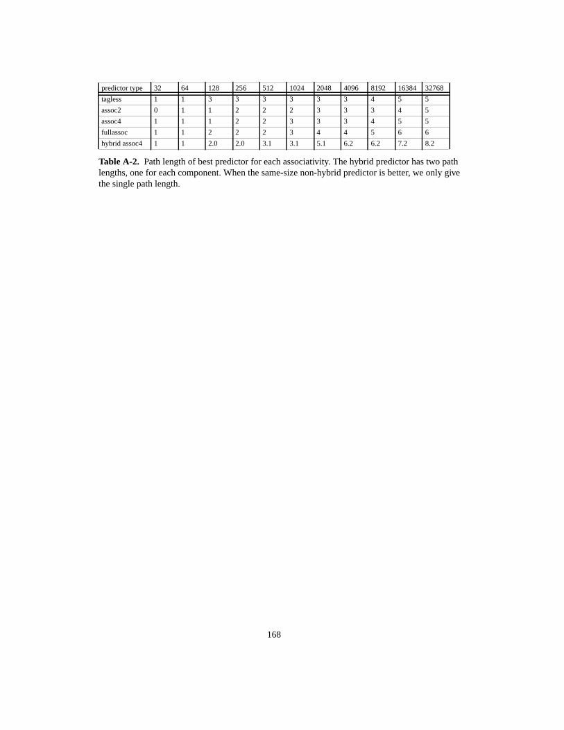
168

predictor type 32 64 128 256 512 1024 2048 4096 8192 16384 32768

tagless 1 1 3 3 3 3 3 3 4 5 5

assoc2 0 1 1 2 2 2 3 3 3 4 5

assoc4 1 1 1 2 2 3 3 3 4 5 5

fullassoc 1 1 2 2 2 3 4 4 5 6 6

hybrid assoc4 1 1 2.0 2.0 3.1 3.1 5.1 6.2 6.2 7.2 8.2

Table A-2. Path length of best predictor for each associativity. The hybrid predictor has two pathlengths, one for each component. When the same-size non-hybrid predictor is better, we only givethe single path length.

165

14 References[1] Personal Communication at the ECOOP98 Joint workshop on “Technologies for High-

Performance Computing” and “Parallel Object-oriented Scientific Computing”, Brussels, July98

[2] Ole Agesen, Jens Palsberg, and Michael I. Schwartzbach. Type Inference of SELF: Analysis ofObjects with Dynamic and Multiple Inheritance. InECOOP '93 Conference Proceedings, p.247-267. Kaiserslautern, Germany, July 1993.

[3] Ole Agesen. The Cartesian Product Algorithm: Simple and Precise Type Inference ofparametric Polymorphism. InECOOP’95, Ninth European Conference on Object-OrientedProgramming, p. 2-26, Arhus, Denmark, August 1995. Springer-Verlag LNCS 952..

[4] Ole Agesen and Urs Hölzle.Type Feedback vs. Concrete Type Inference: A Comparison ofOptimization Techniques for Object-Oriented Languages. Technical Report TRCS 95-04,Department of Computer Science, UCSB, March 1995.

[5] Gerald Aigner.VPROF: A Virtual Function Call Profiler for C++. Unpublished manuscript,1995.

[6] Gerald Aigner and Urs Hölzle. Eliminating Virtual Function Calls in C++ Programs.ECOOP‘96 Conference Proceedings, Linz, Austria, Springer Verlag Lecture Notes in ComputerScience, July 1996.

[7] Eric Amiel, Olivier Gruber, and Eric Simon. Optimizing Multi-Method Dispatch UsingCompressed Dispatch Tables. InOOPSLA ‘94 Conference Proceedings, pp. 244-258, October1994. Published as SIGPLAN Notices 29(10), October 1994.

[8] A.V.Aho, J.E.Hopcroft, J.D.Ullman.Data Structures and Algorithms. Addison-Wesley 1983.

[9] P. André and J.-C. Royer. Optimizing Method Search with Lookup Caches and IncrementalColoring.OOPSLA ‘92 Conference Proceedings, Vancouver, Canada, October 1992.

[10] Apple Computer, Inc.Object Pascal User’s Manual. Cupertino, 1988.

[11] The Beatles. A Little Help from my Friends.Album: Stg. Pepper’s Lonely Hearts Club Band.1967

[12] Francois Bodin and Andre Seznec. Skewed Associativity Improves Program Performance andEnhances Predictability. IEEE Transactions on Computers. Vol. 48, No. 5, May 1997.

[13] Brad Calder, Dirk Grunwald, and Benjamin Zorn.Quantifying Behavioral DifferencesBetween C and C++ Programs. Journal of Programming Languages, pages 313-351, Vol 2,Num 4, 1994.

[14] Brad Calder and Dirk Grunwald. Reducing Indirect Function Call Overhead in C++ Programs.In 21st Annual ACM Symposium on Principles of Programming Languages, p. 397-408,January 1994.

[15] The Cambridge Encyclopedia. Cambridge University Press 1990.

[16] Craig Chambers, David Ungar, and Elgin Lee. An Efficient Implementation of SELF, aDynamically-Typed Object-Oriented Language Based on Prototypes. InOOPSLA ‘89Conference Proceedings, p. 49-70, New Orleans, LA, October 1989. Published as SIGPLANNotices 24(10), October 1989.

166

[17] Craig Chambers, David Ungar, Bay-Wei Chang, and Urs Hölzle. Parents are Shared Parts:Inheritance and Encapsulation in SELF. Lisp and Symbolic Computation 4(3), KluwerAcademic Publishers, June 1991.

[18] Craig Chambers. Object-Oriented Multi-Methods in Cecil.ECOOP’92 ConferenceProceedings.

[19] Craig Chambers.The Cecil Language: Specification and Rationale. Technical Report 93-03-05, Department of Computer Science and Engeneering, University of Washington.

[20] Craig Chambers and Weimin Chen. Efficient Multiple and Predicate Dispatching. To appear inOOPSLA’99 Conference Proceedings.

[21] Craig Chambers and Weimin Chen. Efficient Predicate Dispatching. Technical Report UW-CSE-98-12-02, Department of Computer Science and Engineering, University of Washington.

[22] Po-Yung Chang, Marius Evers, Yale N. Patt. Improving Branch Prediction Accuracy byReducing Pattern History Table Interference.Proceedings of the International Conference onParallell Architectures and Compilation Techniques Proceedings, October 1996.

[23] Po-Yung Chang, Eric Hao, Yale N. Patt. Branch classification: A new mechanism forimproving branch predictor performance.MICRO ‘27Novermber 1994.

[24] Po-Yung Chang, Eric Hao, Yale N. Patt. Alternative Implementations of Hybrid BranchPredictors.MICRO ‘28 Proceedings, November 1995.

[25] Po-Yung Chang, Eric Hao, Yale N. Patt. Target Prediction for Indirect Jumps.ISCA’97Proceedings, July 1998

[26] Weimin Chen, Volker Turau, Wolfgang Klas. Efficient Dynamic Look-Up Strategie for Multi-Methods. InECOOP'94 Conference Proceedings, Bologna, Italy, 1994.

[27] Weimin Chen, Volker Turau. Multiple-Dispatching Based on Automata.Theory and Practiceof Object Systems, 1(1):41-59, 1995.

[28] I-Cheng K.Chen, John T.Coffey, Trevor N. Mudge. Analysis of Branch Prediction via DataCompression.ASPLOS’96 Proceedings.

[29] Robert F. Cmelik and David Keppel.Shade: A Fast Instruction-Set Simulator for ExecutionProfiling. Sun Microsystems Laboratories, Technical Report SMLI TR-93-12, 1993. Alsopublished as Technical Report CSE-TR 93-06-06, University of Washington, 1993.

[30] T. Conroy and E. Pelegri-Llopart. An Assessment of Method-Lookup Caches for Smalltalk-80Implementations. In 75.

[31] Cypress Semiconductors.CY7C601 SPARC processor, 1990.

[32] O.-J. Dahl and B. Myrhaug.Simula Implementation Guide. Publication S 47, NCC, March1973.

[33] Jeffrey Dean, Craig Chambers, and David Grove. Optimization of Object-Oriented Programsusing Class Hierarchy Analysis.ECOOP ‘95 Proceedings, Aarhus, Denmark, August 1995.

[34] P. Dencker, K. Dürre, and J. Heuft. Optimization of Parser Tables for Portable Compilers.TOPLAS6(4):546-572, 1984.

[35] L. Peter Deutsch and Alan Schiffman. Efficient Implementation of the Smalltalk-80 System.Proceedings of the 11th Symposium on the Principles of Programming Languages, Salt LakeCity, UT, 1984.

167

[36] Jeffrey Dean, Greg DeFouw, David Grove, Vassily Litvinov, and Craig Chambers. Vortex: AnOptimizing Compiler for Object-Oriented Languages.Proceedings of OOPSLA ‘96, San Jose,CA, October, 1996.

[37] Theo D’Hondt. Personal communication, 1990.

[38] R. Dixon, T. McKee, P. Schweitzer, and M. Vaughan. A Fast Method Dispatcher for CompiledLanguages with Multiple Inheritance.OOPSLA ‘89 Conference Proceedings, pp. 211-214,New Orleans, LA, October 1989.

[39] Karel Driesen. Selector Table Indexing and Sparse Arrays.OOPSLA ‘93 ConferenceProceedings, p. 259-270, Washington, D.C., 1993. Published as SIGPLAN Notices 28(10),September 1993.

[40] Karel Driesen. Method Lookup Strategies in Dynamically Typed Object-OrientedProgramming Languages. Master’s Thesis, Vrije Universiteit Brussel, 1993.

[41] Karel Driesen. Compressing Sparse Tables using a Genetic Algorithm. InProceedings of theGRONICS ‘94 Student Conference, Groningen, February 1994.

[42] Karel Driesen, Urs Hölzle, Jan Vitek. Message Dispatch on Modern Computer Architectures.ECOOP ‘95 Conference Proceedings, p. 253-282, Århus, Denmark, August 1995. Publishedas Springer Lecture Notes in Computer Science Vol. 952, Springer-Verlag, Berlin Heidelberg1995

[43] Karel Driesen, Urs Hölzle. Minimizing Row Displacement Dispatch Tables.OOPSLA’95Conference Proceedings: p. 141-155, Austin,Texas,October 1995, Published as SIGPLANNotices 30(10), October 1995.

[44] Karel Driesen.Multiple Dispatch Techniques: a survey. Third place in the 1996 StudentWriting Contest of the Society for Technical Communication, Santa-Barbara Chapter. Whitepaper at (http://www.cs.ucsb.edu/~karel), Santa-Barbara, 1996.

[45] Karel Driesen and Urs Hölzle. The Direct Cost of Virtual Function Calls in C++. InOOPSLA ‘96 Conference proceedings, October 1996.

[46] Karel Driesen and Urs Hölzle. Limits of Indirect Branch Prediction. Technical ReportTRCS97-10, Department of Computer Science, University of California Santa-Barbara,June25, 1997 (http://www.cs.ucsb.edu/oocsb/papers/TRCS97-10.html)

[47] Karel Driesen and Urs Hölzle. Accurate Indirect Branch Prediction.ISCA ‘98 ConferenceProceedings, pp. 167-178, Barcelona, July 1998

[48] Karel Driesen and Urs Hölzle. Improving Indirect Branch Prediction With Source- and Arity-based Classification and Cascaded Prediction. Technical Report TRCS98-07, ComputerScience Department, University of California, Santa Barbara, 15 March 1998 (http://www.cs.ucsb.edu/oocsb/papers/TRCS98-07.html)

[49] Karel Driesen and Urs Hölzle. The Cascaded Predictor: Economical and Adaptive BranchTarget Prediction.Micro’98 Conference Proceedings, Dallas, Texas, December 1998.

[50] Karel Driesen and Urs Hölzle. Multi-stage Cascaded Prediction.Euro-Par’99 ConferenceProceedings, Toulouse, France, September 1999

[51] P. Dussud. TICLOS: An implementation of CLOS for the Explorer Family.OOPSLA ‘89Conference Proceedings, pp. 215-220, New Orleans, LA, October 1989. Published asSIGPLAN Notices 24(10), October 1989.

168

[52] A.N.Eden and T.Mudge. The YAGS Branch Prediction Scheme.Micro’98 ConferenceProceedings, Dallas, Texas, December 1998.

[53] Margaret A. Ellis and Bjarne Stroustrup.The Annotated C++ Reference Manual. Addison-Wesley, Reading, MA, 1990.

[54] Joel Emer and Nikolas Gloy. A language for describing predictors and its application toautomatic synthesis.ISCA’97 Proceedings,July 1997.

[55] Michael Ernst, Craig Kaplan, and Craig Chambers. Predicate Dispatching: A Unified Theoryof Dispatch.ECOOP ‘98 Proceedings, Brussels, Belgium, July 1998.

[56] Marius Evers, Po-Yung Chang, Yale N. Patt. Using Hybrid Branch Predictors to ImproveBranch Prediction Accuracy in the presence of context switches.Proceedings of ISCA’96.

[57] E.Federovsky, M.Feder, S.Weiss. Branch Prediction based on Universal Data CompressionAlgorithms.ISCA ‘98 Conference Proceedings, pp. 62-72, Barcelona, July 1998

[58] Mary F. Fernandez. Simple and effective link-time optimization of Modula-3 programs. Toappear inProceedings of the SIGPLAN ‘95 Conference on Programming Language Designand Implementation, 1995.

[59] Charles D. Garrett, Jeffrey Dean, David Grove, and Craig Chambers.Measurement andApplication of Dynamic Receiver Class Distributions. Technical Report CSE-TR-94-03-05,University of Washington, February 1994.

[60] Adele Goldberg and David Robson.Smalltalk-80: The Language and its Implementation.Second Edition, Addison-Wesley, Reading, MA, 1985.

[61] J. Gosling, B.Joy and G. Steele.The Java Language Specification. Addison-Wesley, ReadingMassachussetts,1996.

[62] David Grove, Jeffrey Dean, Charles D. Garrett, and Craig Chambers. Profile-Guided ReceiverClass Prediction. InOOPSLA’95, Object-Oriented Programming Systems, Languages andApplications, p. 108-123, Austin, TX, October 1995.

[63] Linley Gwennap. Digital leads the pack with 21164.Microprocessor Report 8(12), September12, 1994.

[64] Eric Hao, Po-Yung Chang, and Yale Patt. The Effect of Speculatively Updating Branch Historyon Branch Prediction Accuracy, Revisited.Proceedings of the 27th International Symposiumon Microarchitecture, San Jose, California, November, 1994.

[65] John L. Hennessy and David A. Patterson.Computer Architecture: A Quantitative Approach.Second Edition. Morgan Kaufmann Publishers Inc. 1996.

[66] W. Holst, and D. Szafron, A General Framework for Inheritance Management and MethodDispatch in Object-Oriented Languages.Proceedings of ECOOP’97, Finland, Lecture Notesin Computing Science 1241, Springer Verlag, June 1997, pp. 276-301

[67] W. Holst, and D. Szafron. Incremental Table-Based Method Dispatch for Reflective Object-Oriented Languages. Proceedings of TOOLS USA 97, Santa Barbara, California, July 1997.

[68] Urs Hölzle, Craig Chambers, and David Ungar. Optimizing Dynamically-Typed Object-Oriented Languages With Polymorphic Inline Caches. InECOOP’91 Conference Proceedings,Geneva, 1991. Published asSpringer Verlag Lecture Notes in Computer Science 512, SpringerVerlag, Berlin, 1991.

169

[69] Urs Hölzle, Craig Chambers, and David Ungar. Debugging Optimized Code with DynamicDeoptimization. Proceedings of the ACM SIGPLAN `92 Conference on ProgrammingLanguage Design and Implementation, pp. 32-43, San Francisco, June, 1992. Published asSIGPLAN Notices 27(7), July, 1992.

[70] Urs Hölzle and David Ungar. Optimizing Dynamically-dispatched Calls With Run-Time TypeFeedback. InPLDI ‘94 Conference Proceedings, pp. 326-335, Orlando, FL, June 1994.Published asSIGPLAN Notices 29(6), June 1994.

[71] Urs Hölzle.Adaptive Optimization for SELF: Reconciling High Performance with ExploratoryProgramming. Ph.D. Thesis, Department of Computer Science, Stanford University, August1994.

[72] Urs Hölzle and David Ungar. Do Object-Oriented Languages Need Special Hardware Support?ECOOP ‘95 Conference Proceedings, Århus, Denmark, August 1995.

[73] Urs Hölzle and David Ungar. Reconciling Responsiveness with Performance in Pure Object-Oriented Languages.ACM Trans. Programming Languages and Systems 18(4):355-400, 1996.

[74] Shih-Kun Huang, Deng-Jyi Chen. Two-way Coloring Approaches for Method Dispatching inObject-Oriented Programming Systems.Proceedings of the Sixteenth Annual InternationalComputer Software and Applications Conference, pp. 39-44, Chicago, 1992.

[75] Daniel H. H. Ingalls. A Simple Technique for Handling Multiple Polymorphism.OOPSLA ‘86Conference Proceedings.

[76] Intel press release.The Next Generation of Microprocessor Architecture: A 64-bit InstructionSet Architecture (ISA) Based on EPIC Technology. Intel Corporation October 1997 (http://www.intel.com/pressroom/archive/backgrnd/sp101497.HTM)

[77] Quinn Jacobson, Steve Bennet, Nikhil Sharma, and James E. Smith. Control flow speculationin multiscalar processors.HPCA-3 proceedings, February 1996.

[78] Ralph Johnson. Workshop on Compiling and Optimizing Object-Oriented ProgrammingLanguages.OOPSLA ‘87 Addendum to the Proceedings, 1988.

[79] N.P.Jouppi. Improving direct-mapped cache performance by the addition of a small fully-associative cache and prefetch buffers.Proceedings of ISCA’90.

[80] T.Juan, S.Sanjeevan, J.Navarro. Dynamic History-Length Fitting: A Third Level of Adaptivityfor Branch Prediction.ISCA ‘98 Conference Proceedings, pp. 155-166, Barcelona, July 1998

[81] John Kalamatianos and David Kaeli. Predicting Indirect Branches via Data Compression.Micro’98 Conference Proceedings, Dallas, Texas, December 1998

[82] David Kaeli and P. G. Emma. Branch history table prediction of moving target branches due tosubroutine returns.ISCA ‘91 Proceedings, May 1991.

[83] Gregor Kiczales and Louis Rodriguez. Efficient Method Dispatch in PCL.Proc. ACM Conf. onLisp and Functional Programming, 1990. Also in [107].

[84] Holger Kienle and Urs Hölzle. Introduction to the SUIF 2.0 Compiler System. TechnicalReport TRCS97-22, Department of Computer Science, University of California Santa-Barbara,December 1997 (http://www.cs.ucsb.edu/oocsb/papers/TRCS97-22.html)

[85] Andreas Krall, Jan Vitek and R. N. Horspool. Near Optimal Hierarchical Encoding of Types.In ECOOP'97 conference Proceedings, Jyväskylä, Finland, June 1997. Published as LectureNotes in Computer Science, Vol. 1241, Springer, 1997.

170

[86] Glenn Krasner.Smalltalk-80: Bits of History, Words of Advice. Addison-Wesley, Reading, MA,1983.

[87] Stein Krogdahl. Multiple Inheritance in Simula-like Languages.BIT 25, pp. 318-326, 1985.

[88] James Larus and Eric Schnarr. EEL: Machine-Independent Executable Editing. InPLDI ‘95Conference Proceedings, pp. 291-300, La Jolla, CA, June 1995. Published asSIGPLANNotices 30(6), June 1995.

[89] J. Lee and A. Smith. Branch prediction strategies and branch target buffer design.IEEEComputer 17(1), January 1984.

[90] Ole Lehrmann Madsen, Birger Moller-Pedersen, Kristen Nygaard.Object-OrientedProgramming in the Beta Programming Language. Addison-Wesley 1993.

[91] Raimondas Lencevicius, Urs Hölzle, and Ambuj K. Singh. Query-Based Debugging of Object-Oriented Programs.OOPSLA’97 proceedings, SIGPLAN Notices 32(10), October 1997.

[92] Mark Linton, John Vlissides, Paul Calder. Composing User Interfaces with Interviews. IEEEComputer 22(2), pp. 8-22, February 1989.

[93] Mikko H.Lipasti, Christopher B. Wilkerson, and John Paul Shen. Value Locality and LoadValue Prediction. Proceedings of the 7th International Conference on Architectural Support forProgramming Languages and Operating Systems (ASPLOS VII), October 1996, pp. 138-147

[94] Mikko H.Lipasti and John Paul Shen. Exceeding the Dataflow Limit via Value Prediction.Proceedings of the 29th International Symposium on Microarchitecture, December 1996, pp.226-237

[95] MIPS Inc.R4000Technical Brief, 1992

[96] MIPS Inc.R10000 Technical Brief, September 1994

[97] S. A. Mahlke, R. E. Hank, R. A. Bringmann, J. C. Gyllenhaal, D. M. Gallagher, and W. W.Hwu. Characterizing the Impact of Predicated Execution on Branch Prediction.Proceedings ofthe 27th International Symposium on Microarchitecture, December 1994, pp. 217-227

[98] S. McFarling, Combining Branch Predictors,WRL Technical Note TN-36, Digital EquipmentCorporation, June 1993.

[99] Matthew C. Merten, Andrew R. Trick, Christopher N. George, John C. Gyllenhaal, Wen-MeiW. Hwu. A Hardware-Driven Profiling Scheme for Identifying Program Hot Spots to SupportRuntime Optimization.To appear in the proceedings of ISCA’99.

[100] Microprocessor Report.HP PA8000 Combines Complexity and Speed. Volume 8, Number 15,November 14, 1994.

[101] Microprocessor Report.Intel’s P6 Uses Decoupled Superscalar Design. Volume 9, Number 2,February 16, 1995.

[102] S. Milton and Heinz W. Schmidt.Dynamic Dispatch in Object-Oriented Languages. TechnicalReport TR-CS-94-02, The Australian National University, Canberra, January 1994.

[103] MIPS Inc. R4000 Technical Brief, 1992.

[104] MIPS Inc.R10000 Technical Brief, September 1994.

[105] Ravi Nair. Dynamic Path-Based Branch Correlation. Proceedings of MICRO-28, 1995.

171

[106] Nicholas Oxhøy, Jens Palsberg, and Michael I. Schwartzbach. Making Type InferencePractical. InECOOP ‘92 Conference Proceedings, p. 329-349, Utrecht, The Netherlands,June/July 1992

[107] Andreas Paepcke (ed.).Object-Oriented Programming: The CLOS Perspective, MIT Press,1993.

[108] Candy Pang, Wade Holst, Yuri Leontiev and Duane Szafron. Multi-Method Dispatch UsingMultiple Row Displacement.To appear in the proceedings of ECOOP’99.

[109] Yale N.Patt, Sanjay J. Patel, Marius Evers, Daniel H. Friendly, Jared Stark. One BillionTransistors, One Uniprocessor, One Chip. IEEE Computer, September 1997

[110] John Plevyak and Andrew A. Chien. Precise concrete type inference for object-orientedlanguages. InOOPSLA ‘94 Conference Proceedings, pp. 324-340, October 1994. Published asSIGPLAN Notices 29(10), October 1994.

[111] William Pugh and Grant Weddell. Two-Directional Record Layout for Multiple Inheritance. InProceedings of the SIGPLAN ‘90 Conference on Programming Language Design andImplementation, p. 85-91, White Plains, NY, June, 1990. Published as SIGPLAN Notices25(6), June 1990.

[112] John Rose. Fast Dispatch Mechanisms for Stock Hardware.OOPSLA'88 ConferenceProceedings, p. 27-35, San Diego, CA, November 1988. Published asSIGPLAN Notices23(11), November 1988.

[113] Stuart Sechrest, Chich-Chieh Lee, and Trevor Mudge. The role of adaptivity in two-leveladaptive branch prediction.Proceedings of MICRO-29, November 1995.

[114] William Shakespeare.Romeo and Juliet. Bantam Books 1988.

[115] Dennis Shasha and Cathy Lazere.Out of their MINDS: The Lives and Discoveries of 15 GreatComputer Scientists. Springer-Verlag New York, 1995.

[116] Michael Slater. Rise Joins x86 Fray With mP6.Microprocessor Report 12(15), November 16,1998.

[117] Harini Srinivasan and Peter Sweeney.Evaluating Virtual Dispatch Mechanisms for C++. IBMTechnical Report RC 20330, Thomas J. Watson Research Laboratory, December 1995.

[118] Jared Stark, Marius Evers, and Yale N. Patt. Variable Length Path Branch Prediction.Proceedings of the Eighth International Conference on Architectural Support forProgramming Languages and Operating Systems, San Jose, October 1998

[119] Bjarne Stroustrup.The C++ Programming Language. Third edition. Addison-WesleyPublishing Company, Reading Massachusetts, 1997

[120] Adam R. Talcott.Reducing the Impact of the Branch Problem in Superpipelined andSuperscalar Processors. Ph.D. Thesis, Department of Computer Science, University ofCalifornia Santa Barbara, June 1995

[121] R.E.Tarjan, A.C.Yao. Storing a Sparse Table. Communications of the ACM, 22(11), November1979, pp. 606-611.

[122] Kresten Krab Thorup. Optimizing Method Lookup in Dynamic Object-Oriented Languageswith Sparse Arrays.Proceedings of the Annual SUUG Conference on Free Software 1993,Moscow, Russia 1993.

172

[123] Augustus K. Uht, Vijay Sindagi, Sajee Somanathan. Branch Effect Reduction Techniques.IEEE Computer, May 1997.

[124] UltraSPARC ™ User’s Manual Revision 2.0, Sun Microelectronics, 1996

[125] David Ungar and David Patterson. Berkeley Smalltalk: Who Knows Where the Time Goes? In[58].

[126] David Ungar and David Patterson. What Price Smalltalk? InIEEE Computer 20(1), January1987.

[127] David Ungar.The Design and Evaluation of a High-Performance Smalltalk System. MIT Press,Cambridge, MA, 1987.

[128] Jan Vitek and R. N. Horspool. Taming Message Passing: Efficient Method Look-Up forDynamically-Typed Languages. InECOOP ‘94 Conference Proceedings, Bologna, Italy,1994.

[129] Jan Vitek and R. N. Horspool. Compact Dispatch Tables for Dynamically Typed Object-Oriented Languages.Proceedings of 7th International Conference on Compiler Construction,CC'98, Lisbon, Portugal, March 1998. Published asLecture Notes in Computer Science, Vol.1383, Springer, 1998

[130] Jan Vitek, R. N. Horspool, and J. Uhl. Compile-time analysis of object-oriented programs.Proc. CC'92, 4th International Conference on Compiler Construction, pp. 236-250, Paderborn,Germany, Springer-Verlag, 1992.

[131] A. Weinand, E. Gamma, and R. Marty. ET++—An Object-Oriented Application Framework inC++.OOPSLA ‘88 Conference Proceedings, pp. 46-57, October 1988.

[132] Jennifer West, Personal Communication, June 1999.

[133] Allen Wirfs-Brock. Large Java Applications Breaking the Speed Limit. Presentation at theJavaOne conference in San-Fransisco, March 24, 1998. Slides available at http://www.instantiations.com/java1talk/index.htm.

[134] Tse-Yu Yeh and Yale N. Patt. Two-level adaptive branch prediction.MICRO 24, November1991.

[135] Tse-Yu Yeh and Yale N. Patt. A Comparison of Dynamic Branch Predictors that use TwoLevels of Branch History.Proceedings of ISCA’93.

[136] Olivier Zendra, Dominique Colnet, Suzanne Collin. Efficient Dynamic Dispatch withoutVirtual Function Tables: The Small Eiffel Compiler.OOPSLA ‘97 Conference Proceedings,pp. 125-141, October 1997

173

Appendix A Polymorphic call sequences in assembly

Table A-2 to 8 show the call code sequence of all techniques. These are expressed as assemblycode sequences in the abstract instruction set of Table A-1. This instruction set captures thefunctionality of a generic load/store processor architecture [65].

The first column (I) of every table numbers the call code instructions of the second column(Assembly Code). Instructions are ordered as if they are executed on a processor without pipe-lining. Numbers in superscript indicate control- or data dependencies (for example, in Table A-3, instruction 111,8 uses values produced by instruction 1 and 8). Every technique is then sched-uled for best performance on P92 and P97. TheTime column specifies, for each instruction, theearliest possible cycle it can be executed. For P92, each branch has a delay slot. If there is noinstruction available to be fitted in the slot, one cycle is lost. Columns I1-4 represent the 4-wayinstruction issue of P97. This processor has no delay slots. Therefore each unpredicted branchcauses a branch penalty (B). At most two memory operations and one branch can be executedin a cycle, and we assumed that a branch can be executed in the same cycle as the comparison

a sethi always occurs after a setlo in our code. We use the same string to indicate the upper andlower part of #imm, to indicate which instructions depend on the bit length of a particularvalue.

b Operands of arithmetic and logic instructions can be immediates, if the bit length permits.c PC-relative. We do not go into such details, unless they affect code size and/or speed.

R1 a register (any argument without #)

#immediate an immediate value (prefix #)

load [R1+#imm], R2 load the word in memory location R1+#imm to register R2

store R1,[R2+#imm] store the word in register R1 into memory location R2+#imm

setlo #imm, R1 set the least significant part of register R1 to #imm, the rest to 0

sethi #imm, R1 set the most significant part of R1 to #imma

xor R1, R2, R3 bit-wise xor on register R1 and R2b. Result is put in R3

and R1, R2, R3 bit-wise and on register R1 and R2. Result is put in R3

add R1, R2, R3 add register R1 to R2 and put result in R3

call R1 jump to address in R1 (can also be immediate), saves return address

comp R1, R2 compare value in register R1 with R2 (R2 can be immediate)

bne #imm if last compare is not equal, jump to #immc

jump R1 jump to address in R1 (can also be immediate)

Table A-1. Abstract instruction set

174

it depends on1. Unconditional branches may disappear due tobranch folding (see [65]), but weshow them for clarity in the schedule.

Instructions initalic take care of multiple inheritance (only in Table A-2). Instructions inbold

implement dynamic typing.

1 This is not the case for all current processors in the P97 class. However, some architectures provide compare-and-branch instructions, which generate similar schedules. Also, the net effect of not being able to executed acompare and branch simultanously on P97 is one extra cycle for most techniques. In the PIC and CT cases, thecompare instructions of the repeated tests can be scheduled one cycle more in advance than shown (branch xscheduled with test x+1), resulting in a total overhead of one cycle.

P92 P97

I Assembly Code I1 Time I1 I2 I3 I4 Time

1 load [object + #tableOffset], table 1 0 1 - - - 0

21 load [table + #selectorOffset], method 2 L 2 31 - - L

31 load [table + #deltaOffset], delta 3 L+1 5 43 - - 2L

43 add object, delta, object 5 2L 6 - - - 2L+1+B

52 call method 4 2L+1

6 2L+2

65,4 <first instruction of target>

Table A-2. VTBL call code schedule

175

P92 P97

I Assembly Code I1 Time I1 I2 I3 I4 Time

1 load [object + #classOffset], class 1 0 1 2 3 4 0

2 setlo #cacheAddr, cache 2 1 5 - - L

3 sethi #cacheAddr, cache 3 2 6 - - - 1+L

4 setlo #selectorCode, selector 4 3 7 - - - 2+L

51,4 xor class, selector, index 5 max(L,4) 8 9 - - 3+L

65 and index, #mask, index 6 1+max(L,4) 10 11 12 - 3+2L

73,6 add cache, index, cache 7 2+max(L,4) 13 14 - - 4+2L

87 load [cache], cacheClass 8 3+max(L,4) 15 - - - 5+2L

97 load [cache + 4], cacheSelector 9 4+max(L,4) 16 6+2L+B

107 load [cache + 8], cacheTarget 10 5+max(L,4)

111,8 comp class, cacheClass 11 3+max(2L,7)

1211 bne #miss 12 4+max(2L,7)

132,9 comp selector, cacheSelector 13 5+max(2L,7)

1413 bne #miss 14 6+max(2L,7)

1510 call cacheTarget 15 7+max(2L,7)

- 8+max(2L,7)

1615 <first instruction of target> 16 9+max(2L,7)

Table A-3. LC call code schedule

P92 P97

I Assembly Code I1 Time I1 I2 I3 I4 Time

1 load [object + #tableOffset], table 1 0 1 - - - 0

21 load [table + #colorOffset], method 2 L 2 3 - - L

3 setlo #selector, selector 3 1+L 4 - - - 2L

42 call method 4 2L 5 6 - - 1+2L+B

- 1+2L 7 - - - 2+2L+B

53,4 comp selector, #methSelector 5 2+2L

65 bne #messageNotUnderstood 6 3+2L

76 <first instruction of target> 7 4+2L

Table A-4. SC call code schedule

176

a The message selector is placed right after this call instruction. This doesn’t have anyeffect on speed, but does increase the code size by one word.

P92 P97

I Assembly Code I1 Time I1 I2 I3 I4 Time

1 load [object + #classOffset], actualClass 1 0 1 2 3 - 0

2 setlo #class, predictedClass 2 1 4 5 - - L

3 call #methoda 3 2 6 - - - 1+L

4 max(3,L)

41,2,3 comp actualClass, predictedClass 5 1+max(3,L)

54 bne #inlineCacheMiss 6 2+max(3,L)

65 <first instruction of target>

Table A-5. IC call code schedule

P92 P97

I Assembly Code I1 Time I1 I2 I3 I4 Time

1 load [object + #classOffset], actualClass 1 0 1 2 - - 0

2 call #PIC_nnn 2 1 3 4 - - L

3 L 5 - - - (1+pB)a+L

31 comp actualclass, #predictedClass1 4 1+L 6 - - - 1+(1+pB)+L

43 bne #2nd 7 2+L 7 8 - - (1+pB)+L

54 jump #method1 5 3+L 9 - - - 2*(1+pB)+L

74 2nd: comp actualClass, #predictedClass2 6 4+L 10 - - - 1+2*(1+pB)+L

87 bne #3rd 8 3+L

98 jump #method2 11 4+L 4i-1 4i - - (i-1)*(1+pB)+L

... ... 9 5+L 4i+1 - - - i*(1+pB)+L

4i-1 ith: comp actualClass, #predictedClassi 10 6+L 4i+2 - - - 1+i*(1+pB)+L

4i bne #(i+1)th ...

4i+1 jump #methodi 4i -1+i*2+L

... ... 4i+1 1+i*2+L

4n-1 last: jump #PICmiss 4i+2 2+i*2+L

65 <first instruction of method 1>

109 <first instruction of method 2>

4i+2 <first instruction of method i>

Table A-6. PIC call code schedule

177

a A mispredicted conditional branch adds 1+B cycles, a predicted branch adds 1 cycle, p = average branchmisprediction rate.

a selector offset is unlikely to fit in immediate field of instructions in large applications.

P92 P97

I Assembly Code I1 Time I1 I2 I3 I4 Time

1 load [object + #classoffset], class 1 0 1 2 3 - 0

2 setlo #selector, selector 2 1 4 - - - L

3 sethi #selector, selectora 3 2 5 - - - 1+L

41,3 add class, selector, table 4 max(3,L) 6 - - - 1+2L

54 load [table], method 5 1+max(3,L) 7 8 - - 2+2L+B

65 call method 6 1+L+max(3,L) 9 10 - - 3+2L+B

- 2+L+max(3,L) 11 - - - 4+2L+B

76 sethi #methSelector, thisSelector 7 3+L+max(3,L)

86 setlo #methSelector, thisSelector 8 4+L+max(3,L)

98 comp selector, thisSelector 9 5+L+max(3,L)

109 bne #messageNotUnderstood 10 6+L+max(3,L)

1110 <first instruction of target> 11 7+L+max(3,L)

Table A-7. RD call code schedule

178

179

P92 P97

I Assembly Code I1 Time I1 I2 I3 I4 Timeca

llsite

1 load [object + #classOffset], class 1 0 1 - - - 0

21 load [class + #tableOffset], table 2 L 2 3 - - L

31 load [class + #cidOffset], cid 3 1+L 4 - - - 2L

42 load [table + #selector], method 4 2L 5 - - - 3L

54 call method 5 3L

- 1+3L

sing

le-im

plem

enta

tion

65 setlo #mask, mask 6 1+1+3L 6 7 - - 1+3L+B

75 sethi #mask, mask 7 2+1+3L 8 9 10 - 2+3L+B

87 and mask, cid, cid 8 3+1+3L 11 12 - - 3+3L+B

95 setlo #thisClass, thisClass 9 4+1+3L 13 - - - 3+1+3L+B

105 sethi #thisClass, thisClass 10 5+1+3L

118,10 comp thisClass, cid 11 6+1+3L

1211 bne #messageNotUnderstood 12 7+1+3L

1312 <first instruction of target> 13 7+2+3L

over

load

ed

145 setlo #mask1, mask1 14 1+1+3L 14 15 - - 1+3L+B

155 sethi #mask1, mask1 15 2+1+3L 16 17 18 - 2+3L+B

1615 and mask1, cid, temp 16 3+1+3L 19 20 - - 1+2+3L+B

175 setlo #cid1, cid1 17 4+1+3L 21 - - - 1+(3+pB)a+3L+B

185 sethi #cid1, cid1 18 5+1+3L 22 - - - 2+(3+pB)+3L+B

1916,18 comp cid1, temp 19 6+1+3L 23 24 - - 1+(3+pB)+3L+B

2019 bne #2nd 20 7+1+3L 25 26 27 - 1+2+(3+pB)+3L+B

2120 jump #method1 23 1+7+1+3L 28 29 - - 1+2+(3+pB)+3L+B

2320 2nd: setlo #mask2, mask2 21 7+2+3L 30 - - - 1+2*(3+pB)+3L+B

2420 sethi #mask2, mask2 22 7+3+3L 31 - - - 2+2*(3+pB)+3L+B

2524 and mask2, cid, temp 24 2+7+1+3L ...

2620 setlo #cid2, cid2 25 3+7+1+3L 13+9n - - 2+n*(3+pB)+3L+B

2720 sethi #cid2, cid2 26 4+7+1+3L

2825,27 comp cid2, temp 27 5+7+1+3L

2928 bne #3nd 28 6+7+1+3L

3029 jump #method2 29 7+7+1+3L

3229 3rd: ... 32 1+2*7+1+3L

30 2*7+2+3L

2221 <first instruction of method 1> 31 2*7+3+3L

...

3130 <first instruction of method 2> 13+9i i*7+3+3L

13+9i <first instruction of method i>

Table A-8. CT call code schedule

180

Table A-9 shows the average dispatch time, in cycles, for all techniques, for the parameter values of

Tables 7 and 8. For each generic processor, both statically typed and dynamically typed versions of a

technique are shown. In the dynamically cached cases, these are always equal. This table is shown as a

graph in Figure 27 in the main text.

Table A-10 shows an approximation of the space cost, of all techniques, for the Smalltalk image

(VisualWorks 1.0). Part of this table is shown as a graph in Figure 18 in the main text.

a A mispredicted conditional branch adds 1+B cycles, a predicted branch adds 1 cycle, p = average branchmisprediction rate.

P92 P95 P97static dyn. static dyn. static dyn.

LC 20.7 17.8 21.1VTBL 6.0 N/A 8.0 N/A 13.0 N/AVTBL-MI 6.0 N/A 8.0 N/A 13.0 N/ASC 6.0 8.0 8.0 10.0 13.0 14.0RD 8.0 12.0 9.0 11.0 14.0 16.0CT 8.0 15.0 10.0 14.0 16.0 19.0IC 9.8 7.1 7.8PIC 8.8 6.3 7.5

Table A-9. Dispatch timings (in cycles)

single inheritance

static typing dynamic typing

code data sum code data sumDTS 274 89 363 same as SI-ST 363LC 1,916 137 2,053 same as SI-ST 2,053IC 477 137 614 same as SI-ST 614PIC 477 231 708 same as SI-ST 708VTBL 274 696 970 N/ASC 274 1,219 1,493 341 1,219 1,560RD 684 703 1,387 817 703 1,520CT 548 107 655 782 107 889

Table A-10. Approximate space cost for dispatch in Smalltalk image (in Kbytes)

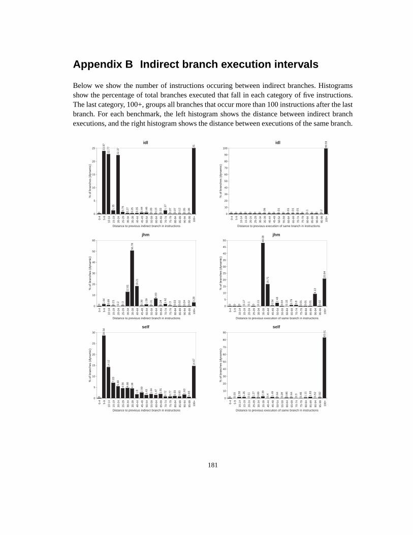
181

Appendix B Indirect branch execution intervals

Below we show the number of instructions occuring between indirect branches. Histogramsshow the percentage of total branches executed that fall in each category of five instructions.The last category, 100+, groups all branches that occur more than 100 instructions after the lastbranch. For each benchmark, the left histogram shows the distance between indirect branchexecutions, and the right histogram shows the distance between executions of the same branch.

0-4

5-9

10-

14

15-

19

20-

24

25-

29

30-

34

35-

39

40-

44

45-

49

50-

54

55-

59

60-

64

65-

69

70-

74

75-

79

80-

84

85-

89

90-

94

95-

99

100+

0

5

10

15

20

25

% o

f bra

nche

s (d

ynam

ic)

Distance to previous indirect branch in instructions

0

23.9

7

22.7

7

1.35

22.3

7

0.76

0.27

0.25

0.35

0.44

0.46

0.09

0.15

0.03 1.

37

0.07

0.07

0.12

0.05

0.06

25

idl

0-4

5-9

10-

14

15-

19

20-

24

25-

29

30-

34

35-

39

40-

44

45-

49

50-

54

55-

59

60-

64

65-

69

70-

74

75-

79

80-

84

85-

89

90-

94

95-

99

100+

0

10

20

30

40

50

60

% o

f bra

nche

s (d

ynam

ic)

Distance to previous indirect branch in instructions

0

1.64

0.89

0.21

0.2

0.3

12.8

1

50.7

8

18.2

1

0.39 1.59

0.31

6.83

0.24 1.

92

0.3

0.03

0.02

0.04

0.02 3.

28

jhm

0-4

5-9

10-

14

15-

19

20-

24

25-

29

30-

34

35-

39

40-

44

45-

49

50-

54

55-

59

60-

64

65-

69

70-

74

75-

79

80-

84

85-

89

90-

94

95-

99

100+

0

5

10

15

20

25

30

% o

f bra

nche

s (d

ynam

ic)

Distance to previous indirect branch in instructions

0

28.5

4

14.1

2

7.03

5.48

4.56

4.66

4.38

1.8 2.

59

1.43 1.84

1.47 1.91

0.72

0.77

0.93

0.83 1.

63

0.65

14.6

7

self

0-4

5-9

10-

14

15-

19

20-

24

25-

29

30-

34

35-

39

40-

44

45-

49

50-

54

55-

59

60-

64

65-

69

70-

74

75-

79

80-

84

85-

89

90-

94

95-

99

100+

0

10

20

30

40

50

60

70

80

90

100

% o

f bra

nche

s (d

ynam

ic)

Distance to previous execution of same branch in instructions

0 0 0 0 0 0 0 0.06

0 0 0.01

0 0.01

0.01

0.01

0 0.1

0 0 0.2

99.5

9idl

0-4

5-9

10-

14

15-

19

20-

24

25-

29

30-

34

35-

39

40-

44

45-

49

50-

54

55-

59

60-

64

65-

69

70-

74

75-

79

80-

84

85-

89

90-

94

95-

99

100+

0

5

10

15

20

25

30

35

40

45

50

% o

f bra

nche

s (d

ynam

ic)

Distance to previous execution of same branch in instructions

0 0 0 0.17

0.1

0 0.11

48.0

8

16.7

1

0.54 2.

48

0.04

0.15 0.79

0.8

0.01

0.01

0.01

9.13

0.02

20.8

4

jhm 0

-4

5-9

10-

14

15-

19

20-

24

25-

29

30-

34

35-

39

40-

44

45-

49

50-

54

55-

59

60-

64

65-

69

70-

74

75-

79

80-

84

85-

89

90-

94

95-

99

100+

0

10

20

30

40

50

60

70

80

90

% o

f bra

nche

s (d

ynam

ic)

Distance to previous execution of same branch in instructions

0 0.03 1.58

1.35

0.11 1.27

0.89 2.39

0.4 1.49

0.64

0.28

0.86

0.64

0.3

0.46

1.11

1.83

0.52

0.82

83.0

1self

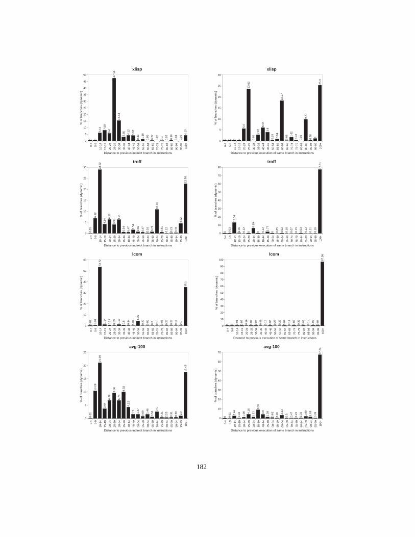
182

0-4

5-9

10-

14

15-

19

20-

24

25-

29

30-

34

35-

39

40-

44

45-

49

50-

54

55-

59

60-

64

65-

69

70-

74

75-

79

80-

84

85-

89

90-

94

95-

99

100+

0

5

10

15

20

25

30

35

40

45

50

% o

f bra

nche

s (d

ynam

ic)

Distance to previous indirect branch in instructions

0 0

6.11 7.

98

5.6

47.5

4

15.3

4

2.85 4.

12

3.92

0.31 1.18

0.05

0.27

0.02

0.1

0.02

0.39

0.04

0.02

4.13

xlisp

0-4

5-9

10-

14

15-

19

20-

24

25-

29

30-

34

35-

39

40-

44

45-

49

50-

54

55-

59

60-

64

65-

69

70-

74

75-

79

80-

84

85-

89

90-

94

95-

99

100+

0

5

10

15

20

25

30

% o

f bra

nche

s (d

ynam

ic)

Distance to previous indirect branch in instructions

0.05

6.82

28.9

2

4.14

6.26

3.95

6.2

0.54

0.47 1.

54

0.69

0.47

0.16 0.72

10.8

1

0.51

0.12

0.21

0.31

4.52

22.5

8

troff

0-4

5-9

10-

14

15-

19

20-

24

25-

29

30-

34

35-

39

40-

44

45-

49

50-

54

55-

59

60-

64

65-

69

70-

74

75-

79

80-

84

85-

89

90-

94

95-

99

100+

0

10

20

30

40

50

60

% o

f bra

nche

s (d

ynam

ic)

Distance to previous indirect branch in instructions

0.02

0.68

53.7

2

1.14

0.63

0.39 1.17

0.8

0.34

0.09

4.35

0.27

0.09

0.2

0.13

0.08

0.23

0.27

0.19

0.1

35.1

lcom

0-4

5-9

10-

14

15-

19

20-

24

25-

29

30-

34

35-

39

40-

44

45-

49

50-

54

55-

59

60-

64

65-

69

70-

74

75-

79

80-

84

85-

89

90-

94

95-

99

100+

0

5

10

15

20

25

% o

f bra

nche

s (d

ynam

ic)

Distance to previous indirect branch in instructions

0.01

10.2

8

21.0

9

3.64

6.76

9.58

6.74

9.93

4.22

1.5

1.47

0.69 1.

46

0.56

2.5

0.31

0.23

0.31

0.38 0.9

17.4

6

avg-100

0-4

5-9

10-

14

15-

19

20-

24

25-

29

30-

34

35-

39

40-

44

45-

49

50-

54

55-

59

60-

64

65-

69

70-

74

75-

79

80-

84

85-

89

90-

94

95-

99

100+

0

5

10

15

20

25

30

% o

f bra

nche

s (d

ynam

ic)

Distance to previous execution of same branch in instructions

0 0 0 0

5.6

23.6

2

0.01

2.81

6.04

3.9

0.33 0.94

18.2

7

0.08 1.

62

0.42

0.01

9.77

0.28 1

25.3

xlisp

0-4

5-9

10-

14

15-

19

20-

24

25-

29

30-

34

35-

39

40-

44

45-

49

50-

54

55-

59

60-

64

65-

69

70-

74

75-

79

80-

84

85-

89

90-

94

95-

99

100+

0

10

20

30

40

50

60

70

80

% o

f bra

nche

s (d

ynam

ic)

Distance to previous execution of same branch in instructions

0 0.03

13.0

4

0.45

0.12

0

6.19

0 0.12 1.77

0 0.05

0.02

0.16

0.07

0.15

0.03

0.12

0.11

0.26

77.3

1troff

0-4

5-9

10-

14

15-

19

20-

24

25-

29

30-

34

35-

39

40-

44

45-

49

50-

54

55-

59

60-

64

65-

69

70-

74

75-

79

80-

84

85-

89

90-

94

95-

99

100+

0

10

20

30

40

50

60

70

80

90

100

% o

f bra

nche

s (d

ynam

ic)

Distance to previous execution of same branch in instructions

0 0 0.01

0.02

0.56

0.07

0.04

0.49

0.13

0.06

0.26

0.22

0.04

0.11

0.02

0.33

0.09

0.12

0.02

0.04

97.3

6lcom

0-4

5-9

10-

14

15-

19

20-

24

25-

29

30-

34

35-

39

40-

44

45-

49

50-

54

55-

59

60-

64

65-

69

70-

74

75-

79

80-

84

85-

89

90-

94

95-

99

100+

0

10

20

30

40

50

60

70

% o

f bra

nche

s (d

ynam

ic)

Distance to previous execution of same branch in instructions

0 0.01 2.

44

0.33 1.08 4.

16

1.21

8.97

3.9

1.29

0.62

0.26 3.

23

0.3

0.47

0.23

0.23 1.

98

1.68

0.39

67.2

4avg-100

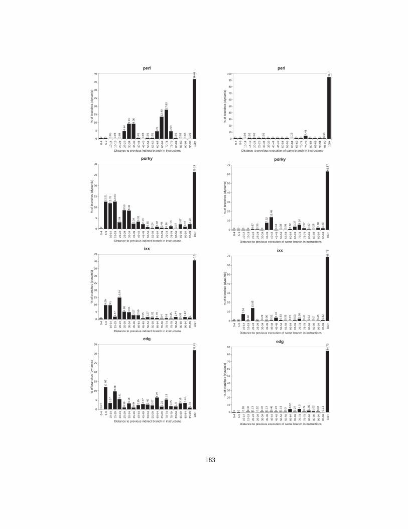
183

0-4

5-9

10-

14

15-

19

20-

24

25-

29

30-

34

35-

39

40-

44

45-

49

50-

54

55-

59

60-

64

65-

69

70-

74

75-

79

80-

84

85-

89

90-

94

95-

99

100+

0

5

10

15

20

25

30

35

40

% o

f bra

nche

s (d

ynam

ic)

Distance to previous indirect branch in instructions

0 0 0.05

0.03

0.04

4.64

9.01

9.06

0.01

0.03

0.01

0.01

4.5

13.4

9

17.8

3

4.53

0.01

0.02

0.03

0.02

36.6

8

perl

0-4

5-9

10-

14

15-

19

20-

24

25-

29

30-

34

35-

39

40-

44

45-

49

50-

54

55-

59

60-

64

65-

69

70-

74

75-

79

80-

84

85-

89

90-

94

95-

99

100+

0

5

10

15

20

25

30

% o

f bra

nche

s (d

ynam

ic)

Distance to previous indirect branch in instructions

0

12.5

1

11.7

8

12.5

3

2.94

8.53

8.42

2.34 3.

32

2.13

0.85

0.24 0.

92

0.49

0.36 1.

13

0.07

2.07

0.97 2.

18

26.2

1

porky

0-4

5-9

10-

14

15-

19

20-

24

25-

29

30-

34

35-

39

40-

44

45-

49

50-

54

55-

59

60-

64

65-

69

70-

74

75-

79

80-

84

85-

89

90-

94

95-

99

100+

0

5

10

15

20

25

30

35

40

45

% o

f bra

nche

s (d

ynam

ic)

Distance to previous indirect branch in instructions

0

9.59

9.5

1.47

14.8

4

4.98

4.64

2.57

2.55

0.55 1.27

1.02

0.78

0.4

0.6

0.45 1.44

0.33 1.

43

1

40.6

ixx

0-4

5-9

10-

14

15-

19

20-

24

25-

29

30-

34

35-

39

40-

44

45-

49

50-

54

55-

59

60-

64

65-

69

70-

74

75-

79

80-

84

85-

89

90-

94

95-

99

100+

0

5

10

15

20

25

30

35

% o

f bra

nche

s (d

ynam

ic)

Distance to previous indirect branch in instructions

0.04

11.9

2

3.37

9.68

5.41

0.99

3.18

0.94 2.

15 2.77

2.46

2.07

6.25

1.31

5.13

1.65

1.5 3.

15

3.45

0.78

31.8

1

edg

0-4

5-9

10-

14

15-

19

20-

24

25-

29

30-

34

35-

39

40-

44

45-

49

50-

54

55-

59

60-

64

65-

69

70-

74

75-

79

80-

84

85-

89

90-

94

95-

99

100+

0

10

20

30

40

50

60

70

80

90

100

% o

f bra

nche

s (d

ynam

ic)

Distance to previous execution of same branch in instructions

0 0 0.05

0.02

0.02

0 0.01

0 0 0 0 0 0.13

0 0

4.49

0 0 0 0.56

94.7

perl

0-4

5-9

10-

14

15-

19

20-

24

25-

29

30-

34

35-

39

40-

44

45-

49

50-

54

55-

59

60-

64

65-

69

70-

74

75-

79

80-

84

85-

89

90-

94

95-

99

100+

0

10

20

30

40

50

60

70

% o

f bra

nche

s (d

ynam

ic)

Distance to previous execution of same branch in instructions

0 0 0 0 0.67

0.36

0

7.32

13.4

8

0.04

0.08

0.06 0.82 3.

37 5.24

1.57

0.42

0.25 1.

98

1.48

62.8

7

porky

0-4

5-9

10-

14

15-

19

20-

24

25-

29

30-

34

35-

39

40-

44

45-

49

50-

54

55-

59

60-

64

65-

69

70-

74

75-

79

80-

84

85-

89

90-

94

95-

99

100+

0

10

20

30

40

50

60

70

% o

f bra

nche

s (d

ynam

ic)

Distance to previous execution of same branch in instructions

0 0

7.34

0.02

13.8

5

0 0.29

0.06

0.51 3.

19

0.93

0.33

0.15

0.53 2.09

0.41

0.12

0.2

0.43

0.82

68.7

3ixx

0-4

5-9

10-

14

15-

19

20-

24

25-

29

30-

34

35-

39

40-

44

45-

49

50-

54

55-

59

60-

64

65-

69

70-

74

75-

79

80-

84

85-

89

90-

94

95-

99

100+

0

10

20

30

40

50

60

70

80

90

% o

f bra

nche

s (d

ynam

ic)

Distance to previous execution of same branch in instructions

0 0 0.09

0.47

0.13

0.02

0.37

0.13

0.46

0.24

0.14

0.3 4.

02

0.27 4.

3

0.74 1.86

1.02

0.61

0.11

84.7

3

edg

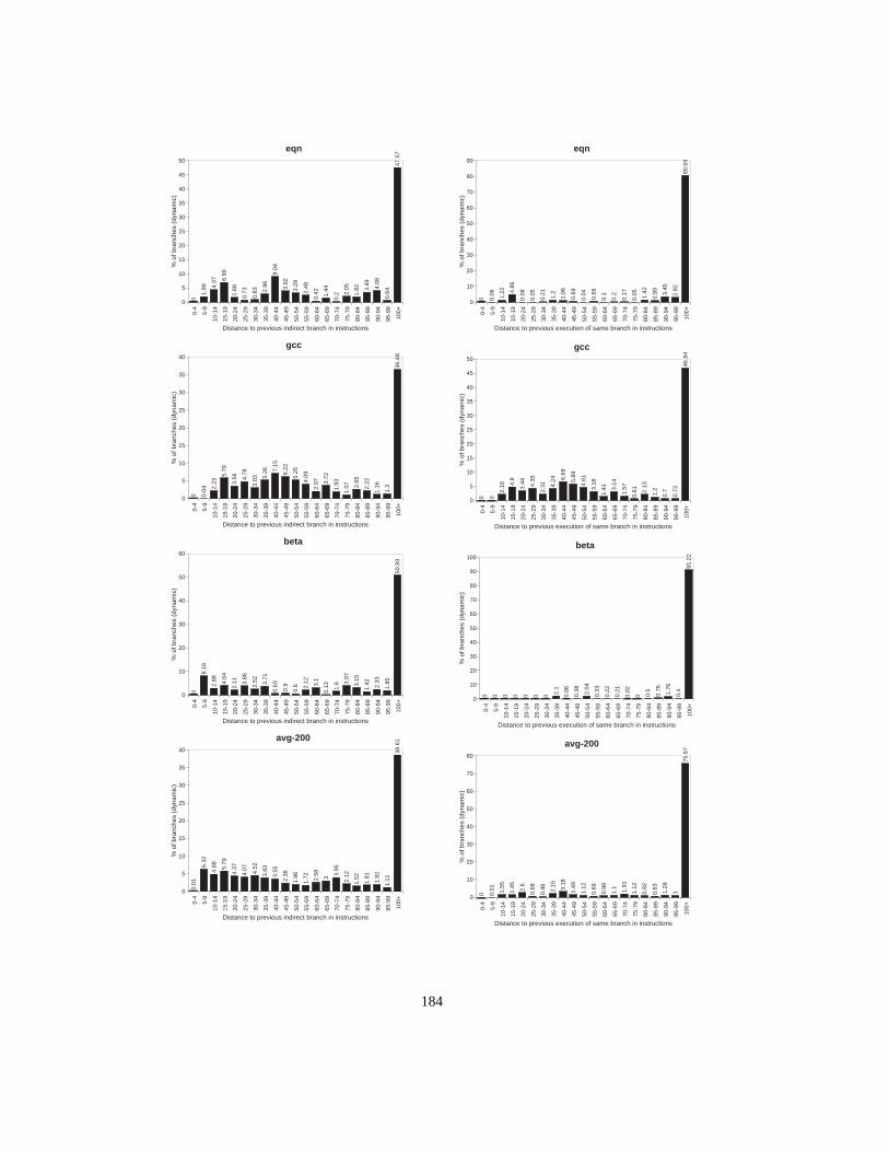
184

0-4

5-9

10-

14

15-

19

20-

24

25-

29

30-

34

35-

39

40-

44

45-

49

50-

54

55-

59

60-

64

65-

69

70-

74

75-

79

80-

84

85-

89

90-

94

95-

99

100+

0

5

10

15

20

25

30

35

40

45

50

% o

f bra

nche

s (d

ynam

ic)

Distance to previous indirect branch in instructions

0

1.99 4.

37 6.99

1.68

0.73

0.83 2.

96

9.04

3.92

3.29

2.48

0.42 1.44

0.2 2.

05

1.82 3.

49 4.08

0.64

47.5

7eqn

0-4

5-9

10-

14

15-

19

20-

24

25-

29

30-

34

35-

39

40-

44

45-

49

50-

54

55-

59

60-

64

65-

69

70-

74

75-

79

80-

84

85-

89

90-

94

95-

99

100+

0

5

10

15

20

25

30

35

40

% o

f bra

nche

s (d

ynam

ic)

Distance to previous indirect branch in instructions

0 0.04 2.

23

5.79

3.56 4.

78

3.03 5.

26 7.15

6.22

5.25

4.09

2.07 3.

72

1.93

1.07 2.

65

2.22

1.16

1.3

36.4

8

gcc

0-4

5-9

10-

14

15-

19

20-

24

25-

29

30-

34

35-

39

40-

44

45-

49

50-

54

55-

59

60-

64

65-

69

70-

74

75-

79

80-

84

85-

89

90-

94

95-

99

100+

0

10

20

30

40

50

60

% o

f bra

nche

s (d

ynam

ic)

Distance to previous indirect branch in instructions

0

8.16

2.88 4.04

2.11 3.

86

2.52 3.71

0.63

0.9

0.6 2.

12 3.1

0.13 1.

6 3.97

3.15

1.42 2.33

1.85

50.9

3

beta

0-4

5-9

10-

14

15-

19

20-

24

25-

29

30-

34

35-

39

40-

44

45-

49

50-

54

55-

59

60-

64

65-

69

70-

74

75-

79

80-

84

85-

89

90-

94

95-

99

100+

0

5

10

15

20

25

30

35

40

% o

f bra

nche

s (d

ynam

ic)

Distance to previous indirect branch in instructions

0.01

6.32

4.88 5.79

4.37

4.07 4.52

3.83

3.55

2.36

1.96

1.72 2.58 3 3.

95

2.12

1.52

1.81

1.92

1.11

38.6

1avg-200

0-4

5-9

10-

14

15-

19

20-

24

25-

29

30-

34

35-

39

40-

44

45-

49

50-

54

55-

59

60-

64

65-

69

70-

74

75-

79

80-

84

85-

89

90-

94

95-

99

100+

0

10

20

30

40

50

60

70

80

90

% o

f bra

nche

s (d

ynam

ic)

Distance to previous execution of same branch in instructions

0 0.06 1.22 4.

86

0.08

0.05

0.21 1.2

1.06

0.69

0.04

0.66

0.1

0.2

0.17

0.05 1.42

0.99 3.

45

2.92

80.5

9

eqn

0-4

5-9

10-

14

15-

19

20-

24

25-

29

30-

34

35-

39

40-

44

45-

49

50-

54

55-

59

60-

64

65-

69

70-

74

75-

79

80-

84

85-

89

90-

94

95-

99

100+

0

5

10

15

20

25

30

35

40

45

50

% o

f bra

nche

s (d

ynam

ic)

Distance to previous execution of same branch in instructions

0 0

2.18 4.

8

3.44 4.35

2.31 4.

24 6.68

5.89

4.61

3.18

1.41 3.

14

1.57

0.61 2.

13

1.2

0.7

0.73

46.8

4

gcc

0-4

5-9

10-

14

15-

19

20-

24

25-

29

30-

34

35-

39

40-

44

45-

49

50-

54

55-

59

60-

64

65-

69

70-

74

75-

79

80-

84

85-

89

90-

94

95-

99

100+

0

10

20

30

40

50

60

70

80

90

100

% o

f bra

nche

s (d

ynam

ic)

Distance to previous execution of same branch in instructions

0 0 0 0 0 0 0 2.1

0.06

0.38 2.04

0.33

0.22

0.21

0.02

0 0.5

0.76 1.76

0.4

91.2

2

beta

0-4

5-9

10-

14

15-

19

20-

24

25-

29

30-

34

35-

39

40-

44

45-

49

50-

54

55-

59

60-

64

65-

69

70-

74

75-

79

80-

84

85-

89

90-

94

95-

99

100+

0

10

20

30

40

50

60

70

80

% o

f bra

nche

s (d

ynam

ic)

Distance to previous execution of same branch in instructions

0 0.01 1.55

1.45 2.6

0.68

0.46 2.15 3.18

1.49

1.12

0.69

0.98

1.1

1.91

1.12

0.92

0.63

1.28

1

75.6

7

avg-200

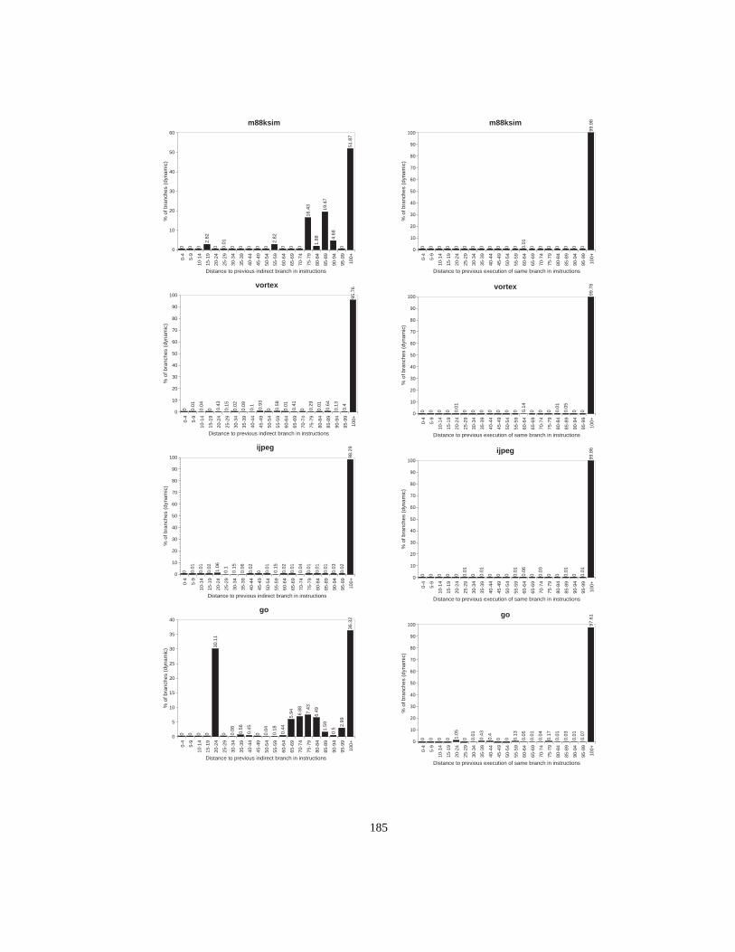
185

0-4

5-9

10-

14

15-

19

20-

24

25-

29

30-

34

35-

39

40-

44

45-

49

50-

54

55-

59

60-

64

65-

69

70-

74

75-

79

80-

84

85-

89

90-

94

95-

99

100+

0

10

20

30

40

50

60

% o

f bra

nche

s (d

ynam

ic)

Distance to previous indirect branch in instructions

0 0 0

2.82

0 0.01

0 0 0 0 0

2.82

0 0 0

16.4

3

1.88

19.4

7

4.68

0

51.8

7

m88ksim

0-4

5-9

10-

14

15-

19

20-

24

25-

29

30-

34

35-

39

40-

44

45-

49

50-

54

55-

59

60-

64

65-

69

70-

74

75-

79

80-

84

85-

89

90-

94

95-

99

100+

0

10

20

30

40

50

60

70

80

90

100

% o

f bra

nche

s (d

ynam

ic)

Distance to previous indirect branch in instructions

0 0.01

0.04

0 0.43

0.15

0.02

0.09

0.1

0.93

0 0.58

0.01

0.41

0 0.29

0.01

0.64

0.13

0.4

95.7

6vortex

0-4

5-9

10-

14

15-

19

20-

24

25-

29

30-

34

35-

39

40-

44

45-

49

50-

54

55-

59

60-

64

65-

69

70-

74

75-

79

80-

84

85-

89

90-

94

95-

99

100+

0

10

20

30

40

50

60

70

80

90

100

% o

f bra

nche

s (d

ynam

ic)

Distance to previous indirect branch in instructions

0 0.01

0.01

0.02

1.06

0.1

0.15

0.06

0.02

0 0.01

0.15

0.02

0.01

0.04

0.01

0.01

0.01

0.03

0.02

98.2

9ijpeg

0-4

5-9

10-

14

15-

19

20-

24

25-

29

30-

34

35-

39

40-

44

45-

49

50-

54

55-

59

60-

64

65-

69

70-

74

75-

79

80-

84

85-

89

90-

94

95-

99

100+

0

5

10

15

20

25

30

35

40

% o

f bra

nche

s (d

ynam

ic)

Distance to previous indirect branch in instructions

0 0 0 0

30.1

1

0 0.08 0.56

0.45

0 0.04

0.18

0.44

5.94 6.

88 7.43

6.49

1.59

0.5

2.99

36.3

2

go

0-4

5-9

10-

14

15-

19

20-

24

25-

29

30-

34

35-

39

40-

44

45-

49

50-

54

55-

59

60-

64

65-

69

70-

74

75-

79

80-

84

85-

89

90-

94

95-

99

100+

0

10

20

30

40

50

60

70

80

90

100

% o

f bra

nche

s (d

ynam

ic)

Distance to previous execution of same branch in instructions

0 0 0 0 0 0 0 0 0 0 0 0 0.01

0 0 0 0 0 0 0

99.9

8m88ksim

0-4

5-9

10-

14

15-

19

20-

24

25-

29

30-

34

35-

39

40-

44

45-

49

50-

54

55-

59

60-

64

65-

69

70-

74

75-

79

80-

84

85-

89

90-

94

95-

99

100+

0

10

20

30

40

50

60

70

80

90

100

% o

f bra

nche

s (d

ynam

ic)

Distance to previous execution of same branch in instructions

0 0 0 0 0.01

0 0 0 0 0 0 0 0.14

0 0 0 0.01

0.05

0 0

99.7

8vortex

0-4

5-9

10-

14

15-

19

20-

24

25-

29

30-

34

35-

39

40-

44

45-

49

50-

54

55-

59

60-

64

65-

69

70-

74

75-

79

80-

84

85-

89

90-

94

95-

99

100+

0

10

20

30

40

50

60

70

80

90

100

% o

f bra

nche

s (d

ynam

ic)

Distance to previous execution of same branch in instructions

0 0 0 0 0 0.01

0 0.01

0 0 0 0.01

0.06

0 0.03

0 0 0.01

0 0.01

99.8

6ijpeg

0-4

5-9

10-

14

15-

19

20-

24

25-

29

30-

34

35-

39

40-

44

45-

49

50-

54

55-

59

60-

64

65-

69

70-

74

75-

79

80-

84

85-

89

90-

94

95-

99

100+

0

10

20

30

40

50

60

70

80

90

100

% o

f bra

nche

s (d

ynam

ic)

Distance to previous execution of same branch in instructions

0 0 0 0 1.05

0 0.01

0.43

0.4

0 0 0.13

0.05

0.01

0.04

0.17

0.01

0.03

0.01

0.07

97.6

1go

186