Soft Margins for AdaBoost - Springer1007618119488.pdf · SOFT MARGINS FOR ADABOOST 289 weights c...
34
Machine Learning, 42, 287–320, 2001 c 2001 Kluwer Academic Publishers. Manufactured in The Netherlands. Soft Margins for AdaBoost G. R ¨ ATSCH [email protected] GMD FIRST, * Kekul´ estr. 7, 12489 Berlin, Germany T. ONODA [email protected] CRIEPI, † Komae-shi, 2-11-1 Iwado Kita, Tokyo, Japan K.-R. M ¨ ULLER [email protected] GMD FIRST, Kekul´ estr. 7, 12489 Berlin, Germany; University of Potsdam, * Neues Palais 10, 14469 Potsdam, Germany Editor: Robert Schapire Abstract. Recently ensemble methods like ADABOOST have been applied successfully in many problems, while seemingly defying the problems of overfitting. ADABOOST rarely overfits in the low noise regime, however, we show that it clearly does so for higher noise levels. Central to the understandingof this fact is the margin distribution. ADABOOST can be viewed as a constraint gradient descent in an error function with respect to the margin. We find that ADABOOST asymptotically achieves a hard margin distribution, i.e. the algorithm concentrates its resources on a few hard-to-learn patterns that are interestingly very similar to Support Vectors. A hard margin is clearly a sub-optimal strategy in the noisy case, and regularization, in our case a “mistrust” in the data, must be introduced in the algorithm to alleviate the distortions that single difficult patterns (e.g. outliers) can cause to the margin distribution. We propose several regularization methods and generalizations of the original ADABOOST algorithm to achieve a soft margin. In particular we suggest (1) regularized ADABOOST REG where the gradient decent is done directly with respect to the soft margin and (2) regularized linear and quadratic programming (LP/QP-) ADABOOST, where the soft margin is attained by introducing slack variables. Extensive simulations demonstrate that the proposed regularized ADABOOST-type algorithms are useful and yield competitive results for noisy data. Keywords: ADABOOST, arcing, large margin, soft margin, classification, support vectors 1. Introduction Boosting and other ensemble 1 learning methods have been recently used with great success in applications like OCR (Schwenk & Bengio, 1997; LeCun et al., 1995). But so far the reduction of the generalization error by Boosting algorithms has not been fully understood. For low noise cases Boosting algorithms are performing well for good reasons (Schapire et al., 1997; Breiman, 1998). However, recent studies with highly noisy patterns (Quinlan, 1996; Grove & Schuurmans, 1998; R¨ atsch et al., 1998) showed that it is clearly a myth that Boosting methods do not overfit. * www.first.gmd.de † criepi.denken.or.jp * www.uni-potsdam.de
-
Upload
truongthuan -
Category
Documents
-
view
219 -
download
1
Transcript of Soft Margins for AdaBoost - Springer1007618119488.pdf · SOFT MARGINS FOR ADABOOST 289 weights c...

Machine Learning, 42, 287–320, 2001c© 2001 Kluwer Academic Publishers. Manufactured in The Netherlands.
Soft Margins for AdaBoost
G. RATSCH [email protected] FIRST,∗ Kekulestr. 7, 12489 Berlin, Germany
T. ONODA [email protected],† Komae-shi, 2-11-1 Iwado Kita, Tokyo, Japan
K.-R. MULLER [email protected] FIRST, Kekulestr. 7, 12489 Berlin, Germany; University of Potsdam,∗ Neues Palais 10,14469 Potsdam, Germany
Editor: Robert Schapire
Abstract. Recently ensemble methods like ADABOOST have been applied successfully in many problems,while seemingly defying the problems of overfitting.
ADABOOST rarely overfits in the low noise regime, however, we show that it clearly does so for higher noiselevels. Central to the understanding of this fact is the margin distribution. ADABOOST can be viewed as a constraintgradient descent in an error function with respect to the margin. We find that ADABOOST asymptotically achievesa hard margindistribution, i.e. the algorithm concentrates its resources on a few hard-to-learn patterns that areinterestingly very similar to Support Vectors. A hard margin is clearly a sub-optimal strategy in the noisy case, andregularization, in our case a “mistrust” in the data, must be introduced in the algorithm to alleviate the distortionsthat single difficult patterns (e.g. outliers) can cause to the margin distribution. We propose several regularizationmethods and generalizations of the original ADABOOST algorithm to achieve asoft margin. In particular wesuggest (1) regularized ADABOOSTREG where the gradient decent is done directly with respect to the soft marginand (2) regularized linear and quadratic programming (LP/QP-) ADABOOST, where the soft margin is attainedby introducing slack variables.
Extensive simulations demonstrate that the proposed regularized ADABOOST-type algorithms are useful andyield competitive results for noisy data.
Keywords: ADABOOST, arcing, large margin, soft margin, classification, support vectors
1. Introduction
Boosting and other ensemble1 learning methods have been recently used with great successin applications like OCR (Schwenk & Bengio, 1997; LeCun et al., 1995). But so far thereduction of the generalization error by Boosting algorithms has not been fully understood.
For low noisecases Boosting algorithms are performing well for good reasons (Schapireet al., 1997; Breiman, 1998). However, recent studies withhighly noisy patterns (Quinlan,1996; Grove & Schuurmans, 1998; R¨atsch et al., 1998) showed that it is clearly a myth thatBoosting methods do not overfit.
∗www.first.gmd.de†criepi.denken.or.jp∗www.uni-potsdam.de

288 G. RATSCH, T. ONODA AND K.-R. MULLER
In this work, we try to gain insight into these seemingly contradictory results for the lowand high noise regime and we propose improvements of ADABOOST that help to achievenoise robustness.
Due to their similarity, we will refer in the following to ADABOOST (Freund & Schapire,1994) and unnormalized Arcing(Breiman, 1997b) (with exponential function) asADABOOST-type algorithms(ATA). In Section 2 we give an asymptotical analysis of ATAs.We find that the error function of ATAs can be expressed in terms of the margin and that inevery iteration ADABOOST tries to minimize this error by a stepwise maximization of themargin (see also Breiman, 1997a; Frean & Downs, 1998; Friedman, Hastie, & Tibshirani,1998; Onoda, R¨atsch, & Muller, 1998; Ratsch, 1998). As a result of the asymptotical anal-ysis of this error function, we introduce thehard marginconcept and show connections toSupport Vector (SV) learning (Boser, Guyon, & Vapnik, 1992) and to linear programming(LP). Bounds on the size of the margin are also given.
In Section 3 we explain why an ATA that enforces a hard margin in training will overfitfor noisy data or overlapping class distributions. So far, we only know what a margin distri-bution to achieve optimal classification in the no-noise case should look like: a large hardmargin is clearly a good choice (Vapnik, 1995). However, for noisy data there is always thetradeoff between “believing” in the data or “mistrusting” it, as the very data point couldbe mislabeled or an outlier. So we propose to relax the hard margin and to regularize byallowing for misclassifications (soft margin). In Section 4 we introduce such a regulariza-tion strategy to ADABOOST and subsequently extend the LP-ADABOOST algorithm ofGrove and Schuurmans (1998) by slack variables to achieve soft margins. Furthermore, wepropose a quadratic programming ADABOOST algorithm (QP-ADABOOST) and show itsconnections to SUPPORTVECTORMACHINES (SVMs).
Finally, in Section 5 numerical experiments on several artificial and real-world data setsshow the validity and competitiveness of our regularized Boosting algorithms. The paperconcludes with a brief discussion.
2. Analysis of ADABOOST’s learning process
2.1. Algorithm
Let {ht (x) : t = 1, . . . , T} be an ensemble ofT hypotheses defined on an input vectorx ∈ X and letc = [c1 · · · cT ] be their weights satisfyingct ≥ 0 and
∑Tt=1 ct = 1. We
will consider only the binary classification case in this work, i.e.ht (x) = ±1; most results,however, can be transfered easily to classification with more than two classes (e.g. Schapire,1999; Schapire & Singer, 1998; Breiman, 1997b).
The ensemble generates the labelf (x) ≡ fT (x) which is the weighted majority of thevotes, where
fT (x) :=T∑
t=1
ctht (x) and fT (x) := sign( fT (x)).
In order to train the ensemble, i.e. to findT appropriate hypotheses{ht (x)} and the
SOFT MARGINS FOR ADABOOST 289
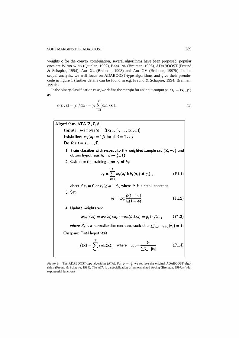
weightsc for the convex combination, several algorithms have been proposed: popularones are WINDOWING (Quinlan, 1992), BAGGING (Breiman, 1996), ADABOOST (Freund& Schapire, 1994), ARC-X4 (Breiman, 1998) and ARC-GV (Breiman, 1997b). In thesequel analysis, we will focus on ADABOOST-type algorithms and give their pseudo-code in figure 1 (further details can be found in e.g. Freund & Schapire, 1994; Breiman,1997b).
In the binary classification case, we define themarginfor an input-output pairzi = (xi , yi )
as
ρ(zi , c) = yi f (xi ) = yi
T∑t=1
cthr (xi ), (1)
Figure 1. The ADABOOST-type algorithm (ATA). Forφ = 12 , we retrieve the original ADABOOST algo-
rithm (Freund & Schapire, 1994). The ATA is a specialization of unnormalized Arcing (Breiman, 1997a) (withexponential function).
290 G. RATSCH, T. ONODA AND K.-R. MULLER
wherei = 1, . . . , l andl denotes the number of training patterns. The margin atz is positiveif the correct class label of the pattern is predicted. As the positivity of the margin valueincreases, the decision stability becomes larger. Moreover, if|c| := ∑T
t=1 ct = 1, thenρ(zi , c) ∈ [−1, 1]. We will sometimes for convenience also use a margin definition withb (instead ofc) which denotes simply an unnormalized version ofc, i.e. usually|b| 6= 1(cf. (F1.2) and (F1.4) in figure 1). Note that theedge(cf. Breiman, 1997b) is just an affinetransformation of the margin.
The margin%(c) of a classifier (instance) is defined as the smallest margin of a patternover the training set, i.e.
%(c) = mini=1,...,l
ρ(zi , c).
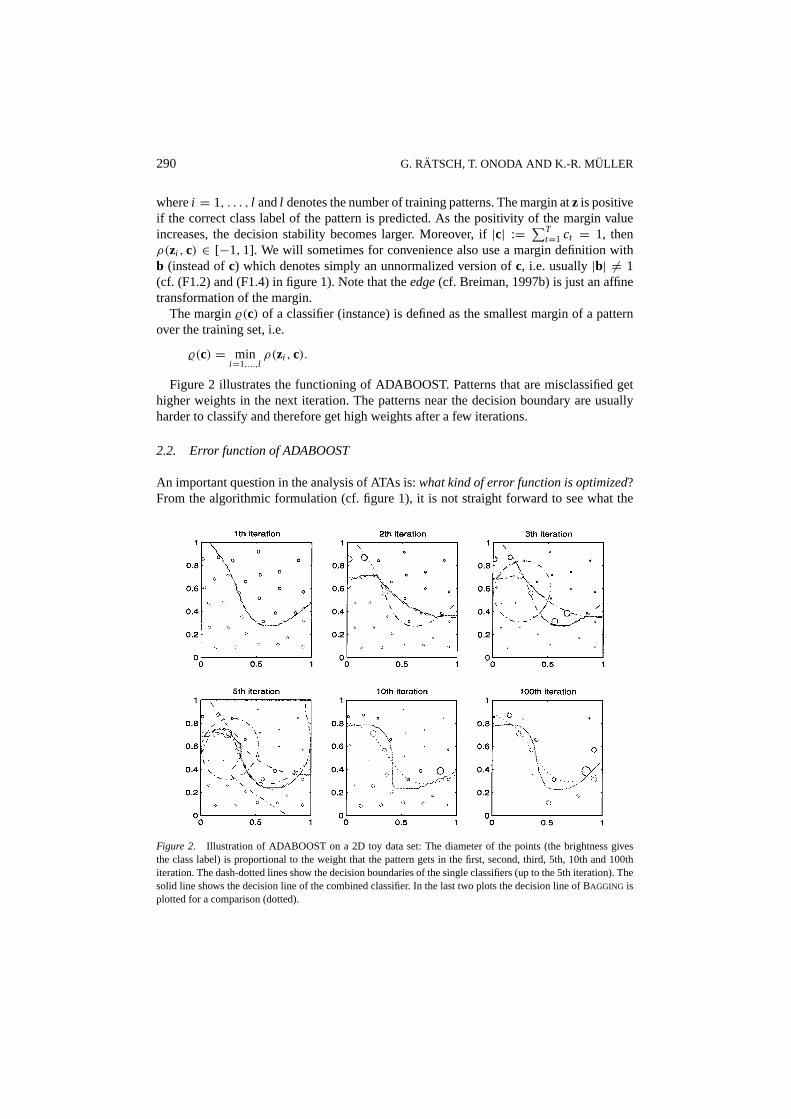
Figure 2 illustrates the functioning of ADABOOST. Patterns that are misclassified gethigher weights in the next iteration. The patterns near the decision boundary are usuallyharder to classify and therefore get high weights after a few iterations.
2.2. Error function of ADABOOST
An important question in the analysis of ATAs is:what kind of error function is optimized?From the algorithmic formulation (cf. figure 1), it is not straight forward to see what the
Figure 2. Illustration of ADABOOST on a 2D toy data set: The diameter of the points (the brightness givesthe class label) is proportional to the weight that the pattern gets in the first, second, third, 5th, 10th and 100thiteration. The dash-dotted lines show the decision boundaries of the single classifiers (up to the 5th iteration). Thesolid line shows the decision line of the combined classifier. In the last two plots the decision line of BAGGING isplotted for a comparison (dotted).

SOFT MARGINS FOR ADABOOST 291
aim of this algorithm is. So to gain a better understanding why one should use the weightsof the hypothesesct and of the patternswt (zi ) in the manner of Eqs. (F1.2) and (F1.3), letus study the following three statements
1. The weightswt (zi ) in thet-th iteration are chosen such that the previous hypothesis hasexactly a weighted training errorε of 1/2 (Schapire et al., 1997).
2. The weightbt (andct ) of a hypothesis is chosen such that it minimizes a functionalGfirst introduced by Breiman (1997b) (see also R¨atsch, 1998; Mason, Bartlett, & Baxter,2000a; Onoda et al., 1998; Friedman et al., 1998; Frean & Downs, 1998). This functionaldepends on the margins of all patterns and is defined by
G(bt , bt−1) =l∑
i=1
exp
{−ρ(zi , bt )+ |bt |
(1
2− φ
)}, (2)
whereφ is a constant (cf. figure 1). This functional can be minimized analytically(Breiman, 1997b) and one gets the explicit form of Eq. (F1.2) as a solution of∂G(bt ,bt−1)
∂bt= 0.
3. To train thet-th hypothesis (step 1 in figure 1) we can either use bootstrap replicatesof the training set (sampled according towt ) or minimize a weighted error function forthe base learning algorithm. We observed that the convergence of the ATA is faster if aweighted error function is used.
Taking a closer look at the definition ofG, one finds that the computation of the sampledistributionwt (cf. Eq. (F1.3)) can be derived directly fromG. Assuming thatG is the errorfunction which is minimized by the ATA, thenG essentially defines a loss function overmargin distributions, which depends on the value of|b|. The larger the marginsρ(zi ), thesmaller will be the value ofG.
So, the gradient ∂G∂ρ(zi )
gives an answer to the question, which pattern should increase itsmargin most strongly in order to decreaseG maximally (gradient descent). This informationcan then be used to compute a re-weighting of the sample distributionwt for training the nexthypothesisht . If it is important to increase the margin of a patternzi , then its weightwt (zi )
should be high—otherwise low (because the distributionwt sums to one). Interestingly, thisis exactly what ATAs are doing and we arrive at the following lemma (Breiman, 1997b;Ratsch, 1998):
Lemma 1. The computation of the pattern distributionwt+1 in the t-th iteration is equiv-alent to normalizing the gradient of G(bt+1, bt ) with respect toρ(zi , bt ), i.e.
wt+1(zi ) = ∂G(bt+1, bt )
∂ρ(zi , bt )
/l∑
j=1
∂G(bt+1, bt )
∂ρ(z j , bt ). (3)
The proof can found in Appendix A.From Lemma 1, the analogy to a gradient descent method is (almost) complete. In a
gradient descent method, the first step is to compute the gradient of the error function with
292 G. RATSCH, T. ONODA AND K.-R. MULLER
respect to the parameters which are to be optimized: this corresponds to computing thegradient ofG with respect to the margins. The second step is to determine the step size ingradient direction (usually done by a line-search): this is analogous to the minimization ofG with respect tobt (cf. point 2).
Therefore, ATAs can be related to a gradient descent method in a hypothesis (or function)spaceH which is determined by the structure of the base learning algorithm, i.e. ATAs aimto minimize the functionalG by constructing an ensemble of classifiers (Onoda et al.,1998; Ratsch, 1998; Mason et al., 2000b; Friedman et al., 1998; Friedman, 1999). This alsoexplains point 1 in the list above, as in a standard gradient descent method, a new searchdirection is usually chosen perpendicular to the previous one.
In the ADABOOST-type algorithm, the gradients are found by changing the weights ofthe training patterns, and there are essentially two ways of incorporating the re-weightinginto the boosting procedure. The first is to create bootstrap replicates sampled according tothe pattern weightings, which usually induces strong random effects that hide the “true” in-formation contained in the pattern weightings. The second and more direct way is to weightthe error function and use weighted minimization (Breiman, 1997b). Clearly, weightedminimization is more efficient in terms of the number of boosting iterations than the boot-strap approach.2 In fact, it can be shown that employing weighted minimization (Breiman,1997b) for finding the next hypothesis in each iteration leads to the best (single) hypothesisfor minimizing G (Mason et al., 2000a), i.e. adding the hypothesis with smallest weightedtraining errorεt will lead to the smallest value ofG and therefore to a fast convergence.This reasoning explains the third statement.
2.3. ADABOOST as an annealing process
From the definition ofG andρ(zi , bt ), Eq. (3) can be rewritten as
wt+1(zi ) =exp
(− 12ρ(zi , ct )
)|bt |∑lj=1 exp
(− 12ρ(z j , ct )
)|bt | , (4)
where we emphasize that|bt | can be written in the exponent. Inspecting this equation moreclosely, we see that ATA uses a soft-max function (e.g. Bishop, 1995) with parameter|bt |that we would like to interpret as anannealing parameter(Onoda et al., 1998; Onoda,Ratsch, & Muller, 2000). In the beginning|bt | is small and all patterns have almost thesame weights (if|bt | = 0 then all weights are the same). As|bt | increases, the patternswith smallest margin will get higher and higher weights. In the limit of large|bt |, we arriveat the maximum function: Only the pattern(s) with the smallest margin will be taken intoaccount for learning and get a non-zero weight.
Note that in the limit for|bt | → ∞, a simple rescaling of the error functionG(bt ) givesthe minimum margin%(zi , ct ), i.e.%(zi , ct ) = −lim|bt |→∞ 1
|bt | logG(bt ).The following lemma shows that under usual circumstances, the length of the hypothesis
weight vector|bt | increases at least linearly with the number of iterations.

SOFT MARGINS FOR ADABOOST 293
Lemma 2. If, in the learning process of an ATA with0 < φ < 1, all weighted trainingerrorsεt are bounded byεt ≤ φ−1 (0< 1 < φ), then|b| increases at least linearly withthe number of iterations t.
Proof: With (F1.2), the smallest value forbt is achieved, ifεt = φ − 1. Then wehavebt = log q
q−1 , whereq := φ(1 − φ + 1). We find q > 1 > 0 and because ofφ(1− φ) > 1(1− φ) we getφ(1− φ +1) > 1 and hence alsoq −1 > 0. Therefore,the smallest value ofbt is log q
q−1 is always larger than a constantγ , which only dependsonφ and1. Thus, we have|bt | > tγ . 2
If the annealing speed is low, the achieved solution should have larger margins than fora high speed annealing strategy. This holds for similar reasons as for a standard annealingprocess (Kirkpatrick, 1984): in the error surface, a better local minimum (if exist) can beobtained locally, if the annealing speed is slow enough. From Eq. (F1.2), we observe thatif the training errorεt takes a small value,bt becomes large. So, strong learners can reducetheir training errors strongly and will make|b| large after only a few ATA iterations, i.e.the asymptotics, where the addition of a new ensemble member does not change the result,is reached faster. To reduce the annealing speed eitherφ or the complexity of the basehypotheses has to be decreased (with the constraintεt < φ −1; cf. Onoda et al., 1998).
In figure 3 (left), the ADABOOST Error (φ = 12), the Squared Error(y− f (x))2 and the
Kullback-Leibler Error lnρ(z)/ln 2 are plotted. Interestingly, the Squared and Kullback-Leibler Error are very similar to the error function of ADABOOST for|b| = 3. As |b|increases,3 the ATA error function approximates a 0/∞ loss (patterns with margin smallerthan 1−2φ get loss∞; all others have loss 0) and bounds the 0/1 loss at 1−2φ from above.
Figure 3. Different loss functions for classification (see text). The abscissa shows the marginy f (x) of a patternand the y-coordinate shows the monotone loss for that pattern: 0/1-Loss, Squared Error, Kullback-Leibler Errorand ADABOOST Error (cf. Eq. (2)), where|b| is either 3, 5, 10 or 100 (in reading order). On the left panel isφ = 1/2 and on the right plotφ is either 1/3 or 2/3. The step position of the 0/∞ loss, which is approximatedfor |b| → ∞, is determined byφ.

294 G. RATSCH, T. ONODA AND K.-R. MULLER
Figure 3 (right) shows the different offsets of the step seen in the ATA Error(|b| → ∞).They result from different values ofφ (hereφ is either 1/3 or 2/3).
2.4. Asymptotic analysis
2.4.1. How large is the margin? ATA’s good generalization performance can be explainedin terms of the size of the (hard) margin that can be achieved (Schapire et al., 1997; Breiman,1997b): for low noise, the hypothesis with the largest margin will have the best generalizationperformance (Vapnik, 1995; Schapire et al., 1997). Thus, it is interesting to understand whatthe margin size depends on.
Generalizing Theorem 5 of Freund and Schapire (1994) to the caseφ 6= 12 we get
Theorem 3. Assume, ε1, . . . , εT are the weighted classification errors of h1, . . . , hT thatare generated by running an ATA and1 > φ > maxt=1, . . . ,T εt . Then the followinginequality holds for allθ ∈ [−1, 1]:
1
l
l∑i=1
I (yi f (xi ) ≤ θ) ≤(ϕ
1+θ2 + ϕ− 1−θ
2)T
T∏t=1
√ε1−θ
t (1− εt )1+θ , (5)
where f is the final hypothesis andϕ = φ
1−φ , where I is the indicator function.
The proof can be found in Appendix B.
Corollary 4. An ADABOOST-type algorithm will asymptotically(t →∞) generate mar-gin distributions with a margin%, which is bounded from below by
% ≥ ln(φε−1)+ ln((1− φ)(1− ε)−1)
ln(φε−1)− ln((1− φ)(1− ε)−1), (6)
whereε = maxt εt , if ε ≤ (1− %)/2 is satisfied.
Proof: The maximum ofε1−θt (1− εt )
1+θ with respect toεt is obtained for12(1− θ) andfor 0≤ εt ≤ 1
2(1− θ) it is increasing monotonically inεt . Therefore, we can replaceεt byε in Eq. (5) forθ ≤ %:
P(x,y)∼Z [y f (x) ≤ θ ] ≤ ((ϕ 1+θ2 + ϕ− 1−θ
2)ε
1−θ2 (1− ε) 1+θ
2)T.
If the basis on the right hand side is smaller than 1, then asymptotically we haveP(x,y)∼Z
[y f (x) ≤ θ ] = 0; this means that asymptotically, there is no example that has a smallermargin thanθ , for any θ < 1. The supremum over allθ such that the basis is less than1, θmax is described by(
ϕ1+θmax
2 + ϕ− 1−θmax2)ε
1−θmax2 (1− ε) 1+θmax
2 = 1.
SOFT MARGINS FOR ADABOOST 295
We can solve this equation to obtainθmax
θmax= ln(φε−1)+ ln((1− φ)(1− ε)−1)
ln(φε−1)− ln((1− φ)(1− ε)−1).
We get the assertion because% is always larger or equalθmax. 2
From Eq. (6) we can see the interaction betweenφ andε: if the difference betweenε andφ is small, then the right hand side of (6) is small. The smallerφ is, the more importantthis difference is. From Theorem 7.2 of Breiman (1997b) we also have the weaker bound% ≥ 1− 2φ and so, ifφ is small then% must be large, i.e. choosing a smallφ results in alarger margin on the training patterns. On the other hand, an increase of the complexity ofthe basis algorithm leads to an increased%, because the errorεt will decrease.
2.4.2. Support patterns.A decrease in the functionalG(c, |b|) := G(b) (with c= b/|b|)is predominantly achieved by improvements of the marginρ(zi , c). If the marginρ(zi , c) isnegative, then the errorG(c, |b|) clearly takes a large value, amplified by|b| in the exponent.So, ATA tries to decrease the negative margins most efficiently in order to improve the errorG(c, |b|).
Now let us consider the asymptotic case, where the number of iterations and therefore|b| take large values (cf. Lemma 2). Here, the marginsρ(zi , c) of all patternsz1, . . . , zl ,are almost the same and small differences are amplified strongly inG(c, |b|). For example,given two marginsρ(zi , c) = 0.2 andρ(z j , c) = 0.3 and|b| = 100, then this difference isamplified exponentially exp{− 100×0.2
2 } = e−10 and exp{− 100×0.32 } = e−15 in G(c, |b|), i.e.
by a factor ofe5 ≈ 150. From Eq. (4) we see that as soon as the annealing parameter|b| islarge, the ATA learning becomes a hard competition case: only the patterns with smallestmargin will get high weights, other patterns are effectively neglected in the learning process.We get the following interesting lemma.
Lemma 5. During the ATA learning process, the smallest margin of the(training)patternsof each class will asymptotically converge to the same value, i.e.
limt→∞ min
i :yi=1ρ(zi , ct ) = lim
t→∞ mini :yi=−1
ρ(zi , ct ), (7)
if the following assumptions are fulfilled:
1. the weight of each hypothesis is bounded from below and above by
0< γ < bt < 0 <∞, and (8)
2. the learning algorithm must(in principle) be able to classify all patterns to one classc ∈ {±1}, if the sum over the weights of patterns of class c is larger than a constantδ,
i.e. ∑i :yi=c
w(zi ) > δ ⇒ h(xi ) = c (i = 1, . . . , l ). (9)
The proof can be found in Appendix C.
296 G. RATSCH, T. ONODA AND K.-R. MULLER
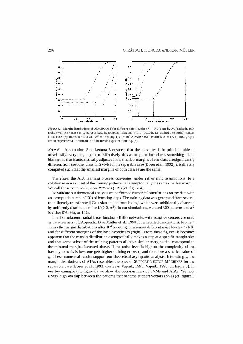
Figure 4. Margin distributions of ADABOOST for different noise levels:σ 2 = 0% (dotted), 9% (dashed), 16%(solid) with RBF nets (13 centers) as base hypotheses (left); and with 7 (dotted), 13 (dashed), 30 (solid) centersin the base hypotheses for data withσ 2 = 16% (right) after 104 ADABOOST iterations (φ = 1/2). These graphsare an experimental confirmation of the trends expected from Eq. (6).
Note 6. Assumption 2 of Lemma 5 ensures, that the classifier is in principle able tomisclassify every single pattern. Effectively, this assumption introduces something like abias termb that is automatically adjusted if the smallest margins of one class are significantlydifferent from the other class. In SVMs for the separable case (Boser et al., 1992),b is directlycomputed such that the smallest margins of both classes are the same.
Therefore, the ATA learning process converges, under rather mild assumptions, to asolution where a subset of the training patterns has asymptotically the same smallest margin.We call these patternsSupport Patterns(SPs) (cf. figure 4).
To validate our theoretical analysis we performed numerical simulations on toy data withan asymptotic number (104) of boosting steps. The training data was generated from several(non-linearly transformed) Gaussian and uniform blobs,4 which were additionally distortedby uniformly distributed noiseU (0.0, σ 2). In our simulations, we used 300 patterns andσ 2
is either 0%, 9%, or 16%.In all simulations, radial basis function (RBF) networks with adaptive centers are used
as base learners (cf. Appendix D or M¨uller et al., 1998 for a detailed description). Figure 4shows the margin distributions after 104 boosting iterations at different noise levelsσ 2 (left)and for different strengths of the base hypotheses (right). From these figures, it becomesapparent that the margin distribution asymptotically makes a step at a specific margin sizeand that some subset of the training patterns all have similar margins that correspond tothe minimal margin discussed above. If the noise level is high or the complexity of thebase hypothesis is low, one gets higher training errorsεt and therefore a smaller value of%. These numerical results support our theoretical asymptotic analysis. Interestingly, themargin distributions of ATAs resembles the ones of SUPPORTVECTORMACHINES for theseparable case (Boser et al., 1992; Cortes & Vapnik, 1995; Vapnik, 1995, cf. figure 5). Inour toy example (cf. figure 6) we show the decision lines of SVMs and ATAs. We notea very high overlap between the patterns that become support vectors (SVs) (cf. figure 6

SOFT MARGINS FOR ADABOOST 297
Figure 5. Typical margin distribution graphs (normalized) of a SVM with hard margin (solid) and soft marginwith C = 10−3 (dashed) andC = 10−1 (dash-dotted). Here for the same toy example a RBF kernel (width= 0.3)is used. The generalization error of the SVM with hard margin is more than two times larger as withC = 10−1.
Figure 6. Training patterns with decision lines for ADABOOST (left) with RBF nets (13 centers) and SVM(right) for a low noise case with similar generalization errors. The positive and negative training patterns areshown as ‘+’ and ‘∗’ respectively, the support patterns and support vectors are marked with ‘o’.
right) and the patterns that lie within the step part of the margin distribution for ATA (cf.figure 4 left).
So, the ADABOOST-type algorithm achieves asymptotically a decision withhard margin,very similar to the one of SVMs for the separable case. Intuitively this is clear: the mostdifficult patterns are emphasized strongly and become support patterns or support vectorsasymptotically. The degree of overlap between the support vectors and support patternsdepends on the kernel (SVM) and on the base hypothesis (ATA) being used. For the SUPPORT
VECTOR MACHINE with RBF kernel the highest overlap was achieved, when the averagewidths of the RBF networks was used as kernel width for the SUPPORTVECTORMACHINE

298 G. RATSCH, T. ONODA AND K.-R. MULLER
Figure 7. Typical margin distribution graphs of (original) ADABOOST after 20 (dotted), 70 (dash-dotted), 200(dashed) and 104 (solid) iterations. Here, the toy example (300 patterns,σ = 16%) and RBF networks with 30centers are used. After already 200 iterations the asymptotical convergence is almost reached.
(Ratsch, 1998). We have also observed this striking similarity of SPs in ADABOOST andSVs of the SVM in several other non-toy applications.
In the sequel, we can often assume the asymptotic case, where a hard margin is achieved(the more hypotheses we combine, the better is this approximation). Experimentally wefind that the hard margin approximation is valid (cf. Eq. (4)) already for e.g.|b| > 100.This is illustrated by figure 7, which shows some typical ATA margin distributions after 20,70, 200 and 104 iterations.To recapitulate our findings of this section:
1. ADABOOST-type algorithms aim to minimize a functional, which depends on the margindistribution. The minimization is done by means of a constraint gradient descent withrespect to the margin.
2. Some training patterns, which are in the area of the decision boundary, have asymptot-ically (for a large number of boosting steps) the same margin. We call these patternsSupport Patterns. They have a large overlap to the SVs found by a SVM.
3. Asymptotically, ATAs reach a hard margin comparable to the one obtained by the originalSVM approach (Boser et al., 1992).
4. Larger hard margins can be achieved, ifεt (more complex base hypotheses) and/orφ
are small (cf. Corollary 4). For the low noise case, a choice ofθ 6= 12 can lead to a
better generalization performance, as shown for e.g. OCR benchmark data in Onodaet al. (1998).
3. Hard margin and overfitting
In this section, we give reasons why the ATA isnot noise robustand exhibits suboptimalgeneralization ability in the presence of noise. According to our understanding, noisy datahas at least one of the following properties: (a) overlapping class probability distributions,
SOFT MARGINS FOR ADABOOST 299
(b) outliers and (c) mislabeled patterns. All three types of noise appear very often in dataanalysis. Therefore the development of a noise robust version of ADABOOST is veryimportant.
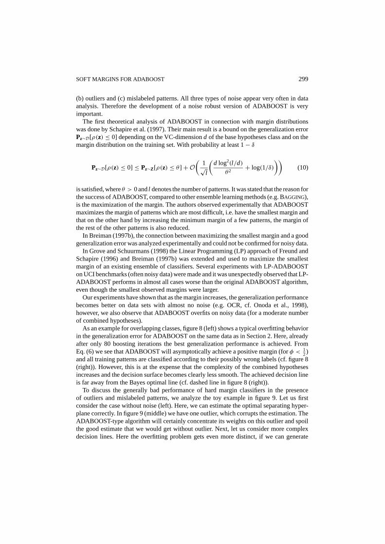
The first theoretical analysis of ADABOOST in connection with margin distributionswas done by Schapire et al. (1997). Their main result is a bound on the generalization errorPz∼D[ρ(z) ≤ 0] depending on the VC-dimensiond of the base hypotheses class and on themargin distribution on the training set. With probability at least 1− δ
Pz∼D[ρ(z) ≤ 0] ≤ Pz∼Z [ρ(z) ≤ θ ] +O(
1√l
(d log2(l/d)
θ2+ log(1/δ)
))(10)
is satisfied, whereθ > 0 andl denotes the number of patterns. It was stated that the reason forthe success of ADABOOST, compared to other ensemble learning methods (e.g. BAGGING),is the maximization of the margin. The authors observed experimentally that ADABOOSTmaximizes the margin of patterns which are most difficult, i.e. have the smallest margin andthat on the other hand by increasing the minimum margin of a few patterns, the margin ofthe rest of the other patterns is also reduced.
In Breiman (1997b), the connection between maximizing the smallest margin and a goodgeneralization error was analyzed experimentally and could not be confirmed for noisy data.
In Grove and Schuurmans (1998) the Linear Programming (LP) approach of Freund andSchapire (1996) and Breiman (1997b) was extended and used to maximize the smallestmargin of an existing ensemble of classifiers. Several experiments with LP-ADABOOSTon UCI benchmarks (often noisy data) were made and it was unexpectedly observed that LP-ADABOOST performs in almost all cases worse than the original ADABOOST algorithm,even though the smallest observed margins were larger.
Our experiments have shown that as the margin increases, the generalization performancebecomes better on data sets with almost no noise (e.g. OCR, cf. Onoda et al., 1998),however, we also observe that ADABOOST overfits on noisy data (for a moderate numberof combined hypotheses).
As an example for overlapping classes, figure 8 (left) shows a typical overfitting behaviorin the generalization error for ADABOOST on the same data as in Section 2. Here, alreadyafter only 80 boosting iterations the best generalization performance is achieved. FromEq. (6) we see that ADABOOST will asymptotically achieve a positive margin (forφ < 1
2)and all training patterns are classified according to their possibly wrong labels (cf. figure 8(right)). However, this is at the expense that the complexity of the combined hypothesesincreases and the decision surface becomes clearly less smooth. The achieved decision lineis far away from the Bayes optimal line (cf. dashed line in figure 8 (right)).
To discuss the generally bad performance of hard margin classifiers in the presenceof outliers and mislabeled patterns, we analyze the toy example in figure 9. Let us firstconsider the case without noise (left). Here, we can estimate the optimal separating hyper-plane correctly. In figure 9 (middle) we have one outlier, which corrupts the estimation. TheADABOOST-type algorithm will certainly concentrate its weights on this outlier and spoilthe good estimate that we would get without outlier. Next, let us consider more complexdecision lines. Here the overfitting problem gets even more distinct, if we can generate

300 G. RATSCH, T. ONODA AND K.-R. MULLER
Figure 8. Typical overfitting behavior in the generalization error (smoothed) as a function of the number ofiterations (left; log scale) and a typical decision line (right) generated by ADABOOST (104 iterations) using RBFnetworks (30 centers) in the case of noisy data (300 patterns,σ 2 = 16%). The positive and negative trainingpatterns are shown as ‘+’ and ‘∗’ respectively, the support patterns are marked with ‘o’. An approximation to theBayes decision line is plotted dashed.
Figure 9. The problem of finding a maximum margin “hyper-plane” on reliable data (left), data with outlier(middle) and with a mislabeled pattern (right). The solid line shows the resulting decision line, whereas the dashedline marks the margin area. In the middle and on the left the original decision line is plotted with dots. The hardmargin implies noise sensitivity, because only one pattern can spoil the whole estimation of the decision line.
more and more complexity by combining a lot of hypotheses. Then all training patterns(even mislabeled ones or outliers) can be classified correctly. In figure 8 (right) and figure 9(right) we see that the decision surface is rather rough and gives bad generalization.
From these cartoons, it becomes apparent that ATA is noise sensitive and maximizingthe smallest margin in the case of noisy data can (and will) lead to bad results. Therefore,we need to relax the hard margin and allow for a possibility of mistrusting the data.

SOFT MARGINS FOR ADABOOST 301
From the bound (10) it is indeed not obvious that we should maximize the smallestmargin: the first term on the right hand side of Eq. (10) takes the whole margin distributioninto account. If we would allow a non-zero training error in the settings of figure 9, thenthe first term of the right hand side of (10) becomes non-zero (θ > 0). But thenθ can belarger, such that the second term is much smaller. In Mason et al. (2000a) and Mason et al.(2000b) similar bounds were used to optimize the margin distribution (a piecewise linearapproximation) directly. This approach, similar in spirit than ours, is more successful onnoisy data than the simple maximization of the smallest margin.
In the following we introduce several possibilities to mistrust parts of the data, whichleads to thesoft marginconcept.
4. Improvements using a soft margin
Since the original SVM algorithm (Boser et al., 1992) assumed separable classes and pursueda hard margin strategy, it had similarly poor generalization performance on noisy data asthe ATAs. Only the introduction of soft margins for SUPPORTVECTORMACHINES (Cortes& Vapnik, 1995) allowed them to achieve much better generalization results (cf. figure 5).
We will now show how to use the soft margin idea for ATAs. In Section 4.1 we modifythe error function from Eq. (2) by introducing a new term, which controls the importanceof a pattern in the reweighting scheme. In Section 4.2 we demonstrate that the soft marginidea can be directly build into the LP-ADABOOST algorithm and in Section 4.3 we showan extension to quadratic programming—QP-ADABOOST—with its connections to thesupport vector approach.
In the following subsections and also in the experimental section we will only considerthe caseφ = 1
2. Generalizing to other values ofφ is straightforward.
4.1. Margin vs. influence of a pattern
First, we propose an improvement of the original ADABOOST by using a regularizationterm in (2) in analogy to weight decay in neural networks and to the soft margin approachof SVMs.
From Corollary 4 and Theorem 2 of Breiman (1997b), all training patterns will get amarginρ(zi ) larger than or equal to 1−2φ after asymptotically many iterations (cf. figure 3and discussion in Section 2). From Eq. (2) we can see thatG(b) is minimized as% ismaximized, where
ρ(zi , c) ≥ % for all i = 1, . . . , l . (11)
After many iterations, these inequalities are satisfied for a% that is larger or equal thanthe margin given in Corollary 4. If% > 0 (cf. Corollary 4), then all patterns are classifiedaccording to their possibly wrong labels, which leads to overfitting in the presence of noise.Therefore, any modification that improves ADABOOST on noisy data, must not force allmargins beyond 0. Especially those patterns that are mislabeled and usually more difficultto classify, should be able to attain margins smaller than 0.
302 G. RATSCH, T. ONODA AND K.-R. MULLER
If we knew beforehand which patterns were unreliable we could just remove them fromthe training set or, alternatively, we could not require that they have a large margin (cf.also the interesting approach for regression in Breiman (1999)). Suppose we have defineda non-negative quantityζ(zi ), which expresses our “mistrust” in a patternzi . For instance,this could be a probability that the label of a pattern is incorrect. Then we can relax (11)and get
ρ(zi , c) ≥ % − Cζ(zi ), (12)
whereC is an a priori chosen constant. Furthermore, we can define thesoft marginρ(zi )
of a patternzi as a tradeoff between the margin andζ(zi )
ρ(zi , c) := ρ(zi , c)+ Cζ(zi ) (13)
and from Eq. (12) we obtain
ρ(zi , c) ≥ %. (14)
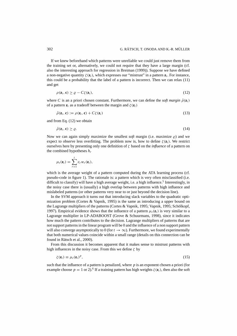
Now we can again simply maximize the smallestsoft margin (i.e. maximize%) and weexpect to observe less overfitting. The problem now is, how to defineζ(zi ). We restrictourselves here by presenting only one definition ofζ based on theinfluenceof a pattern onthe combined hypotheseshr
µt (zi ) =t∑
r=1
crwr (zi ),
which is the average weight of a pattern computed during the ATA learning process (cf.pseudo-code in figure 1). The rationale is: a pattern which is very often misclassified (i.e.difficult to classify) will have a high average weight, i.e. a high influence.5 Interestingly, inthe noisy case there is (usually) a high overlap between patterns with high influence andmislabeled patterns (or other patterns very near to or just beyond the decision line).
In the SVM approach it turns out that introducing slack variables to the quadratic opti-mization problem (Cortes & Vapnik, 1995) is the same as introducing a upper bound onthe Lagrange multipliers of the patterns (Cortes & Vapnik, 1995; Vapnik, 1995; Sch¨olkopf,1997). Empirical evidence shows that the influence of a patternµt (zi ) is very similar to aLagrange multiplier in LP-ADABOOST (Grove & Schuurmans, 1998), since it indicateshow much the pattern contributes to the decision. Lagrange multipliers of patterns that arenot support patterns in the linear program will be 0 and the influence of a non support patternwill also converge asymptotically to 0 (fort →∞). Furthermore, we found experimentallythat both numerical values coincide within a small range (details on this connection can befound in Ratsch et al., 2000).
From this discussion it becomes apparent that it makes sense to mistrust patterns withhigh influences in the noisy case. From this we defineζ by
ζ(zi ) ≡ µt (zi )p, (15)
such that the influence of a pattern is penalized, wherep is an exponent chosen a priori (forexample choosep = 1 or 2).6 If a training pattern has high weightsζ(zi ), then also the soft

SOFT MARGINS FOR ADABOOST 303
margin is increasing. If we now maximize the smallest soft margin, we do not force outliersto be classified according to their possibly wrong labels, but we allow for some errors. Ourprior for the choice (15) is to weight all patterns equally. This counterbalances the tendencyof ATAs to overweight certain patterns. So we tradeoff between margin and influence.
Note 7. If we chooseC = 0 in Eq. (12), the original ADABOOST algorithm is retrieved.If C is chosen high, then each single data point is “not taken very seriously” and we observeempirically that the number of support patterns increases. ForC→∞we (almost) retrievethe BAGGING algorithm (Breiman, 1996) (in this case, the pattern weighting will be alwaysuniform).
Of course, other functional forms ofζ are also possible (see also R¨atsch et al., 2000),for instanceζ t (zi ) = P f t (xi ), whereP is an arbitrary regularization operator. WithP it ispossible to incorporate (other) prior knowledge about the problem into ATAs like smooth-ness of the decision surface much in the spirit of Tikhonov regularizers (e.g. Tikhonov &Arsenin, 1977; Smola, Sch¨olkopf, & Muller, 1998; Rokui & Shimodaira, 1998).
Now we can reformulate the ATA optimization process in terms of soft margins. FromEq. (14) and the definition in (15) we can easily derive the new error function (cf. Eq. (2)),which aims to maximize the soft margin (we assumeφ = 1
2):
GReg(bt ) =l∑
i=1
exp
{−1
2ρ(zi , bt )
}
=l∑
i=1
exp
{−1
2|bt |[ρ(zi , ct )+ Cµt (zi )
p]
}. (16)
The weightwt+1(zi ) of a pattern is computed as the derivative of Eq. (16) with respect toρ(zi , bt ) (cf. Lemma 1)
wt+1(zi ) = 1
Zt
∂GReg(bt )
∂ρ(zi , bt )= exp{−ρ(zi , bt )/2}∑l
j=1 exp{−ρ(z j , bt )/2} , (17)
whereZt is a normalization constant such that∑l
i=1wt+1(zi ) = 1. For p = 1 we get theupdate rule for the weight of a training pattern in thet-th iteration (for details cf. R¨atsch,1998) as
wt+1(zi ) = wt (zi )
Ztexp{bt I(yi 6= ht (xi ))− Cζ t (zi )|bt |}, (18)
and for p = 2 we obtain
wt+1(zi ) = wt (zi )
Ztexp{bt I(yi 6= ht (x))− Cζ t (zi )|bt | + Cζ t−1(zi )|bt−1|}, (19)
whereZt is again a normalization constant. It is more difficult to compute the weightbt
of the t-th hypothesis analytically. However, we can getbt efficiently by a line search
304 G. RATSCH, T. ONODA AND K.-R. MULLER
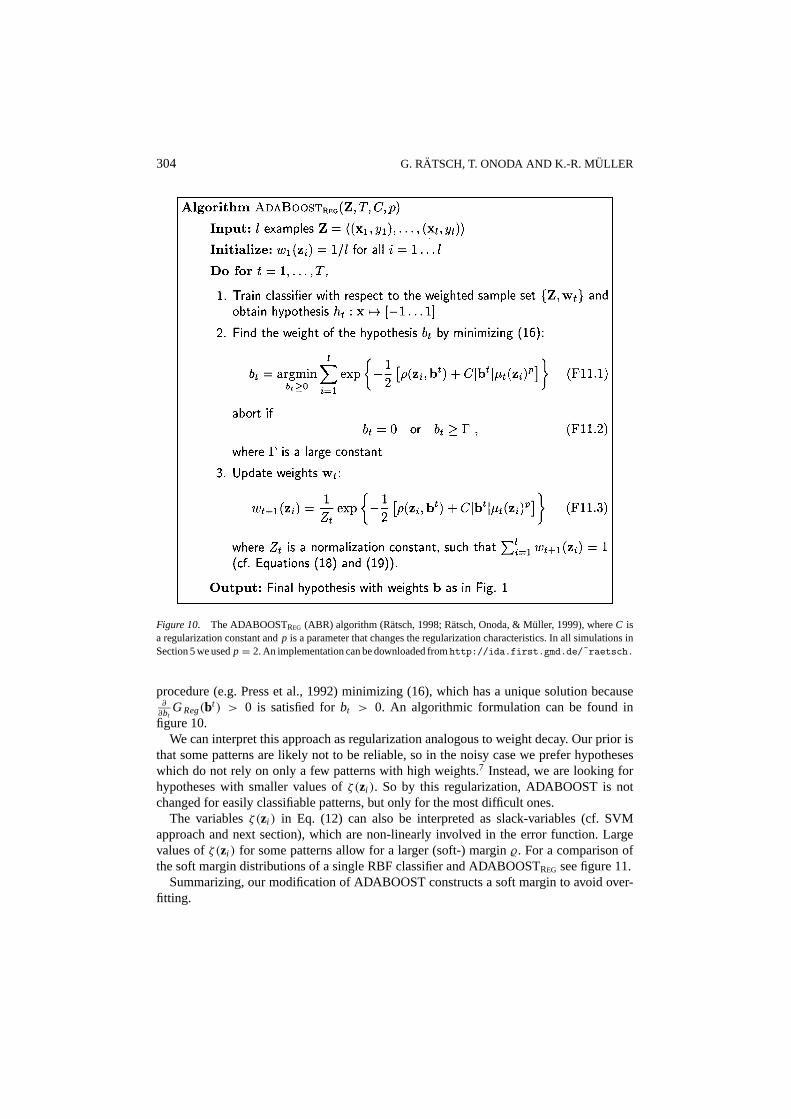
Figure 10. The ADABOOSTREG (ABR) algorithm (Ratsch, 1998; R¨atsch, Onoda, & M¨uller, 1999), whereC isa regularization constant andp is a parameter that changes the regularization characteristics. In all simulations inSection 5 we usedp = 2. An implementation can be downloaded fromhttp://ida.first.gmd.de/ ˜raetsch.
procedure (e.g. Press et al., 1992) minimizing (16), which has a unique solution because∂∂bt
GReg(bt ) > 0 is satisfied forbt > 0. An algorithmic formulation can be found infigure 10.
We can interpret this approach as regularization analogous to weight decay. Our prior isthat some patterns are likely not to be reliable, so in the noisy case we prefer hypotheseswhich do not rely on only a few patterns with high weights.7 Instead, we are looking forhypotheses with smaller values ofζ(zi ). So by this regularization, ADABOOST is notchanged for easily classifiable patterns, but only for the most difficult ones.
The variablesζ(zi ) in Eq. (12) can also be interpreted as slack-variables (cf. SVMapproach and next section), which are non-linearly involved in the error function. Largevalues ofζ(zi ) for some patterns allow for a larger (soft-) margin%. For a comparison ofthe soft margin distributions of a single RBF classifier and ADABOOSTREG see figure 11.
Summarizing, our modification of ADABOOST constructs a soft margin to avoid over-fitting.

SOFT MARGINS FOR ADABOOST 305
Figure 11. Margin distribution graphs of the RBF base hypothesis (scaled) trained with Squared Error (left) andADABOOSTREG (right) with different values ofC for the toy data set after 1000 iterations. Note that for somevalues forC the graphs of ADABOOSTREG are quite similar to the graphs of the single RBF net.
4.2. Linear programming with slack variables
Grove and Schuurmans (1998) showed how to use linear programming to maximize thesmallest margin for a given ensemble and proposed LP-ADABOOST (cf. Eq. (21)). Intheir approach, they first compute a margin (or gain) matrixM ∈ {±1}l×T for the givenhypotheses set, which is defined by
Mi,t = yi ht (xi ). (20)
M defines which hypothesis contributes a positive (or negative) part to the margin of apattern and is used to formulate the following max-min problem: find a weight vectorc ∈ RT
for hypotheses{ht }Tt=1, which maximizes the smallest margin% := mini=1,...,lρ(zi ). Thisproblem can be solved by linear programming (e.g. Mangasarian, 1965):
Maximize % subject toT∑
t=1
Mi,t ct ≥ % i = 1, . . . , l (21)
ct ≥ 0 t = 1, . . . , TT∑
t=1
ct = 1.
This LP-ADABOOST algorithm achieves a larger hard margin than the originalADABOOST algorithm, however in this form it cannot hope to generalize well on noisydata (see our discussion in Section 3). Therefore we also define a soft-margin for a patternρ ′(zi ) = ρ(zi ) + ξi , which is technically equivalent to the introduction of slack variablesξi and we arrive at the algorithm LPREG-ADABOOST (Ratsch, 1998; R¨atsch et al., 1999;Ratsch, Onoda, & M¨uller, 1998). To avoid large values of the slack variables, while solving
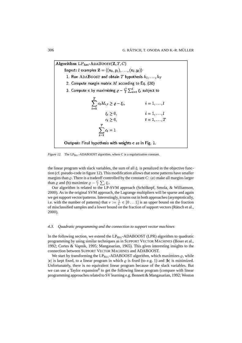
306 G. RATSCH, T. ONODA AND K.-R. MULLER
Figure 12. The LPREG-ADABOOST algorithm, whereC is a regularization constant.
the linear program with slack variables, the sum of allξi is penalized in the objective func-tion (cf. pseudo-code in figure 12). This modification allows that some patterns have smallermargins than%. There is a tradeoff controlled by the constantC: (a)make all margins largerthan% and (b) maximize% − C
l
∑i ξi .
Our algorithm is related to the LP-SVM approach (Sch¨olkopf, Smola, & Williamson,2000). As in the original SVM approach, the Lagrange multipliers will be sparse and againwe get support vector/patterns. Interestingly, it turns out in both approaches (asymptotically,i.e. with the number of patterns) thatν := 1
C ∈ [0 . . .1] is an upper bound on the fractionof misclassified samples and a lower bound on the fraction of support vectors (R¨atsch et al.,2000).
4.3. Quadratic programming and the connection to support vector machines
In the following section, we extend the LPREG-ADABOOST (LPR) algorithm to quadraticprogramming by using similar techniques as in SUPPORTVECTORMACHINES (Boser et al.,1992; Cortes & Vapnik, 1995; Mangasarian, 1965). This gives interesting insights to theconnection between SUPPORTVECTORMACHINES and ADABOOST.
We start by transforming the LPREG-ADABOOST algorithm, which maximizes%, while|c| is kept fixed, to a linear program in which% is fixed (to e.g. 1) and|b| is minimized.Unfortunately, there is no equivalent linear program because of the slack variables. Butwe can use a Taylor expansion8 to get the following linear program (compare with linearprogramming approaches related to SV learning e.g. Bennett & Mangasarian, 1992; Weston

SOFT MARGINS FOR ADABOOST 307
et al., 1997; Frieß & Harrison, 1998; Bennett, 1998):
Minimize ‖b‖1+ C∑
i
ξi subject to
T∑t=1
bt Mi,t ≥ 1− ξi , t = 1, . . . , T, (22)
bt ≥ 0, t = 1, . . . , T,
ξi ≥ 0, i = 1, . . . , l .
Essentially, this is the same algorithm as in figure 12: for a different value ofC problem,(22) is equivalent to the one in figure 12 (cf. Smola, 1998 and Lemma 3 in R¨atsch et al.,2000). Instead of using the1-norm in the optimization objective of (22), we can also usethe`p-norm. Clearly, eachp will imply its own soft margin characteristics. Usingp = 2leads to an algorithm similar to the SVM (cf. figure 14).
The optimization objective of a SVM is to find a functionhw which minimizes a functionalof the form (Vapnik, 1995)
E = ‖w‖2+ Cl∑
i=1
ξi , (23)
subject to the constraints
yi h(xi ) ≥ 1− ξi and ξi ≥ 0, for i = 1, . . . , l .
Here, the variablesξi are the slack-variables responsible for obtaining a soft margin. Thenorm of the parameter vectorw defines a system of nested subsets in the combined hypoth-esis space and can be regarded as a measure of the complexity (as also the size of the margin
Figure 13. Margin distribution graphs of LPREG-ADABOOST (left) and QPREG-ADABOOST (right) for differentvalues ofC for the toy data set after 1000 iterations. LPREG-ADABOOST sometimes generates margins on thetraining set, which are either 1 or−1 (step in the distribution).
308 G. RATSCH, T. ONODA AND K.-R. MULLER
of hypothesishw) (Vapnik, 1995). With functional (23), we get a tradeoff (controlled byC)between the complexity of the hypothesis (‖w‖2) and the degree how much the classificationmay differ from the labels of the training patterns (
∑i ξi ).
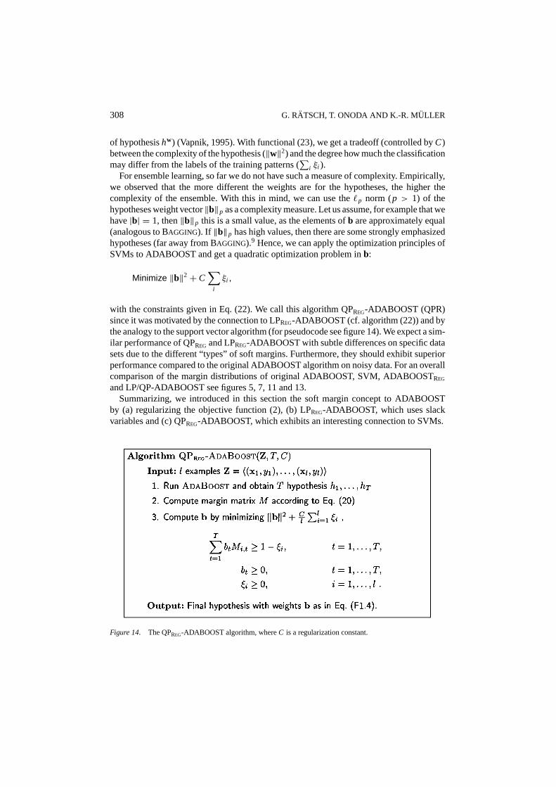
For ensemble learning, so far we do not have such a measure of complexity. Empirically,we observed that the more different the weights are for the hypotheses, the higher thecomplexity of the ensemble. With this in mind, we can use the`p norm (p > 1) of thehypotheses weight vector‖b‖p as a complexity measure. Let us assume, for example that wehave|b| = 1, then‖b‖p this is a small value, as the elements ofb are approximately equal(analogous to BAGGING). If ‖b‖p has high values, then there are some strongly emphasizedhypotheses (far away from BAGGING).9 Hence, we can apply the optimization principles ofSVMs to ADABOOST and get a quadratic optimization problem inb:
Minimize ‖b‖2+ C∑
i
ξi ,
with the constraints given in Eq. (22). We call this algorithm QPREG-ADABOOST (QPR)since it was motivated by the connection to LPREG-ADABOOST (cf. algorithm (22)) and bythe analogy to the support vector algorithm (for pseudocode see figure 14). We expect a sim-ilar performance of QPREG and LPREG-ADABOOST with subtle differences on specific datasets due to the different “types” of soft margins. Furthermore, they should exhibit superiorperformance compared to the original ADABOOST algorithm on noisy data. For an overallcomparison of the margin distributions of original ADABOOST, SVM, ADABOOSTREG
and LP/QP-ADABOOST see figures 5, 7, 11 and 13.Summarizing, we introduced in this section the soft margin concept to ADABOOST
by (a) regularizing the objective function (2), (b) LPREG-ADABOOST, which uses slackvariables and (c) QPREG-ADABOOST, which exhibits an interesting connection to SVMs.
Figure 14. The QPREG-ADABOOST algorithm, whereC is a regularization constant.

SOFT MARGINS FOR ADABOOST 309
5. Experiments
In order to evaluate the performance of our new algorithms, we perform large scale simula-tions and compare the single RBF classifier, the original ADABOOST algorithm,ADABOOSTREG, L/QPREG-ADABOOST and a SUPPORTVECTOR MACHINE (with RBFkernel).
5.1. Experimental setup
For this, we use 13 artificial and real world data sets from the UCI, DELVE and STAT-LOG benchmark repositories10: banana (toy data set used in the previous sections),breastcancer,11 diabetes, german, heart, image segment, ringnorm, flare solar, splice, new-thyroid, titanic, twonorm, waveform. Some of the problems are originally not binary classi-fication problems, hence a random partition into two classes is used.12 At first we generate100 partitions into training and test set (mostly≈ 60% : 40%). On each partition we traina classifier and then compute its test set error.
In all experiments, we combine 200 hypotheses. Clearly, this number of hypotheses issomewhat arbitrary and may not be optimal. However we checked that original ADABOOSTwith early stopping is most of the time worse than any of the proposed soft margin algorithms(cf. an earlier study R¨atsch, 1998). However, we use a fixed number of iterations for allalgorithms, therefore this comparison should be fair.
As base hypotheses we use RBF nets with adaptive centers as described in Appendix D.On each of the 13 data sets we employ cross validation to find the best base hypothesismodel, which is then used in the ensemble learning algorithms. For selecting the best RBFmodel we optimize the number of centers (parameterK , cf. figure 15) and the number ofiteration steps for adapting the RBF centers and widths (parameterO). The parameterλwas fixed to 10−6.
The parameterC of the regularized versions of ADABOOST and the parameters (C, σ )of the SVM (C is the regularization constant andσ is the width of the RBF-kernel be-ing used) are optimized on the first five realizations of each data set. On each of theserealizations, a 5-fold-cross validation procedure gives a good model.13 Finally, the modelparameters are computed as the median of the five estimations and used throughout thetraining on all 100 realization of that data set. This way of estimating the parameters iscomputationally highly expensive, but it will make our comparison more robust and theresults more reliable.
Note, to perform the simulations in this setup we had to train more than 3×10⁶ adaptiveRBF nets and to solve more than 105 linear or quadratic programming problems—a task thatwould have taken altogether 2 years of computing time on a single Ultra-SPARC machine,if we had not distributed it over 30 computers.
5.2. Experimental results
In Table 1 the average generalization performance (with standard deviation) over the 100partitions of the data sets is given. The second last line in Table 1 showing ‘Mean%’, is

310 G. RATSCH, T. ONODA AND K.-R. MULLER
Figure 15. Pseudo-code description of the RBF net algorithm, which is used as base learning algorithm in thesimulations with ADABOOST.
computed as follows: For each data set the average error rates of all classifier types aredivided by the minimum error rate for this data set and 1 is subtracted. These resultingnumbers are averaged over the 13 data sets and the variance is computed. The last line givesthe Laplacian probability (and variance) over 13 data sets whether a particular methodwins on a particular realization of a data set, i.e. has the lowest generalization error. Ourexperiments on noisy data (cf. Table 1) show that:
– The results of ADABOOST are in almost all cases worse than the single classifier. Thisis clearly due to the overfitting of ADABOOST. If early stopping is used then the effectis less drastic but still clearly observable (R¨atsch, 1998).
– The averaged results for ADABOOSTREG are a bit better (Mean% and Winner%) thanthe results of the SVM, which is known to be an excellent classifier. In five (out ofseven) cases ADABOOSTREG is significant better than the SVM. Moreover, the single

SOFT MARGINS FOR ADABOOST 311
Table 1. Comparison among the six methods: Single RBF classifier, ADABOOST (AB), ADABOOSTREG (ABR;p = 2), L/QPREG-ADABOOST (L/QPR-AB) and a SUPPORTVECTOR MACHINE: Estimation of generalizationerror in % on 13 data sets (best method in bold face, second emphasized). The columns S1 and S2 show the resultsof a significance test (95%-t-test) between AB/ABR and ABR/SVM, respectively. ADABOOSTREG gives the bestoverall performance.
RBF AB S1 ABR LPR-AB QPR-AB S2 SVM
Banana 10.8± 0.6 12.3± 0.7 + 10.9± 0.4 10.7± 0.4 10.9± 0.5 + 11.5± 0.7
B. Cancer 27.6± 4.7 30.4± 4.7 + 26.5± 4.5 26.8± 6.1 25.9± 4.6 26.0± 4.7
Diabetes 24.3± 1.9 26.5± 2.3 + 23.8± 1.8 24.1± 1.9 25.4± 2.2 + 23.5± 1.7
German 24.7± 2.4 27.5± 2.5 + 24.3± 2.1 24.8± 2.2 25.3± 2.1 − 23.6± 2.1
Heart 17.6± 3.3 20.3± 3.4 + 16.5± 3.5 17.5± 3.5 17.2± 3.4 16.0± 3.3
Image 3.3± 0.6 2.7± 0.7 2.7± 0.6 2.8± 0.6 2.7± 0.6 3.0± 0.6
Ringnorm 1.7± 0.2 1.9± 0.3 + 1.6± 0.1 2.2± 0.5 1.9± 0.2 + 1.7± 0.1
F. Solar 34.4± 2.0 35.7± 1.8 + 34.2± 2.2 34.7± 2.0 36.2± 1.8 − 32.4± 1.8
Splice 10.0± 1.0 10.1± 0.5 + 9.5± 0.7 10.2± 1.6 10.1± 0.5 + 10.9± 0.7
Thyroid 4.5± 2.1 4.4± 2.2 − 4.6± 2.2 4.6± 2.2 4.4± 2.2 4.8± 2.2
Titanic 23.3± 1.3 22.6± 1.2 22.6± 1.2 24.0± 4.4 22.7± 1.1 22.4± 1.0
Twonorm 2.9± 0.3 3.0± 0.3 + 2.7± 0.2 3.2± 0.4 3.0± 0.3 + 3.0± 0.2
Waveform 10.7± 1.1 10.8± 0.6 + 9.8± 0.8 10.5± 1.0 10.1± 0.5 9.9± 0.4
Mean% 6.6± 5.8 11.9± 7.9 1.7± 1.9 8.9± 10.8 5.8± 5.5 4.6± 5.4
Winner% 14.8± 8.5 7.2± 7.8 26.0± 12.4 14.4± 8.6 13.2± 7.6 23.5± 18.0
RBF classifier wins less often than the SVM (for a comparison in the regression case cf.Muller et al., 1998).
– L/QPREG-ADABOOST improves the results of ADABOOST. This is due to the use ofa soft margin. But the results are not as good as the results of ADABOOSTREG and theSVM. One reason is that the hypotheses generated by ADABOOST (aimed to constructa hard margin) may not provide the appropriate basis to subsequently generate a goodsoft margin with linear and quadratic programming approaches.
– We can observe that quadratic programming gives slightly better results than linearprogramming. This may be due to the fact that the hypotheses coefficients generated byLPREG-ADABOOST are more sparse (smaller ensemble) and larger ensembles may havea better generalization ability (Breiman, 1998). Furthermore, with QP-ADABOOST weprefer ensembles which have approximately equally weighted hypotheses. As stated inSection 4.3, this implies a lower complexity of the combined hypothesis, which can leadto a better generalization performance.
– The results of ADABOOSTREG are in ten (out of 13) cases significantly better than theresults of ADABOOST. Also, in ten cases ADABOOSTREG performs better than thesingle RBF classifier.
Summarizing, ADABOOSTREG wins most often and shows the best average performance.In most of the cases it performs significantly better than ADABOOST and it performs

312 G. RATSCH, T. ONODA AND K.-R. MULLER
slightly better than SUPPORTVECTORMACHINES. This demonstrates the noise robustnessof the proposed algorithm.
The slightly inferior performance of SVM compared to ADABOOSTREG may be ex-plained with the fixedσ of the RBF-kernel for SVM. By fixingσ we look at the data onlyatone scale, i.e. we are losing possible multiscale information that could be inherent of thedata. Further causes could be the coarse model selection, and the error function of the SValgorithm, which is not adapted to the noise model in the data (see Smola et al., 1998).
So, the original ADABOOST algorithm is useful forlow noise cases, where the classesare easily separable (as shown for OCR cf. Schwenk & Bengio, 1997; LeCun et al., 1995).L/QPREG-ADABOOST can improve the ensemble structure through introducing a soft mar-gin and the same hypotheses (just with another weighting) can result in a much better gen-eralization performance. The hypotheses, which are used by L/QPREG-ADABOOST maybe sub-optimal, because they are not part of the L/QP optimization process that aims fora soft margin. ADABOOSTREG does not have this problem: the hypotheses are generatedsuch that they are appropriate to form the desired soft-margin. ADABOOSTREG extends theapplicability of Boosting/Arcing methods to non-separable cases and should be preferablyapplied if the data is noisy.
6. Conclusion
We have shown that ADABOOST performs a constrained gradient descent in an error func-tion that optimizes the margin (cf. Eq. (2)). Asymptotically, all emphasis is concentrated onthe difficult patterns with small margins, easy patterns effectively do not contribute to theerror measure and are neglected in the training process (very much similar to support vec-tors). It was shown theoretically and experimentally that the cumulative margin distributionof the training patterns converges asymptotically to a step. Therefore, original ADABOOSTachieves ahard marginclassification asymptotically. The asymptotic margin distributionof ADABOOST and SVM (for the separable case) are very similar. Hence, the patternslying in the step part (support patterns) of the margin distribution show a large overlap tothe support vectors found by a SVM.
We discussed in detail that ATAs and hard margin classifiers are in general noise sensitiveand prone to overfit. We introduced three regularization-based ADABOOST algorithms toalleviate this overfitting problem: (1) direct incorporation of the regularization term intothe error function (ADABOOSTREG), use of (2) linear and (3) quadratic programming withslack variables to improve existing ensembles. The essence of our proposed algorithms isto achieve a soft margin (through regularization term and slack variables) in contrast to thehard margin classification used before. The soft-margin approach allows to control howmuch we trust the data, so we are permitted to ignore noisy patterns (e.g. outliers) whichwould otherwise spoile our classification. This generalization is very much in the spirit ofSUPPORTVECTOR MACHINES that also tradeoff the maximization of the margin and theminimization of the classification errors by introducing slack variables. Note that we justgave one definition for the soft margin in ADABOOSTREG other extensions that e.g. useregularization operators (e.g. Smola et al., 1998; Rokui & Shimodaira, 1998; Bishop, 1995)or that have other functional forms (cf. R¨atsch et al., 2000) are also possible.

SOFT MARGINS FOR ADABOOST 313
In our experiments on noisy data the proposed regularized versions of ADABOOST:ADABOOSTREG and L/QPREG-ADABOOST show a more robust behavior than the originalADABOOST algorithm. Furthermore, ADABOOSTREG exhibits a better overall general-ization performance than all other analyzed algorithms including the SUPPORTVECTOR
MACHINES. We conjecture that this result is mostly due to the fact that SUPPORTVECTOR
MACHINEScan only use oneσ , i.e. only one–fixed–kernel, and therefore loses multi-scalinginformation. ADABOOST does not have this limitation, since we use RBF nets with adap-tive kernel widths as base hypotheses.
Our future work will concentrate on a continuing improvement of ADABOOST-typealgorithms for noisy real world applications. Also, a further analysis of the relation betweenADABOOST (in particular QPREG-ADABOOST) and SUPPORTVECTORMACHINES fromthe margin point of view seems promising, with particular focus on the question of what goodmargin distributions should look like. Moreover, it is interesting to see how the techniquesestablished in this work can be applied to ADABOOST in a regression scenario (cf. Bertoni,Campadelli, & Parodi, 1997; Friedman, 1999; R¨atsch et al., 2000).
Appendix
A. Proof of Lemma 1
Proof: We defineπt (zi ) := ∏tr=1 exp(−br I(hr (zi ) = yi )) and from definition ofG and
d we get
∂G∂ρ(zi ,bt )∑l
j=1∂G
∂ρ(z j ,bt )
= exp(− 1
2ρ(zi , bt ))∑l
j=1 exp(− 1
2ρ(zi , bt ))
= πt (zi )∑lj=1πt (x j )
= πt (zi )
Zt
,
where Zt := ∑li=1πt (zi ). By definition,πt (zi ) = πt−1(zi ) exp(−bt I(ht (zi ) = yi )) and
π1(zi ) = 1/ l . Thus, we get
wt+1(zi ) = πt (zi )
Zt
= πt−1(zi ) exp(−bt I(ht (zi ) = yi ))
Zt
= wt−1(zi )Zt−1 exp(−bt I(ht (zi ) = yi ))
Zt
= wt−1(zi ) exp(−bt I(ht (zi ) = yi ))
Zt,
whereZt = Zt Zt−1 (cf. step 4 in figure 1). 2

314 G. RATSCH, T. ONODA AND K.-R. MULLER
B. Proof of Theorem 3
The proof follows the one of Theorem 5 in (Schapire et al., 1997). Theorem 3 is a general-ization forφ 6= 1
2.
Proof: If y f (x) ≤ θ , then we have
yT∑
t=1
btht (x) ≤ θT∑
t=1
bt ,
and also
exp
{− y
2
T∑t=1
bt ht (x)+ θ2
T∑t=1
bt
}≥ 1.
Thus,
P(x,y)∼Z [y f (x) ≤ θ ] ≤ 1
l
l∑i=1
exp
{− yi
2
T∑t=1
btht (xi )+ θ2
T∑t=1
bt
}
= exp(θ2
∑Tt=1 bt
)l
l∑i=1
exp
{− yi
2
T∑t=1
bt ht (xi )
},
where
l∑i=1
exp
{− yi
2
T∑t=1
btht (xi )
}
=l∑
i=1
exp
{− yi
2
T−1∑t=1
btht (xi )
}exp
{− yi
2bT hT (xi )
}
=∑
i :hT (xi )=yi
exp
{− yi
2
T−1∑t=1
btht (xi )
}e−bT/2
+∑
i :hT (xi )6=yi
exp
{− yi
2
T−1∑t=1
btht (xi )
}ebT/2
=(
l∑i=1
exp
{− yi
2
T−1∑t=1
bt ht (xi )
})((1− εT )e
−bT/2+ εTebT/2),
because
εT = 1∑lj=1w
Tj
∑i :hT (xi )6=yi
wTi .

SOFT MARGINS FOR ADABOOST 315
With∑l
i=1 exp(0) = l (for t = 1), we get recursively
P(x,y)∼Z [y f (x) ≤ θ ] ≤ exp
(θ
2
T∑t=1
bt
)T∏
t=1
((1− εt )e−bt/2+ εt e
bt/2).
Plugging in the definition forbt we get
P(x,y)∼Z [y f (x) ≤ θ ] ≤(
T∏t=1
1− εt
εt
T∏t=1
φ
1− φ
)θ/2
×(√
φ
1− φ +√
1− φφ
)T T∏t=1
√(1− εt ) εt
=((
φ
1− φ) 1+φ
2
+(
1− φφ
) 1−φ2
)T T∏t=1
√(1− εt )1+θ ε1−θ
t
= (ϕ 1+θ2 + ϕ− 1−θ
2)T
T∏t=1
√ε1−θ
t (1− εt )1+θ .
2
C. Proof of Lemma 5
Proof: We have to show that limt→∞ εt = 0, where
εt :=∣∣∣mini :yi=1
ρ(zi , ct )− minj :yj=−1
ρ(z j , ct )
∣∣∣.The setSt
c is the set of support patterns at iterationt :
Stc =
{j ∈ {1, . . . , l } : ρ(z j , ct ) = min
i :yi=cρ(zi , ct )
},
which clearly contains at least one element. Note thatS∞1 ∪S∞−1 is the set of support patterns,which we will get asymptotically.
Suppose we haveεt > 1/2 > 0 ands ∈ {±1} is the class with the smallest margin.With (4), q ∈ St
s andQ := exp(− 12ρ(zq, ct )) we get
∑i :yi=s
wt (zi ) ≥ Q|bt |
Q|bt | +∑i :yi 6=s exp(− 1
2ρ(zi , ct ))|bt |
>Q|b
t |
Q|bt | + (l − 1)Q|bt |e−|bt |1/4

316 G. RATSCH, T. ONODA AND K.-R. MULLER
With |bt |> tγ from assumption (8) we get∑
i :yi = swt (zi )≥ δ, for t > t1 := log(l−1)−log(1/δ−1)γ1/4 .
Hence, with assumption (9) we get: Ift ≥ t1, then all patternszi of classs will be clas-sified correctly and patterns of classr = −s will be misclassified. Therefore, we obtainρ(zi , ct+1) = |bt |ρ(zi ,ct )+bt+1
|bt+1| , for i ∈ {k : yk = s} (especially fori ∈ Sts). The patterns of
classr will be misclassified and we haveρ(z j , ct+1) = |bt |ρ(z j ,ct )−bt+1
|bt+1| , for j ∈ {k : yk = r }.It follows
εt+1 =∣∣∣∣mini :yi=s
|bt |ρ(zi , ct )− bt+1
|bt+1| − minj :yj=r
|bt |ρ(z j , ct )+ bt+1
|bt+1|∣∣∣∣
=∣∣∣∣εt |bt | − 2bt+1
|bt+1|∣∣∣∣
As long asεt > 1/2, all patterns of classr will be misclassified and patterns of classswill be classified correctly. If it becomes(εt |bt | − 2bt+1)/|bt+1| < −1/2, then the samereasoning can be done interchanging the role ofs andr . If furthermoret > t2 := 40
γ1, then
εt |bt | − 2bt+1 > 0 and we haveεt+1 < εt − ωt , whereωt is decreasing not too fast (i.e. itcan be bounded byO(1/t)). Hence, we will reach the caseεt < 1/2 and get: Ift is largeenough(t > t3 := 20(2−1)
1γ), then
−1 <εt |bt | − 2bt+1
|bt+1| < 1,
i.e. adding a new hypothesis will not lead toεt+1 ≥ 1.Therefore, after a finite numbert of subsequent steps, we have we will reachεt < 1.
Furthermore, the discussion above shows that, ift is large enough, it is not possible to leavethe1area around 0. Hence, for each1 > 0, we can provide an indexT = max(t1, t2, t3)+ t(wheret1, . . . , t3 are the lower bounds ont used above), such thatεt < 1 for all t > T .This implies the desired result. 2
D. RBF nets with adaptive centers
The RBF nets used in the experiments are an extension of the method of Moody and Darken(1989), since centers and variances are also adapted (see also Bishop, 1995; M¨uller et al.,1998). The output of the network is computed as a linear superposition ofK basis functions
f (x) =K∑
k=1
wkgk(x), (24)
wherewk, k = 1, . . . , K , denotes the weights of the output layer. The Gaussian basisfunctionsgk are defined as
gk(x) = exp
(−‖x− µk‖2
2σ 2k
), (25)

SOFT MARGINS FOR ADABOOST 317
whereµk andσ 2k denote means and variances, respectively. In a first step, the meansµk
are initialized with K-means clustering and the variancesσk are determined as the distancebetweenµk and the closestµi (i 6= k, i ∈ {1, . . . , K }). Then in the following steps weperform a gradient descent in the regularized error function (weight decay)
E = 1
2
l∑i=1
(yi − f (xi ))2+ λ
2l
K∑k=1
w2k. (26)
Taking the derivative of Eq. (26) with respect to RBF meansµk and variancesσk we obtain
∂E
∂µk=
l∑i=1
( f (xi )− yi )∂
∂µkf (xi ), (27)
with ∂∂µk
f (xi ) = wkxi−µk
σ 2k
gk(xi ) and
∂E
∂σk=
l∑i=1
( f (xi )− yi )∂
∂σkf (xi ), (28)
with ∂∂σk
f (xi ) = wk‖µk−xi ‖2
σ 3k
gk(xi ). These two derivatives are employed in the minimizationof Eq. (26) by a conjugate gradient descent with line search, where we always compute theoptimal output weights in every evaluation of the error function during the line search. Theoptimal output weightsw = [w1, . . . , wK ]> in matrix notation can be computed in closedform by
w =(
GT G+ 2λ
lI)−1
GTy, whereGik = gk(xi ) (29)
andy = [y1, . . . , yl ]> denotes the output vector, andI an identity matrix. Forλ = 0, thiscorresponds to the calculation of a pseudo-inverse of G.
So, we simultaneously adjust the output weights and the RBF centers and variances (seefigure 15 for pseudo-code of this algorithm). In this way, the network fine-tunes itself tothe data after the initial clustering step, yet, of course, overfitting has to be avoided bycareful tuning of the regularization parameter, the number of centersK and the number ofiterations (cf. Bishop, 1995). In our experiments we always usedλ = 10−6 and up to tenCG iterations.
Acknowledgments
We thank for valuable discussions with B. Sch¨olkopf, A. Smola, T. Frieß, D. Schuurmansand B. Williamson. Partial funding from EC STORM project number 25387 is gratefullyacknowledged. Furthermore, we acknowledge the referees for valuable comments.

318 G. RATSCH, T. ONODA AND K.-R. MULLER
Notes
1. An ensemble is a collection of neural networks or other types of classifiers (hypotheses) that are trained forthe same task.
2. In Friedman et al. (1998) it was mentioned that sometimes the randomized version shows a better performance,than the version with weighted minimization. In connection with the discussion in Section 3 this becomesclearer, because the randomized version will show an overfitting effect (possibly much) later and overfittingmay be not observed, whereas it was observed using the more efficient weighted minimization.
3. In our experiments we have often observed values for|b| that are larger than 100 after only 200 iterations.4. A detailed description of the generation of the toy data used in the asymptotical simulations can be found in
the Internethttp://ida.first.gmd.de/ ˜ raetsch/data/banana.html.5. The definition of the influence clearly depends on the base hypothesis spaceH. If the hypothesis space
changes, other patterns may be more difficult to classify.6. Note that forp = 1 there is a connection to the leave-one-out-SVM approach of Weston (1999).7. Interestingly, the (soft) SVM generates many more support vectors in the high noise case than in the low noise
case (Vapnik, 1995).8. From the algorithm in figure 12, it is straight forward to get the following linear program, which is equivalent
for any fixedS> 0:
Minimize%+
S+ C
S
∑i
ξ+i subject to ST∑
t=1
ct Mi,t ≥ %+ − ξ+i ,
where%+ := S%, ξ+i := Sξi , bt ≥ 0, ξ+i ≥ 0,∑
t
bt = S.
In this problem we can set%+ to 1 and try to optimizeS. To retrieve a linear program, we use the Taylorexpansion around 1:1S = S+O((S−1)2) and
∑i ξ+i /S=
∑i ξ+i +O(S−1). ForS= |b|we get algorithm
(22).9. For p = 2, ‖b‖2 corresponds to the Renyi entropy of the hypothesis vector and we are effectively trying to
minimize this entropy while separating the data.10. These data sets including a short description, the splits into the 100 realizations and the simulation results are
available athttp://ida.first.gmd.de/ ˜ raetsch/data/benchmarks.htm.11. The breast cancer domain was obtained from the University Medical Center, Inst. of Oncology, Ljubljana,
Yugoslavia. Thanks go to M. Zwitter and M. Soklic for providing the data.12. A random partition generates a mappingm of n to two classes. For this a random±1 vectorm of lengthn is
generated. The positive classes (and the negative respectively) are then concatenated.13. The parameters selected by the cross validation are only near-optimal. Only 15–25 values for each parameter
are tested in two stages: first a global search (i.e. over a wide range of the parameter space) was done to finda good guess of the parameter, which becomes more precise in the second stage.
References
Bennett, K. (1998). Combining support vector and mathematical programming methods for induction. In B.Scholkopf, C. Burges, & A. Smola (Eds.),Advances in kernel methods—SV learning. Cambridge, MA: MITPress.
Bennett, K. & Mangasarian, O. (1992). Robust linear programming discrimination of two linearly inseparablesets.Optimization Methods and Software, 1, 23–34.
Bertoni, A., Campadelli, P., & Parodi, M. (1997). A boosting algorithm for regression. In W. Gerstner, A. Germond,M. Hasler, & J.-D. Nicoud (Eds.),LNCS, Vol. V: Proceedings ICANN’97: Int. Conf. on Artificial Neural Networks(pp. 343–348). Berlin: Springer.
Bishop, C. (1995).Neural Networks for Pattern Recognition. Oxford: Clarendon Press.

SOFT MARGINS FOR ADABOOST 319
Boser, B., Guyon, I., & Vapnik, V. (1992). A training algorithm for optimal margin classifiers. In D. Haussler(Ed.),Proceedings COLT’92: Conference on Computational Learning Theory(pp. 144–152). New York, NY:ACM Press.
Breiman, L. (1996). Bagging predictors.Mechine Learning, 26(2), 123–140.Breiman, L. (1997a). Arcing the edge. Technical Report 486, Statistics Department, University of California.Breiman, L. (1997b). Prediction games and arcing algorithms. Technical Report 504, Statistics Department,
University of California.Breiman, L. (1998). Arcing classifiers.The Annals of Statistics, 26(3), 801–849.Breiman, L. (1999). Using adaptive bagging to debias regressions. Technical Report 547, Statistics Department,
University of California.Cortes, C. & Vapnik, V. (1995). Support vector networks.Machine Learning, 20, 273–297.Frean, M. & Downs, T. (1998). A simple cost function for boosting. Technical Report, Department of Computer
Science and Electrical Engineering, University of Queensland.Freund, Y. & Schapire, R. (1994). A decision-theoretic generalization of on-line learning and an applica-
tion to boosting. InProceedings EuroCOLT’94: European Conference on Computational Learning Theory.LNCS.
Freund, Y. & Schapire, R. (1996). Game theory, on-line prediction and boosting. InProceedings COLT’86: Conf.on Comput. Learning Theory(pp. 325–332). New York, NY: ACM Press.
Friedman, J. (1999). Greedy function approximation. Technical Report, Department of Statistics, StanfordUniversity.
Friedman, J., Hastie, T., & Tibshirani, R. (1998). Additive logistic regression: A statistical view of boosting.Technical Report, Department of Statistics, Sequoia Hall, Stanford University.
Frieß, T. & Harrison, R. (1998). Perceptrons in kernel feature space. Research Report RR-720, Department ofAutomatic Control and Systems Engineering, University of Sheffield, Sheffield, UK.
Grove, A. & Schuurmans, D. (1998). Boosting in the limit: Maximizing the margin of learned ensembles. InProceedings of the Fifteenth National Conference on Artifical Intelligence.
Kirkpatrick, S. (1984). Optimization by simulated annealing: Quantitative studies.J. Statistical Physics, 34, 975–986.
LeCun, Y., Jackel, L., Bottou, L., Cortes, C., Denker, J., Drucker, H., Guyon, I., M¨uller, U., Sackinger, E., Simard,P., & Vapnik, V. (1995). Learning algorithms for classification: A comparism on handwritten digit recognition.Neural Networks, 261–276.
Mangasarian, O. (1965). Linear and nonlinear separation of patterns by linear programming.Operations Research,13, 444–452.
Mason, L., Bartlett, P. L., & Baxter, J. (2000a). Improved generalization through explicit optimization of margins.Machine Learning 38(3), 243–255.
Mason, L., Baxter, J., Bartlett, P. L., & Frean, M. (2000b). Functional gradient techniques for combining hypotheses.In A. J. Smola, P. Bartlett, B. Sch¨olkopf, & C. Schuurmans (Eds.),Advances in Large Margin Classifiers.Cambridge, MA: MIT Press.
Moody, J. & Darken, C. (1989). Fast learning in networks of locally-tuned processing units.Neural Computation,1(2), 281–294.
Muller, K.-R., Smola, A., R¨atsch, G., Sch¨olkopf, B., Kohlmorgen, J., & Vapnik, V. (1998). Using support vectormachines for time series prediction. In B. Sch¨olkopf, C. Burges, & A. Smola (Eds.),Advances in KernelMethods—Support Vector Learning. Cambridge, MA: MIT Press.
Onoda, T., R¨atsch, G., & Muller, K.-R. (1998). An asymptotic analysis of ADABOOST in the binary classificationcase. In L. Niklasson, M. Bod´en, & T. Ziemke (Eds.),Proceedings ICANN’98: Int. Conf. on Artificial NeuralNetworks(pp. 195–200).
Onoda, T., R¨atsch, G., & Muller, K.-R. (2000). An asymptotical analysis and improvement of ADABOOST in thebinary classification case.Journal of Japanese Society for AI, 15(2), 287–296 (in Japanese).
Press, W., Flannery, B., Teukolsky, S., & Vetterling, W. (1992).Numerical Recipes in C(2nd ed.). Cambridge:Cambridge University Press.
Quinlan, J. (1992).C4.5: Programs for Machine Learning. Los Altos, CA: Morgan Kaufmann.Quinlan, J. (1996). Boosting first-order learning. In S. Arikawa & A. Sharma (Eds.),LNAI, Vol. 1160: Proceedings
of the 7th International Workshop on Algorithmic Learning Theory(pp. 143–155). Berlin: Springer.

320 G. RATSCH, T. ONODA AND K.-R. MULLER
Ratsch, G. (1998). Ensemble learning methods for classification. Master’s Thesis, Department of Computer Sci-ence, University of Potsdam, Germany (in German).
Ratsch, G., Onoda, T., & M¨uller, K.-R. (1998). Soft margins for ADABOOST. Technical Report NC-TR-1998-021,Department of Computer Science, Royal Holloway, University of London, Egham, UK.
Ratsch, G., Onoda, T., & M¨uller, K.-R. (1999). Regularizing ADABOOST. In M. Kearns, S. Solla, & D. Cohn(Eds.),Advances in Neural Information Processing Systems 11(pp. 564–570). Cambridge, MA: MIT Press.
Ratsch, G., Sch¨olkopf, B., Smola, A., Mika, S., Onoda, T., & M¨uller, K.-R. (2000). Robust ensemble learning. In A.Smola, P. Bartlett, B. Sch¨olkopf, & D. Schuurmans (Eds.),Advances in Large Margin Classifiers(pp. 207–219).Cambridge, MA: MIT Press.
Ratsch, G., Warmuth, M., Mika, S., Onoda, T., Lemm, S., & M¨uller, K.-R. (2000). Barrier boosting. InProceedingsCOLT’00: Conference on Computational Learning Theory(pp. 170–179). Los Altos, CA: Morgan Kaufmann.
Rokui, J. & Shimodaira, H. (1998). Improving the generalization performance of the minimum classification errorlearning and its application to neural networks. InProc. of the Int. Conf. on Neural Information Processing(ICONIP) (pp. 63–66). Japan, Kitakyushu.
Schapire, R. (1999). Theoretical views of boosting. InProceedings EuroCOLT’99: European Conference onComputational Learning Theory.
Schapire, R., Freund, Y., Bartlett, P., & Lee, W. (1997). Boosting the margin: A new explanation for the effectivenessof voting methods. InProceedings ICML’97: International Conference on Machine Learning(pp. 322–330).Los Altos, CA: Morgan Kaufmann.
Schapire, R. & Singer, Y. (1998). Improved boosting algorithms using confidence-rated predictions. InProceedingsCOLT’98: Conference on Computational Learning Theory(pp. 80–91).
Scholkopf, B. (1997).Support Vector Learning. R. Oldenbourg Verlag, Berlin.Scholkopf, B., Smola, A., & Williamson, R. (2000). New support vector algorithms.Neural Computation. also
NeuroCOLT TR–31–89, 12:1083–1121.Schwenk, H. & Bengio, Y. (1997). AdaBoosting neural networks. In W. Gerstner, A. Germond, M. Hasler, &
J.-D. Nicoud (Eds.),Proceedings ICANN’97: Int. Conf. on Artificial Neural Networks, Vol. 1327 of LNCS(pp. 967–972). Berlin: Springer.
Smola, A. J. (1998). Learning with kernels. Ph.D. Thesis, Technische Universit¨at Berlin.Smola, A., Sch¨olkopf, B., & Muller, K.-R. (1998). The connection between regularization operators and support
vector kernels.Neural Networks, 11, 637–649.Tikhonov, A. & Arsenin, V. (1977).Solutions of Ill-Posed Problems. Washington, D.C.: W.H. Winston.Vapnik, V. (1995).The Nature of Statistical Learning Theory. Berlin: Springer.Weston, J. (1999). LOO-support vector machines. InProceedings of IJCNN’99.Weston, J., Gammerman, A., Stitson, M. O., Vapnik, V., Vovk, V., & Watkins, C. (1997). Density estimation using
SV machines. Technical Report CSD-TR-97-23, Royal Holloway, University of London, Egham, UK.
Received August 14, 1998Revised June 14, 1999Accepted October 27, 1999Final manuscript September 18, 2000