Sociolinguistic data calls for mixed models 1 · Sociolinguistic data calls for mixed models 2!...

Sociolinguistic data calls for mixed models

1

Progress in regression: why sociolinguistic data calls for mixed-‐effects models

Daniel Ezra Johnson

4317 Spruce Street #202

Philadelphia, PA 19104

(347) 400-‐5214

Short title: Sociolinguistic data calls for mixed models


2

Progress in regression: why sociolinguistic data calls for mixed-‐effects models

Sociolinguistic data should not, in general, be analyzed with ordinary fixed-‐effects

regression models, such as VARBRUL and GoldVarb use. Tokens of linguistic

variables observed in natural speech are rarely independent. They can usually be

grouped, whether in a balanced or an unbalanced way, according to the factors of

speaker and word. Sociolinguists should allow for the possibility that individual

speakers and words can behave differently with respect to their variables of

interest. Fixed-‐effects models assume that all variation is at the level of the token,

while mixed-‐effects (or hierarchical) models – which can be fit with R or any

modern statistical software – can take potential speaker-‐level and word-‐level

variation into account. In part because many potential predictors are in a nesting

relationship with speaker or word, mixed models give more accurate quantitative

estimates of predictors’ effects, and of their statistical significance (Johnson 2009).

This article demonstrates the superior performance of mixed models, using both

simulated data sets and data on coronal stop deletion taken from the Buckeye

Corpus (Pitt et al. 2007).

The author would like to thank: Sali Tagliamonte and the participants in NWAV 38’s

workshop “Using statistical tools to explain linguistic variation”; Jenny Cheshire,

Lars Hinrichs, Nancy Niedzielski, Heike Pichler, Adam Schembri, Jacqueline Toribio

and the participants in the Rbrul workshops at Queen Mary University of London,

the University of Texas at Austin and Rice University; Douglas Bates, Ben Bolker,


3

Katie Drager, Josef Fruehwald, Kyle Gorman, Florian Jaeger, William Labov, and

David Sankoff; and three reviewers, whose comments were copious and helpful.


4

0. Introduction to mixed models

Sociolinguists typically make many observations of a given linguistic variable.

They also observe elements of the context in which the variable occurs – not only

the linguistic context, but the entire speech setting, including attributes of the

speaker. It is then possible to estimate the size and significance of the effects of

these contextual elements. For example, one could explore how different groups of

speakers realize post-‐vocalic /r/ differently, or how a word-‐final consonant is

affected differently depending on the initial segment of the following word.

The “principle of multiple causes” (Bailey 2002) means that the variation

observed for any linguistic variable has multiple sources. Variation arises in

different places, being tied to the speaker, the word, and the token, among others.

Multiple regression is a statistical method that quantifies the simultaneous effects

of several contextual predictors on a response variable. [Note 1] When the response

is a measurement on a continuous scale (e.g. of vowel formant frequencies) the

procedure is called linear regression, because the response is modeled as a linear

function of the predictors.

With a binary response – which may be conceived as any choice, if not a conscious

one, between two alternatives – we can use logistic regression. This models the log-‐

odds of the response, or ln(p/(1-p)), as a linear function of the predictors. [Note

2] Logistic regression came to be widely used in the 1970s, when the first version of

VARBRUL (the variable rule program for sociolinguists) was released (Cedergren &

Sankoff 1974).


5

Today, many sociolinguists still use a version of VARBRUL, called GoldVarb. It is

limited to logistic regression and supports categorical but not numeric predictors.

Nor does it easily allow for interactions among predictors, among other

disadvantages (Johnson 2009).

A serious flaw in the VARBRUL/GoldVarb method of analysis is that it violates the

independence assumption. [Note 3] In regression, each observation should deviate

from the model’s prediction independently. If tokens are correlated according to

speaker and word, then this assumption is not met, unless speaker-‐level and word-‐

level variation are modeled explicitly. [Note 4]

A sociolinguistic corpus of coronal stop deletion, showing substantial grouping

by speaker and word, was made available by Josef Fruehwald, who extracted it from

the Buckeye Corpus of casual speech (Pitt et al. 2007; Fruehwald 2008). The

Buckeye Corpus consists of phonetically transcribed recordings of 40 white

speakers from the Columbus, Ohio area: 20 older, 20 younger, 20 male, 20 female.

In our sub-‐corpus, the 13,664 tokens of word-‐final /t/ and /d/ are moderately

unbalanced across speaker, ranging from 135 to 519 tokens per person. If we built a

model accounting for all the relevant between-‐speaker predictors – gender, age,

social class, etc. – we might see that speakers did not individually favor or disfavor

deletion, and further, that they all had the same constraints on deletion. If not,

though, the correlation among each speaker’s tokens would violate the

independence assumption of the model – unless a predictor for individual speaker

were included.


6

There are 905 distinct words in the corpus. As this is naturalistic speech, the data

is highly unbalanced across word, with almost half the words occurring only once

while several words occur more than 1000 times. After we took into account all the

between-‐word predictors we could think of – including lexical frequency, as

recommended since Hooper (1976) and in exemplar-‐theoretic work following

Pierrehumbert (2001) – would all words then behave alike? Perhaps they would,

but it seems rash to assume it without even checking.

However, the predictors in ordinary regression are fixed effects, and fixed effects

for nested predictors cannot be properly estimated at the same time. Predictors are

nested when the value of one is completely predictable from the value of the other.

Speaker is nested within the between-‐speaker predictor of gender, because any

token from “Mary Jones” comes from the larger “female” grouping.

Regardless of the real magnitude of the gender effect, a fixed-‐effects model could

fit the data equally well using a gender parameter of any size – including zero. The

individual-‐speaker coefficients would simply shift up and down to compensate for

any change in the gender coefficient. While speaker identity and a between-‐speaker

trait like gender might both be relevant, the fixed-‐effects regression results would

be misleadingly arbitrary, because of the predictors’ collinearity. [Note 4] The same

holds if the nested predictor is the word, and the nesting predictor is a between-‐

word variable like lexical frequency or a typical “linguistic factor” [Note 5].

While recognized early on (Rousseau & Sankoff 1978a), along with the related

issue of temporal correlation among tokens (Sankoff & Laberge 1978), the nesting

problem has mostly been ignored since (but see Sigley 1997). Indeed, the statistical


7

theory and computational means to address it have existed only recently. Efforts

have often been made to limit by-‐word imbalance by discarding data, but this does

not eliminate nesting, Most VARBRUL analysts have left the nested grouping factors

of speaker and word out of their final models completely (Tagliamonte 2006).

Unfortunately, this has serious consequences for estimating the effect sizes and

statistical significances of the remaining predictors (Johnson 2009).

Fitting fixed-‐effects models without predictors for speaker or word assumes that

individual-‐speaker and individual-‐word variation do not exist, and the VARBRUL

methodology does not encourage us to ever question these assumptions (see also

Gorman 2009). On the other hand, mixed-‐effects regression models – mixed models,

for short – are valid regardless of the status of these assumptions.

This is possible because alongside the familiar fixed effects, mixed models have

random effects as well. [Note 6] There are several differences between the two

types of effect; one distinction is that the fixed effect levels (e.g. male, female) would

likely recur in any extension or replication of a study, while the random effect levels

(e.g. Stacy, Rick) might well not.

It is not always obvious whether to treat some predictors as fixed or random, nor

does it always matter very much to the results. However, with nested predictors, the

nested effect (e.g. speaker) must be random, while the nesting effect (e.g. gender)

should be fixed, unless it is itself nested in another predictor. The software penalizes

the size of the random effects, so the fixed effects come out as large as possible,

sometimes larger than they would if no random effects were used (Bates to appear).


8

Although the discussion in this article often simplifies matters by discussing one

fixed effect at a time, it should be understood that multiple fixed effects (gender,

class, age) can effectively share a random effect (speaker) in a nesting relationship.

The techniques for fitting mixed models have been developed over the past 15

years (Pinheiro and Bates 2000). A major advance occurred with the introduction,

in 2003, of the R package lme4. Its modeling function glmer() can handle large data

sets, and it can fit models with random effects that are crossed, enabling the

sociolinguist to take both speaker and word variation into account.

The simplest type of random effect is a random intercept. A model with a random

intercept for speaker assumes a large population of speakers, from which the

speakers in the data are, in theory, a random sample. When the response is

continuous, each speaker’s intercept is an estimate of their deviation from the

population mean. When the response is binary, the intercept represents the degree

to which an individual favors one or the other outcome.

Taken together, the intercepts are assumed to follow a normal distribution. The

standard deviation or spread of this distribution is the main random effect

parameter estimated by the software. A speaker random effect can be large or small,

and is sometimes even estimated at zero, meaning there is no evidence that the

speakers in the sample vary any more than would be expected by chance.

In general, this article employs random intercepts less for their own sake than to

obtain more accurate significances and effect sizes for the fixed effects of interest.

Drager and Hay (this volume?) show some of the ways sociolinguists can use


9

random intercepts more actively, including using them as predictors in subsequent

models, a procedure they call cascading models.

A more complex type of random effect is the random slope, which allows

speakers (or words) to differ with respect to their fixed effect constraints. For

example, we could build a model where speakers are allowed to differ not only in

their overall use of post-‐vocalic /r/ (with a random intercept), but also in their

degree of style-‐shifting (with a random slope). Of course, if the data reflects that

speakers style-‐shift uniformly, the spread of the slope term will be narrow, or zero.

We can compare models with different amounts of fixed-‐ or random-‐effect

structure, usually to test whether more complex models are justified. In such

hypothesis testing, different statistical issues arise depending on whether the model

is linear or logistic, and whether we are testing the significance of a random effect, a

fixed effect in a mixed model, or a fixed effect in an ordinary model.

When we compare two nested models, one usually has a term that doesn’t occur

in the other, and we want to know if its effect is significantly different from zero. In

ordinary fixed-‐effects linear regression, we would fit the models with lm() and

compare them with an F-‐test. For ordinary logistic regression we would use glm()

and a likelihood-‐ratio test. When we wish to test a fixed-‐effect term in a linear mixed

model, the F-‐test and the likelihood-‐ratio test become problematic, and the Markov

chain Monte Carlo method is preferred (Pinheiro & Bates 2000). To test a fixed-‐

effect term in a logistic mixed model, MCMC is currently unavailable, and likelihood-‐

ratio tests have been cautiously recommended (they may be anti-‐conservative).

Testing the significance of the random effects themselves is more complex because


10

they are variance estimates, which have zero as a lower bound; the R package

RLRsim performs appropriate likelihood-‐ratio tests for such terms.

Introducing relevant fixed effects generally decreases the “residual” individual-‐

speaker and individual-‐word variation modeled by the random effects. Decreasing

this variation toward zero may be an attractive methodological goal, but assuming it

to be zero from the start is not a logical way to analyze data. Even if there is no truly

individual variation, the random effects stand in for any relevant predictors that

have not been operationalized and included in the model (Josef Fruehwald, p.c.).

Speakers and words are natural grouping factors in naturalistic linguistic data,

and crossed random intercepts for these two factors are generally appropriate, even

if fitting such models requires a larger amount of data to be collected.

Whether random slopes are worth considering depends on the nature of the

fixed-‐effect predictor involved. For instance, style could plausibly have a different

effect depending on the word as well as the speaker, but a phonetically-‐grounded

following-‐segment effect – in coronal stop deletion, say – is less likely to affect

individual words differently. The remainder of this article leaves random slopes

aside, and discusses the benefits of mixed models with random intercepts.

Section 1 uses simulated data to facilitate comparison of these models’

performance with that of ordinary fixed-‐effects models. As we will see, fixed-‐effects

models are worse in a number of ways. In section 2, analogous results will be

derived from the coronal stop deletion sub-‐corpus of the (real) Buckeye Corpus.

In order to make our points as clearly as possible, we will often consider one

fixed-‐effect predictor at a time, suspending, as it were, the principle of multiple


11

causes. In a real sociolinguistic analysis, of course, we would model other fixed

effects, and as a reviewer suggests, consider interactions between them. Note that

for such more complicated models, the principles motivating the use of random

effects, and the improvements derived from using them, remain largely the same.

1. What can go wrong using ordinary fixed-‐effects models instead of mixed models

This section will illustrate four ways in which using ordinary fixed-‐effects models

on grouped data can cause error. Only individual-‐speaker grouping will be

considered. However, similar pitfalls can apply if we ignore individual-‐word

variation, or any other correlation among observations in a data set. So when

“speaker” is used, the reader may also wish to imagine “word”, or some other

repeated unit. [Note 9]

The following four subsections each argue that speaker variation should lead us

to use mixed models. Section 1A shows that fixed-‐effects models inflate the

significance of between-‐speaker effects. Section 1B shows that when speakers

contribute differing amounts of data, it causes inaccurate estimates of between-‐

speaker effects. Section 1C shows that a differing balance of tokens across speakers

can cause inaccurate estimates of within-‐speaker effects. And section 1D shows that

– in logistic regression only – fixed-‐effects models underestimate within-‐speaker

effects.

1A. Fixed-‐effects models overestimate the significance of between-‐speaker

predictors


12

Perhaps the most important danger of not using mixed models involves the

significance of between-‐speaker predictors. If individual speakers vary widely, then

even randomly-‐chosen sub-‐groups of sample speakers can differ substantially, just

by chance. So can men and women, old and young speakers, or any other division.

Ignoring this individual-‐speaker variation leads to a high rate of Type I error,

where a chance effect in the samples is mistaken for a real difference between the

populations. Mixed models keep the Type I error rate near where it should be (.05 is

the usual proportion tolerated). At the same time, unavoidably, they are prone to

more Type II error. That is, if speaker variation is at a high level, we cannot discern

small population effects without a large number of speakers (Johnson 2009).

We start by observing the effect of gender in the coronal stop deletion corpus,

where there are 20 male and 20 female speakers. The response variable is binary,

reflecting final coronal stops (preceded by other consonants) that are either deleted,

or retained as plain or glottalized stops.

The male speakers deleted the /t/ or /d/ in 3805 of 6962 tokens (54.7%), while

the female speakers deleted it in 3496 of 6702 tokens (52.2%). Ordinary logistic

regression tells us that the male speakers favor deletion by 0.100 log-‐odds. [Note

12]

If we perform a likelihood-‐ratio chi-‐square test, comparing the model with

gender to a null model with no predictors, we get a p-‐value of 0.0035. This implies

that it is very unlikely that the observed gender difference is due to chance.

According to a fixed-‐effects model, such as VARBRUL would use, gender is a

significant predictor of deletion.


13

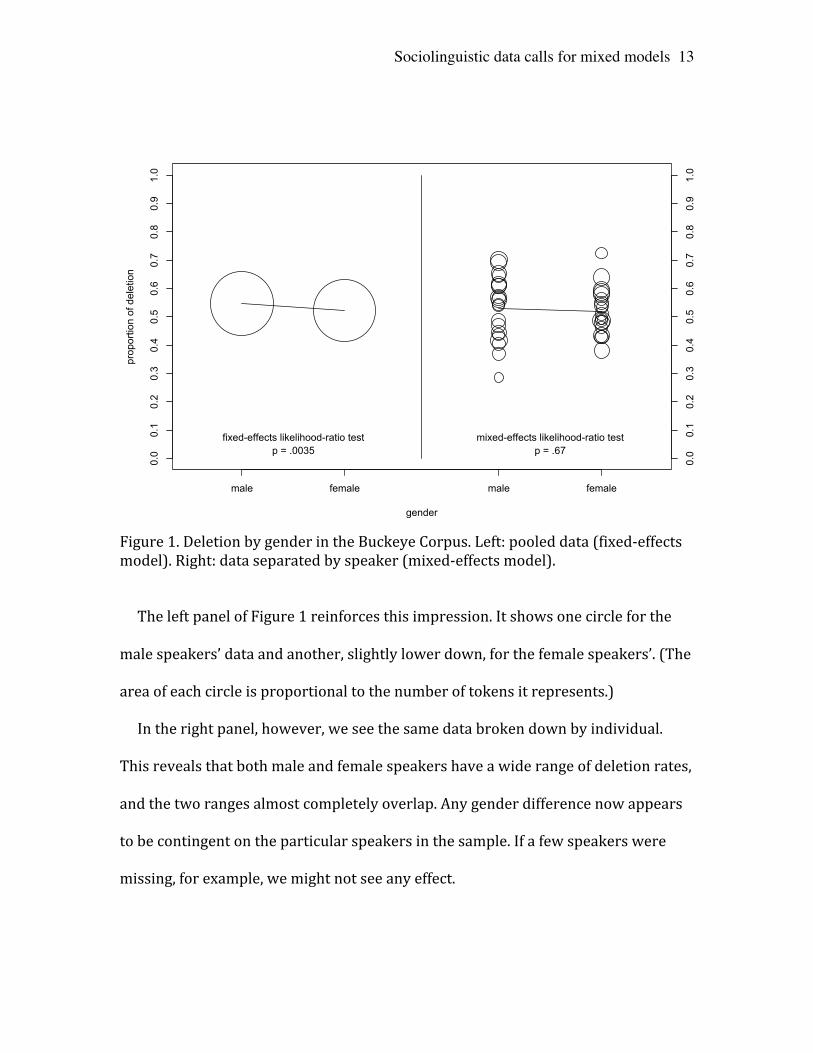
Figure 1. Deletion by gender in the Buckeye Corpus. Left: pooled data (fixed-‐effects model). Right: data separated by speaker (mixed-‐effects model).

The left panel of Figure 1 reinforces this impression. It shows one circle for the

male speakers’ data and another, slightly lower down, for the female speakers’. (The

area of each circle is proportional to the number of tokens it represents.)

In the right panel, however, we see the same data broken down by individual.

This reveals that both male and female speakers have a wide range of deletion rates,

and the two ranges almost completely overlap. Any gender difference now appears

to be contingent on the particular speakers in the sample. If a few speakers were

missing, for example, we might not see any effect.

gender

prop

ortio

n of

del

etio

n

0.0

0.1

0.2

0.3

0.4

0.5

0.6

0.7

0.8

0.9

1.0

0.0

0.1

0.2

0.3

0.4

0.5

0.6

0.7

0.8

0.9

1.0

male female male female

fixed-effects likelihood-ratio testp = .0035

mixed-effects likelihood-ratio testp = .67


14

We can formalize this by assessing the significance of gender by comparing

mixed-‐effects models having a subject intercept. Now the likelihood-‐ratio test

returns a p-‐value of 0.67, nowhere near the usual 0.05 threshold for statistical

significance. The mixed models say that while speakers vary, there is little evidence

for a gender difference. Even though we might have expected males to delete more,

as coronal stop deletion is a stable non-‐standard feature, this revised conclusion

accords better with the patterning of the speakers on Figure 1.

1B. Fixed-‐effects models inaccurately estimate the effect sizes of between-‐speaker

predictors, when some speakers contribute more data than others

In estimating a difference between two groups of speakers, we should ideally

treat each individual equally (“averaging by speaker”). Fixed-‐effects regression

distorts group differences by lumping the data from different individuals together

(“averaging by tokens”). Figure 2 helps to illustrate this distortion.


15

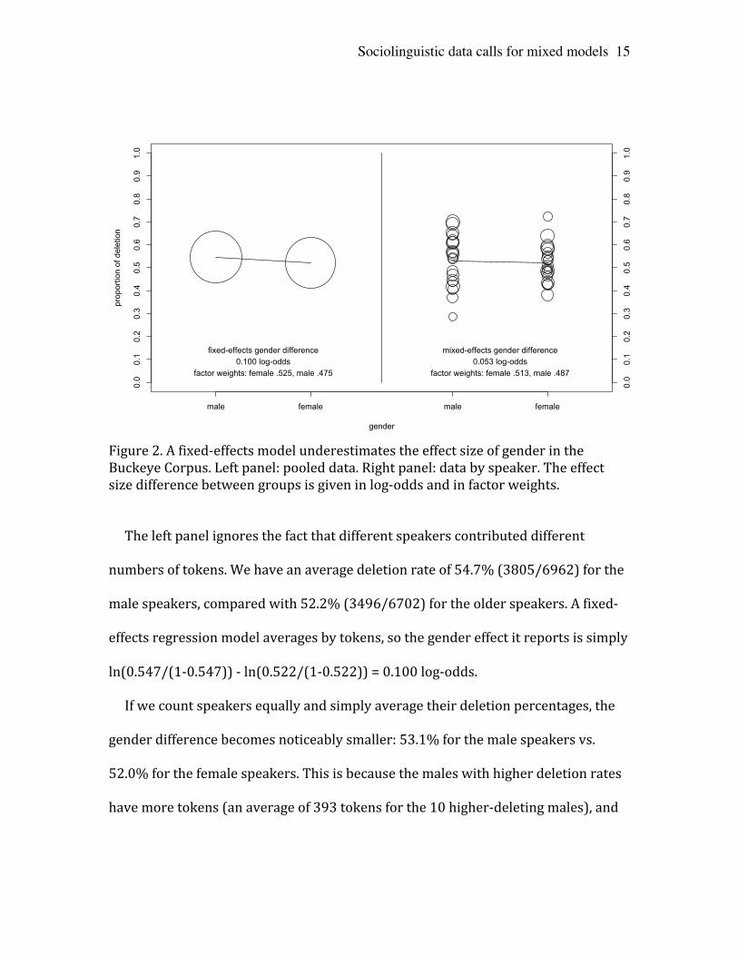
Figure 2. A fixed-‐effects model underestimates the effect size of gender in the Buckeye Corpus. Left panel: pooled data. Right panel: data by speaker. The effect size difference between groups is given in log-‐odds and in factor weights.

The left panel ignores the fact that different speakers contributed different

numbers of tokens. We have an average deletion rate of 54.7% (3805/6962) for the

male speakers, compared with 52.2% (3496/6702) for the older speakers. A fixed-‐

effects regression model averages by tokens, so the gender effect it reports is simply

ln(0.547/(1-‐0.547)) -‐ ln(0.522/(1-‐0.522)) = 0.100 log-‐odds.

If we count speakers equally and simply average their deletion percentages, the

gender difference becomes noticeably smaller: 53.1% for the male speakers vs.

52.0% for the female speakers. This is because the males with higher deletion rates

have more tokens (an average of 393 tokens for the 10 higher-‐deleting males), and

gender

prop

ortio

n of

del

etio

n

0.0

0.1

0.2

0.3

0.4

0.5

0.6

0.7

0.8

0.9

1.0

0.0

0.1

0.2

0.3

0.4

0.5

0.6

0.7

0.8

0.9

1.0

male female male female

fixed-effects gender difference0.100 log-odds

factor weights: female .525, male .475

mixed-effects gender difference0.053 log-odds

factor weights: female .513, male .487


16

the males with lower deletion rates have fewer tokens (an average of 303 tokens for

the 10 lower-‐deleting males). Averaging by tokens skews the male estimate higher.

In keeping with a more even treatment of speakers behind the averages, a mixed

model with a random speaker intercept returns a smaller – and as we saw in section

1A, a non-‐significant – gender difference. [Note 14] The mixed model effect size is

only about half as large: 0.053 log-‐odds.

The inaccuracy of fixed-‐effects models, faced with token imbalance, is a general

problem, but its direction can vary; here, the effect size was overestimated, but with

other data, a fixed-‐effects model could underestimate a between-‐speaker effect size.

Another example of overestimation is found in Becker (2009), working with a

data set of 3000 tokens of postvocalic /r/ from seven New York City speakers. Five

of the speakers are female and two are male. While this is too few speakers to

seriously estimate a population gender difference, the results illustrate our point.

In Becker’s data, the female speaker with the most data has the lowest rate of

postvocalic /r/, and the female with the least data has the highest rate of /r/. [Note

15a] Averaging by tokens, both of these women will act to boost the deletion rate for

their gender, in turn exaggerating the difference between women and men.

Fixed-‐effects models might be a viable option – at least as far as effect sizes are

concerned – if our data were always balanced, with equal numbers of tokens per

speaker (and per word). Such balance may be feasible in certain experimental

contexts, but sociolinguists’ desire to elicit conversational speech virtually ensures

that it will be rare in our data sets. We can limit imbalance artificially, by placing a

ceiling on the tokens from a given speaker or of a given word, but this approach


17

throws away valuable data arbitrarily and thus introduces its own problems. Mixed

models are preferable because they can accept our complete, complex data sets as

they are, working equally well if the data is balanced or unbalanced. [Note 16]

1C. Fixed-‐effects models inaccurately estimate the effect sizes of within-‐speaker

predictors, when speakers do not share the same balance of data

The discussion so far has revolved around the consequences of ignoring

individual-‐speaker variation as it relates to between-‐speaker predictors. Within-‐

speaker predictors, too, can be misestimated by failing to take speaker variation into

account. This would clearly be true if these predictors’ effects varied from speaker

to speaker, but is also the case if the variability applies only to speakers’ intercepts.

The issue involves another type of data imbalance. Looking at speech style, for

example, we would have cause for concern if different speakers were represented

by different amounts of data in different styles. Suppose we measure a vowel in

three styles; the number of reading passage and word list tokens is constant across

speakers, but the amount of spontaneous speech from each person is different.

Imagine further that the speakers who produce more spontaneous speech tend to

produce a lower F1 in all styles. Unless we model this, the group estimate for

spontaneous speech will be downwardly biased. The combination of speaker

variability and token imbalance will be mistaken for an effect of style. [Note 17]

Using a simulation, we can illustrate this point while assuming that speakers

“have the same grammar” – the speech styles affect each speaker in the same way.

Unlike real data, the population parameters of simulated data are known. We might


18

define our population to have no underlying difference between two groups.

Samples from the groups will usually show some difference, due to chance

(sampling error). By sampling many times, we can estimate how often the observed

difference exceeds a threshold, such as the level found in a real data set. Here,

simulations will be used to compare the parameter estimates made by fixed-‐effects

and mixed-‐effects models, each fit to the same samples drawn from the same

population.

We will simulate and model 1000 data sets. In each, there are 10 speakers, whose

intercepts differ: their average F1 values are normally distributed with a mean of

500 Hz and a standard deviation of 100 Hz. All speakers produce 50 tokens in word

list style and 50 tokens in reading passage style. For spontaneous speech, two

speakers produce 25 tokens, six produce 50 tokens, and two produce 75 tokens.

Within each style, each speaker’s F1 values vary randomly with a standard

deviation of 50 Hz. Between styles, all speakers differ in the same way. Compared to

their reading passage tokens, every speaker’s word list tokens are 50 Hz higher in

F1, and their spontaneous speech tokens are 50 Hz lower, on average. (This is for

the purpose of illustration rather than necessarily representing a plausible style

effect).

Where the data is balanced across speakers, the fixed-‐effects and mixed-‐effects

coefficients are unbiased and always nearly identical: close to 500 Hz for reading

passage, +50 Hz for word list. For the imbalanced spontaneous speech style, both

models are unbiased, with a mean effect near -‐50 Hz, but while the mixed model is

usually quite close to the mean, the fixed-‐effects coefficient varies widely. The


19

average difference between the estimates was 7.7 Hz; the largest difference was

32.8 Hz.

In a large majority of runs – 821 of 1000 – the mixed model estimate is closer to

the theoretical effect size of -‐50 Hz, by a median amount of 5.8 Hz. In the other 179

runs, it is the fixed-‐effect estimate that is closer to -‐50 Hz, by a median of 1.7 Hz.

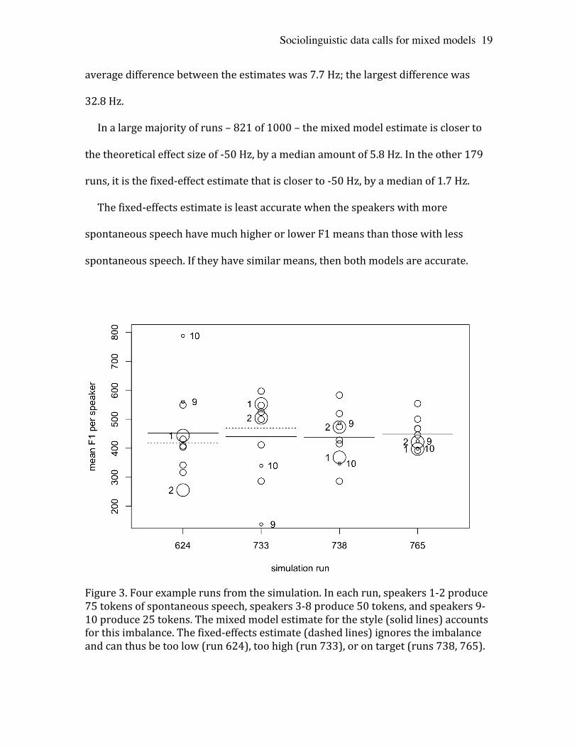
The fixed-‐effects estimate is least accurate when the speakers with more

spontaneous speech have much higher or lower F1 means than those with less

spontaneous speech. If they have similar means, then both models are accurate.

Figure 3. Four example runs from the simulation. In each run, speakers 1-‐2 produce 75 tokens of spontaneous speech, speakers 3-‐8 produce 50 tokens, and speakers 9-‐10 produce 25 tokens. The mixed model estimate for the style (solid lines) accounts for this imbalance. The fixed-‐effects estimate (dashed lines) ignores the imbalance and can thus be too low (run 624), too high (run 733), or on target (runs 738, 765).


20

Figure 3 shows how token imbalances affect four simulations. In run 624, the

position of the large and small circles makes the fixed-‐effects estimate for

spontaneous speech too low: -‐83 Hz. In run 733, the opposite configuration makes it

too high: -‐17 Hz. The imbalanced speakers do not have extreme means in run 738;

the estimate is -‐50 Hz. In run 765, all the imbalanced speakers are low, cancelling

each other out; the estimate is -‐49 Hz. The mixed model, on the other hand, is near -‐

50 Hz in all four cases.

Random token-‐level variation is the only reason why the mixed model sometimes

appears less accurate than the fixed-‐effects model, as occurred in 179 of 1000

simulations. No combination of data imbalance and intercept variation would cause

this to happen. Even here, the mixed model is not really less accurate. It always

models the observed grouped data better, but fluctuations in the sample may cause

the estimates to deviate from the parameters of a simulation or a real population.

1D. Fixed-‐effects models underestimate the effect sizes of within-‐speaker predictors

in logistic regression

With a binary linguistic variable, we cannot model the response probability as a

linear function of the predictors, at the risk of predicting probabilities outside the

legitimate range of 0 to 1. Instead, we typically model the log-‐odds of the response

probability, ln(p/(1-p)), a quantity that can range from -‐∞ to +∞.

But if we adopt logistic regression to analyze binary data, we should perhaps no

longer make comparisons by manipulating raw proportions in a linear way. If we

are committed to the log-‐odds scale, we should regard the difference between 50%


21

and 60% (0.41 log-‐odds) as being only half as large as the difference between 80%

and 90% (0.81 log-‐odds), contra, e.g. Guy (2007). [Note 18]

Do language users or language learners actually interpret proportions, and

differences of proportions, on the log-‐odds scale? Logistic regression is well

motivated for the study of diachronic change, because S-‐shaped curves are actually

observed for many changes in progress. Indeed, some simple theoretical

mechanisms of competition between variants (or grammars) predict that rates of

change should be proportional to p(1-p), ensuring that a plot of p against time is a

logistic curve (Kroch 1989, Yang 2000, Denison 2003).

For synchronic constraints, there is less evidence for the S-‐shaped patterns we

would expect to see if the log-‐odds of binary responses were affected linearly by

predictors. For example, within a speech community we do not generally find the

largest (raw) differences in linguistic production between the social classes in the

middle of the class hierarchy, with smaller differences between groups at either end

of the spectrum (Labov 1966). And turning to the perception of social class, it seems

unlikely that small (raw) differences near 0% or 100% would make as much of an

impression on listeners as larger differences in the vicinity of 50%.

Whether or not it is motivated in all sociolinguistic circumstances, logistic

regression is a convenient tool for modeling the constraints on binary variables.

Rather than discourage its use, the purpose of this section is to illustrate a pitfall in

applying fixed-‐effects logistic regression to grouped data.

Imagine that speaker A uses a variant 50% of the time in context “low” and 60%

in context “high”, a difference, as noted, of 0.41 log-‐odds. Speaker B uses the variant


22

much more overall – 80% of the time in context “low”, 86% in context “high” – but

the contextual difference is the same on the log-‐odds scale. From the point of view of

logistic regression, the high/low predictor has the same effect for both speakers.

They differ only in their overall use of the variant, that is to say, in their intercept.

However, if we combine data from speakers A and B, we will always observe a

high/low effect that is smaller than 0.41 log-‐odds. If A and B contribute equally, the

combined “low” context will show an overall rate of 65% (the average of 50% and

80%), and the “high” context will show a rate of 73% (the average of 60% and 86%).

This difference is only 0.37 log-‐odds, 9% smaller than the true effect size.

The intercept difference between speakers A and B is quite large here (1.39 log-‐

odds). The larger the individual-‐intercept variation, the worse a mistake it is to

estimate a within-‐speaker effect by pooling the data, which ends up averaging

speakers’ proportions on the probability scale instead of on the log-‐odds scale.

Table 1 shows the average effect size from a repeated simulation of 200 tokens

from each of 50 speakers. The data is divided equally into “high” and “low” groups,

and the underlying effect size is 1 log-‐odds unit. Speakers’ intercepts are normally

distributed with a standard deviation of 0 (no speaker variation), 0.5, 1, 1.5, or 2 log-‐

odds. (Admittedly, the higher values here may represent more variation than is

likely to be observed within a single speaker demographic.)

The table shows the average effect size, over 100 repetitions of the simulation,

from a fixed-‐effects model with “high/low” as the only predictor, and from a mixed

model that also includes a random speaker intercept. [Note 19]


23

speaker intercept variation standard deviation (log-‐odds)

fixed-‐effects model mean effect size (log-‐odds) response ~ high.low

mixed-‐effects model mean effect size (log-‐odds) response ~ high.low + (1|speaker)

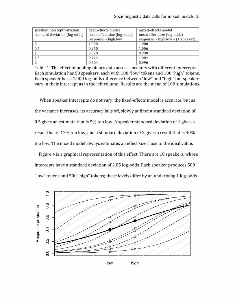
0 1.000 1.000 0.5 0.950 1.006 1 0.828 0.998 1.5 0.714 1.004 2 0.604 0.996 Table 1. The effect of pooling binary data across speakers with different intercepts. Each simulation has 50 speakers, each with 100 “low” tokens and 100 “high” tokens. Each speaker has a 1.000 log-‐odds difference between “low” and “high” but speakers vary in their intercept as in the left column. Results are the mean of 100 simulations.

When speaker intercepts do not vary, the fixed-‐effects model is accurate, but as

the variance increases, its accuracy falls off, slowly at first: a standard deviation of

0.5 gives an estimate that is 5% too low. A speaker standard deviation of 1 gives a

result that is 17% too low, and a standard deviation of 2 gives a result that is 40%

too low. The mixed model always estimates an effect size close to the ideal value.

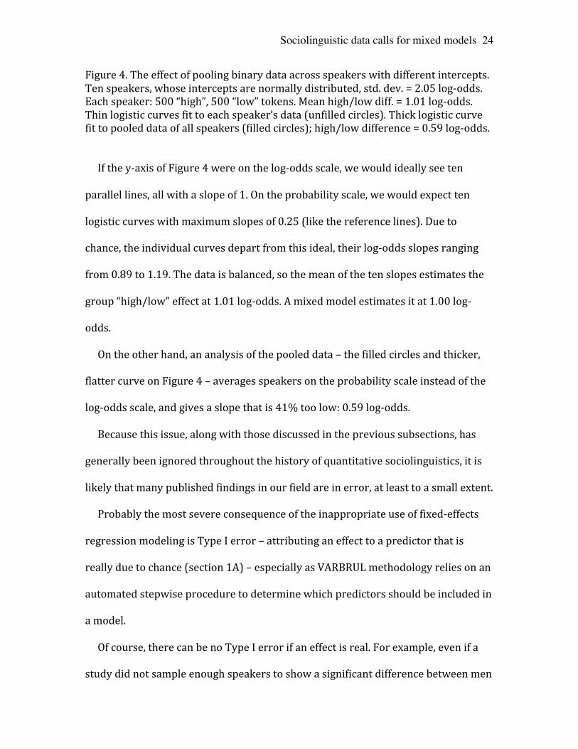
Figure 4 is a graphical representation of this effect. There are 10 speakers, whose

intercepts have a standard deviation of 2.05 log-‐odds. Each speaker produces 500

“low” tokens and 500 “high” tokens; these levels differ by an underlying 1 log-‐odds.


24

Figure 4. The effect of pooling binary data across speakers with different intercepts. Ten speakers, whose intercepts are normally distributed, std. dev. = 2.05 log-‐odds. Each speaker: 500 “high”, 500 “low” tokens. Mean high/low diff. = 1.01 log-‐odds. Thin logistic curves fit to each speaker’s data (unfilled circles). Thick logistic curve fit to pooled data of all speakers (filled circles); high/low difference = 0.59 log-‐odds.

If the y-‐axis of Figure 4 were on the log-‐odds scale, we would ideally see ten

parallel lines, all with a slope of 1. On the probability scale, we would expect ten

logistic curves with maximum slopes of 0.25 (like the reference lines). Due to

chance, the individual curves depart from this ideal, their log-‐odds slopes ranging

from 0.89 to 1.19. The data is balanced, so the mean of the ten slopes estimates the

group “high/low” effect at 1.01 log-‐odds. A mixed model estimates it at 1.00 log-‐

odds.

On the other hand, an analysis of the pooled data – the filled circles and thicker,

flatter curve on Figure 4 – averages speakers on the probability scale instead of the

log-‐odds scale, and gives a slope that is 41% too low: 0.59 log-‐odds.

Because this issue, along with those discussed in the previous subsections, has

generally been ignored throughout the history of quantitative sociolinguistics, it is

likely that many published findings in our field are in error, at least to a small extent.

Probably the most severe consequence of the inappropriate use of fixed-‐effects

regression modeling is Type I error – attributing an effect to a predictor that is

really due to chance (section 1A) – especially as VARBRUL methodology relies on an

automated stepwise procedure to determine which predictors should be included in

a model.

Of course, there can be no Type I error if an effect is real. For example, even if a

study did not sample enough speakers to show a significant difference between men


25

and women, the study’s estimate of the gender difference might not be useless,

especially if other studies corroborated the finding with similar results.

The idea that published effect sizes might be inaccurate (sections 1B-‐1D) is

troubling, but it is mitigated by the VARBRUL practice of not interpreting results in a

strongly quantitative way. Sociolinguists are usually content to say that the effect of

B is larger than that of A, rather than claiming that B has, say, 1.75 times the effect of

A. Studies making more direct use of a model’s numeric parameters, such as the

“exponential” account of coronal stop deletion (Guy 1991), are more open to

criticism if, for any of the reasons outlined, the numbers they rely on are inaccurate.

2. A comparison of ordinary fixed-‐effects (VARBRUL) and mixed-‐effects regression,

applied to coronal stop deletion in the Buckeye sub-‐corpus

The parameters of simulations are manipulated to make desired points clearly.

When we compare methodologies on real data sets, the differences are not always

as remarkable, and a given difference may have complex and multiple causes.

Again using the coronal stop deletion data from the Buckeye Corpus, this section

compares the results of a VARBRUL-‐style analysis to one employing mixed models.

Some of the resulting differences are subtle – especially in effect sizes – but taken

together they are substantial enough to recommend the mixed-‐model approach.

Six predictors will be examined: segment identity, preceding context, following

context, morphological category, word frequency, and gender. The coding and

ordering of phonological factors is based on Smith et al. (2009).


26

Segment identity is either /t/ or /d/. Preceding phonological segments fall into

five categories: sibilant, stop, nasal, non-‐sibilant fricate, and lateral (in decreasing

order of their usual deletion-‐favoring effect). Following segments also form five

groups: obstruent, liquide, glide, vowel, and pause (also in order, with the position

of pause being dialect-‐specific; Guy 1980).

Morphological category separates the regular past tense (e.g. missed) from the

irregular past tenses, a miscellaneous group (e.g. burnt, cost, held, left, sent, went).

The other two morphological categories are monomorphemes (e.g. cult) and -‐n’t.

Word frequency was calculated on the basis of 22.8 million words of telephone

speech (derived from the Fisher and Switchboard corpora by Kyle Gorman), taking

the base-‐10 logarithm of the ratio of the frequency of each wordform to that of the

median frequency word. This center point – canned, found 104 times – receives a

score of 0. A word one-‐tenth as frequent (like institutionalized) receives a score of -‐

1, a word 100 times as frequent (like friend) receives a score of +2, and so forth. The

most frequent words are don’t at +3.23 and just at +3.22; these two words make up

1.5% of the telephone corpus, and 29% of the coronal stop deletion corpus. All

words with the minimum frequency score of -‐2.02 (like annexed, nudist, or

whupped) occurred just once in the 22.8M-‐word corpus.

Excluding 46 tokens of words missing from the telephone corpus, and 17 tokens

without a clear following segment, left us with 13,601 tokens of 881 word types.

Our mixed models will employ random intercepts for word and speaker, because

we have between-‐word predictors (segment, preceding context, morphological


27

category, frequency) and a between-‐speaker predictor (gender). Note that following

context does not have a nesting relationship with word or speaker.

Without random slopes, we assume that speakers may vary in their overall level

of deletion, but have the same grammar with respect to the within-‐speaker

predictors. Individual words may favor or disfavor deletion, but the effects of

following segment and gender are assumed to be constant for each word type.

2A. Differences in significance

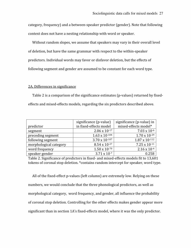
Table 2 is a comparison of the significance estimates (p-‐values) returned by fixed-‐

effects and mixed-‐effects models, regarding the six predictors described above.

predictor

significance (p-‐value) in fixed-‐effects model

significance (p-‐value) in mixed-‐effects model*

segment 2.06 x 10-‐17 7.03 x 10-‐6 preceding segment 1.63 x 10-‐104 1.70 x 10-‐29 following segment 3.70 x 10-‐107 1.87 x 10-‐112 morphological category 8.54 x 10-‐27 7.25 x 10-‐11 word frequency 1.50 x 10-‐70 2.16 x 10-‐4 speaker gender 3.71 x 10-‐7 0.258 Table 2. Significance of predictors in fixed-‐ and mixed-‐effects models fit to 13,601 tokens of coronal stop deletion. *contains random intercept for speaker, word type.

All of the fixed-‐effect p-‐values (left column) are extremely low. Relying on these

numbers, we would conclude that the three phonological predictors, as well as

morphological category, word frequency, and gender, all influence the probability

of coronal stop deletion. Controlling for the other effects makes gender appear more

significant than in section 1A’s fixed-‐effects model, where it was the only predictor.


28

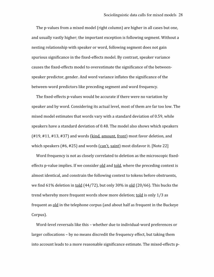
The p-‐values from a mixed model (right column) are higher in all cases but one,

and usually vastly higher; the important exception is following segment. Without a

nesting relationship with speaker or word, following segment does not gain

spurious significance in the fixed-‐effects model. By contrast, speaker variance

causes the fixed-‐effects model to overestimate the significance of the between-‐

speaker predictor, gender. And word variance inflates the significance of the

between-‐word predictors like preceding segment and word frequency.

The fixed-‐effects p-‐values would be accurate if there were no variation by

speaker and by word. Considering its actual level, most of them are far too low. The

mixed model estimates that words vary with a standard deviation of 0.59, while

speakers have a standard deviation of 0.48. The model also shows which speakers

(#19, #11, #13, #37) and words (kind, amount, front) most favor deletion, and

which speakers (#6, #25) and words (can’t, saint) most disfavor it. [Note 22]

Word frequency is not as closely correlated to deletion as the microscopic fixed-‐

effects p-‐value implies. If we consider old and told, where the preceding context is

almost identical, and constrain the following context to tokens before obstruents,

we find 61% deletion in told (44/72), but only 30% in old (20/66). This bucks the

trend whereby more frequent words show more deletion; told is only 1/3 as

frequent as old in the telephone corpus (and about half as frequent in the Buckeye

Corpus).

Word-‐level reversals like this – whether due to individual-‐word preferences or

larger collocations – by no means discredit the frequency effect, but taking them

into account leads to a more reasonable significance estimate. The mixed-‐effects p-‐


29

value near .0002 allows for a very small chance that the frequency effect is spurious.

The fixed-‐effects value near 10-‐70 is not compatible with the complexities of the data.

With a sufficiently large data set such as this one, real effects – and most of the

ones here have been detected in several previous studies – will remain significant

using mixed-‐effects regression. With fixed-‐effects regression, not only are non-‐

significant predictors called significant, the significance of real predictors is

exaggerated.

2B. Differences in effect sizes

Moving beyond significance levels – which are highly dependent on the size of a

data set, as well as on the strength of the effects – this section will compare the

estimated effect sizes between a fixed-‐effects and a mixed-‐effects model, each of

which contain the five predictors that were confirmed by the mixed-‐effects model

above as significant (that is, all of them except gender).

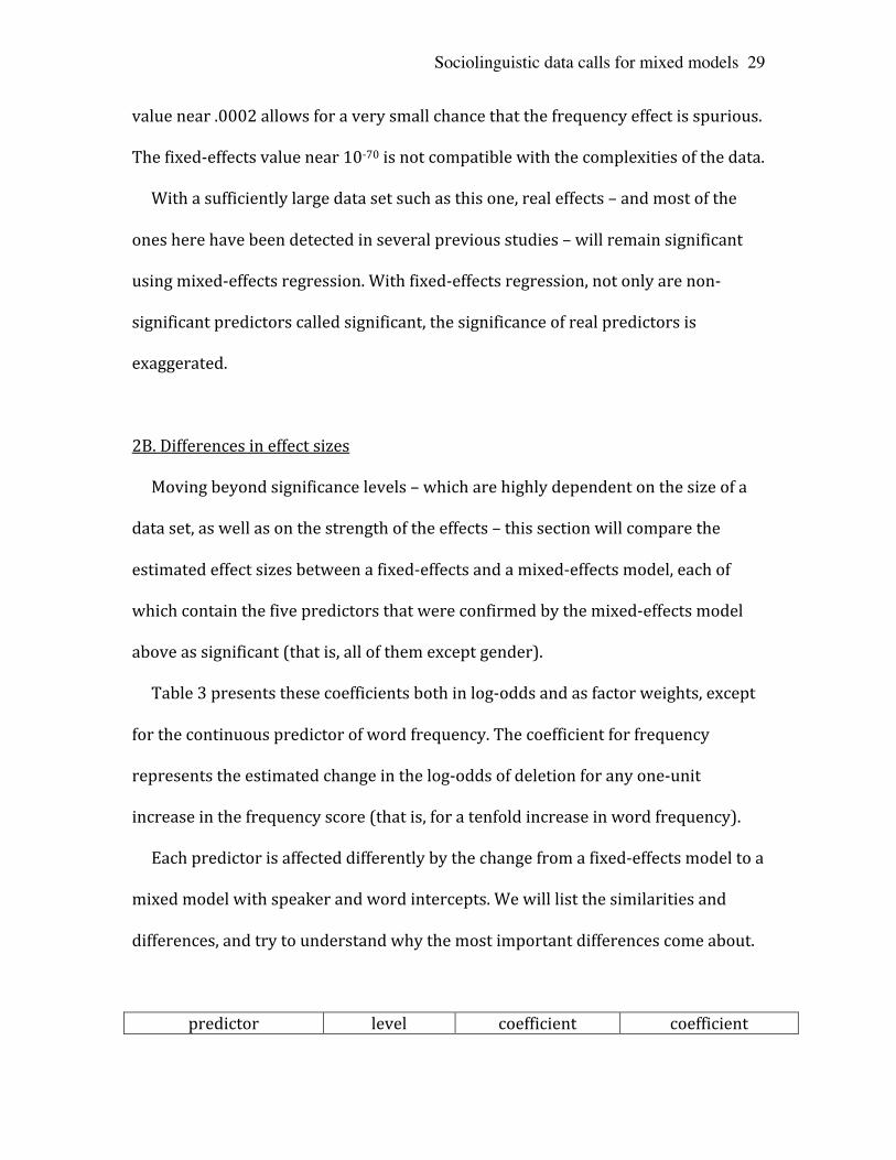
Table 3 presents these coefficients both in log-‐odds and as factor weights, except

for the continuous predictor of word frequency. The coefficient for frequency

represents the estimated change in the log-‐odds of deletion for any one-‐unit

increase in the frequency score (that is, for a tenfold increase in word frequency).

Each predictor is affected differently by the change from a fixed-‐effects model to a

mixed model with speaker and word intercepts. We will list the similarities and

differences, and try to understand why the most important differences come about.

predictor level coefficient coefficient


30

(factor group) (factor) (factor weight) in fixed-‐effects model

(factor weight) in mixed-‐effects model*

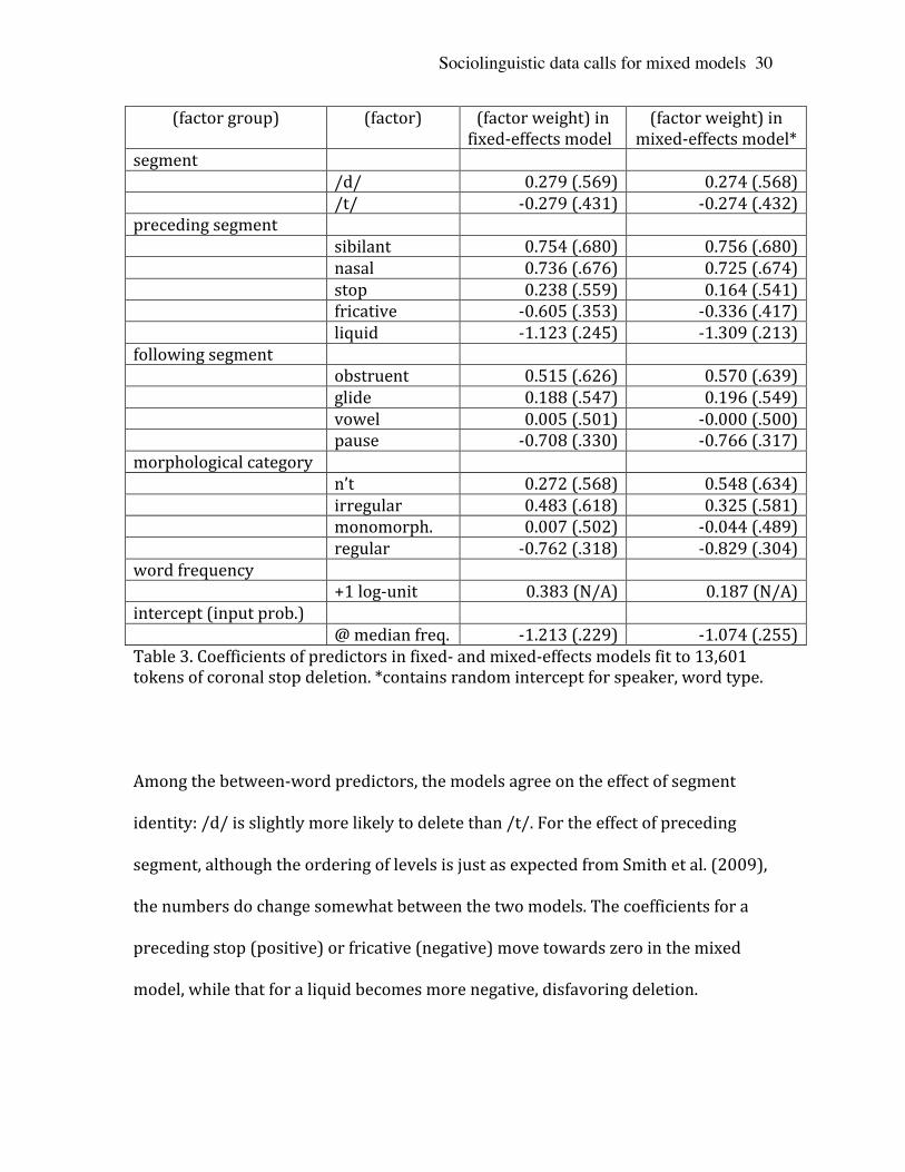
segment /d/ 0.279 (.569) 0.274 (.568) /t/ -‐0.279 (.431) -‐0.274 (.432) preceding segment sibilant 0.754 (.680) 0.756 (.680) nasal 0.736 (.676) 0.725 (.674) stop 0.238 (.559) 0.164 (.541) fricative -‐0.605 (.353) -‐0.336 (.417) liquid -‐1.123 (.245) -‐1.309 (.213) following segment obstruent 0.515 (.626) 0.570 (.639) glide 0.188 (.547) 0.196 (.549) vowel 0.005 (.501) -‐0.000 (.500) pause -‐0.708 (.330) -‐0.766 (.317) morphological category n’t 0.272 (.568) 0.548 (.634) irregular 0.483 (.618) 0.325 (.581) monomorph. 0.007 (.502) -‐0.044 (.489) regular -‐0.762 (.318) -‐0.829 (.304) word frequency +1 log-‐unit 0.383 (N/A) 0.187 (N/A) intercept (input prob.) @ median freq. -‐1.213 (.229) -‐1.074 (.255) Table 3. Coefficients of predictors in fixed-‐ and mixed-‐effects models fit to 13,601 tokens of coronal stop deletion. *contains random intercept for speaker, word type.

Among the between-‐word predictors, the models agree on the effect of segment

identity: /d/ is slightly more likely to delete than /t/. For the effect of preceding

segment, although the ordering of levels is just as expected from Smith et al. (2009),

the numbers do change somewhat between the two models. The coefficients for a

preceding stop (positive) or fricative (negative) move towards zero in the mixed

model, while that for a liquid becomes more negative, disfavoring deletion.


31

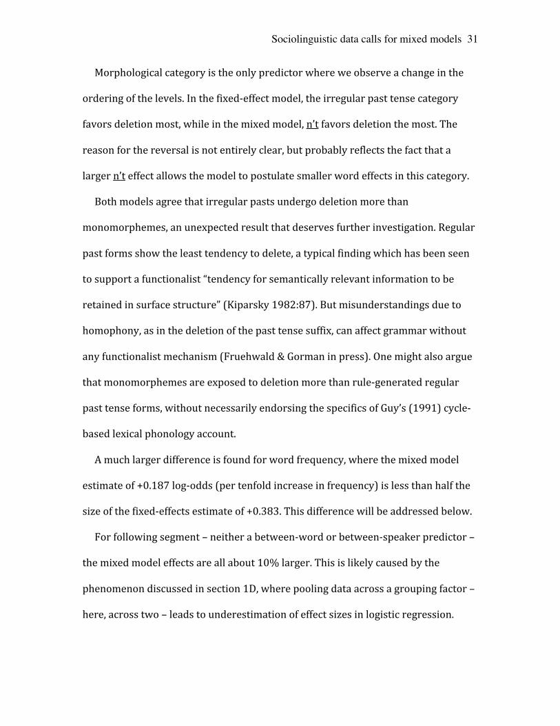
Morphological category is the only predictor where we observe a change in the

ordering of the levels. In the fixed-‐effect model, the irregular past tense category

favors deletion most, while in the mixed model, n’t favors deletion the most. The

reason for the reversal is not entirely clear, but probably reflects the fact that a

larger n’t effect allows the model to postulate smaller word effects in this category.

Both models agree that irregular pasts undergo deletion more than

monomorphemes, an unexpected result that deserves further investigation. Regular

past forms show the least tendency to delete, a typical finding which has been seen

to support a functionalist “tendency for semantically relevant information to be

retained in surface structure” (Kiparsky 1982:87). But misunderstandings due to

homophony, as in the deletion of the past tense suffix, can affect grammar without

any functionalist mechanism (Fruehwald & Gorman in press). One might also argue

that monomorphemes are exposed to deletion more than rule-‐generated regular

past tense forms, without necessarily endorsing the specifics of Guy’s (1991) cycle-‐

based lexical phonology account.

A much larger difference is found for word frequency, where the mixed model

estimate of +0.187 log-‐odds (per tenfold increase in frequency) is less than half the

size of the fixed-‐effects estimate of +0.383. This difference will be addressed below.

For following segment – neither a between-‐word or between-‐speaker predictor –

the mixed model effects are all about 10% larger. This is likely caused by the

phenomenon discussed in section 1D, where pooling data across a grouping factor –

here, across two – leads to underestimation of effect sizes in logistic regression.


32

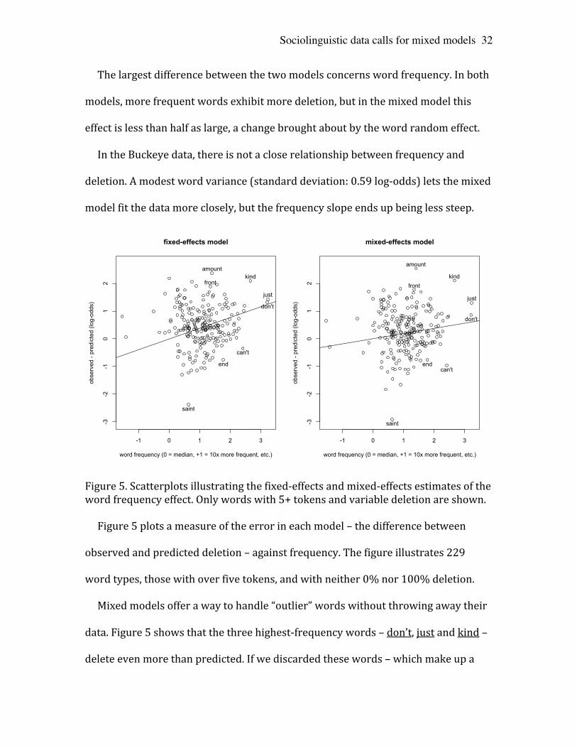
The largest difference between the two models concerns word frequency. In both

models, more frequent words exhibit more deletion, but in the mixed model this

effect is less than half as large, a change brought about by the word random effect.

In the Buckeye data, there is not a close relationship between frequency and

deletion. A modest word variance (standard deviation: 0.59 log-‐odds) lets the mixed

model fit the data more closely, but the frequency slope ends up being less steep.

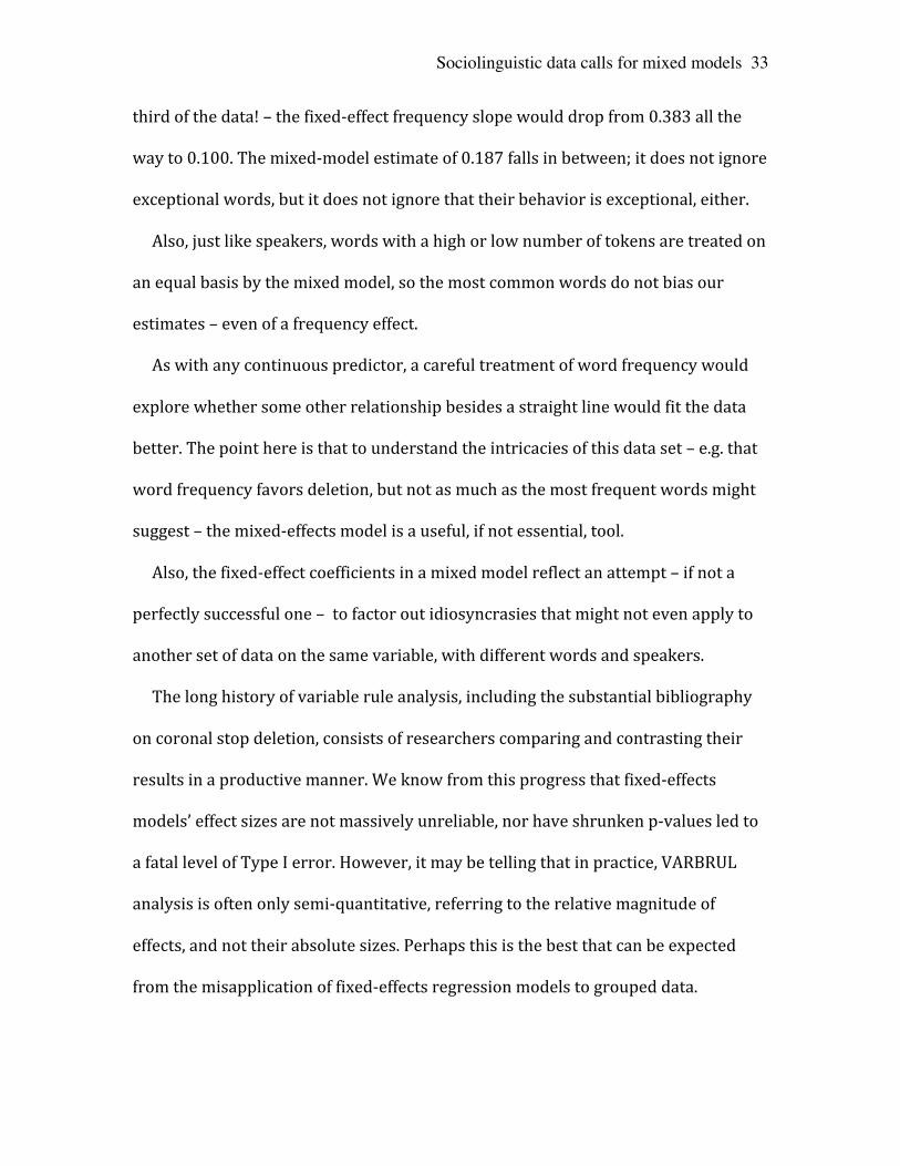
Figure 5. Scatterplots illustrating the fixed-‐effects and mixed-‐effects estimates of the word frequency effect. Only words with 5+ tokens and variable deletion are shown. Figure 5 plots a measure of the error in each model – the difference between

observed and predicted deletion – against frequency. The figure illustrates 229

word types, those with over five tokens, and with neither 0% nor 100% deletion.

Mixed models offer a way to handle “outlier” words without throwing away their

data. Figure 5 shows that the three highest-‐frequency words – don’t, just and kind –

delete even more than predicted. If we discarded these words – which make up a

-1 0 1 2 3

-3-2

-10

12

fixed-effects model

word frequency (0 = median, +1 = 10x more frequent, etc.)

obse

rved

- pr

edic

ted

(log-

odds

)

kind

don't

just

front

can't

end

amount

saint

-1 0 1 2 3

-3-2

-10

12

mixed-effects model

word frequency (0 = median, +1 = 10x more frequent, etc.)

obse

rved

- pr

edic

ted

(log-

odds

)

kind

don't

just

front

can'tend

amount

saint


33

third of the data! – the fixed-‐effect frequency slope would drop from 0.383 all the

way to 0.100. The mixed-‐model estimate of 0.187 falls in between; it does not ignore

exceptional words, but it does not ignore that their behavior is exceptional, either.

Also, just like speakers, words with a high or low number of tokens are treated on

an equal basis by the mixed model, so the most common words do not bias our

estimates – even of a frequency effect.

As with any continuous predictor, a careful treatment of word frequency would

explore whether some other relationship besides a straight line would fit the data

better. The point here is that to understand the intricacies of this data set – e.g. that

word frequency favors deletion, but not as much as the most frequent words might

suggest – the mixed-‐effects model is a useful, if not essential, tool.

Also, the fixed-‐effect coefficients in a mixed model reflect an attempt – if not a

perfectly successful one – to factor out idiosyncrasies that might not even apply to

another set of data on the same variable, with different words and speakers.

The long history of variable rule analysis, including the substantial bibliography

on coronal stop deletion, consists of researchers comparing and contrasting their

results in a productive manner. We know from this progress that fixed-‐effects

models’ effect sizes are not massively unreliable, nor have shrunken p-‐values led to

a fatal level of Type I error. However, it may be telling that in practice, VARBRUL

analysis is often only semi-‐quantitative, referring to the relative magnitude of

effects, and not their absolute sizes. Perhaps this is the best that can be expected

from the misapplication of fixed-‐effects regression models to grouped data.


34

Having described several clear advantages of applying mixed-‐effects models to

sociolinguistic data, this article recommends crossed random intercepts (at least) to

capture the effects of the individual speaker and individual word. Simulations using

known population parameters have shown how inaccurate our regression estimates

can be if we ignore the real structure of our data and model it as if each token were

independent and of equal value in determining the effects of the predictors.

A large corpus of coronal stop deletion provided a test case showing the

sometimes substantial differences in effect size, and the usually quite large and

important differences in statistical significance that are found between fixed-‐effects

and mixed models. The true parameters underlying any real data set are unknown,

but the observed differences can be understood with the insights taken from the

simulated examples.

Given enough data to fit it, a mixed-‐effects regression model will do a better job of

exposing spurious effects, while real effects will remain significant. Mixed models

also estimate effect sizes more accurately, in a way that abstracts from the

idiosyncrasies of the sample at hand. They offer more hope for truly quantitative

analysis and comparison with (or replication of) other research. If there is to be a

scientific sociolinguistics, mixed-‐effects regression will be one of its instruments.

Notes

1. There is some variation in the terminology used to discuss regression

models. The response can also be known as the dependent variable, with the

predictors known as independent variables. Predictors that are categorical


35

(having two or more discrete levels) are also called factors, but in the

VARBRUL literature they are called factor groups, with the individual levels

known as factors. When the coefficients for factors in a logistic regression are

reported on a 0-‐to-‐1 probability scale, they are called factor weights.

Similarly, the intercept becomes the corrected mean or input probability.

Ordinary fixed-‐effects models have also been called flat, while mixed-‐effects

or just mixed models are also known as hierarchical or multilevel models.

2. When the response is a count of occurrences rather than repetitions of a

choice, the best option may be log-‐linear (or Poisson) regression, where the

logarithm of the response variable is modeled as a linear function of the

predictors. Another possibility for count data is negative binomial regression

(Coxe et al. 2009).

3. The use of stepwise regression – the up-‐and-‐down procedure at the heart of

most VARBRUL analyses – is no longer recommended (Harrell 2001).

Another problem arises if predictors are highly correlated, when regression

coefficients become unreliable. Such multicollinearity among non-‐nested

predictors calls for other approaches (Chatterjee & Hadi 2006).

4. Another challenge for modeling linguistic data is autocorrelation: generally

speaking, this is the tendency for nearby tokens (in time or in space!) to

resemble each other. Autocorrelation can be handled within a mixed-‐effects

regression approach, but this will not be demonstrated in this article.

5. The VARBRUL-‐era dichotomy of internal (or linguistic) vs. external (or

social) factors is incomplete. Speech style can affect a response similarly to a


36

social factor like class (Labov 1966), but structurally it is quite different.

Speaker is nested within social class (each speaker belongs to only one class),

but not within style (each speaker uses several speech styles). A better

typology distinguishes among speaker-‐nesting (between-‐speaker), word-‐

nesting (between-‐word), and non-‐nesting (within-‐speaker, within-‐word)

predictors. The same predictor can play different roles. In a community

study, age is a between-‐speaker predictor. But in a longitudinal study, each

speaker produces data at several ages, so age is a within-‐speaker predictor.

6. Strictly speaking, a random effect is a factor whose levels are a randomly-‐

sampled subset of a larger population. Modeling random effects allows

inferences to be made about that population. If we sample 100 speakers to

represent a city, and include a random intercept (and perhaps random

slopes) for speaker, our results will apply – bearing in mind the appropriate

confidence intervals – to the whole population of the city. But if we study the

five children in a family, there is no population to generalize to. In this case, a

fixed effect for speaker will fit the sample data more closely. But if we wish to

model between-‐speaker predictors, speaker must always be a random effect.

7. [note deleted]

8. [note deleted]

9. A reviewer has suggested that a normally-‐distributed intercept for speaker is

more likely than the same thing for word. This suggests not that a word

intercept is unnecessary, but that we are further from accounting for the

other factors that make words behave differently. If observed word effects


37

are roughly normally distributed, it makes more sense to model them with a

random effect than to ignore them. Still, it is worth noting that an intercept

for word is more controversial than one for speaker (Guy 2009).

10. [note deleted]

11. [note deleted]

12. A regression model estimates k-1 parameters for a factor with k levels.

There are two common ways of reporting these parameters. In treatment

contrasts, one level is the baseline, with a coefficient of zero that is usually

not reported. The other k-1 coefficients represent the differences between

the baseline and each of the other levels. The intercept represents the

prediction for the cell where all factors have their baseline values.

With zero-‐sum or sum contrasts, the intercept is the grand mean of the

predictions for all cells. Each coefficient represents the deviation of one

group from the mean. Because the deviations for a factor sum to zero, one

coefficient is predictable from the others, and is usually not reported.

VARBRUL uses sum contrasts, and does report k coefficients for a factor with

k levels. Another VARBRUL particularity is that instead of log-‐odds units,

coefficients are reported as factor weights on the 0-‐to-‐1 probability scale.

13. [note deleted]

14. Especially in logistic regression, if a speaker had very few tokens, it would

not make sense to include their observed rate in a group average; the

estimate would be too unreliable. This is of most concern if a speaker has

fewer than about 50 tokens. Speaker #6 shows 45 deletions out of 157 total


38

tokens; we can report a 95% confidence interval for this proportion as 22%-‐

36%. So the estimate of 29% is not very precise, but not too imprecise either.

Mixed models use shrinkage to take into account the amount of data from

each speaker, adjusting those with less data towards the group mean.

15. A reviewer notes that the association between less data and more post-‐

vocalic /r/ may be no coincidence, as interviewees who feel uncomfortable

being recorded could produce more formal variants, yet fewer of them.

16. It is sometimes claimed that VARBRUL handles unbalanced data well

(Cedergren & Sankoff 1974), but this statement must be taken in context.

True, compared to other software available in that era, VARBRUL could

accept unbalanced data sets and fit regression models to them. However, the

coefficients of such fixed-‐effects models will be inaccurate when the data is

unbalanced, unless there is no speaker-‐level or word-‐level variation.

17. “Fixed-‐effects model” should be understood to refer to models without

predictors for grouping factors such as individual speaker. If there are no

between-‐speaker predictors, we can treat speaker as a fixed effect. We might

then automatically group speakers (Rousseau & Sankoff 1978b), or extract

demographic generalizations by performing non-‐parametric tests (Sigley

1997) or linear regression (Sankoff 2004) on the speaker effects. Because we

usually want to make inferences over a larger population of speakers than

those in our particular sample, a mixed model estimating speaker and

between-‐speaker effects simultaneously is generally to be preferred.


39

18. Differences between 0% and 10% or 90% and 100% are infinite in log-‐odds.

However, categorical behavior of 0% and 100% is perceived and produced,

even though it cannot be modeled elegantly using logistic regression.

19. For this simple type of simulation, an ordinary regression model with a fixed

effect for speaker yields almost identical results to a mixed model with a

random effect for speaker. As noted, it is only the absence of between-‐

speaker predictors that makes the speaker-‐as-‐fixed-‐effect option possible.

The fixed-‐effects model would be preferred if we were mainly interested in

these particular speakers. To control for speaker variation and make a

general estimate of within-‐speaker effects, the mixed model is preferred.

20. [note deleted]

21. [note deleted]

22. The words with the most “overdeletion” are kind, amount, and front, with

deletion rates of 87%, 83%, and 77%. Subtracting the random word effects,

our model predicts 49%, 31%, and 44% deletion for these words, relatively

low rates reflecting, in part, that the following segment is usually a vowel.

These words usually occur in collocations with of: kind is almost always kind

of, amount is almost always amount of, and front is in front of more than half

the time. How this relates to coronal stop deletion is unclear: the adverbial

kind of is plausibly its own lexical item, as is (arguably) in front of, but

certainly not amount of. It seems likely that prosody plays a role, as these

syllables are stressed and precede unstressed of. We could refine our model

by incorporating prosodic predictors into the fixed effects (see Sigley 2003).


40

There is other evidence for true lexical effects. Even though it often

appears as end of – in the same phonological and prosodic environment as

kind of – the word end is an “underdeleter,” with a predicted deletion rate of

52% but an observed rate of only 28%. The word can’t underdeletes even

more: predicted 68%, observed 36%. Can’t is interesting because deletion

can cause homophony with can, and a particularly undesirable homophony

at that, since the words are antonyms. The question of how actively speakers

avoid homonymy has been debated throughout the history of linguistics.

A somewhat cynical alternative is that the Buckeye Corpus speakers

actually deleted a normal amount in can’t, but that some of these tokens were

mistaken for can, apparently lowering the deletion rate. Another possibility

is that this type of mishearing – called leakage by Fruehwald and Gorman (in

press) – can, over time, change the probabilities of rule application.

Finally, we note a proposal by Guy (2007:112), in which overdeleting

words are given two phonological representations. For and, we would have

an /ænd/ that undergoes deletion normally, and a synonymous /æn/

accounting for the “overdeletion”. Despite raising theoretical and learnability

concerns, Guy’s theory makes two clear predictions. One is that there should

be no examples of underdeleting words. The other is that predictors like

following context should show a smaller effect on the exceptional words.

Against the first claim, we have already mentioned can’t and end; another

substantial underdeleter is aren’t: predicted 59% deletion, observed 35%.

We can test the following-‐context prediction by modeling three subsets of


41

the data: 171 overdeleting words (word effect above +0.2), 583 average

words (between -‐0.2 and +0.2), and 127 underdeleting words (below -‐0.2).

These three models estimate the deletion-‐favoring effect of a following

obstruent vs. a following vowel as 0.447 log-‐odds for the underdeleting

words, 0.568 for the average words, and 0.591 for the overdeleting words.

This interaction is neither significant (p = .11) nor in the predicted direction.

Even and only shows a reduced effect of following obstruent vs. vowel if

we use raw deletion percentages instead of their equivalents in log-‐odds.

Drawing from Neu (1980), Guy reports that ordinary words have 39.3%

deletion before obstruents, 15.8% before vowels. For and, it is 95.7% before

obstruents, 82.1% before vowels. Guy analyzes the range of percentages,

which is 0.58 times as large for and. But expressed in log-‐odds, the effect for

and is 1.28 times as large. Guy’s reasoning depends on rejecting the logistic

framework in favor of an older “multiplicative model of constraint effects.”

But even within Guy’s own framework, there is an inconsistency. The

following-‐segment range for and is 0.58 times as large as for ordinary words,

which implies a mixture of 58% underlying variable /ænd/ and 42%

invariant /æn/. But with this mix, we would predict that and should show .58

* .393 + .42 * 1 = 64.8% deletion before obstruents and .58 * .158 + .42 * 1 =

51.3% deletion before vowels. The observed deletion rates for and are far

higher: 95.7% and 82.1%. The algebraic trick simply does not work.

References


42

Bates, Douglas M. To appear. lme4: Mixed-‐effects modeling with R. New York:

Springer.

Bayley, Robert. 2002. The quantitative paradigm. In Chambers, J.K, Peter Trudgill

and Natalie Schilling-‐Estes (eds.), The handbook of language variation and

change. Oxford: Blackwell. 117-‐41.

Becker, Kara. 2009. /r/ and the construction of place identity on New York City’s

Lower East Side. Journal of Sociolinguistics 13(5): 634-‐658.

Cedergren, Henrietta J. and David Sankoff. 1974. Variable rules: performance as a

statistical reflection of competence. Language 50(2): 333-‐355.

Chatterjee, Samprit and Ali S. Hadi. 2006. Regression Analysis by Example. Fourth

edition. New York: Wiley.

Cox, David R. 1958. The regression analysis of binary sequences. Journal of the Royal

Statistical Society, Series B (Methodological) 20(2): 215–242.

Coxe, Stefany, Stephen G. West and Leona S. Aiken. 2009. The analysis of count data:

a gentle introduction to Poisson regression and its alternatives. Journal of

Personality Assessment 91(2): 121-‐136.

Denison, David. 2003. Log(ist)ic and simplistic S-‐curves. In Raymond Hickey (ed.),

Motives for language change. Cambridge: Cambridge University Press.

Fruehwald, Josef. 2008. Evaluation and simulation of exemplar-‐theoretic -‐t/-‐d

deletion. Paper presented at NWAV 37, Rice University, Houston.

Fruehwald, Josef and Kyle Gorman. In press. Cross-‐derivational feeding is

epiphenomenal. Studies in the Linguistic Sciences.


43

Gorman, Kyle. 2009. On VARBRUL – or, The Spirit of ’74. Unpublished manuscript.

http://ling.auf.net/lingBuzz/001080.

Guy, Gregory R. 1980. Variation in the group and the individual: the case of final stop

deletion. In William Labov (ed.), Locating language in time and space. New

York: Academic Press. 1-‐36.

Guy, Gregory R. 1991. Explanation in variable phonology: an exponential model of

morphological constraints. Language Variation and Change 3(1): 1-‐22.

Guy, Gregory R. 2007. Lexical exceptions in variable phonology. In Toni Cook and

Keelan Evanini (eds.) University of Pennsylvania Working Papers in Linguistics

13(2). 109-‐119.

Guy, Gregory R. 2009. GoldVarb: still the gold standard. Paper presented at NWAV

38, University of Ottawa.

Harrell, Frank E. 2001. Regression modeling strategies. New York: Springer.

Harrell, Frank E. 2010. Information allergy. Paper presented at USER!2010, NIST,

Gaithersburg, MD. http://blip.tv/file/3994546

Hooper, Joan Bybee. 1976. Word frequency in lexical diffusion and the source of

morphophonological change. In William Christie (ed.), Current progress in

historical linguistics. Amsterdam: North Holland. 95-‐105.

Johnson, Daniel E. 2009. Getting off the GoldVarb standard: introducing Rbrul for

mixed-‐effects variable rule analysis. Language and Linguistics Compass 3(1):

359-‐383.

Kiparsky, Paul. 1982. Explanation in phonology. Dordrecht: Foris.


44

Kroch, Tony. 1989. Reflexes of grammar in patterns of language change. Language

Variation and Change 1: 199-‐244.

Labov, William. 1966. The social stratification of English in New York City.

Washington DC: Center for Applied Linguistics.

Lemon, Jim. 2009. On the perils of categorizing responses. Tutorials in Quantitative

Methods for Psychology 5(1): 35-‐39.

Neu, Helene, 1980. Ranking of constraints on –t,d deletion in American English. In

William Labov (ed.), Locating language in time and space. New York: Academic

Press. 37–54.

Pierrehumbert, Janet. 2001. Exemplar dynamics: word frequency, lenition and

contrast. In Joan Bybee and Paul Hopper (eds.), Frequency and the emergence

of linguistic structure. Philadelphia: John Benjamins.

Pinheiro, José C. and Douglas M. Bates. 2000. Mixed-‐effects models in S and S-‐PLUS.

New York: Springer.

Pitt, M. A., Dilley, L., Johnson, K., Kiesling, S., Raymond, W., Hume, E. and Fosler-‐

Lussier, E. 2007. Buckeye Corpus of Conversational Speech (2nd release).

Columbus OH: Department of Psychology, Ohio State University.

Rousseau, Pascale and David Sankoff. 1978a. Advances in variable rule

methodology. In David Sankoff (ed.), Linguistic variation: models and methods.

New York: Academic. 57-‐69.

Rousseau, Pascale and David Sankoff. 1978b. A solution to the problem of grouping

speakers. In David Sankoff (ed.), Linguistic variation: models and methods.

New York: Academic. 97-‐117.


45

Royston, Patrick, Douglas G. Altman and Willi Sauerbrei. 2006. Dichotomizing

continuous predictors in multiple regression: a bad idea. Statistics in medicine

25: 127-‐141.

Sankoff, David and Suzanne Laberge. 1978. Statistical dependencies among

successive occurrences of a variable in discourse. In David Sankoff (ed.),

Linguistic variation: models and methods. New York: Academic. 119-‐126.

Sankoff, David. 2004. Variable rules. In Ulrich Ammon et al. (eds.), Sociolinguistics:

an international handbook of the science of language and society. 2nd edition.

Berlin: Walter de Gruyter. 1150-‐63.

Sigley, Robert. 1997. Choosing your relatives: relative clauses in New Zealand

English. Ph.D. thesis, Victoria University of Wellington.

Sigley, Robert. 2003. The importance of interaction effects. Language variation and

change 15(2): 227-‐253.

Smith, Jennifer, Mercedes Durham and Liane Fortune. 2009. Universal and dialect-‐

specific pathways of acquisition: caregivers, children, and t/d deletion.

Language Variation and Change 21(1): 69-‐95.

Tagliamonte, Sali A. 2006. Analysing sociolinguistic variation. Cambridge:

Cambridge University Press.

Yang, Charles D. 2000. Internal and external forces in language change. Language

variation and change 12(3): 231-‐250.

Zipf, George K. 1935. Human Behavior and the Principle of Least-‐Effort. Cambridge

MA: Addison-‐Wesley.

Sociolinguistic data calls for mixed models 1 · Sociolinguistic data calls for mixed models 2!...

Documents

Transcript of Sociolinguistic data calls for mixed models 1 · Sociolinguistic data calls for mixed models 2!...