Socioeconomic Success and Health in Later Life:

Evidence from the Indonesia Family Life Survey

Firman Witoelar World Bank

John Strauss

University of Southern California

Bondan Sikoki Survey Meter

September, 2009

Paper to be presented at the International Union for the Scientific Study of Population

International Population Conference October 2009, Marrakesh, Morocco

An earlier version of this paper was presented at the Annual Meetings of the Population Association of America, April, 2009, Detroit. We thank Paul Heaton, James P Smith and other participants of the RAND Labor and Population Workshop for their very helpful comments. The views expressed here do not necessarily reflect those of the World Bank and of its member countries. All errors are ours.

Abstract

Indonesia has been undergoing a major health and nutrition transition over the past twenty or more years and there has begun a significant aging of the population as well. In this paper we focus on documenting major changes in the health of the population aged 45 years and older, since 1993. We use the Indonesia Family Life Survey (IFLS), a large-scale, broad-based panel survey of households and individuals, covering 4 full waves from 1993 to 2007/8. Much of the changes can be seen as improvements in health, such as the movement out of undernutrition and communicable disease as well as the increasing levels of hemoglobin. On the other hand, other changes such as the increase in overweight and waist circumference, especially among women, and continuing high levels of hypertension that seems to be inadequately addressed by the health system, indicate that the elderly population in Indonesia is increasingly exposed to higher risk factors that are correlated with chronic problems such as cardiovascular diseases and diabetes. In addition to documenting long-run changes in health and its distribution among the elderly Indonesian population, we examine correlations between socio-economic status, principally education and percapita expenditure, and numerous health outcome and behavioral variables. We find generally strong correlations between our health variables and SES and find in particular, the schooling plays a role in reducing the adverse health effects of aging. We also find that for hypertension in particular, that there is a very large degree of underdiagnosis in this population, one that is weakly correlated with SES. This result raises serious questions regarding the ability of the health system in Indonesia to cope with the rapid aging of the population and the transition from infectious to chronic diseases.

1 

 

1. Introduction

Indonesia has been undergoing a health and nutrition transition over the past 20 years and more.

Overall, health of the population has been improving, as indicated by a continuing rise in

attained adult heights for men and women over the entire 20th century (heights of both men and

women have been increasing by about 1 cm per decade over this period, Strauss and Thomas,

1995; Strauss et al, 2004a).  In Indonesia, infectious diseases caused 72 percent of all deaths in

1980; by 1992, just over half of the country’s deaths were caused by non-infectious conditions 

(Indonesian Public Health Association, 1993)..  As part of the reason for the increase in deaths

from chronic conditions, body mass indices (BMI) have been rising for middle aged people and

the elderly, as has been noted more generally in Asia (see for example, Popkin, 1994; Monteiro

et al., 2004; Strauss et al., 2004; and Strauss and Thomas, 2008). In Indonesia, body mass

among the aged population has been rising rapidly, especially for women; so too has waist

circumference. On the other hand, hemoglobin levels have also been rising and from low levels,

leading to improved health. Yet other health measures have been fairly steady in IFLS,

including the prevalence of hypertension, the degree to which older Indonesians have difficulties

with activities of daily living (ADLs) and a measure of self-reported general health. So in terms

of measures of health outcomes, while some trends seem upwards, specifically the movement out

of undernutrition and communicable diseases, there seems at the same time to have been to have

been a movement towards more risk factors that are likely to lead to future chronic problems, but

not universally so. Related to this, for men, is the extremely high rate of current smoking, which

is not showing a downwards trend as yet.

In this paper we document the health and nutrition transition that the elderly population in

Indonesia has undergone in the fifteen years between 1993 and 2008, using the four full waves of

2 

 

the Indonesia Family Life Survey (IFLS).1 This period spans a period of rapid economic growth

from 1993 to 1997, a major financial crisis starting at the end of 2007 going thru 1998 and 1999,

and a major economic expansion starting in 2000, continuing through early 2008. IFLS is

uniquely suited to look at changes over time, both for age groups and for birth cohorts in

Indonesia, as it is a panel survey covering most of the country. Indonesia, like other developing

countries in Asia and Latin America has been aging rapidly. In 1980 only 3.4% of the

population was 65 or older, by 2010 it is projected to be 6.1% and by 2040 14.7% (Kinsella and

He, 2009). The population 65 and older is projected to double between 2000 and 2020 and again

by 2040. We examine the IFLS sample 45 years and older in each of the four waves, pretending

that we have a series of independent cross-sections. Forty-five years is chosen because it

corresponds to early retirement age in Indonesia and is the age cutoff used in the new Health and

Retirement Study type surveys that are being done in Asia.2

We focus in this paper on examining changes over time for a series of health outcomes and

behaviors: using both biomarkers and self-reported measures. The health outcomes that we

focus on are body mass index (BMI), waist circumference (a measure of body fat, given BMI),

blood hemoglobin, hypertension, ADLs, IADLs, cognition measured by word recall, an index of

depression (the short CES-D), and a measure of general health. This is a much broader set of

health indicators than is usually analyzed, in large part because such a rich set of health data are

not usually available in broad-purposed socio-economic surveys. We also examine current

smoking and two measures of physical activity.

                                                            1 IFLS1 was fielded in 1993, IFLS2 in 1997, IFLS3 in 2000 and IFLS4 in 2007/8.

2 These are the China Health and Retirement Longitudinal Study (CHARLS), the Korean Longitudinal Study of Aging (KLoSA) and the Longitudinal Study of Aging in India (LASI).

3 

 

In addition to looking at trends in IFLS, we examine the correlations between these health

outcomes and behaviors, and a series of socio-economic status (SES) variables: own education

and log of percapita expenditure (pce). In all cases we examine the data separately for men and

women and include age, period and cohort effects (normalized).

We find that the nutrition transition has progressed strongly in Indonesia over the fifteen year

period, 1993-2008. Large increases in overweight have occurred for both men and women over

45 years. For women a full 33% are now overweight, for men 10 percentage points less. The

other side of the coin, underweight has dramatically decreased, although among the current older

population it is still a problem. Related to nutrition, blood hemoglobin has improved over this

period, especially since 2000. This is very good since low hemoglobin has long been a major

problem in the country. On the other hand, hypertension has been constant over the period since

1997, since IFLS has been measuring it. The number of ADLs that respondents have difficulty

in doing has stayed roughly constant since 1993, with some ups and downs. Finally self-

assessed general health has stayed roughly constant over this period. This may mean that

respondents are not yet feeling ill effects from becoming overweight.

We find strong, positive correlations between SES and good health outcomes, in every case but

hypertension. We recognize that causality runs both ways. We allow for interactions between

one such SES variable, education, and age, and find that education tends to suppress the negative

impact of age on many health outcomes, suggesting that part of the correlation we find between

SES and health is causal, running from SES to health. This is perhaps one of the strongest

results in this paper. This result is reinforced by the interactions between schooling and age in

correlations with health inputs and behaviors, like smoking and physical activity.

4 

 

For hypertension we have data not only on measured prevalence, but also on doctor diagnosis.

We find a very high level of underdiagnosis of hypertension, which is weakly, negatively

associated with SES. Even among those who have been diagnosed, a large proportion claim not

to be taking medications. We speculate that for other chronic health conditions the degree of

underdiagnosis is likely to also be quite high, suggesting the need for major health campaigns

directed both at the general population, but very specifically at doctors and other health

providers.

2. Data

The Indonesia Family Life Survey is a general purpose survey designed to provide data for

studying many different behaviors and outcomes. The survey contains a wealth of information

collected at the individual and household levels, including indicators of economic and non-

economic well-being: consumption, income, assets, education, migration, labor market

outcomes, marriage, fertility, contraceptive use, use of health care and health insurance,

relationships among co-resident and non- resident family members, processes underlying

household decision-making, transfers among family members and participation in community

activities. In particular, for this paper, IFLS collects a rich set of information on health

outcomes, including both biomarkers and self-reports.

IFLS is an ongoing longitudinal survey. The first wave, IFLS1, was conducted in 1993–1994.

The survey sample represented about 83% of the Indonesian population living in 13 of the

country’s 26 provinces.3 IFLS2 followed up with the same sample four years later, in 1997.

                                                            3 Public-use files from IFLS1 are documented in six volumes under the series title The 1993 Indonesian Family Life Survey, DRU-1195/1–6-NICHD/AID, The RAND Corporation, December 1995. IFLS2 public use files are

5 

 

IFLS2 ended in December 2007, just as the financial crisis was beginning, so that it serves as an

immediate baseline. IFLS3 was fielded on the full sample in 2000, three years after the crisis

and IFLS4 in 2007-2008, some ten years after. So IFLS from 1993 to 2008 provides a period of

still strong economic growth, followed by a major economic crash and recovery.

In this paper for some purposes we treat each year as though it were an independent cross-

section, in order to explore how prevalence of different measures have evolved cross-sectionally

for a particular age group, those over 45 years. For the regressions, though, we test pooling

across years and then pool with some interactions after we fail to reject that SES coefficients are

the same over the 4 waves. We do not employ dynamic models in this paper and so do not use

the panel nature directly, that is for another paper.

One potential worry in a study like this over a fifteen year period is sample attrition. However,

the attrition in IFLS is quite low. In IFLS1 7,224 households were interviewed, and detailed

individual-level data were collected from over 22,000 individuals. In IFLS2, 94.4% of IFLS1

households were re-contacted (interviewed or died). In IFLS3 the re-contact rate was 95.3% of

IFLS1 dynasty households (any part of the original IFLS1 households).4 In IFLS4 the recontact

rate of original IFLS1 dynasties was 93.6% (of course the period between waves was 7 years, not

3). For the individual target households (including splitoff households as separate) the re-

contact rate was a little lower, 90.6%. Among IFLS1 dynasties, 90.3% were either interviewed

                                                                                                                                                                                                documented in seven volumes under the series The Indonesia Family Life Survey, DRU-2238/1-7-NIA/NICHD, RAND, 2000. IFLS3 public use files are documented in six volumes under the series The Third Wave of the Indonesia Family Life Survey (IFLS3), WR-144/1-NIA/NICHD. IFLS4 public use files are documented in the six volumes under the series The Fourth Wave of the Indonesia Family Life Survey (IFLS4), WR-675/1-NIA/NICHD.

4 Households in which all members died are counted as contacted.

6 

 

in all 4 waves, or died, some 6,523 households, of which 6,329, or 87.6% are actually

interviewed in all 4 waves.5 These re-contact rates are as high as or higher than most longitudinal

surveys in the United States and Europe. For the regressions we do not weight, but for the

tables we do weight, both for the sampling procedures (which oversampled urban areas and some

outer provinces) and for attrition (see Strauss et al. 2009, Volume 2, for details of weighting).

The weights provide the inverse probability that a household and individual were sampled and

appeared in IFLS in each wave.

To look at the associations of SES and health outcomes under a multivariate context we run a set

of regressions. The specification, which is used for all health outcomes and inputs analyzed in

this paper, is as follows. In results not shown, we first test for pooling across waves, for those

health outcomes that we have data for multiple waves. We find that the age, schooling and pce

coefficients are not significantly different across years, though the province/rural-urban dummies

are.6 Consequently we pool the data across rounds of the survey (IFLS1, 2, 3, and 4), but allow

for interactions between year dummies and the province/rural-urban dummies. These

interactions will capture community/time differences in prices, health care availability and

quality and health conditions. The sample for each regression consists of adults who are 45 or

above at the time of the survey, and for whom the physical measurements (or other measures) are                                                             5 See Strauss et al. (2009) for a more detailed discussion of IFLS attrition rates.

6 We test for pooling across waves by including in our specifications the interactions of year dummy variables with all of the covariates. We then look to see whether the interaction between year and age variables, education variables, pce, and province /rural dummy variables are each jointly significant. Jointly significant interactions between year and the SES variables would persuade us against pooling the four years. It turns out that for all health outcomes and inputs we analyze in this paper, almost all of the interactions between year and the SES variables are not jointly significant, while the interactions between year and province and rural dummy variables are always jointly significant. For example, the education dummy interaction with year dummies are only jointly significant for hypertension and then only for men, and for ADLs and general health both for women only (results are available upon request)..

7 

 

available. Estimation for males and females are done separately. We use ordinary least squares

for continuous dependent variables and linear probability model (LP) for binary dependent

variables. LP model estimates are consistent for estimating average partial effects of the

regressors, which is what we are interested in. Robust standard errors of the regression

coefficients are computed, that also allow for clustering at the community level. By using robust

standard errors for the linear probability regressions we ensure that these standard error estimates

are consistent.

We create dummy variables for age indicating whether an individual is 55 or older, 65 or older,

and 75 older. In this way, the coefficients on the dummy variables indicate the marginal change

from the next lowest age group of being in the reference group. Similarly, for education we use

a dummy variable for having at least some primary education, completed primary school or

more, and completed junior high school or more. For per capita expenditures (pce), we take logs

and then use a linear spline with a knot at the median of log pce.7 For health measures that we

have data on from more than one wave, we include dummy variables if the observations are from

1997 and after (if 1993 observations are available), 2000 and after, or 2007; and as stated,

interaction of these period effects with province and province-rural dummies. For the few health

variables that we only have data for 2007/8 we just include the province and province-rural

dummies. Also for measures that data exist for multiple waves we use 5-year birth cohort

dummy variables.8 9 It is, of course, not possible to separately identify age, cohort and period

                                                            7 The coefficient on the second log pce variable we report is the change in the coefficient from the slope to the left of the knot point.

8 The birth year cohort dummy variables included are: -1928, 1929-1933, 1934-1938, 1939-1943, 1944-1948, 1949-1953, 1954-1958, with 1959-1963 omitted as the base.  

8 

 

effects without untestable assumptions being made. In our case, we aggregate ages into ten year

intervals and birth cohorts into five year groups.1011 Because we are pooling the four waves for

each age group, we have several birth year cohorts, helping identification. Nevertheless, we are

not so interested in the age, cohort or year effects as we are in the SES coefficients. However, if

we left out age and/or birth cohort variables we would bias the education coefficients positively,

as the estimated education impacts would then also capture cohort effects. This would arise

because younger birth cohorts have more schooling and also faced better health conditions when

they were babies and in the fetus, compared to older cohorts. There is an accumulation of

evidence now that better health conditions when young are associated with better health in old

age (for instance Barker, 1994; Gluckman and Hanson, 2005; and Strauss and Thomas, 2008, for

an economist’s perspective).

We have to be careful not to interpret the SES coefficients from these regressions as causal

(Strauss and Thomas, 1995, 1998, 2008). Causality runs in both directions between SES and

health outcomes. However, we add one variable that can help some in this regard, an interaction

of years of education and age. What we are looking for is whether education mitigates the

                                                                                                                                                                                                9 For health measures that we only have data from 2007, of course we do not use either year or birth cohort dummies, but we still use the age dummies. For these cases the age dummies must be interpreted with even more caution, since it is not possible to disentangle age, from birth cohort from time effects.

10 The year dummy variables are: 55 or older, 65 or older, 75 or older, with 45 or older omitted as the base. 11 For all health outcomes and inputs with multiple waves of data, we also run multivariate regressions where we use 5-year age groups instead of 10-year for the age dummy variables in addition to the 5-year birth cohorts. The results are very similar, the very few exceptions being: for male GHS, and male vigorous physical activities regressions, the cohort dummy variables were jointly significant at 5 percent confidence level for male IADL, when we use the 10 year age groups, but not when we use 5 year age groups. Age dummy variables in the male IADL were not jointly significant when we use the 10-year age groups; but they are when we use the 5-year age groups. For female, age variables are not jointly significant, but they are significant when we use the 5 year age group dummy variables.

9 

 

powerful negative influence of aging on our health outcomes. If it does, this is consistent with a

causal interpretation of our education coefficients.1213 Studies of child height have shown that

mother’s education has its largest impact on heights when the child is less than 3 years (Barrera,

1990; Thomas, Strauss and Henriques, 1990). This is thought to be the period during which

children are most vulnerable to infection from dirty water and ill-prepared food, so that mother’s

schooling might well have its biggest impact during that period. Among the mechanisms for this

enhanced impact is thought to be an allocative efficiency effect of mother’s schooling, knowing

what inputs are better and safer for children, such as boiling water. A similar argument might be

applied to our measures of health, which are largely general; that at older ages, people are more

susceptible to have problems, hence own schooling in this case, may have a larger allocative

impact at these ages (though possibly from affecting health inputs and behaviors from years

earlier).

3. Results

Physical measurement: anthropometry, hemoglobin level and hypertension

                                                            12 While this interaction coefficient could also represent a nonlinear effect of schooling, the fact that we enter schooling with level dummies protects us in part against this potential confounding effect.  

13 Another empirical strategy we could have taken would be to include household fixed effects. That would have captured all factors at the household level, but still would not have addressed the issue of unobserved individual factors. Household fixed effects would have required there to be multiple men aged 45 and older within the same household and likewise for adult women. We examined the cell sizes for our samples, using as our definition of household, the “dynastic” 1993 households (that is combining all households that split from a given 1993 household into one household). We found that an average dynastic household contained 1.1 adult male or adult female members over 45 years. In the case of CES-D, for example, we had 3,900 individual men in our sample and 3,683 dynasties. That means we only had 217 individuals from multiple member households, and it is this group that would be used to estimate the SES coefficients. We judged that this was too small a group to reliably get estimates from. This case is typical. For health outcomes that we measure over time, like BMI, we have numerous persons for whom we have multiple measures over waves. We thus could have used individual fixed effects in that case, but that should be part of a dynamic analysis, which is a different research exercise from this paper.

10 

 

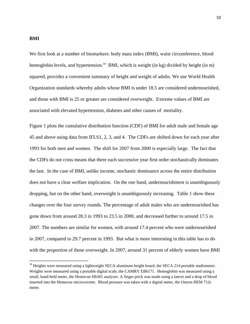
BMI

We first look at a number of biomarkers: body mass index (BMI), waist circumference, blood

hemoglobin levels, and hypertension.14 BMI, which is weight (in kg) divided by height (in m)

squared, provides a convenient summary of height and weight of adults. We use World Health

Organization standards whereby adults whose BMI is under 18.5 are considered undernourished,

and those with BMI is 25 or greater are considered overweight. Extreme values of BMI are

associated with elevated hypertension, diabetes and other causes of mortality.

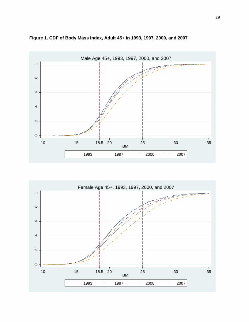
Figure 1 plots the cumulative distribution function (CDF) of BMI for adult male and female age

45 and above using data from IFLS1, 2, 3, and 4. The CDFs are shifted down for each year after

1993 for both men and women. The shift for 2007 from 2000 is especially large. The fact that

the CDFs do not cross means that there each successive year first order stochastically dominates

the last. In the case of BMI, unlike income, stochastic dominance across the entire distribution

does not have a clear welfare implication. On the one hand, undernourishment is unambiguously

dropping, but on the other hand, overweight is unambiguously increasing. Table 1 show these

changes over the four survey rounds. The percentage of adult males who are undernourished has

gone down from around 28.3 in 1993 to 23.5 in 2000, and decreased further to around 17.5 in

2007. The numbers are similar for women, with around 17.4 percent who were undernourished

in 2007, compared to 29.7 percent in 1993. But what is more interesting in this table has to do

with the proportion of those overweight. In 2007, around 31 percent of elderly women have BMI

                                                            14 Heights were measured using a lightweight SECA aluminum height board, the SECA 214 portable stadiometer. Weights were measured using a portable digital scale, the CAMRY EB6171. Hemoglobin was measured using a small, hand-held meter, the Hemocue Hb301 analyzer. A finger prick was made using a lancet and a drop of blood inserted into the Hemocue microcuvette. Blood pressure was taken with a digital meter, the Omron HEM 712c meter.

11 

 

25 or over, more than double the fraction it was in 1993. Among elderly men in 2007, 17 percent

are overweight, compared to 8.5 percent in 1993. Among the different age groups, it is the 45-54

years old that have both the lowest fraction of undernourished and the largest fraction of

overweight.

The increase over the years and the substantial degree of overweight suggests that overnutrition

and health conditions associated with it have become increasingly important in Indonesia. At the

same time, undernutrition has not entirely disappeared, though its magnitude among the aged has

sharply dropped. What is interesting, but beyond the scope of this paper is the small increase in

undernutrition between 1997 and 2000 for some age/sex groups, and the large decline in all

groups between 2000 and 2007. It could be that BMI is not increasing much or even declining

for some age/sex groups, because of adjustments in eating due to the financial crisis, whereas

economic growth was solid between 2000 and 2007, which is consistent with the large increase

of BMI during that period. The former is consistent with the findings of Thomas, Frankenberg

and Beegle, 1999, using IFLS2 and 2+.

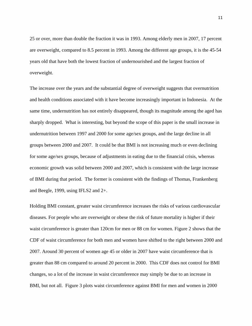
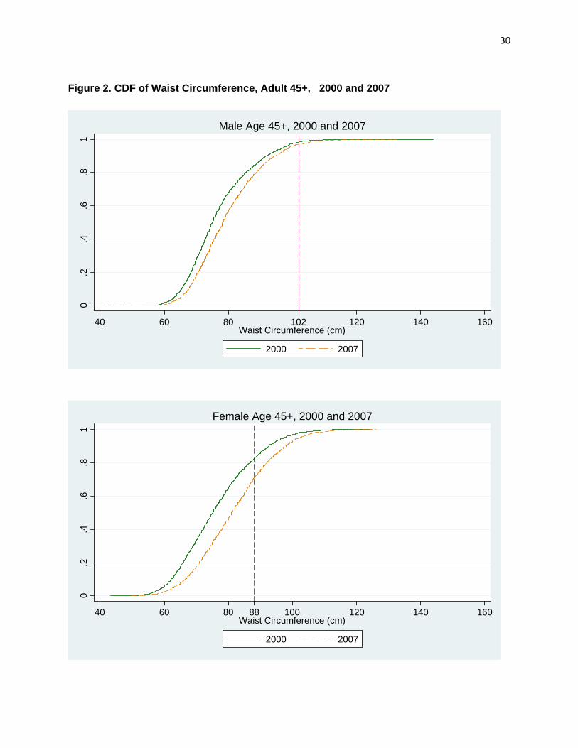
Holding BMI constant, greater waist circumference increases the risks of various cardiovascular

diseases. For people who are overweight or obese the risk of future mortality is higher if their

waist circumference is greater than 120cm for men or 88 cm for women. Figure 2 shows that the

CDF of waist circumference for both men and women have shifted to the right between 2000 and

2007. Around 30 percent of women age 45 or older in 2007 have waist circumference that is

greater than 88 cm compared to around 20 percent in 2000. This CDF does not control for BMI

changes, so a lot of the increase in waist circumference may simply be due to an increase in

BMI, but not all. Figure 3 plots waist circumference against BMI for men and women in 2000

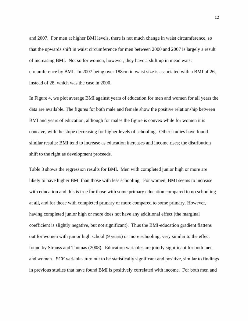
12 

 

and 2007. For men at higher BMI levels, there is not much change in waist circumference, so

that the upwards shift in waist circumference for men between 2000 and 2007 is largely a result

of increasing BMI. Not so for women, however, they have a shift up in mean waist

circumference by BMI. In 2007 being over 188cm in waist size is associated with a BMI of 26,

instead of 28, which was the case in 2000.

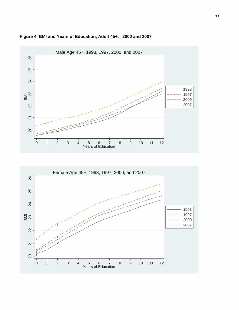
In Figure 4, we plot average BMI against years of education for men and women for all years the

data are available. The figures for both male and female show the positive relationship between

BMI and years of education, although for males the figure is convex while for women it is

concave, with the slope decreasing for higher levels of schooling. Other studies have found

similar results: BMI tend to increase as education increases and income rises; the distribution

shift to the right as development proceeds.

Table 3 shows the regression results for BMI. Men with completed junior high or more are

likely to have higher BMI than those with less schooling. For women, BMI seems to increase

with education and this is true for those with some primary education compared to no schooling

at all, and for those with completed primary or more compared to some primary. However,

having completed junior high or more does not have any additional effect (the marginal

coefficient is slightly negative, but not significant). Thus the BMI-education gradient flattens

out for women with junior high school (9 years) or more schooling; very similar to the effect

found by Strauss and Thomas (2008). Education variables are jointly significant for both men

and women. PCE variables turn out to be statistically significant and positive, similar to findings

in previous studies that have found BMI is positively correlated with income. For both men and

13 

 

women, the results show that BMI decreases at old ages. In results not shown, BMIs are also

lower for successively older birth cohorts.

One important result from this table is that the effect of education (as well as its interaction with

age in the case of men) and pce are still significant even after we control for province, province-

urban interactions, as well as province-urban-year interactions. The province-urban-year

interactions are themselves also jointly statistically significant. This is an important finding that

suggests that there is a degree of inequality of health outcomes among the elderly population

even after we control for some region characteristics, a theme that we will see again some of

other health biomarkers.

The positive interaction coefficient on the age-schooling interaction can be interpreted as

meaning that better educated men loose less BMI as they age compared to the less educated.

Since for men, more schooling, at the junior high level and above is positively correlated with

BMI, it may be that better educated men are worried about low BMI, because in the recent past

undernourishment was the bigger problem compared to overnutrition, and so try to undertake

actions to avoid that. Note that for women, the interaction is close to zero and not significant,

consistent with the flattening out of the BMI education gradient for women compared to men.

Hemoglobin

Levels of hemoglobin in blood are of interest because low levels indicate problems of anemia,

which can have various negative consequences. Iron deficiency is associated for instance with

14 

 

lower endurance for physical activity.15 For some types of employment, this deficiency may

affect productivity significantly (see Thomas et al., 2008).

Figure 5 displays the CDF of blood hemoglobin levels for elderly for 1997, 2000, and 2007

(blood hemoglobin level was not collected in 1993). The vertical lines at 13.0 dL for males and

12.0 g/dL for females in Figure 5 show the thresholds that are used in previous studies below

which work capacity is believed to be reduced.16 The figure shows the shift to the right from

previous rounds for both men and women, indicating higher levels of blood hemoglobin levels in

the population, and lower proportion of elderly below that are below the thresholds. Indeed

Table 2 shows that the proportion of elderly men with blood hemoglobin levels lower than the

threshold of 13.0 g/dL has gone down from 40.6 in 1997 to 27.12 in 2007. For women the

proportion below the threshold of 12.0 g/dL has decreased from 41.9 to 33.8.Given what we

know about what blood hemoglobin levels can tell us, this change shows an improvement in one

dimension of health in Indonesia over the years.

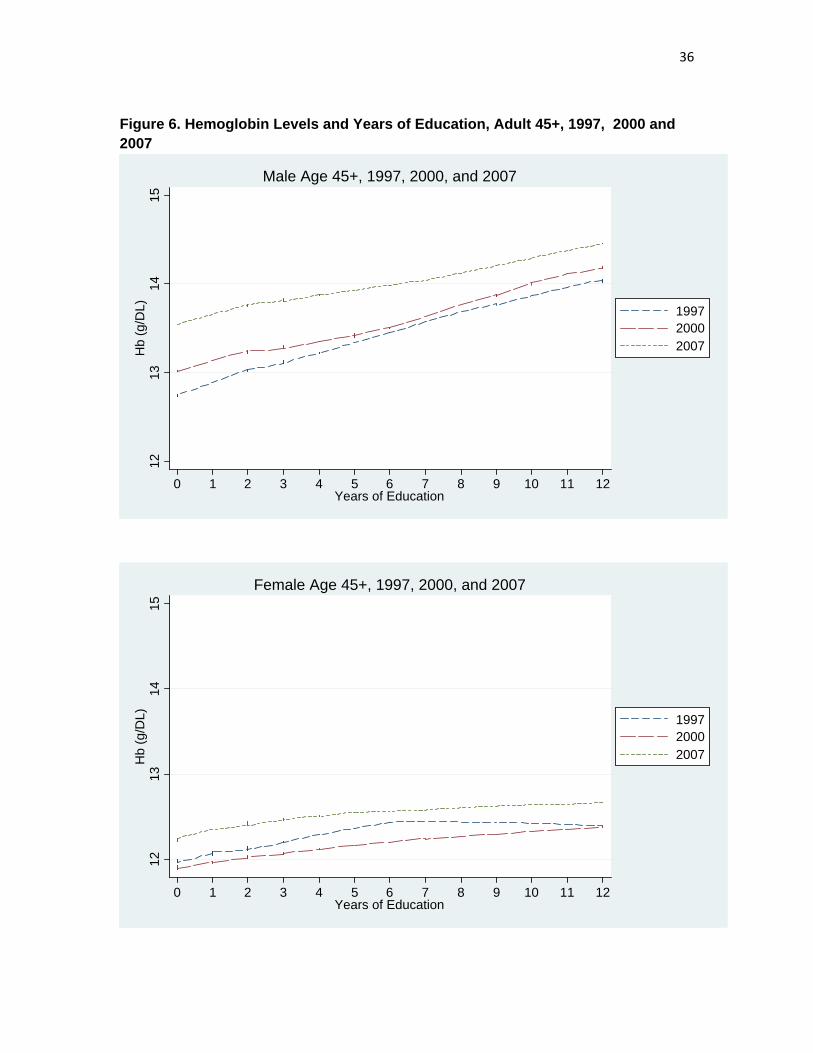
The regressions presented in Table 3 shows that older age has a strong impact on lowering blood

hemoglobin levels for both and women. There are no significant cohort effects for women,

though there are for men, with older cohorts having lower hemoglobin levels. For men, having

completed junior high school or more education is associated with higher levels of hemoglobin

compared to those with less schooling. For women having primary schooling seems to have a

                                                            15 Hemoglobin levels may also be low if a person has an infection, or for other reasons.

16 Studies have also shown that the relationship between hemoglobin level and work capacity is non-linear;higher level above the thresholds has no impact on work capacity, see for instance, Thomas et al. (2008).

15 

 

positive correlation. Log pce has a strongly positive correlation with hemoglobin at low levels

of income. Interestingly the education-age interaction has no effect.

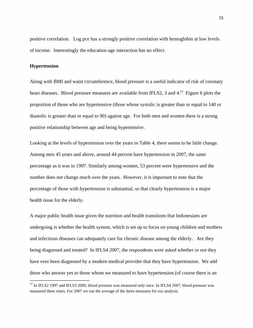
Hypertension

Along with BMI and waist circumference, blood pressure is a useful indicator of risk of coronary

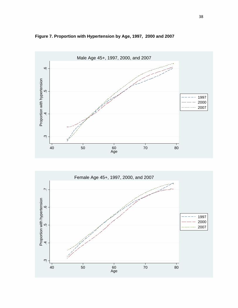
heart diseases. Blood pressure measures are available from IFLS2, 3 and 4.17 Figure 6 plots the

proportion of those who are hypertensive (those whose systolic is greater than or equal to 140 or

diastolic is greater than or equal to 90) against age. For both men and women there is a strong

positive relationship between age and being hypertensive.

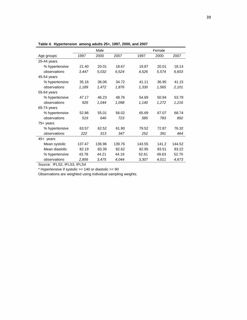
Looking at the levels of hypertension over the years in Table 4, there seems to be little change.

Among men 45 years and above, around 44 percent have hypertension in 2007, the same

percentage as it was in 1997. Similarly among women, 53 percent were hypertensive and the

number does not change much over the years. However, it is important to note that the

percentage of those with hypertension is substantial, so that clearly hypertension is a major

health issue for the elderly.

A major public health issue given the nutrition and health transitions that Indonesians are

undergoing is whether the health system, which is set up to focus on young children and mothers

and infectious diseases can adequately care for chronic disease among the elderly. Are they

being diagnosed and treated? In IFLS4 2007, the respondents were asked whether or not they

have ever been diagnosed by a modern medical provider that they have hypertension. We add

those who answer yes to those whom we measured to have hypertension (of course there is an                                                             17 In IFLS2 1997 and IFLS3 2000, blood pressure was measured only once. In IFLS4 2007, blood pressure was measured three times. For 2007 we use the average of the three measures for our analysis.

16 

 

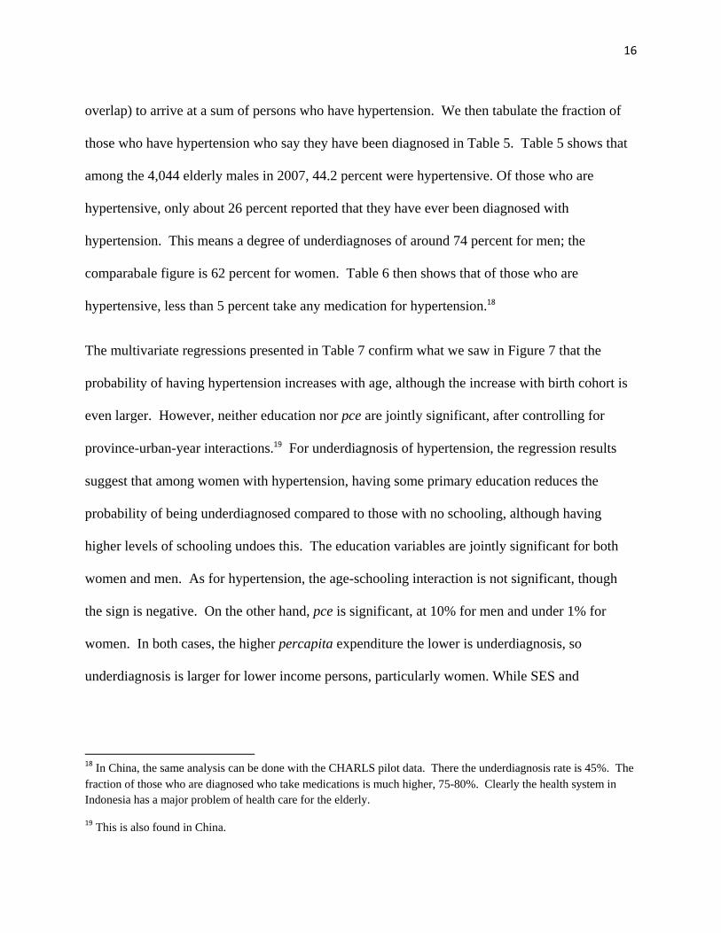
overlap) to arrive at a sum of persons who have hypertension. We then tabulate the fraction of

those who have hypertension who say they have been diagnosed in Table 5. Table 5 shows that

among the 4,044 elderly males in 2007, 44.2 percent were hypertensive. Of those who are

hypertensive, only about 26 percent reported that they have ever been diagnosed with

hypertension. This means a degree of underdiagnoses of around 74 percent for men; the

comparabale figure is 62 percent for women. Table 6 then shows that of those who are

hypertensive, less than 5 percent take any medication for hypertension.18

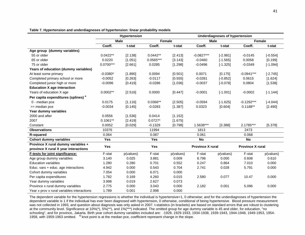
The multivariate regressions presented in Table 7 confirm what we saw in Figure 7 that the

probability of having hypertension increases with age, although the increase with birth cohort is

even larger. However, neither education nor pce are jointly significant, after controlling for

province-urban-year interactions.19 For underdiagnosis of hypertension, the regression results

suggest that among women with hypertension, having some primary education reduces the

probability of being underdiagnosed compared to those with no schooling, although having

higher levels of schooling undoes this. The education variables are jointly significant for both

women and men. As for hypertension, the age-schooling interaction is not significant, though

the sign is negative. On the other hand, pce is significant, at 10% for men and under 1% for

women. In both cases, the higher percapita expenditure the lower is underdiagnosis, so

underdiagnosis is larger for lower income persons, particularly women. While SES and

                                                            18 In China, the same analysis can be done with the CHARLS pilot data. There the underdiagnosis rate is 45%. The fraction of those who are diagnosed who take medications is much higher, 75-80%. Clearly the health system in Indonesia has a major problem of health care for the elderly.

19 This is also found in China.

17 

 

particularly pce do not have significant effect on hypertension, pce does have an effect on who

get diagnosed and presumable treated.

Cognition: word recall

Cognition has been found to be an important issue among the elderly (see McArdle, Fisher and

Kadlec, 2007). We use immediate and delayed word recall as one of the cognitive measures,

namely the episodic memory measure. In IFLS4, like HRS, respondents are read a list of ten

simple nouns and they are immediately asked to repeat as many as they can, in any order. After

answering unrelated questions on morbidity, maybe ten minutes later, the respondents are then

asked again to repeat as many words as they can. We use the average number of correctly

immediate and delayed recalled words as our memory measure (McArdle, Smith and Willis,

2009).

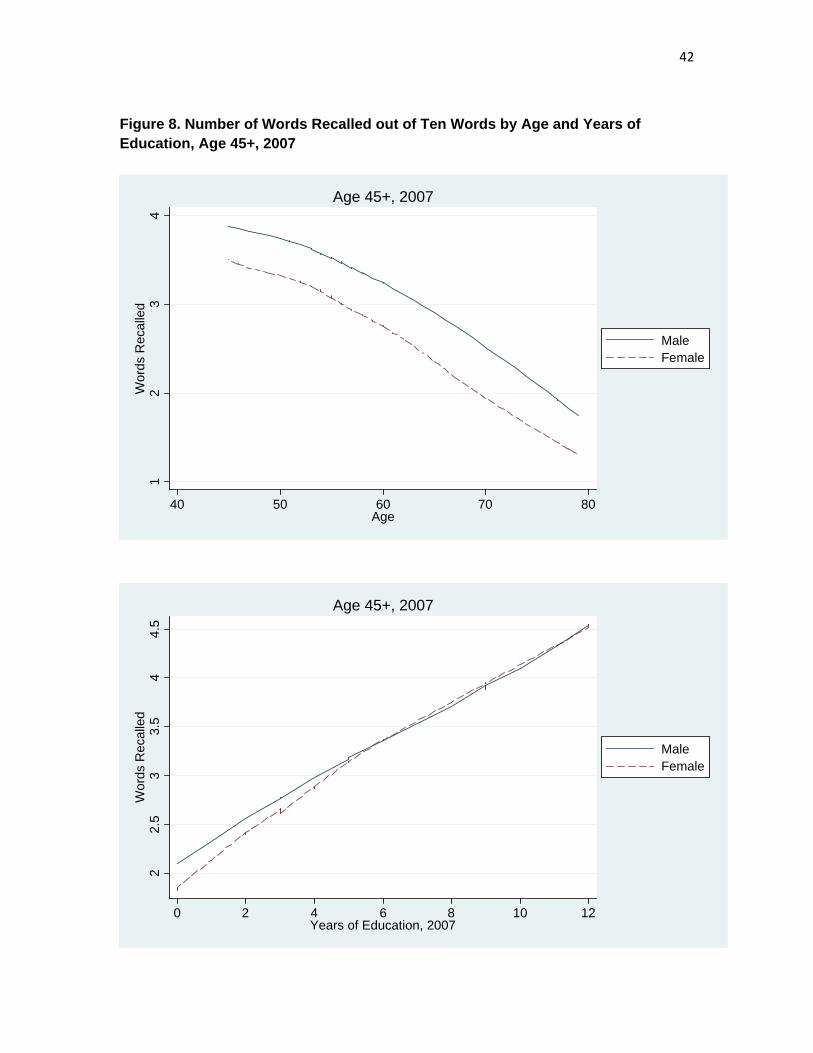
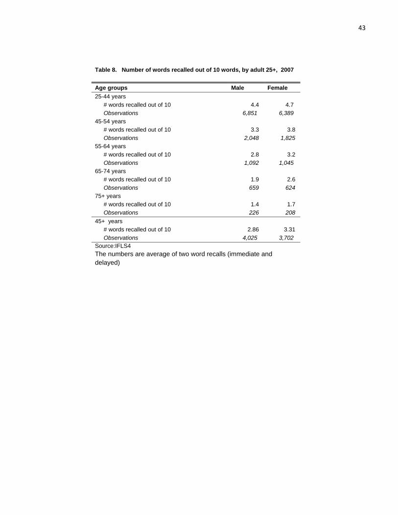
Table 8 shows the average number of words recalled by age group and sex. On average, elderly

men are able to recall 2.9 words, and elderly women are able to recall 3.2 words. Figure 8 shows

a strong negative binary relationship between the number of words recalled and age and a strong

positive relationship with years of education. Note that in the top panel, the line for men is higher

than that of women. This is partly due to the fact that at any given age, men on average are better

educated than women. Along the same lines, part of the reason that the lines coincide is that for

any given years of education, men are typically older than women. The multivariate analysis,

presented in Table 9, sheds more light on these associations.

The multivariate regression results presented in Table 9 show a strong negative relationship

between age and memory for men and women. A strong, positive relationship between

18 

 

education and memory is also evident, with strong, positive coefficients on the age-schooling

interaction terms, suggesting that education counters the negative effects of aging on memory.

The pce variables are jointly significant, positively correlated with word recall.

Self-reported measurements: ADL, IADL, mental health, and general health status

Physical functioning assessment, ADLs, and IADLs

The self-assessment of basic physical functioning and activities of daily living (ADLs) provide

useful information about a person’s functional status and have been shown to be correlated with

SES measures (see for instance, Strauss et al., 1993).20 We plot the average number of ADLs

that an elderly had difficulties with against age and education in Figures 9 and 10. The figures

show that the number of ADLs a person had difficulties with rises with age for both men and

women, although for women the relationship seems to be stronger. In contrast there does not

seem to be a strong binary relationship between education and the number of ADLs with

difficulty. Table 10 shows that the proportion of elderly with any difficulty with physical

functioning/ADL did not change much between 1997, 2000, and 2007.

In addition to ADLs, in 2007 the survey also collects self-assessed information about

instrumental activities of daily living (IADL), which includes activities not necessary for

fundamental functioning, but required to be able to live independently. Activities included are:

to shop for personal needs, to prepare one’s own meal, to take a medicine, to visit a neighbor,

and to travel. Similar to ADL, for IADL we also see that the number of difficulties increase with                                                             20 Our physical activities and ADL assessments include: carrying a heavy load for 20 meters, walking for 5 kilometers, to bow, squat, or kneel, sweeping the house floor yard, to draw a pail of water from a well, to stand from sitting from the floor without help, to stand from sitting position without help, to go the bathroom without help, and to dress without help.

19 

 

age and the number is higher for women than men (Figure 11). Education seems to be

negatively associated with IADL if only slightly.

The regressions reported in Table 12 confirm the positive association between the number of

ADLs or IADLs a person had difficulty with and age. For difficulty with IADLs there are

significant negative interactions between years of schooling and age. Apparently schooling does

help to mitigate the impact of aging on having difficulties with IADLs, for both men and women.

PCE seems to be negatively correlated with both ADLs and IADLs, but more important for men.

CES-D 10 score

As a measure of mental health the respondents were administered self-reported depression scale

from the short version of the CES-D Scale, one of the major international scales of depression

used in general populations. Higher scores on the CES-D scale indicates a higher likelihood of

having major depression .21 Some recent studies have failed to find a relationship between

depression and education or income (see Das, Do, Friedman, McKenzie and Scott, 2007, for

example), however other studies have found such correlations (Patel and Kleinman, 2003, survey

several studies that do find negative correlations between depression and SES). For Indonesia,

Friedman and Thomas (2008) find that the economic crisis fueled depression indicators,

especially for the more vulnerable population.22

                                                            21 The answers for CES-D are on a four-scale metric, from rarely, to some days (1-2 days), to occasionally (3-4 days) to most of the time (5-7 days). We score these answers in the way suggested by the Stanford group that created the CES-D, using numbers from 0 for rarely to 3 for most of the time, for negative questions such as do you feel sad. For positive questions do you feel happy, the scoring is reversed from 0 for most of the time to 3 for rarely.

22 They also use IFLS data, from 1993 and 2000. Unfortunately the depression scale that IFLS had been using was not as widely used as the CES-D scale and so we switched scales in 2007 to be more comparable to other

20 

 

Figure 12 displays the relationship between CES-D scores and age (top panel) and with years of

education (bottom). For both elderly men and elderly women, CES-D scores increase with age,

and decrease with years of education. On average women have higher CES-D scores than men.

The mean CES-D scores among 45 years old and older are 3.3 for men and 3.8 for women.

The regressions using CES-D as dependent variable show that the education variables are not

jointly statistically significant by themselves, but are highly negatively so for both men and

women when interacted with age. So again, schooling seems to mitigate the aging process. On

the other hand, the expenditure variables are not significant. So our results do support previous

studies that show negative correlations between schooling and depression, though not with pce.23

General Health Status

In all four waves of the survey, respondents were asked to assess their own health status. They

were asked to answer the question “In general how is your health” with the following options:

very healthy, somewhat healthy, somewhat unhealthy, and unhealthy. We code those who

answered “somewhat unhealthy” and “unhealthy” as reporting to have “poor health”. General

health status is very widely used as a health indicator. There is a worry that how one reports

their health may be affected with how often they see doctors, or other, more general views of the

world (Strauss and Thomas, 1995, 1998), but it is the case that perceptions of general health do

predict subsequent mortality in surveys such as the HRS and ELSA (for example, Banks et al.,

2009).

                                                                                                                                                                                                international surveys, especially the HRS-type surveys. This means that in this paper we can only use the CES-D scale for one year, 2007.

23 Similar results are again found in the CHARLS data for China.

21 

 

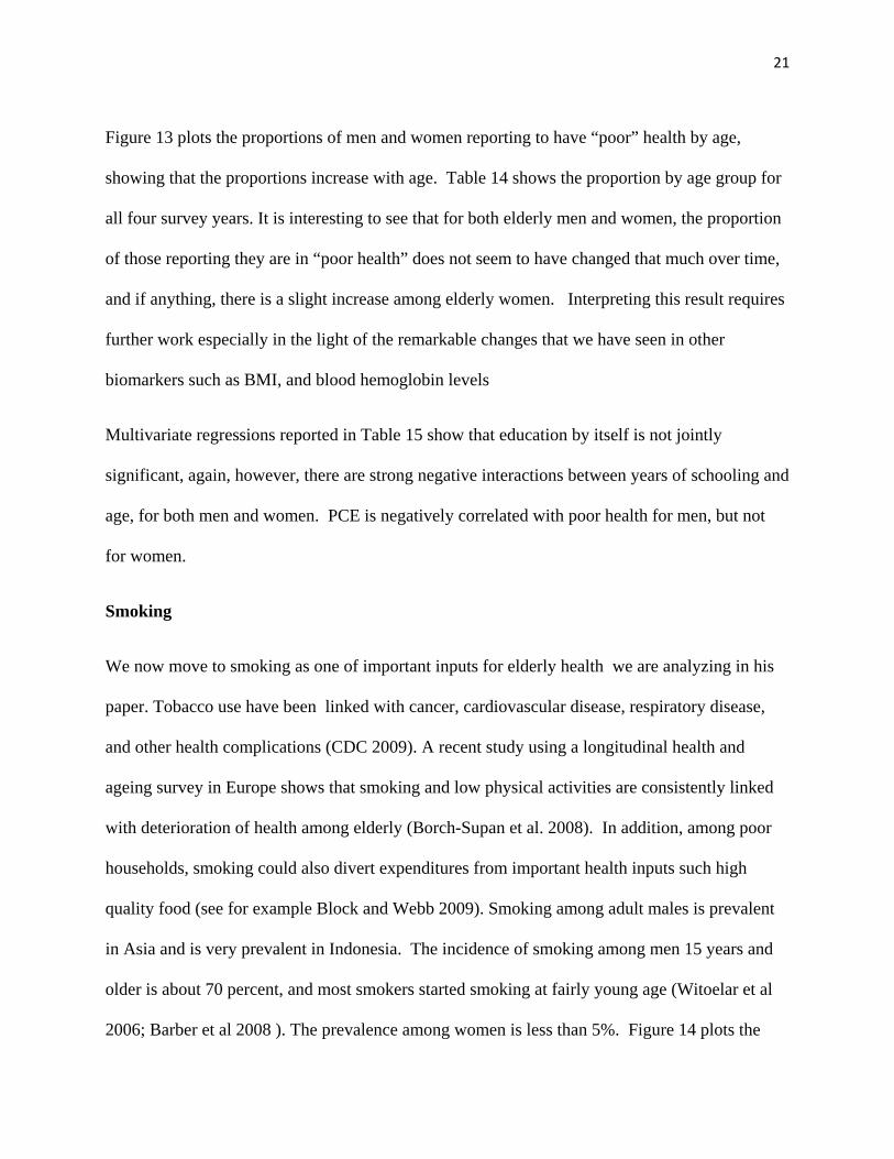
Figure 13 plots the proportions of men and women reporting to have “poor” health by age,

showing that the proportions increase with age. Table 14 shows the proportion by age group for

all four survey years. It is interesting to see that for both elderly men and women, the proportion

of those reporting they are in “poor health” does not seem to have changed that much over time,

and if anything, there is a slight increase among elderly women. Interpreting this result requires

further work especially in the light of the remarkable changes that we have seen in other

biomarkers such as BMI, and blood hemoglobin levels

Multivariate regressions reported in Table 15 show that education by itself is not jointly

significant, again, however, there are strong negative interactions between years of schooling and

age, for both men and women. PCE is negatively correlated with poor health for men, but not

for women.

Smoking

We now move to smoking as one of important inputs for elderly health we are analyzing in his

paper. Tobacco use have been linked with cancer, cardiovascular disease, respiratory disease,

and other health complications (CDC 2009). A recent study using a longitudinal health and

ageing survey in Europe shows that smoking and low physical activities are consistently linked

with deterioration of health among elderly (Borch-Supan et al. 2008). In addition, among poor

households, smoking could also divert expenditures from important health inputs such high

quality food (see for example Block and Webb 2009). Smoking among adult males is prevalent

in Asia and is very prevalent in Indonesia. The incidence of smoking among men 15 years and

older is about 70 percent, and most smokers started smoking at fairly young age (Witoelar et al

2006; Barber et al 2008 ). The prevalence among women is less than 5%. Figure 14 plots the

22 

 

proportion of elderly men who currently smoking in each survey year against age. The figure

shows that the incidence decreases with age.

Table 15 shows that indeed the proportion currently smoking decreases with age and this is true

for every survey year. The table also shows the proportion of individuals who have ever smoked.

The numbers suggest that most who ever smoked do not quit especially when they are relatively

younger. But even among the 65 and over, of those 80 percent who have ever smoked, more than

60 percent do not quit.

The multivariate regression results indicate that incidence of smoking decreases with age (there

are no significant cohort effects), and increases with education. However, there exists a

significant negative interaction between age and schooling, so that higher schooling apparently is

correlated with a stronger decline of smoking with age. PCE variables suggest that increases in

income for higher income households, reduces the likelihood of currently smoking .

Physical activities

Lastly, we look at time spent on physical activities, which is based on new questions added in

IFLS4 2007. The questions asked whether and how much time respondents engaged in vigorous

and moderate physical activities, walking, and sitting in the past week. We focus on vigorous and

moderate physical activities.24 Other studies have suggested that time spent on energy-intensive

                                                            24 The question for vigorous physical activities is: “Now, think about all the vigorous activities which take hard physical effort that you did in the last 7 days. Vigorous activities make you breathe much harder than normal and may include heavy lifting, digging, plowing, aerobics, fast bicycling, cycling with loads. Think only about those physical activities that you did for at least 10 minutes at a time”. The question for moderate physical activities is: “Now think about activities which take moderate physical effort that you did in the last 7 days. Moderate physical activities make you breathe somewhat harder than normal and may include carrying light loads, bicycling at a regular pace, or mopping the floor. Again, think about only those physical activitiesthat you did for at least 10 minutes at a time.”

23 

 

activities may be able to explain the rising rate of obesity (Cutler and Glaeser, 2003) and explain

cross-country differences in obesity among older Americans and Europeans (Michaud, van

Soest, Andreyeva 2007). Low physical activities is linked to deterioration of health among

elderly in Europe (Borch-Supan et al 2008).

Figure 15 shows that the proportion of 45 and older men who carry out vigorous physical

activities to be much higher than women and it is decreasing with years of education. The

proportion of men and women who do moderate physical activities are more similar. Table 18

shows that around 48 percent of men 45 and above reported to have been engaged in vigorous

activities compared to 18 percent of women.

Regressions show that the likelihood of engaging in vigorous physical activities get smaller as

one gets older. For men, the education variables are jointly significant. Men with some primary

school education but who did not complete junior high school are more likely to carry out

vigorous physical activities than either those who have no schooling, but the marginal schooling

effects at higher levels are negative. As men age, the decline in vigorous activities is stronger if

they have higher schooling. Men with higher income are also less likely to engage in vigorous

physical activities. For women engaging in moderate activities, more education has a positive

impact, which is reduced with greater age.

4. Conclusions

Indonesia has undergone major changes in multiple dimensions since the Indonesia Family Life

Survey (IFLS) was first fielded in 1993. Among these changes has been moving along the health

and nutrition transition. IFLS is very well-suited to examine those changes.

24 

 

Overall there have been significant changes in health outcomes among elderly Indonesians over

the 15 year period of the IFLS. Much of the change can be seen as improvements such as the

movement out of undernutrition and communicable disease as well as the increasing levels of

hemoglobin. On the other hand, other changes such as the increase in overweight and waist

circumference, especially among women, and continuing high levels of hypertension that seems

to be inadequately addressed by the health system, indicate that the elderly population in

Indonesia is increasingly exposed to higher risk factors that are correlated with chronic problems

such as cardiovascular diseases and diabetes.

And yet with these changes, other health risk factors have shown little change over this fifteen

year period, including prevalence of hypertension, the number of ADLs that respondents say

they have difficulty in performing and a measure of self-reported general health. This is quite

interesting because this period has seen major gyrations in economic activity, including strong

growth from 1993 to 1996, a major economic collapse from late 1997 to 1998 and a strong

recovery from 2000 to 2007. The financial crisis may have slowed the nutrition transition, and

some of our evidence is consistent with that conjecture. Overall, apart from the health and

nutrition transitions, it is not apparent from this evidence that some parts of health, especially

self-assessed measures, have changed much with the strong economic movements over this time

frame. Yet other measures, especially nutrition-based measures do seem to have evolved.

The relationship between health and SES at different stages in the life cycle is always difficult to

disentangle. IFLS enables us to provide some important findings that contribute to our

understanding of the relationships.

25 

 

In this paper we examine correlations between SES and many health outcomes and behaviors for

the elderly. Past work has usually been limited to just a small number of health outcomes and

has not usually examined the elderly. To the extent that controlling for time, community, and

their interactions account for differences in prices, health care availability and quality in the

communities over time, the significant correlations that still exist between SES and many of the

health outcomes indicate that there is a substantial degree of inequality of health among the

elderly population. Furthermore, the positive correlations that we find between SES and most of

the good health outcomes, and the fact that education tends to suppress the negative impacts of

age on many health outcomes suggests that part of the correlations is causal, running from SES

to health. These findings are indicative of some pathways through which health outcomes could

be affected by changes in policy or external shocks that influence SES. Investigating these

pathways further is a challenge for future research.

26 

 

References

Banks, James, Alastair Muriel and James P. Smith, 2009. “Disease prevalence, incidence and determinants of mortality in the United States and England”, manuscript, Department of Economics, University College London.

Barber, Sarah, Sri Moertiningsih Aditomo, Abdillah Ahsan, Dianhadi Setyonaluri, 2008. Tobacco Economics in Indonesia. Paris: International Union Against Tuberculosis and Lung Disease.

Barker, David, 1994. Mothers, babies and health in later life, London: BMJ Publishing Group.

Barrera, Albino, 1990. “The role of mother’s schooling and its interaction with public health programs in child health production”, Journal of Development Economics, 32(1):69-92.

Block, Steven, and Patrick Webb, 2009. “Up in Smoke: Tobacco Use, Expenditure on Food, and Child Malnutrition in Developing Countries” Economic Development and Cultural Chang, 58 (October 2009) 1-23.

Börch-Supan, Axel, Agar Brugiavini, Hendrik Jürges, Arie Kapteyn, Johan Mackenbach, Johannes Siegrist, Guglielmo Webger, 2008. First Results from the Survey of Health, Ageing and Retirement in Europe (2004-2007). Mannheim Research Institute for the Economics of the Aging (MEA).

CDC (Centers for Disease Control and Prevention). 2009. “Health Effects of Cigarette Smoking.”http://www.cdc.gov/tobacco/data_statistics/fact_sheets/health_effects/effects_cig_smoking/.

Cutler, David M., Edward Glaeser, and Jesse M. Shapiro, 2003. “Why Have Americans Become More Obese?” Journal of Economic Perspective. 17(3): 93-118.

Das, Jishnu, Quy-Toan, Do, Jed Friedman, David McKenzie, and Kinnon Scott, 2007. “Mental health and poverty in developing countries”, Social Science and Medicine, 65(3):467-480.

Friedman, Jed and Duncan Thomas, 2008. “Psychological health, before, during and after an economic crisis: Results from Indonesia 1993-2000”, World Bank Economic Review, 23(1):57-76.

Gluckman, Peter and Mark Hanson, 2005. The fetal matrix: Evolution, development and disease, Cambridge: Cambridge University Press.

Indonesian Public Health Association. 1993. “Analysis of the Health Transition in Indonesia: Implications for Health Policy.” Jakarta, Indonesia: Indonesian Public Health Association.

Kinsella, Kevin and Wan He, 2009. An aging world: 2008, US Census Bureau, International Population Reports, PS95/09-1, Washington D.C.: US Government Printing Office.

27 

 

McArdle, John, Gwenith Fisher and Kelly Kadlec, 2007. “Latent variable analysis of age trends in tests of cognitive ability in the Health and Retirement Survey, 1992-2004”, Psychology and Aging, 22(3):525-545.

McArdle, John, James P. Smith and Robert Willis, 2009. “Cognition and economic outcomes in the Health and Retirement Survey”, manuscript, RAND Corporation, Santa Monica, CA.

Michaud, Pierre-Carl, Arthur H.O. van Soest, and Tatiana Andreyeva, 2007. “Cross Country Variation in Obesity Patterns among Older Americans and Europeans”. Forum for Health Economics and Policy, 10(2):

Monteiro, Carlos, Erly Moura, Wolney Conde, and Barry Popkin, 2004. “Socioeconomic status and obesity in adult populations of developing countries”, Bulletin of the World Health Organization, 82(12):940-946.

Patel, V. and A. Kleinman, 2003. “Poverty and common mental disorders in developing countries”, Bulletin of the World Health Organization, 81(8):609-615.

Popkin, Barry, 1994. “The nutrition transition in low-income countries: An emerging crisis”, Nutrition Reviews, 52(9):285-298.

Strauss, John, Paul Gertler, Omar Rahman and Kristen Fox, 1993. “Gender and life-cycle differentials in the patterns and determinants of adult health”, Journal of Human Resources, 28(4):791-837.

Strauss, John and Duncan Thomas, 1995. “Human resources: empirical modeling of household and family decisions”, in J.R. Behrman and T.N. Srinivasan (eds.), Handbook of Development Economics, Volume 3A, Amsterdam: North Holland Press.

Strauss, John and Duncan Thomas, 1998. “Health, nutrition and economic development”, Journal of Economic Literature, 36(3):766-817.

Strauss, John, Kathleen Beegle, Agus Dwiyanto, Yulia Herawati, Daan Pattinasarany, Elan Satriawan, Bondan Sikoki, Sukamdi and Firman Witoelar, 2004. Indonesian Living Standards Before and After the Financial Crisis, Singapore: Institute for Southeast Asian Studies.

Strauss, John and Duncan Thomas. 2008. “Health over the life course”, in T.P. Schultz and J. Strauss (eds.), Handbook of Development Economics, Volume 4, Amsterdam: North Holland Press.

Strauss, John, Firman Witoelar, Bondan Sikoki and Anna Marie Wattie, 2009. “The fourth wave of the Indonesia Family Life Survey: Overview and field report, Volume 1”, Working Paper WR-675/1-NIA/NICHD, Labor and Population Program, RAND Corporation, Santa Monica, CA.

Thomas, Duncan, John Strauss and Maria-Helena Henriques, 1990. “Child survival, height for age and household characteristics in Brazil”, Journal of Development Economics, 33(2):197-234.

28 

 

Thomas, Duncan, Elizabeth Frankenberg and Kathleen Beegle, 1999. “The real costs of Indonesia’s economic crisis, Labor and Population Working Paper No. 99-04, RAND Corporation, Santa Monica CA.

Thomas, Duncan, Elizabeth Frankenberg, Jed Friedman, Jean-Pierre Habicht, Mohammed Hakimi, Nicholas Ingwersen, Jaswadi, Nathan Jones, Christopher McKelvey, Gretel Pelto, Bondan Sikoki, Teresa Seeman, James P. Smith, Cecep Sumantri, Wayan Suriastini and Siswanto Wilopo, 2008. “Causal effect of health on social and economic prosperity: Experimental evidence”, manuscript, Department of Economics, Duke University.

Witoelar, Firman, John Strauss, Pungpond Rukumnuaykit, (2006). “Smoking behavior among youth in a developing country:The case of Indonesia”. Mimeo, University of Southern California.

29 

 

Figure 1. CDF of Body Mass Index, Adult 45+ in 1993, 1997, 2000, and 2007

 

0.2

.4.6

.81

10 15 18.5 20 25 30 35BMI

1993 1997 2000 2007

Male Age 45+, 1993, 1997, 2000, and 2007

   

0.2

.4.6

.81

10 15 18.5 20 25 30 35BMI

1993 1997 2000 2007

Female Age 45+, 1993, 1997, 2000, and 2007

 

30 

 

Figure 2. CDF of Waist Circumference, Adult 45+, 2000 and 2007  

0.2

.4.6

.81

40 60 80 102 120 140 160Waist Circumference (cm)

2000 2007

Male Age 45+, 2000 and 2007

   

0.2

.4.6

.81

40 60 80 100 120 140 16088Waist Circumference (cm)

2000 2007

Female Age 45+, 2000 and 2007

 

31 

 

Figure 3. Waist Circumference against BMI: Adult 45+, 2000 and 2007 50

6070

8090

100

110

120

Wai

st (c

m)

12 14 16 18 20 22 24 26 28 30 32 34 36BMI

20002007

Male 45+

 

 

5060

7080

9010

011

012

0W

aist

(cm

)

12 14 16 18 20 22 24 26 28 30 32 34 36BMI

20002007

Female 45+

32 

 

 Table 1. Percentage of Adults 25+ Undernourished or Overweight, 1993 1997, 2000, and 2007

Men Women Age groups 1993 1997 2000 2007 1993 1997 2000 2007 25-44 years % Undernourished (BMI <18.5) 10.94 12.61 13.81 11.58 12.15 10.46 10.25 7.88 % Overweight ( BMI >=25.0) 9.53 10.91 12.81 19.15 19.64 22.24 25.44 35.05 Observations 2,825 3,444 5,006 6,492 3,608 4,558 5,601 6,914 45-54 years % Undernourished (BMI <18.5) 17.02 16.34 12.49 9.46 22.28 16.52 12.98 9.39 % Overweight ( BMI >=25.0) 11.25 13.32 17.00 22.65 17.04 24.46 30.83 40.18 Observations 1,042 1,187 1,467 1,870 1,232 1,333 1,561 2,106 55-64 years % Undernourished (BMI <18.5) 29.88 27.07 24.22 18.22 31.96 28.15 27.14 16.64 % Overweight ( BMI >=25.0) 8.11 9.06 12.68 17.26 14.24 17.82 21.19 30.57 Observations 819 923 1,035 1,096 942 1,132 1,261 1,211 65-74 years % Undernourished (BMI <18.5) 42.50 39.46 35.66 27.95 36.86 33.89 34.26 29.57 % Overweight ( BMI >=25.0) 4.65 6.28 7.37 8.59 10.70 12.29 15.44 18.82 Observations 481 512 639 713 485 581 763 878 75+ years % Undernourished (BMI <18.5) 48.68 50.36 48.39 38.05 50.09 46.35 44.65 33.60 % Overweight ( BMI >=25.0) 4.33 2.49 3.05 6.31 4.25 8.30 8.98 13.96 Observations 172 218 306 338 184 241 359 438 45+ years Mean BMI 20.30 20.69 21.06 21.75 20.86 21.43 21.88 22.90 % Undernourished (<18.5) 28.25 26.60 23.50 17.54 29.77 25.78 24.51 17.40 % Overweight ( BMI >=25.0) 8.49 9.83 12.68 17.31 14.20 18.84 22.78 31.14 Observations 2,514 2,840 3,447 4,017 2,843 3,287 3,944 4,633 Source: IFLS1, IFLS2, IFLS3, and IFLS4 Observations are weighted using individual sampling weights.

33 

 

Figure 4. BMI and Years of Education, Adult 45+, 2000 and 2007  

2021

2223

2425

26BM

I

0 1 2 3 4 5 6 7 8 9 10 11 12Years of Education

1993199720002007

Male Age 45+, 1993, 1997, 2000, and 2007

   

2021

2223

2425

26BM

I

0 1 2 3 4 5 6 7 8 9 10 11 12Years of Education

1993199720002007

Female Age 45+, 1993, 1997, 2000, and 2007

 

34 

 

Figure 5. CDF of Hemoglobin Levels, Adult 45+, 1997, 2000 and 2007  

0.2

.4.6

.81

8 9 10 11 12 13 14 15 16 17Hb level

1997 2000 2007

Male Age 45+,1997, 2000, and 2007

   

0.2

.4.6

.81

8 9 10 11 12 13 14 15 16 17Hb level

1997 2000 2007

Female Age 45+, 1997, 2000, and 2007

35 

 

Table 2. Percentage of adults 25+ with blood hemoglobin level below 13.0 g/dL (men) or 12.0 g/dL (women), 1997, 2000 and 2007

Men Women Age groups 1997 2000 2007 1997 2000 2007 25-44 years % <12.0/13.0 22.01 15.45 9.69 36.07 38.62 26.58 Observations 3,397 4,961 6,485 4,478 5,555 6,904 45-54 years % <12.0/13.0 32.22 22.09 17.72 39.49 39.96 28.08 Observations 1,167 1,460 1,869 1,298 1,553 2,091 55-64 years % <12.0/13.0 41.57 37.32 26.01 40.16 41.96 32.82 Observations 911 1,039 1,093 1,122 1,260 1,212 65-74 years % <12.0/13.0 48.53 46.58 40.86 46.00 48.93 40.25 Observations 513 645 728 575 774 886 75+ years % <12.0/13.0 62.81 53.60 52.24 53.52 53.49 50.06 Observations 220 312 350 237 387 461 45+ years Mean HB level 13.29 13.51 13.99 12.10 12.03 12.42 %<12.0/13.0 40.62 34.08 27.12 41.91 43.66 33.81 Observations 2,811 3,456 4,040 3,232 3,974 4,650 Source: IFLS2, IFLS3, IFLS4 Observations are weighted using individual sampling weights. The thresholds are12.0 g/dL for women and 13.0 g/dL for men.

36 

 

Figure 6. Hemoglobin Levels and Years of Education, Adult 45+, 1997, 2000 and 2007

1213

1415

Hb

(g/D

L)

0 1 2 3 4 5 6 7 8 9 10 11 12Years of Education

199720002007

Male Age 45+, 1997, 2000, and 2007

   

1213

1415

Hb

(g/D

L)

0 1 2 3 4 5 6 7 8 9 10 11 12Years of Education

199720002007

Female Age 45+, 1997, 2000, and 2007

  

37 

 

Table 3. Multivariate regressions: BMI and Hemoglobin Levels BMI Hemoglobin Male Female Male Female Coeff. t-stat Coeff. t-stat Coeff. t-stat Coeff. t-stat Age group (dummy variables) 55 or older -0.0611 [0.594] 0.1519 [1.288] -0.2755*** [2.790] -0.0242 [0.435] 65 or older -0.3300*** [2.919] -0.0377 [0.273] -0.2461*** [2.640] -0.1390* [1.687] 75 or older -0.4208*** [2.926] -0.6792*** [4.120] -0.3387*** [2.810] -0.2965*** [3.636] Years of education (dummy variables) At least some primary -0.1288 [1.013] 0.5536*** [3.048] 0.0837 [0.963] 0.0710 [1.104] Completed primary school or more -0.0063 [0.049] 0.3883** [2.002] -0.0125 [0.159] 0.0665 [1.001] Completed junior high or more 0.5712*** [3.172] -0.1946 [0.753] 0.2193** [2.410] -0.1317 [1.522] Education X age interaction Years of education X age 0.0018*** [3.817] 0.0012* [1.707] 0.0001 [0.594] 0.0003 [1.285] Per capita expenditures (splines) a 0 - median pce 0.6927*** [7.844] 0.8041*** [7.001] 0.2713*** [4.413] 0.1223** [2.376] >= median pce 0.0416 [0.285] 0.0210 [0.126] -0.0655 [0.753] -0.0608 [0.820] Year dummy variables 1997 and after -0.5370** [2.267] -0.0833 [0.271] 2000 and after -0.1500 [0.708] -0.4314* [1.681] 0.2679** [2.199] 0.1645 [1.002] 2007 -0.3336 [1.030] -0.3490 [1.214] -0.4882*** [3.013] 0.0879 [0.571] Constant 14.8422*** [15.400] 15.7249*** [12.237] 10.9485*** [15.709] 10.5401*** [18.070] Observations 12836 14735 10305 11853 R-squared 0.228 0.222 0.123 0.056 Cohort dummy variables Yes Yes Yes Yes Province X rural dummy variables + province X rural X year interactions Yes

Yes

Yes

Yes

F-tests for joint significance: F-stat p(values) F-stat p(values) F-stat p(values) F-stat p(values) Age group dummy variables 5.796 0.001 7.817 0.000 4.031 0.008 5.412 0.001 Education variables 6.194 0.000 6.245 0.000 2.083 0.102 2.099 0.099 Educ. vars + educ. age interactions 40.29 0.000 22.00 0.000 8.541 0.000 5.151 0.000 Cohort dummy variables 8.822 0.000 13.89 0.000 2.294 0.026 1.308 0.245 Per capita expenditures 79.31 0.000 75.89 0.000 30.93 0.000 5.960 0.003 Year dummy variables 3.073 0.028 1.631 0.181 5.171 0.006 1.000 0.369 Province x rural dummy variables 4.653 0.000 6.799 0.000 5.139 0.000 3.779 0.000 Year x prov x rural variables interactions 2.090 0.000 2.790 0.000 4.199 0.000 2.523 0.000

The dependent variable for BMI regressions is the BMI for hemoglobin the hemoglobin level (g/dL). Blood hemoglobin level was not collected in 1993. t-statistics (in brackets) are based on standard errors that are robust to clustering at the community level. * significant at 10%; ** significant at 5%; *** significant at 1%. The omitted group for age dummy variable is 45 and older, for education, "no schooling", and for province, Jakarta. Birth year cohort dummy variables included are: -1928, 1929-1933, 1934-1938, 1939-1943, 1944-1948, 1949-1953, 1954-1958, with 1959-1963 omitted. a) knot point is at the median pce, coefficient represent change in the slope.

38 

 

Figure 7. Proportion with Hypertension by Age, 1997, 2000 and 2007   

.3.4

.5.6

Prop

ortio

n w

ith h

yper

tens

ion

40 50 60 70 80Age

199720002007

Male Age 45+, 1997, 2000, and 2007

   

.3.4

.5.6

.7Pr

opor

tion

with

hyp

erte

nsio

n

40 50 60 70 80Age

199720002007

Female Age 45+, 1997, 2000, and 2007

39 

 

 Table 4. Hypertension among adults 25+, 1997, 2000, and 2007

Male Female Age groups 1997 2000 2007 1997 2000 2007 25-44 years % hypertensive 21.40 20.01 18.67 19.87 20.01 18.14 observations 3,447 5,032 6,524 4,526 5,574 6,603 45-54 years % hypertensive 35.16 36.06 34.72 41.11 36.95 41.15 observations 1,189 1,472 1,876 1,330 1,565 2,101 55-64 years % hypertensive 47.17 46.23 48.76 54.69 50.94 53.79 observations 926 1,044 1,098 1,140 1,272 1,216 65-74 years % hypertensive 52.86 55.01 56.02 65.69 67.07 68.74 observations 519 646 723 585 783 892 75+ years % hypertensive 63.57 62.52 61.90 79.52 72.87 76.32 observations 222 313 347 252 391 464 45+ years Mean systolic 137.47 136.96 139.76 143.55 141.2 144.52 Mean diastolic 82.19 83.39 82.62 82.95 83.51 83.22 % hypertensive 43.78 44.21 44.19 52.61 49.63 52.70 observations 2,856 3,475 4,044 3,307 4,011 4,673 Source: IFLS2, IFLS3, IFLS4 * Hypertensive if systolic >= 140 or diastolic >= 90 Observations are weighted using individual sampling weights.

40 

 

 Table 5. Underdiagnosis of hypertension, adult 45+, 2007 Adult 45 + years Men Women Observations 4,044 4,676 % hypertensive 44.2 52.8 % diagnosed a) 26.4 37.9 Underdiagnosis of hypertension by education, adult 45+ highest completed level of education % underdiagnosed a) no schooling 79.0 69.4 primary schooling 74.4 58.1 junior high 73.2 52.1 senior high + 68.0 62.3 all adult 45+ 73.6 62.1

Source: IFLS4 Observations are weighted using individual sampling weights. a) "Diagnosed" if answered "Yes" to the question "Has a doctor/nurse/paramedic ever told you that you have hypertension?". Percentages are out of individuals 45+ whose systolic>=140 or diastolic >=90.

   Table 6. Hypertension and medication, adult 45+, 2000 and 2007

Adult 45 + years Men Women 2000 2007 2000 2007

Observations

3,477

4,044

3,631

4,674 % hypertensive 44.2 44.2 49.6 52.8 % taking medication for hypertension a) 2.6 4.7 2.5 4.7 a) Percentages are out of individuals 45+ whose systolic >=140 or diastolic >=90 Hypertensive and not taking medication, by completed education a)

Men Women Highest completed level of education 2000 2007 2000 2007 no schooling 98.7 97.6 98.7 97.3 primary schooling 99.1 96.7 96.9 94.9 junior high 95.4 91.2 96.7 88.1 senior high + 93.9 92.5 92.3 94.1 all adult 45+ 97.4 95.3 97.5 95.4 Source: IFLS3 and IFLS4 a) Percentages are out of individuals 45+ whose systolic >=140 or diastolic >=90. Observations are weighted using individual sampling weights.

41 

 

Table 7. Hypertension and underdiagnoses of hypertension: linear probability models Hypertension Underdiagnoses of hypertension Male Female Male Female Coeff. t-stat Coeff. t-stat Coeff. t-stat Coeff. t-stat Age group (dummy variables) 55 or older 0.0422** [2.138] 0.0442** [2.413] -0.0827*** [-2.981] -0.0145 [-0.554] 65 or older 0.0220 [1.051] 0.0565*** [3.143] -0.0460 [-1.565] 0.0058 [0.199] 75 or older 0.0700*** [2.661] 0.0285 [1.298] -0.0496 [-1.325] -0.0349 [-1.094] Years of education (dummy variables) At least some primary -0.0380* [1.890] 0.0094 [0.501] 0.0071 [0.175] -0.0941*** [-2.745] Completed primary school or more -0.0052 [0.263] -0.0117 [0.555] -0.0281 [-0.852] 0.0615 [1.624] Completed junior high or more -0.0096 [0.419] -0.0286 [1.036] -0.0037 [-0.078] 0.0804 [1.538] Education X age interaction Years of education X age 0.0002** [2.516] 0.0000 [0.447] -0.0001 [-1.001] -0.0002 [-1.144] Per capita expenditures (splines) a 0 - median pce 0.0175 [1.116] 0.0366** [2.505] -0.0594 [-1.625] -0.1292*** [-4.044] >= median pce -0.0034 [0.145] -0.0283 [1.387] 0.0323 [0.604] 0.1188** [2.490] Year dummy variables 2000 and after 0.0556 [1.536] 0.0414 [1.152] 2007 0.1061** [2.419] 0.0727* [1.675] Constant 0.0052 [0.029] -0.1329 [0.798] 1.5638*** [3.388] 2.1785*** [5.378] Observations 10376 11994 1813 2473 R-squared 0.064 0.087 0.061 0.068 Cohort dummy variables Yes Yes No No Province X rural dummy variables + province X rural X year interactions Yes

Yes

Province X rural Province X rural

F-tests for joint significance: F-stat p(values) F-stat p(values) F-stat p(values) F-stat p(values) Age group dummy variables 3.140 0.025 3.881 0.009 8.796 0.000 0.608 0.610 Education variables 1.280 0.280 0.701 0.552 0.247 0.864 7.010 0.000 Educ. vars + educ. age interactions 4.942 0.000 0.543 0.704 2.741 0.028 5.791 0.000 Cohort dummy variables 7.054 0.000 6.071 0.000 Per capita expenditures 1.782 0.169 4.260 0.015 2.580 0.077 10.47 0.000 Year dummy variables 3.998 0.019 2.627 0.073 Province x rural dummy variables 2.775 0.000 3.043 0.000 2.182 0.001 5.096 0.000 Year x prov x rural variables interactions 1.789 0.001 2.998 0.000

The dependent variable for the hypertension regressions is whether the individual is hypertensive=1, 0 otherwise; and for the underdiagnoses of hypertension the dependent variable is 1 if the individual has ever been diagnosed with hypertension, 0 otherwise, conditional of being hypertensive. Blood pressure measurement was not collected in 1993, and question about diagnosis was only asked in 2007. t-statistics (in brackets) are based on standard errors that are robust to clustering at the community level. Significance at 10%(*), 5%(**), and 1%(***) indicated. The omitted group for age dummy variable is 45 and older, for education, "no schooling", and for province, Jakarta. Birth year cohort dummy variables included are: -1928, 1929-1933, 1934-1938, 1939-1943, 1944-1948, 1949-1953, 1954-1958, with 1959-1963 omitted. a) knot point is at the median pce, coefficient represent change in the slope.

42 

 

Figure 8. Number of Words Recalled out of Ten Words by Age and Years of Education, Age 45+, 2007  

12

34

Wor

ds R

ecal

led

40 50 60 70 80Age

MaleFemale

Age 45+, 2007

   

22.

53

3.5

44.

5W

ords

Rec

alle

d

0 2 4 6 8 10 12Years of Education, 2007

MaleFemale

Age 45+, 2007

43 

 

 Table 8. Number of words recalled out of 10 words, by adult 25+, 2007

Age groups Male Female 25-44 years # words recalled out of 10 4.4 4.7 Observations 6,851 6,389 45-54 years # words recalled out of 10 3.3 3.8 Observations 2,048 1,825 55-64 years # words recalled out of 10 2.8 3.2 Observations 1,092 1,045 65-74 years # words recalled out of 10 1.9 2.6 Observations 659 624 75+ years # words recalled out of 10 1.4 1.7 Observations 226 208 45+ years # words recalled out of 10 2.86 3.31 Observations 4,025 3,702 Source:IFLS4 The numbers are average of two word recalls (immediate and delayed)

 

44 

 

Table 9. Multivariate regressions: number of words recalled

Words recalled Male Female Coeff. t-stat Coeff. t-stat Age group (dummy variables) 55 or older -0.4707*** [-7.535] -0.4114*** [-7.227] 65 or older -0.5912*** [-7.393] -0.5472*** [-7.841] 75 or older -0.6218*** [-5.902] -0.3448*** [-3.289] Years of education (dummy variables) At least some primary 0.1324 [1.234] 0.1928** [2.273] Completed primary school or more 0.2938*** [3.194] 0.3129*** [3.325] Completed junior high or more 0.1301 [1.220] -0.0462 [-0.394] Education X age interaction Years of education X age 0.0016*** [6.145] 0.0022*** [6.493] Per capita expenditures (splines) a 0 - median pce 0.1926** [2.431] 0.0439 [0.609] >= median pce -0.0467 [-0.410] 0.1255 [1.200] Constant 0.4911 [0.491] 2.1932** [2.408] Observations 3748 4063 R-squared 0.289 0.324 Cohort dummy variables No No Province X rural dummy variables + province X rural X year interactions

Province X rural Province X rural

F-tests for joint significance: F-stat p(values) F-stat p(values) Age group dummy variables 134.956 0.000 96.255 0.000 Education variables 3.816 0.010 6.257 0.000 Educ. vars + educ. age interactions 103.8 0.000 137.5 0.000 Per capita expenditures 8.312 0.000 5.198 0.006 Province x rural dummy variables 4.976 0.000 5.476 0.000

The dependent variable is the average number of the words recalled from the immediate and delayed recalls. Word recall question module was only administered in 2007. t-statistics (in brackets) are based on standard errors that are robust to clustering at the community level. Significance at 10%(*), 5%(**), and 1%(***) indicated. The omitted group for age dummy variable is 45 and older, for education, "no schooling", and for province, Jakarta. a) knot point is at the median pce, coefficient represent change in the slope.

45 

 

Figure 9. Average Number of Difficulties with ADL by Age, Age 45+, 1993, 1997, 2000, and 2007  

01

23

4N

umbe

r of d

iffic

ultie

s

45 50 60 70 80Age

1993199720002007

Male Age 45+, 1993, 1997, 2000, and 2007

   

01

23

4N

umbe

r of d

iffic

ultie

s

45 50 60 70 80Age

1993199720002007

Female Age 45+, 1993, 1997, 2000, and 2007

 

46 

 

Figure 10. Average Number of Difficulties with ADL by Years of Education, Age 45+, 1993, 1997, 2000, and 2007  

01

23

4N

umbe

r of d

iffic

ultie

s

0 1 2 3 4 5 6 7 8 9 10 11 12Years of Education

1993199720002007

Male Age 45+, 1993, 1997, 2000, and 2007

   

01

23

4N

umbe

r of d

iffic

ultie

s

0 1 2 3 4 5 6 7 8 9 10 11 12Years of Education

1993199720002007

Female Age 45+, 1993, 1997, 2000, and 2007

47 

 

Table 10. Percentage of adults 25+ with any difficulty with ADL, 1993, 1997, 2000, and 2007

Men Women Age groups 1993 1997 2000 2007 1993 1997 2000 2007 25-44 years % with any difficulty 3.94 5.30 8.20 10.65 13.80 26.22 35.33 28.38 Observations 2,896 3,288 4,980 1,175 3,657 4,466 5,574 1,295 45-54 years % with any difficulty 9.58 13.30 13.33 16.82 24.48 41.17 41.73 39.55 Observations 1,061 1,152 1,460 1,856 1,225 1,283 1,559 2,095 55-64 years % with any difficulty 22.82 32.28 27.50 27.95 38.98 61.90 63.05 57.86 Observations 821 889 1,026 1,070 878 1,075 1,251 1,181 65-74 years % with any difficulty 35.45 55.56 50.81 53.07 60.82 76.85 77.01 76.73 Observations 450 476 615 674 396 511 718 778 75+ years % with any difficulty 59.47 69.26 71.39 69.78 79.21 92.27 89.62 89.55 Observations 128 188 273 249 99 175 277 302 45+ years % with any difficulty 21.33 30.86 29.17 29.69 37.00 57.42 58.88 54.62 Observations 2,460 2,705 3,374 3,849 2,598 3,044 3,805 4,356 Source: IFLS1, IFLS2, IFLS3, and IFLS4 Observations are weighted using individual sampling weights.

48 

 

Figure 11. Average Number of Difficulties with IADL by Age and Years of Education, Age 45+, 1993, 1997, 2000, and 2007  

01

23

4N

umbe

r of d

iffic

ultie

s

45 50 60 70 80Age

MaleFemale

Age 45+, by Age

   

01

23

4N

umbe

r of d

iffic

ultie

s

0 1 2 3 4 5 6 7 8 9 10 11 12Yearsof Education

MaleFemale

Age 45+, by Years of Education

 

49 

 

Table 11. Percentage of adults 25+ with any difficulty with IADL, 2007

Age groups Male Female 25-44 years % with any difficulty 3.25 16.32 Observations 1,175 1,295 45-54 years % with any difficulty 5.21 24.24 Observations 1,856 2,095 55-64 years % with any difficulty 12.64 45.19 Observations 1,070 1,181 65-74 years % with any difficulty 37.61 67.49 Observations 674 778 75+ years % with any difficulty 56.23 85.03 Observations 249 302 45+ years % with any difficulty 16.25 41.86 Observations 3,849 4,356 Source IFLS4 Observations are weighted using individual sampling weights.

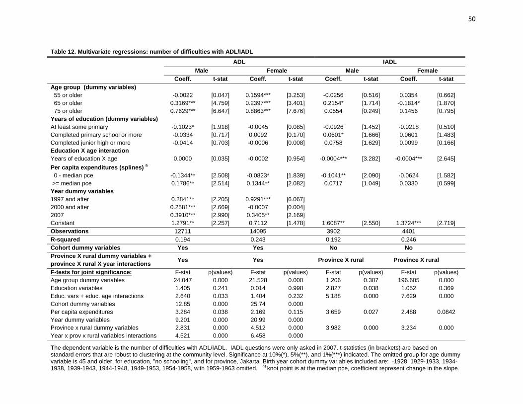
50 

 

Table 12. Multivariate regressions: number of difficulties with ADL/IADL ADL IADL Male Female Male Female Coeff. t-stat Coeff. t-stat Coeff. t-stat Coeff. t-stat Age group (dummy variables) 55 or older -0.0022 [0.047] 0.1594*** [3.253] -0.0256 [0.516] 0.0354 [0.662] 65 or older 0.3169*** [4.759] 0.2397*** [3.401] 0.2154* [1.714] -0.1814* [1.870] 75 or older 0.7629*** [6.647] 0.8863*** [7.676] 0.0554 [0.249] 0.1456 [0.795] Years of education (dummy variables) At least some primary -0.1023* [1.918] -0.0045 [0.085] -0.0926 [1.452] -0.0218 [0.510] Completed primary school or more -0.0334 [0.717] 0.0092 [0.170] 0.0601* [1.666] 0.0601 [1.483] Completed junior high or more -0.0414 [0.703] -0.0006 [0.008] 0.0758 [1.629] 0.0099 [0.166] Education X age interaction Years of education X age 0.0000 [0.035] -0.0002 [0.954] -0.0004*** [3.282] -0.0004*** [2.645] Per capita expenditures (splines) a 0 - median pce -0.1344** [2.508] -0.0823* [1.839] -0.1041** [2.090] -0.0624 [1.582] >= median pce 0.1786** [2.514] 0.1344** [2.082] 0.0717 [1.049] 0.0330 [0.599] Year dummy variables 1997 and after 0.2841** [2.205] 0.9291*** [6.067] 2000 and after 0.2581*** [2.669] -0.0007 [0.004] 2007 0.3910*** [2.990] 0.3405** [2.169] Constant 1.2791** [2.257] 0.7112 [1.478] 1.6087** [2.550] 1.3724*** [2.719] Observations 12711 14095 3902 4401 R-squared 0.194 0.243 0.192 0.246 Cohort dummy variables Yes Yes No No Province X rural dummy variables + province X rural X year interactions Yes

Yes

Province X rural Province X rural

F-tests for joint significance: F-stat p(values) F-stat p(values) F-stat p(values) F-stat p(values) Age group dummy variables 24.047 0.000 21.528 0.000 1.206 0.307 196.605 0.000 Education variables 1.405 0.241 0.014 0.998 2.827 0.038 1.052 0.369 Educ. vars + educ. age interactions 2.640 0.033 1.404 0.232 5.188 0.000 7.629 0.000 Cohort dummy variables 12.85 0.000 25.74 0.000 Per capita expenditures 3.284 0.038 2.169 0.115 3.659 0.027 2.488 0.0842 Year dummy variables 9.201 0.000 20.99 0.000 Province x rural dummy variables 2.831 0.000 4.512 0.000 3.982 0.000 3.234 0.000 Year x prov x rural variables interactions 4.521 0.000 6.458 0.000

The dependent variable is the number of difficulties with ADL/IADL. IADL questions were only asked in 2007. t-statistics (in brackets) are based on standard errors that are robust to clustering at the community level. Significance at 10%(*), 5%(**), and 1%(***) indicated. The omitted group for age dummy variable is 45 and older, for education, "no schooling", and for province, Jakarta. Birth year cohort dummy variables included are: -1928, 1929-1933, 1934-1938, 1939-1943, 1944-1948, 1949-1953, 1954-1958, with 1959-1963 omitted. a) knot point is at the median pce, coefficient represent change in the slope.

51 

 

Figure 12. CES-D 10 Scores by Age and Years of Education, Age 45+, 2007  

33.

54

4.5

CES

-D S

core

40 50 60 70 80Age

MaleFemale

Age 45+, 2007

   

2.5

33.

54

4.5

CES

-D S

core

0 2 4 6 8 10 12Years of Education, 2007

MaleFemale

Age 45+, 2007

52 

 

Table 13. Means and Standard Deviations of CES-D 10 Scores of Adult 25+ Age groups CES-D score Men Women 25-44 years Mean 3.90 3.81 Standard deviation 3.40 3.54 Observations 6,630 6,986 45-54 years Mean 3.52 4.15 Standard deviation 3.10 3.45 Observations 1,882 2,119 55-64 years Mean 3.65 4.29 Standard deviation 3.02 3.28 Observations 1,086 1,191 65-74 years Mean 4.13 4.74 Standard deviation 2.98 3.67 Observations 677 778 75+ years Mean 4.74 5.34 Standard deviation 3.36 3.56 Observations 255 301 45+ years Mean 3.73 4.36 Standard deviation 3.10 3.46 Observations 3,911 4,409 Source IFLS4 Observations are weighted using individual sampling weights.

53 

 

Table 14. Multivariate regressions: CES-D 10 Score

CES-D 10 Score Male Female Coeff. t-stat Coeff. t-stat Age group (dummy variables) 55 or older 0.0079 [0.072] -0.0339 [-0.267] 65 or older 0.3820*** [2.764] 0.2343 [1.466] 75 or older 0.3821* [1.786] 0.4508** [2.106] Education X age interaction At least some primary 0.0168 [0.087] 0.0855 [0.523] Completed primary school or more 0.2515* [1.659] -0.0564 [-0.309] Completed junior high or more 0.0476 [0.228] -0.1116 [-0.463] Education X age interaction Years of education X age -0.0017*** [-3.522] -0.0014** [-2.272] Per capita expenditures (splines) a 0 - median pce -0.2129 [-1.305] -0.0994 [-0.583] >= median pce 0.0791 [0.336] -0.0002 [-0.001] Constant 6.8351*** [3.307] 5.5654** [2.575] Observations 3901 4402 R-squared 0.054 0.055 Cohort dummy variables No No Province X rural dummy variables + province X rural X year interactions

Province X rural Province X rural

F-tests for joint significance: F-stat p(values) F-stat p(values) Age group dummy variables 6.164 0.000 4.205 0.006 Education variables 0.943 0.420 0.361 0.781 Educ. vars + educ. age interactions 10.97 0.000 12.87 0.000 Per capita expenditures 2.147 0.118 0.653 0.521 Province x rural dummy variables 5.337 0.000 9.435 0.000 The dependent variable is the CES-D10 score. The score is computed in the way suggested by the Stanford group that created the CES-D, using numbers from 0 for rarely to 3 for most of the time, for negative questions such as do you feel sad. For positive questions such as do you feel happy, the scoring is reversed from 0 for most of the time to 3 for rarely (see text). CESD-10 module was only asked in 2007. t-statistics (in brackets) are based on standard errors that are robust to clustering at the community level. Significance at 10%(*), 5%(**), and 1%(***) indicated. The omitted group for age dummy variable is 45 and older, for education, "no schooling", and for province, Jakarta. a) knot point is at the median pce, coefficient represent change in the slope.

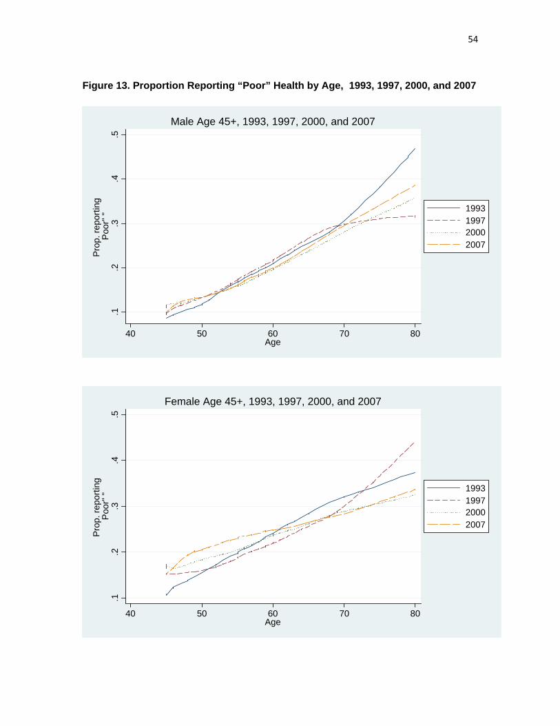
54 

 

Figure 13. Proportion Reporting “Poor” Health by Age, 1993, 1997, 2000, and 2007

.1.2

.3.4

.5

Prop

. rep

ortin

g P

oor"

"

40 50 60 70 80Age

1993199720002007

Male Age 45+, 1993, 1997, 2000, and 2007

.1.2

.3.4

.5

Prop

. rep

ortin

g P

oor"

"

40 50 60 70 80Age

1993199720002007

Female Age 45+, 1993, 1997, 2000, and 2007

55 

 

Table 15. Proportion reporting "somewhat unhealthy" or “unhealthy” to a GHS question, 1993, 1997, 2000, and 2007 Men Women Age groups 1993 1997 2000 2007 1993 1997 2000 2007 25-44 years % reporting "poor" health 6.89 6.65 8.71 10.06 8.62 9.52 11.39 13.17 Observations 2,918 3,667 5,189 6,641 3,679 4,664 5,661 7,000 45-54 years % reporting "poor" health 10.93 12.43 12.98 13.06 14.79 16.32 17.84 20.08 Observations 1,070 1,231 1,487 1,883 1,237 1,342 1,575 2,122 55-64 years % reporting "poor" health 21.26 20.88 18.16 18.20 23.62 21.75 22.33 24.71 Observations 823 953 1,052 1,088 885 1,122 1,272 1,194 65-74 years % reporting "poor" health 27.49 31.50 27.55 28.34 31.19 26.82 29.14 27.64 Observations 451 508 628 681 404 548 731 785 75+ years % reporting "poor" health 38.28 30.77 36.10 35.04 35.64 45.41 31.49 32.24 Observations 128 195 277 254 101 185 289 304 45+ years % reporting "poor" health 18.81 19.81 19.08 18.59 21.09 21.71 22.47 23.52 Observations 2,472 2,887 3,444 3,906 2,627 3,197 3,867 4,405 Source: IFLS1, IFLS2, IFLS3, and IFLS4 Observations are weighted using individual sampling weights.

56 

 

Table 16. General Health Status General Health Status Male Female Coeff. t-stat Coeff. t-stat Age group (dummy variables) 55 or older 0.0310** [2.452] 0.0107 [0.797] 65 or older 0.0660*** [4.206] -0.0193 [1.218] 75 or older 0.0455** [2.141] 0.0065 [0.311] Years of education (dummy variables) At least some primary 0.0115 [0.825] 0.0391*** [2.969] Completed primary school or more 0.0098 [0.774] 0.0139 [0.940] Completed junior high or more 0.0012 [0.078] 0.0115 [0.554] Education X age interaction Years of education X age -0.0001*** [2.683] -0.0002*** [2.979] Per capita expenditures (splines) a -0.0342*** -0.0110 0 - median pce -0.0342*** [2.753] -0.0110 [0.896] >= median pce 0.0259 [1.518] 0.0232 [1.390] Year dummy variables 1997 and after 0.1297*** [4.100] 0.1251*** [3.538] 2000 and after 0.0586** [2.011] 0.0114 [0.291] 2007 0.0387 [1.095] 0.1378*** [3.720] Constant 0.4254*** [3.129] 0.1616 [1.212] Observations 12705 14094 R-squared 0.081 0.064 Cohort dummy variables Yes Yes Province X rural dummy variables + province X rural X year interactions Yes

Yes

F-tests for joint significance: F-stat p(values) F-stat p(values) Age group dummy variables 7.493 0.014 0.989 0.398 Education variables 0.494 0.687 3.360 0.019 Educ. vars + educ. age interactions 6.254 0.014 5.095 0.001 Cohort dummy variables 2.639 0.011 7.259 0.014 Per capita expenditures 5.913 0.003 1.215 0.298 Year dummy variables 10.71 0.014 15.03 0.014 Province x rural dummy variables 4.102 0.014 5.608 0.000 Year x prov x rural variables interactions 3.650 0.000 4.181 0.000 The dependent variable is a binary variable equals to 1 when an individual answers “somewhat unhealthy” and “unhealthy” to the question “In general how is your health” (see text), and 0 otherwise. t-statistics (in brackets) are based on standard errors that are robust to clustering at the community level. Significance at 10%(*), 5%(**), and 1%(***) indicated. The omitted group for age dummy variable is 45 and older, for education, "no schooling", and for province, Jakarta. Birth year cohort dummy variables included are: -1928, 1929-1933, 1934-1938, 1939-1943, 1944-1948, 1949-1953, 1954-1958, with 1959-1963 omitted. a) knot point is at the median pce, coefficient represent change in the slope.

57 

 

Figure 14. Currently Smoking, Male 45+, 1993, 1997, 2000, and 2007  

.5.6

.7.8

Prop

ortio

n

45 50 60 70 80Age

1993199720002007

Currently Smoke: Male Age 45+, 1993, 1997, 2000, and 2007

  

58 

 

  Table 17. Percentage of adults 25+ ever and currently smoke cigarettes or cigars 1993, 1997, 2000, and 2007 Men Women Age groups 1993 1997 2000 2007 1993 1997 2000 2007 25-44 years % ever smoked 75.12 76.78 75.05 73.97 3.15 2.68 2.26 1.75 % currently smoke 70.92 73.34 70.50 70.68 2.63 2.22 2.05 1.42 Observations 3,202 3,288 4,980 6,447 3,749 4,466 5,574 6,904 45-54 years % ever smoked 82.84 79.37 75.65 77.82 7.71 5.70 5.05 3.69 % currently smoke 77.75 72.99 70.10 71.19 7.45 5.33 4.59 3.29 Observations 1,182 1,152 1,460 1,856 1,313 1,283 1,559 2,097 55-64 years % ever smoked 83.45 81.59 81.94 75.21 10.88 7.72 7.96 4.15 % currently smoke 74.40 72.44 70.28 66.43 8.99 6.74 6.90 3.07 Observations 900 889 1,026 1,070 1,017 1,075 1,251 1,181 65-74 years % ever smoked 82.74 85.27 82.95 80.04 8.74 7.63 7.54 8.21 % currently smoke 72.52 68.15 67.43 63.92 6.26 6.97 5.40 6.27 Observations 530 476 615 674 560 511 718 778 75+ years % ever smoked 81.90 81.97 79.31 81.16 6.44 8.34 7.12 5.59 % currently smoke 65.61 69.84 60.90 66.50 4.14 7.76 5.95 4.70 Observations 197 188 273 249 252 175 277 302 45+ years % ever smoked 82.95 81.32 79.19 77.70 8.82 6.89 6.63 4.75 % currently smoke 74.84 71.74 68.92 68.29 7.47 6.24 .60 3.86 Observations 2,809 2,705 3,374 3,849 3,142 3,044 3,805 4,358 Source: IFLS1, IFLS2, IFLS3, and IFLS4 Observations are weighted using individual sampling weights.  

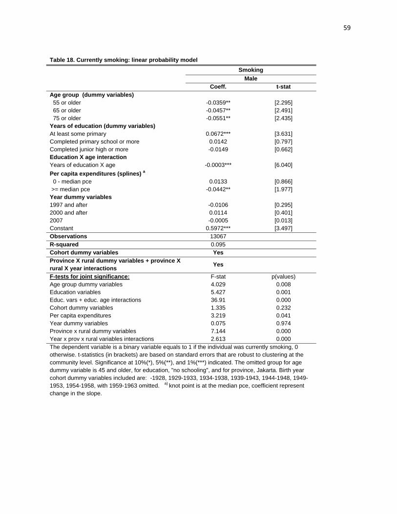
59 

 

Table 18. Currently smoking: linear probability model Smoking Male Coeff. t-stat Age group (dummy variables) 55 or older -0.0359** [2.295] 65 or older -0.0457** [2.491] 75 or older -0.0551** [2.435] Years of education (dummy variables) At least some primary 0.0672*** [3.631] Completed primary school or more 0.0142 [0.797] Completed junior high or more -0.0149 [0.662] Education X age interaction Years of education X age -0.0003*** [6.040] Per capita expenditures (splines) a 0 - median pce 0.0133 [0.866] >= median pce -0.0442** [1.977] Year dummy variables 1997 and after -0.0106 [0.295] 2000 and after 0.0114 [0.401] 2007 -0.0005 [0.013] Constant 0.5972*** [3.497] Observations 13067 R-squared 0.095 Cohort dummy variables Yes Province X rural dummy variables + province X rural X year interactions Yes

F-tests for joint significance: F-stat p(values) Age group dummy variables 4.029 0.008 Education variables 5.427 0.001 Educ. vars + educ. age interactions 36.91 0.000 Cohort dummy variables 1.335 0.232 Per capita expenditures 3.219 0.041 Year dummy variables 0.075 0.974 Province x rural dummy variables 7.144 0.000 Year x prov x rural variables interactions 2.613 0.000 The dependent variable is a binary variable equals to 1 if the individual was currently smoking, 0 otherwise. t-statistics (in brackets) are based on standard errors that are robust to clustering at the community level. Significance at 10%(*), 5%(**), and 1%(***) indicated. The omitted group for age dummy variable is 45 and older, for education, "no schooling", and for province, Jakarta. Birth year cohort dummy variables included are: -1928, 1929-1933, 1934-1938, 1939-1943, 1944-1948, 1949-1953, 1954-1958, with 1959-1963 omitted. a) knot point is at the median pce, coefficient represent change in the slope.

60 

 

 Figure 15. Proportion of Age 45+ Engaging in Continuous Vigorous and Moderate Physical Activity for at Least 10 Minutes in the Last Week, by Education  

.1.2

.3.4

.5Pr

opor

tion

enga

ged

in v

igor

ous

activ

ity

0 1 2 3 4 5 6 7 8 9 10 11 12Years of Education

MaleFemale

Vigorous physical activity, Age 45+, 2007

  

.65

.7.7

5.8

Prop

ortio

n en

gage

d in

mod

erat

e ac

tivity

0 1 2 3 4 5 6 7 8 9 10 11 12Years of Education

MaleFemale

Moderate physical activity, Age 45+, 2007

61 

 

Table 19. Proportion of adult 25+ engaging in vigorous or moderate physical activity continuously for at least 10 minutes in previous week, 2007

Vigorous Moderate Age groups Male Female Male Female 25-44 years % engaged in physical activity 52.58 17.57 83.09 83.31 Observations 6,447 6,904 6,447 6,904 45-54 years % engaged in physical activity 48.21 22.66 80.40 82.49 Observations 1,856 2,097 1,856 2,097 55-64 years % engaged in physical activity 44.68 17.27 78.17 72.29 Observations 1,070 1,181 1,070 1,181 65-74 years % engaged in physical activity 35.15 13.32 69.37 65.68 Observations 674 778 674 778 75+ years % engaged in physical activity 24.19 5.43 53.04 41.33 Observations 249 302 249 302 45+ years % with any difficulty 43.39 18.34 76.08 73.87 Observations 3,849 4,358 3,849 4,358

Source: IFLS4 Observations are weighted using individual sampling weights.

62 

 

Table 20. Physical activities: linear probability models Vigorous Physical Activity Moderate Physical Activity Male Female Male Female Coeff. t-stat Coeff. t-stat Coeff. t-stat Coeff. t-stat Age group (dummy variables) 55 or older -0.0386** [-2.126] -0.0717*** [-5.056] -0.0251 [-1.626] -0.0962*** [-6.369] 65 or older -0.1070*** [-4.928] -0.0646*** [-4.102] -0.1104*** [-5.204] -0.0597*** [-2.744] 75 or older -0.1702*** [-5.157] -0.0811*** [-5.246] -0.2005*** [-5.563] -0.2549*** [-7.919] Years of education (dummy variables) At least some primary 0.0958*** [3.461] -0.0318 [-1.472] 0.0285 [1.096] 0.0484** [2.267] Completed primary school or more -0.0260 [-1.042] -0.0127 [-0.621] 0.0082 [0.364] 0.0487** [2.127] Completed junior high or more -0.0514* [-1.679] -0.0463* [-1.872] -0.0160 [-0.554] 0.0225 [0.743] Education X age interaction Years of education X age -0.0003*** [-4.795] -0.0000 [-0.736] -0.0001 [-0.893] -0.0002* [-1.840] Per capita expenditures (splines) a 0 - median pce -0.0631** [-2.539] -0.0188 [-0.887] -0.0551*** [-2.664] -0.0155 [-0.739] >= median pce 0.0132 [0.378] 0.0153 [0.515] 0.0475 [1.368] 0.0036 [0.116] Constant 1.1808*** [3.745] 0.4743* [1.755] 1.3481*** [4.933] 1.0155*** [3.806] Observations 3902 4403 3902 4403 R-squared 0.153 0.076 0.092 0.127 Cohort dummy variables No No No No Province X rural dummy variables + province X rural X year interactions Province X rural Province X rural Province X rural Province X rural

F-tests for joint significance: F-stat p(values) F-stat p(values) F-stat p(values) F-stat p(values) Age group dummy variables 39.938 0.000 55.739 0.000 37.555 0.000 62.699 0.000 Education variables 6.968 0.000 1.426 0.234 0.873 0.455 3.114 0.0260 Educ. vars + educ. age interactions 36.00 0.000 9.960 0.000 1.243 0.292 2.476 0.0436 Per capita expenditures 10.07 0.000 0.606 0.546 4.732 0.00924 0.794 0.453 Province x rural dummy variables 6.138 0.000 6.276 0.000 7.707 0.000 10.15 0.000 The dependent variable is a binary variable equals to 1 if the individual engaged in vigorous (moderate) physical activities in the past week, and 0 otherwise (see text). Questions about physical activities were only asked in 2007. t-statistics (in brackets) are based on standard errors that are robust to clustering at the community level. Significance at 10%(*), 5%(**), and 1%(***) indicated. The omitted group for age dummy variable is 45 and older, for education, "no schooling", and for province, Jakarta. a) knot point is at the median pce, coefficient represent change in the slope.