Social Status, Land Rights

and Rural-Urban Migration:

The Case of China.

de la Rupelle Maelys ∗

Deng Quheng†

Li Shi‡

Vendryes Thomas §

Preliminary - Please do not quote - Comments welcome

Abstract

Present-day China experiences huge rural-urban migration flows. One strikingcharacteristic of these flows is their high geographical and temporal mobility. Inparticular, rural-urban migrants keep going back and forth between origin and des-tination areas. Usual explanations are the institutional constraints on populationmoves, embedded in the hukou registration system, and agricultural production sea-sonality. However, in China, rural household rights on land are quite insecure, forvillage land property remains collective. In such a context, a household neglectingher land or out migrating faces the risk of being deprived of her rights. However,the intensity of this risk is modulated by her social status, or the influence she candisplay to assert her rights and defend her interests. Social status should thus havea direct impact on migration decision, and especially on the migration duration thehousehold can afford without her land rights being jeopardized.

JEL Classification: J43, L14, Q15, R23.Keywords: social status, rural-urban migration, insecure land rights.

∗PSE (Paris-Jourdan Sciences Economiques/Paris School of Economics), 48 boulevard Jourdan, 75014Paris, France. Email: rupelle@pse.ens.fr, phone: (+33)143136314.

†CASS (Chinese Academy of Social Sciences), Yuetan Beixiaojie, Beijing 100732, China. Email:qhdeng@vip.sina.com

‡Beijing Normal University, 19 Xinjiekouwai Street, 100875 Beijing, China. Email : lishi@bnu.edu.cn§PSE (Paris-Jourdan Sciences Economiques/Paris School of Economics), 48 boulevard Jourdan, 75014

Paris, France. Email: vendryes@pse.ens.fr, phone: (+33)143136393.

1

1 Introduction

Rural-Urban Migrations in China

From 1978 on, the reform and opening policies first promoted by Deng Xiaoping have led

the People’s Republic of China into a path of rapid economic growth and sharp social

changes. These policies progressively allowed some spreading of market processes, espe-

cially regarding the allocation of production factors (labor, land and capital). Even if

markets still remain far from complete and quite highly constrained, this partial liberal-

ization has given rise to a high pace of capital accumulation, and to a geographical and

sectoral redistribution of Chinese workforce. In particular, China has been experienc-

ing increasing migration flows of laborers from rural agricultural areas to industrialized

cities. Though it is hard to exactly count the number of these migrant rural workers, for

they are usually highly mobile and often live on the fringes of legality, existing studies

converge to a commonly accepted estimate of the growth in size of this population from

around 2 millions in the mid-1980s to about 94 millions in 2002. It would mean that,

at the beginning of the xxist century, rural-urban migration affected as much as 12 % of

total Chinese workforce, and almost a fifth of the rural active population.1

Who are the Migrants?

All empirical studies point to the particular features of this migrant population2, that one

will find in most internal migrant population elsewhere in the world: Chinese rural-urban

migrants are mostly young, in their 20s, predominantly male, and they tend to be more

educated than their fellow countrymen who do not migrate. Moreover, they are poor

people from poor regions, but not the poorest of the poorest. Migration induces a cost

that the poorest cannot afford; on the other hand, migrants job are not lucrative enough

for the richest rural inhabitants.

The very rich dataset we are using confirms this rural-urban migrant population struc-

ture. We use a survey conducted by CASS in 2003. It has been conducted during 2003

Spring Festival, and inquired the situation of rural households the preceding year. This

survey has three main advantages. First, the set of questions was quite comprehensive,

and deals with a large number of aspects of rural household life. Second, the survey

relies on a very wide sample: 37 969 people distributed across 22 provinces3 have been

interviewed. Third, and last but not least, it was conducted during the Spring Festival, a

time of traditional familial gathering, and therefore a lot of migrants had returned their

hometown for the occasion and were present. These three reasons give this survey much

interest for the study of Chinese internal migration.

A core element is the definition of migration. Migration is usually defined in relation

1See for example Huang and Pieke (2003)2See, for instance, Zhao (1999)3The provinces sampled are the following: (listed from East to West, and from North to South)

Jilin, Liaoning, Beijing, Hebei, Shandong, Jiangsu, Zhejiang, Guangdong, Shanxi, Henan, Anhui, Hubei,Jiangxi, Hunan, Shaanxi, Chongqing, Guizhou, Guangxi, Xinjiang, Gansu, Sichuan, Yunnan.

2

with two criteria: place of work, and length of work. The National Bureau of Statistics

defines a migrant as an active individual who has left his place of registration to work, at

least for 6 months. For the purpose of this study, we define as a migrant any individual

who says that he worked out of his usual place of residence during the past year. The only

restriction we put on this definition is that the place of work must be not only out the

individual’s home village, but out of the individual’s home county. Indeed, township can

be quite small, and there could be a lot of commuters among people working outside the

township but living within the village. In 2002, there were 44 850 township-level divisions,

and 2 860 county level divisions. China as a whole is 9,33 million square kilometers. So

townships are in average a little bit more than 200 square kilometers while counties are

in average more than 3 260 square kilometers. In rural area the average area is slightly

bigger, but the difference between those two hierarchical levels remains huge. It follows

from these geographical data that workers who stay inside a county can quite easily be

commuters, and as such are not included in our definition of migrant people.

So finally, how many migrants can we identify in the data? According to the survey

(see table 1), 15,4 % of active people have worked outside their county in 2002. That

is, 9 % of the rural population are migrant workers. If we assume that the people are

well sampled, then that means that 9% of the 853,24 millions of rural people living

in the sampled provinces are migrants,and then 82,6 millions of people have left their

rural household to work outside their county in 2002. If we further suppose that the 22

provinces of our sample are representative of China general situation, then it would mean

that 93 millions of rural people have migrated in 20024. That fits with previous estimates

of the size of the floating population.

Place of work Percent of active people

Within village 16,55

Outside village, within township 10,31

Outside township, within county 5,59

Outside county, within province 6,78

Outside province 8,10

Agricultural work - Place of work missing 52,68

Total 100%

Table 1: Place of work of active people

67 % of migrants are men, whereas men account for 52% of the population of “stayers”;

results regarding years of education and age are reported in the following table.

The scope of this migration phenomenon in China has naturally aroused much interest

and debates in academic as well as political circles, about its causes, its evolution and

its consequences on economic development and social order. So far, on the micro side,

4On a rural population of 935 025 000 people. All the figures are from Statistical Yearbook (2003),Chapter 12-3, Basic conditions of grass roots units.

3

Table 2: Descriptive statistics on active people

Migrants Non migrants

Variable Mean (Std. Err.) Mean (Std. Err.)

age 28,7 (9,9) 40,2 (12,9)

years of edu. 8,7 (2,5) 7,4 (3,4)

Number of obs. 3404 20425

the related economic literature has been focusing mainly on the specific characteristics of

migrant people, holding the classical Todarian5 point of view that differentials in labor

revenues were the main motive for migrations. Moreover, on the macro side, much of

the political and social debates about Chinese internal migrations seem to rely on the

implicit assumption that this phenomenon is comparable to the “exode rural” that took

place in xixth century industrializing Europe, and in most developing countries during the

xxth century. Rural-urban migrations are thus seen, in a Lewisian way,6 as the necessary

corollary of capital accumulation, industrialization and urbanization.

Temporality of Migrations

However, with such an economic theoretical framework and historical baseline example, it

does not seem possible to account for one of the most striking feature of Chinese migrant

population -namely that it is a “floating population” (liudong renkou). A lot of rural

migrants return home after three, four years of migration. But that alone doesn’t explain

why they are said to be “floaters”. The point is that, during a single year, migrants

are likely to change occupation, to move from one place to another, and to come back

farming during the peak season. This is this second aspect we would like to consider.

It is very clear, in our data, that quite often, out-migration lasts for less than one year.

Among the migrant population, half of the people came back to participate in farming

activities in 2002, and almost 60% of them, as table 3 shows, came back for at least three

months in their home village.

Length of migration during 2002 %

Less than 3 months 12,5

Between 3 and 6 months 20,3

Between 6 and 9 months 25,5

More than 9 months 41,6

Total 100

Table 3: Length of migration

Migrant people in China well deserve their ”floating population” label.

5See Todaro (1969) and Harris and Todaro (1970).6See Lewis (1954).

4

The theoretical literature on temporary migration is quite scarce. By focusing on

Chinese case, we hope to bring new elements to the literature on migration duration as

well. In such a literature, return within a year or after many years usually responds

to four main reasons. The first one may be a change in revenue differential between

origin and destination area. A peculiar reason for temporary migration within a year

is agricultural seasonality, which is quite momentous in Chinese agriculture.7 Secondly,

return can be the consequence of an exogenous shock, as in Galor and Stark (1990): the

instability of informal labor markets and the frailty of administrative situation of many

undocumented migrants can force some of them to return home. Thirdly, return can

be motivated by psychological and family ties. As time goes by, the cost for being far

way from home and family increases. Technically, in this case, it is usual to assume

that consumption at home brings a higher utility than consumption at the migrant’s

destination. In most works on migration duration8, that’s why migrant has an incentive

to return home. But this back-pulling force is assumed rather than explained. The fourth

and last reason behind temporary migration is the necessity for a household to diversify

risk among sectors and localities9. In that framework, people leave for cities in order to

cope with a volatile agricultural income. Migration, here, is an insurance device.

Those explanations might all play a role in Chinese internal migration. But they

are imperfect. The seasonality in agriculture is high in China. However, farming work,

even during peak season, might be less profitable than migration. In that case, return

migration probably yields other outcomes. Those outcomes may be linked with the

diversification of risks issue. In that framework, household chooses to allocate her labour

force as one decides to allocate a portfolio of options. In most literature on migration

and risk, it is usually assessed that the migrant will provide to her household liquidities

to cope with climatic hazard on agricultural production. Similar mechanism operates at

the individual level, but in the opposite direction: the individual regularly returns to the

home rural area, for it ensures her a future flow of income. Indeed, migrants jobs are

very instable, and rural migrants, because of their peculiar status, are deprived of social

security and, very often, of formal job contracts. Their land may be the only insurance

asset they have.

However, even if rural households have been granted use rights on land, officially in a

contractual framework, real property rights have remained in the hands of the collective.

That means that household’s land can be administratively redistributed. Actually, village

authorities, in most localities, have taken the habit of periodically reallocating land among

fellow villagers.10 If a reallocation occurs, migrants’ land can be taken away to the benefit

of those living in the village. This leads to our first hypothesis: land evolution influences

the migration decision. (H1). Before going further, we need to understand the way land

evolves, and to empirically check whether it impacts migration decision.

7See Knight and Song (1997) and Aubert and Li (1998).8See for instance Djajic and Milbourne (1988), Dustmann (2003) and Mesnard (2004).9See Stark and Levhari (1982) and Stark and Bloom (1985).

10See for example Kung and Liu (1997).

5

The Land Rights Issue

In the late seventies, when the Household Responsibility System has been implemented,

land has been allocated on a individual basis. Three main rules of reallocation have been

followed. The first one was according to household size. The second one was according to

household number of laborers. The third one was a combination of the two others. The

first rule was broadly used, and preferred by poor villages, whereas richer area tended to

follow the other ones. 11

Then, demographic change and economic pressure led to many land reallocations. A

survey conducted in 2005 among 3000 households12 indicates that more than 74% villages

have reallocated their land since the introduction of the Household Responsibility System.

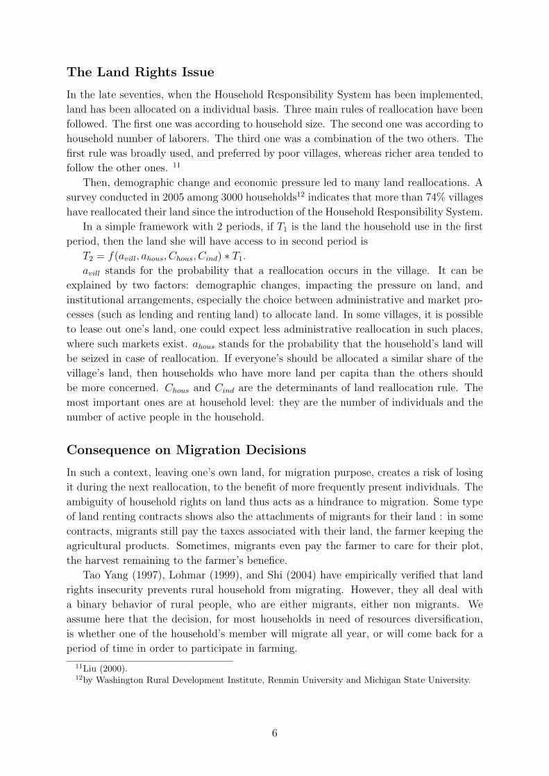
In a simple framework with 2 periods, if T1 is the land the household use in the first

period, then the land she will have access to in second period is

T2 = f(avill, ahous, Chous, Cind) ∗ T1.

avill stands for the probability that a reallocation occurs in the village. It can be

explained by two factors: demographic changes, impacting the pressure on land, and

institutional arrangements, especially the choice between administrative and market pro-

cesses (such as lending and renting land) to allocate land. In some villages, it is possible

to lease out one’s land, one could expect less administrative reallocation in such places,

where such markets exist. ahous stands for the probability that the household’s land will

be seized in case of reallocation. If everyone’s should be allocated a similar share of the

village’s land, then households who have more land per capita than the others should

be more concerned. Chous and Cind are the determinants of land reallocation rule. The

most important ones are at household level: they are the number of individuals and the

number of active people in the household.

Consequence on Migration Decisions

In such a context, leaving one’s own land, for migration purpose, creates a risk of losing

it during the next reallocation, to the benefit of more frequently present individuals. The

ambiguity of household rights on land thus acts as a hindrance to migration. Some type

of land renting contracts shows also the attachments of migrants for their land : in some

contracts, migrants still pay the taxes associated with their land, the farmer keeping the

agricultural products. Sometimes, migrants even pay the farmer to care for their plot,

the harvest remaining to the farmer’s benefice.

Tao Yang (1997), Lohmar (1999), and Shi (2004) have empirically verified that land

rights insecurity prevents rural household from migrating. However, they all deal with

a binary behavior of rural people, who are either migrants, either non migrants. We

assume here that the decision, for most households in need of resources diversification,

is whether one of the household’s member will migrate all year, or will come back for a

period of time in order to participate in farming.

11Liu (2000).12by Washington Rural Development Institute, Renmin University and Michigan State University.

6

Indeed, if mobility becomes an important characteristic of rural population, the notion

of “rural active individual” itself may be hard to define.

Do migrants come back home to participate in planting because they fear a

reallocation?

Among migrants, what characteristics distinguish those who come back from the others?

Half of the migrants come back to participate in agricultural work. To better picture

out their characteristics, the probability of coming back for a migrant whose household

cultivates land is regressed on a set of:

• individual controls (age squared, marital status, sex, years of education);

• household level variables: access to water, as a measure of poverty; (three possibil-

ities : private tap, motor-pumped well, or natural well); age mean, as an indicator

of life-cycle position; land per capita ;

• variables linked with the possible evolution of land.

We introduce variables likely to impact land evolution through reallocation. They are

the different arguments of the function f(.) described above.

The variables avill, the village level variables, consist here of two dummies, which are

inversely correlated with the probability of reallocation. The first one is demographic, and

indicates whether the village population has decreased during the past year (which means

more deaths than births, or departure of rural people who obtained an urban hukou).

The other one indicates that an informal land market exists in village; it equals one when

some households are lending out their land or leasing in it from others households.

For the remaining arguments, ahous and C(.) variables, we do not know how they

interact with each others. We therefore construct a measure of the threat the household

faces in case of land reallocation. The allocation might be made on a land per capita

basis. If land per capita is high in one household, this household might be more subject

to reallocation. Much more than this, if the marginal changes is high when one leaves,

then one departure will more expose the household to reallocation.

We first compute the difference in land per active members if one active left. If this

difference is big, it means two things : the household has a lot of land or the household

has few members. We then look at the distribution of this variable in each county, and

using quintile, we construct five dummies that indicates the place of each household in

terms of marginal land endowment per member. The first level of threat is associated

with the first 25% in the county : people with the smallest changes in term of land per

capita if they leave.

First, we build

Threati =Ti

n∗i − 1

− Ti

n∗i

where n∗i is the number of laborers in my household, except me; ni the household number

of laborers, Ti the land used by household i. We thus have:

7

Threati =Ti

n∗i (n

∗i − 1)

If it had been possible, we would have chosen the village as reference for quintile

definition, and not the county, since the land is owned and managed at the village level.

Unfortunately, data give us only a small sample in each village : 10 households. Measure-

ment error and selection bias may be important within such a small sample. Therefore,

we assume that county level variable could give us sufficient information about pressure

on someone’s land. Another argument makes the county an interesting level of analysis.

Indeed, our migration variable is defined on a county basis. We could expect that ap-

preciable differences in land availability within county could lead to internal movements

of people, which we do not need to account for here. This variable Threati was then

used to indicate the relative position of one household in the county. The corresponding

regressors are five dummies, reflecting the quintile distribution of the variable of poten-

tial threat on household’s responsibility land. Those five level increase with the level of

threat. In the regression, the reference is individuals around the median, between the

second and the third quintile.

In the regression, the variable Threat appears conditional on the fact that there is no

land market in the village. It impacts the migration decisions only when administrative

reallocation is the most likely to occur.

We thus can get a better picture of who temporary migrants are.We run a first probit

regression of the probability of migration on the set of independant variables. We then

run a probit regression of the probability for migrants to participate in farming on the

same set of variables. We obtain the following results:

First of all, the land per capita is of crucial importance. The higher the land per

capita in a household, the less likely she will be to migrate, but the more likely she will

be to come back and work on the farm if she has migrated. There is no surprising effect

here.

Most dependant variables have their sign changed with the change of the independent

variable. For instance, married people migrate less, and are more likely to work at home

within a year when they migrate. It means that these variables have a similar impact on

the probability for an active to migrate, and on the probability for a migrant to migrate

a long time. Their effect are the same on transitions from non migration to migration,

and from short term migration to one year migration.

Migrants who return home are more likely to be older and married than those who do

not; they also are a little bit less educated. Poverty, measured by access to water, seems

to indicate that people coming back have some basic facilities at home.

As expected, the variable indicating the existence of “land market”, that is of inter

households exchanges and contracts for renting in or out land plots, is found significant. In

those places, administrative reallocation might be less feared, since market arrangements

already take place.

The variables which have not a monotonous impact on the duration of migration are

more questioning. They play a different role once one individual has decided to migrate.

8

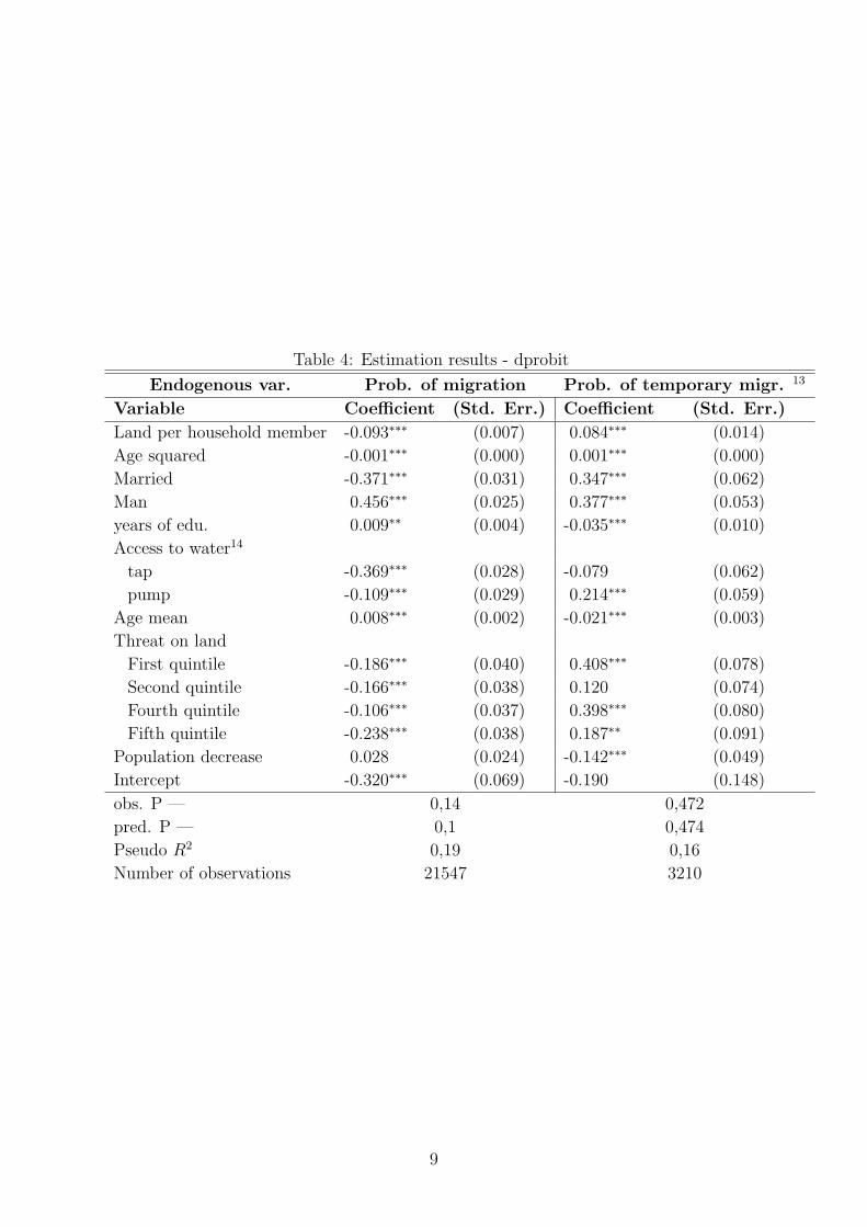
Table 4: Estimation results - dprobit

Endogenous var. Prob. of migration Prob. of temporary migr. 13

Variable Coefficient (Std. Err.) Coefficient (Std. Err.)

Land per household member -0.093∗∗∗ (0.007) 0.084∗∗∗ (0.014)

Age squared -0.001∗∗∗ (0.000) 0.001∗∗∗ (0.000)

Married -0.371∗∗∗ (0.031) 0.347∗∗∗ (0.062)

Man 0.456∗∗∗ (0.025) 0.377∗∗∗ (0.053)

years of edu. 0.009∗∗ (0.004) -0.035∗∗∗ (0.010)

Access to water14

tap -0.369∗∗∗ (0.028) -0.079 (0.062)

pump -0.109∗∗∗ (0.029) 0.214∗∗∗ (0.059)

Age mean 0.008∗∗∗ (0.002) -0.021∗∗∗ (0.003)

Threat on land

First quintile -0.186∗∗∗ (0.040) 0.408∗∗∗ (0.078)

Second quintile -0.166∗∗∗ (0.038) 0.120 (0.074)

Fourth quintile -0.106∗∗∗ (0.037) 0.398∗∗∗ (0.080)

Fifth quintile -0.238∗∗∗ (0.038) 0.187∗∗ (0.091)

Population decrease 0.028 (0.024) -0.142∗∗∗ (0.049)

Intercept -0.320∗∗∗ (0.069) -0.190 (0.148)

obs. P — 0,14 0,472

pred. P — 0,1 0,474

Pseudo R2 0,19 0,16

Number of observations 21547 3210

9

For instance, men are more likely to migrate. But it doesn’t mean they are more likely to

be long term migrant : indeed, they are more often temporary migrants than women. One

reason may be the social pattern behind ( one may think of a family at home with a man

temporarily leaving to bring money back as a paradigmatic pattern of temporary rural

migrant). It could be also that men receive more land in case of reallocation. However,

the first effect is likely to be dominant here. That’s why it is important to control for the

sex of the individual.

More interestingly, found that places were population decreased during the previous

year have no specificities in terms of out migration (variable is not significant in first

regression), but they see less of their migrants coming back. It could indicate that

population decline loosens demographic pressure on land, and that people need less to

come back, for a redistribution, in case it happens, would be less harmful.

But the most interesting variable is the variable of threat on land, that is, the quintile

a household belongs to in term of land per active member, conditional on the absence of

land market in the village. Since the reference is the middle quintile, people close to the

median of the distribution, we see that, if there is no land market, people will migrate

less if they are far from the median.

Then, this effect increases toward both extremes. The direction of the variation

reflects different attitudes according to initial dotations. People with very poor dotation

in term of land per capita will not migrate: they have no land, either because they do

not need to use it (they already have a lucrative option beside farming, and do not need

to migrate), or, more likely, they are the poorest, and they do not have enough money to

migrate. People with very high amount of land are, undoubtedly, the richest among the

farming household. They migrate less, for the richest villagers are well off enough in rural

area, and do not need to migrate. Those elements are quite consistent with all empirical

literature on internal migrants in China. If we now look at the same variable in the other

regression, we find an interesting inter quintile variation. For the individual under the

second quintile, the effect is monotonous. We have a strong disincentive to migrate for

the poorest: we do find the strongest propensity to come back and participate in farming

for them.

The two upper level of potential threat are much more stimulating. First, let us

compare the second and the fourth quintile. They have almost a similar propensity to

migrate in the first regression. But then, although they are both in the middle part of

the distribution regarding land endowments, the absence of land market affects them in

a rather different way. Only the one above the median, much more threatened in case of

reallocation, will have a strong and significant propensity to come back to participate in

farming. And if we look at the last quintile, we find that those people are still more likely

to come back and farm, but twice less than the previous one. It seems here that some

mechanism may temper the need to come back. It could be that land, being abundant in

that household, and land returns thus being small, losing some of it is not really feared.

But it could be, also, that this high dotation in land is associated with some ways of

escaping reallocation. Those household could have enough social status to keep their

land in case of redistribution.

10

All those descriptive characteristics of migrants coming back to farm are fully consis-

tent with our hypothesis. People might come back in order to maintain the size of their

land in case of redistribution. The migrants return might be strongly linked with land

scarcity.

Still, people with much more land than the others are less likely to be migrant than

those who are just above the median. This leads to our second hypothesis: some omitted

variables can protect some people from land seizing. We would like to show that, among

them, social status plays a key role. It’s our second hypothesis : Social status influences

land evolution. (H2)

Social Status

How does social status influence land evolution? Land tenure types are many (five types

can be distinguished), but they do not have the same importance. We will focus here

on the two main ones: the grain ration land, kouliang tian, and the responsibility land,

zeren tian.

When land was first reallocated, the land assigned to meet household basic needs, or

kouliang tian, depended on the household size, and the responsibility land, or zeren tian,

depended on household number of workers. Afterwards, it appeared that the household’s

use rights on her kouliang tian are much more secure than the ones she has on her zeren

tian. Because of its peculiar status, we assume that the kouliang tian is less subject

to reallocations. Household often look at their kouliang tian as their own plot. If it is

the case, these two kinds of land should have different impacts on a rural household’s

decisions.

According to this framework, we should find that the quantity of responsibility land

is correlated with social status, whereas the area of grain ration land is not. Indeed, the

kouliang tian is less likely to have been redistributed. So the area farmed by a household

as ration land is less likely to be the results of negotiations and social bargains. Therefore,

it should reflect the land allocation rule applied when the responsibility system has been

introduced.

One should pay attention to the following point: we are not considering the function

f(.) described above. This function represents the future evolution of land from one

period to an other. Here, we deal with a history of past reallocations, where social

capital is likely to have played a role.

It can be useful to describe the process of land allocation at the very first place, that

is, at the time household responsibility system was implemented. First, the land owned

by a village, T , was divided into small plots, which were then attributed to the P rural

households of the community. Two criteria could have been taken into account for this

allocation: household size mi, household number of workers ni. Allocation could have

been according to one criteria alone or to both of them. So at the time of the introduction

of household responsibility system, the land of household was probably:

Ti = Amγi n

ηi

T

P

11

Since then, reallocations may have occurred. If our hypothesis is valid, then the

current land used by a household should be a function of the size and the number of

laborers she had at the time the reallocation occurs, but also of her social status, because

her social status is likely to have played a role each time a reallocation occurred. The

land the household i owns now can be written as:

Ti = Amγi n

ηi z

1−γ−ηi

T

P

where Z indicates the household social status. It’s quite consistent with the way land

was attributed when the Responsibility System has been introduced. To check whether

our first intuitions are right, we see if the following equation fits our data.

ln(Ti) = ln(Amγi n

ηi z

ζi ) + ln(

T

P)

ln(Ti) = ln(A) + γ ln(mi) + η ln(ni) + ζ ln(zi) + ln(T

P)

Interestingly enough, we know the household size in 1998, and use it as mi. it may

be more accurate, since reallocation might have happen quite a long time ago.

We then observe that household dotation in responsibility land has been influenced

by previous social status indicators.

We use two ways to approximate one household’s social status, both of them displaying

similar effects. The first one indicates that the household had an important status before

the introduction of the household responsibility system, and so, probably, at the time the

land was reallocated. It uses information on household head’s parents. We know what

was the social status of the parents in the time of the land reform. It was called the

chengfen and classified peasants onto 5 categories, namely poor peasant (or landless),

lower middle-peasant, rich-middle peasant, rich peasant, and landlord. We do find that

the households having one rich peasant among the household’s head parents are likely

to use a little bit more land than the others. We assume that the status of rich peasant

might be an indicator of some inherited social status. Since this information is quite old,

we are likely to capture an indicator of social status when reallocation occurred. 8,1% of

the households of our sample belong to such a category.

The second variable standing for social status is a little bit more elaborate. We first

build a social capital measure, by summing up the number of parents of the household

head and head spouse who were labeled as rich peasant in the time of land reform, the

number of parents who were communist, the number of people in one household who

are cadre or work for a governmental administration, and the number of people who got

their job through cadre introduction. We then divide this sum by the corresponding

number at the county level, to get a relative measure of social status (and to correct

for intercounty differences). The dummy we then use equal one when the household

belongs to the highest quartile in term of social status. It has a significant effect. It is

quite surprising, because by construction, this variable uses information on people who

have an off-farm employment, local as well as outside county. Those people not having

agriculture as primary activity, their household should have less land than others. And

the significant effect of this dummy deserves to be stressed.

12

We run the same regression on the quantity of kouliangtian and on the total amount

of land.

Dependant vari-

able : ln(T )

ln(zeren tian) ln(kouliang tian) ln(total land)

Coef. Coef. Coef.

(Std. err.) (Std. err.) (Std. err.)

independant vari-

ables

ln(A) 0,3 — 0,52 — 0,3 —

(0,03) — (0,04) — (0,03) —

ln(mi[1998]) 0,58 — 0,57 — 0,6 —

(0,02) — (0,03) — (0,02) —

ln(ni) 0,12 0,13 0,12 — 0,14 —

(0,02) — (0,02) — (0,02) —

Past social status 0,05 0,006 0,04

(0,02) (0,03) (0,02)

Present social status 0,04 0,02 0,03

(0,016) (0,03) (0,02)

ln(TP) 0,96 — 0,7 — 0,99 —

(0,01 ) — (0,01) — (0,01) —

R2 = R̄2 = 0,46 0,47 0,41 0,41 0,45 0,45

Number of observa-

tions

8204 5268 5268 8224 8224

Table 5: Land repartition

P varies with T , since TP

is the area of each type of land at the county level divided

by the number of people whose household use such type of land. The coefficient of ln(TP)

is not 1, as set in our equation. Indeed, we replaced ln(TP) by its value at the county

level. Error measurement downward biases the coefficient. To find a value of 0.95 is quite

satisfying. It’s even 0,98 when we consider all land. We have check then for model’s

specification by summing the household shares of land in all county. If the specification

of the allocation rule is correct, then the sum should be near to one. It cannot be equal

to one, since we have taken the county level, whereas this rule applies at village level.

Still, we find a mean of 1,7, with values ranging from 0,5 to 4, and with a standard

deviation of 1. For 75 % of the counties, we do find a sum between 0,5 and 2. We could

have constrained the regression, but it had not much sense : anyway, 1998 household size

and actual number of active people differ probably of what they were when the previous

reallocation happened.

Since land allocation obeys to rather egalitarian rule in China, to find an effect of

social status had nothing obvious. So, we have strong reason to believe in our model: the

13

significance of social capital level is quite striking.

So far, we have empirical elements to think that land evolution influences migration

decision, and that social status influences land evolution. The question we would like

to examine in this paper is the following : does the social status influence my migration

decision? We have only fragmented evidence about the link between land evolution and

migration, and between land and social status. Moreover, recall that the two probit on

migrants decisions were made on specific samples, and suffer from selection bias : one

cannot infer, from then, any conclusions for the all population in term of social capital.

For that, we need a unified framework, that could allow us to better understand the

impact of social status on migration decision. That’s the purpose of the following model.

2 The Model

2.1 Setup

General Idea

The main underlying idea of the model we want to design here is that rural households

rights on land are quite insecure, consecutively, when rural households take decisions,

they have to take into account the possible impact of their actions on the evolution of

quantity of land that is granted to them. Here, we design a very simple framework, at

a single village level, to account for the household decision about her optimal migration

duration, under the specific constraint that the time spent out of the village can lead to

a loss of land, but can be compensated by influence on village leaders or fellow villagers.

Grain Ration Land vs Responsibility Land

Actually, Chinese rural households use agricultural land under various land tenure types

and rights. Five major tenure types are officially sanctioned by the national government:15

responsibility land (zeren tian), grain ration land (kouliang tian), contract land (chengbao

tian), private plot (ziliu di) and reclaimed land (kaihuang di).16. Generally speaking, the

property rights on all agricultural land remains in the hands of the village, and there is

thus no form, properly speaking, of private ownership of land. However, each tenure type

encompasses a different set of rights and obligations for rural households, and guarantees

a different level of security. In particular, rural households have almost complete control,

except the right of title transfer, on private plots and grain ration lands, generally without

obligations, whereas responsibility land, contract land and reclaimed land imply various

obligations, such as the delivery of a mandatory quota of grains to the state at below-

market prices, and can be quite easily taken away by collective authorities to be allocated

to other households. To simplify the analysis, we can consider that the last three types of

land can be quite easily transferred and reallocated among households by the collective,

while the first two cannot. Moreover, as in rural areas, private plots are qualitatively

15See Brandt, Huang, Li and Rozelle (2002)16See the aforementioned article for an exact description of these tenure types

14

comparable and quantitatively marginal compared to grain ration land, we will generally

include both types under the label “grain ration land”. For the same reasons, we will

collectively deal with responsibility land, contract land and reclaimed land under the

label “responsibility land”. In our model, we distinguish these two kinds of land tenures,

and deal with “responsibility land” as subject to a threat of reallocation, whereas the

household’s use rights on “grain ration land” can be taken as secure and stable.

The household endowments and life cycle

The village has a limited quantity of land, T , which is seen as exogenously given. It is

populated by N households, indexed by i.

At the beginning, the household i is endowed with a quantity of labor Li1, which

depends on her number of active people. She is also endowed with an overall quantity

of land Ti1, which includes both her “grain ration land”, TGi1, and her “responsibility

land”, TRi1. The first kind of land cannot be lost, reallocated or transferred by the

collective, while the second kind of land is subject to a “threat” of being reallocated. The

household is also endowed with a social status, or social influence zi1, which represents her

social power, the network -the Chinese guanxi - that she can mobilize to assert her rights

and defend her interests. All in all, zi1 embodies the social aura, the social influence

of household i. To simplify the analysis without altering the general intuitions of the

model, Li1 and zi1 remain constant over time. To sum up, the initial endowment of a

rural household is given by the set (Li, zi, TGi1, TRi1).

A household i lives two periods. During the first one, she can decide to migrate, while

in the second one she definitively comes back and settles down in the rural area. That

constraint makes the model much simpler to deal with, and seems to be realistic. Indeed,

for much of Chinese rural individuals and households, migration appears to be a first

step, a first period of their life-cycle, before a definitive return and settling in rural areas.

Moreover, if an individual or a household decides to migrate without keeping the long

term goal of coming back to her origin locality, she will have no reasons, apart from purely

personal and familial ones, to come back regularly to her home town. She will not fit into

the model, but she will also be missing from our rural data. So, for theoretical as well

as empirical reasons, it seems legitimate to constrain the household to be fully involved

in rural activities during the second period. To keep our model simple and tractable, we

thus set this definitive return decision and its timing as exogenous.

First Period

During the first period, the household can choose to allocate the labor of her workers to

the rural activity and to migration. We assume that the rural activity involves the use of

land and labor, and that the household acts as a private entrepreneur. So the household

gets the following revenues:17

• The rural activity yields a revenue F (TG1 + TR1, LT1)

17We get rid of the i as we study only one household.

15

• Migration provides with a total income LM1wM(X)

Where:

• LT1 and LM1 respectively denote the time spent on working in the rural area, and

migrating. We have of course: LT1 + LM1 = L, and in particular, LM1 = L− LT1,

• X denotes the individual characteristics that are valued in the urban labor market,

• Incomes are evaluated at their monetary value.

All in all, the household first period income can be expressed as a function of LM1, and

is given by:

W1(LM1) = F (TG1 + TR1, L− LM1) + LM1wM(X) (1)

There is no saving, and so her first period consumption is given by:18

C1(LM1) = W1(LM1) = F (TG1 + TR1, L− LM1) + LM1wM(X) (2)

Second Period

During the second period, the household cannot migrate, her income is thus generated

through the rural activity, which yields a revenue F (T2, LT2), with:

• LT2 = L,

• T2 = TG2 + TR2 = TG1 + f(z, L− LM1)TR1,

The main idea here is that responsibility land is subject to reallocation, while grain

ration land is not. For a given household, the quantity of responsibility land that has

been granted to her can evolve from a period to another. Social status or influence z is

a way of defending her rights and influencing the evolution of her quantity of land, as

is the time spent in the rural area L − LM1. The function f(.) reflects this evolution

of the quantity of land granted to the household, and how she can deal with it through

her local influence, which depends on the social status and the time spent in the rural

area.19 This function f(.) is assumed to be increasing in her arguments, and to display

decreasing returns.

Second period income and consumption thus are:

C2 = W2 =F (T2, LT2)

=F (TG1 + f(z, L− LM1)TR1, L) (3)

18Utility is seen as linear in the consumption.19We will discuss later more accurate specifications for f(.), taking into account other characteristics

of the households.

16

2.2 The Household Migration Decision

Finally, the objective of the rural household is to maximize her intertemporal consump-

tion, which equals her intertemporal utility, with a discount rate taken as equal to one.

Using (2), (3) and the expression of T2, this consumption is:

C =W1 + W2

=F (T1, L− LM1) + LM1wM (4)

+ F (TG1 + f(z, L− LM1)TR1, L)

The household will maximize this intertemporal objective function in LM1, that is she

will decide the optimal allocation of the labor of her members.

So, all in all, the maximization program of the household is:

maxLM1

C =F (TG1 + TR1, L− LM1) + LM1wM (5)

+ F (TG1 + f(z, L− LM1)TR1, L)

s.t. LM1 ≥ 0

Optimal Allocation of Labor and Optimal Migration Duration

The Lagrangian related to the above mentioned maximization program is:

Λ(LM1, λ) = F (TG1+TR1, L−LM1)+LM1wM +F (TG1+f(z, L−LM1)TR1, L)+λLM1 (6)

The first order condition is:

∂Λ(LM1, λ)

∂LM1

= 0

− ∂F

∂LT

(T1, L− LM1) + wM − ∂f

∂LT

(z, L− LM1)TR1∂F

∂T(TG1 + f(z, L− LM1)TR1, L) + λ = 0

(7)

If λ 6= 0, then LM1 = 0 and ∂F∂LT1

(T1, L) + ∂f∂LT1

(z, L)TR1∂F∂T

(TG1 + f(z, L)TR1, L) ≥wM . It is more profitable for the household to spend all her working time to the rural

area, because the marginal productivity of her rural labor, concerning both first period

production production and the evolution in her quantity of land, stays always higher than

migration marginal income, that is the urban informal sector wage.

If λ = 0, then LM1 ≥ 0, and the optimal migration duration L∗M1 is such that:

− ∂F

∂LT1

(T1, L− L∗M1) + wM − ∂f

∂LT1

(z, L− L∗M1)TR1

∂F

∂T(TG1 + f(z, L− L∗

M1)TR1, L) = 0

In this case, the marginal income of migration, ie the urban informal sector wage wM ,

must equate the two losses incurred from out migrating, ∂F∂LT

(T1, L− LM1), which is the

marginal loss due to the the transfer of labor from rural activities to migration, and∂f

∂LT1(z, L− LM1)TR1

∂F∂T

(TG1 + f(z, L− LM1)TR1, L), which is is the marginal loss due to

the decrease in the availability of second period land.

17

The Impact of Social Status on Migration Duration

The above first order condition relation (7) does not give a simple expression for the

optimal migration duration L∗M1. However, it enables us to detect the effects of social

status z through comparative statics analysis. If we call Γ(.) the left-hand expression

of equation (7) when λ = 0, we know from the implicit function theorem that at the

optimum:∂LM1

∂z= −

∂Γ∂z∂Γ

∂LM1

And:

∂Γ

∂LM1

=∂2F

∂L2T

(T1, L− LM1)

+∂2f

∂L2T

(z, L− LM1)TR1∂F

∂T(TG1 + f(z, L− LM1)TR1, L) (8)

+ (∂f

∂LT

(z, L− LM1))2T 2

R1

∂2F

∂T 2(TG1 + f(z, L− LM1)TR1, L)

Which is always negative, for F (.) and f(.) are positive and display decreasing returns.

Remembering that f(.) is a function of z, the derivative with respect to z yields:

∂Γ

∂z=− ∂2f

∂z∂LT

(z, L− LM1)TR1∂F

∂T(TG1 + f(z, L− LM1)TR1, L) (9)

− ∂f

∂LT

(z, L− LM1)∂f

∂z(z, L− LM1)T

2R1

∂2F

∂T(TG1 + f(z, L− LM1)TR1, L)

The sign of this expression eventually gives us the effect of the social status z on the

migration duration LM1. The second element of this expression is clearly positive, as

F (.) displays decreasing returns, but the first element sign is unclear, and depends on

the cross effect of social status and time spent in the rural area on the evolution of the

household land quantity.

For the relationship between z and LM1 to be positive (ie, the higher my social status,

the longer I can afford to migrate without jeopardizing my future access to land), the

cross effect of z and LT on f(.), the evolution of the quantity of land, must be little, null

or negative.

What would mean a high positive ∂2f∂z∂LT

? It would mean that, when my social status

is higher, the impact of the time I spend in the rural area on the evolution of my land is

also high, to put it another way, a higher social status gives more “weight” to the time

spent at home, or, in more economic terms, z increases the marginal effect of LT . In such

a case, z also increases the marginal cost of moving, and thus further hinders migration.

However, it seems much more realistic to assume that there is some kind of “exclusiv-

ity” between z and LM1. If when z is higher, time spent in the rural area is less necessary

to secure access to scarce resources, then the cross partial derivative can be negative.

18

Some discussion about f(.)

The definition of f(.) is thus critical to determine the effect of the land institutions on

migration decisions, and thus of social status on migration duration. If there was a

perfect definition of land use rights, and no reallocations, we should have f(.) = 1 in any

case, households would be sure to retain the same amount of land from period to period.

However, what are the actual factors likely to influence the evolution of a household land?

One can think of five of them:

• The number of people in the family compared to other households. Indeed, a

plausible reallocation rule would be to equalize the amount of land per person

among households.

• The number of active people in the family compared to other households. In fact,

another plausible reallocation rule would be to equalize the amount of land per

worker among households.

• The number of the household’s active people effectively present in the rural area

compared to other households. Still another plausible rule would be to give an

equal amount of land to each individual working in the rural area. That is because

of this point that out migration can lead collective authorities to take land from a

migrating household to transfer it to a household where people are more involved

in agriculture.

• Comparative social status : if my household has more influence, networks or power,

I am more likely to defend the land I already own or to gain more.

• Finally, the way the village deals with the collective land is likely to play a criti-

cal role. If village authorities often reallocate and keep reallocation rules unclear,

households will feel that f(.) can have a great amplitude. On the opposite, if village

authorities do not administratively reallocate, but let market processes develop to

exchange use rights (through, for example, lending and renting), then the amplitude

of f(.), the “arbitrary” evolution of her land for a household, should be much more

little.

To formalize this approach, we can divide the village land T̄ into two kinds: the land

granted to village households under the regime of grain ration land, which amounts to

an aggregate quantity T̄G, and the land under the regime of responsibility land, T̄G. We

have T̄ = T̄G + T̄R. Grain ration land is not reallocated, where as responsibility land can

be subject to administrative reallocation by collective authorities.

Let us say for example that a portion a of responsibility land is not administratively

reallocated by the collective authorities between the two periods. We have of course

0 ≤ a(.) ≤ 1 If a = 1, that means that there is no administrative reallocation, village

authorities respect land use rights, and never intervene into land use rights allocation.20

If a = 0, that means that land is always reallocated by collective authorities. For the

20In such a case, market mechanisms (such as renting and lending land) should develop to reallocateuse rights.

19

purpose of this work, we do not explain why a village chooses one allocation mechanism

instead of the other, we just take this institutional arrangement as granted.

So a household i will retain of portion aTiR1 of her responsibility land from period to

period, while the remaining portion (1−a)TiR1 is likely to be reallocated by the collective

authorities. Village authorities will reallocate a portion b of it according to the social

status or power of the household, and the remaining part, (1− b), according to the three

objective “fair rules” previously mentioned: number of people, number of active people

and number of days spent in the rural area.

We denote by u(zi, z−i) the weight of a household i in the village according to her social

status zi, compared to other households ones, z−i. We have of course∑

i u(zi, zi) = 1.

We denote by v(Mi, M−i, Li, L−i, Li − LiM , L−i − L−iM) the household’s weight in the

village according to her demographic structure, number of people Mi and number of

active people Li, and her involvement in rural activities, given by Li − LiM , compared

with other households’ characteristics . We have also∑

i v(.) = 1. The village authorities

will give the the reallocated part of collective responsibility land, (1 − a)T̄R to the N

households according to these weights, and thus a household i will be granted an amount

of reallocated responsibility land equal to: [bu(.) + (1− b)v(.)] (1− a)T̄R.

All in all, the amount of responsibility land the household i will get in the second

period will be:

TiR2 = aTiR1 + (1− a)T̄R [bu(zi, z−i) + (1− b)v(Mi, M−i, Li, L−i, Li − LiM , L−i − L−iM)]

Which can be written:

TiR2 =

[a + (1− a)

T̄R

TiR1

[bu(.) + (1− b)v(.)]

]TiR1

Our function f(.) is thus:

f = a + (1− a)T̄R

TiR1

[bu(.) + (1− b)v(.)]

Eventually, (8) and (9) can be explicitly rewritten as:

∂Γ

∂LM1

=∂2F

∂L2T

+ (1− a)(1− b)T̄R∂2v

∂L2T

∂F

∂T+ [(1− a)(1− b)]2(T̄R)2(

∂v

∂LT

)2∂2F

∂T 2

∂Γ

∂z=− (1− a)2b(1− b)(T̄R)2∂u

∂z

∂v

∂LT

∂2F

∂T 2

And so we get:

∂LM1

∂z=

(1− a)2b(1− b)(T̄R)2 ∂u∂z

∂v∂LT

∂2F∂T 2

∂2F∂L2

T+ (1− a)(1− b)T̄R

∂2v∂L2

T

∂F∂T

+ [(1− a)(1− b)]2(T̄R)2( ∂v∂LT

)2 ∂2F∂T 2

And thus we get the following results about the relationship between LM1 and z:

20

• This relationship is positive, if a is different from 1. That is, if administrative

reallocation can occur, the household’s social status will have a positive impact

on her migration duration decision: the higher my social status, the longer I can

migrate.

• The effect of the social status on migration duration is increasing in a, ie when a

more important fraction of collective land is likely to be reallocated, social status

has more impact on migration decision.

• The effect of the social status on migration duration is increasing in b, at least when

0 ≤ b ≤ 12. That is, the bigger the fraction of collective responsibility land that

is allocated according to the social status, the higher the importance of my social

status in my migration decision.

• The effect of the social status on migration duration is increasing in T̄R. The more

land the collective owns under the regime of responsibility land, the more impact

the social status has on migration decision.

3 Migration Duration, land rights and social capital

- Empirical results

Our model has lead to a set of implications we have to test now, in order to further

investigate the link between migration duration and social status. We have seen, before,

that the return was a way, for a migrant, to make of herself a “rural active”. The

probability of forfeiting land in case of reallocation would thus be inversely related to the

time the migrant spends far from home.

There is an interesting parallel to establish here with the problematic faced by rural

households in Ghana, as analyzed in the paper of Goldstein and Udry (2005). In that

context, land has also different levels of tenure security, whether it belongs or not to the

matrilineage, the abusua. If it the case, he can be taken away from the household, since

the abusua leadership is supposed to allocate her land to the households who need it the

most. That institutional system explains why people will underfallow their land. The

problem is not that they fear investing on plots with uncertain right. The problem is

that by doing so, by letting the land on fallow, they weaken their future rights over the

plot. Fallowing one’s land might be considered as a proof the household doesn’t need it.

We may have a similar mechanism in case of China migrants. People who don’t come

back at all may appear for village collective as people who somehow don’t need their

land. We have strong reasons to believe in our specification; are they confirmed by our

data?

21

Let’s recall the first order condition of our model.

∂Λ(LM1, λ)

∂LM1

= 0

=⇒− ∂F

∂LT

(T1, L− LM1) + wM − ∂f

∂LT

(z, L− LM1)TR1∂F

∂T(TG1 + f(z, L− LM1)TR1, L) + λ = 0

It gives LM1 as a function H(.) of a wide range of variables.

We can write :

∂Λ(LM1, λ)

∂LM1

= 0

⇔LM1 = H(wM , TG1, TR1, zi, z−i, a, b,Mi, M−i, Li, L−i, L−iM)

LM1 > 0 means indeed that λ = 0.

We have indeed two situations : LM1

{> 0 if λ = 0,

= 0 if λ 6= 0

That is LM1

{= L∗

M1 L∗M1 > 0

= 0 L∗M1 = 0

where L∗M1 is the latent variable.

We test this equation by using a tobit model of the migration duration. We have to

deal with some left censure. Suppose that the expression of LM1 in terms of H(.) implies

the following model : LM1 = β′Xi , where Xi are the exogenous variables to consider.

We have:L∗

M1 = β′Xi + εi

LM1 = L∗M1 if L∗

M1 > 0

LM1 = 0 if L∗M1 = 0

That can also be written as :

L∗

M1 = H(.) + εi

LM1 = L∗M1 if εi > −β′Xi

LM1 = 0 if εi ≤ −β′Xi

As a first investigation, we choose to test the implication of this model on the individ-

ual decision of migration. We focus on lk1, the duration of migration for each individual k.

We consider the very simple case where each individual decides her migration duration,

others parameters, including household characteristics and others household members

decisions, being given.

We have 23829 observations for active people; among them, we have 3346 migrants

: they are our non censored observations. A first regression without all the variables

and without crossed variables shows that the kouliang tian does not impact migration

22

duration, whereas the responsibility land does. The absence of land market is found,

again, to have a positive impact on migration duration. But social status itself has no

impact on migration duration.

Table 6: Estimation results : tobit of the migration duration (days)

Variable Coefficient (Std. Err.)

no crossed effect

years of edu 4.070∗∗∗ (1.280)

age squared -0.153∗∗∗ (0.006)

man 131.201∗∗∗ (7.504)

married -145.045∗∗∗ (9.146)

hh size 41.784∗∗∗ (3.082)

has resp. land. - (TR1 > 0) 126.881∗∗∗ (15.064)

kouliang tian. TG1 (mu) -0.880 (1.012)

resp. land. TR1 (mu) -4.370∗∗∗ (0.461)

household weight in county’s pop. - Mi

Mi+M−i-9236.379∗∗∗ (666.102)

Threat on land ( ahous ). 5 level, level 3 is the median level

level 1 -6.355 (11.082)

level 2 -6.360 (10.948)

level 4 -19.894∗ (10.917)

level 5 -72.244∗∗∗ (11.310)

vill land market. (1− avill1) 52.018∗∗∗ (7.192)

vill pop decrease. (1− av2) 14.068∗∗ (6.955)

topz : highest zi

z−i7.881 (7.906)

Intercept -277.677∗∗∗ (24.131)

Pseudo R2 = 0.06

We then conditioned some variables with the absence of land market. In the following

table21, each variable starting with “novm” is crossed with the dummy av1, and therefore

has a non zero value only if there is no “land market” in the village, that is, no land lent

out or leased in by villagers. The people who are just above the median in terms of land

dotation per active have now a more significant effect.

Finally, we add the social status, and its impact on the other variables. Now we find

that the social capital has a significant effect on migration duration, at the 10% level.

The tobit regression is made on the following set of variables : edu, sex, age2, married,

(TR1 > 0), avill1TR1,avill1TR1ztop, avill1, avill2,Mi

Mi+M−i,Li, ztop.

avill, the probability of being concerned by a reallocation, is measured by avill1, which

equals one when institutional arrangements allows for land exchanges, and by avill2, which

equals one when the population of the village has decreased in the preceding year.

21table 6

23

Table 7: Estimation results : tobit of migration duration

Variable Coefficient (Std. Err.)

The threat of reallocation is introduced

years of edu 4.587∗∗∗ (1.276)

age squared -0.154∗∗∗ (0.006)

man 130.886∗∗∗ (7.515)

married -148.716∗∗∗ (9.143)

hh size 41.491∗∗∗ (3.063)

kouliang tian TG1 -1.627 (1.000)

novm22 - resp. land (mu). av1TR1 -6.196∗∗∗ (0.706)

household weight in county’s active population. Mi

Mi+M−i-8863.508∗∗∗ (653.471)

threat on land ahous

novm level 4 of threat -5.689 (12.027)

novm level 5 of threat -59.222∗∗∗ (12.466)

vill popdecrease (1− avill2) 14.158∗∗ (6.971)

novm - has some land. avill1(TR1 > 0) 132.595∗∗∗ (15.529)

vill landmarket. (1− avill1) 115.434∗∗∗ (14.682)

Intercept -279.995∗∗∗ (24.296)

To measure social status, we use the second variables described in our probit regres-

sions. We obtain a social capital variable by summing the influent people one household

is related to, we divided it by the number of influent people in the county, and obtain a

relative social status variable. Then, we create a quartile distribution of our relative so-

cial status variable, within county, and create a dummy equating one when the household

belong to the upper fringe (the last quartile). This dummy is named “ztop”.

For migrant wage, since it is the mean of daily wage during migration period, his

nominal value can also be affected by the time spent in urban area. So we use instead

education and age squared, both variables that should have an impact on expected mi-

grant wage, but not on the relationship between social capital and migration duration.

This very last regression (Table 8) gives us strong element to assess the impact of

social status on migration duration. We find similar effects in this regression and in the

model. When one individual has more social status, her dotation in responsability land

has a smaller impact on duration migration.

Our third hypothesis is confirmed : social status has an impact on duration migration.

It has a strong impact in relationship with responsibility land. Size and relative dotation

in land are much more determinant if one has no social status. In particular, belonging

to the upper fringe in terms of land per capita has only a significative effects if one have

a poor social status.

Surprisingly enough, it’s only when we take into account the effects of social capital

through land that the social status alone has an impact on the duration of migration, even

24

Table 8: Estimation results : tobit of migration duration (days)

Variable Coefficient (Std. Err.)

with social status

years of edu. 4.520∗∗∗ (1.281)

age squared -0.155∗∗∗ (0.006)

sex 131.004∗∗∗ (7.516)

married -149.182∗∗∗ (9.121)

hh size 41.653∗∗∗ (3.057)

kouliang tian. TG1) -1.602 (1.001)

novm - resp. land (mu). avill1TR1 -5.292∗∗∗ (0.787)

novm topz- resp. land (mu) avill1TR1zhigh -3.230∗∗∗ (1.229)

weight in county active pop. Mi

Mi+M−i-8848.053∗∗∗ (650.059)

threat on land.

novm - low soc. stat. - level 5 of threat. avill1ahous(1− ztop) -66.889∗∗∗ (13.345)

novm - top soc. stat. - level 5 of threat. avill1ahousztop -24.804 (23.581)

vill pop. decrease. (1− avill2) 14.139∗∗ (6.969)

novm - has some land. avill1(TR1 > 0) 131.673∗∗∗ (15.299)

vill land market. (1− avill1) 116.330∗∗∗ (14.695)

topz. ztop 17.737∗ (9.615)

Intercept -284.895∗∗∗ (24.315)

though it’s significant only at the 10% level. The effect is positive . Indeed : social status

can help to find a secured occupation in the destination area. All in all, it seems that

our third hypothesis is confirmed. Land rights are one of the determinants of migration

duration decision; land allocation is a complex process where social influence plays a role;

and social status itself has consequences on migration duration, by protecting households

in case of reallocation.

Last but not least, if migrants take into account land in their migration duration

decision, if they want to keep it even though migration yields more revenue in the short

term, it may be a dramatic demonstration that migrants situation at their very place of

work is everything but secured. Thus, the lack of insurance possibilities for rural migrants

might constrain them to be “floaters”.

4 Conclusion

This paper was founded on three main basic hypotheses:

• Chinese rural households’ migration decisions are influenced by the evolution of the

quantity of land they have rights on. The peculiar land institutions in nowadays

China do not guarantee the land use rights of Chinese rural people, who thus face

a temporal evolution in the quantity of land granted to them. If this evolution is

itself influenced by the time the household spends in the rural area, then it is quite

25

likely that this land dynamics would impact rural households migration decision, if

out migration can lead to a loss of land. Actually, this consequence of insecure land

use rights as hindering migration has been empirically checked, notably by Yang

(1997), Lohmar (1999) and Shi (2004).

• However, time spent in the rural area is certainly not the only factor determining

land allocation and land evolution. In a context where allocation rules are unclear,

it is likely that social status, influence through networks or informal power, play a

role in the access of a household to land. And actually, we find a positive correlation

between a household social status and her responsibility land quantity.

• Finally, if a household migration decision is influenced by the consequence of out

migrating on the evolution of household’s land, and if social status too plays a

role in this evolution of land, then it is quite natural to think, in fine, that a

household’s migration decision will be influenced by her social status. We formalized

this intuition in the framework of a very simple model, and we found that social

status should facilitate migration if it was a way of guaranteeing land use rights.

Empirically, this relationship seems to be actually checked: households with higher

social statuses are more likely to migrate and to spend more time migrating.

The main drawback of the study we carried in this paper is the oversimplification of

the rural economy, and especially of rural households labor allocation: Chinese households

in rural areas do not spend all their working time in agriculture, but they share their time

between various different activities, including farming, private entrepreneur business, and

local off farm jobs. To enrich our model and get closer to reality, we need to take into

account this complexity of rural household labor allocation. In particular, local off farm

jobs distribution and its evolution over time is likely to raise problems similar to the ones

we defined here about land allocation and its dynamic. So a natural extension for our

model and empirical study would be a more acute description of Chinese rural households

activities, and of rural off farm jobs allocation. That is the direction we are presently

following for subsequent work.

References

Aubert, C., and X. Li (2002): “Sous-emploi agricole et migrations rurales en Chine,

faits et chiffres,” Perspectives Chinoises, Hong-Kong, avril 2002, 70, 49–62.

Brandt, L., J. Huang, G. Li, and R. Scott (2002): “Land Rights in China : Facts,

Fictions and Issues,” The China Journal, 47, 67–97.

Djajic, S., and R. Milbourne (1988): “A general equilibrium model of guest-worker

migration: The source-country perspective,” Journal of International Economics, 25(3-

4), 335–351.

Dustmann, C. (2003): “Return Migration, Wage Differentials, and the Optimal Migra-

tion Duration,” European Economic Review, 47, 353–369.

26

Galor, O., and O. Stark (1990): “Migrants Savings, the Probability of Return Mi-

gration and Migrant’s Performance,” International Economic Review, 31(2), 463–467.

Harris, J. R., and M. P. Todaro (1970): “Migration, Unemployment and Develop-

ment : A Two-Sector Analysis,” The American Economic Review, 60(1), 126–142.

Huang, P., and F. N. Pieke (2003): “China Migration Country Study,” presented at

the Regional Conference on Migration, Development and Pro-Poor Policy Choices in

Asia, Dhaka, Bangladesh.

Knight, J., and L. Song (2003): “Chinese Peasant Choices: Farming, Rural Industry

Or Migration,” Oxford Development Studies, 31(2), 123–148.

Kung, J. K.-s., and S. Liu (1997): “Farmers’ Preferences Regarding Ownership and

Land Tenure in Post-Mao China: Unexpected Evidence from Eight Counties,” The

China Journal, 38, 33–63.

Lewis, A. W. (1954): “Economic Development with Unlimited Supply of Labour,” The

Manchester School of Economic and Social Studies, 22, 131–191.

Lohmar, B. (1999): “Land Tenure Insecurity and Labor Allocation in Rural China,”

in American Agricultural Economics Association, 1999 Annual meeting, August 8-11,

Nashville, TN.

Mesnard, A. (2004): “Temporary Migration and Capital Market Imperfections,” Ox-

ford Economic Papers, 56, 242–262.

Shi, X. (2004): “The Impact of Insecure Land Use Rights on Labor Migration: The case

of China.,” CCER Economic Papers, 4(22), 1–24.

Stark, O., and D. E. Bloom (1985): “The New Economics of Labor Migration,” The

American Economic Review, 75(2), 173–178, Papers and Proceedings of the Ninety-

Seventh Annual Meeting of the American Economic Association.

Stark, O., and D. Levhari (1982): “On Migration and Risks in LDCs,” Economic

Development and Cultural Change, 31(1), 191–196.

Tao Yang, D. (1997): “China’s land arrangements and rural labor mobility,” China

Economic Review, 8(2), 101–115.

Todaro, M. (1969): “A Model of Labor Migration and Urban Unemployment in Less

Developed Countries,” The American Economic Review, 59, 138–148.

Zhao, Y. (1999): “Leaving the Countryside: Rural-to-Urban Migration Decisions in

China, 89, 2:281-286, May 1999.,” American Economic Review, 89, 281–286.

27