Social Interactions and Malaria Preventive Behaviors in ...

HAL Id: halshs-00940084https://halshs.archives-ouvertes.fr/halshs-00940084

Preprint submitted on 31 Jan 2014

HAL is a multi-disciplinary open accessarchive for the deposit and dissemination of sci-entific research documents, whether they are pub-lished or not. The documents may come fromteaching and research institutions in France orabroad, or from public or private research centers.

L’archive ouverte pluridisciplinaire HAL, estdestinée au dépôt et à la diffusion de documentsscientifiques de niveau recherche, publiés ou non,émanant des établissements d’enseignement et derecherche français ou étrangers, des laboratoirespublics ou privés.

Social Interactions and Malaria Preventive Behaviors inSub-Saharan Africa

Bénédicte Apouey, Gabriel Picone

To cite this version:Bénédicte Apouey, Gabriel Picone. Social Interactions and Malaria Preventive Behaviors in Sub-Saharan Africa. 2014. �halshs-00940084�

https://halshs.archives-ouvertes.fr/halshs-00940084

https://hal.archives-ouvertes.fr

WORKING PAPER N° 2014 – 04

Social Interactions and Malaria Preventive Behaviors in Sub-Saharan Africa

Bénédicte H. ApoueyGabriel Picone

JEL Codes: I12

Keywords: Social interactions, Social multiplier, Malaria preventive behavior

PARIS-JOURDAN SCIENCES ECONOMIQUES48, BD JOURDAN – E.N.S. – 75014 PARIS

TÉL. : 33(0) 1 43 13 63 00 – FAX : 33 (0) 1 43 13 63 10

www.pse.ens.fr

CENTRE NATIONAL DE LA RECHERCHE SCIENTIFIQUE – ECOLE DES HAUTES ETUDES EN SCIENCES SOCIALES

ÉCOLE DES PONTS PARISTECH – ECOLE NORMALE SUPÉRIEURE – INSTITUT NATIONAL DE LA RECHERCHE AGRONOMIQU

Social Interactions and Malaria Preventive Behaviors

in Sub-Saharan Africa

Benedicte Apouey†

Gabriel Picone‡

January 29, 2014

ABSTRACT

This paper examines the existence of social interactions in malaria preventive behaviorsin Sub-Saharan Africa, i.e. whether an individual’s social environment has an influenceon the individual’s preventive behaviors. We focus on the two population groups whichare the most vulnerable to malaria (children under 5 and pregnant women) and on twopreventive behaviors (sleeping under a bednet and taking intermittent preventive treat-ment during pregnancy). We define the social environment of the individual as peopleliving in the same region. To detect social interactions, we calculate the size of the socialmultiplier by comparing the effects of an exogenous variable at the individual level and atthe regional level. Our data come from 92 surveys for 29 Sub-Saharan countries between1999 and 2012, and they cover approximately 660,000 children and 95,000 women. Ourresults indicate that social interactions are important in malaria preventive behaviors,since the social multipliers for women’s education and household wealth are greater thanone - which means that education and wealth generates larger effects on preventive be-haviors in the long run than we would expect from the individual-level specifications, oncewe account for social interactions.

Key words: social interactions, social multiplier, malaria preventive behavior

JEL Classification: I12

†Paris School of Economics - CNRS, 48 Boulevard Jourdan, 75014 Paris, France. Phone: +33-1-43-13-63-07. Fax: +33-1-43-13-63-55. E-mail: [email protected].

‡Corresponding author. University of South Florida, Department of Economics, 4202 E. Fowler Av-enue, CMC206A, Tampa, FL 33620-5500, USA. Phone: +1-813-974-6537. Fax: +1-813-974-6510. E-mail:[email protected].

1

1. INTRODUCTION

Malaria is transmitted to people through the bites of infected anopheles mosquitoes.

The World Malaria Report estimates that 660,000 individuals died of malaria in 2010.

Over 80% of these deaths occurred in 14 countries in Sub-Saharan Africa and 86% of

them occurred in children under 5 (WHO, 2012). Young children and pregnant women

are particularly at risk because they do not have functional immunity against the disease

or they temporarily lose their immunity. Fortunately, technologies exist that can prevent

and cure malaria. Among these technologies, sleeping under an insecticide-treated net

(ITN) is considered one of most effective ways to prevent malaria, since the mosquito

dies immediately when it comes into contact with the net. This not only prevents the

bite, but also reduces the mosquito population (RBM, 2010). In a comprehensive review

of the literature, Lengeler (2004) concludes that widespread use of ITNs could reduce

child mortality by 20%. ITNs have also been shown to be cost effective compared to

other preventive measures (Binka et al., 1996; Goodman and Mills, 1999; Wiseman et al.,

2003). For pregnant women, taking an intermittent preventive treatment (IPTp) during

the gestation period has been found very effective in protecting mother and unborn baby

from malaria.

In this paper, we empirically analyze the importance of social interactions on these two

malaria preventive behaviors (bednet usage and preventive treatment during pregnancy)

for children under 5 and pregnant women in Sub-Saharan Africa. Social interactions refer

to the influence of the neighbors’ preventive behaviors on the individual’s preventive be-

haviors (endogenous social interactions) and to the effect of the neighbors’ characteristics

on the individual’s preventive behavior (exogenous social interactions). Previous studies

show that social interactions are important determinants of a wide range of behaviors,

including crime (Glaeser et al., 1996), labor force participation (Bernheim, 1994), hy-

brid corn adoption (Ellison and Fudenberg, 1993), new agricultural technologies adoption

(Conley and Udry, 2010), obesity (Auld, 2011), and fertility in developing countries (Can-

ning et al., 2013). But to our knowledge, there is no empirical evidence regarding the

existence of social interactions for malaria preventive behaviors. Yet, social interactions

2

may be important determinants of the adoption of malaria preventive methods for two

reasons. First, mothers and pregnant women may learn about the benefits of malaria pre-

ventive behaviors from their neighbors’ experiences with bednets or preventive treatments

during pregnancy, either through conversation or direct observation (social learning). Sec-

ond, it is possible that there are social influences from a few sophisticated agents to the

rest of the group through explicit or implicit group pressures, where for example sleeping

under a bednet becomes the new social norm.1

As originally discussed by Manski (1993) and more recently by Blume et al. (2011),

it is impossible to identify endogenous and exogenous social interactions separately with-

out longitudinal data containing detailed information on both the individual sources of

information and their social networks. Our goal is more modest: we try to identify the

existence of social interactions and to calculate the magnitude of the social multiplier

implied by these social interactions. The existence of social interactions and the size of

the social multiplier have important health policy implications. If there are social in-

teractions, then policies that successfully convince an individual to adopt a technology

(such as ITNs) will have a much larger effect in the long run than in the absence of social

spillovers. In addition, knowledge about the size of the social multipliers associated with

particular explanatory variables will allow policy makers to use resources more efficiently.

To estimate the social multiplier, we follow the strategy developed by Glaeser and

Scheinkman (2002), Graham and Hahn (2005), Auld (2011), and Canning et al. (2013).

Specifically, we define the neighbors of an individual as the individuals living in his region,

and we calculate the size of the social multiplier by comparing the effect of a factor on

preventive behaviors at the individual level, with the effect of (the mean of) the factor

on (the average) preventive behaviors at the regional level. In the absence of social

interactions, the effect of the factor on preventive behaviors at the individual level should

be equal to the effect at the regional level. In contrast, we can conclude that there are

social interactions if the effect of the factor on preventive behaviors at the regional level

1The previous economic literature on malaria preventive behaviors studies the role of free distributionand cost sharing on bednets demand and usage (Dupas and Cohen, 2008), tests whether the demand forbednets varies with the framing of the marketing message in Kenya (Dupas, 2009), and quantifies theelasticity of bednet usage with respect to malaria prevalence in Sub-Saharan Africa (Picone et al., 2013).

3

is greater than at the individual level.

Our method requires repeated cross-sectional data and a large sample size. Our

data come from 29 Sub-Saharan countries and 92 surveys (Demographic Health Sur-

veys, Malaria Indicator Surveys, Multiple Indicator Cluster Surveys and AIDS Indicator

Survey) between 1999 and 2012.

We find that the effects of women’s education and household wealth on preventive

behaviors at the regional level are significantly greater than at the individual level. The

results provide support for the hypothesis that social interactions play an important role

in explaining malaria preventive behaviors. In addition, policies that increase the level

of education and wealth are likely to generate larger spillovers than policies that only

concentrate on net distribution and preventive treatment uptake.

The paper is organized as follows. Section 2 presents a model of social interactions

for malaria preventive behaviors. Section 3 contains the econometric strategy. Section

4 presents the data used in the analysis. Section 5 contains the empirical specification.

Section 6 presents our results on the role of social interactions in malaria preventive

behaviors, whereas Section 7 contains robustness checks and additional results. Lastly,

Section 8 offers some concluding remarks.

2. A MODEL OF SOCIAL INTERACTIONS AND PREVENTIVE BEHAVIORS

This section presents a simple model of social interactions for malaria preventive be-

haviors based on Glaeser and Scheinkman (2001) and Blume et al. (2011). Although in

our empirical study we analyze both sleeping under a bednet and taking an antimalarial

drug during pregnancy, in the theoretical model we only focus on sleeping under a bednet

to simplify the exposition.

For each time period t, assume that the population is arranged in G non-overlapping

groups (g = 1, ..., G). We consider a mother of a child that is identified with an integer

i and who belongs to group g at time t. The number of children in the group at time

t is denoted ngt. We assume that the utility enjoyed by the mother depends on her

child preventive behaviors (Pigt), the expected average preventive behaviors of the other

4

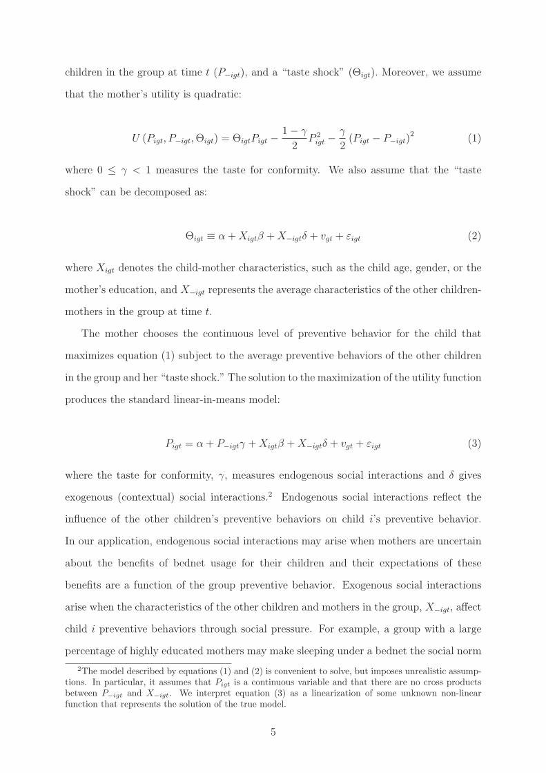
children in the group at time t (P−igt), and a “taste shock” (Θigt). Moreover, we assume

that the mother’s utility is quadratic:

U (Pigt, P−igt,Θigt) = ΘigtPigt −1− γ

2P 2igt −

γ

2(Pigt − P−igt)

2 (1)

where 0 ≤ γ < 1 measures the taste for conformity. We also assume that the “taste

shock” can be decomposed as:

Θigt ≡ α +Xigtβ +X−igtδ + vgt + εigt (2)

where Xigt denotes the child-mother characteristics, such as the child age, gender, or the

mother’s education, and X−igt represents the average characteristics of the other children-

mothers in the group at time t.

The mother chooses the continuous level of preventive behavior for the child that

maximizes equation (1) subject to the average preventive behaviors of the other children

in the group and her “taste shock.” The solution to the maximization of the utility function

produces the standard linear-in-means model:

Pigt = α + P−igtγ +Xigtβ +X−igtδ + vgt + εigt (3)

where the taste for conformity, γ, measures endogenous social interactions and δ gives

exogenous (contextual) social interactions.2 Endogenous social interactions reflect the

influence of the other children’s preventive behaviors on child i’s preventive behavior.

In our application, endogenous social interactions may arise when mothers are uncertain

about the benefits of bednet usage for their children and their expectations of these

benefits are a function of the group preventive behavior. Exogenous social interactions

arise when the characteristics of the other children and mothers in the group, X−igt, affect

child i preventive behaviors through social pressure. For example, a group with a large

percentage of highly educated mothers may make sleeping under a bednet the social norm

2The model described by equations (1) and (2) is convenient to solve, but imposes unrealistic assump-tions. In particular, it assumes that Pigt is a continuous variable and that there are no cross productsbetween P−igt and X−igt. We interpret equation (3) as a linearization of some unknown non-linearfunction that represents the solution of the true model.

5

for all children in the group.

We assume that vgt represents the group effect at time t that is observable to all

mothers in the group at time t, but unobervable to us. We allow vgt to be correlated with

Xigt and X−igt. Finally, εigt is the individual idiosyncratic component. We assume that

E (εigt|Xigt, X−igt, vgt) = 0 and that εigt is uncorrelated with εi′g′t′ for each i 6= i′ or g 6= g′

or t 6= t′.

Taking the expected value at the group-time level on both sides of equation (3) and

solving for P−igt leads to the social equilibrium for the group:

P−igt =α

1− γ+X−igt

(

β + δ

1− γ

)

+vgt

1− γ(4)

Substituting (4) into (3) and replacing X−igt with its sample counterpart Xgt =

1

mgt

∑

i

Xigt leads to the following individual-level equation:3

Pigt =α

1− γ+Xigtβ +Xgt

(

γβ + δ

1− γ

)

+vgt

1− γ+ ε∗igt (5)

where

ε∗igt = εigt +

(

γβ + δ

1− γ

)

(

X−igt −Xgt

)

Taking sample group-time averages in (3) and solving for P gt =1

mgt

∑

i Xigt leads to

the group-level equation:

P gt =α

1− γ+Xgt

(

β + δ

1− γ

)

+vgt

1− γ+ ε′gt (6)

where

ε′gt =γ(

P−igt − P gt

)

+ δ(

X−igt −Xgt

)

+ εgt

1− γ

Following Glaeser and Scheinkman (2001), Glaeser et al. (2003), Auld (2011), and

Canning et al. (2013), the social multiplier is the ratio of the effect of characteristic X

on preventive behaviors at the group level over its effect on preventive behaviors at the

3We only observe a sample mgt < ngt of individuals from each group g at time t. This creates ameasurement error for variables based on sample averages.

6

individual level. In other words, the social multiplier is the ratio of β+δ

1−γfrom equation (6)

and β from equation (5), that is:

Social Multiplier =

β+δ

1−γ

β

In the absence of social interactions (γ = 0 and δ = 0), the social multiplier equals

1 because the effect of any characteristic on preventive behaviors is the same at the

individual level and at the group level. In contrast, in the presence of endogenous social

interactions (0 < γ < 1) and assuming no exogenous social interactions (δ = 0), the

social multiplier equals 11−γ

and is thus greater than one. Symmetrically, when there is no

endogenous social interaction (γ = 0) and only exogenous social interactions (δ 6= 0), and

provided that β and δ have the same sign, the social multiplier is also greater than one.

Finally, when there are both endogenous and exogenous social interactions (0 < γ < 1

and δ 6= 0), and provided that β and δ have the same sign, the social multiplier is also

greater than one.

3. IDENTIFICATION AND ESTIMATION STRATEGY

This section is divided into four subsections. First, we define our reference group

and discuss the implications of this choice. Second, we present the contextual effects we

focus on in this study. Third, we examine the identification of the individual-level model.

Fourth, we discuss the identification of the regional-level model.

3.1. Reference Group

We define an individual’s reference group as all the individuals who live in the same

region, split into its urban and rural parts. This is the most precise level of disaggregation

we can use in our data, as the (split) region is the smallest geographical entity that we

can follow over time. The construction of the geographical regions is presented in details

in Section 4.

Note that all of our survey samples are collected from geographical clusters which

are smaller and more precise than regions. However, we do not use the cluster as our

7

reference group for two reasons. First, within any country, the clusters selected change

in each survey. It is therefore impossible to apply cluster fixed effects in our group-level

regressions. Second, the number of children under 5 and pregnant women within each

cluster is small, and so measurement error in calculating group averages would be large.

In this paper, we measure the social interactions that occur within (split) regions.

However, there might also be social interactions across urban and rural areas within the

same region, or across regions, or even across countries. We expect the social multiplier

to increase with the level of aggregation. As a consequence, we interpret our results on

the social multiplier within (split) regions as lower bounds.

In addition to larger geographical areas (the unsplit region, the country, a set of

countries), the reference group could also be defined by cultural traits such as ethnicity,

local dialect, or religion. In the future, researchers may be interested in investigating

social interactions using these alternative definitions of the group.

3.2. Explanatory Variables and Exogenous Social Interactions

Our models of bednet usage include the following list of explanatory variables: the

child’s age and gender, the mother’s age and education, household size, and household

wealth. In our analysis of preventive treatment during pregnancy, we control for the

woman’s age and education, household size, and household wealth.

When we examine the social multipliers, we focus on the mother or woman’s educa-

tion and on household wealth, because these variables can be influenced by governmental

policies on the one hand, and because they are likely to generate exogenous social inter-

actions on the other hand. We expect educated and wealthy women to be more likely to

use preventive methods (because they understand their benefits) and to be respected and

imitated by their neighbors. Consequently, we expect education and wealth to generate

exogenous social interactions, meaning that a woman’s decision regarding prevention will

be positively influenced by the average education and wealth level in her group.

8

3.3. Individual-Level Model

We use the individual-level model in equation (5) to identify the denominator of the

social multiplier, β. We estimate this equation including cluster fixed effects, which are

time variant. The inclusion of these cluster fixed effects perfectly control for unobserved

factors that affect malaria preventive behaviors for everyone in the cluster at time t

such as malaria campaigns, weather, and earning prospects. Unfortunately in equation

(5), the inclusion of cluster fixed effects captures any characteristic that is region-time

specific. Consequently, the inclusion of these fixed effects does not allow us to identify

the coefficients on Xgt.

3.4. Aggregate-Level Model

We use the aggregate-level equation (6) to identify the numerator of the social multi-

plier, β+δ

1−γ.

3.4.1. Main Model

In our main model, we decompose vgt into three effects: (i) a time-invariant group-

specific effect vg, (ii) a vector of country (c) specific time-variant controls Z1ct, and (iii) a

vector of region-specific time-variant controls Z2gt:4

P gt =α

1− γ+Xgt

(

β + δ

1− γ

)

+vg

1− γ

+θ1Z1ct

1− γ+

θ2Z2gt

1− γ+ ε′gt, (7)

vg controls for omitted factors that are time invariant and affect the malaria preventive

behaviors for everyone in the group (for instance, the level of malaria prevalence or the

ethnic composition of the group). Moreover, Z1ct controls for time-variant omitted factors

that affect the malaria preventive behaviors of everyone in the country. Z1ct includes a

survey (i.e. country-time) dummy and country-specific time trends and their squares. Fi-

nally, Z2gt captures omitted factors that affect high malaria prevalence regions differently,

4Controlling for region-time fixed effects is not an option because they are perfectly correlated withXgt.

9

and it controls for time-variant weather-related factors that affect the malaria preven-

tive behaviors of everyone in the region depending on whether the interview is conducted

during the rainy or malaria seasons. Specifically, Z2gt includes an interaction between

a time-invariant region-specific malaria ecology index and a time trend, an interaction

between the malaria ecology index and a time trend square, and the precipitation and

temperature deviations. The precipitation (or temperature) deviation equals the differ-

ence between the month of the interview precipitation (or temperature) in the region and

the annual average precipitation (or temperature) in the region. The precipitation and

temperature deviations are used in the analysis of bednet usage only.

Although the empirical model given in equation (7) controls for many potential omitted

factors that might be correlated with Xgt, it does not control for all possible region-time

variant factors that might cause an omitted variable bias. This could happen in two

situations in particular. First, it is possible that between surveys there are migrations

into a region within a country from people of different ethnic backgrounds. This is likely to

change the region aggregate levels of education, wealth, and malaria preventive behaviors.

Second, it is also possible that national authorities target regions with low education

and/or wealth for mass net or IPTp campaigns.5

In sum, in our main model, we estimate β in equation (5) under weaker assumptions

than β+δ

1−γin equation (7) because we control for cluster fixed effects in equation (5), but

we only control for survey fixed effects, region fixed effects, country-specific time trends,

trends that depend on the level of malaria ecology in the region, and precipitation and

temperature deviations in equation (7). To assess the importance of controlling for cluster

omitted variable biases, we also estimate equation (5) without cluster fixed effects and

including the same controls as in equation (7).

5We conducted research on the policies of many of the countries in our sample and found that netdistribution campaigns tend to be national, without targeting a particular region. For example, inMadagascar (with the exception of three districts in the Vakinankaratra province, which is dropped inour sample) campaigns have been offering ITNs free of charge across the whole country, starting in 2004(Snow et al., 2012), whereas in Benin, treated nets have continuously been distributed nation-wide forpregnant women and children after malaria was declared the most important disease for children under5 in 2007 (Damien et al., 2010).

10

3.4.2. Measurement Error and Split-Sample IV Model

Another potential source of bias when estimating equation (7) is measurement error

in the explanatory and dependent variables, since we use the sample averages instead of

the true population averages (ε′gt =(

γ(

P−igt − P gt

)

+ δ(

X−igt −Xgt

)

+ εgt)

/ (1− γ) in

equation (7)).

Measurement error in the explanatory variables is likely to lead to an attenuation bias

as in the classical error-in-variables model. Following Graham and Hahn (2005), Canning

et al. (2013), and Auld (2011), we correct for measurement error in the explanatory

variables using the split-sample IV method proposed by Angrist and Krueger (1995). In

this method, we randomly split the sample within each (split) region and year into two

subgroups 1 and 2, and we calculate the means of the characteristics for the subgroups,

X(1)gt and X(2)gt. Because of the random assignment into the subgroups, measurement

errors in X(2)gt are uncorrelated with measurement errors in X(1)gt. We can then use

X(2)gt as instruments for X(1)gt to get consistent estimates of the regional means.

Measurement error in the dependent variable may create a bias if women in regions

with high levels of education and wealth missreport/overstate their preventive behaviors

due to social pressure. We assume that the potential bias due to correlations between the

measurement error in the dependent variable and the explanatory variables is small and

can be ignored.

4. DATA

The data come from the Demographic and Health Surveys (DHS), Malaria Indicator

Surveys (MIS), AIDS Indicator Surveys (AIS), and Multiple Indicator Cluster Surveys

(MICS) for countries in Sub-Saharan Africa. These surveys are large and nationally

representative. DHS, MIS, and AIS are part of the MEASURE DHS project, which is

partially funded by USAID. The goal of the DHS project is to monitor the population and

health situations of the target countries. DHS/MIS/AIS data contain detailed information

on health and preventive health behaviors for children, women, and men. MICS is funded

by UNICEF and it is used to monitor the situation of children and women.

11

Starting in 1999-2000, DHS/MIS/AIS and MICS began collecting information on the

use of mosquito nets, whether the nets are ITNs, and intermittent preventive treatments

for past pregnancies (IPTp). Because malaria eradication was not a health policy priority

before the creation of the Roll Back Malaria Partnership, DHS/MIS/AIS and MICS do not

include questions related to malaria prevention before 1999-2000. Fortunately, DHS, MIS,

and AIS use the same basic malaria questions, making comparisons between and within

countries using these surveys straightforward. MICS questionnaires are not identical

to DHS/MIS/AIS, but comparable measures of malaria prevention between MICS and

DHS/MIS/AIS can still be obtained.

DHS/MIS/AIS/MICS samples are drawn from geographical clusters. These clusters

are obtained from the previous census enumeration areas (EAs) and they are nationally

representative. Clusters vary in size and population but typically contain around 500

individuals. In rural areas, a cluster is usually a village or group of villages, and in urban

areas, it is about a city block.

For each individual, the data contain information on his region of residence, his clus-

ter of residence, and whether his cluster is in a urban or rural setting. Our aggregate

geographical group is the region of residence split into rural and urban clusters. Thus, we

create two groups per region. One group is made of all urban clusters in the region and

the other group is composed of all rural clusters in the region.

For some countries, the boundaries of some regions have changed between surveys

conducted in different years. In these instances, we combine regions using maps provided

in the public report of each survey. We drop groups with less than 100 observations,

because small cells would lead to unreliable group estimates.

We restrict our data to countries for which we have at least two usable DHS/MIS/AIS/

MICS surveys containing comparable information on malaria prevention between 1999 and

2012. Table I describes our data. We use 92 surveys (mainly DHS and MICS) covering

29 countries. Malaria is endemic in all the countries we use in our analysis, according to

the Roll Back Malaria website.6 The number of surveys per country ranges from two (for

6See www.rollbackmalaria.org/endemiccountries.html

12

11 countries) to five (for Malawi, Nigeria, Rwanda, and Senegal).

[Insert Table I here]

We merge the DHS/MIS/AIS/MICS regions with monthly precipitation and temper-

ature data from 1999 to 2012 based on weather station observations and interpolations

from the Climatic Research Unit (CRU), available at www.cru.uea.ac.uk.

We also merge the DHS/MIS/AIS/MICS regions with a measure of malaria prevalence

(PfPR2−10) for 2010 obtained from the Malaria Atlas Project (MAP) databases which are

publicly available at www.map.ox.ac.uk. PfPR2−10 captures the percentage of children

ages 2 to 10 who have detectable levels of the Plasmodium falciparum parasite in their

peripheral blood. PfPR2−10 is constructed from parasite surveys that are periodically

carried out in areas known to have malaria. Then, using Bayesian geostatistical algorithms

with adjustments for climatic and environmental factors, MAP made projections in time

and space to create a continuous display of PfPR2−10, called the Malaria Endemicity

map, for all of Africa in 2010. Gething et al. (2011) provide details on the construction

of PfPR2−10.

5. EMPIRICAL SPECIFICATION

Overview: We estimate equations (5) and (7) separately for children under 5 and

for women who gave birth over the two years preceding the interview. When estimat-

ing equation (5), we use individual-level variables, whereas for equation (7), we use the

averages of the variables in the group.7

We do not use sample weights because when the model is correctly specified, ordinary

least squares results are consistent (Deaton, 1997; Solon et al., 2013). In addition, weights

should be based on the population in each region and survey, but we do not have the true

populations for all regions and surveys in our data.

Dependent Variables: For children under 5, we study the following dependent

variables: (i) whether the child slept under any type of mosquito net the night before

7An overview of the variables is given in Appendix A.

13

the survey, and (ii) whether the child slept under an ITN the night before the survey.

Sleeping under an ITN is considered to be the main tool to fight malaria in the RBM

partnership arsenal.

For women who gave birth over the two years preceding the interview, we use the

following dependent variables: (i) whether the woman took at least one dose of Fansidar

during her last pregnancy, and (ii) whether the woman took at least two doses on Fansi-

dar during her last pregnancy. WHO recommendation is that women take two doses of

Fansidar. In that case, it is considered that they complete the IPTp treatment.

Explanatory Variables: In the children models, we control for the mother’s edu-

cation, household wealth, child age, whether the child is a male, the mother’s age, and

household size. In the women analysis, we include controls for the woman’s education,

household wealth, the woman’s age, and household size. The mother or woman’s ed-

ucation is a binary indicating whether the mother or woman has secondary education

or higher. The wealth variable is a dummy for whether the household has an improved

source of drinking water or improved sanitation facilities.8

Our specifications also include controls for cluster fixed effects (equation (5)), survey

fixed effects (equation (7)), region fixed effects (equation (7)), country-specific trends

(equation (7)), trends interacted with malaria ecology (equation (7)), and precipitation

and temperature deviations (equation (7), children sample).

The malaria ecology index captures the variation in malaria prevalence in the region

that is explained by climatic factors. We construct the malaria ecology index using

PfPR2−10 for 2010, the average precipitation and temperature data, the average maximum

precipitation and temperature, and the average minimum precipitation and temperature.

The average precipitation (temperature) is the mean precipitation (temperature) between

2000 and 2010. To quantify the average maximum precipitation (temperature), we find

the month with the highest average precipitation (temperature) in the region for each

year and then average over all the years. Using the same procedure, we find the average

8The DHS/MIS/AIS contain an index of wealth reported in quintiles. This index is calculated basedon questions related to the possession of assets such as a radio or a bicycle. We do not use this measure,because it is not comparable across surveys.

14

minimum precipitation (temperature). We then take the squares, cubes, and quartics of

each of the six climate variables, leaving us with 24 climate variables.

We then regress malaria prevalence (PfPR2−10 in 2010) on our 24 climate variables.

The fit of the resulting prediction, with an R2 of 0.63, is very high (see Appendix B). Our

malaria ecology index is the prediction of malaria prevalence from this regression.

When estimating equation (7) for the children sample, we control for precipitation and

temperature deviations. The precipitation (respectively temperature) deviation variable

captures the difference between the month of the interview precipitation (temperature)

and the annual average precipitation (temperature) in the region. These deviations are

calculated as follows. We begin by taking the level of precipitation (temperature) for each

region in each month from 1999 to 2012. We then take the average over the 12 months

preceding the interview to get the annual average precipitation (temperature) for a region.

The deviation is just the month of the interview precipitation (temperature) minus the

annual average precipitation (temperature) for each region.

6. MAIN RESULTS

6.1. Descriptive Statistics

Descriptive statistics are reported in Table II. In column (1), we show the descriptive

statistics for the individual-level data, whereas in columns (2) to (4), we present the

descriptives for the regional-level data. While column (2) contains the descriptives for the

whole period 1999-2012, columns (3) and (4) present them for the sub-periods 1999-2005

and 2006-2012.

Column (1) shows that only 29% of children under 5 slept under a bednet the night

before the survey and only 21% slept under an ITN. The percentage of women who took

at least one dose of Fansidar is 34%, but the percentage who took at least two doses of

Fansidar is only 18%. The mean child age is 2 years and the mean mother or women’s

age is around 27 years. Only 13-15% of mothers or women have secondary education and

the average household size is approximately 8 members.

15

Column (2) contains the regional-level statistics for 1999-2012. Note that as expected

the means at the regional level in column (2) are different from the means at the individual

level in column (1). However, the differences between columns (1) and (2) are generally

small, because the regions are rather homogenous, implying that the means of the variables

are rather similar across regions. By contrast, for women’s preventive behaviors, the

means in column (2) are different from those in column (1): this is due to the heterogeneity

in preventive treatment between regions (with some regions where preventive treatment

is common and others where it is rare), and to the fact that regions have different sample

sizes.

When we break up the 1999-2012 period into two sub-periods, 1999-2005 in column

(3) and 2006-2012 in column (4), we see that the regional means of all four preventive

behaviors increase over time, but the increase is substantially stronger for sleeping under

an ITN and taking two doses of Fansidar. Similarly, among the explanatory variables,

the share of educated mothers and of wealthy households also improve over time.

The sample size for the individual-level models varies from 88,316 observations for

taking two doses of Fansidar to 662,105 observations for sleeping under any type of bednet.

For the regional-level regressions, the sample size ranges from 356 to 1,436 observations.

[Insert Table II here]

6.2. Main Model

Table III displays the regression results of our main model, for sleeping under any

type of bednet in Panel A and for sleeping under an ITN in Panel B. Columns (1) to (3)

give the results of the individual-level regressions, whereas column (4) gives the results of

the regional-level regression. Column (1) presents the results without controlling for any

fixed effect, column (2) controls for the exact same fixed effects as in the regional-level

model in column (4), and column (3) controls for cluster fixed effects.

[Insert Table III here]

In both Panels A and B, the coefficients on children’s and women’s demographics in

column (1) are somewhat different from those in models that do control for fixed effects

16

in columns (2) and (3). This highlights that adequately controlling for unobserved factors

is necessary for our study. As a consequence, we will not comment on the results from

column (1).

In Panel A, individual models in columns (2) and (3) show that the mother’s secondary

education increases the probability that the child sleeps under any type of bednet by 6.7

and 5.6 percentage points. In the regional model in column (4), the coefficient on the

mother’s secondary education is larger than in individual-level models, since maternal

education increases the probability that the child sleeps under any type of bednet by 12.7

percentage points. Moreover, individual-level models in columns (2) to (3) show that

household wealth increases the probability that the child sleeps under any type of bednet

by 3.2 and 2.2 percentage points. Again, the effect of wealth in the regional-level model

is greater, since wealth increases the probability that the child sleeps under any type of

bednet by 4.4 percentage points. However, the coefficient on wealth is not significant.

In Panel B, we find that the coefficient on the mother’s education is greater in the

regional-level model in column (4) than in the individual-level models in columns (2) and

(3). However, the coefficients on education and wealth are not significant in the regional-

level model. Our specification includes country-specific time trends that together with

(split) region fixed effects explain most of the variation in ITN usage at the group level.

All models indicate that sleeping under any type of bednet or under an ITN does not

depend on the child gender, since the coefficient for the child being a male is generally

small and is never significant. The effect of household size on bednet and ITN usage is

negative in our models, but the coefficient is significant in individual-level models only.

This finding is consistent with competition for resources within households: for a given

number of bednets and ITNs within a household, the likelihood that a bednet is allocated

to a child decreases with the number of household members.

Table IV reports the estimates for the preventive outcomes for women. Panel A con-

tains the results for taking at least one dose of Fansidar, whereas Panel B reports the

coefficients for taking two doses of Fansidar, which corresponds to the WHO recommen-

dation for pregnant women.

17

[Insert Table IV here]

In Panel A, specifications in columns (2) to (4) indicate that women with secondary

education are significantly more likely to adopt preventive behaviors than women with

no education or primary education only. This is an expected result, since women with a

higher education are more likely to be aware of the benefits of antimalarial drugs. We

also find that the coefficient on education in the regional-level regression in column (4)

is much larger than the coefficient in individual-level regressions in columns (2) and (3).

Similarly, the coefficient on household wealth is positive, significant, and greater in the

regional-level model than in the individual-level models. Results in Panel B are consistent

with those in Panel A, but the coefficients on education and wealth in the regional-level

models are not significant.

In both Tables III and IV, the estimated parameters in columns (2) and (3) are rather

similar, but they are different from the parameters in column (1). This suggests that our

decomposition of the unmeasured group effect, vgt (into survey fixed effects, region fixed

effects, different time trends, and precipitation and temperature deviations) is sufficient

to control for the omitted variable bias.

The social multipliers associated with education and wealth are reported in Table V.

[Insert Table V here]

The social multipliers for the mother’s or woman’s secondary education are com-

puted by dividing the coefficients on the mother’s or woman’s secondary education from

the regional-level regression in Tables III and IV, column (4), by the coefficients on the

mother’s or woman’s secondary education from the individual-level regressions, in Tables

III and IV, column (3). We use the same procedure to calculate the social multipliers

for wealth. We use bootstrap methods to calculate the 95% confidence intervals of the

social multipliers (Li and Maddala, 1999): 1,000 bootstrap samples are taken with ran-

domization at the country and regional level respectively (to maintain the panel structure

of the data). Note that the 95% confidence intervals of the multipliers are not symmetric;

symmetry of the confidence interval for a ratio only occurs in very large samples.

18

The social multipliers for education and wealth are significantly greater than one for

sleeping under any type of bednet, taking one dose of Fansidar or more, and taking two

doses of Fansidar or more. This suggests that the decision to adopt preventive behaviors

does not only depend on women’s education or household wealth, but also on the average

women’s education and household wealth in the region, and that there are spillovers

between households.

In addition, while the multipliers associated with sleeping under any type of bednet

are rather modest, those for antimalarial treatments during pregnancy are large. At first

sight, these large multipliers may seem implausible. However, the large social multipliers

for women’s preventive behaviors could also really capture the existence of strong social

interactions. In particular, that social interactions matter more for women’s treatment

uptake than for children’s bednet usage makes sense, since getting preventive treatment is

a public/social activity, whereas using a bednet is more private. It is easier for a woman

to observe her neighbor going to a health facility to get preventive treatment, than to

observe her neighbors’ child using a bednet at night. As a consequence, knowledge about

the neighbors’ preventive treatment uptake is more widespread, which should increase the

level of social interactions.

For sleeping under an ITN, we do not find that the social multipliers of education and

wealth are significantly greater than one. It is not clear whether this result reflects an

absence of social interactions for ITN usage or a lack of statistical power in the regional-

level model due to the lack of variation in our variables once we control for region fixed

effects and several time trends.

6.3. Split-Sample IV Model

Tables VI reports the results of the split-sample IV method that corrects for measure-

ment error in education and wealth in the regional-level model (see Section 3.4.2).

Column (1) contains the estimates from the regional-level model estimated with OLS

(from Tables III and IV), whereas column (2) reports the estimates when using SSIV.

For all four dependent variables, the first-stage F-statistics and Kleibergen-Paap Wald F-

statistics are large and we can reject the null hypothesis that the model is not identified.

19

The coefficients from the SSIV model are rather similar to the ones from the OLS model,

which suggests that measurement error is small in our study and can be ignored.

[Insert Table VI here]

7. ROBUSTNESS CHECKS AND ADDITIONAL RESULTS

7.1. GMM/IV Model

We here relax the assumption that survey fixed effects, region fixed effects, country-

specific time trends, malaria ecology interacted with time trends, and precipitation and

temperature deviations completely address the endogeneity of Xgt in equation (7). Our

strategy is to take the first difference in equation (7) and then use lagged values of Xgt

as instruments, in a GMM/IV framework. Unfortunately, these intruments are weak and

most of the coefficients are unreliable. The method and results are presented in Appendix

C.

7.2. Controlling for Wealth Inequality

We re-estimate our models controlling for wealth inequality. We proxy wealth inequal-

ity with the standard deviation of wealth within the region for the year of the interview.

The results are reported in the online Appendix D, Table D.I. Note that we control for

wealth inequality in regional-level models, but not in individual-level models, because in

individual-level models, cluster fixed effects already capture the impact of any variable

that is fixed for any region-year.

In Table D.I, the individual-level estimates are thus the same as in Tables III and

IV. In Panels A, C and D, the regional-level coefficients on education and wealth are

generally comparable to those in Tables III and IV and they are greater than individual-

level coefficients (note that in the regional-level model, the coefficient on household wealth

for one dose of Fansidar or more is no longer significant though). Consequently, the social

20

multipliers on education and wealth will remain greater than one for sleeping under any

type of bednet and taking one or two doses of Fansidar or more.9

7.3. East and West Africa

We also consider differences in social interactions between East and West Africa. We

cannot detect any heterogeneity because of a lack of statistical power. The results of this

analysis are reported in the online Appendix E.

7.4. Excess Variance Across Groups

We finally check the robustness of our findings on the presence of social interactions in

malaria preventive behaviors by analyzing whether there is excess variance of preventive

behaviors across groups. Glaeser, Sacerdote, and Scheinkman (1996) and Graham (2008)

show that we can measure social interactions based on covariance restrictions of the dis-

turbances. In particular, social interactions create excess variance across groups and these

variances depend on the group size. Graham (2008) show that under the assumption of

random assignment for the linear-in-means model, we can identify social interactions by

using differences in the variance of outcomes of groups of different sizes. Unfortunately,

we do not have information on the group sizes (e.g. the population of the split regions)

and we cannot implement this method.

Our approach follows Auld (2011) and is based on comparing the actual estimated

standard deviation of our outcome across groups:

SPgroup=

√

√

√

√

1

#group

#group∑

gt=1

(

P gt − P)2

where P = 1N

∑N

i=1 Pigt and P gt =1

Ngt

∑Ngt

i=1 Pigt; with the estimated standard deviation

assuming that Pigt is i.i.d. with the same mean and standard deviation as in the actual

data. If social interactions are present under the assumption of random assignment and

9Note that other factors, such as the perception of the value of life, may have an impact on the decisionto adopt preventive behaviors against malaria. Our data do not contain information on such perceptionsthough. If we assume that the perception of the value of life is the same for all individuals in any cluster,then our individual-level models with cluster fixed effects already control for the perception of the valueof life. However, this might be a strong assumption. We leave this point for future research.

21

no unmeasured group effects, the group standard deviation using actual data will be larger

than the group standard deviation using counterfactual data.

We consider two different group definitions: 1) cluster-time combinations of individu-

als, and 2) region-time combinations of individuals.

Because many differences in the group variances are caused by individual and group

characteristics, we repeat the analysis but in a first stage we regress Pigt on individual

characteristics, time trends and region fixed effects, and we then use the residuals to

calculate the standard deviations.

In Appendix F, Table F.I, Panel A shows the results for the standard deviations based

on the raw data. We find that there is an excess variance at the group level that becomes

larger with the size of the group. In Panel B, we control for individual characteristics,

time trends, and region fixed effects, and still find excess variance at the group level. We

need to be cautious when interpreting these results because this method does not control

for unmeasured heterogeneity across groups. However, the results are consistent with the

existence of social interactions.

8. CONCLUSION

If the Millennium Development Goal of the United Nations of eliminating all avoidable

deaths caused by malaria is to be achieved, the level of malaria prevention must not only

increase substantially from current levels, but must also remain high and become the new

social norm. This paper examines whether there is a social multiplier in the adoption of

mosquito nets by children and preventive treatment during pregnancy by women. This

social multiplier can be caused by either endogenous social interactions, exogenous social

interactions, or both. In this paper, although we cannot examine the source of social

interactions, we can identify their existence by quantifying the social multiplier. As far

as we are aware, we are the first to investigate this topic.

Our results are consistent with the possibility of large social multipliers associated with

education and wealth for antimalarial drugs take up during pregnancy and more modest

social multipliers for bednet usage. These results are plausible. In Africa, antimalarial

22

drugs during pregnancy are administered during visits to antenatal clinics. Everyone in a

particular neighborhood can observe if a woman is pregnant and whether she attends the

antenatal clinic as scheduled. In contrast, sleeping under a bednet is not easily observable

for individuals outside the household. Thus, peer pressure and the opportunities for social

interactions are likely to be larger for antimalarial drugs during pregnancy compared to

bednet usage.

The existence of social multipliers suggests that the steady state or long-run effect of

a policy that increases the use of bednets or antimalarial treatments during pregnancy

(promotional campaigns or subsidies of bednets and treatments) will be larger than what

we would have predicted using the individual-level coefficients, once all the indirect effects

caused by social interactions are accounted for. Moreover, when combined with invest-

ments in education and infrastructure, these policies will generate large multiplier effects.

Thus, the cost of achieving the Millennium Goals will be smaller than in the absence of

spillovers.

23

ACKNOWLEDGEMENTS

The authors thank the editor Owen O’Donnell, two anonymous referees, ChristopherAuld, Kofi Awusabo-Asare, Anirban Basu, Luc Behaghel, Massimiliano Bratti, Pasca-line Dupas, Stacey Gelsheimer, Pierre-Yves Geoffard, Laurent Gobillon, Andrew Jones,Lahiri Kajal, Robyn Kibler, Jose Carlos A. Kimou, Sebastian Linnemayr, Carine Milcent,Drah Hannah Owusua, Thomas Piketty, Gregory Ponthiere, Bastian Ravesteijn, SilvanaRobone, Pedro Rosa Dias, Nicole Schoenecker, Tom Van Ourti, Atheendar Venkatara-mani, Bruno Ventelou, Joshua Wilde, Arseniy Yashkin, participants at the conferences“Economics of Disease” (2013) and Journees Louis-Andre Gerard-Varet (2013), a sem-inar in Paris School of Economics (2013), the Congress of the European Economic As-sociation (2013), the Twenty Second European Workshop on Econometrics and HealthEconomics (2013), and especially Michael Darden, for useful comments. Research assis-tance of Stacey Gelsheimer, Robyn Kibler, and Arseniy Yashkin was greatly appreciated.This paper was partially written while Benedicte Apouey was an Assistant Professor inEconomics at the University of South Florida. The authors thank the support of GrantNumber R03TW009108 from Fogarty International Center. The content is solely respon-sibility of the authors and does not necessarily represent the official views of the FogartyInternational Center or the National Institute of Health.

24

REFERENCES

Angrist J, Krueger A, 1995. Split-sample instrumental variable estimates of the returnto schooling. Journal of Business and Economic Statistics 13: 225-235.

Auld MC, 2011. Effect of large-scale social interactions on body weight. Journal of

Health Economics 30: 303-316.

Bernheim BD, 1994. A theory of conformity. Journal of Political Economy 102: 841-877.

Binka FN, Kubaje A, Adjuik M, Williams LA, Lengeler C, Maude GH, Armah GE, Kaji-hara B, Adiamah JH, Smith PG, 1996. Impact of permethrin impregnated bednetson child mortality in Kassena-Nankana district, Ghana: a randomized controlledtrial. Tropical Medicine and International Health 1: 147-154.

Blume LE, Brock WA, Durlauf SN, Jayaraman R, 2011. Linear Social Network Models.Unpublished manuscript. Available athttp://www.econ.cam.ac.uk/conf/networks-docs/bbdj08-19-11.pdf

Canning D, Gunther I, Linnemayr S, Bloom D, 2013. Fertility choice, mortality expec-tations and interdependent preferences. European Economic Review 63: 273-289.

Cohen J, Dupas P, 2010. Free distribution or cost-sharing? Evidence from a randomizedmalaria prevention experiment. Quarterly Journal of Economics CXXV: 1-45.

Conley T, Udry C, 2010. Learning about a new technology: pineapple in Ghana. Amer-

ican Economic Review 100: 35-69.

Damien GB, Djenontin A, Rogier C, Corbel V, Bangana SB, Chandre F, Akogbeto M,Kinde-Gazard D, Massougbodji A, Henry M-C, 2010. Malaria infection and diseasein an area with pyrethroid-resistant vectors in southern Benin. Malaria Journal 9:380.

Deaton A, 1997. The Analysis of Household Surveys. Baltimore: Johns Hopkins Uni-versity Press.

Dupas P, 2009. What matters (and what does not) in households’ decision to invest inmalaria prevention? American Economic Review 99: 224-230.

Ellison G, Fudenberg D, 1993. Rules of thumb for social learning. Journal of Political

Economy 101: 612-643.

Gething PW, Patil AP, Smith DL, Guerra CA, Elyazar IR, Johnston GL, Tatem AJ,Hay SI, 2011. A new world malaria map: Plasmodium falciparum endemicity in2010. Malaria Journal 10: 1475-2875.

Glaeser E, Sacerdote B, Scheinkman JA, 1996. Crime and social interactions. QuarterlyJournal of Economics CXI: 507-548.

25

Glaeser EL, Sacerdote BI, Scheinkman JA, 2003. The social multiplier. Journal of the

European Economic Association 1: 345-353.

Glaeser E, Scheinkman JA. Non-market interactions. Advances in economics and econo-metrics: theory and applications. Eighth World Congress of the Econometric Soci-ety. 2002.

Goodman CA, Mills AJ, 1999. The evidence base on the cost-effectiveness of malariacontrol, measures in Africa. Health Policy and Planning 14: 301-312.

Graham BS, 2008. Identifying social interactions through conditional variance restric-tions. Econometrica 76: 643-660.

Graham BS, Hahn J, 2005. Identification and estimation of the linear-in-means modelof social interactions. Economics Letters 88: 1-6.

Lengeler C, 2004. Insecticide-treated bed nets and curtains for preventing malaria.Cochrane Database of Systematic Reviews 2.

Li H, Maddala GS, 1999. Bootstrap variance estimation of nonlinear functions of param-eters: an application to long-run elasticities of energy demand. Review of Economics

and Statistics 81: 728-733.

Malaria Atlas Project (MAP). Available from www.map.ox.ac.uk.

Manski CF, 1993. Identification of endogenous social effects: the reflection problem.Review of Economic Studies 60: 531-542.

Picone G, Kibler R, Apouey B, 2013. Malaria prevalence, indoor residual spraying, andinsecticide-treated net usage in Sub-Saharan Africa. Working paper series, ParisSchool of Economics, No. 2013-40.

Solon G, Hayder, Wooldridge J, 2013. What are we weighting for? Working paper,Michigan State University.

Roll Back Malaria (RBM) Partnership 2010. World Malaria Day 2010: Africa Update.RBM Progress and Impact Series. No 2.

Snow RW, Amratia P, Kabaria CW, Noor AM, Marsh K, 2012. The changing limits andincidence of malaria in Africa: 1939-2009. Advances in Parasitology 78: 169-262.

Wiseman V, Hawley WA, Ter Kuile FO, Phillips-Howard PA, Vulule JM, Nahlen BL,Mills AJ, 2003. The cost-effectiveness of permethrin-treated bednets in an areaof intense malaria transmission in western Kenya. American Journal of Tropical

Medicine and Hygiene 68: 61-67.

World Health Organization (WHO) 2012 – World Malaria Report. Available athttp://www.who.int/malaria/publications/world malaria report 2012/en/index.html

26

Table I. Data sources

No. No.Country waves regions SurveysAngola 3 17 MICS01, MIS06, MIS11Benin 2 6 DHS01, DHS06Burkina Faso 3 13 DHS03, MICS06, DHS10Burundi 4 17 MICS00, MICS05, DHS10, DHS12Cameroon 4 12 MICS00, DHS04, MICS06, DHS11Central African Republic 2 17 MICS00, MICS06Chad 2 8 MICS01, DHS04Cote d’Ivoire 4 11 MICS00, AIS05, MICS06, DHS11Democratic Republic of the Congo 3 11 MICS01, DHS07, MICS10Gambia 2 8 MICS00, MICS05Ghana 3 10 DHS03, MICS06, DHS08Kenya 2 8 DHS03, DHS08Liberia 2 15 MIS08, MIS11Madagascar 4 6 MICS00, DHS03, DHS08, MIS11Malawi 5 26 DHS00, DHS04, MICS06, DHS10, MIS12Mali 2 9 DHS01, DHS06Mozambique 2 10 DHS03, DHS11Namibia 2 12 DHS00, DHS06Niger 2 8 MICS00, DHS06Nigeria 5 36 DHS03, MICS07, DHS08, MIS10, MICS11Rwanda 5 12 DHS00, MICS00, DHS05, DHS(I)07, DHS10Senegal 5 10 MICS00, DHS05, MIS06, MIS08, DHS10Sierra Leone 4 4 MIC00, MICS05, DHS08, MICS10Swaziland 3 4 MICS99, DHS06, MICS10Tanzania 4 21 DHS04, AIS07, DHS09, AIS11Togo 3 6 MICS00, MICS06, MICS10Uganda 4 4 DHS00, DHS06, MIS09, DHS11Zambia 3 9 MICS00, DHS01, DHS07Zimbabwe 3 10 DHS99, DHS05, DHS10

Total 92 surveys 340∗

Notes. AIS stands for AIDS Indicator Survey, DHS for standard Demographic and Health Survey, DHS(I)for interim DHS, MICS for Multiple Indicator Cluster Survey, and MIS for Malaria Indicator Survey.∗Each region will be divided in two (one rural, one urban) in the rest of the analysis and the regions with

less than 100 observations will be dropped.

27

Table II. Summary statistics

Individual level Regional level Regional level1999-2012 1999-2012 1999-2005 2006-2012Mean Mean Mean Mean(Std) (Std) (Std) (Std)

Children’s preventive outcomes

Sleeping under any type of bednet 0.296 0.289 0.192 0.349(0.456) (0.229) (0.196) (0.228)

Sleeping under an ITN 0.215 0.209 0.051 0.299(0.411) (0.221) (0.074) (0.226)

Women’s preventive outcomes

One dose of Fansidar or more 0.349 0.379 0.227 0.471(0.476) (0.329) (0.290) (0.312)

Two doses of Fansidar or more 0.187 0.199 0.071 0.290(0.390) (0.215) (0.132) (0.216)

Children’s demographics

Mother’s secondary education 0.151 0.179 0.142 0.202(0.358) (0.179) (0.165) (0.207)

Household wealth 0.658 0.687 0.633 0.720(0.474) (0.240) (0.246) (0.230)

Child age 1.954 1.954 1.930 1.968(1.419) (0.108) (0.103) (0.109)

Child is male 0.502 0.502 0.500 0.503(0.499) (0.030) (0.031) (0.030)

Mother’s age 26.996 27.055 27.676 26.668(10.753) (2.674) (2.199) (2.866)

Household size 7.740 7.549 7.736 7.432(4.821) (2.369) (2.269) (2.424)

Women’s demographics

Secondary education 0.134 0.154 0.154 0.158(0.341) (0.190) (0.192) (0.188)


Age 27.551 27.588 27.457 28.109(6.852) (1.238) (1.373) (1.050)

Household size 7.814 7.746 7.324 7.872(5.296) (3.029) (2.612) (3.129)

Obs. for Sleeping under any type of bednet 662,105 1,436 - -Obs. for Sleeping under an ITN 601,031 1,342 - -Obs. for One dose of Fansidar or more 95,555 388 - -Obs. for Two doses of Fansidar or more 88,316 356 - -

28

Table III. Regressions for preventive behaviors for children (OLS)

Individual Individual Individual RegionalEquation (5) Equation (5) Equation (5) Equation (7)

OLS OLS OLS OLS(1) (2) (3) (4)

Panel A. Dependent variable: Sleeping under any type of bednet

Mother’s secondary education 0.0265** 0.0676*** 0.0563*** 0.127**(0.0131) (0.0016) (0.0042) (0.0609)

Household wealth 0.0403*** 0.0328*** 0.0226*** 0.0446(0.0117) (0.0012) (0.0021) (0.0334)

Age (/10) -0.138*** -0.153*** -0.154*** 0.0828(0.0070) (0.0036) (0.0055) (0.414)

Male -0.0005 -0.0015 -0.0013 -0.0274(0.0010) (0.0009) (0.0009) (0.115)

Mother’s age (/10) -0.0066*** 0.0026*** 0.0036*** -0.0034(0.0021) (0.0007) (0.0009) (0.0565)

Household size -0.0040*** -0.0057*** -0.0062*** -0.0012(0.0011) (0.0001) (0.0003) (0.0039)

Malaria ecology * Time trend 0.0642*** 0.0789*(0.0084) (0.0467)

Malaria ecology * Time trend2 -0.0037*** -0.0053*(0.0005) (0.0030)

Precipitation (deviation) (/100) -0.0048*** 0.0024(0.0008) (0.0054)

Temperature (deviation) -0.0068*** -0.0061***(0.0003) (0.0021)

Observations 662,105 662,105 662,105 1,436R-squared 0.009 0.222 0.385 0.754Number of (split) regions 472

Panel B. Dependent variable: Sleeping under an ITN

Mother’s secondary education 0.0189* 0.0533*** 0.0451*** 0.0810(0.0101) (0.0039) (0.00356) (0.0572)

Household wealth 0.0391*** 0.0277*** 0.0179*** 0.0095(0.0113) (0.0023) (0.0021) (0.0327)

Age (/10) -0.106*** -0.120*** -0.122*** 0.144(0.0071) (0.0053) (0.0053) (0.417)

Male 0.0006 -0.0003 -0.0003 0.0345(0.0010) (0.0008) (0.0008) (0.113)

Mother’s age (/10) -0.0021 0.0026*** 0.0033*** -0.0255(0.0020) (0.0009) (0.0009) (0.0543)

Household size -0.0041*** -0.0044*** -0.0047*** -0.0048(0.0010) (0.0003) (0.0003) (0.0041)

Malaria ecology * Time trend 0.0454 0.0750*(0.0348) (0.0401)

Malaria ecology * Time trend2 -0.0019 -0.0046(0.0025) (0.0029)

Precipitation (deviation) (/100) -0.0077** -0.0124**(0.0030) (0.0054)

Temperature (deviation) -0.0010 -0.0030(0.0017) (0.0024)

Observations 601,031 601,031 601,031 1,342R-squared 0.007 0.260 0.396 0.815Number of (split) regions 430

Average Xs YesRegion FE Yes YesTime trend Yes YesTime trend2 Yes YesCountry FE × Time trend Yes YesCountry FE × Time trend2 Yes YesSurvey type FE Yes YesCluster FE Yes

Notes. The precipitation and temperature variables are the deviations from the monthy precipitation and temperatureaverages.“Average Xs” include average child age, the proportion of male children, average mother’s secondary education, mother’sage, household size, and wealth in the region.Robust standard errors, which are clustered by (split) region, are reported in parentheses.

*** denotes significance at 1% level. ** denotes significance at 5% level. * denotes significance at 10% level.29

Table IV. Regressions for preventive behaviors for women, for child deliveries in the lasttwo years (OLS)

Individual Individual Individual RegionalEquation (5) Equation (5) Equation (5) Equation (7)

OLS OLS OLS OLS(1) (2) (3) (4)

Panel A. Dependent variable: One dose of Fansidar or more

Secondary education -0.0156 0.0599*** 0.0507*** 0.469**(0.0263) (0.0066) (0.0067) (0.215)

Household wealth 0.0727*** 0.0306*** 0.0143*** 0.124*(0.0182) (0.0043) (0.0047) (0.0678)

Age (/10) -0.0168*** 0.0022 0.0021 -0.106(0.00524) (0.0017) (0.0019) (0.103)

Household size 0.0097*** 0.0003 0.0001 0.0086(0.0020) (0.0005) (0.0003) (0.0101)

Malaria ecology * Time trend -0.0213 0.0756(0.0696) (0.0784)

Malaria ecology * Time trend2 0.0021 -0.0042(0.0045) (0.0051)

Observations 95,555 95,555 95,555 388R-squared 0.017 0.454 0.580 0.901Number of (split) regions 146

Panel B. Dependent variable: Two doses of Fansidar or more

Secondary education -0.0024 0.0379*** 0.0334*** 0.206(0.0163) (0.0053) (0.0057) (0.206)

Household wealth 0.0441*** 0.0192*** 0.0081* 0.0851(0.0121) (0.0041) (0.0048) (0.0547)

Age (/10) -0.0127*** 0.0005 0.0006 -0.128*(0.0033) (0.0015) (0.0016) (0.0757)

Household size 0.0084*** -3.18e-05 -0.0001 0.0032(0.0013) (0.0003) (0.0002) (0.0076)

Malaria ecology * Time trend 0.0653 0.123**(0.0605) (0.0566)

Malaria ecology * Time trend2 -0.0033 -0.0070*(0.0040) (0.0037)

Observations 88,316 88,316 88,316 356R-squared 0.016 0.276 0.412 0.878Number of (split) regions 136

Average Xs YesRegion FE Yes YesTime trend Yes YesTime trend2 Yes YesCountry FE × Time trend Yes YesCountry FE × Time trend2 Yes YesSurvey type FE Yes YesCluster FE Yes

Notes. “Average Xs” include average age, secondary education, household size, and wealth in the region.Robust standard errors, which are clustered by (split) region, are reported in parentheses.

*** denotes significance at 1% level. ** denotes significance at 5% level. * denotes significance at 10% level.

30

Table V. Social multipliers

Sleeping Sleeping One dose Two dosesunder any type under of Fansidar of Fansidar

of bednet an ITN or more or moreMother’s or woman’s 2.364 1.715 9.243 6.161secondary education (0.449) (0.549) (2.229) (2.826)

[1.742, 3.353] [0.703, 2.793] [7.302, 14.435] [2.609, 16.369]


[1.273, 3.009] [-0.309, 1.710] [4.296, 18.791] [3.186, 49.365]

Notes. The multipliers are computed using the individual-level models that control forcluster fixed effects and the regional-level models. We bootstrap the standard errorsand confidence intervals of the social multipliers, applying a panel bootstrap using 1,000replications. The standard errors of the social multipliers are reported in paretheses. The95% bias-corrected confidence intervals of the social multipliers are reported in brackets.

31

Table VI. Regional-level regressions for preventive behaviors for children (OLS and split-sample IV)

Regional RegionalOLS SSIV(1) (2)


Mother’s secondary education 0.127** 0.1551**(0.0609) (0.0638)

Household wealth 0.0446 0.0403(0.0334) (0.0329)

Observations 1,436 1,436R-squared 0.754 0.882Number of (split) regions 472 472First stage F-stat for education [P-value] 650.31 [0.0000]First stage F-stat for wealth [P-value] 4920.48 [0.0000]Kleibergen-Paap Wald F-stat 199.61


Mother’s secondary education 0.0810 0.0748(0.0572) (0.0602 )


Observations 1,342 1,342R-squared 0.815 0.874Number of (split) regions 430 430First stage F-stat for education [P-value] 673.78 [0.0000]First stage F-stat for wealth [P-value] 3838.72 [0.0000]Kleibergen-Paap Wald F-stat 237.13

Panel C. Dependent variable: One dose of Fansidar or more

Secondary education 0.469** 0.5012**(0.215) (0.2363)

Household wealth 0.124* 0.1758*(0.0678) (0.0650)

Observations 388 388R-squared 0.901 0.959Number of (split) regions 146 146First stage F-stat for education [P-value] 68.32 [0.0000]First stage F-stat for wealth [P-value] 403.25 [0.0000]Kleibergen-Paap Wald F-stat 66.41

Panel D. Dependent variable: Two doses of Fansidar or more

Secondary education 0.206 0.2017(0.206) (0.1691)

Household wealth 0.0851 0.1014*(0.0547) (0.0546)

Observations 356 356R-squared 0.878 0.945Number of (split) regions 136 136First stage F-stat for education [P-value] 33.38 [0.0000]First stage F-stat for wealth [P-value] 558.47 [0.0000]Kleibergen-Paap Wald F-stat 33.63

Region FE Yes YesTime trend Yes YesTime trend2 Yes YesCountry FE × Time trend Yes YesCountry FE × Time trend2 Yes YesSurvey type FE Yes Yes

Notes. Split-sample estimates to correct for sampling error in education and wealth in regional models.Robust standard errors, which are clustered by (split) region, are reported in parentheses.


32

Online Appendix A

Table A.I. Variables used

DHS, MIS, MICS MICS MICSLabel AIS Wave 2 Wave 3 Wave 4Sleeping under any type of bednet hv228, v460, hml12 ml8 ml10 tn11Sleeping under an ITN hml12, hml19, ml0 ml9 ml12, ml13, ml14 tn5Taking Fansidar m49a Not available mn6* mn14aNo. of doses of Fansidar ml1 Not available mn6d mn16Child is male hv104, b4 hl3 hl4 hl4Child age hv105, b8 hl4 hl5 hl6Mother/Woman’s age hv105, v012 wi3b, memage, hl4, age wm9, hl5 wb2, hl6Mother/Woman’s education hc61, v106 melevel melevel melevelWater hv201 ws1 ws1 ws1Sanitation hv205 ws3 ws7 ws8Urban residence hv025 hi6 hh6 hh6Cluster hv001, v001 wiclno, chclno, hi1 hh1 hh1Region hv024, v024 hi7 hh7 hh7Year hv007, v007 hi3y hh5y hh5y

Notes. This table contains the “general” variables that we use in the analysis. Note that for some countries, we additionally

use country-specific variables. For many countries, the region variable is country-specific.

33

Online Appendix B

Table B.I. Regression to predict the malaria ecology index

PfPRCoeff. S.e.

Minimum precipitation -0.0140*** (0.0050)- square 0.0007* (0.0004)- cube -1.44e-05 (1.14e-05)- quartic 8.77e-08 (9.21e-08)Average precipitation 0.0139** (0.0058)- square -9.83e-05 (7.04e-05)- cube 4.66e-07 (3.67e-07)- quartic -8.20e-10 (6.86e-10)Maximum precipitation -0.0052** (0.0021)- square 3.02e-05*** (9.79e-06)- cube -7.15e-08*** (1.94e-08)- quartic 5.24e-11*** (0)Minimum temperature -0.123 (0.772)- square 0.0243 (0.0629)- cube -0.0013 (0.0022)- quartic 2.18e-05 (2.91e-05)Average temperature -21.63*** (4.707)- square 1.353*** (0.302)- cube -0.0373*** (0.0085)- quartic 0.0003*** (8.95e-05)Maximum temperature 12.25*** (2.884)- square -0.661*** (0.159)- cube 0.0158*** (0.0038)- quartic -0.0001*** (3.48e-05)Constant 43.50** (19.46)

Observations 399R-squared 0.636

Notes. In this table, the observation is the (unsplit) region. The table presents the results of the regressionof PfPR in the region on a number of precipitation and temperature variables in the same regino, in avery nonlinear setting. Our malaria ecology index is the linear prediction from this regression.Here the sample contains 399 (unsplit) regions. Note that this number of regions (399) is larger than thenumber of (unsplit) regions used in the rest of the paper (340 - See Table I). Indeed, here we use all theavailable countries from Sub-Saharan Africa, with information on PfPR, precipitation and temperature,to run the regression above and get a very general malaria ecology index. Some of the countries we usehere (Comoros, Equatorial Guinea, Guinea Bissau, Somalia, South Africa, and Sudan) do not have usableDHS/MIS/AIS/MICS data, and consequently cannot be used in the rest of the paper.Standard errors are reported in parentheses.

*** denotes significance at 1% level. ** denotes significance at 5% level. * denotes significance at 10%

level.

34

Online Appendix C

We here relax the assumption that survey fixed effects, region fixed effects, country-specific time trends, malaria ecology interacted with time trends, and precipitation andtemperature deviations completely address the endogeneity of Xgt in equation (7).

Assume that after controlling for all these variables, there is still a v∗gt that is correlated

with Xgt. Our strategy to address endogeneity takes the first difference of equation (7)and applies a GMM/IV estimator. Because different countries have surveys in differentyears, our first differences will not be with respect to the previous calendar year, but withrespect to the previous survey year which will be different by country. Specifically, ourtransformation is given by

P gtl,c − P gtl−1,c=

[

Xgtl,c −Xgtl−1,c

]

(

β + δ

1− γ

)

+θ1

(

Z1ctl,c − Z1ctl−1,c

)

1− γ+

θ2(

Z2gtl,c − Z2gtl−1,c

)

1− γ

+v∗gtl,c − v∗gtl−1,c

1− γ+(

ε′gtl,c − ε′gtl−1,c

)

This transformation eliminates the time-invariant component vg, but v∗gtl,c − v∗gtl−1,cwill

still be correlated with[


]

by definition. To obtain consistent estimates ofβ+δ

1−γ, we apply instrumental variables to this equation, using the lags Xgtl−2,c

as instru-

ments for[


]

. The main limitations of this approach is that it can only beimplemented for countries for which we have at least three waves of data and that thelags Xgtl−2,c

are likely to be a weak instrument for[


]

.Table C.I presents the results of the GMM/IV approach for children’s preventive

behaviors (in column (2)). The estimates are unreliable because of weak instruments (seethe low value of the first-stage F-statistics).

We do not provide the results of the GMM/IV method for women’s preventive behav-iors because the regional-level sample with three waves of data is too small.

35

Table C.I. Regional-level regressions (OLS and GMM/IV)

Regional RegionalOLS GMM/IV(1) (2)


Mother’s secondary education 0.127** -3.9056(0.0609) (22.8540)


Observations 1,436 492R-squared 0.754 -6.016Number of (split) regions 472 302First stage F-stat for education [P-value] 3.58 [0.0144]First stage F-stat for wealth [P-value] 1.21 [0.3057]Kleibergen-Paap Wald F-stat 0.0100


Mother’s secondary education 0.0810 -0.9385(0.0572) (3.9133)


Observations 1,342 482R-squared 0.815 -0.188Number of (split) regions 430 293First stage F-stat for education [P-value] 4.02 [0.0080]First stage F-stat for wealth [P-value] 1.17 [0.3216]Kleibergen-Paap Wald F-stat 0.04

Region FE Yes YesTime trend Yes YesTime trend2 Yes YesCountry FE × Time trend Yes YesCountry FE × Time trend2 Yes YesSurvey type FE Yes Yes

Notes. GMM/IV estimates to address the endogeneity of education and wealth in regionalmodels.Robust standard errors, which are clustered by (split) region, are reported in parentheses.

*** denotes significance at 1% level. ** denotes significance at 5% level. * denotes significance

at 10% level.

36

Online Appendix D

Table D.I. Models controlling for wealth inequality

Individual RegionalOLS OLS(1) (2)


Mother’s secondary education 0.0563*** 0.118*(0.0042) (0.0605)

Household wealth 0.0226*** 0.0365(0.0021) (0.0377)

S.d. of household wealth -0.0311(0.0561)

Observations 662,105 1,436R-squared 0.385 0.754Number of (split) regions 472


Mother’s secondary education 0.0451*** 0.0781(0.0035) (0.0571)



Observations 601,031 1,342R-squared 0.396 0.814Number of (split) regions 430


Mother’s secondary education 0.0507*** 0.445**(0.0067) (0.208)


S.d. of household wealth -0.187*(0.103)

Observations 95,555 388R-squared 0.580 0.903Number of (split) regions 146

Panel D. Dependent variabke: Two doses of Fansidar or more

Mother’s secondary education 0.0334*** 0.198(0.0057) (0.204)

Household wealth 0.0081* 0.0736(0.0048) (0.0558)


Observations 88,316 356R-squared 0.412 0.878Number of (split) regions 136

Cluster FE YesRegion FE YesTime trend Yes

Time trend2 YesCountry FE × Time trend Yes

Country FE × Time trend2 YesSurvey type FE Yes

Notes. The same controls as in Table III and IV are included.Robust standard errors, which are clustered by (split) region, are reported in parentheses.


37

Online Appendix E

Our analysis in Section 6 has investigated social interactions for Sub-Saharan Africaas a whole. However, one may expect differences in the level of social interactions betweenEast and West Africa, since West Africans are much more tribalists than East Africans,historically at least (we thank Michael Darden for this suggestion). To examine thatpoint, we break down our sample into Eastern and Western countries, and re-estimatethe individual- and regional-level models separately for the two samples. In our list ofcountries, the countries in West Africa are the following: Mali, Burkina Faso, Niger,Benin, Cote d’Ivoire, Gambia, Ghana, Liberia, Senegal, Sierra Leone, Togo, and Nige-ria, whereas the countries in East Africa are the following: Tanzania, Kenya, Uganda,Rwanda, Burundi, Ethiopia, Mozambique, Madagascar, Malawi, Zambia, and Zimbabwe.These list follow the United Nations scheme of geographic regions. Note that Angola,Cameroon, Central African Republic, Chad, and the Democratic Republic of the Congo,which are in Middle Africa according to the UN, are not separately analyzed because thenumber of observations is too small. Namibia and Swaziland, which are part of SouthernAfrica, are not analyzed either, because they also represent too few observations in oursample.

The results of the analysis are presented in Table E.I. Panels A and B report theresults for children’s preventive behaviors. The coefficients imply that for sleeping underany type of bednet, the social multiplier associated with the mother’s education is largerthan one in East Africa, whereas the social multiplier associated with household wealthis larger than one in West Africa. For sleeping under a treated net, the multiplier onhousehold wealth is also larger than one in West Africa.

Panels C and D contain the estimates for women’s preventive behaviors. For takingone dose of Fansidar or more, the social multiplier associated with education is greaterthan one in West Africa.

38

Table E.I. Main model for East and West Africa

Individual Regional Individual RegionalOLS OLS OLS OLS(1) (2) (3) (4)East Africa West Africa


Mother’s secondary education 0.0932*** 0.227** 0.0305*** -0.117(0.0073) (0.0966) (0.0040) (0.105)

Household wealth 0.0232*** 0.0012 0.0214*** 0.0838*(0.0032) (0.0599) (0.0033) (0.0474)

Observations 254,078 545 297,542 627R-squared 0.407 0.832 0.346 0.698Number of (split) regions 168 202


Mother’s secondary education 0.0760*** 0.116 0.0265*** -0.0402(0.0062) (0.0911) (0.0035) (0.110)

Household wealth 0.0196*** -0.0552 0.0169*** 0.0888*(0.0031) (0.0570) (0.0038) (0.0456)



Secondary education 0.0585*** 0.131 0.0300*** 0.972**(0.0084) (0.226) (0.0084) (0.442)

Household wealth 0.0105* 0.106 0.0212** 0.0952(0.0053) (0.112) (0.0084) (0.0753)


Panel D. Dependent variable: Two doses of Fansidar or more

Secondary education 0.0354*** 0.0220 0.0248** 0.503(0.0067) (0.216) (0.0119) (0.538)



Cluster FE Yes YesRegion FE Yes YesTime trend Yes YesTime trend2 Yes YesCountry FE × Time trend Yes YesCountry FE × Time trend2 Yes YesSurvey type FE Yes Yes

Notes. The same controls as in Table III and IV are included.Robust standard errors, which are clustered by (split) region, are reported in parentheses.


39

Online Appendix F

Table F.I. Excess variance across groups and social interactions

Standard deviation

Sleeping under Sleeping One dose Two dosesany type under of Fansidar of Fansidar

Group of bednet an ITN or more or morePanel A. Unadjusted standard deviations of malaria preventive behaviors

Individual 0.4582 0.4126 0.3862 0.4731

Cluster Actual 0.2886 0.2595 0.2404 0.3535Counterfactual 0.1230 0.1109 0.1454 0.1740Ratio 2.3463 2.3399 1.6534 2.0316

Region Actual 0.2322 0.2194 0.2108 0.3238Counterfactual 0.0270 0.0254 0.0254 0.0332Ratio 8.6000 8.6378 8.2992 9.7530

Panel B. Standard deviations of malaria preventive behaviors adjusted forobserved characteristics

Individual 0.4469 0.3876 0.3716 0.4516

Cluster Actual 0.2729 0.2233 0.2197 0.3298Counterfactual 0.1206 0.1038 0.1394 0.1643Ratio 2.2629 2.1513 1.5760 2.0073

Region Actual 0.1121 0.1118 0.2108 0.1717Counterfactual 0.0236 0.0214 0.0230 0.0238Ratio 4.7500 5.2243 9.1652 7.2143

Avg. cluster size 20.44 20.32 10.66 10.83Avg. region size 464.27 451.58 290.61 291.48

40

Social Interactions and Malaria Preventive Behaviors in ...

Documents

Transcript of Social Interactions and Malaria Preventive Behaviors in ...