ECONOMIC STUDIES

DEPARTMENT OF ECONOMICS SCHOOL OF BUSINESS, ECONOMICS AND LAW

GÖTEBORG UNIVERSITY 166

_______________________

Social Dilemmas: The Role of Incentives, Norms and Institutions

Marcela Ibáñez Díaz

ISBN 91-85169-25-0 ISBN 978-91-85169-25-2

ISSN 1651-4289 print ISSN 1651-4297 online

ECONOMIC STUDIES

DEPARTMENT OF ECONOMICS

SCHOOL OF BUSINESS, ECONOMICS AND LAW

GÖTEBORG UNIVERSITY

166

Social dilemmas:

The role of Incentives, Norms and Institutions.

Marcela Ibáñez Díaz

GÖTEBORG UNIVERSITY

2

A mi tía Inés y a mi Mamá

3

Abstract

The subject of this dissertation is social dilemmas. In a social dilemma situation, there

is a clear incentive not to cooperate. However, if nobody cooperates, then everybody is

worse off than if they had cooperated. The question we try to answer in this dissertation

is what prevents non-cooperation. In the first three chapters of the dissertation, we ask

why some farmers abstain from cultivating coca despite facing the possibility to do so.

In the last chapter, we investigate to what extent motivation to cooperate is stable..

Chapter 1 examines the decision to cultivate coca at the individual level by

developing an extended version of the portfolio model of crime that includes: (i) guilt

from wrongdoing, (ii) reputation from being different from the group, and (iii) shame

from disappointing authorities. In addition, we include the effect of not being able to

make a living from the legal activity. Our model suggests that in addition to economic

incentives, authorities can use non-economic instruments to discourage coca cultivation,

e.g., campaigns to increase awareness of the negative effects of coca cultivation,

increases in the participative mechanisms, and institutional transparency. Eradication is

effective in reducing the probability to cultivate coca, but the amount of land cultivated

increases when farmers lack options in the legal economy to survive.

The theoretical model is tested using a dataset on farmers in Putumayo, a region

with a well-established tradition in coca cultivation. Three different methods were used

to elicit information on coca cultivation at the individual level: in Chapter 1 we use

revealed preferences, or self-reported information, on cultivation in 2003 and 2005,

while the next two chapters focus on the evaluation of the effectiveness of eradication

and alternative development to control coca cultivation. To measure farmer

responsiveness to different policy levels, we use two different experimental approaches:

(i) a choice experiment in Chapter 2, where participants are asked how many hectares

they would cultivate with coca at different policy levels, and (ii) what Harrison and List

(2004) refer to as a framed field experiment in Chapter 3. The experiment uses the

structure of a public bad game to mimic land allocation decisions; farmers have some

endowment that is equivalent to their productive capital and have to decide how to

allocate it between coca and cattle farming. We consider three aspects of coca

cultivation in our design: (i) coca is more profitable than cattle, (ii) coca is illegal and

4

there is a risk that authorities will discover and destroy the crops, and (iii) coca

generates negative effects to society. To evaluate the effect of the policy we use

different relative profits of the alternative crop and various risks of eradication.

In all three chapters, we find that both economic and non-economic factors affect

the decision to cultivate coca; farmers cultivate coca because they face different

opportunities, risks and needs, but religious beliefs, acceptance to the authorities and

social norms also explain coca cultivation. We find that increases in relative profit of

the alternative crop and increases in the probability of eradication both reduce coca

cultivation. Whether one method is more effective depends on the empirical approach

used.

The regularity in our findings in the first three chapters is that own behavior

depends on the behavior of others. This relation has been interpreted in the literature as

conditional cooperation. Chapter 4 investigates the stability of cooperation preferences

at different endowment levels. We find both that conditional cooperation and free-

riding are the most common cooperation preferences and that they are stable at different

endowment distributions. We find that relatively richer individuals contribute more in

absolute terms, although poorer individuals contribute a larger proportion of their

endowment.

We conclude that incentives, norms, and institutions affect cooperation.

Key Words: Portfolio Model of Crime, Norms of Behavior, Choice Experiment, Field

Experiment, Public goods, Income Heterogeneity, Illegal Drugs, Colombia.

JEL classification: C72, C91, C93, D81, G11, H41, K42, Z12, Z13

5

Contents

Abstract Preface x Chapter 1. Who crops coca and Why? The case of Colombia farmers. 1

1. Introduction……………………………………………………………… 2 2. A model of coca cultivation……………………………………………… 3 3. Data………………………………………………………………………. 9 4. Results……………………………………………………………………. 10 5. Conclusions………………………………………………………………. 21 6.References………………………………………………………………… 22 Appendix A. Model…………………………………………………………. 24 Appendix B. Survey...………………………………………………………. 28

Chapter 2. A choice experiment with coca farmers in Colombia 33 1. Introduction……………………………………………………………… 34 2. A simple Model of coca cropping………………………………………... 36 3. Survey……………………………………………………………………. 37 4. Econometric Model………………………………………………………. 42 5. Results……………………………………………………………………. 44 6. Conclusions………………………………………………………………. 53 7. References………………………………………………………………... 55

Chapter 3. Carrots or sticks to reduce coca cultivation: a framed field experiment with farmers in Colombia

57

1. Introduction……………………………………………………………… 58 2. The field context…………………………………………………………. 60 3. Experimental design……………………………………………………… 61 4. Experimental procedure………………………………………………….. 64 5. Results……………………………………………………………………. 66 6. Conclusions………………………………………………………………. 80 7. References………………………………………………………………... 82 Appendix A. Instructions…………………………………………………... 85 Appendix B. Pay-off Table………………………………………………… 91 Appendix C. Coca cultivation decisions and self-reported data…………… 92

Chapter 4. Are cooperation preferences stable at income heterogeneity 93

1. Introduction……………………………………………………………… 94

2. Experimental design and procedures…………………………………….. 95 3. Experimental results……………………………………………………… 96 4. Conclusions………………………………………………………………. 1055. References………………………………………………………………... 108Appendix A. Instructions…………………………………………………… 109

6

Preface

First of all I want to expresses my gratitude to the Department of Economics at

Göteborg University, and the Environmental Economic Unit. The professors, fellow

researchers, students, and administrative staff did not only create a friendly environment

for academic discussion; they also facilitated and enriched my own research and

personal development throughout the last few years. I am tremendously thankful to all

of them.

There are a few people in particular to whom I would like to express my great

gratitude. Fredrik Carlsson, you encouraged me to start the PhD program and join the

Department of Economics at Göteborg University. Thanks for persuading me to set up

a research agenda and for volunteering to be my supervisor. You always listened to and

discussed my research ideas so respectfully, and then helped me mold them by means of

your constructive criticism and insightful remarks. I also want to express my gratitude

to Håkan Eggert, my second supervisor. Håkan, thanks for your eagerness to comment

on my work, provide references, and give suggestions of all sorts. Without your tight

deadlines I would never have finished. Thank you!

Great thanks also to my coauthor and good friend, Peter Martinsson. Luckily our

fierce research arguments were cooled off by our mutual affection. Thank you for the

past few years; for introducing me to the Swedish culture and for making life in Sweden

agreeable.

I want to thank seminar participants for comments and suggestions. Gunnar

Köhlin, Arne Bigsten, Dick Durevall, Ola Olsson, and Olof Johansson-Stenman all

helped me get the research started. Lennart Flood always kept his door open and so

generously shared his knowledge. Katarina Nordblom and Ali Amed, I appreciate you

strengthening my papers by providing valuable comments and suggestions. Fernando

Diaz, Francisco Alpizar, Mathias Sutter, Gardner Brown, Martin Kocher, Martin

Dufwenberg, and Nuno Garoupa also deserve my admiration and gratitude for all their

insightful comments.

I am greatly indebted to Wisdom Akay, Martine Visser, and Mahmud Yesuf,

whose work inspired my research and whose presence in the department surely enriched

my development. Alpasland Akay, Elias Tsakas, Miguel Quiroga, Anton Nivorozhkin,

7

Andreea Mitrut, Nizamil Islam, Adrian Müller, Elina Lampi, Jorge Garcia, Miyase

Yesim, Anika Lindskog, Fernando Garcia, Patricia Castro, Humberto Castañeda, and

Gerhard Riener: I owe you one for your valuable comments on my papers. Eva-Lena

Neth, Eva Johanson, and Gerd Georgsson: your helpful administrative support did not

pass unnoticed.

I also owe great gratitude to Samuel Jaramillo, Juan Manuel González, Raúl

Castro, Hernando José Goméz, and Michael Fisher for encouraging me to do the PhD.

This dissertation could simply not have been written without the support from a

few institutions. I therefore want to express my deepest appreciation to the

Environmental Economics Unit for the financial support to conduct the field work, and

to the United Nations Drug Control Program in Colombia (UNDCP), Programa

Presidencial contra Cultivos Ilicitos (PCI), Corporación Escuela Galán, Asociación

Nacional de Usuarios Campesinos (ANUC), and Corpoamazonía for making a great

deal of my work possible. Special thanks to Edgar Suárez, Guillermo García, Alfonso

Valderrama, Alexander Velandez and Doña Cecilia. Patricia Castro, Humberto

Castañeda, and Juan Pablo Fernández – thank you for assisting me in the field work. It

has always been great to work with you. Anibal, Daniel, Karen, Nury, Yesid, William,

Harold, Carlos, and Nelly were very also very supportive in the field. Last but certainly

not least, I want to thank all the people who participated in the study and who agreed to

talk about their everyday life.

All good work is built on a good foundation. The social environment in the

economics department was central in making these years more enjoyable. Thank you

Thomas, Lena, Dominique, and Monica for the many social occasions that we shared

and for all the good times we shared. Elizabeth Földi was always there to talk both in

the good and not-so-good moments of life. Elizabeth – you enabled me to laugh at life.

Thanks for always being there. I also want to thank all those who share my passion for

playing football for making Thursdays the most exciting day of the week (and Friday

the most tiring). Thanks Sven, Miguel, Florin, Fredrik, Tiago, Constantin, Anika,

Claudia, Stephan, Jean Dominique, Haoran, Kofi, Kalle, and Måns.

Many other friends have been very important on this long road as well: Alexis,

Anabel, Anatu, Anders, Anna, Anton, Björn Olsson, Björn Sund , Clara,Claudia,

Conny, Corina, Cristina, Daniel Slunge, Daniel Zerfu, Dominique Anxo, Edwin,

8

Farzana, Gustav, Hailen, Hala, Innocent, Jeri, Jiegen, Joakim, Karin, Kerem, Lin Guo,

Mats, Mahmud, Marya, Minhaj, Minti, Mulu, Nam, Nasima, Nizamul, Olof, Ping,

Precious, Rahi, Razack, Rick Wicks, Sten, Violeta, Wilfred, and Wisdom.

I owe special thanks to my family in Sweden, in Switzerland, and in Colombia.

Thank you Renato Aguilar and Patricia Lovazzano for your immense affective support.

It has been great knowing you and sharing these years. You have my love. Thanks

Miguel and Elizabeth for letting me see your beautiful daughters Amanda and

Mariangela grow up, and thanks for cheering me up with your refreshing energy and

keeping my feet firmly on the ground. I am in great gratitude to my sweethearts Kaija,

Loippo, and Atos whose affective support kept me going and with whom life shined.

Andreas Engel kept me on task with stimulating discussions and taught me the

responsibility of friendship. My family and friends in Geneva always cheer me up with

their love and their music - I love you Carlos, Sofie, Yeyo, Monica, Liliam, Nando,

Chelito, Pipe, Cristina, Marsh, Cyrile, Kike, Sharls, Claudia, Juanita, Nico, Andrés,

Maggy, Silvia, Lili, Eric, Bea, Daniel, and Erik. Thank you family and friends in

Colombia for motivating me to continue when in doubt: Luisa, Fernando, Eny, Soffy,

Luz, Enrique, Consuelo, Cesar, Norma, Chela, Nando, Monica, Patty, Cesar, Jaime,

Angelica, Catty, Diego, Andres, Mary, Gabi, Pili, Katie, Julian, Alejandra. Alejandra,

my little sister, I am sorry for not being near you.

I dedicate this dissertation to my mother, Julieta Diaz, who gave the best of her

life to us. Muchas gracias Mami, La quiero mucho.

Marcela Ibáñez Díaz.

October, 2007

9

Who crops coca and why? The case of Colombian farmers#

Marcela Ibanez∗ Department of Economics,

Göteborg University

Abstract

Approximately 1.2% of Colombia’s GNP is spent every year on the war on drugs, but

very little is known about coca farming decisions at the household level. In order to

understand the decision to cultivate coca as well as that of how much land to use for its

cultivation, we develop an extended version of the portfolio model of crime that

considers the effects of behavioral norms and lack of options in the legal economy. The

model is tested using data from a survey with coca and non-coca farmers living in

Putumayo, Colombia. We find that coca cultivation decisions are explained by the

impossibility of making a living from legal forms of agriculture as well as moral

considerations. In addition we find that eradication and substitution programs reduce

coca cultivation.

Keywords: Coca; Colombia; Portfolio Model of Crime, Norms of Behavior.

JEL classification: D81, G11, K42, Z12, Z13

# I would like to thank Alpaslan Akay, Wisdom Akpalu, Gardner Brown, Fredrik Carlsson, Håkan Eggert, Lennart Flood, Jorge Garcia, Nuno Garoupa, Adrian Müller, Anton Nivorozhkin, Katharina Nordblom, Ola Olsson and participants in seminars at Göteborg University and Umeå University for comments and suggestions. Financial support from the Swedish Agency for International Development Cooperation (Sida) to the Environmental Economics Unit at Göteborg University is gratefully acknowledged. ∗ Department of Economics, Göteborg University, Box 640, SE 405 30 Göteborg, Sweden, e-mail: Marcela.Ibanez@economics.gu.se

10

1. Introduction

About 1 billion dollars (1.2% of Colombia’s GDP in 2005) are spent every year on

controlling the production of cocaine in Colombia (ONDCP, 2006; Alvarado and

Lahuerta, 2005). Despite this, between 1997 and 2004, the production of cocaine

increased from 230 tons to 340 tons, albeit with the prices remaining almost constant

(DNE, 2005). The poor results of this policy to reduce coca production underline the

importance of investigating the factors that affect coca cultivation decisions. Some

studies (e.g. Carvajal, 2002; Moreno et al., 2003; Díaz and Sánchez, 2004; Tabares and

Rosales, 2005; Moya, 2005) have investigated factors affecting coca cultivation at the

regional level, finding that municipalities with coca are characterized by marginality,

armed conflict and environmental vulnerability. These studies have also evaluated the

effect of the two main strategies used to control coca cultivation in Colombia, finding

that investments in alternative development programs are effective in reducing the area

of land cultivated with coca, while eradication or destruction of coca plants by aerial

spraying either increased the area of land given over to coca or had no significant effect.

One limitation of these studies is that important behavioral factors that may be affecting

coca cultivation cannot be identified with aggregate information. A better

comprehension of the economic and non-economic factors that determine the decision

to cultivate coca at the household level is needed if actual policies against illicit drugs

are to be improved and alternative strategies to tackle their production are devised.

The objective of this paper is to investigate why farmers cultivate coca and how

they decide what amount of their land to allocate to coca production. For many farmers,

the answer may seem rather obvious: coca is cultivated because it is good business.

Indeed, coca is three to five times more profitable than alternative legal products.

However, if it is such good business, why do some farmers choose not to cultivate it?

In line with traditional models of crime (e.g. Becker, 1968; Ehrlich, 1973; Eide et al.,

1994), we expect that lower economic incentives for cultivating coca, higher expected

costs of being discovered cultivating coca, and higher levels of risk aversion would

discourage farmers from cultivating coca. In addition, studies on law compliance have

identified that normative factors such as morality (e.g. Sutinen and Kuperan, 1999;

Eisenhauer, 2004), social norms (e.g. Glaeser et al. 1996; Calvo and Zenou, 2004,

Garoupa, 2003) and legitimacy (e.g. Tyler, 1990; Tyran, 2002) also influence decisions

11

to participate in illegal activities. For instance, the appearance and expansion of

protestant groups, like the Pentecostal, Adventist, and Evangelical Churches, could have

persuaded farmers to change their attitude towards others, and hence towards coca

production. On the other hand, Thoumi (2000) argues that low levels of social capital

and weak community and governmental institutions are responsible for the expansion of

coca cultivation in Colombia. The regions where coca is cultivated have a recent

history of colonization and low population density possibly implying weak social

networks and hence weak mechanisms of social control. In addition, the presence of

illicit armed groups in these areas may generate an attitude of resistance to legal

institutions. Garcia, (2000) and Ortíz (2000) explain the expansion of coca cultivation

as a result of the agricultural crisis. They argue that the low prices and high transport

costs of legal products have forced farmers to cultivate coca in order to survive.

In this paper we explore the effects of economic and non-economic factors on

coca cultivation both theoretically and empirically. We develop an extended version of

the economic model of crime that includes both the effects of normative factors and

those of lack of alternatives within the legal economy. The predictions of the model are

tested using a unique data set of agricultural production for coca and non-coca farmers

living in Putumayo, a region producing a sizable proportion of Colombia’s coca. To

our knowledge this is the first empirical study of coca cultivation decisions at the

individual household level. Our analysis contributes to a better understanding of coca

cultivation including key individual socioeconomic characteristics such as morality,

social norms, legitimacy and lack of options.

The paper is organized as follows. Section two presents an extended version of

the economic model of crime. Section three discusses the empirical measures used to

capture the effect of economic and non-economic factors. The results and conclusions

are presented in sections four and five, respectively.

2. A Model of coca cultivation

In our model, we focus on land allocation rather than labor allocation decisions that

depend on the production technology. Therefore we consider the case of farmers who

have access to land and capital (seeds, fertilizers, etc.). It is also assumed that soil

quality is homogenous, which is consistent with the fact that coca plants are highly

12

adaptable. According to the traditional portfolio model of crime (e.g. Becker, 1968;

Ehrlich, 1973), a farmer holds L units of agricultural land and decides how much of that

land to cultivate with coca, α, so as to maximize the value function,

))(())(()1( αα bg YpUYUpV +−= (1)

Without loss of generality, we assume that the remaining land, L-α, is cultivated with a

legal product. Since coca farming is an illegal activity that can be penalized by the

authorities by eradication, two possible outcomes can arise; either the farmer has bad

luck (b) and the coca plants are discovered and destroyed or he has good luck (g) and

the coca crop remains unharmed.1 The probability of coca plants being destroyed is p

and is assumed to be exogenous as one single farmer has a negligible effect on the

probability of eradication. A farmer’s income in case of good and bad luck is

respectively:

)()a()()()1))((1(

)a()()()1))((1(

2

2

ααααγαλ

αααγαλ

FqtLWY

qtLWY

lib

lig

−−−−∏+∏−−+=

−−−∏+∏−−+=

(2)

Where W is the initial wealth, Πi and Πl is the profit from coca cultivation and the legal

crop, respectively and F is the loss of income in the case of eradication. We assume

non-increasing returns to scale on land and a loss of income F proportional to the

amount of land cultivated with coca.2 Other parameters (λ, γ, q, t and ā) refer to non-

economic factors as explained below.

We consider that the profit generated by coca cultivation can have a lower utility

value because of a sense of sinfulness or guilt at breaking one’s own principles (e.g.

Hausman and Mc Pherson, 1993; Frey 1997; Dawes and Messik, 2000;) or because of a

sense of obligation about complying with the authorities (e.g. Easton, 1958; Tyler, 1990

and Tyran and Feld, 2002). In addition, we consider that legal norms may or may not

be in accordance with an individual’s own morality; however, the acceptance of

authority may be high enough to support compliance (Tyler, 1990).

1 The law dictates imprisonment and fines for production and transportation of drugs, but in practice this is very seldom used. 2 0;0 0;

)( 0; ;

)(; 2

2'

2

2'

2

2

=>≤=−∏

≤=∏

=−

∏=

∏αα

πα

πα

πα

πα d

FdddF

Ldd

dd

Ldd

dd

ll

ii

ll

ii

13

Following Eisenhauer (2004) the profit from coca is weighted by 1−λ, where λ is

a personal subjective measure of sinfulness. For a moral individual, the sinfulness of

engaging in the illegal activity is very high (λ=1), so he derives little or no utility from

the income generated by illegal activity, while an amoral individual will feel no regret

for his actions (λ=0). We consider that individuals feel bad about deviating away from

moral precepts (λ ≥ 0), but that the sense of guilt is not high enough to deter them from

immoral action (λ<1); it is therefore tempting to engage in coca cultivation. We also

assume that the feeling of wrong-doing increases at a constant rate with the amount of

land that is cultivated with coca (λ'α > 0, λ''α= 0). Farmers who cultivate only one

quarter of a hectare with coca may rationalize that they do it because they need to have

a minimum income to buy food and hence do not feel too bad compared with those who

cultivate more than they need to survive. Farmers who cultivate more than they need to

survive may find it harder to justify their actions.3

Similarly, the profit from coca cultivation is weighted by a factor 1-γ, where

γ represents the sense of guilt that disobeying the authorities brings. A follower of the

law experiences great guilt over breaking the law, γ = 1, while a protester feels no

culpability, γ = 0. We rule out both the feeling of satisfaction from breaking the law

(γ ≥0) and consider that it is tempting to break the law (γ ≤1). The sense of guilt from

breaking the law is assumed to be constant for the amount of land cultivated, though

this assumption can easily be relaxed.

Another motivation behind coca cultivation is the effect of social norms (e.g.

Elster, 1989, Glaeser et al. 1996; Calvo and Zenou 2004; Garoupa, 1997, 2003). A

social norm is an informal external pattern of behavior that is shared by other people

and that is sustained by their approval or disapproval (Elster, 1989). The degree to

which breaking a social norm has the ability to affect an individual’s reputation,

depends on the degree to which that individual feels identified with the group and with

the norm (Akerlof, 1997).. Social norms discipline group members by condemning

behavior that differs from what is socially accepted. In a pro-social environment, social

norms protect against anti-social behavior, while in an environment full of anti-social

3 An alternative approximation that includes the effect of behavioral norms and has the same implications as our model is presented in Sutinen and Kuperan (1999), Hatcher et al, (2000), Akpalu (2006).

14

behavior they could have the opposite effect.4 The reputation cost from behaving

differently can be captured by a function that depends on the probability that others

observe individual behaviour, q, the weight that others have in the utility function, t, and

the distance between individual and group behaviour. We use a quadratic function to

capture the effect of disapproval for having a larger or a smaller amount of land with

coca than the average, ā. It is assumed that others have imperfect observation of

individual behaviour (0<q<1) and that farmers are not completely asocial (t>0).

Expected utility is the standard theory used to explain decisions affected by risk

and uncertainty, but empirical evidence has documented patterns of choice that are

inconsistent with this theory (see Starmer, 2000 for a discussion). Although there is

much controversy about which alternative framework best captures observed patterns of

choice, one framework that has gained increasing support is Cumulative Prospect

Theory (Tversky and Kahneman, 1992). This framework captures three features that

have been observed: i) outcomes are taken as gains and losses relative to a reference

point. The utility function is concave for outcomes above the reference point while it is

convex for outcomes below it; ii) losses appear larger than gains, so the utility function

is steeper for losses than for similar gains (loss aversion); iii) the evaluation of risky

outcomes involves a probability weighting function, p, that over-weights small

probabilities and under-weights large probabilities. We adopt this theoretical

framework not only because it offers a more sound representation of choices under risk,

but also because it allows us to capture the effects of poverty or lack of options in legal

agriculture. The impossibility of making a living from legal agriculture because of the

marginality of the areas, the lack of infrastructure and high transport costs could be one

reason why farmers cultivate coca. If the maximum income that farmers can obtain

from cultivating all the agricultural land with coca, YL = W + Πl(L), is lower than the

minimum subsistence income, Ys, we consider that the farmer lacks options in legal

agriculture. In our model, the minimum subsistence income, Ys, is taken as a reference

point to which the utility function is kinked. This implies that when the minimum

subsistence income is covered, Ys<Yb<YL<Yg, the utility function is concave and

4 Social interaction reproduces anti-social behavior by learning effects from criminal peers (Opp, 1989; Calvo and Zenou, 2004; Glaeser, et.al, 1996), crowding-out of the legal system (Schrag and Schotchmer 1997), crowding-out of legal opportunities (Murphy, et Al., 1993: Haung et al., 2004), and social capital depreciation (Sah, 1991, Williams and Sickles, 2002, Mocan et al. 2005).

15

farmers are risk-averse and when the minimum subsistence income is not covered,

Yb<YL<Yg<Ys, the utility function is convex and farmers are risk-lovers.

The first order condition for the maximization problem implies that irrespective of

whether farmers lack legal agriculture alternatives or not (whether the farmer is risk-

loving or risk-averse) farmers cultivate coca if:5

0)()1()(2)1)(1( i' >−∏−−−−−−− pfaqtli αγλαππγλ α (3)

No coca would be cultivated and the farmer would specialize in the legal activities if the

marginal profit from legal cultivation were higher than the marginal profit of coca net

the moral cost of doing wrong, the guilt of disappointing authorities and the reputation

cost, (1-λ)(1-γ) πi –2qt(α-ā)< πl . The farmer cultivates coca if the marginal profit net of

the profit from the alternative production is larger than the expected marginal cost. In

our model, the expected marginal cost is given by i) the expected cost of having the

crops destroyed, pf, ii) the reputation cost, 2qt(α-ā) and iii) the cost of being more

morally aware, λ´α(1- γ)Πi(α). Note that when the social norm is to cultivate coca, (α-

ā)<0, there is a reputation benefit from coca cultivation. When both coca and legal

crops are cultivated, the optimal amount of land that is cultivated with coca is

determined by the equity of the slope between the marginal rate of transformation

between income in the lucky and unlucky outcomes, α

α

ddYb

ddYg and the marginal rate of

substitution between income in those states,0=dVdYb

dYg

)(')('

)1()()(1λ)(2)1)(1()()(1λ)(2)1)(1(

i'

i'

g

b

li

li

YUYU

pp

faqtaqt

−−=

−∏−−−−−−−∏−−−−−−−

αγαππγλαγαππγλ

α

α (4)

Unless the marginal cost of being caught cultivating coca, f, is greater than the marginal

incentives to enter into the illegal activity (i.e. the denominator of the left hand side of

expression 4 is negative) complete specialization in coca cultivation occurs. To start

cultivating, the expected marginal profit from coca cultivation has to be larger, equal or

lower than the marginal profit in the illegal activity for a risk-averse, risk-neutral and

risk-loving farmer, respectively.6 Hence, a risk-loving farmer cultivates more units of

5 Evaluating the first order condition at α=0 where the marginal utility from cultivating coca is equal to the marginal utility of not cultivating coca, U’(Yg)=U’(Yb). 6 li pfaqt παγλαπγλ α

≥<−∏−−−−−− )()1()(2)1)(1( i

'lU π≤

<" if

16

land with coca than a risk-neutral farmer and even more than a risk-averse farmer. A

risk-loving farmer would specialize in coca cultivation if land has constant returns to

scale and if the probability of eradication, the marginal cost of eradication and the

marginal moral cost do not increase with α. In other, words, when the marginal

incentive to cultivate is larger than the marginal cost, farmer specialize in coca

cultivation.

As proved in the appendix A, the model predicts that increases in any of the four

normative factors that we have considered (λ, γ, q or t), reduce the marginal incentive to

cultivate coca irrespective of whether subsistence is covered or not. Similarly, increases

in the expected cost of eradication (p f) discourage farmers from starting to cultivate

coca irrespective of risk preferences. However, if the authorities offer alternatives to

coca cultivation, the effect on the likelihood to cultivate is ambiguous. The opportunity

cost of legal cultivation is increasing, thus farmers are less likely to engage in coca

cultivation. However, higher returns on legal activities means that farmers are relatively

richer, which is having the opposite effect. Similarly, increases in wealth or in land

holdings have an undetermined effect on the likelihood of cultivating coca.

The predictions of the model when both coca and a legal crop are cultivated

depend on risk preferences and whether subsistence is covered or not. Assuming

decreasing absolute risk preferences, increase in normative factors, (λ, q, t), and in the

expected cost of eradication (pf) decrease the marginal incentive to cultivate coca when

subsistence is covered and thus reduce the amount of land that is cultivated.7 However,

the effect of the above factors is ambiguous when subsistence is under threat. On one

hand, the marginal incentive to cultivate coca decreases so that farmers tend to cultivate

less land with coca, but on the other hand as they are risk-lovers, they also tend to

demand less in order to start cultivating it which has the opposite effect increasing the

amount of land cultivated with coca. Moreover, since farmers are risk-lovers when

subsistence is under threat, when the expected cost of eradication is higher, the amount

of land that is cultivated with coca can increase. Increases in the opportunity cost of

cultivating coca (πl) have an ambiguous effect on the amount of land that is cultivated

with coca when subsistence is covered but reduces coca cultivation when subsistence is

7 When a< ā

17

under threat. Increases in the opportunity cost of cultivating coca (πl) have an

ambiguous effect independently on whether subsistence is under treat. Increases in

wealth and land endowments increase the amount of land that is cultivated with coca

when subsistence is covered but increases in wealth reduce the amount of land

cultivated with coca while increases in the land endowments have an ambiguous effect

when farmers are risk-loving.

Our model suggests that in addition to economic incentives, authorities can use

non-economic instruments to discourage coca cultivation. For example, campaigns to

increase awareness of the negative effects of coca cultivation are likely to affect moral

resistance to coca cultivation. Similarly, the use of participative mechanisms and

institutional transparency, may increase the support to the authorities and generate

respect for the law.

3. Data

Putumayo in the South East of Colombia was selected as the locality for data collection

because of its well-established tradition in coca production. Coca production was

established in the region in the 1980’s and by 2000 about one third of Colombia’s coca-

growing areas were located in Putumayo (DNE, 2005). In addition, this was the first

region where eradication campaigns (destruction of coca plants through aerial spraying

or manual pulling-up of plants) were implemented on a large scale. This was also one

of the pioneer regions to benefit from alternative development projects aimed at making

non-coca activities more profitable (DNE, 2005). In particular, in 2000 the government

implemented Voluntary Agreements of Substitution (VAS) in which farmers agreed to

destroy coca plants in exchange for funding (in kind) for a food security project.8 Four

municipalities were included in our study: Mocoa and Orito, where the number of

hectares (ha) of coca per square kilometer of the total municipal area are low (0.08ha

coca/Km2 and 0.17ha coca/Km2, respectively) and Puerto Asis and Valle del Guamuez

where that ratio is higher (0.54ha coca/Km2 and 1.82ha coca/Km2, respectively). Three

8 Other programs of voluntary substitution are the Forest Guarding Families Program in which farmers agreed to destroy coca plants in exchange for a three year monetary subsidy, paid monthly. Productive projects (e.g. palm hearts, flowers, vanilla and cattle raising), on the other hand, consist of subsidized credit for the establishment of a legal product plus technological advice and support in commercialization. Due to data limitations, we only analyze the impact of Voluntary Agreements of Substitution.

18

graduate researchers conducted the interviews, assisted by two to four trained

enumerators from each municipality. Respondents were farmers who voluntarily

participated in a meeting that was called by the local leader to talk to university

researchers about coca farming and productive alternatives. To reduce the problem of

validity of self-reported data due to the illegality of coca cultivation, participants in the

survey were informed that it was an academic study and that we were interested in their

opinions alone, therefore no names or addresses were asked. Participants were

interviewed during the morning session and participated in what Harrison and List

(2004) call a framed field experiment after a break for lunch. In total 293 households

were interviewed for about one hour using a pre-tested questionnaire, but due to time

limitations a shorter version of the interview was conducted in 38 cases. Using the

Mann-Whitney test, no significant differences were found between the samples with the

short and long questionnaires with respect to hectares with coca, education level, age or

gender. The questionnaire included questions about i) productive activities on the

individual’s farm in 2003 and 2005, ii) coca production in the municipality in 2003 and

2005, iii) attitudinal questions on coca production and anti-drug policies, and iv)

standard questions on socioeconomic characteristics (See appendix B). The

questionnaire also included the Moral Judgment Test developed by Lind et al. (1985)

and a risk experiment that followed the design of Binswanger (1980). We also included

a hypothetical choice experiment on coca production to test for the effect of different

levels and combinations of eradication and alternative development, but we do not

analyze it in this study.

4. Results

Descriptive statistics

Table 1 presents the descriptive statistics for self-reported coca and non-coca farmers,

as well as for the whole sample. We find that the self-reported proportion of coca

farmers and the amount of land cultivated with coca decreased between 2003 and 2005.

In addition, over this same period, the relative profit of coca compared with that of

alternatives dropped, 9 the index of credit availability and market facility of coca

compared with that of the alternatives decreases, and the number of hectares sprayed out 9 The estimated median annual profit from coca and second best alternative are consistent with the estimated values in other studies (e.g. DNE, 2005; Rocha and Ramírez, (2006); and Uribe, 2005).

19

of the total number of hectares cultivated with coca in the municipality increases. These

changes indicate that during this period economic incentives to cultivate coca decreased,

offering a potential explanation for the reduction in areas cultivated with coca. Table 1

also reveals that there are significant differences in the socioeconomic characteristics of

coca and non-coca farmers.

In order to capture the effect of morality on the decision to cultivate coca we

used the Moral Judgment Test (Lind et. al., 1985). This test is based on the theory of

social development (Kohlberg, 1969). According to this theory, the actions of

individuals at the lowest level of moral development, pre-conventionalists, are

motivated by individualistic and opportunistic behavior (e.g. avoidance of personal

harm or obtaining personal satisfaction). At an intermediate level, the actions of

conventionalists are motivated by y social concerns (e.g. what others would think or the

desire to preserve social order). At the highest level of moral development, post-

conventionalists justify their moral actions by higher objectives such as human rights

and principles of conscience. As predicted by the cognitive theory of social

psychology, we find that the level of moral development in coca farmers is on average

lower than that of non-coca farmers although the difference is not significant at the 10%

level using Mann Whitney test.10

Another measure of morality is religious belief. Though most of the farmers

declared themselves to be Catholic (79%), the percentage of people that declared

themselves to be Protestant was significantly higher for non-coca farmers than for coca

farmers, and a significantly larger proportion of coca farmers declared themselves as not

belonging to any religion than was the case with non-coca farmers. Some evidence of

habituation on the coca-cultivation decision is found as the average number of years

cultivating coca is significantly larger for coca farmers than for non-coca farmers.

Following the theory of procedural justice (Tyler, 1990), the guilt associated

with disobeying the authorities was measured in terms of the degree of acceptance

expressed by subjects in response to a series of statements about the authorities and the

rule imposed by them. We captured five aspects of the authorities and their rule in our

statements. These were: 1) agreement with the need of the prohibition on drugs; 2)

agreement with the need to respect the prohibition; 3) participation in defining policies 10 Aguirre (2002) studies criminal participation and moral development in Bogota, Colombia using Lind et al.’s (1985) Moral Judgment Test.

20

to control coca cultivation; 4) effectiveness of the policies against coca cultivation and

5) fairness in the implementation of the policies against coca cultivation. The level of

obligation to comply is significantly higher in non-coca farmers than in coca farmers.

To capture the effect of social norms, we asked participants what proportion of the

municipality’s farmers they believed to have farmed coca in previous years. It is

remarkable how close the average perceived proportion of coca farmers is to the

sample’s self reported percentage of coca farmers in both years. This is a good

indication of the consistency of the self-reported information. However, since coca

farmers may declare a higher proportion of coca farmers in order to justify their own

behavior, this measure may be subject to endogeneity.

The effect of social norms is captured using the density of coca in the

municipality in previous years (number of hectares with coca over total number of

hectares in the municipality). To measure the probability that others observe individual

behavior and the importance of the opinion of others in maintaining a sense of well-

being we used participation in community organizations and the stated degree of trust.

We find that the average degree of trust of non-coca farmers is not significantly

different from that of coca farmers, but that on average, non-coca farmers participate

more in community organizations. Using the Mann-Whitney test, we reject the null

hypothesis of equal average participation of coca and non-coca farmers at 1%

significance level.

Other significant differences between coca and non-coca farmers are observed

in the characteristics of the head of the household. Coca farmers are significantly older,

less educated and more risk-averse than non coca farmers. Although the difference is

not significant, coca farmers also have less land than non-coca farmers.

Risk preferences were measured using Binswanger’s (1980) risk experiment

design whereby farmers compare five sets of lotteries in which the payment for lottery

A was held constant at 1 million pesos with no risk while lottery B offered equal

chances of receiving a payment above and below 1 million. The expected payment of

lottery B increased in each choice set but so did the variance.11 By finding the point at

which farmers switch from option B to option A, it is possible to estimate the average

11 1 USD = 2,200 Colombia pesos in June, 2006

21

Table 1. Descriptive Statistics Test

Non-Coca farmers Coca Farmers All Farmers Variable Mean Std. Dev. Mean Std. Dev.

Ho: Non-Coca=Coca Mean Std. Dev.

Coca Cultivation Dummy coca 2005 - - 1 - 0.43 0.50 Dummy coca 2003 - - 1 - 0.71 0.45 Hectares with coca 2005 - - 1.41 1.29 0.61 1.10 Hectares with coca 2003 - - 1.85 1.85 1.31 1.77 Proportion of farm land with coca 2005 - - 0.29 0.30 0.12 0.24 Proportion of farm land with coca 2003 - - 0.31 0.30 0.22 0.29 Economic Benefit Net annual income coca 2005 (Thousand COL 2005) 3818 3485 3212 3167 * 3507 3336 Net annual income coca 2003 (Thousand COL 2005) 5678 3545 5460 3767 5514 3707 Net annual income alternative 2005 (Thousand COL 2005) 1098 1267 842 1000 * 978 1157 Net annual income alternative 2003 (Thousand COL 2005) 839 1069 1006 1398 962 1319 Index of market conditions coca vs. alternative 2005 -0.69 1.34 -0.61 1.15 -0.65 1.25 Index of market conditions coca vs. alternative 2003 0.34 1.15 0.30 1.42 0.31 1.35 Eradication and Alternative Development Sprayed hectares over total hectares with coca 2002-2003 8.97 7.55 6.33 5.08 7.94 6.74 Sprayed hectares over hectares with coca 2000-2001 0.69 0.80 1.23 0.74 *** 1.07 0.79 Dummy Voluntary Agreements of Coca Substitution 0.45 0.50 0.24 0.43 *** 0.35 0.48 Morality, Social Norms and Legality Level of moral development 1.34 0.72 1.10 0.76 *** 1.23 0.75

0 = Missing response for moral development 6.75 20.33 *** 12.97 1 = Pre-Conventionalist 60.74 53.66 57.68 2 = Conventionalist 24.54 21.95 23.21 3 = Post-Conventionalist 7.98 4.07 6.14

Religion 1.10 0.48 0.97 0.40 ** 1.04 0.45 0 = Percentage who do not belong to any Religion 6.79 9.76 8.25 1 = Percentage Catholics 75.93 83.74 79.38 2 = Percentage Protestants 17.28 6.50 *** 12.37

22

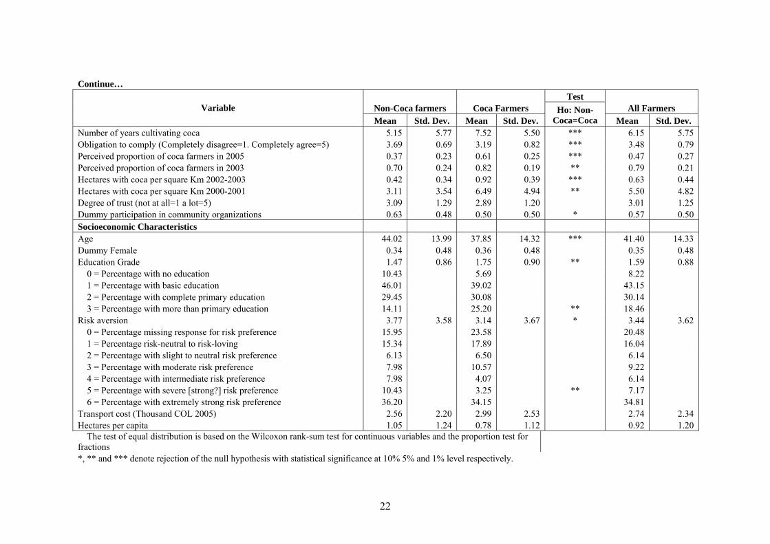
Continue… Test

Non-Coca farmers Coca Farmers All Farmers Variable Mean Std. Dev. Mean Std. Dev.

Ho: Non-Coca=Coca Mean Std. Dev.

Number of years cultivating coca 5.15 5.77 7.52 5.50 *** 6.15 5.75 Obligation to comply (Completely disagree=1. Completely agree=5) 3.69 0.69 3.19 0.82 *** 3.48 0.79 Perceived proportion of coca farmers in 2005 0.37 0.23 0.61 0.25 *** 0.47 0.27 Perceived proportion of coca farmers in 2003 0.70 0.24 0.82 0.19 ** 0.79 0.21 Hectares with coca per square Km 2002-2003 0.42 0.34 0.92 0.39 *** 0.63 0.44 Hectares with coca per square Km 2000-2001 3.11 3.54 6.49 4.94 ** 5.50 4.82 Degree of trust (not at all=1 a lot=5) 3.09 1.29 2.89 1.20 3.01 1.25 Dummy participation in community organizations 0.63 0.48 0.50 0.50 * 0.57 0.50 Socioeconomic Characteristics Age 44.02 13.99 37.85 14.32 *** 41.40 14.33 Dummy Female 0.34 0.48 0.36 0.48 0.35 0.48 Education Grade 1.47 0.86 1.75 0.90 ** 1.59 0.88

0 = Percentage with no education 10.43 5.69 8.22 1 = Percentage with basic education 46.01 39.02 43.15 2 = Percentage with complete primary education 29.45 30.08 30.14 3 = Percentage with more than primary education 14.11 25.20 ** 18.46

Risk aversion 3.77 3.58 3.14 3.67 * 3.44 3.62 0 = Percentage missing response for risk preference 15.95 23.58 20.48 1 = Percentage risk-neutral to risk-loving 15.34 17.89 16.04 2 = Percentage with slight to neutral risk preference 6.13 6.50 6.14 3 = Percentage with moderate risk preference 7.98 10.57 9.22 4 = Percentage with intermediate risk preference 7.98 4.07 6.14 5 = Percentage with severe [strong?] risk preference 10.43 3.25 ** 7.17 6 = Percentage with extremely strong risk preference 36.20 34.15 34.81

Transport cost (Thousand COL 2005) 2.56 2.20 2.99 2.53 2.74 2.34 Hectares per capita 1.05 1.24 0.78 1.12 0.92 1.20

The test of equal distribution is based on the Wilcoxon rank-sum test for continuous variables and the proportion test for fractions *, ** and *** denote rejection of the null hypothesis with statistical significance at 10% 5% and 1% level respectively.

23

coefficient or partial risk aversion. More than half of the sample had high or extremely

high levels of risk aversion.

When the maximum income attainable from cultivating all the available land

with the most profitable legal product is lower than 93,000 pesos per person per month

(the official poverty line) we say that an individual lacks options in the legal economy

in order to survive. Using this definition, 45% of the farmers were classified as lacking

options.

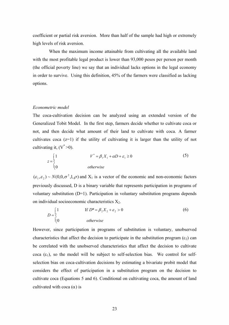
Econometric model

The coca-cultivation decision can be analyzed using an extended version of the

Generalized Tobit Model. In the first step, farmers decide whether to cultivate coca or

not, and then decide what amount of their land to cultivate with coca. A farmer

cultivates coca (z=1) if the utility of cultivating it is larger than the utility of not

cultivating it, (V* >0).

⎪⎩

⎪⎨⎧ ≥++=

=otherwise

DXVz

0

01 111* εαβ

(5)

),1,,0,0(~),( 221 ρσεε N and X1 is a vector of the economic and non-economic factors

previously discussed, D is a binary variable that represents participation in programs of

voluntary substitution (D=1). Participation in voluntary substitution programs depends

on individual socioeconomic characteristics X2.

⎪⎩

⎪⎨⎧ >+=

=otherwise

XDD

0

0* If 1 222 εβ

(6)

However, since participation in programs of substitution is voluntary, unobserved

characteristics that affect the decision to participate in the substitution program (ε2) can

be correlated with the unobserved characteristics that affect the decision to cultivate

coca (ε1), so the model will be subject to self-selection bias. We control for self-

selection bias on coca-cultivation decisions by estimating a bivariate probit model that

considers the effect of participation in a substitution program on the decision to

cultivate coca (Equations 5 and 6). Conditional on cultivating coca, the amount of land

cultivated with coca (α) is

24

⎪⎩

⎪⎨⎧ =+

=otherwise

zX

0

1 If 333 εβα

(7)

We estimate a linear regression model on the amount of land cultivated with coca

conditional on a non-zero investment (Equation 7). Coca farming decisions for 2003

and 2005 were treated as independent of one another, so a pooled data set was used. To

avoid scale effects, monetary related variables such as profits from coca and the best

legal alternative as well as the number of hectares per household, were normalized using

natural logarithms.

Econometric Results

Table 2 presents the predicted signs and estimated coefficients for the seemingly

unrelated bivariate probit model for the coca-cultivation decision, and participation in

agreements of voluntary substitution. The econometric results support the hypothesis of

correlation between unobserved characteristics that affect the decision to cultivate coca,

and that of participating in agreements of voluntary substitution at the 5% significance

level. It is reasonable to think that all farmers face the same market incentives to enter

into coca cultivation and that they are all aware of the high levels of profitability in coca

cultivation compared with legal forms of production. Therefore, if farmers take

different production decisions it must be because they face different opportunities, risks

and needs. Econometric results confirm this hypothesis. Those farmers who had more

opportunities and participated in VAS were less likely to cultivate coca while farmers

that faced higher risks of having coca plants destroyed are significantly less likely to

cultivate coca at 5% significance level and farmers with less land have fewer options to

make a living from legal forms of production which significantly increases their

likelihood of cultivating coca. This suggests that both strategies used by authorities in

Colombia to control coca cultivation, i.e. both eradication and alternative development

programs, have an effect on coca cultivation.

Interestingly, other non-economic factors can explain the decision about

whether to cultivate coca or not, at least to some extent. First, being Protestant, rather

than being Catholic, significantly decreases the likelihood of cultivating coca. One

interpretation is that this might be the result of a change in attitude towards coca

cultivation that has been introduced to the region by the Protestant Churches. This

result suggests that authorities can change people’s attitudes toward coca cultivation by

25

providing them with information about the negative effect that coca has on the

environment, the community, the family and other individuals. Publicity campaigns

and educational programs seem to offer some options. Second, we find that farmers

living in a municipality with more coca are more likely to cultivate. This result points

at the importance on creating social resistance towards coca cultivation and suggest that

authorities should use both local and national campaigns. Third, farmers who have a

higher level of perceived obligation to comply with the law and the authorities are less

likely to cultivate coca. This result indicates that institutional policies can complement

alternative development and eradication programs. For example, the creation of

participative spaces where farmers and authorities negotiate reducing coca cultivation is

an option. Forest Guarding Families (see footnote 7) seem to be a promising option in

this respect. However, the authorities will have to bargain over realistic offers if they are

to ensure that the agreement will be lasting. The process of eliminating the cultivation

of illicit crops has to be gradual in order to allow both farmers and authorities to adjust.

Farmers will need to agree to lower levels of income and probably to returning to

subsistence agriculture because it is simply not possible for the alternatives to compete

in terms of profitability with coca cultivation. The authorities, on the other hand, should

work on creating productive options that allow farmers to make a living. The creation

of price premiums on labels such as “COCA FREE” could be an alternative. The

gradual elimination of illicit crops could also make it possible to generate the social

cohesion needed for the negotiation of community agreements on areas free of coca and

to implement social control mechanisms. The authorities can gain the trust of the

communities by increasing the coverage of the alternative development programs and

the efficiency of their implementation.

Other socioeconomic characteristics of the head of a household such as age,

gender, level of education, degree of risk aversion and distance from the market are not

significant in explaining the decision to cultivate coca. Although not significant, the

likelihood of cultivating coca does decrease with age and level of education, while it

increases for female respondents, distance from the market and level of risk aversion.

Although coca is more risky in terms of having the crops destroyed, legal production

faces lower levels of credit availability, harder market conditions and more price

variability than coca all of which could explain the positive sign on risk aversion.

26

Table 2. Seemingly unrelated bivariate probit

Coca cultivation Decision

Participation in Agreements of Substitution Dependent Variables

n = 329 n = 329

Independent Variables Predicted Signs Coef. Std. Err. Coef. Std. Err.

Log profit coca. - -0.162 0.107 Log profit alternative. ? -0.025 0.084 Index of credit availability and commercialization facility - 0.078 0.075 Sprayed ha/Total ha with coca in municipality - -0.037 ** 0.017 Dummy Atheists -0.178 0.374 -0.005 0.329 Dummy Protestant -0.950 *** 0.326 -0.183 0.306 Years cultivating coca + 0.025 0.017 -0.001 0.017 Moral development. Missing response=0; Pre-Conv=1; Conv=2; Post-Conv=3 - -0.171 0.159 0.124 0.156 Obligation to comply. Completely disagree=1, completely agree=5 - -0.482 *** 0.155 -0.005 0.146 Degree of trust. Not at all=1, a lot=5 - 0.016 0.080 0.193 *** 0.074 Dummy participation in community organizations. - -0.251 0.204 0.393 ** 0.190 Ha with coca/Municipal area. + 0.345 *** 0.063 Cost of transport (Thousand COL) 0.001 0.034 0.019 0.033 Log land per capita ? -0.322 *** 0.095 0.023 0.095 Age -0.021 0.042 0.065 0.040 Squared age 0.000 0.000 0.000 0.000 Female -0.157 0.207 0.268 0.183 Education (None=0,Basic=1, Primary=2, More=3 -0.150 0.414 1.171 *** 0.393 Squared education grade 0.089 0.117 -0.233 ** 0.109 Coefficient of risk aversion (missing response=0,lover=0.84 to extreme=8 0.015 0.028 -0.076 *** 0.025 Dummy missing response level of moral development 1.385 ** 0.614 0.700 * 0.402 Dummy missing response for risk aversion -1.071 1.188 Constant 4.263 *** 1.436 -3.763 *** 1.173 Dummy Orito -1.105 *** 0.251 Dummy Puerto Asis -0.249 0.303 Dummy Valle del Guamuez -1.295 *** 0.351 Rho -0.340 0.123 Likelihood-ratio test of rho=0 chi2(1) 6.750 0.009 *, ** and *** denote statistical significance at 10% 5% and 1% level respectively.

27

On the other hand, participation in agreements of voluntary substitution –VAS-

is explained by the degree of trust in others and participation in community

organizations reflecting the strategy that the program used to reach the beneficiaries.

Similarly, there is a positive effect of age and education on participation in this

program. The negative and significant effect of risk aversion on participation in VAS

may reflect a perception among farmers that the substitution program was risky.

Finally, farmers living in Orito and Valle are significantly less likely to participate in

VAS compared with farmers from Mocoa, which indicates that substitution programs

were directed to areas with better accessibility.

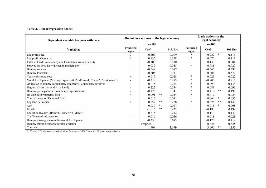
Our theoretical model predicts that the effect of economic and non-economic

factors will differ according to whether farmers lack options in the legal economy or

not. To test the predictions of the model, we run independent regressions for farmers in

both groups. Table 3 presents the predicted signs from the theoretical model and the

estimated coefficients of a linear regression model on hectares cultivated with coca for

both groups. We find that irrespective of whether farmers lack options in the legal

economy or not, those who have larger farms cultivated more hectares with coca. This

could indicate that the high cost of production restricts smaller farmers from engaging

in coca cultivation. We find some evidence for the effect of social norms on the

decision to cultivate. Farmers who do not lack alternatives in the legal economy

cultivate a larger amount of coca if they live in a municipality with higher levels of coca

cultivation. For farmers who lack options in the legal economy, we find that

participation in community organizations increases the amount of land that is cultivated

with coca. These two effects may indicate a degree of social acceptance of coca

cultivation in the area. It is also interesting to note that in the case of farmers who lack

alternatives in the legal economy, the perception that there is a higher profit to be made

from coca reduces the amount of coca that is cultivated. This could indicate that the

coca-cultivation decisions depend on subsistence needs. As coca is more profitable,

they can survive with only a few hectares given over to coca cultivation. More evidence

for the positive correlation between lack of options and coca cultivation is provided by

the positive correlation between the cost of traveling to market and coca cultivation.

Other socioeconomic characteristics that are significant in explaining the amount of

land cultivated with coca are age and the dummy for female respondents.

28

Table 3. Linear regression Model

Do not lack options in the legal economy Lack options in the legal economy Dependent variable hectares with coca

n=106 n=108

Variables Predicted signs Coef. Std. Err. Predicted

signs Coef. Std. Err.

Log profit coca ? -0.107 0.209 ? -0.222 * 0.116 Log profit Alternative ? 0.135 0.198 ? 0.070 0.111 Index of Credit Availability and Commercialization Facility -0.100 0.130 0.133 0.084 Sprayed ha/Total ha with coca in municipality - 0.032 0.045 + -0.031 0.027 Dummy Atheists -0.549 0.697 -0.565 0.390 Dummy Protestant -0.505 0.911 0.004 0.572 Years cultivating coca + 0.019 0.028 ? 0.025 0.022 Moral development (Missing response=0; Pre-Conv=1; Conv=2; Post-Conv=3) - -0.218 0.295 ? -0.205 0.215 Obligation to comply (Completely disagree=1, Completely agree=5) - -0.015 0.234 ? 0.093 0.136 Degree of trust (not at all=1, a lot=5) - 0.222 0.134 ? 0.089 0.096 Dummy participation in community organizations - -0.173 0.341 ? 0.417 ** 0.199 Ha with coca/Municipal area + 0.091 ** 0.044 ? 0.017 0.024 Cost of transport (Thousand COL) 0.015 0.091 0.064 * 0.035 Log land per capita + 0.557 ** 0.228 ? 0.326 ** 0.149 Age -0.030 * 0.017 -0.015 * 0.008 Female -1.015 ** 0.422 -0.183 0.199 Education (None=0,Basic=1, Primary=2, More=3 0.215 0.212 -0.113 0.140 Coefficient of risk aversion - 0.010 0.046 0.018 0.028 Dummy missing response for moral development -0.330 0.695 -0.170 0.419 Dummy missing response for risk aversion dropped 0.446 0.825 Constant 1.909 2.699 3.000 ** 1.153 *, ** and *** denote statistical significance at 10% 5% and 1% level respectively.

21

From a policy perspective, our results suggest that eradication and alternative

development are effective in reducing the incentive to start cultivating coca but have a

smaller role in affecting the amount of coca that is cultivated.

5. Conclusions

In this paper we explain the decision to cultivate coca and the amount of land that is

cultivated both from a theoretical and empirical perspective. We develop a behavioral

version of the economic model of crime to explain coca farming decisions.

Our model also considers situations in which farmers cannot make a living

from legal activity. Coca is cultivated because it is more profitable than the legal

alternatives, but also because this relative profit is tempting enough to compensate for

the personal and social disapproval that coca cultivation generates. Therefore, higher

moral standards or higher levels of social pressure reduce the likelihood of cultivating

coca. This suggests that in addition to policies of eradication and alternative

development, authorities can increase the population’s awareness of the negative effects

of coca cultivation in order to discourage the activity. Authorities can gain better

support if policies are regarded as necessary and if the public recognize the efficiency,

fairness and transparency in the policies. Increasing coverage of the existing programs

and negotiating gradual reductions in areas can be some of the mechanism that

authorities can use to gain public’s trust. We find evidence that marginality and the

impossibility of making a living out of legal activities is a strong factor behind coca

cultivation. In this case, the emphasis of the policy should be towards increasing the

profitability of legal agriculture by, for example, investing in infrastructure or offering

minimum prices for legal products. Our model suggests that farmers reduce coca

cultivation in response to both eradication and VAS.

Using self-reported information on an illicit activity such as coca cultivation

may underestimate the dimensions of the problem of coca cultivation. However, our

intention has been to unveil some of the factors that affect coca cultivation that cannot

be studied with aggregated information. We consider that this study is a first step

towards understanding the effect of motivational factors on coca cultivation and is

meant to be indicative for alternative strategies that could be used by the authorities.

22

6. References Aguirre, Eduardo. 2003. “Juicio moral presente en delincuentes menores: Estudio para la Alcadía mayor

de Bogota.” Universidad Nacional de Colombia. Akerlof, George A. 1997. “Social distance and Social Decisions.” Econometrica. 65 (September): 1005-

28. Akpalu, Wisdom. 2006. “Individual discount rate and regulatory compliance in a developing country

fishery.” Doctoral thesis. School of business, economics and law. Göteborg University. Alvarado, Luis E. Yilberto Lahuerta. 2005. “Comportamiento del Gasto del Estado Colombiano en la

Lucha contra las Drogas: 1995 – 2004.” Dirección Nacional de Estupefacientes – DNE, Departamento Nacional de Planeación, DNP. Bogota, Colombia.

Becker, Gary. 1968. “Crime and Punishment: An Economic Approach.” Journal of Political Economy. 76 (March-April): 169-217.

Binswanger, Hans. 1980. “Attitude towards risk: Experimental Measurement in Rural Area.” American Journal of Agricultural Economics. 62 (August): 395-407.

Calvó-Armengol, Antoni and Yves Zenou. 2004. “Social Networks and Crime Decisions: The Role of Social Structure in facilitating delinquent behavior.” International Economic Review. 45 (August): 939-58.

Carvajal, Maria Paula. 2002. “Factores explicativos de la presencia de cultivos ilícitos en los municipio de Colombia” Dissertation paper to opt to the title in the master in environmental economics. CEDE- Universidad de los Andes. Bogotá, Colombia.

Dawes, Robin and David Messick. 2000. “Social dilemmas.” International Journal of Psychology, 35 (April): 111-16.

Díaz, Ana Maria and Fabio Sánchez. 2004. “Geography of Illicit Crops and Armed conflict in Colombia” Document CEDE 2004-18 Issn 1657-7191. (March)

DNE. 2005. “Acciones y Resultados 2005” Dirección Nacional de Estupefacientes – DNE, Bogota, Colombia.

Easton, David. 1958. “The perception of authority and political change.” In Carl J. Friedrich ed. Authority. Cambridge: Harvard University Press.

Ehrlich, Issac. 1973. “Participation in illegitimate activities: a theoretical and empirical investigation.” Journal of political economy. 81 (May-June): 521-565.

Eide, Erling in cooperation with Jørgen Assness and Terje Skjerpen. 1994. “Economics of crime: Deterrence and the rational offender.” Contributions to economic analysis 227. North Holland.

Eisenhauer, Joseph G. 2004. “Economic Models of Sin and Remorse: Some Simple Analytics.” Review of Social Economy, 62(June): 201-19.

Elster, Jon. 1989. ‘‘Social Norms and Economic Theory’’ Journal of Economic Perspectivas, 3 (Autumn): 99-118.

Frey, Bruno. 1997. “Not just for the money: and economic theory of personal motivation.” Edward Elgar Publishing. Cheltenham UK.

García, Guillermo. 2000. “Estrategia de Desarrollo alternativo en Colombia.” En Cultivos Ilícitos en Colombia. Memorias del foro realizado el 17 y 18 de Agosto de 2000. Universidad de los Andes. Bogotá, Colombia.

Garoupa, Nuno. 1997. “The Role of Moral values in the economic analysis of crime: a General equilibrium approach.” Universitat Pompeu Fabra and Standfort Law School. Working papers series 245.

Garoupa, Nuno. 2003. “Crime and Social Norms.” Portuguese Economic Journal. 2 (December): 131-144.

Glaeser, Edward L. Bruce Sacerdote and Jose Scheinkman. 1996. “Crime and Social Interactions.” Quarterly Journal of Economics. 111 (May): 508–48.

Harrison Glenn W. and John List. 2004. “Field experiments.” Journal of Economic Literature, 42 (December): 1009 1055.

Hatcher, Aaron, Shabbar Jaffry, Olivier Thébaud, and Elizabeth Bennett. 2000. “Normative and Social Influences Affecting Compliance with Fishery Regulations.” Land Economics. 76 (August): 448-61.

Hausman, Daniel and Michael McPherson. 1993. ‘‘Taking Ethics Seriously: Economics and Contemporary Moral Philosophy.’’ Journal of Economic Literature, 31 (June): 671-731.

Huang, Chien Chieh, Derek Laing and Ping Wang. 2004. “Crime and Poverty A search theoretical approach” International Economic Review. 45 (August): 909-38.

23

Kohlberg, Laurence. 1969. “Stage and sequence: The cognitive developmental approach to socialization.” In: D. Goslin, ed., Handbook of socialization theory and research. Chicago: Rand McNally, pp. 347-480.

Lind, George, Hans A. Hartmann and Roland Wakenhut (Eds). 1985. “Moral Development and the Social Environment Studies in the Philosophy and Psychology of Moral Judgment and Education”.

Mocan, Naci, Stephen Billups and Jody Overland. 2005. “A Dynamic Model of Differential Human Capital and Criminal Activity.” Economica. 72 (November): 655-81.

Moreno Sánchez, Rocio, David S. Kraybill and Stanley R. Thompson. 2003. “An econometric analysis of coca eradication policy in Colombia.” World Development. 31 (February): 375-383.

Moya, Andrés. 2005. “Impacto de la erradicación forzosa y el desarrollo alternativo sobre los cultivos de coca.” Dissertation paper to opt to the title in the master program in economics. Economics Department. Universidad de los Andes. Bogotá, Colombia.

Murphy, Kevin, Andrei Schleifer and Robin Vishny. 1993. “Why is rent seeking so costly to growth.” American Economic Review, 83 (May): 409-414.

ONDCP. 2006. “The Economic cost of drug abuse in the USA 1992-2002.” Office of National Drug Control Policy. Washington. United States of America.

Opp, Karl D. 1979. “The emergence and effects of Social Norms. A confrontation of some hypothesis of sociology and economics.” Kyklo., 32 (4): 775-801.

Ortíz, Cesar. 2000. “La Estrategia del Programa de Desarrollo Alternativo en Colombia” En Cultivos Ilícitos en Colombia. Memorias del foro realizado el 17 y 18 de Agosto de 2000. Universidad de los Andes. Bogotá, Colombia.

Rocha, Ricardo and Maria Clemencia Ramírez. 2006. “Impactos de la economía ilícita de la droga: el caso de Colombia.” Study prepared to USAID.

Sah, Raaj. 1991. “Social Osmosis and Patterns of Crime.” Journal of Political Economy. 99 (December): 1272–95.

Schrag, Joel and Susana Scotchmer. 1997. “The Self reinforcement nature of crime.” International review of law and Economic. 17(September): 325-335.

Starmer, Chris. 2000. “Developments on non-expected utility theory: the Hunt of a descriptive theory of choice under risk.” Journal of Economic Literature. 38 (June): 332-382.

Sutinen, Jon and K. Kuperan. 1999. “A Socio-Economic Theory of Regulatory Compliance.” International Journal of Social Economics. 26 (1/2/3): 174-193.

Tabares, Elizabeth and Ramón Rosales. 2004. “Políticas de control de oferta de coca: La zanahoria y el garrote.” Document CEDE 2005-10. Universidad de los Andes. Bogotá, Colombia.

Thoumi, Francisco. 2000. “Illegal drugs in Colombia: from illegal economic boom to social crisis.” The Annals of the American Academy of Political and Social Science. 582 (January): 102-16 .

Tversky, Amos and Daniel Kahneman. 1992. “Advances in Prospect Theory: Cumulative Representation of Uncertainty”. Journal Risk and Uncertainty, 5 (October): 297-323.

Tyler, Tom R. 1990. “Why People Obey the Law”. New Haven, CT: Yale Univ. Press. Tyran, Jean-Robert and Lars P. Feld. 2002. “Why people obey the law experimental evidence from the

provision of public goods.” CESifo Working Paper No. 651. University of St Gallen (January) Uribe, Sergio. 2005. “Documento metodológico de los productos hoja de coca y base de coca” Study

prepared to Dirección Nacional de Estadística – DANE. Bogotá, Colombia. Williams, Jenny and Robin C. Sickles. 2002. “An analysis of crime as a work model evidence from the

1958 Philadelphia birth cohort study." Journal of Human Resources 37(Summer): 479-509.

24

Appendix A. Model

Coca is cultivated if: 0))(()()()1(Y >∏+−+−= LWUYpUYUp lbg . This implies

the following partial effects on the decision of whether to cultivate coca or not.

0))1())(´()´()1(( i <∏−−+−=∂∂ γ

λ bg YpUYUpY

(1.1)

0))1())(´()´()1(( i <∏−−+−=∂∂ λ

γ bg YpUYUpY

(1.2)

0))())(´()´()1(( 2 <−−+−=∂∂ αatYpUYUp

qY

bg

(1.3)

0))())(´()´()1(( 2 <−−+−=∂∂ αaqYpUYUp

tY

bg

(1.4)

0 )()( <+−=∂∂

bg YUYUpY (1.5)

0F if 0)´( f ><−=∂∂

fb FYpUfY (1.6)

?))´()´()´()1(( =∏−+−=∂∂

llLbgl

YUYpUYUpYππ

(1.7)

0))´()´()1(( >∏+−=∂∂

iibgi

YpUYUpYππ

(1.8)

?)´()´()´()1( =−+−=∂∂

Lbg YUYpUYUpWY (1.9)

?)))(´()´()´()1(( =−+−=∂∂

lLlbg YUYpUYUpLY π

(1.10)

When both coca and the legal product are cultivated, the first order condition for an

interior solution implies:

0

))1(')(2)1)(1)((('

))1(')(2)1)(1)(((')1(V

i

i

=+=

−∏−−−−−−−

+∏−−−−−−−−=∂∂

BA

faqtYpU

aqtYUp

lib

ligi

γλαππγλ

γλαππγλα

(3.1)

Where:

li,kfor 0 =>=∂∏∂

kk π

α

0 >=∂∂ fFα

b g,zfor )(')(==

∂∂

zz YUYU

α

25

0))1(')(2)1)(1)((('

0))1(')(2)1)(1)(((')1(

i

i

<−∏−−−−−−−=

>∏−−−−−−−−=

faqtYpUB

aqtYUpA

lib

lig

γλαππγλ

γλαππγλ

The second order condition for maximization implies:

0 ')(' ')(')1()(" )(")1( 222

2

<Δ=+−++−=∂∂ bYpUaYUpbYpUaYUpV

bgbgα (3.2)

Where,

0))1(')(2)1)(1((

0))1(')(2)1)(1((

i

i

<−∏−−−−−−−=

>∏−−−−−−−=

faqtb

aqta

li

li

γλαππγλ

γλαππγλ

;';' bddba

dda

==αα

Deriving equation (3) with respect to α and λ and solving we obtain:

[ ]

[ ] ))1(')1))(((')(')1(( ))()(()1(1

))1(')1))(((')(')1(( )1)()(")(")1((1

iibgbgi

iibgibg

YpUYUpBYRYR

YpUYUpbYpUaYUp

∏−+−+−+−∏−Δ

=

∏−+−+−+∏−+−Δ

=∂∂

γλπγγ

γλπγγλα

λ

λ

where, R(Yz) is the coefficient of absolute risk aversion, )(')(YU")(

z

zz YU

YR −= . We assume that if

subsistence is covered, U”<0 farmers have decreasing absolute risk aversion – DARA-, R(Yb) > R(Yg) >

0. If subsistence is under threat, we consider that U”>0 and assume decreasing absolute risk preferences

– DARP- , R(Yb) < R(Yg).<.0.

⎩⎨⎧

><<

∂∂

DARP 0; U"if ? DARA 0; U"if 0

is λα

(4.1)

Similarly, it is possible to show that

[ ] )')1))(((')(')1(( )1())()((1iibgibg YpUYUpBYRYR ∏−−+−+∏−−

Δ=

∂∂ λπλλ

γα

⎩⎨⎧

><

∂∂

DARP 0; U"if ?DARA 0; U"if ?

is γα

(4.2)

26

[ ])(2))(')(')1(())(())()((1 2 atYpUYUptBYRYRq bgbg −+−+−−

Δ=

∂∂ αααα

DARP 0; U"if0DARP 0; U"if?DARA 0; U"if?DARA 0; U"if0

is

⎪⎪⎩

⎪⎪⎨

⎧

<>><><<<<<

∂∂

aa

aa

qα

αα

αα

(4.3)

[ ])(2))(')(')1(())(())()((1 2 aqYpUYUpqBYRYRt bgbg −+−+−−

Δ=

∂∂ αααα

⎪⎪⎩

⎪⎪⎨

⎧

<>><><<<<<

∂∂

aa

aa

tα

αα

αα

DARP 0; U"if0DARP 0; U"if?DARA 0; U"if?DARA 0; U"if0

(4.4)

[ ] 0 )(' )('1<+−

Δ−

=∂∂ bYUaYU

p bgα

(4.5)

[ ]⎩⎨⎧

><<

+Δ

=∂∂

⋅ 0 U"if ?0 U"if 0

is )(')bF(Y"1 fb bYpUpUfα for Ff > 0 (4.6)

⎩⎨⎧

><<

∂∂

DARP ;0 U"if 0DARA 0; U"if ?

is lπ

α 0 if >∏ lπ

(4.7)

[ ]ii ibgibg

i

YpUYUpBYRYR ππ γλγλγλπα

∏−−−−+−+∏−−−Δ−

=∂∂ )1(')1)(1))(((')(')1(( )1)(1())()((1

⎩⎨⎧

><

∂∂

DARP 0; U"if ? DARA 0; U"if ?

is iπ

α 0 if >∏iiπ

(4.8)

][⎩⎨⎧

><<>

−Δ−

=∂∂

DARP 0; U"if 0DARA 0; U"if 0

is ))()((1 BYRYRW bgα (4.9)

][ )))(´()´()1(( ))( )((1,LlbglLbg YpUYUpBYRYR

Lπα

+−−∏−Δ−

=∂∂

[ ])(')(')1( ))()((1 bglbgl

YpUYUpBYRYR +−+∏−−Δ

=∂∂

ππα

27

0;0when DARP 0; U"if ?

DARA 0; U"if 0 is , <>∏⎩⎨⎧

<<>

∂∂

LllLLπα

(4.10)

Appendix B. Survey

28

29

30

31

32

33

A choice experiment on coca cropping12 Marcela Ibanez13

Department of Economics Göteborg University

Abstract

Between 1997 and 2005, 5.2 billion USD were invested to reduce cocaine

production in Colombia, the world’s main cocaine producer. However, since little is

known about the effectiveness of policies targeting coca cultivation, this paper evaluates

the efficiency of the two main ones: eradication and alternative development. We

measure the responsiveness of farmers to eradication and alternative development

programs using a survey based experiment. Our results support Becker’s (1968) model

of crime participation and in addition shed light on other non-economic factors that

affect the coca cultivation decision. Social norms, legitimacy, and poverty are found to

be affecting coca cultivation. The analysis concludes that it is more cost-efficient to

spend money on increasing the risk of eradication than on alternative development,

although any potential negative external effects of eradication are ignored.

Keywords: Illegal drugs, Choice experiment, Colombia. JEL classification: G11, K42, Z12, Z13

12 Acknowledgements: Financial support from the Swedish Agency for International Development Cooperation (Sida) to the Environmental Economics Unit at Göteborg University is gratefully acknowledged. The paper has benefited from comments and discussions with Fredrik Carlsson, Håkan Eggert, Katharina Nordblom, Francisco Alpizar, and seminar participants at Göteborg University 13 Department of Economics, Göteborg University, Box 640, SE-40530 Göteborg, Sweden. Tel: + 46 31 773 46 69, e-mail: marcela.ibanez@economics.gu.se

34

1. Introduction

Cocaine is the most commonly consumed illegal drug in the world after marijuana.

Around 13 million people use it, and contrary to what many believe, cocaine

consumption is a problem in both developed and developing countries (UNDCP, 2005).

Cocaine production, on the other hand, is highly concentrated; more than 98% of the

total cultivated area is located in Colombia, Peru, and Bolivia. In the 1980s, following

three international conventions on narcotic drugs (UN, 1961, 1971, 1988) a campaign

against transformation and trafficking of drugs was initiated in Colombia. Despite the

successful dismantling of the two main Colombian drug cartels the Colombia cocaine

production started a dramatic growth, from less than 10% of the total production areas

in the early 1990’s production increased to 74% in 2000. As a response, policies of

eradication and alternative development were implemented to control coca cultivation.

Eradication, or destruction, of coca plants by aerial spraying of herbicides or by pulling

the plants manually aims at increasing the risk of cultivating coca. Alternative

development, on the other hand, aims at increasing the profitability of legal crops by

investing in infrastructure and providing subsidized credits and technological support.

An astonishing 5.2 billion USD was spent on the war on drugs in Colombia between

1997 and 2005, but the production of cocaine nevertheless increased from 350 to 640

tons during the same period (ONDCP, 2006; UNDCP, 2006). Although the cost of anti-

drug policies constitutes 1% of the Colombian GDP, surprisingly little is known about

the effectiveness of the Colombian anti-drug policies. This paper contributes to the

limited literature that evaluates the effectiveness of eradication and alternative

development to control coca cultivation. To study economic and non-economic factors

behind participation in the illegal coca production, we use unique household level data

on Colombian farmers.

Previous empirical studies have tried to evaluate the effectiveness of eradication

and alternative development (e.g., Carvajal, 2000; Moreno et al., 2002; Tabares and

Rosales, 2005), but face many problems. First, aggregated information does not allow

identification of behavioral factors affecting the decision to get involved in illegal

activity. Second, policy levels based on historical and regional information are

endogenous, and third, the use of matching estimators does not allow evaluating the

35

effects of different policy levels (e.g., Díaz and Sánchez, 2004; Moya, 2005). More

generally, the use of revealed data limits the analysis to the effects of the policy levels

that have actually been implemented, while it is hard to predict the effects of

significantly different policy levels.14 An alternative approach to deal with the above

problems is to use survey-based experiments where coca farmers indicate how they

would behave under various anti-drug policies. This type of stated preference method

has commonly been applied to areas such as environmental economics, health

economics, and tax compliance; see for example Alpizar et al. (2003), Louviere et al.

(2000), and Trivedi et al. (2005).

The objective of this paper is to study the effect of economic and non-economic

factors on coca cultivation. We use a hypothetical choice experiment on coca

cultivation where respondents state how many hectares they would dedicate to coca at

different levels of the relative profitability of the best alternative and of the probabilities

of having the plants eradicated. Since the policy levels are varied, we can identify the

separate effects of each policy after controlling for other factors affecting coca

cultivation. In particular, following the behavioral model of crime we consider the

effect of (1) social norms (e.g., Glaeser et al., 1996; Calvó-Armengol and Zenou, 2004;

Garoupa, 2003 ; Frey, 1997; Elster, 1998), (2) morality (e.g.,; Hausman and McPherson,

1993; Sutignen and Kuperan, 1999; Eiseihauer, 2004), and (3) legitimacy (e.g., Tyler,

1990; Feld and Tyran, 2002; Feld and Frey, 2005). Our sample consists of both coca

and non-coca farmers living in Putumayo, one of the regions with a long tradition of

coca cultivation in Colombia. Obviously, there are a number of problems in applying a

survey-based questionnaire to something as sensitive as coca farming. Nonetheless, we

believe that the approach can serve as a good complement to studies using actual

behavior.

The rest of the paper is organized as follows. Section 2 presents the model,

Section 3 the survey design, and Section 4 the econometric model. Section 5 reports the

results, and Section 6 concludes the paper.

14 Others (e.g., Kennedy et al., 1993; Riley, 1991) have used an economic model of cocaine production and consumption to simulate the effects of increases in eradication and alternative development, but the measure of effectiveness has then been assumed rather than measured.

36

2. A Simple Model of Coca Cropping

The decision to cultivate coca can be analyzed in the framework of traditional models of

crime (e.g., Becker, 1968; Ehrlich, 1973; Allingham and Sandmo, 1972). Farmers

decide how to allocate their land and labor between coca and an alternative crop.

Though coca is more profitable than the alternative, it is also more risky. Coca

cultivation is illegal, and authorities may discover and destroy the plants with a

probability p. If coca plants are discovered and destroyed, farmers lose their

investments and the land is incapacitated, preventing production in the next period. This

loss is represented by the cost F.15 Following the traditional models of crime, farmers

will cultivate coca if the expected marginal profit from coca cultivation, ΠCoca, net of

the opportunity cost of cultivating coca, ΠAlternative, is greater than the expected marginal

cost of having the plants destroyed, pF. In addition, the models imply that the amount

of land cultivated with coca depends not only on expected costs and benefits but also on

a farmer’s risk preferences.

Empirical evidence largely supports the predictions of the traditional models of

crime (Cameron, 1988; Freeman, 1999; Eide et al., 2006). However, these models fail

to explain why people self-report taxable income correctly, pay TV licenses, or abstain

from breaking the law even though the expected cost of being detected is very low (e.g.,

Frey and Torgler, 2004; Cohen, 1999; Andreoni et al., 1998). To explain the departure

from self-interested behavior in the rational choice models, the behavioral models of

crime consider other non-economic factors affecting participation in illegal activity. For

example, Elster (1989), Posner (1997) and Bowles and Gintis. (1998) propose that in

addition to economic incentives, social norms promote social order. Reputation, stigma,

shame, and eventually ostracism serve to sustain the social norms and combat antisocial

behavior. On the other hand, Frey (1997), Torgler (2002), and Sutinen and Kuperan

(1999), among others, suggest that morality or the intrinsic motivation to do the “right

thing” explains why people comply with regulations. A third type of explanation of

high compliance levels suggests that compliance with the law depends not only on the

internal sense of right or wrong, but also on legitimacy or acceptance of the law and

support of the authorities (e.g., Tyler, 1990; Feld and Frey, 2005; Feld and Tyran,

1990). People’s compliance increases when they perceive the authorities and the law to

15 In Colombia, the law also dictates imprisonment although this policy is seldom used.

37

be fair, and when they participate in deciding the law. In summary, the supply function

of coca, C, is

C = f(ΠCoca , ΠAlternative, p, F, S, M, L),

where S refers to social norms, M to morality, and L to legitimacy or acceptance of the

authorities.

3. The Survey

We used a survey based experiment to measure the responsiveness of farmers to

changes in relative profit of an alternative crop and changes in the probability of

eradication. The survey included a number of questions regarding land holdings,

profitability of coca and the best alternative, and perceptions of coca cultivation. In

addition, to capture the effect of non-economic factors and individual socioeconomic

characteristics, the survey included the Moral Judgment Test (Lind et al., 1985),

attitudinal questions on coca production and anti-drug policies, and a risk experiment.

We carefully informed the participants of the academic nature of the study, ensured

anonymity, and that all data from the study was confidential and would be revealed only

to the research team.

The choice experiment

In the choice experiment, we asked the respondents to state how many hectares they

would dedicate to coca at various levels of two attributes: the relative profitability of the

best alternative crop and the risk of eradication. This open-ended question allowed for

zero coca cultivation or cultivation of more hectares than actual land holdings,

reflecting the fact that the land market is competitive. When the profit from coca

cultivation is good, farmers rent or buy land to establish coca crops. Attribute levels

were customized based on the current situation of the farmer in order to make the choice

situation more realistic and familiar for the respondents. The respondents were first

reminded of their answers to the questions about how much coca they crop today, the

profitability of coca and the best alternative, and their perceived risk of having coca

crops destroyed. Figure 1 outlines the scenario.

38

Figure 1. Scenario of the choice experiment.

In the next section, I would like to ask what you would do if the profitability of

the best alternative to coca were different and if the risk of having the crops

destroyed changed. I would like you to think what you would have done if the

situation were different. In this type of study, people tend to answer in the way

they think the researcher wants rather than what they would really do. Please

consider carefully what you would do if you had to make these decisions. There

are no wrong or right answers; it is all a matter of your own preferences. Take

into consideration that others would probably do the same as you.

You said that last year you had …… ha with coca and that the profit from 1 ha

coca was …… while the profit from the best alternative was …… In addition,

you said that the risk of having your crops completely destroyed by authorities

was …… Assuming that everything else is the same as last year, how many

hectares would you plant with coca if the profit from 1 ha of coca were the

same as today, but the profit of the best alternative were …… and the risk of

having the crops destroyed were ……

Each participant answered at most the nine choice sets described in Table 1. They

combined three levels of profitability for the alternatives: same as today, higher than

today, and lower than today; and three levels of risk of eradication: higher than today,

lower than today, and zero. The levels were presented in absolute terms as described

below.

Table 1. Description of choice sets. Choice set Profitability of best

alternative Risk of having crops destroyed

1 Same as today Higher risk than today 2 Lower than today Higher risk than today 3 Higher than today Higher risk than today 4 Higher than today Lower risk than today 5 Same as today Lower risk than today 6 Lower than today Lower risk than today 7 Lower than today Zero risk 8 Higher than today Zero risk 9 Same as today Zero risk

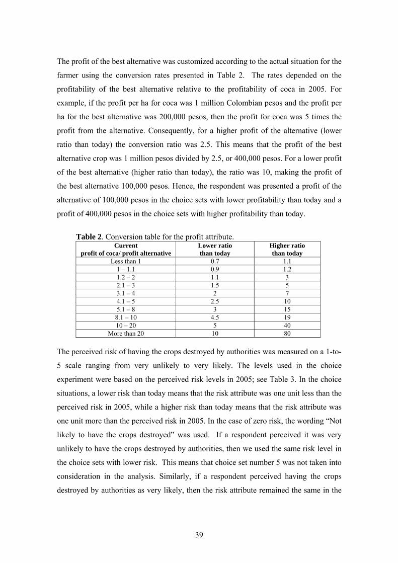
39

The profit of the best alternative was customized according to the actual situation for the

farmer using the conversion rates presented in Table 2. The rates depended on the

profitability of the best alternative relative to the profitability of coca in 2005. For

example, if the profit per ha for coca was 1 million Colombian pesos and the profit per

ha for the best alternative was 200,000 pesos, then the profit for coca was 5 times the

profit from the alternative. Consequently, for a higher profit of the alternative (lower

ratio than today) the conversion ratio was 2.5. This means that the profit of the best

alternative crop was 1 million pesos divided by 2.5, or 400,000 pesos. For a lower profit

of the best alternative (higher ratio than today), the ratio was 10, making the profit of

the best alternative 100,000 pesos. Hence, the respondent was presented a profit of the

alternative of 100,000 pesos in the choice sets with lower profitability than today and a

profit of 400,000 pesos in the choice sets with higher profitability than today.

Table 2. Conversion table for the profit attribute.

Current profit of coca/ profit alternative

Lower ratio than today

Higher ratio than today

Less than 1 0.7 1.1 1 – 1.1 0.9 1.2 1.2 – 2 1.1 3 2.1 – 3 1.5 5 3.1 – 4 2 7 4.1 – 5 2.5 10 5.1 – 8 3 15

8.1 – 10 4.5 19 10 – 20 5 40

More than 20 10 80 The perceived risk of having the crops destroyed by authorities was measured on a 1-to-

5 scale ranging from very unlikely to very likely. The levels used in the choice

experiment were based on the perceived risk levels in 2005; see Table 3. In the choice

situations, a lower risk than today means that the risk attribute was one unit less than the

perceived risk in 2005, while a higher risk than today means that the risk attribute was

one unit more than the perceived risk in 2005. In the case of zero risk, the wording “Not

likely to have the crops destroyed” was used. If a respondent perceived it was very

unlikely to have the crops destroyed by authorities, then we used the same risk level in

the choice sets with lower risk. This means that choice set number 5 was not taken into

consideration in the analysis. Similarly, if a respondent perceived having the crops

destroyed by authorities as very likely, then the risk attribute remained the same in the

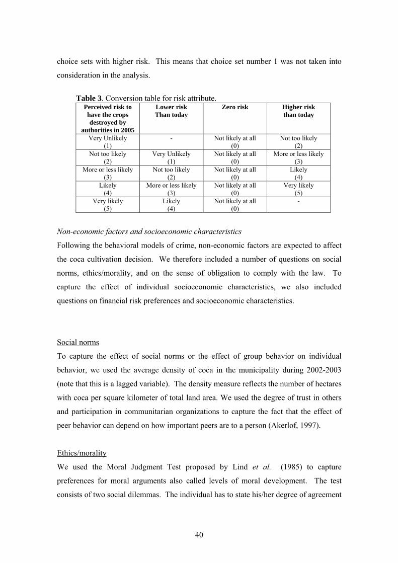
40

choice sets with higher risk. This means that choice set number 1 was not taken into

consideration in the analysis.

Table 3. Conversion table for risk attribute.

Perceived risk to have the crops destroyed by

authorities in 2005

Lower risk Than today

Zero risk Higher risk than today

Very Unlikely (1)

- Not likely at all (0)

Not too likely (2)

Not too likely (2)

Very Unlikely (1)

Not likely at all (0)

More or less likely (3)

More or less likely (3)

Not too likely (2)

Not likely at all (0)

Likely (4)

Likely (4)

More or less likely (3)

Not likely at all (0)

Very likely (5)

Very likely (5)

Likely (4)

Not likely at all (0)

-

Non-economic factors and socioeconomic characteristics

Following the behavioral models of crime, non-economic factors are expected to affect

the coca cultivation decision. We therefore included a number of questions on social

norms, ethics/morality, and on the sense of obligation to comply with the law. To

capture the effect of individual socioeconomic characteristics, we also included

questions on financial risk preferences and socioeconomic characteristics.

Social norms

To capture the effect of social norms or the effect of group behavior on individual

behavior, we used the average density of coca in the municipality during 2002-2003

(note that this is a lagged variable). The density measure reflects the number of hectares

with coca per square kilometer of total land area. We used the degree of trust in others

and participation in communitarian organizations to capture the fact that the effect of

peer behavior can depend on how important peers are to a person (Akerlof, 1997).

Ethics/morality

We used the Moral Judgment Test proposed by Lind et al. (1985) to capture

preferences for moral arguments also called levels of moral development. The test

consists of two social dilemmas. The individual has to state his/her degree of agreement

41

with a series of arguments that justify or oppose the actions taken in the dilemma.

According to the level of reasoning used to justify moral dilemmas and following the

theory of moral development, individuals can be classified into three levels of moral

development (Kohlberg, 1969). At the lowest level of moral development, pre-

conventionalists base their arguments on individualistic reasons (rewards and

punishment). At the second level, conventionalists base their moral arguments on social

reasons (social norms or maintaining social order), and in the last level of moral

development, post-conventionalists motivate their arguments in terms of higher reasons

(human rights and justice). In addition to level of moral development, we use religiosity

to capture morality. Colombia is a mainly Catholic country, but in recent years there has

been a rapid expansion of Protestantism, which has renewed religious enthusiasm.

Given the dynamics of these new churches, we want to investigate how they have

affected coca cultivation.

Sense of obligation to comply with the law

To capture the effect of legitimacy (acceptance of the authorities and the law) on the

decision to cultivate coca, we used a measure of conformity with the law. This measure

captures the degree of acceptance of a series of statements relative to the existence of

the law, fairness of the authorities, participation in defining rules, and effectiveness of

rules.

Financial risk preferences

To capture financial risk preferences likely to affect the decision to cultivate coca and

the amount of coca that is cultivated, we used a simple risk experiment that follows

Binswanger’s (1980) design. Table 4 presents the design used in the risk experiment.

Participants in the survey were asked to state whether they prefer to crop Option A or

Option B, which are equivalent in terms of investment and required effort, but differ in

profits. The second column in Table 4 describes Option A, which always gives a profit

of 1 million pesos (equivalent to 400 USD), whereas Option B yields equal chances

between a higher or a lower profit. Each participant answered the five choice sets

presented in Table 4. The first choice set where a participant switched from Option B to

42

Option A allows us to calculate a coefficient of risk aversion if we assume the following

functional form of the utility function:

ρ

ρ

−=

−

1)(

1XXU ,

where ρ represents the coefficient of relative risk aversion and X the certainty

equivalent of the prospect.

Table 4. Choice sets in risk experiments, profit in thousand Colombian pesos.

Choice set Option A Option B Maximum and Minimum Rho if A is preferred to B in this

and subsequent choices Lower

Prob=0.5 Higher

Prob=0.5

1 1 000 000 900 000 1 800 000 7.500 – 3.615 2 1 000 000 800 000 2 400 000 3.615 – 1.189 3 1 000 000 600 000 3 000 000 1.189 – 0.506 4 1 000 000 200 000 3 800 000 0.506 – 0.168 5 1 000 000 0 4 000 000 0.168 – 0.000

4. Econometric Model

The decision to cultivate coca can be seen as a two-step procedure where farmers first

decide whether to cultivate coca or not, and then given that coca is cultivated decide on

the number of hectares to cultivate. We will treat these two decisions as separate

decisions.16 The expected indirect utility of coca cultivation for individual i in choice

situation t is given by:

itiCocai

eAlternativit

tit zPDetectionV εβαα ++Π

Π+= '21 .

The first two variables are the attributes that we are interested in evaluating in the

choice experiment: the risk of detection ( itPDetection ) and the relative profitability of

the alternative versus coca ( Cocai

eAlternativit

ΠΠ

). zi is a vector of individual characteristics

including social norms, morality, and legitimacy and risk preferences. Finally, εit is the

stochastic part of the utility. The probability that respondent i in choice situation t states

that he/she would crop coca is:

16 We tried to estimate them with correlation, using a simple selection model, but the model did not converge. One reason could be the low number of observations, but of course, with another specification the model could converge.

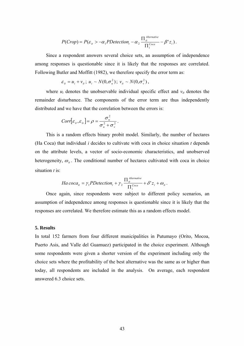
43

)'()( 21 iCocai

eAlternativit

tit zPDetectionPCropP βααε −Π

Π−−>= .

Since a respondent answers several choice sets, an assumption of independence

among responses is questionable since it is likely that the responses are correlated.

Following Butler and Moffitt (1982), we therefore specify the error term as:

itiit vu +=ε ; ),0(~ 2ui Nu σ ; ),0(~ 2

vit Nv σ ,

where ui denotes the unobservable individual specific effect and vit denotes the

remainder disturbance. The components of the error term are thus independently

distributed and we have that the correlation between the errors is:

[ ] 22

2

,vu

uisitCorr

σσσ

ρεε+

== .

This is a random effects binary probit model. Similarly, the number of hectares

(Ha Coca) that individual i decides to cultivate with coca in choice situation t depends

on the attribute levels, a vector of socio-economic characteristics, and unobserved

heterogeneity, itω . The conditional number of hectares cultivated with coca in choice

situation t is:

itiCocai

eAlternativit

tit zPDetectioncocaHa ωδγγ ++Π

Π+= ' 21 .

Once again, since respondents were subject to different policy scenarios, an

assumption of independence among responses is questionable since it is likely that the

responses are correlated. We therefore estimate this as a random effects model.

5. Results

In total 152 farmers from four different municipalities in Putumayo (Orito, Mocoa,

Puerto Asis, and Valle del Guamuez) participated in the choice experiment. Although

some respondents were given a shorter version of the experiment including only the

choice sets where the profitability of the best alternative was the same as or higher than

today, all respondents are included in the analysis. On average, each respondent

answered 6.3 choice sets.

44

Descriptive statistics

Table 5 presents the descriptive statistics of the variables used in the econometric

model. 43% of the farmers that participated in the stated preference study claimed to be

cultivating on average 1.32 hectares with coca. The profit of the alternative was on

average half the profit from coca. However, there is a large dispersion in the perceived

relative profitability of the alternative. Using the Mann-Whitney test, we cannot reject

the null hypothesis of equal distribution of the relative profitability among

municipalities at the 5% level, except for Puerto Asis with a significantly lower

perceived relative profitability of the alternative than Valle. We cannot reject the null

hypothesis of equal distribution of the relative profitability between coca and non-coca

farmers at the 1% significance level using the Mann-Whitney test except for Mocoa,

where non-coca farmers overestimate the profitability of the alternative compared with

coca farmers. Note that 17 participants think that the alternative is actually more

profitable than coca.

The average perceived risk of having the crops destroyed by authorities in 2005

was 3.88, which is relatively high on the 1-5 qualitative scale used. We find that there

are regional differences in the perceived risk of eradication. The average perceived risk

or eradication is significantly lower at the 5% level in Mocoa (2.75) and Orito (3.62)

compared with Puerto Asis (4.29) and Valle del Guamuez (6.5). This is consistent with

the fact that during 2004 and 2005, the number of sprayed hectares over total hectares

with coca was higher for Puerto Asis and Valle than for Mocoa and Orito. Interestingly,

coca and non-coca farmers within the same municipality have the same perceptions of

the eradication risk. Using the Mann-Whitney test, we cannot reject the null hypothesis

of equal distribution of the perceived risk between coca and non-coca farmers in each

municipality at the 1% significance level.

45

Table 5. Descriptive statistics

Variable Description Mean St Dev Perceived risk of eradication in 2005

Risk of having crops destroyed. 1 = very unlikely, 5 = very likely. 3.883 1.457

Relative profitability of alternative in 2005

Profit best alternative / Profit coca. 0.470 0.899

Experience Number of years cultivating coca. 5.964 5.295 Density coca in municipality

Number of hectares with coca over square kilometers in the municipality 2002-2003. 0.576 0.437

Legitimacy Index of acceptance of the law and the authorities. 1= Low, 5= High. 3.518 0.751

Level of moral development

Level of moral development. 0= Missing information, 1= Pre-conventionalist, 2= Conventionalist, 3 = Post-Conventionalist.

1.209 0.667

Missing level of moral development

= 1 if respondent was missing in Moral Judgment Test. 0.102 0.302

Atheist = 1 if respondent is atheist. 0.077 0.267 Protestant = 1 if respondent is Protestant. 0.124 0.329 Stated degree of trust Degree of trust. 1= not at all …..5= Very much. 3.057 1.238 Participation = 1 if respondent participates in a communitarian

organization. 0.599 0.490

Age Respondent age in years. 40.335 12.976 Female = 1 if respondent is female. 0.334 0.472 Educational level 0 = None, 1 = Basic primary, 2 = Primary complete, 3=

More than primary. 1.616 0.922

Risk attitude Respondent degree of risk aversion. Expressed in the degree of relative risk aversion. 3.271 3.514

Inconsistent risk Risk preference for prospect B and A changed more than once. 0.175 0.380

Transport Transport cost to the closest market in COL 2005. 2.731 2.186 Log hectares per capita

Natural logarithm of farm size per capita. 1.137 1.146

About one-third of the participants in the choice experiment were women, and the

average age of all participants was 40 years. The educational level of the participants

was very low: 40% had two years of education or less. In addition, the participants

tended to be very risk averse: 46% were classified as extremely or severely risk averse,

21% were classified as having intermediate or moderate risk aversion, and 23% were

risk neutral to risk loving. Most of the participants claimed to be Catholics (80%),

while around 12% declared to be Protestants.

Based on the Moral Judgment Test developed by Lind et al. (1985), 70% of the

respondents were classified as pre-conventionalists (the lowest level of moral

development), 26% as conventionalists (the intermediate level of moral development),

and the remaining 4% as post-conventionalists (the highest level of moral development).

These results are consistent with Aguirre’s (2002) findings on moral development in

Colombian teenagers. No significant differences at the 1% level were found in the level

46

of moral development between coca and non-coca farmers using the proportion test.

Due to time limitations, 10% of the participants in the choice experiment did not take

the Moral Judgment Test, but no significant differences were found between those who

took the test and those who did not with respect to age, gender, or educational level.

Econometric results

Table 6 presents the results of (1) the random effects probit model for the decision

whether or not to crop coca and (2) the random effects model for the conditional

decision on how many hectares to crop with coca. We report the marginal effects

evaluated at the sample mean. For the constant and the correlation coefficient, we report

the coefficients. For the continuous variables in the probit model, the marginal effect is

the marginal increase in the probability to crop coca associated with a marginal increase

in the corresponding variable. For dummy variables in the probit model, the marginal

effect is the increase in the probability to crop coca associated with a discrete change

from zero to one in the corresponding variable. For the linear model, the marginal

effects are simply the change in hectares used for coca.

The estimated correlation between the error terms across decisions, rho, is large

and highly significant in both models, which means that we cannot reject the random

effects model in favor of a more restrictive model with no correlation. Our results

support the traditional economic model of crime since increases in risk significantly

decrease both the probability to crop coca and the number of hectares with coca.

Similarly, increases in the profitability of the alternative reduce the likelihood to

cultivate coca and the number of hectares cultivated with coca. Our results also support

behavioral models of crime since other non-economic variables significantly affect the

likelihood to cultivate coca.

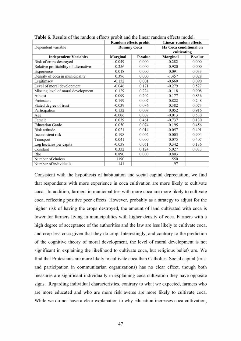
47

Table 6. Results of the random effects probit and the linear random effects model. Random effects probit Linear random effects Dependent variable Dummy Coca Ha Coca conditional on

cultivating Independent Variables Marginal P-value Marginal P-value

Risk of crops destroyed -0.049 0.000 -0.282 0.000 Relative profitability of alternative -0.256 0.000 -0.920 0.000 Experience 0.018 0.000 0.091 0.033 Density of coca in municipality 0.396 0.000 -1.457 0.028 Legitimacy -0.132 0.001 -0.660 0.090 Level of moral development -0.046 0.171 -0.279 0.527 Missing level of moral development 0.129 0.224 -0.118 0.908 Atheist -0.099 0.202 -0.177 0.836 Protestant 0.199 0.007 0.822 0.248 Stated degree of trust -0.039 0.086 0.382 0.073 Participation 0.132 0.008 0.052 0.916 Age -0.006 0.007 -0.013 0.530 Female 0.039 0.461 -0.737 0.130 Education Grade 0.050 0.074 0.195 0.456 Risk attitude 0.021 0.014 -0.057 0.491 Inconsistent risk 0.198 0.002 0.005 0.994 Transport 0.041 0.000 0.075 0.407 Log hectares per capita -0.038 0.051 0.342 0.136 Constant 0.332 0.124 5.027 0.033 Rho 0.890 0.000 0.803 Number of choices 1190 550 Number of individuals 141 97 Consistent with the hypothesis of habituation and social capital depreciation, we find

that respondents with more experience in coca cultivation are more likely to cultivate

coca. In addition, farmers in municipalities with more coca are more likely to cultivate

coca, reflecting positive peer effects. However, probably as a strategy to adjust for the

higher risk of having the crops destroyed, the amount of land cultivated with coca is

lower for farmers living in municipalities with higher density of coca. Farmers with a

high degree of acceptance of the authorities and the law are less likely to cultivate coca,

and crop less coca given that they do crop. Interestingly, and contrary to the prediction

of the cognitive theory of moral development, the level of moral development is not

significant in explaining the likelihood to cultivate coca, but religious beliefs are. We

find that Protestants are more likely to cultivate coca than Catholics. Social capital (trust

and participation in communitarian organizations) has no clear effect, though both

measures are significant individually in explaining coca cultivation they have opposite

signs. Regarding individual characteristics, contrary to what we expected, farmers who

are more educated and who are more risk averse are more likely to cultivate coca.

While we do not have a clear explanation to why education increases coca cultivation,

48

we think that the positive correlation between risk aversion and the likelihood to

cultivate coca can be explained by the higher perceived risk of the legal activity

associated with coca in terms of possibility to sell the product, price stability, and access

to productive credits. Finally, we find that coca cultivation is a result of poverty and

isolation from the markets. Respondents who live closer to the markets and who are

relatively richer in terms of larger land holdings are less likely to cultivate coca. Larger

land holdings allow compensation for the low return of legal products through extensive

production.

Validity test

The hypothetical choice experiments used to capture individual preferences may be

subject to multiple limitations. For instance, due to the illicit nature of coca farming,

participants would like to appear morally correct and therefore underreport cultivation.

In addition, participants may respond in ways they think the interviewer expects, or

their behavior could reflect strategic bias. Attempting to avoid the policy, participants

may for example falsify their preferences, reporting increases in coca cultivation as a

response to increases in the probability of eradication. They may also try to attract

compensation by overreacting at positive incentives, e.g., increases in the profit from

legal alternatives. Inconsistencies could of course also appear due to cognitive

limitations, fatigue effects, or simply random responses. Given the above limitation of

the methodology, we carry out a number of consistency tests. For example, a

respondent who states that he crops coca today should also state that he would crop if

the risk of eradication were reduced, or if the relative profitability of coca were

increased. Similarly, a farmer who states that he/she does not crop coca should not crop

if the risk were increased, or if the relative profit were reduced. Comparing the

responses within the experiment is referred to as an internal consistency test. Comparing

the responses in the experiment with the current behavior is referred to as an external

consistency test. In total, 18 respondents made at least one inconsistent choice in the

choice experiment, and 29 respondents made choices in the choice experiment that were

inconsistent with their actual behavior. However, many respondents were both

internally and externally inconsistent. Accounting for this, a total of 36 of the 152

respondents were inconsistent. Still, this is a non-negligible fraction of the respondents,

49

although we believe it is inevitable that any choice experiment will contain inconsistent

responses. We should also remember that the educational level of the respondents was

low, meaning that the respondents may not be deliberately acting in an inconsistent

manner. We estimated the model after removing inconsistent responses, and the results

were similar. The absolute values of marginal effects for the risk and profit attributes

are somewhat larger in the probit model and smaller in the linear model. The only

important difference is that the marginal effect of the profit attribute is insignificant in

the linear model. Most of the other control variables have the same sign and

significance, with some exceptions.

An alternative test on the quality of the data is to use the estimated model to

forecast the behavior and compare it with self-reported behavior. Therefore, using the

estimated coefficients in the model and considering the individual perceived risk of

eradication and profitability of the alternative relative to coca in 2003 and 2005, we

predict the decision to cultivate coca and the number of hectares to be cultivated for

each individual, and compare the findings with the self-reported behavior in both years.

Table 7 presents the self-reported and predicted proportion of farmers cultivating coca

and hectares cultivated with coca. Using the proportion test, we cannot reject the null

hypothesis of equality between the actual and predicted proportions of farmers who

cultivated coca in 2005, but we can reject the null hypothesis at the 1% significance

level for 2003. Using the t-test, we also reject the null hypothesis of equal means of

self-reported and predicted hectares with coca in 2003 and 2005. This indicates that

though the model does a fairly good job in predicting the proportion of coca farmers in

2005, its predictive power on the number of hectares is limited.

Table 7. Predicted and actual proportion of coca farmers and hectares with coca using individual data in 2003 and 2005 (standard deviations in parentheses.)

Proportion of coca farmers

Hectares with coca per farmer

P(crop) Ha Coca conditional on cultivating Year

Self-reported (1)

Predicted (2)

Self-reported (1)

Predicted (2)

2005 0.430 0.401 1.319b 1.870b (0.496) (0.491) (1.223) (1.118)

2003 0.665a 0.511a 1.649c 2.156c (0.473) (0.501) (1.343) (1.170)

a: Significant differences at the 10% level using the proportion test. b, c: Significant differences at the 10% level using the t-test.

50

Policy implications

From a policy perspective, it is important to analyze the effect of changes in the levels

of eradication and profitability of the alternative. Table 8 presents the raw results of the

choice experiment for the nine choice sets used. The share of respondents who would

crop coca and the conditional number of hectares that would be cultivated with coca

decrease significantly when the relative profitability of the alternative increases and

when the risk of having the crops destroyed increases. The exceptions are marked a, b,

and c. The effect on the proportion of farmers who would cultivate coca is non-linear

for increases in relative profits and risk of eradication. The proportion of coca farmers

decreases relatively less from the first to the second row (column) in Table 8 than from

the second to the third row (column). This non-linear effect suggests that alternative

development programs have a great potential to reduce coca cultivation if the profit

from the alternative is not too low. In the same way, eradication can only succeed

deterring coca cultivation with high levels of spraying.

Compared with self-reported behavior in 2005, we find that increasing the risk of

destroying the crops significantly does decrease the proportion of farmers who would

cultivate coca but does not significantly decrease the number of hectares cultivated with

coca. Further analysis reveals that about 10% of the farmers declared an intention to

start cultivation or to cultivate more hectares if the risk were to increase. This can be

interpreted either as risk seeking behavior, or as a threat to authorities. None of the

participants exhibits consistent risk-seeking behavior through all nine choice sets,

indicating that some strategic bias may be present in our sample.

51

Table 8. Proportions of people who would cultivate coca and number of hectares that would be cultivated at different levels of profitability and risk of detection. Standard deviations in parentheses.

Proportion Crop Coca Hectares cropped

Conditional on cultivating Zero risk

Lower risk Higher

risk Zero risk Lower risk Higher

risk

0.61 0.55a 0.39 4.03 2.79 2.02 Lower profitability of alternative than today (0.49) (0.5) (0.49) (4.18) (2.73) (2.14)

0.59 0.51a 0.31b 3.45 2.14 1.52c Same profitability of alternative as today (0.49) (0.5) (0.47) (4.33) (1.95) (1.39)

0.52 0.43 0.27b 3.1 2.09 1.76c Higher profitability of alternative than today (0.5) (0.5) (0.44) (3.66) (2.29) (1.86)

a,b: No significant differences at the 5% level using the proportion test. c: No significant differences at the 5% level using the Wilcoxon Test.

One way of comparing the relative effects of increases in the relative profit of the

alternative with the risk of having the crops destroyed is to look at elasticity. Table 9

reports the elasticities of eradication and alternative development estimated from our

econometric model. The risk level and relative profitability were evaluated at the 2005

mean and median values. In addition to the elasticities of the probability to crop and the

conditional amount of coca, we report the elasticity for the unconditional amount of

coca. The total marginal effect was calculated as:

[ ] [ ] [ ] [ ] [ ]1

0|0|

1=

∂>∂

+>∂

=∂=

∂∂

ii

iiii

i

i

i

i CropPxHaHaE

HaHaEx

CropPxHaE

, (6)

where Hai is the number of hectares dedicated to coca for farmer i, and xi is a

covariate.

Table 9. Elasticities for the two attributes in the choice experiment. Standard errors are in parentheses.

Probability Crop CocaP(Crop) Hectares with Coca

Ha Coca conditional on cultivating

Hectares total

-0.456 -0.464 -0.392 Risk of Eradication (0.050) (0.039) (0.029)

-0.074 -0.095 -0.105 Profit Alternative (0.011) (0.023) (0.013)

After controlling for non-economic factors that affect the decision to cultivate coca and

the number of hectares to be cultivated, we find that a 1% increase in the risk of having

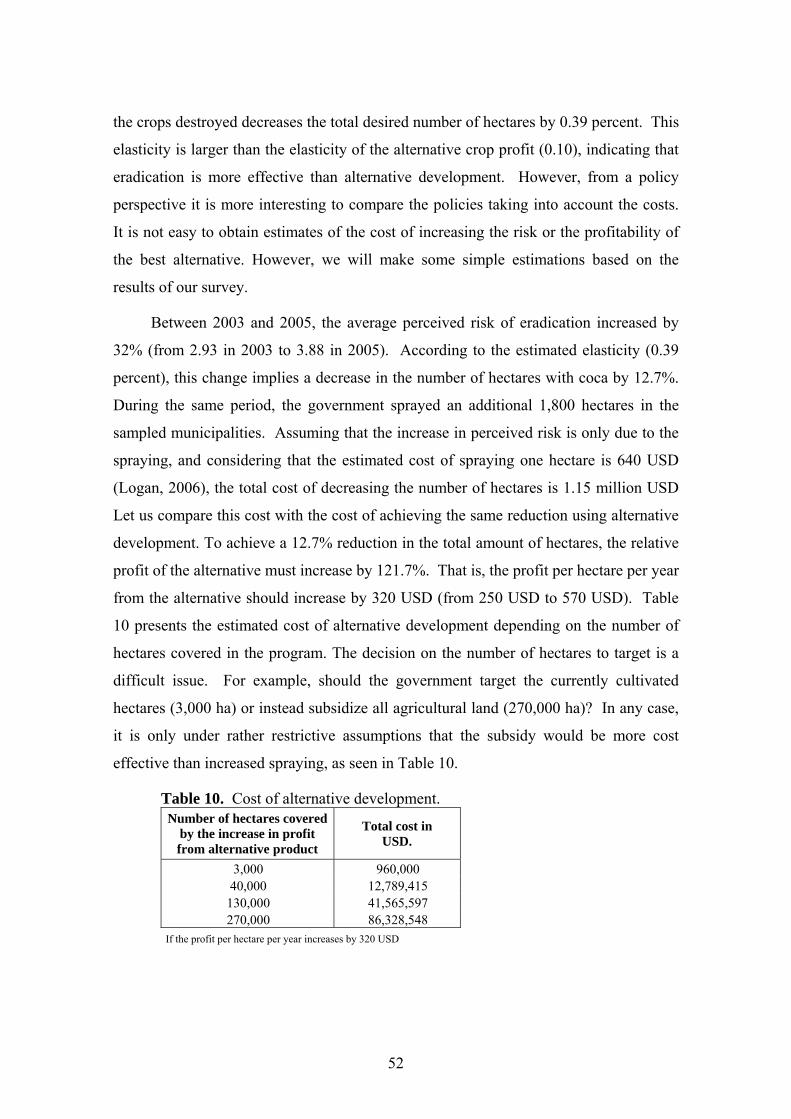
52

the crops destroyed decreases the total desired number of hectares by 0.39 percent. This

elasticity is larger than the elasticity of the alternative crop profit (0.10), indicating that

eradication is more effective than alternative development. However, from a policy

perspective it is more interesting to compare the policies taking into account the costs.

It is not easy to obtain estimates of the cost of increasing the risk or the profitability of

the best alternative. However, we will make some simple estimations based on the

results of our survey.

Between 2003 and 2005, the average perceived risk of eradication increased by

32% (from 2.93 in 2003 to 3.88 in 2005). According to the estimated elasticity (0.39

percent), this change implies a decrease in the number of hectares with coca by 12.7%.

During the same period, the government sprayed an additional 1,800 hectares in the

sampled municipalities. Assuming that the increase in perceived risk is only due to the

spraying, and considering that the estimated cost of spraying one hectare is 640 USD

(Logan, 2006), the total cost of decreasing the number of hectares is 1.15 million USD

Let us compare this cost with the cost of achieving the same reduction using alternative

development. To achieve a 12.7% reduction in the total amount of hectares, the relative

profit of the alternative must increase by 121.7%. That is, the profit per hectare per year

from the alternative should increase by 320 USD (from 250 USD to 570 USD). Table

10 presents the estimated cost of alternative development depending on the number of

hectares covered in the program. The decision on the number of hectares to target is a

difficult issue. For example, should the government target the currently cultivated

hectares (3,000 ha) or instead subsidize all agricultural land (270,000 ha)? In any case,

it is only under rather restrictive assumptions that the subsidy would be more cost

effective than increased spraying, as seen in Table 10.

Table 10. Cost of alternative development. Number of hectares covered

by the increase in profit from alternative product

Total cost in USD.

3,000 960,000 40,000 12,789,415

130,000 41,565,597 270,000 86,328,548

If the profit per hectare per year increases by 320 USD

53

Some warnings regarding this simplified analysis are relevant. We are comparing

policies based only on financial cost, but if we consider the non-economic cost of

eradication such as water contamination, destruction of natural areas, productivity losses

in soils, and negative health effects, then another picture could emerge. To our

knowledge, no previous studies have quantified the environmental impact of

eradication. From a distributional perspective, it could be preferable to give monetary

incentives to the farmers living in these regions, as they are relatively poor compared to

the national average. Moreover, alternative development could have long-term effects

not achieved through eradication. When farmers decide to substitute or reduce coca

cultivation, they implicitly accept a lifestyle change and consequently become more

likely to avoid coca cultivation in the future.

6. Conclusions

This paper contributes to the literature evaluating the effectiveness of policies against

coca cultivation. We found that increases in the risk of eradication and increases in the

relative profit of the alternative crops reduce the proportion of coca farmers and the

number of hectares with coca. These results support Becker’s (1968) model of crime. In

addition, our results support behavioral models of crime as other non-economic

variables also affect coca cultivation. Experience, density of coca in the municipality,

religion, and legitimacy of the authorities were significant in explaining coca

cultivation. Coca cultivation is also due to marginality and poverty. While our

econometric model gives an accurate estimative of the proportion of farmers who self-

report cultivating coca, the predictions on the number of hectares are less accurate.

From a policy perspective, we found that the risk of eradication elasticity is

higher than the relative profitability elasticity, suggesting that eradication is more

effective than alternative development. From an efficiency point of view, taking the

costs of the two policies into account, the difference between them is even stronger:

spending the money on increased eradication risk is likely to have a larger effect on the

amount of coca than spending the money on alternative development.

In our analysis, we have ignored the dynamic characteristics of coca cultivation

assuming that farmers independently decide how to allocate land in each choice set.

54

However, since coca plants are perennial, the amount of land cultivated with coca

depends on past decisions and economic conditions. In addition, we asked farmers for

the perceived risk of eradication assuming that they were able to imagine how the

situation would be if the risk were higher or lower, although this task may be too

demanding considering our low-educated sample. This study contributes to the limited

body of literature evaluating anti-drug policies against coca cultivation and, despite its

multiple limitations; we do consider it to be relevant for policy purposes.

55

7. References Aguirre, Eduardo. 2003. “Juicio moral presente en delincuentes menores” Estudio para la Alcadia mayor

de Bogota. Universidad Nacional de Colombia. Akerlof, George. 1997. “Social Distance and Social Decisions” Econometrica. 65 (September): 1005-

1028. Allingham, Michael G. and Agnar Sandmo. 1972. “Income tax evasion: A theoretical analysis,” Journal

of Public Economics. 1 (November): 323-338. Alpizar, Francisco, Fredrik Carlsson and Peter Martinsson. 2003. “Using Choice Experiments for Non-

Market Valuation.” Economic Issues. 8(June):83-110. Andreoni, James, Brian Erard and Jonathan Feinstein. 1998. “Tax Compliance.” Journal of Economic

Literature. 36 (June): 818-860. Becker, Gary. 1968. "Crime and Punishment: An Economic Approach," Journal of Political Economy. 76

(March-April): 169-217. Binswanger, Hans P. 1980. “Attitude towards risk: experimental measurement in rural India” American

Journal of Economics. 62(August): 395-407. Bowles, Samuel and Herbert Gintis. 1998. “The Moral Economy of Communities: Structured Populations

and the Evolution of Pro-Social Norms.” Evolution and Human Behavior. 19 (1): 3-25. Butler, J.S. and Robert Moffit. 1982. “A Computationally Efficient Quadrature Procedure for the One

Factor Multinomial Probit Model.” Econometrica. 50 (May): 761-764. Calvó-Armengol, Antoni. and Yves Zenou. 2004. “Social Networks and Crime Decisions: The role of

social structure in facilitating delinquent behavior.” International Economic Review. 45 (August): 939-958.

Cameron, Samuel. 1988. “The economics of crime deterrence: A survey of Theory and Evidence”. Kyklos. 41(May):301-323.

Carvajal, Maria Paula. 2002 “Factores explicativos de la presencia de cultivos ilícitos en los municipio de Colombia” Dissertation paper to opt to the title in the Master program in environmental economics. CEDE- Universidad de los Andes. Bogotá, Colombia.

Cohen, Mark A. 1999. “Monitoring and Enforcement of Environmental Policy”. InTietenberg, Tom, Henk Folmer (Eds.) International Yearbook of Environmental and Resource Economics.

Díaz, Ana María and Fabio Sanchez. 2004. “Geography of Illicit Crops and Armed Conflict in Colombia” Documento CEDE 2004-18 No.1657-7191. March

Ehrlich, Issac. 1973. “Participation in illegitimate activities: a theoretical and empirical investigation” Journal of Political Economy. 81 (May-June): 521-565.

Eide Erling, Paul Rubin and Joanna Shepherd. 2006. “Economics of crime.” Now Publishers Inc. Eisenhauer Joseph. 2004. “Economic Models of Sin and Remorse: Some Simple Analytics.” Review of

Social Economy, 62(June): 201-219. Elster, Jon. 1989. ‘‘Social Norms and Economic Theory’’ Journal of Economic Perspectivas. 3

(Autumn): 99-118. Feld, Lars and Bruno Frey. 2005. “Tax Compliance as the Result of a Psychological Tax Contract: The

Role of Incentives and Responsive Regulation.” Paper presented at the Annual Meeting of European Public Choice Society. Durham (UK)

Feld, Lars and Jean Robert Tyran. 2002. “Tax evasion and voting: an experimental analysis”. Kyklos. 55 (May): 197-221.

Freeman, Richard. 1999. “The economics of Crime” In O. Ashenfelter & D. Card (ed.) Handbook of Labor Economics, Chapter 52: 3529-3571.

Frey, Bruno. 1997. “Not just for the money: an economic theory of personal motivation.” Edward Elgar Publishing Cheltenham UK.

Frey, Bruno and Benno Torgler. 2004. “Taxation and conditional cooperation” Working paper 2004/7. Institut d’Economia de Barcelona. Centre de recerca en federalism fiscal I economia regional.

Garoupa, Nuno. 2003. “Crime and Social Norms.” Portuguese Econonomic Journal. 2 (December): 131-144.

Glaeser, Edward L. Bruce Sacerdote and Jose A. Scheinkman. 1996. “Crime and Social Interactions.” Quarterly Journal of Economics. 111 (May): 508–48.

Hausman, Daniel and Michael. McPherson. 1993. ‘‘Taking Ethics Seriously: Economics and Contemporary Moral Philosophy.’’ Journal of Economic Literature. 31 (June): 671-731.

Kennedy, Michael, Peter Reuter and Kevin Riley. 1993. “A Simple Economic Model of Cocaine Production.” Mathematical and Computer Modelling, 17 (2): 19-36

56

Kohlberg, Laurence. 1969. “Stage and sequence: The cognitive developmental approach to socialization.” In: D. Goslin, ed., Handbook of socialization theory and research. Chicago: Rand McNally, pp. 347-480.

Lind, George, Hans A. Hartmann and Roland Wakenhut (Eds). 1985. Moral Development and the Social Environment Studies in the Philosophy and Psychology of Moral Judgment and Education.

Logan, Sam. 2006. “Hydras, Balloons, Wasted Money in los Andes”. ISN Security Watch in Buenos Aires.

Louviere, Jordan, David Hensher and Joffre Swait. 2000. “Stated Choice Methods.”. Cambridge: Cambridge University Press.

Moreno Sanchez, Rocio, David S. Kraybill and Stanley R. Thompson. 2003. “An econometric analysis of coca eradication policy in Colombia.” World Development. 31 No. 2: 375-383.

Moya, Andrés. 2005 “Impacto de la erradicación forzosa y el desarrollo alternativo sobre los cultivos de coca.” Dissertation paper. Universidad de los Andes. Bogotá, Colombia.

ONDCP. 2006. “The economic cost of drug abuse in the USA 1992-2002.” Office of National Drug Control Policy. Washington. United States of America.

Posner, Richard. 1997. “Social Norms and the Law: an economic approach.” American Economic Review 87 (May): 365-369.

Riley, Kevin. 1991. “Snow Job?: The efficacy of Source Country Cocaine Policies.” Dissertation. Rand Graduate School. RGSD-102. Santa Monica.

Sutinen, Jon and K. Kuperan. 1999. "A Socio-Economic Theory of Regulatory Compliance." International Journal of Social Economics. 26 (1/2/3): 174-193.

Tabares, Elizabeth and Ramón Rosales. 2004. “Políticas de control de oferta de coca: La zanahoria y el garrote.” Documento CEDE 2005-10. Universidad de los Andes. Bogotá, Colombia.

Torgler, Benno. 2002. “Speaking to the theorist and searching for the facts: tax morale and tax compliance in experiments.” Journal of Economic Surveys. 16 (December): 657-83.

Trivedi, Viswanath Umashanker, U., Mohamed Shehata and Stuart Mestelman. 2005. “Attitudes incentives and tax compliance.” Canadian Tax Journal. 53 (1): 29-61. Tyler, Tom R. 1990. Why People Obey the Law. New Haven, CT: Yale Univ. Press. Tyran Jean Robert and Lars Fehr. 2004. “Achieving compliance when legal sanctions are non-deterrent”

Scandinavian Journal of Economics. 101 (March): 135-156. UN. 1961. “Single Convention on Narcotic Drugs.” United Nations. UN. 1971. “Convention on Psychotropic Substances. ” United Nations. UN. 1988. “United Nations Convention against Illicit Traffic in Narcotic Drugs and Psychotropic

Substances.” United Nations. UNDCP. 2006. “World Drug Report.” United Nations Office on Drugs and Crime.

57

Carrots or sticks to reduce coca cultivation?

- A framed field experiment with farmers in Colombia #

Marcela Ibanez∗ and Peter Martinsson Department of Economics,

Göteborg University, Sweden

Abstract

We investigate the effect of different combinations of carrot and stick policies on coca

investment among farmers in coca growing areas in Colombia by applying a public bad

experiment that mimics coca cultivation. The experiment indicates that subjects are

more responsive to changes in the relative profit of cattle farming than to changes in the

probability of coca eradication. Moreover, we find evidence that behavior in the

experiment is consistent with self-reported behavior, namely that in addition to

economic incentives, social norms, religious beliefs and poverty also explained coca

investments

Keywords: Coca; Colombia; Experiment; Public Bad.

JEL classification:, C93, D62, K42

# We would like to thank Ali Ahmed, Alpaslan Akay, Fredrik Carlsson, Håkan Eggert, Martin Kocher, Katarina Nordblom and Matthias Sutter, participants at the ESA meeting 2006 in Nottingham, the ESA meeting in Tucson 2006, the First Nordic conference on Behavioral Economics in Oslo, as well as seminar participants at Universidad de los Andes and Göteborg University for their comments. We are very thankful for the hospitality and help from people at Universidad de los Andes, especially Juan Camilo Cardenas, during our fieldwork. Financial support from the Swedish Agency for International Development Cooperation (Sida) to the Environmental Economics Unit at Göteborg University and from Vetenskapsrådet (Swedish Research Council) is gratefully acknowledged. ∗ Department of Economics, Göteborg University, Box 640, SE 405 30 Göteborg, Sweden, e-mail: Marcela.Ibanez@economics.gu.se (corresponding author).

58

1. Introduction

The “War on Drugs” was initiated by the US president Richard Nixon who labeled drug

abuse as “America's public enemy number one”. In order to combat cocaine production

a strong policy to reduce coca cultivation was introduced in Colombia, the world's

leading producer of coca (the base for cocaine) (DNE, 2005). The policy against coca

cultivation use two main strategies: (i) a stick policy whereby coca plants are eradicated

by aerial fumigation as well as by pulling up plants manually (ii) a carrot policy that

aims to increase the relative profit between non-coca agricultural activities and coca

cultivation by implementing alternative development programs (e.g. investment in

infrastructure, subsidized loans, technological advice).17 Although one billion dollars

has been spent annually on campaigns against coca cultivation, especially on aerial

fumigation, little is known about the effects of eradication, alternative development

programs or the motivational factors behind coca cultivation.

One of the problems encountered in the analysis of coca cultivation and the

evaluation of how effective different policies against coca cultivation are, is the lack of

data at the individual level. The few empirical studies that do exist have used data at the

municipal level to investigate the effectiveness of different supply control measures on

coca cultivation. The overall results from these studies show that alternative

development programs have had a significant impact on reducing coca cultivation, but

that aerial fumigation programs have not (e.g.; Carvajal, 2002; Moreno et al, 2003; Díaz

and Sánchez, 2004; Moya, 2005 and Tabares and Rosales). However, revealed data does

not provide information on behavior for policy levels that are outside the ranges that

have been used historically. One alternative for obtaining individual information on

coca investment decisions at different levels of alternative development (carrots) and

eradication (sticks) is to use what Harrison and List (2004) classified as a framed field

experiment. The basic idea of the framed field experiment is to impose a controlled

environment in a situation that is not unnatural for participants. Using a framed

experiment with subjects who are faced with cultivation decisions in real-life has the

added benefit of allowing motivational factors behind coca investments to be included

17 In recent years alternative development has also used voluntary agreements that consist of monetary subsidies in exchange for an undertaking not to cultivate coca (DNE, 2005).

59

in the analysis (e.g. morality, religious beliefs, poverty). We use complementary survey

information to capture those factors.18

The objective of this paper is to investigate how the decision to invest in coca

changes when the relative profit from the alternative development programs (carrot

policies) and the probability of eradication (stick policies) varies using a framed field

experiment that mimics real-life situations. The subjects of our study were farmers

living in Putumayo, a region in Colombia with a long tradition of coca cultivation. We

also use additional survey information in order to compare experimental and self-

reported behavior and interpret the results in terms of policy implications.19

The use of experiments to capture compliance is not new, having mostly been

applied to studying the effects of the severity and probability of punishment (e.g. Alm

et. al. 1992a, 1992b, Anderson and Stafford, 2003; Trivedi et al., 2003, 2005, Cardenas

et al., 2000) but disregarding the effects of positive and negative incentives. Our

research contributes to the limited experimental literature on carrots and sticks, when

both mechanisms are exogenous. For example Sefton et al. (2000) find that both

rewards and sanctions increase cooperation in a public goods game but only sanctions

are effective in sustaining cooperation. Sutter et al. (2006) find that endogenously

chosen institutions, whether they imply positive or negative incentives, increase

cooperation more than when they are exogenously imposed. However, none of the

above papers consider mixing positive and negative incentives that are imposed

exogenously. This paper also contributes to the literature on the relationship between

behavior in the lab and in the field (e.g. Barr and Serneels, 2004; Cardenas and Ostrom,

2004; Carpenter and Seki, 2004; Levitt and List, 2007; Karlan, 2006: Potters and van

Winder, 2000) by investigating the motivational factors behind coca investments in both

settings.20

18 For example, Eckel and Grossman (1996) and Loewenstein (1999) argue that a non-neutral framing is needed in experiments where social context plays an important part in the problem under investigation . Moreover, in a sample with a low level of education, as in our case, a non-abstract description also has the benefit of making the task less complex. 19 In our study, we focus on the mechanisms available for Colombian authorities to reduce coca cultivation by using exogenous institutions, and hence we do not consider the effect of endogenous mechanisms of social control (e.g. Ostrom et al., 1992; Fehr and Gächter, 2000). In addition, we do not consider the scenario of legalizing drugs as it is politically unfeasible. 20 A growing body of literature that indicates that motivational factors as social norms (e.g. Glaeser et al., 1996; Akerlof, 1997; Calvó and Zenou, 2004, Garoupa 2003), morality (Eisenhauer, 2004, Sutinen and Kuperan 1999, Hatcher et al. 2000) and acceptance by the authorities (Tyler, 1990, Kuperan and Sutinen, 1998; Feld and Tyran, 2002) affect compliance with the law.

60

The rest of the paper is organized as follows. In section 2 we describe the main

features of coca cultivation in the field and in section 3 we present our experimental

design and predictions. Section 4 describes the procedure used and Section 5 presents

our results. Finally, Section 6 concludes the paper.

2. The field context

The Department of Putumayo in southern Colombia is a region with one of the longest

traditions of coca cultivation in the country to the extent that, in 2000, two fifths of

Colombia’s coca-growing areas were located there. Following a strong eradication

campaign during 2002 and 2003, and also as the result of the establishment of

Voluntary Agreements of Substitution, the number of coca-growing areas dropped.

Even so, by 2005 one tenth of Columbia’s coca-growing areas were still located in this

department. Other agricultural activities in Putumayo are cattle farming and the

cultivation of plantain, cassava and tropical fruits. Depending on the soil condition and

technology applied, the monetary profit from investments in non-coca activities are

approximately 20% to 85% of the profit from coca cultivation (Forero et al., 2002). In

the survey that we conducted parallel to the experiment, farmers stated an average profit

of 1,402 USD per hectare of coca compared with an average profit of 391 USD for

cattle farming in 2005, which implies a relative profit for cattle farming of 0.28. In

contrast, the relative profit was 0.14 in 2003. This low relative profit reflects the rural

location of Putumayo, where farmers have few possibilities to sell their products.

Following the 1961 ”International Convention on Narcotics and Drugs”, the

cultivation, processing and trafficking of coca was prohibited in Colombia (UN, 1961).

As a response to the increase in coca production during the 90s, the Colombian

authorities approved the use of aerial spraying to destroy coca fields and more recently

implemented the manual destruction of coca plants. Between 1999 and 2005 the number

of sprayed hectares in Putumayo was 210,244 with 200,004 hectares being dedicated to

coca- cultivation. Considering that in order to eradicate one hectare of coca it is

necessary to spray 3 to 8 hectares to exterminate the plants completely, the probability

of eradication is estimated to be between 13% and 35% (DNE, 2006).21 While the law

21 The probability of eradication is estimated as the number of hectares destroyed divided by the total number of hectares cultivated with coca. The number of destroyed hectares is estimated by dividing the

61

prescribes imprisonment for cultivating coca, this is rarely enforced since it is difficult

to capture the owners of the fields, thus the supply control focuses on eradication.

Another characteristic of coca cultivation is that it generates negative

externalities for the society. In addition to the health and social problems from coca and

cocaine consumption per se, the pesticides and chemicals that are used in coca

cultivation and the processing of coca leaves into cocaine contaminate the water and

soil. In response to increased eradication and poor soil quality on old plots, coca

farmers often relocate their coca plantations into forested areas where trees must be cut

down which in turn often leads to erosion problems in the future. Another negative

effect is caused by the spraying since the chemicals use to eradicate the coca often hit

non -targeted areas such as non-coca crops, water sources and occasionally residential

areas. In addition, in the backwash of coca cultivation, there is increased violence from

disputes between armed groups over the control of coca intermediation. Moreover, the

increased income due to coca cultivation has also led to a larger proportion of people

carrying weapons, increased numbers of robberies that are sometimes fatal, as well as

an increased level of alcohol consumption due to increased income. Perez et al. (2002)

estimated that the average annual cost of illicit drugs in Colombia was about one billion

dollars or the equivalent to 1% of the GDP.

3. Experimental design

In the experiment we used a framed public bad experiment in which we form random

groups of five farmers. Each farmer is endowed with 10 tokens that represent the

amount of land, labor and capital that are available to them to invest in agricultural

activities and their task is to decide how many tokens to invest in coca cultivation and

cattle farming respectively. The three key features of coca cultivation included in the

public bad experiment are: (i) coca production is more profitable than cattle farming, (ii)

there is a probability that the coca plants will be eradicated by the authorities, and (iii)

coca production generates negative externalities (see the protocol used in the

experiment in Appendix A).

In the experiment, each unit invested in coca cultivation yields a return of one,

while investment in cattle farming gives a return of less than one, mimicking the fact number of sprayed hectares by the number of times that one hectare needs to be sprayed in order to be destroyed.

62

that investment in coca cultivation yields a higher profit than investments in cattle

farming. Based on observations from real-life and likely future levels, we included the

following three levels of relative profits between cattle farming and coca cultivation;

0.2, 0.44 and 0.68.

However, investment in coca cultivation is a risky decision since the plantation

can be detected and subsequently eradicated. Since successful eradication is not certain,

we introduce the probability of successful eradication. We applied the following three

levels of successful eradication: 0%, 10% and 30%. These levels correspond to real life

values. If coca plants are sprayed, farmers collect and process the leaves to sell them,

but the coca plantation is lost, and the sprayed land cannot be used for any crops in the

near future. For each unit invested in coca when eradication is successful, the resulting

effect is a loss of income of 1.2 tokens in the experiment.22 We keep the loss of income

from eradication constant as the authorities can not usually do more harm than

destroying the coca fields.

The third specific feature of coca cultivation is that it generates negative

externalities such as environmental damage and social problems that affect everyone in

the community.23 These effects were included in the experimental design by making

each unit of coca cultivation generated by any one member reduce the income by 0.17

for every person in the group including the one who made the investment.24 To explain

these effects to the subjects, we stated that these costs relate to the increased violence

and environmental problems that arise from increased coca production. As we used

three levels of probability for eradication and three levels of relative profit, each farmer

participated in 9 one-shot experiments. The expected pay-off for subject i can then be

expressed as

)2.117.0)10(()17.0)10(( )1(5

1

5

1i

iiii

iiiii cccacpccacp −−−++−−+−= ∑∑

==

π ,

where p is the probability of eradication, ci is the amount invested in coca cultivation

and a is the relative profit. The parameters included in the experiment ensure a social 22 What we framed as a payment could also be phrased as a fine. The effect is the same, but to replicate reality in Colombia, it is better to use the wording payment. 23 The best alternative, cattle farming, also has negative environmental impacts related with soil erosion and deforestation, but our main interest is to capture the effect of the illegality of coca. 24 It would also be of interest to investigate the effect of different magnitudes of loss of income and negative externality, but we preferred to keep the design as simple as possible given that it is already rather complicated with 9 different decisions.

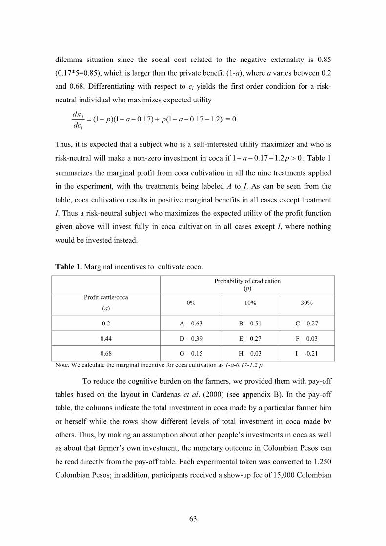
63

dilemma situation since the social cost related to the negative externality is 0.85

(0.17*5=0.85), which is larger than the private benefit (1-a), where a varies between 0.2

and 0.68. Differentiating with respect to ci yields the first order condition for a risk-

neutral individual who maximizes expected utility

)2.117.01()17.01)(1( −−−+−−−= apapdcd

i

iπ = 0.

Thus, it is expected that a subject who is a self-interested utility maximizer and who is

risk-neutral will make a non-zero investment in coca if 02.117.01 >−−− pa . Table 1

summarizes the marginal profit from coca cultivation in all the nine treatments applied

in the experiment, with the treatments being labeled A to I. As can be seen from the

table, coca cultivation results in positive marginal benefits in all cases except treatment

I. Thus a risk-neutral subject who maximizes the expected utility of the profit function

given above will invest fully in coca cultivation in all cases except I, where nothing

would be invested instead.

Table 1. Marginal incentives to cultivate coca.

Probability of eradication (p)

Profit cattle/coca

(a) 0% 10% 30%

0.2 A = 0.63 B = 0.51 C = 0.27

0.44 D = 0.39 E = 0.27 F = 0.03

0.68 G = 0.15 H = 0.03 I = -0.21

Note. We calculate the marginal incentive for coca cultivation as 1-a-0.17-1.2 p

To reduce the cognitive burden on the farmers, we provided them with pay-off

tables based on the layout in Cardenas et al. (2000) (see appendix B). In the pay-off

table, the columns indicate the total investment in coca made by a particular farmer him

or herself while the rows show different levels of total investment in coca made by

others. Thus, by making an assumption about other people’s investments in coca as well

as about that farmer’s own investment, the monetary outcome in Colombian Pesos can

be read directly from the pay-off table. Each experimental token was converted to 1,250

Colombian Pesos; in addition, participants received a show-up fee of 15,000 Colombian

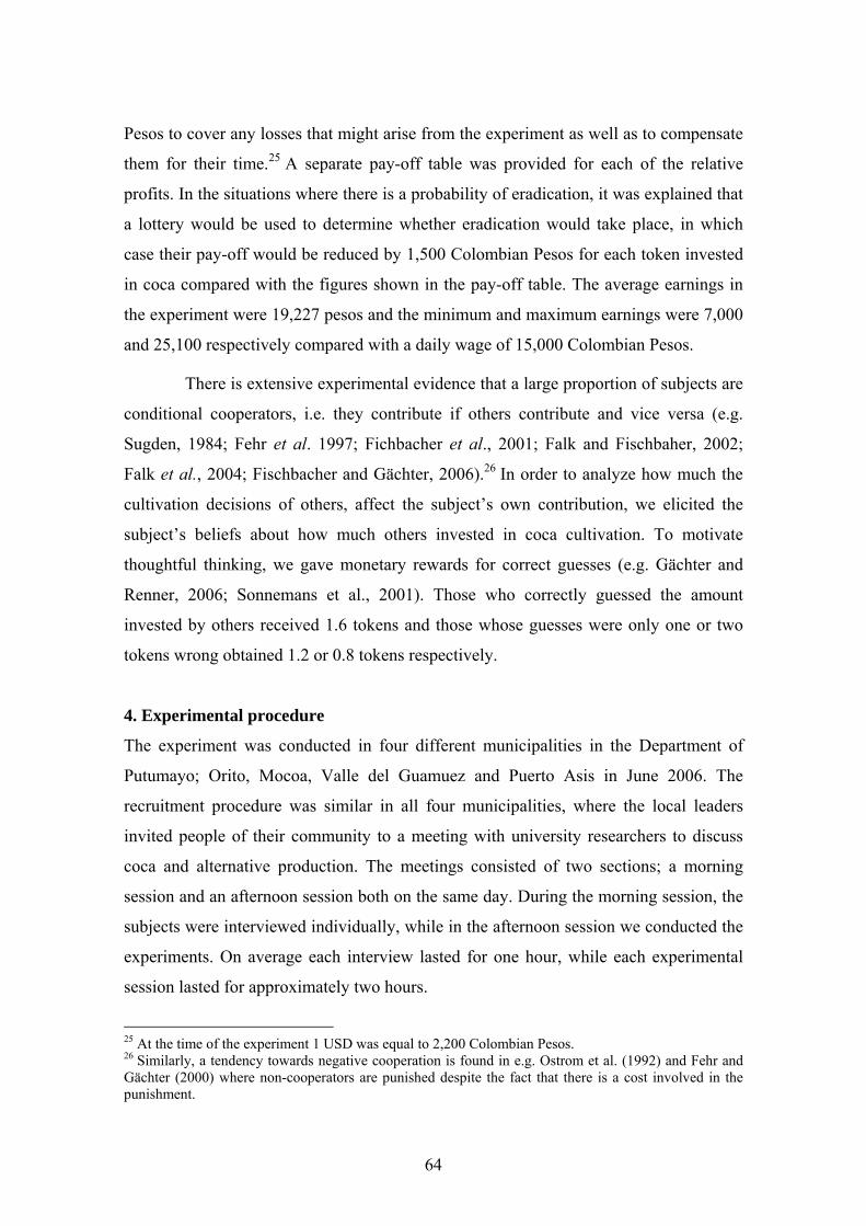
64

Pesos to cover any losses that might arise from the experiment as well as to compensate

them for their time.25 A separate pay-off table was provided for each of the relative

profits. In the situations where there is a probability of eradication, it was explained that

a lottery would be used to determine whether eradication would take place, in which

case their pay-off would be reduced by 1,500 Colombian Pesos for each token invested

in coca compared with the figures shown in the pay-off table. The average earnings in

the experiment were 19,227 pesos and the minimum and maximum earnings were 7,000

and 25,100 respectively compared with a daily wage of 15,000 Colombian Pesos.

There is extensive experimental evidence that a large proportion of subjects are

conditional cooperators, i.e. they contribute if others contribute and vice versa (e.g.

Sugden, 1984; Fehr et al. 1997; Fichbacher et al., 2001; Falk and Fischbaher, 2002;

Falk et al., 2004; Fischbacher and Gächter, 2006).26 In order to analyze how much the

cultivation decisions of others, affect the subject’s own contribution, we elicited the

subject’s beliefs about how much others invested in coca cultivation. To motivate

thoughtful thinking, we gave monetary rewards for correct guesses (e.g. Gächter and

Renner, 2006; Sonnemans et al., 2001). Those who correctly guessed the amount

invested by others received 1.6 tokens and those whose guesses were only one or two

tokens wrong obtained 1.2 or 0.8 tokens respectively.

4. Experimental procedure

The experiment was conducted in four different municipalities in the Department of

Putumayo; Orito, Mocoa, Valle del Guamuez and Puerto Asis in June 2006. The

recruitment procedure was similar in all four municipalities, where the local leaders

invited people of their community to a meeting with university researchers to discuss

coca and alternative production. The meetings consisted of two sections; a morning

session and an afternoon session both on the same day. During the morning session, the

subjects were interviewed individually, while in the afternoon session we conducted the

experiments. On average each interview lasted for one hour, while each experimental

session lasted for approximately two hours.

25 At the time of the experiment 1 USD was equal to 2,200 Colombian Pesos. 26 Similarly, a tendency towards negative cooperation is found in e.g. Ostrom et al. (1992) and Fehr and Gächter (2000) where non-cooperators are punished despite the fact that there is a cost involved in the punishment.

65

The experimental session consisted of five stages. First, the instructions of the

modified public bad experiment were read aloud to the subjects (see Appendix A),

followed by several examples and individual exercises. To check for subjects’

understanding of the experiment an enumerator accompanied them verifying that they

understood their task. Then, the subjects simultaneously decided how much they wanted

to invest in coca and how much they expected others to invest in each of the nine

treatments, where the probability of eradication and relative profits varied as described

above. In the third stage, we used a lottery, where each treatment had the same chance

of being selected, to decide randomly which of the nine treatments would be paid by. If

a treatment with a positive probability of eradication was selected, then a second lottery

was used to determine if successful eradication took place. The outcomes from these

two lotteries are common to everyone. This mimics the actual situation since both

relative profits and successful eradication are normally the same for people living close

to each other. Finally, all subjects were paid privately using checks made payable to

them in the local store. 27 Afterwards, following similar procedures as applied by

Cardenas and colleagues (e.g. Cardenas et al., 2000), there was a group discussion on

the experiment and its similarity to real life.

The morning sessions consisted of individual interviews. The interviews were

anonymous and in order to encourage honest answers we did not ask names, addresses

or any other identifying information. To match survey and experimental information we

used identification numbers with the date of birth or any other number that they could

remember. The survey consisted of a battery of standard questions on socioeconomic

characteristics and some specialized questions for our research relating to how much

coca they cultivated in 2003 and 2005, risk preferences, moral development and

legality, or acceptance of the authorities and the law.

Risk preferences were elicited by a hypothetical risk experiment based on the

design in Binswanger (1980). In this design, subjects were asked to choose between a

safe alternative and an alternative with two outcomes one of which had a lower pay-off

than the safe alternative and the other a higher pay-off. The probability of selecting each

of the outcomes was 50%. Each farmer was asked to make five such choices, where in

each subsequent choice presented to them both the expected pay-off and its variance 27 It would have been better to use cash, but for practical reasons we preferred to avoid carrying large amounts of cash.

66

increased in the risky alternative. The point at which the subject chose to switch from

the risky to the safe alternative allowed us to calculate the degree of risk aversion,

where we assumed a constant partial relative risk aversion utility function.

According to Colby and Kohlberg (1987), the individual level of moral

development affects law compliance.28 To determine the level of moral development,

the Moral Judgment Test developed by Lind et al. (1985) was used. In the test, subjects

have to select statements that best represent their views about the actions taken in two

dilemmas; euthanasia and protection of workers rights. Based on the answers, the

subjects can be divided into three levels of moral development; (i) pre-conventionalist

(moral actions are motivated by the fear of punishment or by self-interest), (ii)

conventionalist (motivated by the intention to please or help others or to fulfill social

rules) and (iii) post-conventionalists (motivated by concepts of justice and rights or

from universal principles).

According to Tyler’s (1990) theory of procedural justice, legitimacy of the

authorities plays a crucial role in legal compliance. The fairness of the law and the

regulators of the law, the efficacy in which that law is enforced and the possibility of

participating in decisions regarding its regulation have all been identified as factors that

affect law compliance behavior.29 To capture the effect of legality we constructed an

index that captures the level of agreement with statements regarding respect towards the

law, the fairness of authorities executing the law and participation of the community in

defining substitution alternatives.

5. Results

In total, 293 farmers participated in the interviews while 164 of them also took part in

one of the 13 organized experimental sessions. We test for attrition between the survey

and the experiment using the proportion test and the Wilcoxon ranksum test. We cannot

reject the null hypotheses of an equal proportion of coca farmers or of an equal number

28 Empirical evidence supporting this theory is provided by Trivedi et al. (2003) and Kuperan and Sutinen (1998). Another study that reports a positive effect of morality is Offerman et al (1996). 29 Participation in fixing regulations by voting or by communication has been identified as a factor that positively affect legal compliance (e.g. Cardenas et al., 2000; Cardenas 2004, 2005; Murphy and Cardenas., 2004; Ostrom et al., 1992; Tyran and Feld, 2002; Feld and Tyran, 2002). In addition, Fortin et al. (2003) and Trivedi et al. (2003) find that the fairness of the rule affects compliance while Nadler, (2005) concludes that the perceived injustice of authorities can also affect general compliance. Galbiati et al. (2005) find that imposing the obligation to comply affects the average level of contributions.

67

of hectares of coca cultivated at 5% significance level between those who only took part

in the interview and those who took part in both the interview and the experiment using

the proportion test and the Wilcoxon ranksum test respectively. Whether our sample is

representative for the populations of farmers living in these areas is difficult to evaluate,

but when compared with official statistics at the municipality level (DNE, 2006), the

proportion of plots larger than 3 hectares in our sample (2.73%) is not significantly

different at 5% level from the official reports (3.9%) using the proportion test.

5.1. Descriptive statistics

The descriptive statistics for the participants in the experiment are presented in Table 2.

The second column presents the descriptive statistics for the overall population and the

third and fourth columns present the same information but separated between coca and

non-coca farmers, respectively. We test the null hypothesis of equal distribution of the

variables between coca and non-coca farmers separately for each of the variables, where

the significance levels are shown in the last column of the table. As presented in the last

column of table 2, we reject the null hypothesis in some cases, most notably in

education levels, years of coca cultivation, participation in community organizations

and in statements about obligation to comply.

In Table 3 we present the summary statistics of investments in coca for the nine

treatments used in the experiment. The rows represent the different relative profits of

cattle farming compared with coca cultivation while the columns represent the different

probabilities of eradication used in the experiment. We present the results separately for

the average total investment in coca, the proportion of subjects with a non-zero

investment in coca, and the average investment conditional on non-zero investment.

Using the Wilcoxon sign rank test, we reject the null hypothesis that average investment

in treatments A to H is equal to 10 tokens (the expected amount to be invested by a risk-

neutral subject) at 1% significance level in separate tests. Similarly, we also reject the

null hypothesis that subjects invested zero tokens in treatment I. The latter indicates that

factors other than pure selfishness explain individual behavior.

68

Table 2. Descriptive statistics.

Variable Overall mean Non-Coca Farmers Coca Farmers

n = 141 n = 81 n = 60 Ho: no difference

between

Mean Std. Dev Mean Std. Dev Mean Std. Dev coca and non-coca farmers

Age 42.085 13.598 44.494 13.019 38.867 13.814 *** Dummy female 0.352 0.478 0.358 0.480 0.350 0.477 Education grade (none=0,basic=1,primary=2, more=3) 1.556 0.836 1.383 0.795 1.783 0.839 *** Dummy missing risk aversion 0.148 0.355 0.136 0.343 0.167 0.373 Dummy Moderate-Intermediate risk aversion 0.134 0.341 0.136 0.343 0.133 0.340 Dummy Severe-Extreme Risk aversion 0.465 0.499 0.494 0.500 0.417 0.493 Transport cost to market (Thousand COL) 2.641 2.213 2.494 2.045 2.850 2.423 Farm hectares per capita 0.870 1.184 1.012 1.201 0.691 1.142 Dummy Atheist 0.070 0.256 0.062 0.241 0.083 0.277 Dummy Protestant 0.134 0.341 0.160 0.367 0.100 0.300 *** Years cultivating coca 5.718 5.222 4.654 4.796 7.083 5.462 *** Dummy missing moral development 0.120 0.325 0.049 0.217 0.217 0.412 *** Dummy Conventionalist 0.232 0.423 0.272 0.445 0.183 0.387 Dummy Post-Conventionalist 0.035 0.184 0.012 0.110 0.067 0.250 * Degree of trust (not at all=1, a lot=5) 2.951 1.286 3.049 1.324 2.817 1.233 Dummy participation in community organizations 0.570 0.495 0.679 0.467 0.433 0.496 *** Obligation to comply (Compl disagree=1, Compl. Agree=5) 3.432 0.811 3.678 0.718 3.101 0.820 ***

The test of equal distribution is based on Wilcoxon ranksum test for continuous variables and on the proportion test for binary variables. *, ** and *** denote statistical significance at 10% 5% and 1% level respectively

69

As expected, the total number of tokens and the number of tokens invested

conditional on non-zero investment decreases significantly as the probability of

eradication increases as well as when the relative profit of cattle increases. This supports

the hypothesis that people do react to economic incentives. Using the Wilcoxon sign

rank test we reject the null hypothesis of equal distribution of total investments and

conditional investment between pair wise treatments at 10% significance level.30 The

proportion of non-zero investments does not decrease significantly for small increases

in the probability of eradication. Using the proportion test we cannot reject the null

hypothesis of equal proportion of non-zero investments for pairs were the probability

increases from 0 to 10% and from 10% to 30%. Only large increases in probability of

eradication decrease significantly the proportion of non-zero investments. Using the

proportion test we reject the null hypothesis at 10% level of equal proportion of coca

investments for pairs were the probability of eradication increases from 0% to 30%).

The proportion of non-zero investments decrease significantly at 10% level at high

relative profit of the alternative (0.68) but not for medium relative profit (0.44) using the

proportion test. As shown in Table 1, the paired treatments C-E and F-H provide the

same economic incentive to cultivate coca, but the total investment and conditional

investment is significantly smaller at 10% for treatments C and F compared with

treatments E and H using the Wilcoxon sign-rank test. In other words, farmers react

more to increases in relative profits than to increases in probability of eradication.

We asked subjects how much they believe that the others on average invested

in coca cultivation and this summarized in Table 4. Using the Wilcoxon sign rank test,

we cannot reject the null hypothesis of equality in own amount of investment and

expected investment by others at 10% significance level in treatments A to E, suggesting

that subjects are conditional cooperators. For treatments F to H, individuals

overestimate the amount that others invest compared with their own investment.

30 The only exception is treatment H and I where the conditional investment is not significantly different.

70

Table 3. Investment in coca cultivation (n=164).

Total Investment Proportion of non-zero investments in coca Conditional Investments in coca

Probability Eradication Probability Eradication Probability Eradication Profit

cattle/coca

0% 10% 30% 0% 10% 30% 0% 10% 30%

0.2 A = 4.17 B = 3.54 C = 3.11 A = 0.7 B = 0.66 C = 0.62 A = 5.97 B = 5.35 C = 5.02

0.44 D = 2.62 E = 2.13 F = 1.77 D = 0.64 E = 0.61 F = 0.54 D = 4.1 E = 3.47 F = 3.26

0.68 G = 1.48 H = 1.09 I= 0.95 G = 0.47 H = 0.44 I = 0.37 G = 3.15 H = 2.48 I = 2.59

Table 4. Expectation of others average investments in coca cultivation separated by treatments

Profit cattle/coca All Farmers Non-Coca Farmers

N = 90 Coca Farmers

N = 74 Probability Eradication Probability Eradication Probability Eradication

0% 10% 30% 0% 10% 30% 0% 10% 30%

0.2 A=3.59 B=2.93 C=2.88 A=2.98 B=2.55 C=2.59 A=4.26 B=3.32 C=3.19

0.44 D=2.64 E=2.05 F=1.94 D=2.21 E=1.64 F=1.64 D=3.10 E=2.51 F=2.26

0.68 G=1.42 H=1.18 I=0.97 G=1.15 H=0.90 I=0.64 G=1.75 H=1.47 I=1.33

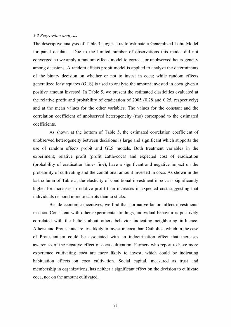
71

5.2 Regression analysis

The descriptive analysis of Table 3 suggests us to estimate a Generalized Tobit Model

for panel de data. Due to the limited number of observations this model did not

converged so we apply a random effects model to correct for unobserved heterogeneity

among decisions. A random effects probit model is applied to analyze the determinants

of the binary decision on whether or not to invest in coca; while random effects

generalized least squares (GLS) is used to analyze the amount invested in coca given a

positive amount invested. In Table 5, we present the estimated elasticities evaluated at

the relative profit and probability of eradication of 2005 (0.28 and 0.25, respectively)

and at the mean values for the other variables. The values for the constant and the

correlation coefficient of unobserved heterogeneity (rho) correspond to the estimated

coefficients.

As shown at the bottom of Table 5, the estimated correlation coefficient of

unobserved heterogeneity between decisions is large and significant which supports the

use of random effects probit and GLS models. Both treatment variables in the

experiment; relative profit (profit cattle/coca) and expected cost of eradication

(probability of eradication times fine), have a significant and negative impact on the

probability of cultivating and the conditional amount invested in coca. As shown in the

last column of Table 5, the elasticity of conditional investment in coca is significantly

higher for increases in relative profit than increases in expected cost suggesting that

individuals respond more to carrots than to sticks.

Beside economic incentives, we find that normative factors affect investments

in coca. Consistent with other experimental findings, individual behavior is positively

correlated with the beliefs about others behavior indicating neighboring influence.

Atheist and Protestants are less likely to invest in coca than Catholics, which in the case

of Protestantism could be associated with an indoctrination effect that increases

awareness of the negative effect of coca cultivation. Farmers who report to have more

experience cultivating coca are more likely to invest, which could be indicating

habituation effects on coca cultivation. Social capital, measured as trust and

membership in organizations, has neither a significant effect on the decision to cultivate

coca, nor on the amount cultivated.

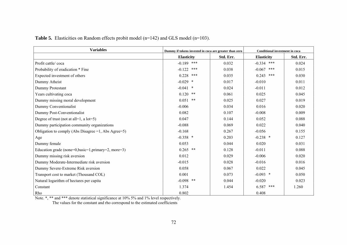
72

Table 5. Elasticities on Random effects probit model (n=142) and GLS model (n=103).

Variables Dummy if tokens invested in coca are greater than zero Conditional investment in coca

Elasticity Std. Err. Elasticity Std. Err. Profit cattle/ coca -0.189 *** 0.032 -0.334 *** 0.024 Probability of eradication * Fine -0.122 *** 0.038 -0.067 *** 0.015 Expected investment of others 0.228 *** 0.035 0.243 *** 0.030 Dummy Atheist -0.029 * 0.017 -0.010 0.011 Dummy Protestant -0.041 * 0.024 -0.011 0.012 Years cultivating coca 0.120 ** 0.061 0.025 0.045 Dummy missing moral development 0.051 ** 0.025 0.027 0.019 Dummy Conventionalist -0.006 0.034 0.016 0.020 Dummy Post-Conventionalist 0.082 0.107 -0.008 0.009 Degree of trust (not at all=1, a lot=5) 0.047 0.144 0.052 0.088 Dummy participation community organizations -0.088 0.069 0.022 0.040 Obligation to comply (Abs Disagree =1, Abs Agree=5) -0.168 0.267 -0.056 0.155 Age -0.358 * 0.203 -0.238 * 0.127 Dummy female 0.053 0.044 0.020 0.031 Education grade (none=0,basic=1,primary=2, more=3) 0.265 ** 0.128 -0.011 0.088 Dummy missing risk aversion 0.012 0.029 -0.006 0.020 Dummy Moderate-Intermediate risk aversion -0.015 0.028 -0.016 0.016 Dummy Severe-Extreme Risk aversion 0.058 0.067 0.022 0.045 Transport cost to market (Thousand COL) 0.001 0.073 -0.093 * 0.050 Natural logarithm of hectares per capita -0.098 ** 0.044 -0.020 0.023 Constant 1.374 1.454 6.587 *** 1.260 Rho 0.802 0.408 Note. *, ** and *** denote statistical significance at 10% 5% and 1% level respectively.

The values for the constant and rho correspond to the estimated coefficients

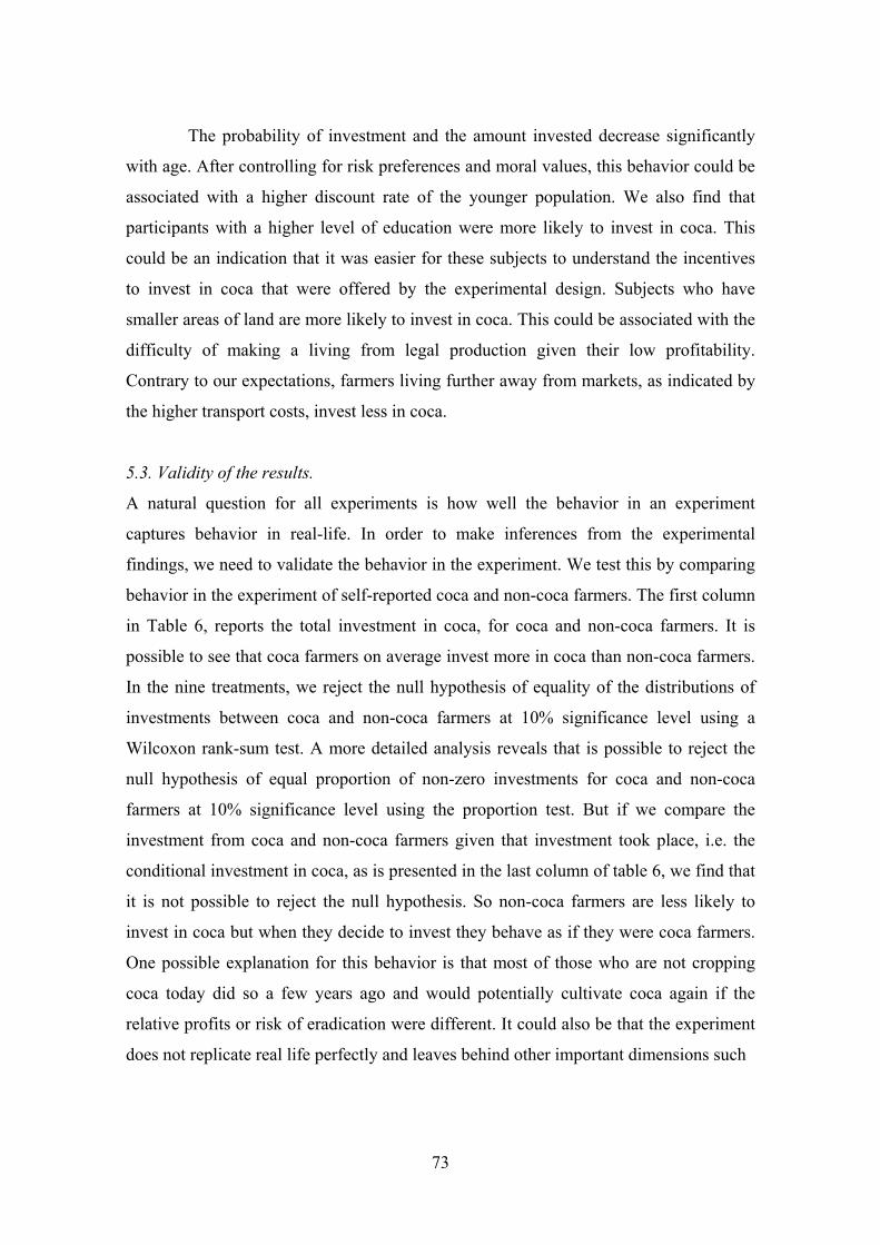
73

The probability of investment and the amount invested decrease significantly

with age. After controlling for risk preferences and moral values, this behavior could be

associated with a higher discount rate of the younger population. We also find that

participants with a higher level of education were more likely to invest in coca. This

could be an indication that it was easier for these subjects to understand the incentives

to invest in coca that were offered by the experimental design. Subjects who have

smaller areas of land are more likely to invest in coca. This could be associated with the

difficulty of making a living from legal production given their low profitability.

Contrary to our expectations, farmers living further away from markets, as indicated by

the higher transport costs, invest less in coca.

5.3. Validity of the results.

A natural question for all experiments is how well the behavior in an experiment

captures behavior in real-life. In order to make inferences from the experimental

findings, we need to validate the behavior in the experiment. We test this by comparing

behavior in the experiment of self-reported coca and non-coca farmers. The first column

in Table 6, reports the total investment in coca, for coca and non-coca farmers. It is

possible to see that coca farmers on average invest more in coca than non-coca farmers.

In the nine treatments, we reject the null hypothesis of equality of the distributions of

investments between coca and non-coca farmers at 10% significance level using a

Wilcoxon rank-sum test. A more detailed analysis reveals that is possible to reject the

null hypothesis of equal proportion of non-zero investments for coca and non-coca

farmers at 10% significance level using the proportion test. But if we compare the

investment from coca and non-coca farmers given that investment took place, i.e. the

conditional investment in coca, as is presented in the last column of table 6, we find that

it is not possible to reject the null hypothesis. So non-coca farmers are less likely to

invest in coca but when they decide to invest they behave as if they were coca farmers.

One possible explanation for this behavior is that most of those who are not cropping

coca today did so a few years ago and would potentially cultivate coca again if the

relative profits or risk of eradication were different. It could also be that the experiment

does not replicate real life perfectly and leaves behind other important dimensions such

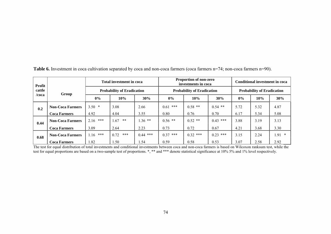
74

Table 6. Investment in coca cultivation separated by coca and non-coca farmers (coca farmers n=74; non-coca farmers n=90).

Total investment in coca Proportion of non-zero investments in coca Conditional investment in coca

Probability of Eradication Probability of Eradication Probability of Eradication Profit cattle/coca

Group 0% 10% 30% 0% 10% 30% 0% 10% 30%

Non-Coca Farmers 3.50 * 3.08 2.66 0.61 *** 0.58 ** 0.54 ** 5.72 5.32 4.87 0.2 Coca Farmers 4.92 4.04 3.55 0.80 0.76 0.70 6.17 5.34 5.08

Non-Coca Farmers 2.16 *** 1.67 ** 1.36 ** 0.56 ** 0.52 ** 0.43 *** 3.88 3.19 3.13 0.44 Coca Farmers 3.09 2.64 2.23 0.73 0.72 0.67 4.21 3.68 3.30

Non-Coca Farmers 1.16 *** 0.72 *** 0.44 *** 0.37 *** 0.32 *** 0.23 *** 3.15 2.24 1.91 * 0.68 Coca Farmers 1.82 1.50 1.54 0.59 0.58 0.53 3.07 2.58 2.92

The test for equal distribution of total investments and conditional investments between coca and non-coca farmers is based on Wilcoxon ranksum test, while the test for equal proportions are based on a two-sample test of proportions. *, ** and *** denote statistical significance at 10% 5% and 1% level respectively.

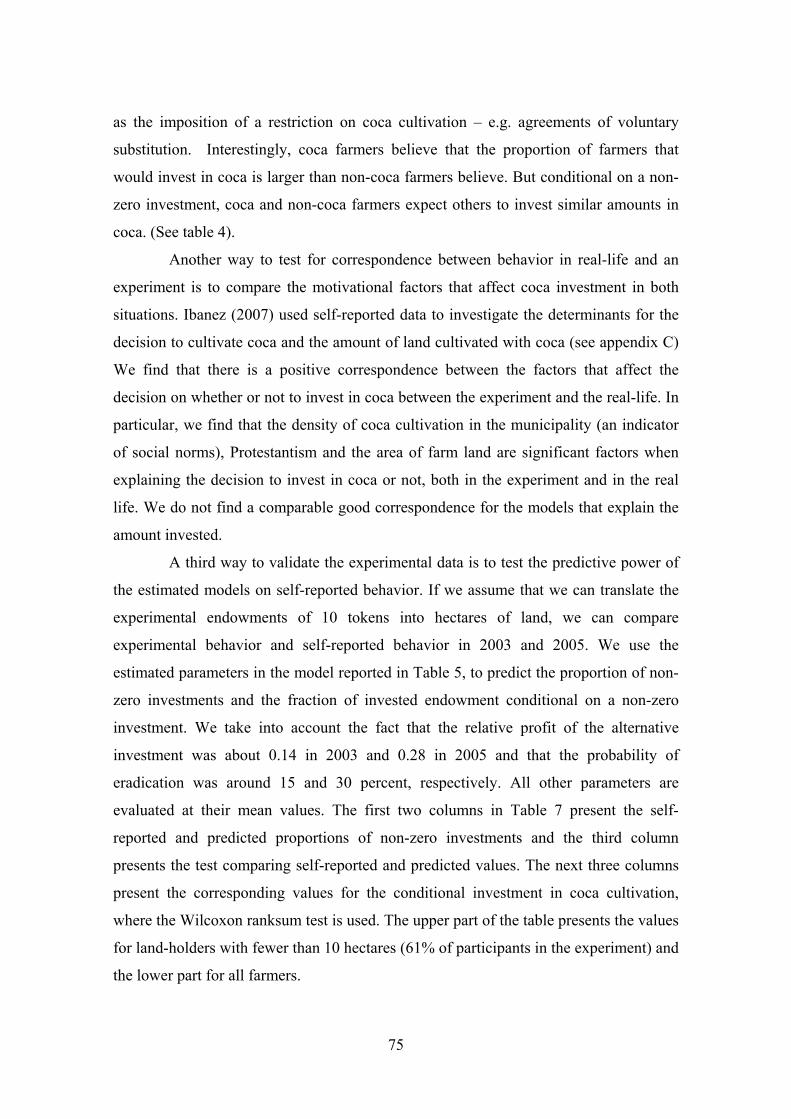
75

as the imposition of a restriction on coca cultivation – e.g. agreements of voluntary

substitution. Interestingly, coca farmers believe that the proportion of farmers that

would invest in coca is larger than non-coca farmers believe. But conditional on a non-

zero investment, coca and non-coca farmers expect others to invest similar amounts in

coca. (See table 4).

Another way to test for correspondence between behavior in real-life and an

experiment is to compare the motivational factors that affect coca investment in both

situations. Ibanez (2007) used self-reported data to investigate the determinants for the

decision to cultivate coca and the amount of land cultivated with coca (see appendix C)

We find that there is a positive correspondence between the factors that affect the

decision on whether or not to invest in coca between the experiment and the real-life. In

particular, we find that the density of coca cultivation in the municipality (an indicator

of social norms), Protestantism and the area of farm land are significant factors when

explaining the decision to invest in coca or not, both in the experiment and in the real

life. We do not find a comparable good correspondence for the models that explain the

amount invested.

A third way to validate the experimental data is to test the predictive power of

the estimated models on self-reported behavior. If we assume that we can translate the

experimental endowments of 10 tokens into hectares of land, we can compare

experimental behavior and self-reported behavior in 2003 and 2005. We use the

estimated parameters in the model reported in Table 5, to predict the proportion of non-

zero investments and the fraction of invested endowment conditional on a non-zero

investment. We take into account the fact that the relative profit of the alternative

investment was about 0.14 in 2003 and 0.28 in 2005 and that the probability of

eradication was around 15 and 30 percent, respectively. All other parameters are

evaluated at their mean values. The first two columns in Table 7 present the self-

reported and predicted proportions of non-zero investments and the third column

presents the test comparing self-reported and predicted values. The next three columns

present the corresponding values for the conditional investment in coca cultivation,

where the Wilcoxon ranksum test is used. The upper part of the table presents the values

for land-holders with fewer than 10 hectares (61% of participants in the experiment) and

the lower part for all farmers.

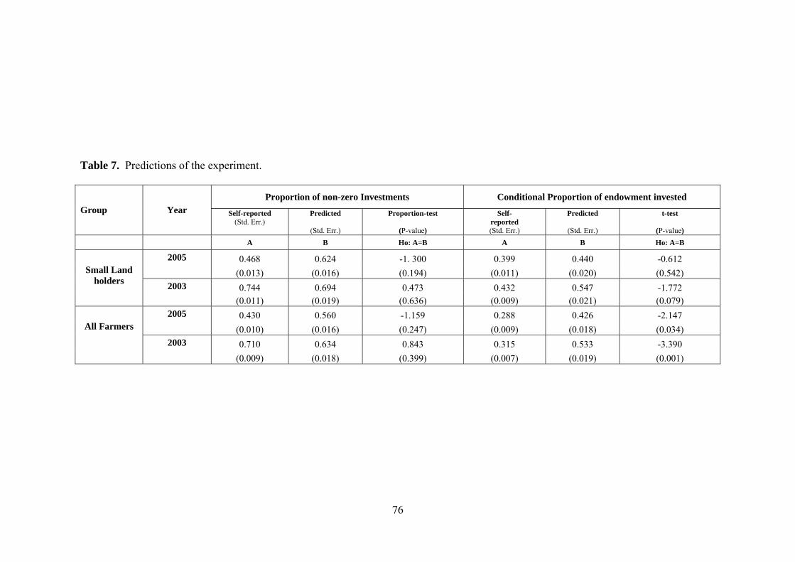
76

Table 7. Predictions of the experiment.

Proportion of non-zero Investments Conditional Proportion of endowment invested Group Year Self-reported

(Std. Err.) Predicted

(Std. Err.)

Proportion-test

(P-value)

Self- reported (Std. Err.)

Predicted

(Std. Err.)

t-test

(P-value)

A B Ho: A=B A B Ho: A=B

2005 0.468 0.624 -1. 300 0.399 0.440 -0.612 (0.013) (0.016) (0.194) (0.011) (0.020) (0.542)

2003 0.744 0.694 0.473 0.432 0.547 -1.772

Small Land holders

(0.011) (0.019) (0.636) (0.009) (0.021) (0.079) 2005 0.430 0.560 -1.159 0.288 0.426 -2.147

(0.010) (0.016) (0.247) (0.009) (0.018) (0.034) All Farmers

2003 0.710 0.634 0.843 0.315 0.533 -3.390 (0.009) (0.018) (0.399) (0.007) (0.019) (0.001)

77

The table shows that the model predicts the proportion of non-zero investments fairly

well. Using the proportion test, it is not possible to reject the null hypothesis of equality

in the proportion of non-zero investments between self-reported and predicted values at

10% significance level. The prediction ability of the model is lower for the conditional

investment. Except for small farmers in 2005, we reject the null hypothesis of equality

on self-reported and predicted conditional proportions of the endowments at 10%

significance level using the t-test. It should be noted that in the experiment, we used a

standardized unit of 10. In real-life however, the areas of land differ and although a

farmer can own say 100 hectares, he/she would rarely maintain more than 3 hectares

with coca. This is probably a strategy to reduce the risk of having the crops destroyed.

According to discussions with farmers, labor requirements seem to limit the amount of

land that is cultivated with coca. Our results suggest that the experimental setting that

we used captures some aspects of self-reported behavior. This therefore allows us to

use the experiment to analyze policy implications on policy levels, especially for

households with under 10 hectares of land.

5.4. Partial equilibrium analysis of stick and carrot analysis

Based on the estimated model, we conduct a partial equilibrium analysis of the stick and

carrot policy on the proportion of non-zero investments and the proportion of invested

endowment. Figures 1, 2 and 3 present the predicted proportion of non-zero

investments, the conditional investment and the total investment in coca at different

levels of relative profit of cattle and probability of eradication. We focus only on small-

land holders. Forecasting the results of the experiment across the range of possible

relative prices and probabilities of eradication used in the experimental setting, it is

interesting to note that the model predicts that not all farmers will cultivate coca and

that not all land will be cultivated even when the relative profit and the probability of

eradication are low. According to the predictions of the model, about 37% of the total

endowment would be invested in coca when the economic incentives are extremely

favorable to do so. The model also predicts that if the profit from cattle is high (68%)

and the probability of eradication is high (30%) the proportion of the total endowment

invested in coca will be lower than 10%. In addition, the model predicts that in the

absence of alternatives - when the relative profit of cattle is too low - eradication will

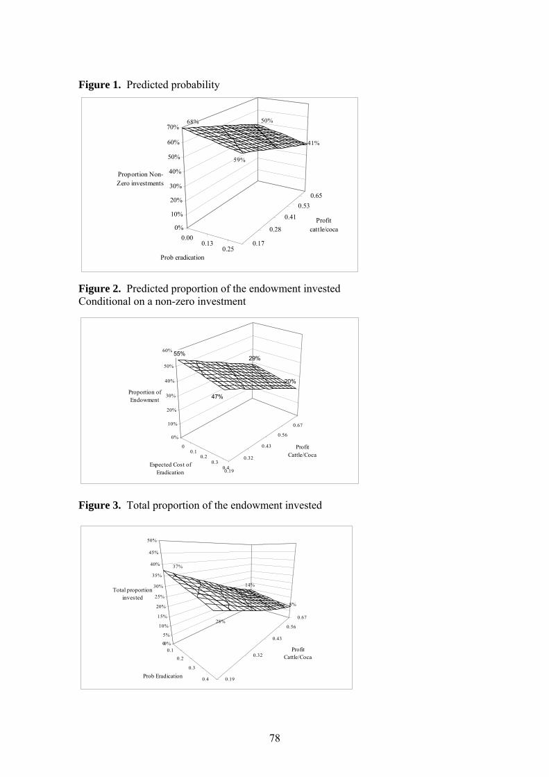
78

Figure 1. Predicted probability Figure 2. Predicted proportion of the endowment invested Conditional on a non-zero investment Figure 3. Total proportion of the endowment invested

00.1

0.2

0.3

0.4 0.19

0.32

0.43

0.56

0.67

0%

5%

10%

15%

20%

25%

30%

35%

40%

45%

50%

Prob Eradication

ProfitCattle/Coca

Total proportion invested

37%

28%

14%

8%

0.000.13

0.250.17

0.28

0.41

0.530.65

0%

10%

20%

30%

40%

50%

60%

70%

Proportion Non-Zero investments

Prob eradication

Profitcattle/coca

68%

59%

41%

50%

00.1

0.20.3

0.40.19

0.32

0.43

0.56

0.67

0%

10%

20%

30%

40%

50%

60%

Proportion of Endowment

Expected Cost of Eradication

Profit Cattle/Coca

55%

47%

29%

20%

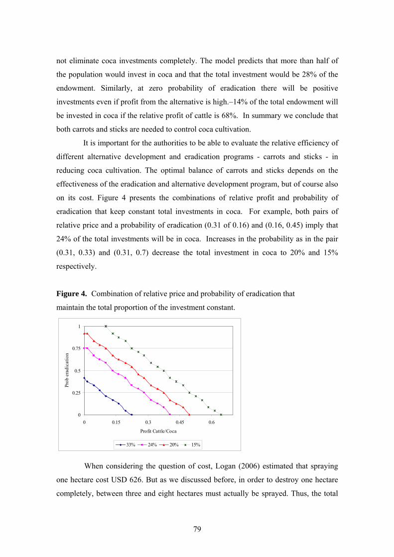
79

not eliminate coca investments completely. The model predicts that more than half of

the population would invest in coca and that the total investment would be 28% of the

endowment. Similarly, at zero probability of eradication there will be positive

investments even if profit from the alternative is high.–14% of the total endowment will

be invested in coca if the relative profit of cattle is 68%. In summary we conclude that

both carrots and sticks are needed to control coca cultivation.

It is important for the authorities to be able to evaluate the relative efficiency of

different alternative development and eradication programs - carrots and sticks - in

reducing coca cultivation. The optimal balance of carrots and sticks depends on the

effectiveness of the eradication and alternative development program, but of course also

on its cost. Figure 4 presents the combinations of relative profit and probability of

eradication that keep constant total investments in coca. For example, both pairs of

relative price and a probability of eradication (0.31 of 0.16) and (0.16, 0.45) imply that

24% of the total investments will be in coca. Increases in the probability as in the pair

(0.31, 0.33) and (0.31, 0.7) decrease the total investment in coca to 20% and 15%

respectively.

Figure 4. Combination of relative price and probability of eradication that

maintain the total proportion of the investment constant.

0

0.25

0.5

0.75

1

0 0.15 0.3 0.45 0.6

Profit Cattle/Coca

Prob

era

dica

tion

33% 24% 20% 15%

When considering the question of cost, Logan (2006) estimated that spraying

one hectare cost USD 626. But as we discussed before, in order to destroy one hectare

completely, between three and eight hectares must actually be sprayed. Thus, the total

80

cost of destroying one hectare is between 1,878 USD and 5,008 USD. In 2003, the

government established a monetary subsidy by which households who agreed to keep

their land free of coca received 1,524 USD yearly during three years compared with an

average profit of 1,402 USD per hectare year of coca (Ibanez, 2007). On average,

households that participated in the program in Putumayo agreed to keep 10 hectares free

of coca, so the average cost of the subsidy per hectare year is 152 USD. In other words

destroying one hectare by spraying is between 12 to 33 times more expensive than

offering a monetary subsidy. However, the total cost of the eradication policy depends

on the total number of hectares of coca that need to be sprayed and the total number of

potential beneficiaries from the subsidy. If the number of hectares declared by potential

beneficiaries of the subsidy is higher than the number of hectares that need to be

sprayed, then spraying would be preferable to the alternative development.

6. Conclusions

Existing data on the amount of investment in coca under different regimes of carrot and

stick policies in Colombia is limited to data at the municipal level based on revealed

preferences. By using a framed field experiment, we mimic the decision that Colombian

farmers in the department of Putumayo are faced with. Thus, our experimental approach

allows us to investigate how farmers react to a wide range of different combinations of

stick and carrot policies. In subsequent analyses, we compared the behavior in the

experiment and in real-life, and the overall comparison suggests that experimental

behavior is consistent with real-life coca cultivation. Our main results support earlier

findings, based on municipal data, that changes in relative profit have more impact on

reducing coca cultivation than changes in the probability of eradication do.

In terms of policy recommendations, our results suggest that both eradication

and alternative development are needed to reduce coca cultivation. Although the cost of

destroying one hectare is higher than the cost of the subsidy offered by the authorities, it

may still be cost-effective to use eradication when the number of hectares to be

subsidized is substantially higher than the number of hectares of coca to be eradicated.

The current form of voluntary agreement to substitute coca with alternative

development is a direct monetary pay-off. However, the longer-term strategy is to

increase the relative profit more permanently by, for example, improving the

81

infrastructure or undertaking policies that tackle the agricultural crisis in Colombia.

Related to this is the issue of the effect of eradication on the income of farmers. If the

two policies are expected to result in the same amount of coca cultivation, then the

policy that has a higher level of eradication will cause a greater number of farmers to be

below the poverty line because farmers loose their income if their coca fields are

eradicated. Since many of the farmers are living close to or under the poverty line, it

may explain why they respond to changes in relative profit more than they do to

changes in eradication levels. Thus, a mix of policies resulting in the same amount of

coca cultivated may have very different impacts on welfare, especially on those farmers

who are below the poverty line. Our results suggests that a more systematic social

welfare analysis of stick and carrot policies is needed in general, but also that the use of

alternative development programs to increase the relative profits of non-coca activities

seems to be a promising way of reducing coca cultivation.

82

7. References Akerlof, George A. 1997. “Social distance and Social Decisions”. Econometrica. 65 (September): 1005-

1028. Alm, James, Betty R. Jackson, Michael McKee. 1992a. “Estimating the determinants of tax payer

compliance with experimental data”. National Tax Journal. 45. (March): 107-114. Alm, James, Gary H. McClelland and William D. Schulze. 1992b. “Why do people pay taxes?” Journal

of Public Economics. 48 (June): 21-38. Anderson, Lisa R. and Sarah Stafford. 2003. “Punishment in a Regulatory setting: experimental evidence

from VCM.” Journal of Regulatory Economics. 24 (July): 91-110. Barr, Abigail and Pieter Serneels. 2004. “Wages and reciprocity in the workplace”. Mimeo, Oxford

University, Centre for the Study of African Economies. Binswanger, Hans P. 1980. “Attitude towards risk: experimental measurement in rural India” American

Journal of Economics. 62(August): 395-407. Calvo-Armengol, Antoni and Yves Zenou. 2004. “Social networks and crime decisions: The role of social

structure in facilitating delinquent behavior.” International Economic Review. 45 (August): 939-58. Cardenas, Juan Camilo, John Stranlund and Cleve Willis. 2000. “Local Environmental Control and

Institutional Crowding-Out.” World Development. 28 (October): 1719-33. Cardenas, Juan Camilo and Elionor Ostrom. 2004. “What do people bring into the game? Experiments in

the field about cooperation in the commons.” Agricultural Systems. 82. (December): 307-26. Cardenas, Juan Camilo. 2004. “Norms from Outside and from Inside: An Experimental Analysis on the

Governance of Local Ecosystems.” Forest Policy and Economics. 6 (June): 229-41. Cardenas, Juan Camilo. 2005. “Groups, Commons and Regulations: Experiments with Villagers and

Students in Colombia”, In Agarwal, Bina and Alessandro Vercelli Ed. 2005. “Psychology, Rationality and Economic Behavior: Challenging Standard Assumptions.”

Carpenter, Jeffrey P. and E. Seki. 2004. “Do Social Preferences Increase Productivity? Field Experimental Evidence from Fishermen in Toyama Bay”. IZA DP No. 1697. (July)

Carvajal, Maria Paula. 2002. “Factores explicativos de la presencia de cultivos ilícitos en los municipios de Colombia” Dissertation. CEDE- Universidad de los Andes. Bogotá, Colombia.

Colby, Anne and Laurent Kohlberg. 1987. “The Measurement of Moral Judgment, Vol. 1: Theoretical Foundations and Research Validation.” Cambridge: Cambridge University Press.

Díaz, Ana-Maria and Sánchez. 2004. “Geography of Illicit Crops and Armed conflict in Colombia” Universidad de los Andes. Document CEDE 2004-18. (March).

DNE. 2005. “Observatorio de Drogas de Colombia: Acciones y Resultados” Dirección Nacional de Estupefacients. Subdirección estratégica y de investigaciones. Bogota, Colombia.

DNE. 2006. “Observatorio de Drogas de Colombia 1999-2005” Direccion Nacional de Estupefacients. Subdirección estratégica y de investigaciones. Bogota, Colombia.

Eckel, Catherine and Philip J. Grossman. 1996. “Altruism in anonymous dictator games.” Games and Economic Behavior, 16 (October): 161-81.

Eisenhauer, Joseph. 2004. “Economic Models of Sin and Remorse: Some Simple Analytics.” Review of Social Economy, 62 (June): 201-19.

Falk, Armin and Urs Fischbacher. 2002. “Crime in the lab-detecting social interaction” European Economic review, 46 (May): 859-69.

Falk, Armin, Urs Fischbacher and Simon Gächter. 2004. “Living in two neighbourhoods: Social interactions in the lab.” IZA - Discussion paper No. 1381.

Fehr, Ernst and Simon Gachter. 2000. “Cooperation and Punishment in Public good Experiments” American Economic Review. 90 (September): 980-94.

Fehr, Ernst, Simon Gächter and Georg Kirchsteiger. 1997. “Reciprocity as a contract enforcement device” Econometrica, 65 (July): 833-60.

Feld, Lars and Jean-Robert Tyran. 2002. “Tax evasion and Voting: and experimental analysis” Kyklos, 55 (May): 197-222.

Fischbacher, Urs and Simon Gächter. 2006. “Heterogeneous social preferences and the dynamics of free riding in public goods.” Discussion Paper 2006-01. University of Nottingham (January).

Fischbacher, Urs, Simon Gächter and Ernst Fehr. 2001. “Are people conditional cooperative? Evidence from a public goods experiment”. Economics Letters. 71 (June): 397-404.

Forero, Jaime, Juan Andres Galarza, Luz Elba Torres, Jose Luis Forero. 2002. “La economía campesina Colombiana 1990-2001” Cuadernos tierra y Justicia No. 2. Pontificia Universidad Javeriana.

83

Fortin, Bernard, Guy Lacroix, Marie-Claire Villeval. 2004. “Tax evasion and social interactions: an experimental approach” IZA - Discussion paper No. 1359. Institute for the study of labor. (October)

Gächter, Simon and Elke Renner. 2006. The effects of (incentivized) belief elicitation in public good experiments. Nottingham University. Discussion paper 2006-16. (September).

Galbiati, Roberto and Pietro Vertova. 2005. “Law and behavior in social dilemmas: Testing the effect of obligations on cooperation” Tilburg University. CentER Discussion paper No. 2005-56.

Garoupa, Nuno. 2003. “Crime and Social Norms.” Portuguese Economic Journal. 2 (December): 131-44. Glaeser, Edward L. Bruce Sacerdote, and Jose Scheinkman. 1996. “Crime and Social Interactions.” The

Quarterly Journal of Economics, 111 (May): 508–48. Harrison, Glenn W. and John A. List. 2004. “Field experiments” Journal of Economic Literature, 42

(December): 1009-55. Hatcher, Aaron, Shabbar Jaffry, Olivier Thébaud, and Elizabeth Bennett. 2000. “Normative and Social

Influences Affecting Compliance with Fishery Regulations.” Land Economics. 76 (August): 448-61.

Ibanez, Marcela. 2007. “Who crops coca and why?” Mimeo. Göteborg University. Karlan, Dean. 2006. “Using Experimental Economics to Measure Social Capital and Predict Financial

Decisions.” American Economic Review, 95(5), 1688-99. Kuperan K. and Jon Sutinen. 1998. “Blue water crime: Deterrence, Legitimacy and compliance in

fisheries”. Law and Society Review. 32: 309-38. Levitt, Steven D. and John A. List. 2007. “What do Laboratory experiments tell us about the real world”

Forthcoming Journal of Economic Perspectives. Lind, George Hans A. Hartmann and Roland Wakenhut (Eds). 1985. “Moral development and the social

environment studies in the philosophy and psychology of moral judgment and education”. Loewenstein, George and David Schkade. 1999. “Wouldn’t it be nice? Predicting future feelings.” In:

Kahneman, Daniel., Ed Diener, Norbert Schwartz (Eds.). 1999. “Well-Being: The Foundations of Hedonic Psychology.” Russell Sage, New York.

Logan, Sam. 2006. “Hydras, Ballons wasted Money in los Andes.” ISN Security Watch in Buenos Aires. Moreno Sanchez, Rocio, David S. Kraybill and Stanley R. Thompson. 2003. “An econometric analysis of

coca eradication policy in Colombia.” World Development. 31 (February): 375-383. Moya, Andres. 2005. “Impacto de la erradicacion forzosa y el desarrollo alternativo sobre los cultivos de

coca.” Dissertation paper. Universidad de los Andes. Bogotá, Colombia. Murphy, James J. and Juan Camilo Cardenas. 2004. “An Experiment on Enforcement Strategies for

Managing a Local Environmental Resource.”. Journal of Economic Education. 35 (Winter): 47-61. Nadler, Janice. 2005. “Flouting the law: does perceived injustice provoke general non-compliance?”

Texas Law Review. 83 (April): 1399-1441. Offerman, Theo, Joep Sonnemans and Arthur Schram. 1996. “Value Orientations, Expectations and

Voluntary Contributions in Public Goods.” Economic Journal. 106 (July): 817-45. Ostrom, Eleonor, James Walker and Roy Gardner. 1992. “Covenants with and without a sword: Self-

governance is possible.” The American Political Science Review. (June): 404-417. Perez, Ricardo, Andres Vergara and Yilberto LaHuerta. 2002. “Approximación metodológica y

cuantitativa de los costos económicos generados por el problema de las drogas ilícitas en Colombia (1995-2000).” Archivos de Economía. DNP. Colombia.

Potters, Jan and Frans van Winden. 2000. “Professional and students in a lobbying experiment. Professional rules of conduct and subject surrogacy.” Journal of Behavioral Economics and Organization, 43 (December): 499-522.

Sefton, Martin, Robert Shupp and James Walter. 2000. “The effect of rewards and Sanctions in the provision of Public goods” Indiana University. Bloomington, IN

Sonnemans, Joep, Arthur Schram and Theo Offerman. 2001. “Is the quadratic scoring rule really incentive compatible?” Mimeo. University of Amsterdam.

Sugden, Robert. 1984. “Reciprocity: The supply of public goods through voluntary contributions.” Economic Journal. 94 (December): 772-787.

Sutinen, Jon. G. and K. Kuperan. 1999. "A Socio-Economic Theory of Regulatory Compliance," International Journal of Social Economics. 26 (No 1): 174-93.

Sutter, Mattias, Stefan Haigner and Martin Kocher. 2006. “Choosing the stick of the carrot? Endogenous institutional choice in social dilemma situations” University of Innsbruck. CEPR Discussion Paper 5497. (February).

Tabares, Elizabeth and Ramón Rosales. 2004. “Politicas de control de oferta de coca: La zanahoria y el garrote.” Universidad de los Andes. Document CEDE 2005-10 (January).

84

Trivedi V. Umashanker, Mohamend Shehata and Bernadette Lynn. 2003. “Impact of personal and situational factors on taxpayer compliance: an experimental analysis.” Journal of Business Ethics. 47 (October): 175-97.

Trivedi, Viswanath Umashanker, U., Mohamed Shehata and Stuart Mestelman. 2005. “Attitudes incentives and tax compliance.” Canadian Tax Journal, 53 (1): 29-61.

Tyler, Tom R. 1990. “Why People Obey the Law”. New Haven, CT: Yale Univ. Press. Tyran Jean-Robert and Lars Feld. 2002. “Why people obey the law experimental evidence from the

provision of public goods.” CESifo Working Paper No. 651 (January). UN. 1961. “Single Convention against Narcotic Drugs”. United Nations.

85

Appendix A

Instructions

Good afternoon and welcome to this workshop. Before we start we would like to thank you for your

assistance. In this workshop you will have the opportunity to earn some money. The amount of money

that you will earn depends on your own decisions as well as the decisions of others. This workshop is

organized by Universidad de los Andes en Bogota. The results of this study will be used for academic

purposes. Throughout the exercise we will not ask for your name, where you live or pose any other

question that allows us to identify you or your family. The answers will not be presented individually.

How long is the exercise?

This workshop will take approximately two hours. You will be asked to make 9 different decisions. At a

first glance they may seem to be similar, but they do, in fact, differ. Therefore it is important to think

about each decision carefully.

What kinds of decision will you be asked to make?

We will randomly form groups of five people. You will not know to which group you belong either

during or after the workshop. You will remain in the same group for all 9 decisions.

For each decision you will receive 10 tokens. These tokens are equivalent in real life to the land, the

available hours of work and the money you have available to cultivate your crops. Your first task is to

decide how many tokens you would like to invest in two agricultural products. Your second task is to

guess how much the other four people in your group will invest in coca. Please consider what you would

do in real life.

What are the characteristics of the investments?

The two agricultural products are coca and cattle raising. They have different returns. For each token you

invest in coca you get 1250 pesos. For each token that you invest in cattle raising you will get 250 pesos.

Cropping coca generates negative effects for the community such as increased levels of violence,

environmental damage, increases in prices in the region, etc. Therefore for each token that you invest in

coca, the incomes of you as well as the other members in your group will be reduced by 212.5 pesos.

Similarly, for each token that others invest in coca, the incomes of you as well as the other members of

your group, will be reduced by 212.5 pesos.

86

How is your payment calculated?

At the beginning of the workshop you will receive 15.000 pesos but depending upon your decisions and

the decision of others in your group, you can earn more or less than that amount. Your payment can be

lower than 15.000 pesos but even in the worst case you will earn a certain amount. In the workshop you

have to take9 decisions but only one of these will be paid. Which decision is paid is selected randomly, so

consider each decision carefully.

Let us look at an example.

As we explained before, for each token that you invest in cattle raising you obtain 250 pesos and for each

token that you invest in coca you obtain 1250 pesos. {Write numbers on the blackboard}. Let us say that

you, for example, have invested 7 tokens in coca and 3 tokens in cattle raising, while other people in your

group have invested 27 tokens in coca. In this case, your earnings from coca are 7 tokens times 1.250

which is 8.550 pesos. The earnings from investing in cattle raising are 3 tokens times 250 pesos or 750

pesos. Due to the negative effect from coca of violence, environmental damage and increased prices,

there is a reduction in earnings from coca investments. You invested 7 and the others 27 and in total this

is 34 tokens. The reduction in tokens for investing in coca is thus 34 tokens times 212.5 pesos that is

7,225 pesos.

Investment in coca 7 x 1250 8.750

Investment in cattle raising 3 x 250 750

Reduction -34 x 212,5 -7.225

In Pesos 2 275

To make this calculation easier, we have prepared a payment table that summarizes your earnings in

pesos {show a poster with an enlarged pay-off table}. This table is called “Pay-off table”. Note that the

top of the table indicates the return from coca and cattle raising. In the green table, for each token

invested in cattle raising you receive 250 pesos. The columns indicate the number of tokens you invested

in coca and cattle raising. The rows indicate the number of tokens that the others invested in coca and

cattle raising. Continuing with our example, if you invested 7 tokens in coca {move along to column 7

using one hand} and 3 tokens in cattle raising and if the others invested 27 in coca {move down to row 27

with left hand side} and 13 tokens in cattle raising then your earning in pesos would be 2 275 {find

intersection in the table}. Remember, what you do not invest in coca is automatically invested in cattle

raising. In other words, the sum of your investment in coca and cattle raising is 10 tokens.

Let us look at another example. If you invest 4 tokens in coca and 6 tokens in cattle raising and the others

invest 17 tokens in coca and 23 in cattle raising. In the table, four tokens invested by you {move with the

87

right hand side to column 4} and 17 tokens invested by others {move with left hand side to row 17}

imply a payment of 2.038 pesos. Do you have any question so far?

Correct guess

You can increase your earnings by correctly guessing how much the others have invested in coca. The

closer your guess is to the investment of others the higher your reward will be. Do you think that the

others will do the same as you did? Do you think they will invest more in coca? Do you think they will

invest less?

Procedures

We start by sitting down in the room. Once you are seated in the assigned place you will receive your

decision sheets and payment tables. Please write your birth date (year/month/day) and the last three digits

of you I.D. number. This is your identification number. Once you have handed in your decision sheet we

will put all the identification numbers in a bag and draw them to form groups of five people. You will not

know who belongs to your group but in the nine decisions you will remain in the same group.

The decision sheet contains 9 choices/dilemmas/questions[?]. The first column of the decision sheet

explains the particular characteristics of the case under consideration, in the second column you should

write how many tokens you would like invest in coca. What you do not invest in coca is automatically

invested in cattle raising. In the last column you should write how many tokens you expect the others will

invest in coca. The others can, in total, invest anything between 0 and 40 tokens.

There are three payment tables. The green table indicates the payments when each token invested in cattle

raising yields 250 pesos. The red table indicates the payments when each token invested in cattle raising

yields 550 pesos and the blue table indicates the payments when each token invested in cattle raising

yields 850 pesos. Once you have completed the first three decisions, we will explain the next 6 decisions

and the procedure to be applied in the second half of the workshop. After the nine decisions have been

completed we will select a letter from a bag to decide which decision is to be paid. The payment will be

made in a coupon that can be exchanged in the super market.

Do you have any question so far?

Once we have started you should not talk to anyone in the room. Those who talk will be excluded from

the workshop and the payments. If you have any question please raise your hand and one of us will come

and answer your query.

88

{Distribute register sheet and form groups} We want to ask you to come to the front so that we

canallocate places for you to sit in the room. {Allocate seats and hand in practice questions}

Practice questions

Before we begin with the investment decisions, you will make some hypothetical decisions. The idea is to

make sure that we have managed to explain the experiment clearly to you. These decisions will not affect

your payment.

1. If you obtain 1250 pesos for every token invested in coca and 250 pesos for each token invested

in cattle raising:.

How many tokens do you want to invest in coca? _________ tokens

How many tokens do you think that the others will invest in coca? _________ tokens

What would your payment be? _________ pesos

Once you have finished making your decisions, we will come and collect the first page of the form. Then

we will determine whether eradication will happen or not by drawing balls from a bag. We will make one

draw for each decision and the outcome of whether or not crop is being controlled by eradication will be

the same for all of you. To ensure confidentiality, you will receive your payment in an envelope with your

ID number when you leave.

Now we will explain the following six decisions.

Regulation and Control

Investment in coca is illegal and thus there is a risk that your investment will be detected. This will not

necessarily be the case. To determine whether your crop is eradicated, we will draw a ball from a bag. If a

green ball is selected then it is not. If a red ball is selected then it is eradicated. The proportion of red and

green balls changes from case to case. In three cases the bag contains one red ball and 9 green balls and in

the other three cases the bag contains 3 red balls and 7 green balls. If your crop is eradicated, you will

lose 1500 pesos for each token invested in coca. But as in real life, eradication does not always occur.

Example

Let us consider the case where there are 9 green balls and 1 red ball . We put 9 green balls and one red

ball in the bag. {Make demonstration}. If we continue with our first example in which you invested 7

tokens in coca and the others invested 27 tokens, and your income was 2 275 pesos, if there eradication

took place your income would be reduced by 10 500 pesos. Why 10 500 pesos? You have invested 7

tokens and each token results in a cost of 1500 pesos so the total cost is 10 500 pesos. When there was no

eradication your income was 2 275 but with eradication you must subtract10 500 which makes -8 225

89

pesos. If this decision is selected for payment, you would receive 4 500 pesos, that is 15 000 pesos minus

8 225pesos.

For the next six decisions we will follow the same procedure that we used before. First we will have some

practice questions to make sure that our explanation is clear. Then you can complete the next six

decisions. When you make your decisions you will have time to look at them again and make corrections.

If you want to change a decision please mark a line over the decision so it is still possible to see the initial

value and write down the new value. When you have finished, we will collect the decision sheets, select

which alternative will be paid and determine whether eradication will take place or not by taking a ball

from the bag. We will take one ball and the result will be applied to everyone in the group.

Practice questions

2. If you obtain 1250 pesos for every token invested in coca and 250 pesos for each token that you

invest in cattle raising and if a red ball is selected meaning that eradication will take place. and

you will need to pay 1500 pesos for each token invested in coca and if there are 9 green balls and

one red ball.:.

How many tokens do you want to invest in coca? _________ tokens

How many tokens do you think that the others will invest in coca? _________ tokens

What would your payment be if there is no eradication? _________ pesos

What would your payment be if there is eradication ? _________ pesos

90

Decision Sheet You have 10 tokens that you can invest in coca or in cattle raising. Your task is to decide how many tokens you would like to invest in coca and how much you expect others in your group will invest in coca. PLEASE USE THE TABLE TO STUDY THE OUTCOME OF DIFFERENT DECISIONS. Please consider what you would do in real life.

Decision Case Your

investment in Coca

Your investment in Cattle raising

Expected investment of others in

coca

A. 1 token in coca gives 1250 pesos 1 token in cattle raising gives 250 pesos. 1 token in coca cost 212,5 to each person in the group.

B. 1 token in coca gives 1250 pesos 1 token in cattle raising gives 550 pesos. 1 token in coca cost 212,5 to each person in the group.

C. 1 token in coca gives 1250 pesos 1 token in cattle raising gives 850 pesos. 1 token in coca cost 212,5 to each person in the group.

D. 1 token in coca gives 1250 pesos 1 token in cattle raising gives 250 pesos. 1 token in coca cost 212,5 to each person in the group.

If a red ball is selected there is control. If this happens you have to pay 1500 pesos for each token in coca. There is one red ball and 9 green balls.

E. 1 token in coca gives 1250 pesos 1 token in cattle raising gives 550 pesos. 1 token in coca cost 212,5 to each person in the group.

If a red ball is selected there is control. If this happens you have to pay 1500 pesos for each token in coca. There is one red ball and 9 green balls.

F. 1 token in coca gives 1250 pesos 1 token in cattle raising gives 850 pesos. 1 token in coca cost 212,5 to each person in the group.

If a red ball is selected there is control. If this happens you have to pay 1500 pesos for each token in coca. There is one red ball and 9 green balls.

G. 1 token in coca gives 1250 pesos 1 token in cattle raising gives 250 pesos. 1 token in coca cost 212,5 to each person in the group.

If a red ball is selected there is control. If this happens you have to pay 1500 pesos for each token in coca. There are 3 red balls and 7 green balls.

H. 1 token in coca gives 1250 pesos 1 token in cattle raising gives 550 pesos. 1 token in coca cost 212,5 to each person in the group.

If a red ball is selected there is control. If this happens you have to pay 1500 pesos for each token in coca. There are 3 red balls and 7 green balls.

I. 1 token in coca gives 1250 pesos 1 token in cattle raising gives 850 pesos. 1 token in coca cost 212,5 to each person in the group.

If a red ball is selected there is control. If this happens you have to pay 1500 pesos for each token in coca. There are 3 red balls and 7 green balls.

91

Appendix B

Each token invested in coca gives 1250 Pesos Each token invested in cattle raising gives 250 Pesos

Pay-off Table when there is no eradication Your investment in Coca 0 1 2 3 4 5 6 7 8 9 10

0 2500 3300 4100 4900 5700 6400 7200 8000 8800 9600 10400 1 2300 3100 3900 4700 5400 6200 7000 7800 8600 9400 10200 2 2100 2900 3700 4400 5200 6000 6800 7600 8400 9200 10000 3 1900 2700 3400 4200 5000 5800 6600 7400 8200 9000 9700 4 1700 2400 3200 4000 4800 5600 6400 7200 8000 8700 9500 5 1400 2200 3000 3800 4600 5400 6200 7000 7700 8500 9300 6 1200 2000 2800 3600 4400 5200 6000 6700 7500 8300 9100 7 1000 1800 2600 3400 4200 5000 5700 6500 7300 8100 8900 8 800 1600 2400 3200 4000 4700 5500 6300 7100 7900 8700 9 600 1400 2200 3000 3700 4500 5300 6100 6900 7700 8500

10 400 1200 2000 2700 3500 4300 5100 5900 6700 7500 8300 11 200 1000 1700 2500 3300 4100 4900 5700 6500 7300 8000 12 -100 700 1500 2300 3100 3900 4700 5500 6300 7000 7800 13 -300 500 1300 2100 2900 3700 4500 5300 6000 6800 7600 14 -500 300 1100 1900 2700 3500 4300 5000 5800 6600 7400 15 -700 100 900 1700 2500 3300 4000 4800 5600 6400 7200 16 -900 -100 700 1500 2300 3000 3800 4600 5400 6200 7000 17 -1100 -300 500 1300 2000 2800 3600 4400 5200 6000 6800 18 -1300 -500 300 1000 1800 2600 3400 4200 5000 5800 6600 19 -1500 -800 0 800 1600 2400 3200 4000 4800 5600 6300 20 -1800 -1000 -200 600 1400 2200 3000 3800 4600 5300 6100 21 -2000 -1200 -400 400 1200 2000 2800 3600 4300 5100 5900 22 -2200 -1400 -600 200 1000 1800 2600 3300 4100 4900 5700 23 -2400 -1600 -800 0 800 1600 2300 3100 3900 4700 5500 24 -2600 -1800 -1000 -200 500 1300 2100 2900 3700 4500 5300 25 -2800 -2000 -1200 -500 300 1100 1900 2700 3500 4300 5100 26 -3000 -2200 -1500 -700 100 900 1700 2500 3300 4100 4900 27 -3200 -2500 -1700 -900 -100 700 1500 2300 3100 3900 4600 28 -3500 -2700 -1900 -1100 -300 500 1300 2100 2900 3600 4400 29 -3700 -2900 -2100 -1300 -500 300 1100 1900 2600 3400 4200 30 -3900 -3100 -2300 -1500 -700 100 900 1600 2400 3200 4000 31 -4100 -3300 -2500 -1700 -900 -200 600 1400 2200 3000 3800 32 -4300 -3500 -2700 -1900 -1200 -400 400 1200 2000 2800 3600 33 -4500 -3700 -2900 -2200 -1400 -600 200 1000 1800 2600 3400 34 -4700 -3900 -3200 -2400 -1600 -800 0 800 1600 2400 3200 35 -4900 -4200 -3400 -2600 -1800 -1000 -200 600 1400 2200 2900 36 -5200 -4400 -3600 -2800 -2000 -1200 -400 400 1200 1900 2700 37 -5400 -4600 -3800 -3000 -2200 -1400 -600 100 900 1700 2500 38 -5600 -4800 -4000 -3200 -2400 -1600 -900 -100 700 1500 2300 39 -5800 -5000 -4200 -3400 -2600 -1900 -1100 -300 500 1300 2100

Inve

stm

ent o

f oth

ers i

n co

ca

40 -6000 -5200 -4400 -3600 -2900 -2100 -1300 -500 300 1100 1900

92

Appendix C.

Coca cultivation decisions with self-reported data.

Decision to cultivate coca

Proportion of land cultivated with coca

n=329 n=214

Elasticity Coef. Std. Err.

Variables

Log profit coca -0.349 0.008 0.008 Log profit alternative -0.054 -0.004 0.011 Index of Market conditions -0.005 -0.010 0.027 Sprayed ha/Total ha with coca in municipality -0.066 *** 0.001 0.014 Dummy Atheists -0.003 0.057 0.038 Dummy Protestant -0.029 *** 0.082 0.224 Years cultivating coca 0.048 -0.003 0.006 Moral development (Missing=0; Pre-Conv=1; Conv=2; Post-Conv=3) -0.052 0.020 0.018 Degree of trust (not at all=1, a lot=5) 0.040 0.010 0.009 Dummy participation in communitary organizations -0.024 -0.006 0.027 Ha with coca/Municipal Area 0.264 *** 0.001 0.003 Obligation to comply (Compl disagree=1, Compl. Agree=5) -0.455 *** 0.024 0.044 Age -0.087 -0.008 0.007 Squared Age 0.065 0.000 0.000 Female -0.011 -0.111 *** 0.026 Education (None=0,Basic=1, Primary=2, More=3 0.047 -0.008 0.083 Squared Education Grade 0.038 0.009 0.014 Coefficient of relative risk aversion. 0.002 0.003 0.003 Cost of transport (Thousand COL) 0.004 0.004 0.005 Log Land per capita -0.089 *** -0.152 ** 0.067 Dummy missed stage moral development 0.034 ** 0.064 0.134 Dummy missed risk aversion -0.004 0.287 0.541 Dummy Participation Substitution Program - -0.069 *** -0.063 0.166 Probability of non-zero investment -0.063 *, ** and *** denote statistical significance at 10% 5% and 1% level respectively.

93

Are cooperation preferences stable under

endowment heterogeneity?*

Marcela Ibanez31 Göteborg University

Martin Kocher

University of Amsterdam and University of Innsbruck

Stephan Kroll California State University

Peter Martinsson Göteborg University

Abstract

In this paper we examine subjects’ cooperation preferences when endowment is

heterogeneous using a public goods experiment. Each subject takes part in several one-

shot public goods experiments based on a modified design of Fischbacher et al. (2001).

In each of the experiments, a subject is assigned to different endowment distributions.

The results indicate that the dominant types of cooperative preference are positive

conditional cooperation and free riding. Moreover, we find that subjects tend to be

classified in the same type of cooperative preference independent of their endowments

distribution.

Key words: Cooperation; Experiment; Inequality; Public goods.

JEL classification: C72 ; C91; H41.

* Acknowledgments: This paper has benefitted from discussions with Ali Ahmed, Fredrik Carlsson, Martin Dufwenberg and Gerhard Riener as well as from comments from participants at a seminar at Göteborg University and the ESA meetings in Rome, 2007. Financial support from the Swedish Agency for International Development Cooperation (SIDA) to the Environmental Economics Unit at Göteborg University and from Vetenskapsrådet (The Swedish Research Council) is gratefully acknowledged. Martin Kocher also acknowledges financial support from the ENABLE Project under the European Union 6th Framework Program. The paper reflects the views of the authors, and the European Union is not liable for any use that may be made of the information contained herein. 31 Corresponding author: Marcela.Ibanez@economics.gu.se.

94

1. Introduction

Public goods experiments have consistently found that average contribution levels are

higher than the zero prediction of standard economic theory (e.g. Ledyard, 1995;

Zelmer, 2003). Different explanations have been proposed and tested in the laboratory

to explain this deviation from standard economic theory.32 Several experiments have

shown that the most important explanation for non-zero contributions is probably

positive conditional cooperative preferences, i.e. that individual contribution levels are

positively correlated with the contribution levels by others. This finding is supported for

example by Keser and van Winden (2000) who used data from public goods

experiments. To be able to conduct a more detailed investigation of the factors that

motivate subjects to contribute to the public good, Fischbacher et al. (2001) developed a

public goods experiment that used a modified version of the strategy method. By asking

subjects how much they would contribute to a public good and how much they would

contribute conditional on the average contribution levels by others, more detailed

information on subjects’ behavior in a cooperative situation is elicited. Based on the

conditional contribution levels, Fischbacher et al. (2001) and Fischbacher and Gächter

(2006) report that about half of the subjects have positive conditional cooperation

preferences, i.e. the more others contribute the more they will contribute themselves.

However, conditional cooperation preferences have predominantly been analyzed

in situations where all subjects have the same endowment. There is, however, a growing

literature focusing on the more realistic case where subjects have different endowments

(e.g. Warr, 1983; Bergstrom et al., 1986; Aquino et al., 1992; Chan et al., 1996, 1997,

1999; Van Dijk and Wilke, 1994, 1995; Cardenas et al., 2002; Cardenas, 2003; Cherry

et al., 2005; Buckley and Croson, 2006; Anderson et al., 2007; Visser, 2007; Kroll et al.

forthcoming). However, the results are largely inconclusive about how inequality

affects absolute and relative contributions to the public good.

Our analysis, however, differs from this line of research. Instead, the objective of

this paper is to investigate the stability of cooperation preferences in situations with

heterogeneity in endowments using the approach of Fischbacher et al. (2001). We 32 For example, cooperation in public goods has been associated with trial and error learning (e.g. Palfrey and Prisbrey, 1997; Houser and Kurzban, 2002) and other types of social preference such as altruism, warm glow, fairness, reciprocity and inequality aversion (e.g. Andreoni, 1990, 1995; Brandts and Schram, 2001; Dufwenberg and Kirchsteiger, 2004, Fehr and Schmidt, 1999; Fehr and Gätcher, 2000; Bolton and Ockenfels, 2001).

95

investigate the stability of cooperation preferences at both aggregated and individual

levels and evaluate the consistency of conditional and unconditional contributions.

The remainder of the paper is organized as follows. Section 2 describes the design

of the public goods experiment. The following section presents the results and Section 4

concludes the paper.

2. Experimental design and procedures

We investigate subjects’ cooperation preferences in a public good game where

participants are randomly matched in a group of four subjects. Each subject is endowed

with e tokens and is then asked to allocate this endowment between a group and a

private account. Subject i’s pay-off in tokens is given by

∑=

+−=4

14.0

iiiii cceπ ,

where c is the amount invested in the group account. Each token contributed to the

public account yields a pay-off of 0.4 for each of the four group members while each

token allocated in the private account yield a pay-off of 1. Following the design by

Fischbacher et al. (2001), each subject makes both an unconditional and a conditional

contribution decision. In the unconditional contribution decision, a subject is asked how

much he/she would like to contribute to the public account. In the conditional

contribution case, however, a subject is asked how much he/she would like to contribute

to the public account given each possible average contribution (limited to average

integer numbers) of the other members. In order to make each choice incentive

compatible, the pay-off is determined in the following way. First, three subjects from

the group are randomly selected and their unconditional contribution to the public

account is recorded. Based on the average unconditional contribution of the three

subjects, the contribution from the fourth subject is obtained.

We use three different distributions of endowment in our experiment; one with a

homogenous endowment and two with heterogeneous endowments, but in all three

cases we keep the total endowment fixed to 80 tokens to keep efficiency levels

unaffected. In the homogenous case, each subject is endowed with 20 tokens. In the

heterogeneous endowment cases, one distribution is symmetric with endowments of 12,

17, 23 and 28 tokens, while the other distribution is asymmetric with endowments of 12,

96

12, 12 and 44 tokens. Each subject is asked to make seven decisions corresponding to

all possible endowments in the three distributions; one decision in the case of equal

endowment (20), four in the case of symmetric heterogeneous distribution of

endowments (12, 17, 23 and 28) and two in the case of asymmetric heterogeneous

distribution of endowments (12 and 44). Each token earned in the experiment was equal

to 1250 Colombian pesos, corresponding to 0.50 Euros at the time of the experiment.

The experiment was conducted in August 2006 at Pontificia Universidad

Javeriana in Bogotá. Subjects were recruited from the university’s undergraduate

students, though no economics students participated. We conducted three sessions, two

with 24 subjects and one with 16 subjects. After the subjects were seated at randomly

assigned desk, the instructions for the experiments were handed out. The instructions

were read aloud by the instructor and some examples were given. To test their

comprehension of the instruction, follow-up questions were applied. Seven decision

sheets, each one corresponding to one of the seven different positions in the three

distributions, were then handed out to the subjects. The subjects were then instructed to

complete the decision sheets in any order and that they could go back and change their

decisions if they wished. After collecting the completed decision sheets, subjects were

asked what their beliefs were about the contributions by others in each one of the seven

cases. Following Gächter and Renner (2006), we monetarily rewarded subjects

according to how close his/her belief about the total contributions of the others was to

the actual total contribution of the other group members. They earned 2 tokens if the

belief was +/- 1 token from the total group contribution. We then randomly selected

one of the seven decisions for payment. The last stage of the experiment was a

questionnaire with socio-economic questions for the subjects to complete. Once they

had completed the experiment, subjects were paid privately in cash. The average

payment was 34,461 Colombian pesos compared with a daily minimum wage of 14,500.

Each session took about two hours including payments.

3. Experimental results

The focus of our analysis is on studying the stability of cooperative preferences among

subjects when their endowment differ. First, we explain the method used to identify

97

cooperation preferences and describe cooperation preferences. Then we investigate the

stability of cooperative preferences at the aggregate level using a distribution test and

comparing the patterns of cooperation across endowments. Third, we investigate the

stability of cooperative behavior at the individual level. And finally, we evaluate the

consistency between unconditional and conditional cooperation.

Cooperation Preferences

By using the information on conditional contribution levels, we classify the subjects

into six broad categories of cooperation preferences, free-riding, unconditional

cooperation, positive conditional cooperation, negative conditional cooperation, hump-

shaped cooperation and other patterns. Free-riders are those subjects who contribute

zero to the public good, irrespective of the contribution levels by others. Unconditional

cooperation occurs when subjects contribute a constant non-zero contribution

irrespective of the contribution levels by others. Positive conditional cooperation is

when subjects meet both of the following two criteria. First, they show a monotonic

increasing pattern of their own contributions in relation with the contributions by others.

Second, there is a positive and significant Spearman rank correlation at 1% significance

level between the conditional contribution and the contribution by others. Negative

conditional cooperation is the opposite of positive conditional cooperation. The

definition of hump-shaped cooperation preferences is when subjects demonstrate

positive conditional cooperation up to a certain level of contribution by others, followed

by a switch to negative conditional cooperation. Those subjects who cannot be

classified in any of the above categories are classified as having another type of

cooperation preferences.

In Table 1, we present the results from the classification of subjects’ cooperation

preferences in each of the seven endowments. The first column shows the classification

of subjects when each of them has the same endowment. Slightly less than half of the

subjects are classified as positive conditional co-operators and approximately 10% as

free-riders. Our results for the fraction of positive conditional co-operators are similar to

those of other studies, while the fraction of free-riders is substantially lower (e.g.

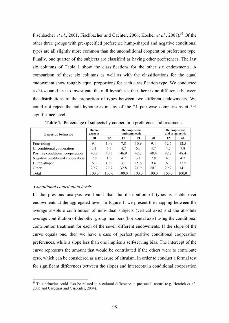
98

Fischbacher et al., 2001, Fischbacher and Gächter, 2006; Kocher et al., 2007).33 Of the

other three groups with pre-specified preference hump-shaped and negative conditional

types are all slightly more common than the unconditional cooperation preference type.

Finally, one quarter of the subjects are classified as having other preferences. The last

six columns of Table 1 show the classifications for the other six endowments. A

comparison of these six columns as well as with the classifications for the equal

endowment show roughly equal proportions for each classification type. We conducted

a chi-squared test to investigate the null hypothesis that there is no difference between

the distributions of the proportion of types between two different endowments. We

could not reject the null hypothesis in any of the 21 pair-wise comparisons at 5%

significance level.

Table 1. Percentage of subjects by cooperation preference and treatment. Homo- geneous

Heterogeneous and symmetric

Heterogeneous and asymmetric Types of behavior

20 12 17 23 28 12 44 Free-riding 9.4 10.9 7.8 10.9 9.4 12.5 12.5 Unconditional cooperation 3.1 6.3 4.7 6.3 4.7 4.7 7.8 Positive conditional cooperation 43.8 40.6 46.9 42.2 48.4 42.2 48.4 Negative conditional cooperation 7.8 1.6 4.7 3.1 7.8 4.7 4.7 Hump-shaped 6.3 10.9 3.1 15.6 9.4 6.3 12.5 Other 29.7 29.7 32.8 21.9 20.3 29.7 14.1 Total 100.0 100.0 100.0 100.0 100.0 100.0 100.0

Conditional contribution levels

In the previous analysis we found that the distribution of types is stable over

endowments at the aggregated level. In Figure 1, we present the mapping between the

average absolute contribution of individual subjects (vertical axis) and the absolute

average contribution of the other group members (horizontal axis) using the conditional

contribution treatment for each of the seven different endowments. If the slope of the

curve equals one, then we have a case of perfect positive conditional cooperation

preferences, while a slope less than one implies a self-serving bias. The intercept of the

curve represents the amount that would be contributed if the others were to contribute

zero, which can be considered as a measure of altruism. In order to conduct a formal test

for significant differences between the slopes and intercepts in conditional cooperation

33 This behavior could also be related to a cultural difference in pro-social norms (e.g. Henrich et al., 2005 and Cardenas and Carpenter, 2004).

99

and altruist levels, we estimate an econometric model. Each individual took 142

conditional decisions for the seven endowments. It is likely that the responses across

decisions are correlated, which suggest that a random effect model should be estimated.

Table 2 presents the results of regressing own conditional contributions on the average

contributions by others, a dummy for each endowment level and an interaction term that

allows different slopes across endowment levels. We take the homogenous endowment,

20, case as the reference point.34 We find that the absolute contribution level increases

with the level of contribution made by others. The slope of conditional contributions is

significantly less than one reflecting some self-serving bias. On average, individuals

contribute significantly more than zero to the public good which reflects a degree of

altruism. The slope of the conditional contribution increases with relative endowment

which means that when subjects are relatively rich, the more others contribute, the more

they contribute themselves. Individuals with higher levels of endowment contribute

more to the public good in an absolute sense than individuals with low levels of

endowment, which is consistent with Buckley and Croson’s (2006) model of altruism

and with empirical findings in Cardenas et al. (2002) and Cherry et al. (2005).

Individuals in the low endowment level contribute significantly less in absolute terms

when they are in a more unequal endowment distribution.

Figure 1. Absolute average conditional contributions.

05

1015

20

0 5 10 15 20Average contribution of others in the group

05

1015

20

0 5 10 15 20Average contribution of others in the group

34 We tried different specifications of the model all with the same basic message.

ei=28 ei=23 ei=17

ei=12

ei=44

ei=20

ei=12

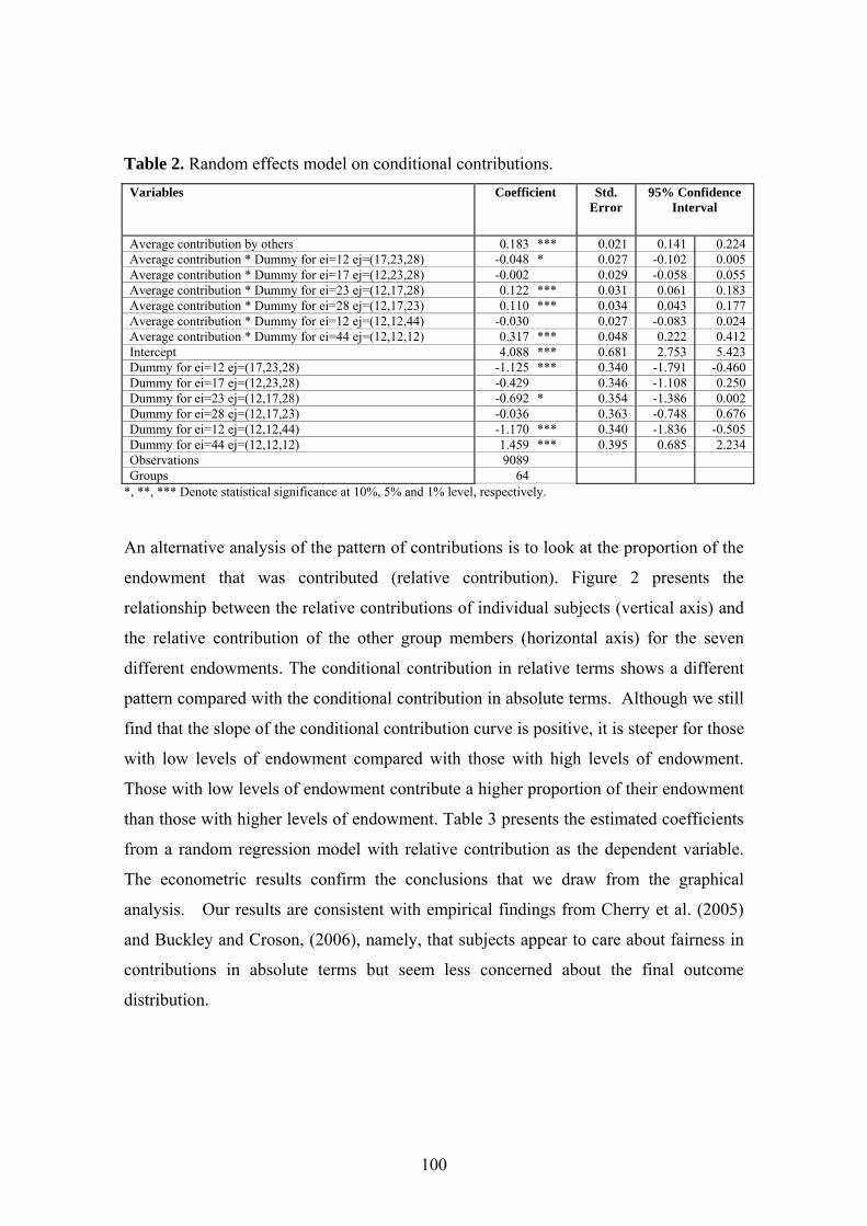
100

Table 2. Random effects model on conditional contributions. Variables Coefficient Std.

Error 95% Confidence

Interval

Average contribution by others 0.183 *** 0.021 0.141 0.224 Average contribution * Dummy for ei=12 ej=(17,23,28) -0.048 * 0.027 -0.102 0.005 Average contribution * Dummy for ei=17 ej=(12,23,28) -0.002 0.029 -0.058 0.055 Average contribution * Dummy for ei=23 ej=(12,17,28) 0.122 *** 0.031 0.061 0.183 Average contribution * Dummy for ei=28 ej=(12,17,23) 0.110 *** 0.034 0.043 0.177 Average contribution * Dummy for ei=12 ej=(12,12,44) -0.030 0.027 -0.083 0.024 Average contribution * Dummy for ei=44 ej=(12,12,12) 0.317 *** 0.048 0.222 0.412 Intercept 4.088 *** 0.681 2.753 5.423 Dummy for ei=12 ej=(17,23,28) -1.125 *** 0.340 -1.791 -0.460 Dummy for ei=17 ej=(12,23,28) -0.429 0.346 -1.108 0.250 Dummy for ei=23 ej=(12,17,28) -0.692 * 0.354 -1.386 0.002 Dummy for ei=28 ej=(12,17,23) -0.036 0.363 -0.748 0.676 Dummy for ei=12 ej=(12,12,44) -1.170 *** 0.340 -1.836 -0.505 Dummy for ei=44 ej=(12,12,12) 1.459 *** 0.395 0.685 2.234 Observations 9089 Groups 64

*, **, *** Denote statistical significance at 10%, 5% and 1% level, respectively.

An alternative analysis of the pattern of contributions is to look at the proportion of the

endowment that was contributed (relative contribution). Figure 2 presents the

relationship between the relative contributions of individual subjects (vertical axis) and

the relative contribution of the other group members (horizontal axis) for the seven

different endowments. The conditional contribution in relative terms shows a different

pattern compared with the conditional contribution in absolute terms. Although we still

find that the slope of the conditional contribution curve is positive, it is steeper for those

with low levels of endowment compared with those with high levels of endowment.

Those with low levels of endowment contribute a higher proportion of their endowment

than those with higher levels of endowment. Table 3 presents the estimated coefficients

from a random regression model with relative contribution as the dependent variable.

The econometric results confirm the conclusions that we draw from the graphical

analysis. Our results are consistent with empirical findings from Cherry et al. (2005)

and Buckley and Croson, (2006), namely, that subjects appear to care about fairness in

contributions in absolute terms but seem less concerned about the final outcome

distribution.

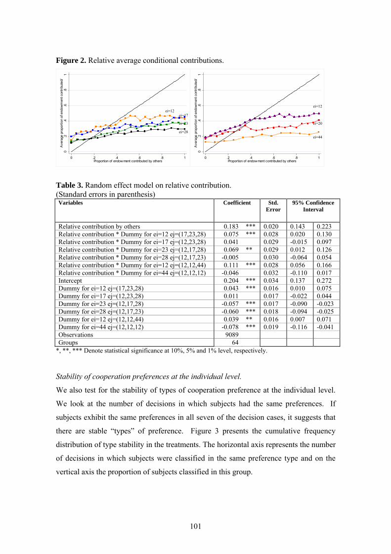
101

Figure 2. Relative average conditional contributions. 0

.2.4

.6.8

1A

vera

ge p

ropo

rtion

of e

ndow

men

t con

tribu

ted/

0 .2 .4 .6 .8 1Proportion of endowment contributed by others

0.2

.4.6

.81

Ave

rage

pro

porti

on o

f end

owm

ent c

ontri

bute

d/

0 .2 .4 .6 .8 1Proportion of endowment contributed by others

Table 3. Random effect model on relative contribution. (Standard errors in parenthesis) Variables Coefficient Std.

Error 95% Confidence

Interval

Relative contribution by others 0.183 *** 0.020 0.143 0.223 Relative contribution * Dummy for ei=12 ej=(17,23,28) 0.075 *** 0.028 0.020 0.130 Relative contribution * Dummy for ei=17 ej=(12,23,28) 0.041 0.029 -0.015 0.097 Relative contribution * Dummy for ei=23 ej=(12,17,28) 0.069 ** 0.029 0.012 0.126 Relative contribution * Dummy for ei=28 ej=(12,17,23) -0.005 0.030 -0.064 0.054 Relative contribution * Dummy for ei=12 ej=(12,12,44) 0.111 *** 0.028 0.056 0.166 Relative contribution * Dummy for ei=44 ej=(12,12,12) -0.046 0.032 -0.110 0.017 Intercept 0.204 *** 0.034 0.137 0.272 Dummy for ei=12 ej=(17,23,28) 0.043 *** 0.016 0.010 0.075 Dummy for ei=17 ej=(12,23,28) 0.011 0.017 -0.022 0.044 Dummy for ei=23 ej=(12,17,28) -0.057 *** 0.017 -0.090 -0.023 Dummy for ei=28 ej=(12,17,23) -0.060 *** 0.018 -0.094 -0.025 Dummy for ei=12 ej=(12,12,44) 0.039 ** 0.016 0.007 0.071 Dummy for ei=44 ej=(12,12,12) -0.078 *** 0.019 -0.116 -0.041 Observations 9089 Groups 64

*, **, *** Denote statistical significance at 10%, 5% and 1% level, respectively.

Stability of cooperation preferences at the individual level.

We also test for the stability of types of cooperation preference at the individual level.

We look at the number of decisions in which subjects had the same preferences. If

subjects exhibit the same preferences in all seven of the decision cases, it suggests that

there are stable “types” of preference. Figure 3 presents the cumulative frequency

distribution of type stability in the treatments. The horizontal axis represents the number

of decisions in which subjects were classified in the same preference type and on the

vertical axis the proportion of subjects classified in this group.

ei=12 ei=17

ei=23

ei=28

ei=12

ei=20

ei=44

102

The most stable types are conditional cooperation, free-riding and un-conditional

cooperation. About one quarter of subjects that exhibit these types of cooperation

preference did so consistently in all seven decisions. Positive conditional cooperation is

the most stable cooperation preference and about 70% of those who exhibited it

remained classified in this preference type for four or more decisions. In contrast only

30% of the free-riders did this. Negative conditional cooperation and hump-shaped

preferences were the most un-stable preferences with only 18% and 9%, respectively, of

the subjects remaining in the same classification for more than four decisions.

Figure 3. Stability of preferences at the individual level.

27% 27%33% 33%

67%

43% 43% 43% 43% 43%

55%

69%

88%

98%

9% 9%

18% 18% 18%

27%

4%9% 9%

13%

35%

18%

33%

61%

79%

29%

24%

12%

0%

10%

20%

30%

40%

50%

60%

70%

80%

90%

100%

012345678

Free-rider Unconditional cooperators

Positive conditional cooperators Negative conditional cooperatorsHump-shaped Other

c

Comparison of contributions in the unconditional and the conditional case.

Besides asking the subjects for their conditional contribution at various levels of

endowment, we also asked for their unconditional contribution and how much they

expected others would contribute. Consistency between unconditional and conditional

decisions implies that we observe similar patterns of behavior. Each person answer how

much they would contribute unconditionally on 7 decisions, responses are likely to be

correlated across decisions, which calls for a random effect model. Table 4 presents the

estimated coefficients from a random effects model with unconditional contribution as

the dependent variable. We take endowment 20 as a reference case.

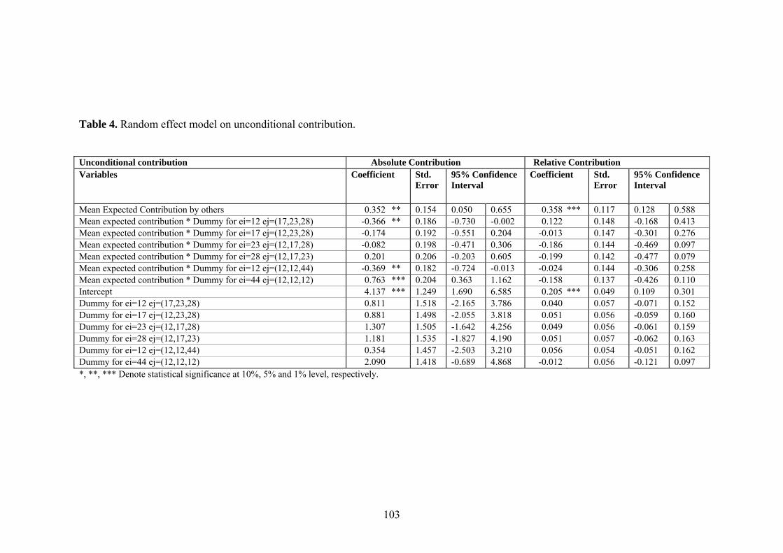
103

Table 4. Random effect model on unconditional contribution.

Unconditional contribution Absolute Contribution Relative Contribution Variables Coefficient Std.

Error 95% Confidence Interval

Coefficient Std. Error

95% Confidence Interval

Mean Expected Contribution by others 0.352 ** 0.154 0.050 0.655 0.358 *** 0.117 0.128 0.588 Mean expected contribution * Dummy for ei=12 ej=(17,23,28) -0.366 ** 0.186 -0.730 -0.002 0.122 0.148 -0.168 0.413 Mean expected contribution * Dummy for ei=17 ej=(12,23,28) -0.174 0.192 -0.551 0.204 -0.013 0.147 -0.301 0.276 Mean expected contribution * Dummy for ei=23 ej=(12,17,28) -0.082 0.198 -0.471 0.306 -0.186 0.144 -0.469 0.097 Mean expected contribution * Dummy for ei=28 ej=(12,17,23) 0.201 0.206 -0.203 0.605 -0.199 0.142 -0.477 0.079 Mean expected contribution * Dummy for ei=12 ej=(12,12,44) -0.369 ** 0.182 -0.724 -0.013 -0.024 0.144 -0.306 0.258 Mean expected contribution * Dummy for ei=44 ej=(12,12,12) 0.763 *** 0.204 0.363 1.162 -0.158 0.137 -0.426 0.110 Intercept 4.137 *** 1.249 1.690 6.585 0.205 *** 0.049 0.109 0.301 Dummy for ei=12 ej=(17,23,28) 0.811 1.518 -2.165 3.786 0.040 0.057 -0.071 0.152 Dummy for ei=17 ej=(12,23,28) 0.881 1.498 -2.055 3.818 0.051 0.056 -0.059 0.160 Dummy for ei=23 ej=(12,17,28) 1.307 1.505 -1.642 4.256 0.049 0.056 -0.061 0.159 Dummy for ei=28 ej=(12,17,23) 1.181 1.535 -1.827 4.190 0.051 0.057 -0.062 0.163 Dummy for ei=12 ej=(12,12,44) 0.354 1.457 -2.503 3.210 0.056 0.054 -0.051 0.162 Dummy for ei=44 ej=(12,12,12) 2.090 1.418 -0.689 4.868 -0.012 0.056 -0.121 0.097 *, **, *** Denote statistical significance at 10%, 5% and 1% level, respectively.

104

The left hand side of the table presents the results for absolute contribution levels and the

right hand side for relative contribution levels. We find that absolute unconditional

contributions increase with average expected contributions by others. One again we

observe self-serving bias as the slope of the conditional contribution curve is less than

one. We find that individuals are willing to contribute positive amounts even if they

expect others to contribute zero which indicates altruism. We find that the slope of the

conditional contribution curve for absolute contributions is larger for higher levels of

endowment compared with low levels of endowment. The level of altruism in absolute

terms does not seem to increase with endowment. We find that the absolute and relative

contributions are significantly different from zero which supports a degree of altruism.

The slope of the relative unconditional contributions increase with the relative expected

contribution by others indicating that conditional cooperation is the dominant type of

behavior. We find that about 20% of the endowment is invested when the expected

contributions by others is zero, which support altruism. Not clear effects are found on the

slope or in altruism with respect to endowment.

An alternative test for consistency is to compare conditional and unconditional

cooperation. By asking subjects how much they expected others in their group to

contribute, it is possible to compare the amount that they decided to contribute in the

unconditional decision with the amount that they contributed in the conditional decision.

Table 5 presents the proportion of answers in which conditional and unconditional

contributions are equal. We also include the proportion of answers where the difference

is only one or two tokens.

Overall, in 27% of the cases there was no difference between answers; in 55% of the

cases the difference was 2 tokens or less. If we study the types separately, free-riders and

unconditional co-operators are the most consistent between the unconditional and

conditional treatments. One explanation of the difference between conditional and

unconditional contribution levels may relate to the fact that the former is a “colder”

approach than directly reporting unconditional contribution levels. There is an on going

debate on this issue and the results are mixed as to whether or not there is a difference

(e.g. Brandts and Charness, 2000; Brosig et al., 2003).

105

Table 5. Proportion of answers where unconditional contribution is equal to conditional

contribution.

Equal One token difference

Two tokens difference

More than two tokens difference

Total

All 27.35 13.90 13.45 45.29 100 Free-Riding 89.36 0.00 2.13 8.51 100 Unconditional Cooperation 56.52 4.35 4.35 34.78 100 Positive Conditional Cooperation 19.60 17.09 17.09 46.23 100 Negative Conditional Cooperation 13.64 9.09 9.09 68.18 100 Hump-shaped 14.63 14.63 17.07 53.66 100 Others 16.67 16.67 13.16 53.51 100

4. Conclusions

The effects of heterogeneous endowments on contribution levels in public goods

experiments have recently received more and more attention in the literature. By

combining the experimental design developed by Fischbacher et al. (2001) with

heterogeneous endowments, we are able to analyze cooperation preferences under the

more realistic case when endowments are heterogeneous within a group. We find that the

most common cooperation preferences are positive conditional co-operators and free-

riders in both the heterogeneous and homogenous cases. This result is in line with

previous findings for homogenous endowments. In addition, we find evidence that

cooperation preferences are stable over heterogeneous endowments. On average,

individuals’ contributions increase with the contributions by others, but they increase less

than proportionally indicating the presence of a self-serving bias. We also find some

evidence to support altruism as motivation behind cooperation since on average

individuals are willing to cooperate even when contribution levels by others are zero.

Moreover, we find evidence that higher endowments increase cooperation in absolute

terms, but decrease it in relative terms. A large degree of internal consistency is found in

the experiment.

Given that cooperative preferences are stable, the results imply that contribution

levels are dependent on the distribution of cooperation preference types i.e. they are

dependent on whether the free-riders or the positive conditional co-operators are on

average richer or poorer within the society.

106

107

5. References Anderson, L.R., J. Mellor and J. Milyo. 2007. “Inequality, group cohesion, and public good provision: An

experimental analysis.” forthcoming in Journal of Socio-Economics. Andreoni, James. 1990. “Impure Altruism and Donations to Public Goods: A Theory of Warm-Glow

Giving.” The Economic Journal, 100(June): 464-477. Andreoni, James. 1995. “Cooperation in public-goods experiments: kindness or confusion?” American

Economic Review. 85 (September): 891–904. Aquino Karl, Victoria Steisel and Avi Kay. 1992. The effects of resource distribution, voice, and decision

framing on the provision of public goods. Journal of Conflict Resolution. 36(4): 665–87. Bergstrom, Theodore C. Laurence E. Blume and Hal Varian. 1986. “On the private Provision of Public

Goods.” Journal of Public Economics. 29 (February):25-49 Bolton, Gary and Axel Ockenfels. 2000. “A theory of equity, reciprocity and competition.” American

Economic Review. 90(March):166-193. Brandts, J. and G. Charness. 2000. "Hot vs. cold: sequential responses and preference stability in

experimental games." Experimental Economics, 2(March): 227-228. Brandts, Jordi and Arthur Schram. 2001. “Cooperation and noise in public goods experiments: applying the

contribution function approach.” Journal of Public Economics, 79 (July): 399–427. Brosig, J., J. Weimann, C.-L. Yang, C.-L. 2000. “The hot versus cold effect in a simple bargaining

experiment." Experimental Economics, 6: 227-228. Buckley, Edward and Rachel Croson. 2006. “Income and wealth heterogeneity in the voluntary

contribution of linear public goods.” Journal of Public Economics 90 (May): 935-955. Cardenas, Juan Camilo and Jeffrey Carpenter. 2004. “Experimental Development Economics: A review of

the Literature and Ideas for Future Research”. Working Paper. Cardenas, Juan Camilo, John Stranlund, Cleve Willis. 2002. “Economic inequality and burden-sharing in

the provision of local environmental quality” Ecological Economics. 40 (March): 379-395. Cardenas, Juan Camilo. 2003. “Real wealth and experimental cooperation: experiments in the field lab.”

Journal of Development Economics. 70 (April):263-289. Chan, Kenneth S., Stuart Mestelman, Rob Moir, R. Andrew Muller 1996. “The voluntary provision of

public goods under varying income distributions.” Canadian Journal of Economics, 96 (February): 54–69.

Chan, Kenneth S., Stuart Mestelman, Rob Moir, R. Andrew Muller 1997. “Equity theory and the voluntary provision of public goods”. Journal of Economic Behavior and Organization. 32 (March): 349-369.

Chan, Kenneth S., Stuart Mestelman, Rob Moir, R. Andrew Muller. 1999. “Heterogeneity and the voluntary provision of public goods.” Experimental Economics. 2(August): 5-30.

Cherry, T., S Kroll and J. Shogren. 2005. “The impact of endowment heterogeneity and origin on public good contributions: evidence from the lab.” Journal of Economic Behavior and Organization. 57(July): 357-65.

Dufwenberg, Martin and Georg Kirchsteiger. 2004. “A theory of sequential reciprocity.” Games and Economic Behavior, 47(May): 268-298.

Fehr, Ernst and Simon Gächter. 2000. “Fairness and Retaliation: The Economics of Reciprocity”, The Journal of Economic Perspectives, 14(Summer): 159-181.

Fehr, Ernst, Schmidt, Klaus M.. 1999. “The theory of fairness, competition, and cooperation.” The Quarterly Journal of Economics. 114(August): 817-868.

Fischbacher, Urs and Simon Gächter. 2006. “Heterogeneous social preferences and the dynamics of free riding in public goods.” Working Paper 2006-01 in CeDEx Discussion Paper Series at The University of Nottingham.

Fischbacher, Urs, Simon Gächter and Ernst Fehr. 2001. “Are people conditionally cooperative? Evidence from a public goods experiment.” Economics Letters. 71(June): 397-404.

Gächter, Simon and E. Renner. 2006. “The effects of (incentivized) belief elicitation in public good experiments,” Working Paper 2006-16 in CeDEx Discussion Paper Series at The University of Nottingham.

Henrich, J., R. Boyd, S. Bowles, H. Gintis, E. Fehr, C. Camerer, R. McElreath, M. Gurven, K. Hill, A. Barr, J. Ensminger, D. Tracer, F. Marlow, J. Patton, M. Alvard, F. Gil-White and N. Henrich. 2005. “Economic Man in Cross-Cultural Perspective: Ethnography and Experiments from 15 small-scale societies.” Behavioral and Brain Sciences, 28, 795-855.

108

Houser, Daniel, Robert Kurzban. 2002. “Revisiting kindness and confusion in public goods experiments.” American Economic Review. 92(September): 1062-1069.

Keser, Claudia and Frans van Winden. 2000. “Conditional cooperation and voluntary contributions to public goods.” Scandinavian Journal of Economics, 102(1), 23-39.

Kocher, Martin, Todd Cherry, Stephan Kroll, Robert Netzer, Mathias Sutter. 2007. “Conditional cooperation in three continents.” Working Papers 2007-02. Faculty of Economics and Statistics, University of Innsbruck.

Kroll, Stephan, Todd L. Cherry and Jason F. Shogren, forthcoming. “The Impact of Endowment Heterogeneity and Origin on Contributions in Best-Shot Public Good Games.” Experimental Economics.

Ledyard, John. 1995. “Public Goods: A survey of experimental research.” In: Kagel, John & Roth, Alvin E.(Eds.), Handbook of Experimental Economics. Princeton: Princeton University Press.

Palfrey, Thomas R. and Jeffrey E. Prisbrey. 1997. “Anomalous behavior in public goods experiments: How much and Why?”. American Economic Review. 87 (December): 829-846.

Van Dijk, Eric, and Henk Wilke. 1994. “Asymmetric of wealth and public good provision.” Social Psychology Quarterly, 57(December): 352-359.

Van Dijk, Eric, and Henk Wilke. 1995. “Coordination rules in asymmetric social dilemmas: a comparison between public good dilemmas and resource dilemmas.” Journal of Experimental Social Psychology, 31(1): 1–27.

Visser, Martine. 2007. “Fairness, Reciprocity and Inequality: Experimental evidence from South Africa.” Dissertation Department of Economics. Göteborg University.

Warr, Peter. 1983. “The private provision of a public good is independent of the distribution of income.” Economics Letters. 13: 207-11

Zelmer, Jennifer. 2003. “Linear public goods experiments: A meta-analysis.” Experimental Economics, 6 (November): 299-310.

109

Appendix A Instructions

You are about to participate in an experiment on decision-making. If you follow these instructions carefully and make good decisions you could earn a considerable amount of money that will be paid to you at the end of this experiment in cash. Throughout the entire experiment, communication of any kind is strictly prohibited. Communication between participants will lead to your exclusion from the experiment and the forfeit of all monetary earnings. If you have any questions, please raise your hand and a member of the research team will come to you and answer your question privately. Your earnings in this experiment will be in “tokens.” At the end of the experiment, tokens will be converted into Euros at the exchange rate of:

2 tokens = 1250 Pesos

Regardless of your decisions in the experiment, you will receive a show-up fee of 7500 Pesos. You will also have to fill in a few questionnaires during the experiment. Some of the questions might seem a bit odd to you; but even so, please, answer them seriously. This is an international research project and we are bound to use the same set of questions in all locations. All your answers remain confidential and anonymous. We will use the experiment number tag that you have received on entering the room to identify you, and this will also be used to identify you when we pay you your income after the experiment.

All participants will bein groups of four. Nobody other than the people running the experiment will know who is in which group.

The Basic Decision

You will now learn how the experiment is conducted. First, we introduce the basic decision-making situation. Then, we ask you to answer control questions that will help you gain an understanding of the decision-making situation.

You will be a member of a group of four people. Groups will be assembled randomly. At the beginning of the experiment you will receive (on paper) an number of tokens called an “endowment”. Each of the four members of a group has to decide how to divide this endowment. You can put all, some or none of your tokens into a group account. Each token you do not deposit in the group account will automatically be transferred to your private account.

110

Different members of your group may have different endowments. You will see on your decision sheet (handed out later) how many tokens you are endowed with and how many tokens are in the endowments of the other members of your group.

Your income from the private account:

For each token you put into your private account, you will earn exactly one token. For example, if you have an endowment of 20 tokens and you put zero tokens into the group account (and therefore 20 tokens in the private account), then you will earn exactly 20 tokens from the private account. If instead you put 14 tokens into the group account (and therefore 6 tokens in the private account), then you receive an income of 6 tokens from the private account. Nobody except you earns tokens from your private account.

Your income from the group account: Everybody receives the same income from the group account that is based on the total number of tokens paid into it by the group. This income is not affected by either the size of an indicual’s endowment or by the amount that an individual puts into the group account. Your income from the group account, therefore will also be earned from the tokens that the other group members put into the group account, not just the tokens that you invest in it yourself. For each group member, the income from the group account will be determined as follows:

Income from the group account = sum of all contributions to the group account x 0.4

For example, if the sum of all contributions to the group account is 60 tokens, you and all other group members will get an income of 60x0.4=24 tokens from the group account. If the four group members deposit a total of 10 tokens in the group account, then you and all others will receive an income of 10x0.4=4 tokens from the group account.

Your total income:

Your total income is the sum of the income from your private account and the income from the group account: Income from your private account (= your endowment – your contribution to the group

account) + Income from the group account (= 0.4 × sum of all contributions to the group account) Total income

Before we finish reading the instructions we will ask you to answer the following control questions that help you to see whether you have understood everything correctly. If there are any questions or problems, please raise your hand. One of the people running the experiment will come to you and answer your questions privately.

111

Control Questions Please answer the following control questions. Their purpose is to make you familiar with calculating the various incomes in tokens that you might arise from the decisions we ask you to make about allocating your endowments. Please answer all questions and write down all calculations. 1. Assume you have an endowment of 23 tokens and the three other group members

have endowments of 12, 17, and 28 tokens each. Assume also that all group members (including yourself) put nothing into the group account.

What is your total income? ____ What are the incomes of the three other group members? ____, ____, and ____

2. Assume you have an endowment of 23 tokens and the three other group members

have endowments of 12, 17, and 28 tokens each. Assume also that all group members (including yourself) put their entire endowment into the group account.

What is your total income? ____ What are the incomes of the three other group members?____, ____, and ____

3. Assume you have an endowment of 23 tokens. Assume also that the other group

members collectively put a total of 30 tokens into the group account.

a) What is your total income, if you, in addition to the 30 tokens of the other 3 group members, put 0 tokens into the group account? Your total income: ____

b) What is your total income, if you, in addition to the 30 tokens of the other 3 group

members, put 8 tokens into the group account? Your total income: ____

c) What is your total income, if you, in addition to the 30 tokens of the other 3 group

members, put 15 tokens into the group account? Your total income: ____

4. Assume you have an endowment of 23 tokens. You put 9 tokens into the group

account.

112

a) What is your total income, if the other group members, in addition to your 9 tokens, put another 7 tokens into the group account?

Your total income: ____

b) What is your total income, if the other group members, in addition to your 9

tokens, put another 12 tokens into the group account?

Your total income: ____ c) What is your total income, if the other group members, in addition to your 9

tokens, put another 22 tokens into the group account?

Your total income: ____ If you finish these questions before the others, we advise you to think about additional examples to familiarize yourself further with these types of decision-making situations. The Experimental procedure The experiment consists of decision-making situations like the one that we have just described. In the following we explain the procedure in detail.

As you know you have an endowment of tokens. You can put these tokens into a group account and the remaining tokens will automatically be deposited into your private account. Each member of your group may have a different number of tokens in his or her endowment.

Each group member has to make two types of decision. In the following instructions, we will refer to them as the “unconditional contribution” and the “contribution table decision.” • With the unconditional contribution to the group account, you decide how many of the tokens in your endowment to put into the group account. Write this amount behind “Your unconditional contribution to the group account” on the first page of your decision sheet. You must write down an integer number that cannot be smaller than zero or larger than the total number of tokens that you have been given in your endowment. The difference between your endowment and the amount you put into the group account is automatically the amount that will go into your private account. • Your second task is to fill out a contribution table on page 2 of the decision sheet. In the contribution table you have to indicate how many tokens you would like to put into the group account for each possible average contribution of the other three group members (rounded up or down to the next integer number). What you actually contribute

113

will depend on what the other group members actually contribute. This will become clear to you when you see the following contribution table example:

(Rounded) Average contribution of the

other group members to the group account

Your contribution to the group account is

0 1 2 3 4 5 6 7 8 9

10 11 12 13 14 15 16 17 18 19

The numbers in the left column are the possible (rounded) average contributions of the other group members. Assume for this example that the other group members have endowments of 12, 17 and 28 and can therefore contribute on average a maximum of 19 tokens (= (12+17+28)/3). Your actual contribution table might have a larger or smaller number of rows, depending on the sizes of endowment of the other group members (remember that different group members may have different sizes of endowment). Using the column on the right, you simply have to write down how many tokens you would like to contribute to the group account for each possible average contribution of the others. You must make an entry in each field of the right column. For example, you must write down how many tokens you want to contribute to the group account if the others contribute on average 0 tokens to the group account; how many you contribute if the others contribute 1 or 2 or 3 tokens, etc. In each field, you must write down an integer a number that is neither smaller than zero and nor larger than the total number of tokens in your endowment. You can, of course, write down the same number in different fields. After all participants of the experiment have made their unconditional contribution decisions and have filled out their conditional contribution table, one member of each

114

group will be selected randomly. Each person will receive payment for one decision only and this random selection mechanism is used to determine whether it is the unconditional contribution decision or the contribution table decision that is paid. For the randomly selected group member, only the contribution table will be income-relevant. For the other 3 group members that are not selected, the unconditional contribution decision will be the income-relevant decision. When you make your unconditional contribution and when you fill out the contribution table you do not know whether you will be selected randomly. Therefore you will have to think carefully about both types of decision because both could affect the amount that you earn. The following two examples should illustrate this: Example 1: Assume that after you have handed in your decisions you have been selected by the random mechanism. This implies that your income-decision will be the contribution table. For the other 3 group members the unconditional contribution is the relevant decision. Assume they have made unconditional contributions of 0, 2, and 5 tokens. The rounded average contribution is therefore 2 (7/3 = 2.33). If you have indicated in your contribution table that you will put one token into the group account if the others contribute 2 tokens on average, then the total contribution to the group account is 0+2+5+1=8. Thus all group members earn an income of 0.4x8=3.2 from the group account plus the respective incomes from their private accounts. If you have indicated instead that you will contribute 19 tokens to the group account if the others contribute 2 on average, then the total contribution to the group account is 0+2+5+19=26. All group members earn an income of 0.4x26=10.4 tokens from the group account plus the respective incomes from their private accounts. Example 2: Now assume that you have not been selected by the random mechanism, which means that for you and two other group members the unconditional contribution is the income-relevant decision. Assume further that your unconditional contribution to the group account is 16, and that those of the other two group members are 18 and 20 each. The average unconditional contribution of you and the other two is therefore 18 (=16+18+20)/3). If the randomly selected group member indicates in the contribution table that he or she contributes one token to the group account when the other 3 group members contribute 18 on average, then the total contribution of the group to the group account is 16+18+20+1=55 tokens. All group members will therefore earn 0.4x55=22 tokens form the group account in addition to the respective incomes from their private accounts. If the randomly selected group member instead indicated in the contribution table that he or she will contribute 19 tokens to the group account when the other 3 group members contribute 18 on average, then the total contribution of the group to the group account is 16+18+20+19=73 tokens. All group members will therefore earn 0.4x73=29.2 tokens from the group account in addition to the respective incomes from their private accounts. The random selection of the participants will be implemented as follows. Each group member is assigned the name of a playing card (Jack, Queen, King or Ace) that can be seen on you’re his or her decision sheet. After all of the participants have made their unconditional contribution and contribution table decisions, a randomly selected participant will draw one of four playing cards (Jack, Queen, King, Ace),. If the card that

115

is drawn matches the card on your decision sheet, then your payment will be based on the contribution table on page 2 of your decision sheet. Otherwise, your payment will be for your unconditional contribution on page 1. Remember that you only know which decision your payment will be based on after you have submitted your decisions. Thus, you should fill out both pages carefully. The following graph is a visual presentation of the situation from example 1. You are the person to the right, whose card is an Ace (A). An A was drawn in the random selection mechanism and therefore page 2 of the decision sheet is the relevant page for you, while page 1 is the relevant page for everybody else. While all group members had to fill out both pages completely (indicated by the letter “x”) only the decisions in bold are relevant to the payoff.

Seven parallel decisions:

In the experiment, you are simultaneously in nine groups that are randomly assembled from the people in that room. Each consists of four members. You do not know and will never get to know the other group members, and they do not know and will never get to know that you were in their group. You have to fill out seven decision sheets ,each with an unconditional contribution on p. 1 and a conditional contribution on page 2. You do not have to fill out nine decision sheets because for three of the groups, you have exactly the same endowment so that we can take your values from one decision sheet only).

The decision sheets do not have to be completed in any particular order. In a minute we will hand out your decision sheets, and you can start with any one of them. You can also go back and make corrections on a sheet that you already filled out if you wish. When you have filled out all seven sheets, we will come and collect them from you. The only difference between the seven decisions sheets, i.e. the seven groups in which you

J Contr.

Of Others

Your Cont.

0 x 1 x 2 x 3 x … x 20 x

2

Q Contr.

Of Others

Your Cont.

0 x 1 x 2 x 3 x

… x 20 x

2

K Contr.

Of Others

Your Cont.

0 x 1 x 2 x 3 x

… x 20 x

2

Q Your Unconditional Contribution: 2

1

J Your Unconditional Contribution: 0

1

K Your Unconditional Contribution: 5

1

A Your Unconditional Contribution: x

A Contr.

Of Others

Your Cont.

0 x 1 x 2 1 3 x … x 20 x

2

116

are placed, is that the distribution of endowments within the group is different. So take a close look at the top of the sheets to discern this potentially important information. If you have any problems or questions at any time during the experiment, please raise your hand.

At the end of the experiment, your payment will be determined by randomly selecting one of the nine groups to which you belong. We will let one of you draw a lottery ticket at the end of the experiment out of a basket that contains nine tickets that are colored red, yellow, blue, green, black, white, orange, purple and pink (the names of the nine groups). The number of tokens that you earned in the group that selected in the draw will then be converted into Euros and paid to you in cash. The other eight groups do not result in cash payments. Since you do not know which group is going to be selected for the payoff, we advise you to think seriously about all your decisions because any one of them could influence your payoff. Therefore, please take your time in filling out the decision sheets.

Do you have any questions? Please raise your hand if you do and a member of the research team will come to you and answer your question privately.

117

Experiment ID:______  Your card in your groups (Jack, Queen, King or Ace):___  Group Red 

Decision Sheet Page 1

Your endowment: 20 tokens

Endowment of player 2: 20 tokens Endowment of player 3: 20 tokens Endowment of player 4: 20 tokens

Your unconditional contribution to the group account: ______ (it must be an integer number not smaller than 0 and not larger than 20)

118

Page 2

Your conditional contribution to the group account (contribution table decision):

(Please enter in the cells of the right-hand column the number of tokens you want to contribute to the group account, given the average contributions of the other group members to the group account in the left column of the same row. As before, you must enter integer numbers.)

(Rounded) Average contribution of the

other group members to the group account

Your contribution to the group account is

0 1 2 3 4 5 6 7 8 9

10 11 12 13 14 15 16 17 18 19 20

119

How many tokens do you think others in your group have unconditionally contributed to the group account?

Earlier, you were asked to fill out 7 sheets with one unconditional contribution and a number of conditional contributions. Now we ask you to state what you believe the other participants in your groups have written down for their unconditional contribution.

Please record the number of tokens you believe the other 3 players in each of the 7 groups to have contributed unconditionally to the group account. In other words, what number do you think each of them wrote down on page 1? The range of possible contributions to the group account for each member varies from group to group. Please refer to the possible contribution amounts (found in parentheses) in the relevant cells of the [table on expected contributions. For example, each member in Group Red can contribute between 0 and 20 tokens; player 2 of group Yellow can contribute between 0 and 17 tokens, and so on.

Remember that one group will be selected randomly in order to determine the payments. You will earn money from the allocation as described in the instruction for the randomly selected group AND you can now earn more money if your beliefs for the selected group are correct. Suppose Group Green is selected randomly. You can then earn an additional 2 tokens for each of your beliefs that is no more than one token larger or smaller than the actual contribution of a member of Group Green to the group account. Suppose you guessed 10 tokens for player 2, 5 tokens for player 3 and 10 tokens for player 4, and the actual choices of the three players were 11, 4 and 5 tokens, respectively. Then you would earn an additional 4 tokens because your guesses for players 1 and 3 would have been close enough to the actual values. Note that players in your group will be assigned player numbers randomly so that you can refer to them easily.

120

Expected contributions to the group account Group Red Group Yellow Group Blue Group Green Group Black Groups

White/Purple/PinkGroup Orange

Your endowment

Endowment: 20

Endowment: 12

Endowment: 17

Endowment: 23

Endowment: 28

Endowment: 12 Endowment: 44

Player 2 Endowment: 20

Endowment: 17

Endowment: 12

Endowment: 12

Endowment: 12

Endowment: 12 Endowment: 12

Expect.:

__________ (0 – 20)

Expect.:

__________ (0 – 17)

Expect.:

__________ (0 – 12)

Expect.:

__________ (0 – 12)

Expect.:

__________ (0 – 12)

Expect.:

__________ (0 – 12)

Expect.:

__________ (0 – 12)

Player 3

Endowment:

20

Endowment:

23

Endowment:

23

Endowment:

17

Endowment:

17

Endowment: 12

Endowment:

12 Expect.:

__________

(0 – 20)

Expect.:

__________ (0 – 23)

Expect.:

__________ (0 – 23)

Expect.:

__________ (0 – 17)

Expect.:

__________ (0 – 17)

Expect.:

__________ (0 – 12)

Expect.:

__________ (0 – 12)

Player 4

Endowment:

20

Endowment:

28

Endowment:

28

Endowment:

28

Endowment:

23

Endowment: 44

Endowment:

12 Expect.:

__________

(0 – 20)

Expect.:

__________ (0 – 28)

Expect.:

__________ (0 – 28)

Expect.:

__________ (0 – 28)

Expect.:

__________ (0 – 23)

Expect.:

_________ (0 – 44)

Expect.:

__________ (0 – 12)

121