SMS NOTES 1st UNIT 8th Sem

8/8/2019 SMS NOTES 1st UNIT 8th Sem

http://slidepdf.com/reader/full/sms-notes-1st-unit-8th-sem 1/30

CHAPTER - 1: INTRODUCTION TO SIMULATION

A Model is a representation of an object, a system, or an idea in some form other than

that of the entity itself.

• This model takes the form of a set of assumptions concerning the operation of the system.

• The assumptions are expressed in:

1. Mathematical relationships

2. Logical relationships &

3. Symbolic relationships between the entities of the system.

• The model solved by mathematical methods such as differential calculus, probability

theory, algebraic methods has the solution usually consists of one or more numerical

parameters which are called measures of performance.

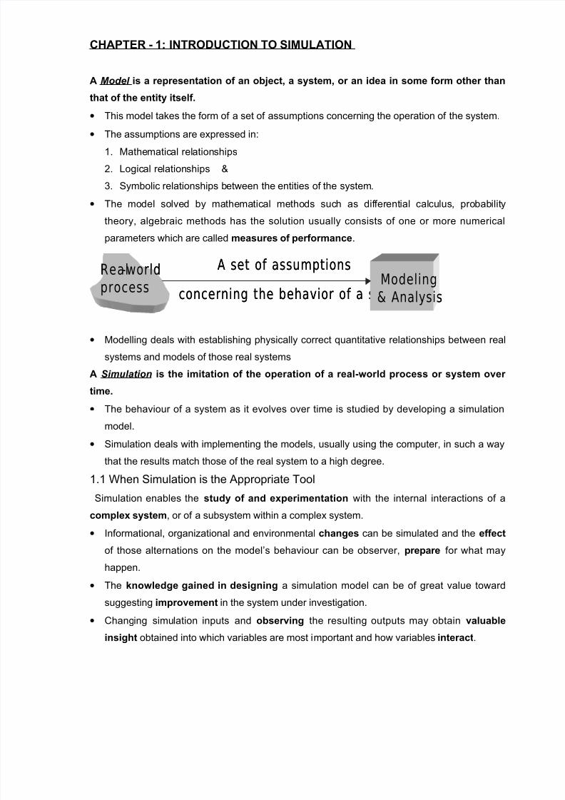
• Modelling deals with establishing physically correct quantitative relationships between real

systems and models of those real systems

A Simulation is the imitation of the operation of a real-world process or system over

time.

• The behaviour of a system as it evolves over time is studied by developing a simulation

model.

• Simulation deals with implementing the models, usually using the computer, in such a way

that the results match those of the real system to a high degree.

1.1 When Simulation is the Appropriate Tool

Simulation enables the study of and experimentation with the internal interactions of a

complex system, or of a subsystem within a complex system.

• Informational, organizational and environmental changes can be simulated and the effect

of those alternations on the model’s behaviour can be observer, prepare for what may

happen.

• The knowledge gained in designing a simulation model can be of great value toward

suggesting improvement in the system under investigation.

• Changing simulation inputs and observing the resulting outputs may obtain valuable

insight obtained into which variables are most important and how variables interact.

Real-worldprocess concerning the behavior of a system

A set of assumptionsModeling& Analysis

Real-worldprocess concerning the behavior of a system

A set of assumptionsModeling& Analysis



• Simulation can be used as an instructive strategical device to reinforce analytic solution

methodologies.

• Simulation can be used to verify analytic solutions.

• By simulating different capabilities for a machine, requirements can be determined.

• Simulation models designed for training, allow learning without the cost and disruption of

on-the-job learning.

• Animation shows a system in simulated operation so that the plan can be visualized.

• The modern system (factory, water fabrication plant, service organization, etc) is so

complex that the interactions can be treated only through simulation.

1.2 When Simulation is Not Appropriate

•

Simulation should not be used when the problem can be solved using common sense. • Simulation should not be used if the problem can be solved analytically.

• Simulation should not be used, if it is easier to perform direct experiments.

• Simulation should not be used, if the costs exceed savings.

• Simulation should not be performed, if the resources or time are not available.

• If no data is available, not even estimate simulation is not advised.

• If managers have unreasonable expectations say, too much soon – or the power of

simulation is over estimated, simulation may not be appropriate.

• If system behaviour is too complex or cannot be defined, simulation is not appropriate.

1.3 Advantages of Simulation

• When mathematical analysis methods are not available, simulation may be the only

investigation tool

• When mathematical analysis methods are available, but are so complex that simulation

may provide a simpler solution

• Allows comparisons of alternative designs or alternative operating policies

• Allows time compression or expansion

• New policies, operating procedures, decision rules, information flows, organizational

procedures etc., can be explored without real systems

• New hardware designs, physical layouts, transportation systems, etc., can be tested

• Hypothesis about how or why

• Insight can be obtained about the interaction and importance of variables

• Bottleneck analysis can be performed

• Useful for design of new systems



1.4 Disadvantages of simulation

• Model building requires special training.

• Simulation results may be difficult to interpret.

•

Simulation modelling and analysis can be time consuming and expensive.• Simulation is used in some cases when an analytical solution is possible or even

preferable.

1.5 Applications of Simulation

1. Manufacturing facility

2. Bank operation

3. Airport operations (passengers, security, planes, crews, baggage)4. Transportation/logistics/distribution operation

5. Hospital facilities (emergency room, operating room, admissions)

6. Computer network

7. Business process (insurance office)

8. Criminal justice system

9. Chemical plant

10.Fast-food restaurant

11.Supermarket

12.Theme park

13. Emergency-response system

14.Designing and analysing manufacturing systems

15.Evaluating H/W and S/W requirements for a computer system

16.Evaluating a new military weapons system or tactics

17.Determining ordering policies for an inventory system

18.Designing communications systems and message protocols for them

19.Designing and operating transportation facilities such as freeways, airports, subways, or

ports

20.Evaluating designs for service organizations such as hospitals, post offices, or fast-food

restaurants

21.Analysing financial or economic systems

1.6 Systems



A system is defined as an aggregation or assemblage of objects joined in some regular

interaction or interdependence toward the accomplishment of some purpose. Systems –

facility or process, actual or planned

Example: Production System

In the above system there are certain distinct objects, each of which possesses properties of

interest. There are also certain interactions occurring in the system that cause changes in the

system.

System Environment

• Changes occurring outside the system.

• The decision on the boundary between the system and its environment may depend on

the purpose of the study

1.7 Components of a System

Entity

An entity is an object of interest in a system.

Ex: In the factory system, departments, orders, parts and products are The entities.

Attribute

An attribute denotes the property of an entity.

Ex: Quantities for each order, type of part, or number of machines in a Department are

attributes of factory system.

Activity

Any process causing changes in a system is called as an activity.

Ex: Manufacturing process of the department.

State of the System

The state of a system is defined as the collection of variables necessary to describe a system

at any time, relative to the objective of study. In other words, state of the system mean a

description of all the entities, attributes and activities, as they exist at one point in time.

Event



An event is defined as an instantaneous occurrence that may change the state of the system.

1.8 System Environment

• The external components that interact with the system and produce necessary changes are

said to constitute the system environment.

• Ex: In a factory system, the factors controlling arrival of orders may be considered to be

outside the factory but yet a part of the system environment. When, we consider the

demand and supply of goods, there is certainly a relationship between the factory output

and arrival of orders. This relationship is considered as an activity of the system.

Endogenous System

The term endogenous is used to describe activities and events occurring within a system.

Ex: Drawing cash in a bank.

Exogenous System

The term exogenous is used to describe activities and events in the environment that affect

the system. Ex: Arrival of customers.

Closed System

A system for which there is no exogenous activity and event is said to be a closed. Ex: Water

in an insulated flask.

Open system

A system for which there is exogenous activity and event is said to be an open. Ex: Bank

system.

Discrete and Continuous Systems

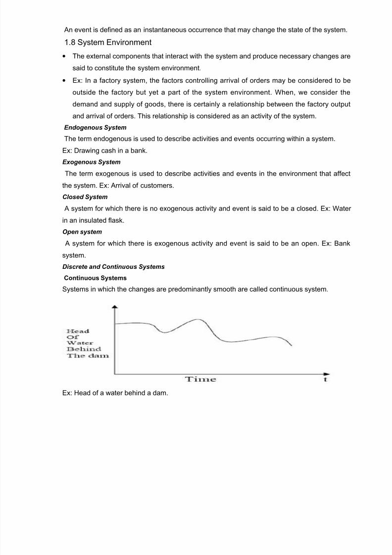
Continuous Systems

Systems in which the changes are predominantly smooth are called continuous system.

Ex: Head of a water behind a dam.



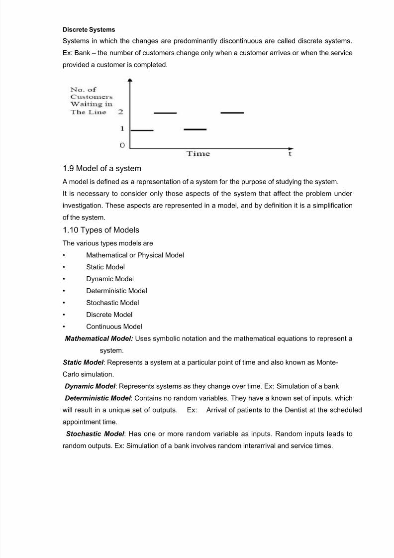
Discrete Systems

Systems in which the changes are predominantly discontinuous are called discrete systems.

Ex: Bank – the number of customers change only when a customer arrives or when the service

provided a customer is completed.

1.9 Model of a systemA model is defined as a representation of a system for the purpose of studying the system.

It is necessary to consider only those aspects of the system that affect the problem under

investigation. These aspects are represented in a model, and by definition it is a simplification

of the system.

1.10 Types of Models

The various types models are

• Mathematical or Physical Model• Static Model

• Dynamic Model

• Deterministic Model

• Stochastic Model

• Discrete Model

• Continuous Model

Mathematical Model: Uses symbolic notation and the mathematical equations to represent asystem.

Static Model : Represents a system at a particular point of time and also known as Monte-

Carlo simulation.

Dynamic Model : Represents systems as they change over time. Ex: Simulation of a bank

Deterministic Model : Contains no random variables. They have a known set of inputs, which

will result in a unique set of outputs. Ex: Arrival of patients to the Dentist at the scheduled

appointment time.

Stochastic Model : Has one or more random variable as inputs. Random inputs leads to

random outputs. Ex: Simulation of a bank involves random interarrival and service times.



Discrete and Continuous Model : Used in an analogous manner. Simulation models may be

mixed both with discrete and continuous. The choice is based on the characteristics of the

system and the objective of the study.

1.11 Discrete-Event System Simulation

• Modelling of systems in which the state variable changes only at a discrete set of points in

time.

• The simulation models are analysed by numerical rather than by analytical methods.

• Numerical methods use computational procedures and are ‘runs’, which is generated

based on the model assumptions and observations are collected to be analysed and to

estimate the true system performance measures.

• Real-world simulation is so vast, whose runs are conducted with the help of computer.

Much insight can be obtained by simulation manually, which is applicable for small

systems.

1.12 Steps in a Simulation study

1. Problem formulation

Every study begins with a statement of the problem, provided by policy makers. Analyst

ensures it’s clearly understood. If analyst develops it, policy makers should understand and

agree with it.

2. Setting of objectives and overall project plan

The objectives indicate the questions to be answered by simulation. At this p

determination should be made concerning whether simulation is the appropriate methodology.

Assuming it is appropriate, the overall project plan should include

• A statement of the alternative systems

• A method for evaluating the effectiveness of these alternatives

• Plans for the study in terms of the number of people involved

• Cost of the study

• The number of days required to accomplish each phase of the work with the anticipated

results.

3. Model conceptualisation

The construction of a model of a system is probably as much art as science.

The art of modelling is enhanced by ability:

• To abstract the essential features of a problem

• To select and modify basic assumptions that characterize the system

• To enrich and elaborate the model until a useful approximation results



Thus, it is best to start with a simple model and build toward greater complexity. Model

conceptualisation enhances the quality of the resulting model and increases the confidence of

the model user in the application of the model.

4. Data collection

There is a constant interplay between the construction of model and the collection of needed

input data. Done in the early stages. Objective kind of data is to be collected.

5. Model translation

Real-world systems result in models that require a great deal of information storage and

computation.

Simulation languages are powerful and flexible.

Simulation software models development time can be reduced.

6. Verified

It pertains to he computer program and checking the performance. If the input parameters and

logical structure and correctly represented, verification is completed.

7. Validated

It is the determination that a model is an accurate representation of the real system. Achieved

through calibration of the model, an iterative process of comparing the model to actual system

behaviour and the discrepancies between the two.

8. Experimental Design

The alternatives that are to be simulated must be determined. Which alternatives to simulate

may be a function of runs? For each system design, decisions need to be made concerning

• Length of the initialisation period

• Length of simulation runs

• Number of replication to be made of each run

9. Production runs and analysis

They are used to estimate measures of performance for the system designs that are being

simulated.10. More runs

Based on the analysis of runs that have been completed. The analyst determines if additional

runs are needed and what design those additional experiments should follow.

11. Documentation and reporting

Two types of documentation.

• Program documentation

• Process documentation



Program documentation

Can be used again by the same or different analysts to understand how the program operates.

Further modification will be easier. Model users can change the input parameters for better

performance.

Process documentation

Gives the history of a simulation project. The result of all analysis should be reported clearly

and concisely in a final report. This enable to review the final formulation and alternatives,

results of the experiments and the recommended solution to the problem. The final report

provides a vehicle of certification.

12. Implementation

Success depends on the previous steps. If the model user has been thoroughly involved and

understands the nature of the model and its outputs, likelihood of a vigorous implementation is

enhanced.

The simulation model building can be broken into 4 phases.

I Phase

• Consists of steps 1 and 2

• It is period of discovery/orientation



• The analyst may have to restart the process if it is not fine-tuned

• Recalibrations and clarifications may occur in this phase or another phase.

II Phase

• Consists of steps 3,4,5,6 and 7

• A continuing interplay is required among the steps



• Exclusion of model user results in implications during implementation

III Phase

• Consists of steps 8,9 and 10

• Conceives a thorough plan for experimenting

• Discrete-event stochastic is a statistical experiment

• The output variables are estimates that contain random error and therefore proper statistical

analysis is required.

IV Phase

• Consists of steps 11 and 12

• Successful implementation depends on the involvement of user and every steps successful

completion.

CHAPTER - 2: SIMULATION EXAMPLES

• Simulation is often used in the analysis of queuing models.

• Three steps of the simulations:



1. Determine the characteristics of each of the inputs to the simulation. -Modelled as

probability distributions, either continuous or discrete.

2. Construct a simulation table.

3. For each repetition i, generate a value for each of the p inputs, and evaluate the

function, calculating a value of the response y i. The input values may be computed by

sampling values from the distributions determined in step 1. A response typically

depends on the inputs and one or more previous responses.

Repetitions Xi1 Xi2 … Xip ResponseYi

1

2

3

:

N

• In a simple typical queuing model, shown in fig 1, customers arrive from time to time and join

a queue or waiting line, are eventually served, and finally leave the system.

Figure 1: Simple Queuing model

The term "customer" refers to any type of entity that can be viewed as requesting "service"from a system.

2.3 Simulation of Queuing systems

• The calling population, nature of arrivals, service mechanism, system capacity and thequeuing mechanism, describes a queuing system

• In the single-channel queue, the calling population is infinite.

• If a unit leaves the calling population and joins the waiting line or enters service, there is nochange in the arrival rate of other units that may need service.

• Arrivals for service occur one at a time in a random fashion.

•

Once they join the waiting line, they are eventually served.• Service times are of some random length according to a probability distribution, which

does not change over time.

• The system capacity has no limit, meaning that any number of units can wait in line.

• A single server or channel serves the units in the order of their arrival.

• Arrivals and services are defined by the distribution of the time between arrivals and thedistribution of service times, respectively.

• Total arrival rate < total service rate

• In some systems, the condition about arrival rate being less than service rate may notguarantee stability

• System state: number of units, server idle or busy

• Events: Set of circumstances that cause instantaneous changes

• Simulation Clock: used to track simulated time

• If a unit has just completed service, the simulation proceeds in the manner shown in theflow diagram of Figure 2

Calling populationWaiting Line

Serv

Calling populationWaiting Line

Serv



• Note that the server has only two possible states: it is either busy or idle.

Figure 2: Service-just-completed flow diagram

• The arrival event occurs when a unit enters the system.

• The unit may find the server either idle or busy.

1. Idle: the unit begins service immediately

2. Busy: the unit enters the queue for the server.

Figure 3: Unit-Entering system flow diagram

• After the completion of a service the service may become idle or remain busy with the nextunit.

• If the queue is not empty, another unit will enter the server and it will be busy. If the queueis empty, the server will be idle after a service is completed.

• It is impossible for the server to become busy if the queue is empty when a service iscompleted.

• Similarly, it is impossible for the server to be idle after a service is completed when thequeue is not empty.

Departure

Event

Remove the waiting unit

from the queue

Begin servicing the unit

Begin server

idle time

Another unit

waiting?

YesNo

Departure

Event

Remove the waiting unit

from the queue

Begin servicing the unit

Begin server

idle time

Another unit

waiting?

YesNo

Arrival

Event

Serverbusy?

Unit enters queue

for service

Unit enters

service

YesNo

Arrival

Event

Serverbusy?

Unit enters queue

for service

Unit enters

service

YesNo



• Simulations of queuing systems generally require the maintenance of an event list for determining what happens next.

• Simulation clock times for arrivals and departures are computed in a simulation tablecustomized for each problem.

• In simulation, events usually occur at random times, the randomness imitating uncertaintyin real life.

• Random numbers are distributed uniformly and independently on the interval (0, 1).• Random digits are uniformly distributed on the set {0, 1, 2, … , 9}.

• The proper number of digits is dictated by the accuracy of the data being used for inputpurposes.

• Pseudo-random numbers: the numbers are generated using a procedure detailed inChapter 7.

• Calculation of IAT: Assume that rolling a die five times and recording the up face generatedthe time between arrivals.

Table 1: Interarrival and Clock Times

• Calculation of ST: The only possible service times are one, two, three, and four time units.

• Assuming that all four values are equally likely to occur, these values could have beengenerated by placing the numbers one through four on chips and drawing the chips from ahat with replacement, being sure to record the numbers selected.

• The interarrival times and service times must be meshed to simulate the single channelqueuing system



Table 2: Simulation Table emphasizing Clock Times

• Table 2 was designed specifically for a single-channel queue, which serves customers on a

FIFO basis. It keeps track of the clock time at which each event occurs.

• The second column records the clock time of each arrival event, while the last columnrecords the clock time of each departure event.

Chronological ordering of events:

The number of customers in the system at the various clock times:

191966DepartureDeparture

151566ArrivalArrival



9955ArrivalArrival


7744ArrivalArrival

6633ArrivalArrival


2222ArrivalArrival


0011ArrivalArrival

Clock TimeClock TimeCustomer Number Customer Number Event TypeEvent Type


151566ArrivalArrival



9955ArrivalArrival


7744ArrivalArrival

6633ArrivalArrival


2222ArrivalArrival


0011ArrivalArrival

Clock TimeClock TimeCustomer Number Customer Number Event TypeEvent Type



EXAMPLE 1: Single-Channel Queue

Assumptions

•Only one checkout counter.•Customers arrive at this checkout counter at random from 1 to 8 minutes apart. Each possiblevalue of interarrival time has the same probability of occurrence.•The service times vary from 1 to 6 minutes.•The problem is to analyze the system by simulating the arrival and service of 20 customers.

Table 3: Distribution of time between arrivals

Table 4: Service Time distribution

A set of uniformly distributed random numbers is needed to generate the arrivals at thecheckout counter. Random numbers have the following properties:1. The set of random numbers is uniformly distributed between 0 and 1.2. Successive random numbers are independent.

Checkout Counter

Arrival Departure



Table 5: Time between arrivals determination

Table 6: Service Times Generated

The essence of a manual simulation is the simulation table, where measures of performancecan be obtained.Table 8: Simulation Table for the queuing problem



1. The average waiting time for a customer is 2.8minutes. This is determined in the followingmanner:

2. The probability that a customer has to wait in the queue is 0.65. This is determinedin the following manner:

3. The fraction of idle time of the server is 0.21. This is determined in the following manner:

4. The average service time is 3.4 minutes, determined as follows:

This result can be compared with the expected service time by finding the mean of the service-time distribution using the equation

The expected service time is slightly lower than the average time in the simulation. The longer simulation, the closer the average will be to E (S).5. The average time between arrivals is 4.3 minutes. This is determined in the followingmanner:

This result can be compared to the expected time between arrivals by finding

of the discrete uniform distribution whose endpoints are a = 1 and b = 8.

6. The average waiting time of those who wait is 4.3 minutes. This is determined in the

following manner: 7. The average time a customer spends in the system is 6.2 minutes. This can be determined

in two ways. First, the computation can be achieved by the following relationship:The second way of computing this same result is to realize that the following relationship

must hold:Average time customer average time customer average t

Spends in the system = spends waiting in the queue + spends in serviceFrom findings 1 and 4 this results in:

Average time customer spends in the system = 2.8+ 3.4 = 6.2 minutes.

EXAMPLE 2: - The Able Baker Call Centre Problem Assumptions

(min)8.220

56===

customersof numberstotal

queueinwait customerstimetotal timewaitng average

65.02013)( ===

customersof numberstotal wait whocustomersof number wait yprobabilit

21.086

18===

simulationof timeruntotal

server of timeidletotal server idleof yprobabilit

(min)4.320

68===


timeservicetotal timeserviceaverage

∑∞

=

=0

)()(s

sspS E

(min)2.3)05.0(6)10.1(5)25.0(4)30.0(3)20.0(2)10.0(1)( =+++++=S E

(min)3.419

82

1==

−

=

arrivalsof numbers

arrivalsbetweentimesall of sumarrivalsbetweentimeaverage

(min)5.42

81

2)( =

+=

+=

baAE

(min)3.413

56===

wiat whocustomersof numberstotal

queueinwait customerstimetotal wait whothoseof timewaiting average

(min)2.620

124===


systeminspend customerstimetotal systemtheinspendscustomer timeaverage



• Consider a computer technical support centre where personnel take calls and provideservice.

• The tome between call ranges from 1 to 4.

• Two technical supports Able and Baker are there. Able is more experienced & can provideservice faster than Baker.

• The distribution of their service times is shown below.Table 8: Interarrival distribution of calls for technical support

• A simplifying rule is that Able gets the customer if both carhops are idle.

Table 9 & 10: Service distribution of Able & Baker

Table 11: Simulation table for Call Centre Problem



After the first customer, the cells for the other customers must be based on logic and formulas.For example, the “clock time of arrival” in the row for the second customer is computed asfollows: D2 = D1+C2

The analysis of table results in the following:

1. Over the 62-minute period able was busy 90% of the time.2. Baker was busy only 69% of the tome. The seniority rule keeps baker less busy.3. Nine of the 26 arrivals had to wait. The average waiting time for all customers was onlyabout 0.42 minute, which is very small.4. Those nine who did have to wait only waited an average of 1.22 minutes, which is quite low.5. In summary, this system seems well balanced. One server cannot handle all the diners, andthree servers would probably be too many. Adding an additional server wreduce the waiting time to nearly zero. However, the cost of waiting would have to be quitehigh to justify an additional server.

2.2 Simulation of Inventory Systems An important class of simulation problems involves inventory systems.

Is Able idle?

Able service b egin (column F )

Is Baker idle?

Baker service begin (column I)Nothing

Is it time of arr ival?

clock = 0

Increment cloc k Isthere the ser vice

completed?

Generate rand om digit for

service (colum n E)

Convert rando m digitto rand om

number for ser vicetime

(column G)


service(colum n E)

Convert rando mdigit to rand om

number f or ser vice time

(column J)

Storeclock tim e (column Ho rK)

No

No

No

No

Yes

Yes

YesYes

Is Able idle?

Able service b egin (column F )

Is Baker idle?

Baker service begin (column I)Nothing

Is it time of arr ival?

clock = 0

Increment cloc k Isthere the ser vice

completed?


service (colum n E)

Convert rando m digitto rand om

number for ser vicetime

(column G)


service(colum n E)

Convert rando mdigit to rand om

number f or ser vice time

(column J)

Storeclock tim e (column Ho rK)

No

No

No

No

Yes

Yes

YesYes



• This inventory system has a periodic review of length N, at which time the inventory level ischecked.

• An order is made to bring the inventory up to the level M.

• In this inventory system the lead-time (i.e., the length of time between the placement andreceipt of an order) is zero.

• Demand is shown as being uniform over the time period.

Figure 5: Probabilistic order level inventory system

The total cost of an inventory system is the measure of performance. This can be affected bythe policy alternatives. For example, in fig 5, the decision maker can control the maximuminventory level, M, and the cycle, N.In an (M, N) inventory system, the events that may occur are: the demand for items in the

inventory, the review of the inventory position, and the receipt of an order at the end of each

review period. When the lead-time is zero, as in fig 5, the last two events occur simultaneously.

The Newspaper Seller’s Problem

• A classical inventory problem concerns the purchase and sale of newspapers.

• The paper seller buys the papers for 33 cents each and sells them for 50 cents each.

Newspapers not sold at the end of the day are sold as scrap for 5 cents each.

• Newspapers can be purchased in bundles of 10. Thus, the paper seller can buy 50, 60, and

so on.

• There are three types of news days, “good,” “fair,” and “poor,” with probabilities of 0.35,

0.45, and 0.20, respectively

• The problem is to determine the optimal number of papers the newspaper seller should

purchase.



• The profits are given by the following relationship:

Table 12: Distribution of Newspapers demanded Table 13:Random digit assignment for newspaper demanded

pso

sf s

de

f rpl o

n e

ot

s af r

r e

P o

c o



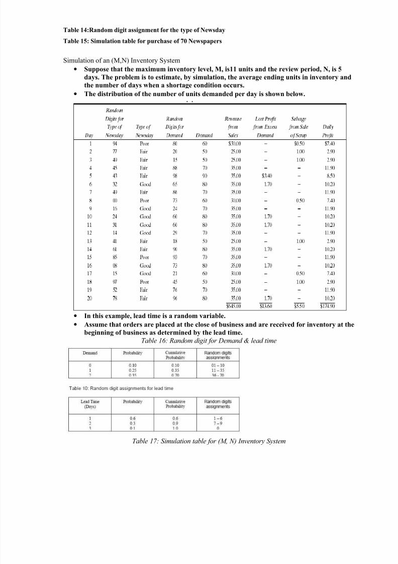
Table 14:Random digit assignment for the type of Newsday

Table 15: Simulation table for purchase of 70 Newspapers

Simulation of an (M,N) Inventory System

• Suppose that the maximum inventory level, M, is11 units and the review period, N, is 5

days. The problem is to estimate, by simulation, the average ending units in inventory and

the number of days when a shortage condition occurs.• The distribution of the number of units demanded per day is shown below.

• In this example, lead time is a random variable.

• Assume that orders are placed at the close of business and are received for inventory at the

beginning of business as determined by the lead time.

Table 16: Random digit for Demand & lead time

Table 17: Simulation table for (M, N) Inventory System



The simulation has been started with the inventory level at 3 units and an order of 8 units

scheduled to arrive in 2 days' time.

• The lead time for this order was 1 day.

• Notice that the beginning inventory on the second day of the third cycle was zero. An order

for 2 units on that day led to a shortage condition.

• The units were backordered on that day and the next day also. On the morning of day 4 of

cycle 3 there was a beginning inventory of 9 units. The 4 units that were backordered and

the 1 unit demanded that day reduced the ending inventory to 4 units.

• Based on five cycles of simulation, the average ending inventory is approximately 3.5 (88 ¸

25) units. On 2 of 25 days a shortage condition existed.

2.3 Other Examples of SimulationA Reliability Problem

Beginning Inventory of

Third day

Ending Inventory of

2 day in first cyclenew order

= +

Beginning Inventory of

Third day

Ending Inventory of

2 day in first cyclenew order

= +



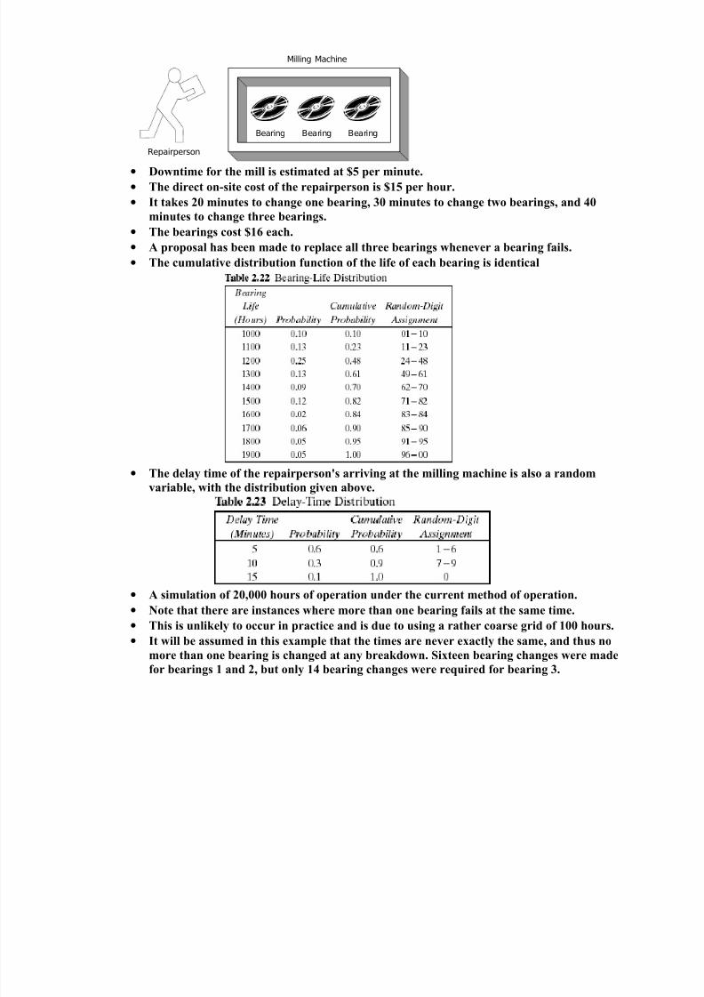
• Downtime for the mill is estimated at $5 per minute.

• The direct on-site cost of the repairperson is $15 per hour.

• It takes 20 minutes to change one bearing, 30 minutes to change two bearings, and 40

minutes to change three bearings.

• The bearings cost $16 each.

• A proposal has been made to replace all three bearings whenever a bearing fails.

• The cumulative distribution function of the life of each bearing is identical

• The delay time of the repairperson's arriving at the milling machine is also a random

variable, with the distribution given above.

• A simulation of 20,000 hours of operation under the current method of operation.

• Note that there are instances where more than one bearing fails at the same time.• This is unlikely to occur in practice and is due to using a rather coarse grid of 100 hours.

• It will be assumed in this example that the times are never exactly the same, and thus no

more than one bearing is changed at any breakdown. Sixteen bearing changes were made

for bearings 1 and 2, but only 14 bearing changes were required for bearing 3.

Repairperson

Milling Machine

Bearing BearingBearing



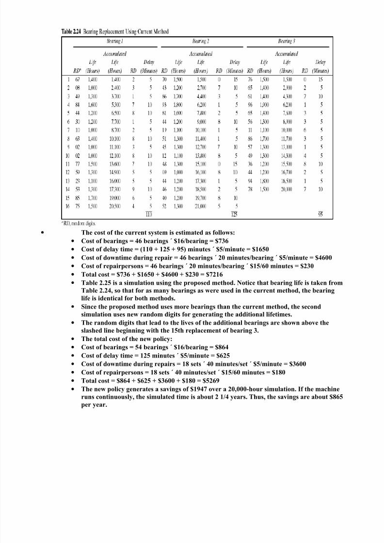
• The cost of the current system is estimated as follows:

• Cost of bearings = 46 bearings ´ $16/bearing = $736

• Cost of delay time = (110 + 125 + 95) minutes ´ $5/minute = $1650• Cost of downtime during repair = 46 bearings ´ 20 minutes/bearing ´ $5/minute = $4600

• Cost of repairpersons = 46 bearings ´ 20 minutes/bearing ´ $15/60 minutes = $230

• Total cost = $736 + $1650 + $4600 + $230 = $7216

• Table 2.25 is a simulation using the proposed method. Notice that bearing life is taken from

Table 2.24, so that for as many bearings as were used in the current method, the bearing

life is identical for both methods.

• Since the proposed method uses more bearings than the current method, the second

simulation uses new random digits for generating the additional lifetimes.

• The random digits that lead to the lives of the additional bearings are shown above the

slashed line beginning with the 15th replacement of bearing 3.• The total cost of the new policy:

• Cost of bearings = 54 bearings ´ $16/bearing = $864

• Cost of delay time = 125 minutes ´ $5/minute = $625

• Cost of downtime during repairs = 18 sets ´ 40 minutes/set ´ $5/minute = $3600

• Cost of repairpersons = 18 sets ´ 40 minutes/set ´ $15/60 minutes = $180

• Total cost = $864 + $625 + $3600 + $180 = $5269

• The new policy generates a savings of $1947 over a 20,000-hour simulation. If the machine

runs continuously, the simulated time is about 2 1/4 years. Thus, the savings are about $865

per year.



Random Normal Numbers

A classic simulation problem is that of a squadron of bombers attempting to destroy anammunition depot shaped as shown below:

• If a bomb lands anywhere on the depot, a hit is scored. Otherwise, the bomb is a miss.

• The aircraft fly in the horizontal direction.

• Ten bombers are in each squadron.• The aiming point is the dot located in the heart of the ammunition dump.

• The point of impact is assumed to be normally distributed around the aiming point with astandard deviation of 600 meters in the horizontal direction and 300 meters in the verticaldirection.



• The problem is to simulate the operation and make statements about the number of bombson target.

• The standardized normal variate, Z, with mean 0 and standard deviation 1, is distributed a

where X is a normal random variable, is the true mean of the distribution of X, and is thestandard deviation of X.

• In this example the aiming point can be considered as (0, 0); that is, the value in thehorizontal direction is 0, and similarly for the value in the vertical direction,

where (X,Y) are the simulated coordinates of the bomb after it has fallen

• The values of Z are random normal numbers.o These can be generated from uniformly distributed random numbers, as discussed

in Chapter 7.o Alternatively, tables of random normal numbers have been generated. A small

sample of random normal numbers is given in Table A.2.o For Excel, use the Random Number Generation tool in the Analysis TookPak Add-In

to generate any number of normal random values in a range of cells.

• The table of random normal numbers is used in the same way as the table of randomnumbers.

• The mnemonic stands for .random normal number to compute the x coordinatcorresponds to above.

• The first random normal number used was –0.84, generating an x coordinate 600(-0.84) =-504.

•The random normal number to generate the y coordinate was 0.66, resulting in a ycoordinate of 198.

• Taken together, (-504, 198) is a miss, for it is off the target.

• The resulting point and that of the third bomber are plotted on Figure 2.8.

• The 10 bombers had 3 hits and 7 misses.

σ

µ −=X

Z µ σ +=Z X σ

µ −=X

Z µ σ +=Z X

X Z X σ =

Y Z Y σ =

X Z X σ =

Y Z Y σ =

600=X

σ 300=Y

σ

iZ X 600= iZ Y 300=

600=X

σ 300=Y

σ

iZ X 600= iZ Y 300=



• Many more runs are needed to assess the potential for destroying the dump.

• This is an example of a Monte Carlo, or static, simulation, since time is not an element of the

solution.

Lead-Time Demand

• Lead-time demand may occur in an inventory system.

•The lead time is the time from placement of an order until the order is received.

• In a realistic situation, lead time is a random variable.

• During the lead time, demands also occur at random. Lead-time demand is thus a randomvariable defined as the sum of the demands over the lead time, or

where i is the time period of the lead time, i = 0, 1, 2, … , Di is the demand during the ith

time period; and T is the lead time.

• The distribution of lead-time demand is determined by simulating many cycles of lead timeand building a histogram based on the results.

• The daily demand is given by the following probability distribution:

• The lead time is a random variable given by the following distribution:

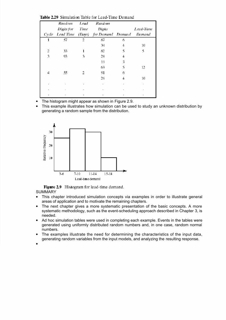
• The incomplete simulation table is shown in Table 2.29.

• The random digits for the first cycle were 57. This generates a lead time of 2 days.

• Thus, two pairs of random digits must be generated for the daily demand.

∑=

T

i iD

0



• The histogram might appear as shown in Figure 2.9.

• This example illustrates how simulation can be used to study an unknown distribution bygenerating a random sample from the distribution.

SUMMARY

• This chapter introduced simulation concepts via examples in order to illustrate generalareas of application and to motivate the remaining chapters.

• The next chapter gives a more systematic presentation of the basic concepts. A moresystematic methodology, such as the event-scheduling approach described in Chapter 3, isneeded.

• Ad hoc simulation tables were used in completing each example. Events in the tables weregenerated using uniformly distributed random numbers and, in one case, random normalnumbers.

• The examples illustrate the need for determining the characteristics of the input data,generating random variables from the input models, and analyzing the resulting response.

•

SMS NOTES 1st UNIT 8th Sem

Documents

Transcript of SMS NOTES 1st UNIT 8th Sem