Smooth Scan: Robust Query Executionwith a Statistics-oblivious Access Operator

Technical Report

Ref: EPFL-REPORT-200188

Renata Borovica-Gajic

Advisor: Anastasia Ailamaki

Data-Intensive Applications and Systems laboratory (DIAS)School of Computer and Communication Sciences

Ecole Polytechnique Federale de Lausanne

renata.borovica@epfl.ch

1

ABSTRACTQuery optimizers depend heavily on statistics representing columndistributions to create efficient query plans. In many cases, though,statistics are outdated or non-existent, and the process of refresh-ing statistics is very expensive, especially for ad-hoc workloads onever bigger data. This results in suboptimal plans that severely hurtperformance. The main problem is that any decision, once madeby the optimizer, is fixed throughout the execution of a query. Inparticular, each logical operator translates into a fixed choice of aphysical operator at run-time.

In this paper, we advocate for continuous adaptation and mor-phing of physical operators throughout their lifetime, by adjust-ing their behavior in accordance with the statistical properties ofthe data. We demonstrate the benefits of the new paradigm by de-signing and implementing an adaptive access path operator calledSmooth Scan, which morphs continuously within the space of tradi-tional index access and full table scan. Smooth Scan behaves sim-ilarly to an index scan for low selectivity; if selectivity increases,however, Smooth Scan progressively morphs its behavior toward asequential scan. As a result, a system with Smooth Scan requiresno access path decisions up front nor does it need accurate statisticsto provide good performance. We implement Smooth Scan in Post-greSQL and, using both synthetic benchmarks as well as TPC-H,we show that it achieves robust performance while at the same timebeing statistics-oblivious.

1. INTRODUCTIONPerils of Query Optimization Complexity. Query execution

performance of database systems depends heavily on query op-timization decisions; deciding which (physical) operators to useand in which order to place them in a plan is of critical impor-tance and can affect response times by several orders of magni-tude [28]. To find the best possible plan, query optimizers typi-cally employ a cost model to estimate performance of viable al-ternatives. In turn, cost models rely on statistics about the data.With the growth in complexity of decision support systems (e.g.templatized queries, UDFs) and the advent of dynamic web appli-cations, however, the optimizer’s grasp of reality becomes increas-ingly loose and it becomes more difficult to produce an optimalplan [19]. For instance, to defy complexity and make up for lackof statistics, commercial database management systems often as-sume uniform data distributions and attribute value independence,which is in reality hardly the case [10]. As a result, database sys-tems are increasingly confronted with suboptimal plans and subparperformance [5, 13, 15, 32, 34, 37].

Motivating Example. To illustrate the severe impact of incom-plete statistics and consequent suboptimal access path choices, weuse a state-of-the-art commercial system, referred to as DBMS-X,and run the TPC-H benchmark [39] (the exact set-up is discussed inSection 6.2). When considering access paths, the optimizer needsaccurate statistics to estimate the tipping point between a full scanand an index scan to make the proper choice. Figure 1 demon-strates the impact of suboptimal index choices after tuning DBMS-

Motivation TPCH (SF10) 2/2

0.1

1

10

100

1000

Q1

Q2

Q3

Q4

Q5

Q6

Q7

Q8

Q9

Q1

0Q

11

Q1

2Q

13

Q1

4Q

16

Q1

8Q

19

Q2

1Q

22

No

rmal

ized

exe

c. t

ime

(lo

g)

TPC-H Query

Tuned

Original

Setting: TPC-H, SF10, DBMS-X, Tuning tool 5GB space

Figure 1: Non-robust Performance due to Optimization Errors in aState-of-the-art Commercial DBMS when running TPC-H.

X for TPC-H; the graph shows normalized execution times overnon-tuned performance. Despite using the official tuning tool ofDBMS-X in the experiment, for several queries performance de-grades significantly after tuning (e.g., up to a factor of 400 forQ12).1 The only change compared to the original plan of Q12 isthe type of access path operator. This decision however prolongedthe execution time from a minute to 11 hours.

Robust Execution. The core of the problem of suboptimal planslies in the fact that even a small estimation error may lead to a dras-tically different result in terms of performance. For instance, onetuple difference in cardinality estimation can swing the decision be-tween an index scan and a full scan, possibly causing a significantperformance drop. Overall, this results in unpredictable perfor-mance thereby affecting the robustness of the system. In addition,the overall behavior is driven by the accuracy of statistics present inthe current server, which aggravates the testing repeatability acrossdifferent servers or even different invocations (since statistics mightchange in between). Stability and predictability, that imply thatsimilar query inputs should have similar execution performance,are major goals for industrial vendors towards respecting servicelevel agreements (SLA) [33]. This is exemplified, nowadays, incloud environments, offering paid-as-a-service functionality gov-erned by SLAs in environments which are much more ad-hoc thantraditional closed systems. In these cases, a system’s ability to ef-ficiently operate in the face of unexpected and especially adverserun-time conditions (e.g., receiving more tuples from an operatorthan estimated) becomes more important than yielding great perfor-mance for one query input while suffering from severe degradationfor another [21]. We define robustness in the context of query pro-cessing as the ability of a system to efficiently cope with unexpectedand adverse conditions, and deliver near-optimal performance forall query inputs.

Past efforts on robustness focus primarily on dealing with theproblem at the optimizer level [5, 11, 12]. Nonetheless, in dynamicenvironments with constantly changing workloads and data char-acteristics, judicious query optimization performed up front couldbring only partial benefits as the environment keeps changing evenafter optimization. Orthogonal approaches on run-time adaptiv-ity [3, 30, 32, 34], although promising, are lacking the flexibilityat the level of access paths.2 Furthermore, since the violation ofthe optimizer’s estimates usually triggers reoptimization, these ap-

1Similar results have been presented in a related study [7].2They are limited either in their scope (by ignoring intra-operatoradaptivity, or by performing binary switching decisions that in-troduce risks and could lead to thrashing) or with respect to per-formance (by duplicating work and/or transforming operators intoblocking ones).

2

proaches remain sensitive to the accuracy of statistics, which com-plicates testing across different environments.

Smooth Scan. We respond to the need for robust execution byintroducing a novel class of access path operators designed withthe goal of providing robust performance for every input regard-less of the severity of cardinality estimation errors. Since the un-derstanding of the data distributions is a continuous process thatdevelops throughout the execution of a query plan and moreoversince one execution strategy might not be optimal over the entiredata set (i.e., we can have sparse and dense regions with respect tothe tuple placement on disk), we need a new class of morphableoperators that continuously and seamlessly adjust their executionstrategy as the understanding of the data evolves. We introduceSmooth Scan, an operator that morphs between an index look-upand a full table scan, achieving near-optimal performance regard-less of the operator’s selectivity and obliviously to the existing datastatistics. Our aim is to provide graceful degradation with respectto the selectivity increase and be as close as possible to the per-formance that could have been achieved if all necessary statisticswere available. In addition, morphing relieves the optimizer fromchoosing an optimal access path a priori, since the execution enginehas the ability to adjust its behavior at run-time as a response to theobserved operator selectivity.

Contributions. Our contributions are as follows:

• We propose a new paradigm of smooth and morphable phys-ical operators that adjust their behavior and transform fromone operator implementation to another according to the sta-tistical properties of the data observed at run-time.

• We design and implement a statistics-oblivious Smooth Scanoperator that morphs between an index access and a full scanas selectivity knowledge evolves at run-time.

• Using both synthetic benchmarks and TPC-H, we show thatSmooth Scan, implemented fully in PostgreSQL, is a viableoption for achieving near-optimal performance throughoutthe entire selectivity interval, by being either competitivewith or outperforming existing access path alternatives.

2. BACKGROUNDIn order to fully understand the advantages and the mechanisms

of the Smooth Scan operator, this section provides a brief back-ground on traditional access path operators.

Full Table Scan is employed when there are no alternative ac-cess paths, or when the selectivity of the access operator is esti-mated to be high (above 1-10% depending on the system parame-ters). The execution engine starts by fetching the first tuple fromthe first page of a table stored in a heap, and continues accessingtuples sequentially inside the page. It then accesses the adjacentpages until it reaches the last page. Figure 2a depicts an exampleof a full scan over a set of pages in the heap; the number placedon the left-hand side of each tuple indicates the order in which itis accessed. Even if the number of qualifying tuples is small, afull table scan is bound to fetch and scan all pages of a table, sincethere is no information on where tuples of interest might be. Onthe positive side, the sequential access pattern employed by the fulltable scan is one to two orders of magnitude faster than the randomaccess pattern of an index scan.

Index Scan. Secondary (non-clustered) indices are built on topof data pages. They are usually B+-trees containing pointers to tu-ples stored in the heap. Figure 2b depicts a B+-tree built on top ofthe same table we used in Figure 2a. The leaves of the tree pointto the heap data pages. A query with a range predicate needs to

Full table scan

Tuple(T)

Table

Heap Page (P)

123456

789

101112

20092010

...

(a) Full Table Scan

Index access

….

...

Root

...1

2

45

67

3 8

9 10

Internal Nodes

Leaf Nodes

(b) Index ScanFigure 2: Access Paths in a DBMS.

traverse the tree once in order to find the pointer to the first tuplethat qualifies, and then it continues following adjacent leaf point-ers until it finds the first tuple that does not qualify. The upsideof this approach, compared to the full scan, is that only tuples thatare needed are actually accessed. The downside is the random ac-cess pattern when following pointers from the leaf page(s) to theheap (shown as lines with arrows). Since the random access pat-tern is much slower than the sequential one, performance degradesquickly if many tuples need to be selected. Moreover, the more tu-ples qualify, the higher the chance that the index scan needs to visitthe same page more than once.

Sort Scan (Bitmap Scan) represents a middle ground betweenthe previous two approaches. Sort Scan still exploits the secondaryindex to obtain the identifiers (TIDs) of all tuples that qualify, butprior to accessing the heap, the qualifying tuple IDs are sorted inan increasing heap page order. In this way, the poor performanceof the random access pattern gets improved by transforming theaccess into a (nearly) sequential pattern, easily detected by diskprefetchers. This strategy, however, has dramatic influence on theexecution model. The index access that traditionally followed thepipeline execution model, now gets transformed into a blockingoperator which can be harmful, especially when the index is usedto provide an interesting ordering [35]. One advantage of B-treeindices comes from the fact that tuples are accessed in the sortedorder of attributes on which the index is built. Sorting of tuple IDsbased on their page placement breaks the natural index orderingthat needs to be restored by introducing a sorting operator above theindex access (or up in the tree). In addition, the blocking operatorso early in the execution plan could stall the rest of the operators; ifthey require a sorted input, their execution can start only after thesecond sort finishes.

3. SMOOTH ACCESS PATHSWe now present the concept of smooth access path operators that

adjust their execution strategy at run-time to fit the data distribu-tions. We first discuss Switch Scan that switches access path strat-egy with a binary decision at run-time. We then introduce SmoothScan that instead of making a single on/off decision, gradually andadaptively shifts its behavior between access path patterns, avoid-ing performance drops.

Switch Scan. The main cause for suboptimal access paths comesfrom a wrong selectivity estimation. One approach to resolve theproblem is to monitor result cardinality during query execution

3

Smooth access

….

...

...

1

2

3

4

5

6

78

9

10

XX X XX

Flattening AccessEntire Page Probe

Morphing region

Figure 3: Smooth Scan Access Pattern.

and switch the access path strategy when we realize that the ini-tial estimation was wrong. Once the actual cardinality exceeds theexpected result cardinality, we can throw away all the work per-formed until that point and restart the execution with a differentaccess path. A more advanced approach reuses the existing inter-mediate results, e.g., by remembering which tuples and pages theprevious access path already visited.

Switching Perils. Switch Scan bounds the worst case execu-tion time as it will never degrade as much as an index scan onlyapproach. However, it is still not a robust approach. The mainproblem with Switch Scan is that it is based on a binary decisionand switches completely when a certain cardinality threshold is vi-olated. This means that even a single extra result tuple can bring adrastically different performance result if we switch access paths.We refer to the effect of a sudden increase in execution time as aperformance cliff. The performance hit together with the uncer-tainty whether the overhead incurred at the time of a change willbe amortized over the remaining query time renders this approachvolatile and non-robust.

Smooth Scan. The core idea behind Smooth Scan is thus togradually transform between two strategies, i.e., a non-clusteredindex look-up and a full table scan, maintaining the advantages ofboth worlds. Our main objective is to provide smooth behavior, i.e.,at no point should an extra tuple in the result cause a performancecliff. Smooth Scan instead morphs its behavior incrementally, andcontinuously, causing only gradual changes as it goes through thedata and its estimation about result cardinality evolves.

3.1 Morphing MechanismDuring a single scan Smooth Scan can be in three modes, while

morphing between an index and full scan. In each mode the oper-ator performs a gradually increasing amount of work as a result ofthe selectivity increase.

Mode 1: Entire Page Probe. To avoid repeated page accessesfrom which the index scan suffers, in this mode Smooth Scan ana-lyzes all records from each heap page it loads to find qualifyingtuples, trading CPU cost for I/O cost reduction. Since the costof an I/O operation translates to an order of million CPU instruc-tions [17], Smooth Scan invests CPU cycles for reading additionaltuples from each page with minimal CPU overhead. Figure 3 de-picts the access pattern of a Smooth Scan in this mode. As in Figure2, the number at the left-hand-side of each tuple indicates the or-der in which the access path touches this tuple. Within each page,Smooth Scan accesses tuples sequentially.

Mode 2: Flattening Access. When the result cardinality grows,Smooth Scan amortizes the random I/O cost by flattening the ran-dom pattern and replacing it with a sequential one. Flattening hap-pens by reading additional adjacent pages from the heap, i.e., foreach page it has to read, Smooth Scan prefetches a few more adja-

cent pages (read sequentially). An example of a morphing regionis depicted in Figure 3.

Mode 2+: Flattening Expansion. Flattening Access Mode is infact an ever expanding mode. When it first enters Flattening Ac-cess Mode, Smooth Scan starts by fetching one extra page for eachpage it needs to access. However, when it notices result selectivityincrease, Smooth Scan progressively increases the number of pagesit prefetches by multiplying it with a factor of 2. The reason is that,as selectivity increases, the I/O increase of fetching more poten-tially unnecessary pages could be masked by the CPU processingcost of the tuples that qualify. In this way, as the result cardinalityincreases more, Smooth Scan keeps expanding, and conceptually itmorphs more aggressively into a full table scan.

3.2 Morphing PoliciesWe now describe how Smooth Scan changes modes.Greedy Policy. Assuming a worst case scenario, Smooth Scan

can perform morphing expansion after each index probe. In thisway, the morphing expansion greedily follows the selectivity in-crease. The upside of this approach is that, due to its fast conver-gence, its worst case performance resembles the performance of afull scan. The downside is that in the case of low selectivity it in-troduces an overhead of reading unnecessary pages that could notbe masked by useful work.

Selectivity Increase Driven Policy. Blindly morphing betweenthe modes may introduce too much overhead if the I/O cost can-not be overlapped with useful work. With this policy, Smooth Scancontinuously monitors selectivity at run-time, and it expands themorphing region when it notices a selectivity increase. In particu-lar, Smooth Scan computes the result selectivity over the last mor-phing region and it increases the morphing region size each timethe local selectivity over the last morphing region (Eq. (1))3 isgreater than the global selectivity over the so far seen pages (Eq.(2)). If selectivity does not increase, Smooth Scan keeps the pre-vious morphing region size. This way, morphing is performed at apace which is purely driven by the data and the query at hand.

sellocal =#Pres region

#Pseen region(1)

selglobal =#Pres

#Pseen(2)

Elastic Policy. When considering large data sets, it is unlikelythat a single execution strategy will be optimal during the wholescan of a big table in a given query; dense and sparse regions withrespect to the tuple placement on disk frequently appear in such acontext due to skewed data distributions. To benefit from the den-sity discrepancy and use skew as an opportunity, Smooth Scan usesthe Elastic Policy to morph two-ways; it increases the morphingsize over a dense region, while it decreases the morphing regionsize when it passes through a sparse region. More precisely, if thelocal selectivity over the last morphing region is higher than theglobal selectivity over all tuples seen so far, then this implies weare in a denser region, hence we double the morphing size. In theopposite case, we decrease the morphing size for the next morphingregion.

3.3 Morphing Triggering PointWe now present Smooth Scan morphing triggers.Optimizer Driven. Smooth Scan can be introduced to the ex-

isting query stack as a reaction to unfavorable conditions, i.e., as arobustness patch. With this strategy, we initiate morphing once the

3The meaning of the parameters can be found in Table 1.

4

result cardinality exceeds the optimizer’s estimate. A cardinalityviolation is an indication that the optimizer’s estimate is inaccurateand that the chosen access path might be suboptimal. After trigger-ing, Smooth Scan can morph with either of the policies describedin Section 3.2.

SLA Driven. Another option is to take action only when in dan-ger of violating a performance threshold, i.e., a service level agree-ment (SLA). For example, let us assume a given time T as an upperbound (SLA) for the operator execution. In this case, Smooth Scancontinuously monitors execution and has a running estimate of theexpected total cost (based on the cost model discussed in Section5). The moment we realize that unless we switch to more conser-vative behavior we will not be able to guarantee the SLA targetperformance, we trigger morphing with Smooth Scan.

Eager Approach. An alternative approach, which we favor, is tocompletely replace access paths with Smooth Scan. With this strat-egy, we eagerly start with Smooth Scan immediately as of the firsttuple. In this way, we guarantee that the total number of page ac-cesses will be equal to the total number of heap pages in the worstcase. Moreover, with this strategy there is no need to record tuplesproduced before morphing has started (to prevent result duplica-tion), which provides additional benefit and decreases bookkeepinginformation.

In our experiments Eager is the default strategy. We study otherstrategies in detail in the experimental section.

4. INTRODUCING SMOOTH PATHS INTOPOSTGRESQL

In this section, we discuss the design details of smooth accessoperators, and their interaction with the remaining query process-ing stack. We implement our operators, both the Switch Scan andSmooth Scan families in PostgreSQL 9.2.1 DBMS as classical phys-ical operators existing side by side with the traditional access pathoperators. During query execution, the access path choice is re-placed by the choice of Smooth Scan, while the upper layers ofquery plans generated by the optimizer remain intact. Unlike thedynamic reoptimization approaches proposed in [2,3], our proposalrequires minimal changes to the existing database architecture.

Switch Scan could conceptually be considered as an instance ofSmooth Scan with a threshold driven policy (usually the optimizer’sresult cardinality estimate) that abruptly switches to Full Scan afterreaching the threshold. Therefore, we do not discuss it separately;except when performing the experimental evaluation in Section 6.6.

4.1 Design DetailsTo make the Smooth Scan operator work efficiently, several crit-

ical issues need to be addressed.Page ID Cache. To avoid processing the same heap page twice

(since multiple out-of-order leaf pointers of the index can point tothe same page), Smooth Scan keeps track of the pages it has readand records them in a Page ID Cache. The Page ID Cache is abitmap structure with one bit per page. Once a page is processedits bit is set to 1. When traversing the leaf pointers from the index,a bit check precedes a heap page access. Smooth Scan will accessthe heap page only if that page has not been accessed before. Oth-erwise, we skip the leaf pointer (X in Figure 3) and continue theleaf traversal.

Result Cache. If an index is chosen to support an interesting or-der (e.g., in a query with an ORDER BY clause), then the tuple or-der has to be respected. This means that a query plan with SmoothScan cannot consume all tuples the moment it produces them. Toaddress this, the additional qualifying tuples found (i.e., all but the

one specifically pointed to by the given index look-up) are kept inthe Result Cache. The Result Cache is a hash-based data structurethat stores qualifying tuples. In this setting, an index probe is pre-ceded by a hash probe of the Result Cache for each tuple identifierobtained from the leaf pages of the index. If the tuple is found inthe Result Cache it is immediately returned (and could be deleted),otherwise Smooth Scan fetches it from the disk following the cur-rent execution mode. The cache deletion is done in a bulk fashion.We partition the Result cache into a number of smaller caches thatcan be deleted once all tuples from an instance are produced. Bygrouping the caches per key ranges, we can remove all items fromone cache as soon as the key range of the cache is traversed. Thekey range intervals are decided by looking at the root page of theindex, since the root page is a good indicator of the key value distri-butions. Even more precise information on key range distributionscould be obtained by looking at the internal node pages if they arecached in memory (which is to be expected since these pages areusually 1h to 1% of data pages).

Tuple ID Cache. If we switch from the traditional index scanfollowing the Optimizer or SLA Driven strategy, we have to ensurethat the result tuples will not be duplicated. This could happen if aresult tuple is produced by following the traditional index, and lateron we fetch the same page with Smooth Scan. To address this issue,we keep a cache of tuple IDs produced with the traditional access ina bitmap-like structure. Later, while producing tuples with SmoothScan we perform a bit check if the tuple has already been produced.The overhead of the Tuple ID Cache, while relatively low, couldbe avoided if a DBMS maintains a strict (indexkey,T ID) orderingin the secondary index. Then it is sufficient to remember the lasttuple we reached with the traditional index, and ignore tuples with(indexkey,T ID) lower than that last tuple.

Discussion. Both the Page ID and Tuple ID Cache are bitmapstructures, meaning that their size is significantly smaller than thedata set size (they easily fit in memory). To illustrate, their size isusually a couple of MB for hundreds of GB of data. In the TupleID cache, we keep IDs of the tuples produced with the traditionalindex, which is in practice significantly lower than the overall num-ber of tuples. The Result Cache is an auxiliary structure whosesize depends on the access order of tuples, the number of attributesin the payload, and the overall operator selectivity. By groupingcaches per key value, we are able to delete them as soon as theyare not needed. If memory becomes scarce, cache spilling couldbe employed by using overflow files. Caches containing the rangesthe furthest from the current key range are spilled into the overflowfiles that are read upon reaching the range keys belong to.

4.2 Interaction with Query Processing StackSmooth Scan is an access path targeted primarily at preventing

severe degradation due to unexpected selectivity increase. Nonethe-less, its impact goes much beyond.

Simplified Query Optimization. Smooth Scan simplifies thequery optimization process. Effectively, when choosing the accesspath for a select operator the optimizer can always choose a SmoothScan. The Smooth Scan will then make all decisions on-the-flyduring query execution.

Interaction with Other Operators. The output of Smooth Scanis input for other operators in a query plan. Depending on the nextoperator a different variation of Smooth Scan may be used. Forexample, if a Merge Join follows Smooth Scan, then the variantof Smooth Scan with the result caching will be used. If insteadIndex Nested Loops Join (INLJ) is performed, Smooth Scan doesnot have to respect the order of tuples coming from the outer in-put, hence it can produce tuples the moment it finds them. If the

5

Table 1: Cost model parametersParameter DescriptionTS Tuple size (bytes).#T Number of tuples in the relation.PS Page size (bytes).#TP Number of tuples per page.#P Number of pages the relation occupies.KS Size of the indexing key (bytes).sel Selectivity of the query predicate(s) (%).card Number of result tuples.cardmX Number of tuples obtained with Mode X.m0check 0 or 1. Was a traditional index employed first?randcost Cost of a random I/O access (per page).seqcost Cost of a sequential I/O access (per page).cpucost Cost of a CPU operation (per tuple).#Pres Number of pages containing result tuples.#Pres region Number of pages with result in current region.#Pseen Number of pages seen so far.#Pseen region Number of pages in the current region.#randio Number of random accesses.#seqio Number of sequential accesses.

Derived valuesf anout B+-tree fanout.#leaves Number of leaf pages in B+-tree.#leavesres Number of leaf pages with pointers to results.height Height of B+-tree.OPio cost Cost of an operator in terms of I/O.OPcpu cost Cost of an operator in terms of CPU.CR Competitive ratio.

ordering requirement is placed by some of the operators up in thetree, we still employ the first option. If Smooth Scan serves as aninner input (i.e., a parameterized path) to an INLJ join, the resultsper join key could be produced in an arbitrary order. Smooth Scanthus performs morphing per key value which reduces the numberof repeated and random access for that particular key. The latterhelps in the case of multiple matches per key (e.g., in a PK-FKrelationship).

Beyond Traditional Join Operators. We have seen how SmoothScan enables graceful degradation of joins, by reducing randomand repeated I/O accesses either at the table level (when served asan outer input) or per join key value (e.g. when served as an innerinput to INLJ). By employing the same concept of smooth morph-ing and transformation, we could benefit even more at the level ofjoin operators. For instance, by performing caching of additional(qualifying) tuples from the inner input found along the way (i.e.,for each page we fetch, we put the remaining tuples in the cache),INLJ morphs into a variant of Hash Join (HJ) overtime, with the in-dex used only when a tuple is not found in the cache. Similarly, MJmorphs into a symmetric Hash Join [41], frequently used in datastreaming environments due to its pipelining nature and amenabil-ity for operator reordering at run-time.

Ultimately, a morphable join and a morphable access path opera-tor can significantly reduce the complexity and fragility of existingquery optimizers. We, however, leave a discussion on the join op-erators as an avenue of future work, and do not use the proposedjoin optimization here.

5. MODELING SMOOTH ACCESS PATHSTo better grasp the behavior of different access path alternatives,

and to answer the critical questions of which policy and mode we

should use and when, in this section we model the operators ana-lytically. Since Smooth Scan trades CPU for I/O cost reduction, wemodel the cost of the operators both in terms of the number of diskI/O accesses, and their CPU cost. Since one I/O operation maps toan order of million CPU cycles [17], it is expected the overall costto be dominated by the I/O component; nonetheless, we discloseCPU costs for completeness. Moreover, we make a distinction be-tween the cost of a sequential and random access, since the natureof the accesses drives the overall query performance.

#TP = bPS

TSc (3)

#P = d #T#TPe (4)

f anout = b PS

1.2×KSc (5)

#leaves = d #Tf anout

e (6)

height = dlog f anout (#leaves)e+1 (7)card = sel×#T (8)

#leavesres = d cardf anout

e (9)

OPcost = OPio cost +OPcpu cost (10)

Table 1 contains the parameters of the cost model. Formulas calcu-lating the cost of the non-clustered index scan and the full scan arepresented for comparison purposes (similar cost model formulasare found in database text books). We assume indices are imple-mented as B+-trees, with k as the tree fanout. Equations 1-7 arebase formulas used for all access path operators. The final costof every operator is a sum of its I/O and CPU costs. We simplifythe calculations by assuming every page is filled completely(100%)and that heap pages and index pages are of the same size (PS).Lastly, we assume that TS already includes a tuple overhead (usu-ally padding and a tuple header). In Eq. (5), we calculate the fanoutof the B+-tree by adding 20% of space per key for a pointer to alower level. For Eq. (6) and (9), we assume that every tuple storedin a heap page has a pointer to it in a leaf page of the index.

Full Table Scan. The cost of full scan does not depend on thenumber of tuples that qualify for the given predicate(s). Thus, re-gardless of the selectivity of the operator its cost remains constant.As shown in Eq. (11), the I/O cost is equal to the cost to fetchall pages of the relation sequentially. Once we fetch a page, weperform a tuple comparison for all tuples from the page to find theones that qualify. In Eq. (12) (and further on) we assume that eachcomparison invokes one CPU operation.

FSio cost = #P× seqcost (11)FScpu cost = #T × cpucost (12)

Index Scan. To fetch the tuples with the (non-clustered) indexscan, we traverse the tree once to find the first tuple that qualifies(height in Eq. (13)). For the remaining tuples, we continue travers-ing the leaf pages from the index (#leavesres×seqcost ) and use tupleIDs we found to access the heap pages, potentially triggering a ran-dom I/O operation per look-up. While traversing the tree for everyindex page we perform a binary search in order to find a pointer ofinterest to the next level (in Eq. (14)). For each tuple obtained byfollowing the pointers from the leaf we perform a tuple comparison

6

to see whether it qualifies.

ISio cost = (height + card)× randcost

+ #leavesres× seqcost (13)IScpu cost = (height× log2( f anout)+ card)× cpucost (14)

Smooth Scan. We calculate the cost of Smooth Scan for eachmode separately. Overall result cardinality is split between themodes (Eq. (15)). Like the index scan, the cost of the smoothscan access is driven by selectivity. Assuming uniform distribu-tion of the result tuples (worst case scenario), the number of pagescontaining the result is calculated in Eq. (16).

card = cardm0 + cardm1 + cardm2 (15)#Pres = min(card,#P) (16)

Mode 0: Index Scan. If the traditional index is employed priorto morphing, the I/O cost to obtain first cardm0 tuples is identicalto the cost of the index scan for the same number of tuples, hencewe omit the formula. A slight difference is in calculating the CPUcost of the operator in Mode 0 (the multiplier 2 in Eq. (17)), to addtuple IDs to the Tuple ID cache.

SScpu cost m0 = (height× log2( f anout)

+ cardm0×2)× cpucost (17)

Mode 1: Entire Page Probe. We calculate the number of tuplesfor which Mode 1 is going to be employed in Eq. (18) (again worstcase). Every page is assumed to be fetched with a random access(Eq. (19)). Once we obtain a page, we perform a tuple comparisonfor all tuples from the page (the first part of Eq. (20)). Beforefetching the page we check whether the page is already processed,and upon its processing we add it to the Page Cache (the secondpart of Eq. (20)). Finally, if we started with the traditional index foreach tuple we have to perform a check whether the tuple has alreadybeen produced in Mode 0 (the third part Eq. (20)). In the case weneed to support an interesting order, the Result Cache will be usedas a replacement for the Tuple ID cache functionality. In that casewe only mark the tuple ID as a key in the cache, without copyingthe actual tuple as a hash value; the probe match without the actualresult thus signifies that the tuple has already been produced. Thus,the CPU cost remains (roughly) the same in both cases.

#Pm1 = min(cardm1,#P) (18)SSio cost m1 = #Pm1× randcost (19)

SScpu cost m1 = (#Pm1×#TP +#Pm1×2+ #Pm1×#TP×m0check)× cpucost (20)

Mode 2: Flattening Access. We calculate the maximum num-ber of pages to fetch with Mode 2 in Eq. (21). Notice that pagesprocessed in Mode 1 are skipped in Mode 2. The nature of themorphing expansion in Mode 2 of Smooth Scan is described withEq. (22). The solution of the recurrence equation is shown in Eq.(23). In our case, n is the number of times we expand the morphingsize (i.e., the number of times we perform a random I/O access) andf (n) translates to the number of pages to fetch with Mode 2 (#Pm2).We obtain the minimum number of random accesses (jumps) tofetch all pages containing the results from Eq. (25). This num-ber is the best case scenario, when the access pattern is such thatall pages are fetched with the flattening pattern without repeatedaccesses. The worst case scenario number of random accesses isshown in Eq. (26). When selectivity is low, the number of ran-dom I/O accesses could at worst be equal to the number of pagesthat contain the results. Nonetheless, there is an upper bound to it,equal to the logarithm of the number of pages in total.

Since both formulas (25) and (26) converge to the same valueequal to log2(#P+ 1), we use this value in the remainder of thesection. The I/O cost of Mode 2 of Smooth Scan is shown in Eq.(27), and is equal to the cost of the number of jumps with a randomaccess pattern, plus the cost to fetch the remaining number of pageswith a sequential pattern. The CPU cost per page in Mode 2 isidentical to the cost per page in Mode 1 (Eq. (28)).

#Pm2 = min(cardm2,#P−#Pm1) (21)f (i+1) = 2× f (i), i = 0..n (22)

f (0) = 0, f (n) = 2n,n >= 0 (23)

#Pm2 =#randio(m2 min)

∑i=0

2i (24)

#randio(m2 min) = log2 (#Pm2 +1) (25)#randio(m2 max) = min(#Pm2, log2 (#P+1)) (26)

SSio cost m2 = #randio(m2)× randcost

+ (#Pm2−#randio(m2))× seqcost (27)SScpu cost m2 = (#Pm2×#TP +#Pm2×2

+ #Pm2×#TP ∗m0check)× cpucost (28)

Finally, the overall cost is the sum of the operator CPU and I/Ocosts for all employed modes(Eg. (29)).

SSio cost = SSio cost m0 +SSio cost m1 +SSio cost m2

SScpu cost = SScpu cost m0 +SScpu cost m1 +SScpu cost m2

SScost = SSio cost +SScpu cost (29)

The cost model formulas allow us to predict the cost of SmoothScan policies, or to decide when is time to trigger a mode change.For instance, for the SLA driven strategy we know the overall op-erator cost defined by an SLA. Based on that cost and Eq. (29), wecould calculate the cardinality, i.e., the triggering point for SmoothScan calculated for the worst case scenario (selectivity 100%).

5.1 Competitive AnalysisIn this section we perform a competitive analysis comparing the

Smooth Scan operator against optimal decisions throughout the en-tire selectivity interval. We calculate a competitive ratio (CR) asthe maximum ratio between the cost of Smooth Scan and the op-timal solution throughout the entire selectivity interval (Eq. (30)).This number shows the maximum discrepancy from the optimal so-lution. The competitive ratio is a viable metric when consideringrobustness, since it provides bounds on the worst case suboptimal-ity. We first consider Smooth Scan with the Greedy Policy accord-ing to which we increase the morphing size after each index access.Then, we consider the Selectivity Increase (SI) Driven policy thatincreases the morphing region size as a response to the observedlocal selectivity increase. Lastly, we consider the refinement in-troduced with the Elastic Policy according to which the morphingexpansion is performed only in the dense regions of the data set,while we decrease the morphing size in sparse regions.

CR = max(

SScost

OPoptimal

),sel ∈ [0,100%]

= max(

SScost

min(IScost ,FScost ,Oracle)

)(30)

5.1.1 Greedy PolicyThe worst case scenario for the Greedy policy is when everything

we fetch with the flattening access pattern is useless, i.e., it does not

7

0 5000 100000

20

40

60

80Competitive ratio against Index Scan

Com

petit

ive

ratio

Number of pages

CR against Index Scan

(a) CR against Index Scan

0 5000 100001

1.05

1.1

1.15

Competitive ratio against Full Scan

Com

petit

ive

Rat

io

Number of pages

CR against Full Scan

(b) CR against Full Scan

0 100 200 300 400 5000

100

200

300

400

500Index Scan vs FS Optimality

CO

ST

Number of pages

Index ScanFull Scan

(c) Full vs. Index Scan

0 5000 100000

200

400

600

800

Com

petit

ive

Rat

io

Number of pages

CR (Theoretical bound)

(d) CR Theoretical BoundFigure 4: Competitive Analysis of Greedy Policy for Highest Page Miss (Worst Case Scenario)

contain any tuple of the result set. In this case, the number of faultpages (pages which do not contain the result tuples) is maximized.This can happen when the next tuple is always one page ahead ofthe current morphing region. Of course, the order does not haveto be such that the page is strictly ahead, but without the loss ofgenerality we assume this use case scenario, while in order to coverthe most adversarial behavior we consider index accesses betweenmorphing regions to be entirely random.

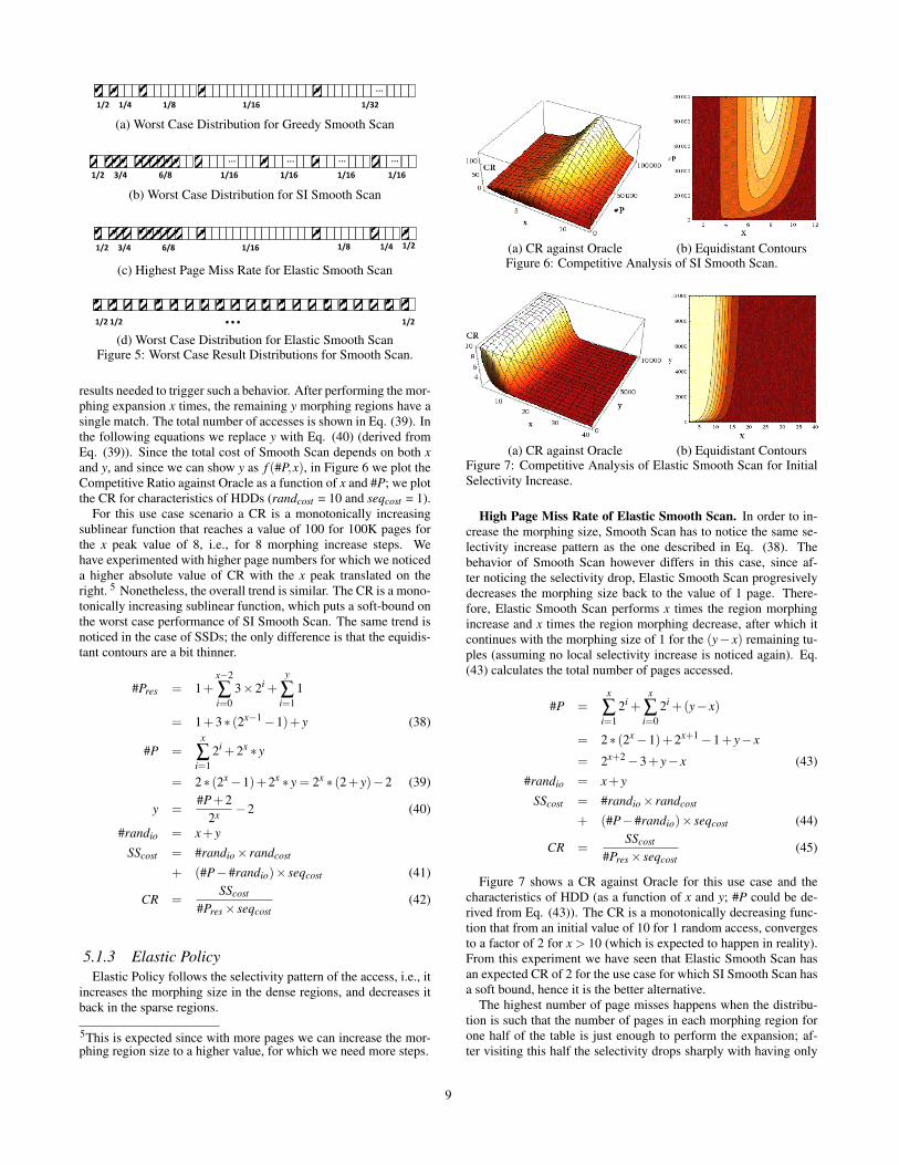
Figure 5a depicts this use case scenario. With striped lines wedenote pages containing results, while empty squares denote faultpages (i.e., page misses). Below each figure describing the resultdistribution pattern, we show the number of page hits (dividend) perthe morphing region size (divisor). The case when Greedy SmoothScan is least effective is when the number of page hits is equal to themaximum number of (random) jumps distributed over the entire ta-ble (depicted in Figure 5a). With the selectivity increase above thisnumber, Smooth Scan’s number of I/O accesses remains constantsince all pages of the table have been accessed, and thus SmoothScan only benefits from further selectivity increase. Therefore, theworst case performance of Smooth Scan is when the cardinality isequal to the number of random jumps (Eq. (31)). Eq. (32) showsthe cost of Smooth Scan for this use case scenario.

card = #randio = log2 (#P+1) (31)SScost = #randio× randcost

+ (#P−#randio)× seqcost (32)

CR =SScost

min(#randio× randcost ,#P× seqcost)(33)

To calculate the competitive ratio we first consider 2 alternatives:A) when Index Scan is the optimal solution, and B) when Full Scanis the optimal solution, both as a function of the table size (thenumber of pages in the table). Then, we compare Smooth Scanagainst a theoretical bound - an Oracle that fetches only pages itneeds with a sequential pattern. This is a pure theoretical boundthat gives the best possible theoretical performance. 4

A) Index Optimal Solution. By assuming Index Scan is theoptimal solution, Eq. (33) becomes:

CR = 1+(#P−#randio)× seqcost

#randio× randcost(34)

In this case, a CR is a monotonically increasing sublinear func-tion that for randcost = 10 and seqcost = 1 (which corresponds tocharacteristics of HDDs) and #P >= 500 starts from a degradationof a factor of 5 and increases to a factor of 72 for #P = 104 (de-picted in Figure 4a).

4The Oracle mimics the behavior of Sort Scan, while ignoring thesorting overhead.

B) Full Scan Optimal Solution. Assuming Full Scan is the op-timal solution, Eq. (33) becomes:

CR = 1+#randio× (randcost − seqcost)

#P× seqcost(35)

This function is a monotonically decreasing function, that for randcost= 10 and seqcost = 1 and #P >= 500 starts from a CR of 1.16(i.e., 16% of overhead when compared to the optimal solution) andreaches 4% for #P = 104 (shown in Figure 4b). This is corroboratedin our experiments, showing that Smooth Scan adds an overhead ofmax 20% when compared to Full Scan. For SSDs (randcost = 2 andseqcost = 1), this value decreases even more (due to lower discrep-ancy between random and sequential IO), starting with an overheadof only 7%.

When is A < B. In Figure 4c we show when each of the alterna-tives is cheaper, for the case when the number of qualifying tuplesis equal the number of random jumps (the worst case scenario de-picted above).

#randio× randcost < #P× seqcost (36)log2 (#P+1)× randcost < #P× seqcost (37)

For p >= 60, randcost = 10 and seqcost = 1 the inequality aboveholds, which means that for the number of pages larger than 60,Index Scan is the optimal solution for this use case scenario, whichunfortunately puts a high soft bound on the worst case performance.

A similar sublinear function (with a higher degradation) is seenwhen comparing Smooth Scan against the optimal Oracle solutionthat fetches only needed pages with a sequential pattern (Figure4d). The CR of Smooth Scan, when compared to Oracle, starts witha factor of 64 for 500 pages and reaches the value 760 for #P= 104.

Discussion. From the competitive analysis we have seen thatGreedy Smooth Scan is not a viable option for low selectivity sinceit can introduce too much overhead due to the high number of faultpages it fetches unnecessarily.

5.1.2 Selectivity Increase Driven PolicySelectivity Increase Driven Policy uses selectivity to drive mor-

phing, i.e., every time a local selectivity increase is noticed, the sizeof the morphing region gets increased. Figure 5b depicts the worstcase distribution for this policy. With this policy, an initial highselectivity can mislead Smooth Scan to keep a high region size (inFigure 5b a morhing size of 16 is kept for the rest of the interval).

In order to increase the morphing size, SI Smooth Scan has tonotice the selectivity increase over the last morphing region biggerthan the selectivity seen so far (calculated in Eq. (1) and Eq. (2) ).A minimal selectivity sequence that will trigger the morphing sizeincrease has to be a sequence 1/2, 3/4, 6/8, 12/16, ..., 3 ∗ 2i−2 /2i ,where the divisor denotes the size of the current morphing regionand the dividend denotes the number of pages containing resultsin this region. Eq. (38) calculates the number of pages containing

8

Competitive analysis

…

1/2 1/4 1/8 1/16 1/32

1/2 3/4 6/8 1/16 1/8 1/4 1/2

…

1/2 1/2 1/2

Worst case pessimistic

Worst page miss rate with Region Density

Worst case Region Density Driven

(a) Worst Case Distribution for Greedy Smooth Scan

…

1/2 1/4 1/8 1/16 1/32

1/2 3/4 6/8 1/16 1/8 1/4 1/2

…

1/2 1/2 1/2

Worst case pessimistic

Worst page miss rate Elastic

Worst case Elastic

1/2 3/4 6/8 1/16 1/16

Worst case Selectivity Increase

…

1/16 1/16

… … …

(b) Worst Case Distribution for SI Smooth Scan

Competitive analysis

…

1/2 1/4 1/8 1/16 1/32

1/2 3/4 6/8 1/16 1/8 1/4 1/2

…

1/2 1/2 1/2

Worst case pessimistic

Worst page miss rate with Region Density

Worst case Region Density Driven(c) Highest Page Miss Rate for Elastic Smooth Scan

Competitive analysis

…

1/2 1/4 1/8 1/16 1/32

1/2 3/4 6/8 1/16 1/8 1/4 1/2

…

1/2 1/2 1/2

Worst case pessimistic

Worst page miss rate with Region Density

Worst case Region Density Driven

(d) Worst Case Distribution for Elastic Smooth ScanFigure 5: Worst Case Result Distributions for Smooth Scan.

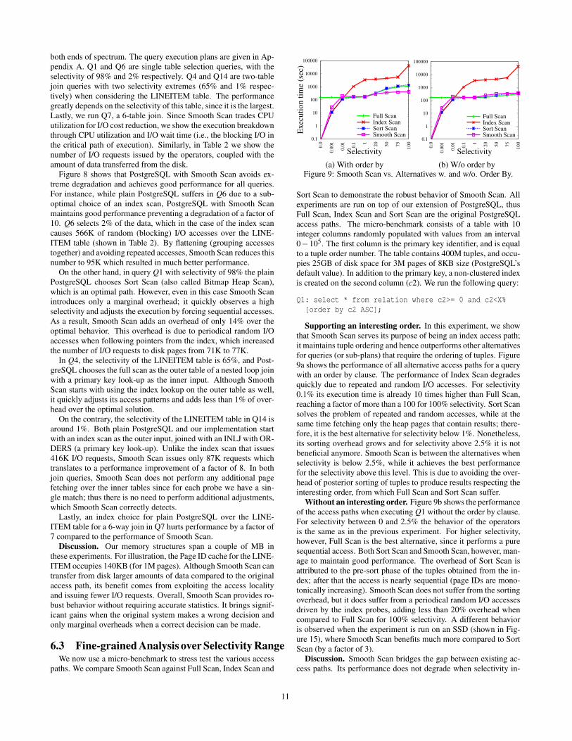
results needed to trigger such a behavior. After performing the mor-phing expansion x times, the remaining y morphing regions have asingle match. The total number of accesses is shown in Eq. (39). Inthe following equations we replace y with Eq. (40) (derived fromEq. (39)). Since the total cost of Smooth Scan depends on both xand y, and since we can show y as f (#P,x), in Figure 6 we plot theCompetitive Ratio against Oracle as a function of x and #P; we plotthe CR for characteristics of HDDs (randcost = 10 and seqcost = 1).

For this use case scenario a CR is a monotonically increasingsublinear function that reaches a value of 100 for 100K pages forthe x peak value of 8, i.e., for 8 morphing increase steps. Wehave experimented with higher page numbers for which we noticeda higher absolute value of CR with the x peak translated on theright. 5 Nonetheless, the overall trend is similar. The CR is a mono-tonically increasing sublinear function, which puts a soft-bound onthe worst case performance of SI Smooth Scan. The same trend isnoticed in the case of SSDs; the only difference is that the equidis-tant contours are a bit thinner.

#Pres = 1+x−2

∑i=0

3×2i +y

∑i=1

1

= 1+3∗ (2x−1−1)+ y (38)

#P =x

∑i=1

2i +2x ∗ y

= 2∗ (2x−1)+2x ∗ y = 2x ∗ (2+ y)−2 (39)

y =#P+2

2x −2 (40)

#randio = x+ y

SScost = #randio× randcost

+ (#P−#randio)× seqcost (41)

CR =SScost

#Pres× seqcost(42)

5.1.3 Elastic PolicyElastic Policy follows the selectivity pattern of the access, i.e., it

increases the morphing size in the dense regions, and decreases itback in the sparse regions.

5This is expected since with more pages we can increase the mor-phing region size to a higher value, for which we need more steps.

(a) CR against Oracle (b) Equidistant ContoursFigure 6: Competitive Analysis of SI Smooth Scan.

(a) CR against Oracle (b) Equidistant ContoursFigure 7: Competitive Analysis of Elastic Smooth Scan for InitialSelectivity Increase.

High Page Miss Rate of Elastic Smooth Scan. In order to in-crease the morphing size, Smooth Scan has to notice the same se-lectivity increase pattern as the one described in Eq. (38). Thebehavior of Smooth Scan however differs in this case, since af-ter noticing the selectivity drop, Elastic Smooth Scan progresivelydecreases the morphing size back to the value of 1 page. There-fore, Elastic Smooth Scan performs x times the region morphingincrease and x times the region morphing decrease, after which itcontinues with the morphing size of 1 for the (y− x) remaining tu-ples (assuming no local selectivity increase is noticed again). Eq.(43) calculates the total number of pages accessed.

#P =x

∑i=1

2i +x

∑i=0

2i +(y− x)

= 2∗ (2x−1)+2x+1−1+ y− x

= 2x+2−3+ y− x (43)#randio = x+ y

SScost = #randio× randcost

+ (#P−#randio)× seqcost (44)

CR =SScost

#Pres× seqcost(45)

Figure 7 shows a CR against Oracle for this use case and thecharacteristics of HDD (as a function of x and y; #P could be de-rived from Eq. (43)). The CR is a monotonically decreasing func-tion that from an initial value of 10 for 1 random access, convergesto a factor of 2 for x > 10 (which is expected to happen in reality).From this experiment we have seen that Elastic Smooth Scan hasan expected CR of 2 for the use case for which SI Smooth Scan hasa soft bound, hence it is the better alternative.

The highest number of page misses happens when the distribu-tion is such that the number of pages in each morphing region forone half of the table is just enough to perform the expansion; af-ter visiting this half the selectivity drops sharply with having only

9

one resulting page per the remaining (shrinking) regions. Figure 5cdepicts such a distribution. We calculate the CR for this scenario.Our analysis shows the theoretical bound of 2.45 for 100 pages thatdecreases to the value of 2.0001 for 3M pages, which corroboratesour previous analysis.

Worst case CR for Elastic Smooth Scan. The previous experi-ment showed the worst scenario with respect to the number of faultpage reads. Nonetheless, this is not the scenario with the worstcase CR. The worst case for Elastic Smooth Scan appears whenthe number of random I/O accesses is maximized. This happenswhen the access is such that every second page has a result match(illustrated in Figure 5d). In this case, Elastic Smooth Scan keepsthe morphing size of 2, since it never detects the local selectivityincrease when compared to the one over so far seen pages. There-fore, Smooth Scan will perform #P/2 random accesses, and thesame amount of sequential accesses (to fetch adjacent pages).

#randio =#P2

(46)

SScost = #randio× randcost

+ (#P−#randio)× seqcost (47)

CR =SScost

min( #P

2 × randcost ,#P× seqcost) (48)

=#P2 × (randcost + seqcost)

min( #P

2 × randcost ,#P× seqcost)

=(randcost + seqcost)

min(randcost ,2× seqcost)

=112

= 5.5

The CR is calculated in Eq. (48). For characteristics of HDDs,with randcost = 10 and seqcost = 1, the competitive ratio reaches thevalue of 5.5 when compared to Full Scan. The same ratio decreasesin the case of SSDs (randcost = 2 and seqcost = 1), reaching a factorof 3. The theoretical bound in this case is 11 for HDDs and 6 forSSDs, and is purely driven by the ratio between the random andsequential access, i.e., it is constant regardless of the table size.

Morphing increase size. A higher morphing increase factorthan 2, leads to a higher Competitive Ratio. For instance, for thisuse case scenario, the morphing increase factor of 10 on HDD givesa competitive ratio of 19. Therefore, we have decided to use a fac-tor of 2 as the morphing increase factor in the rest of the paper.

Discussion. Overall, Elastic Smooth Scan proves to be the mostrobust solution. This policy provides a strong firm bound on thesuboptimality with the maximum theoretical CR of a factor of 11in the case of HDDs and a factor of 6 in the case of SSDs regardlessof the table size. Empirically, we have observed a CR of 2 in ourexperiments, which makes the operator even more appealing.

6. EXPERIMENTAL EVALUATIONWe now present a detailed experimental analysis of Smooth Scan.

We demonstrate that Smooth Scan achieves robust performance ina range of synthetic and real workloads without having accuratestatistics, while existing approaches fail to do so. Furthermore,Smooth Scan proves to be competitive with existing access pathsthroughout the entire selectivity range, making it a viable replace-ment option.

6.1 Experimental SetupSoftware. Our adaptive operators are implemented inside Post-

greSQL 9.2.1 DBMS. To demonstrate the problem of robustness

TPC-H BreakdownSetting: TPC-H, SF10, Indexes proposed by tuning tool

0

200

400

600

800

1000

1200

1400

pSQL pSQL w.Smooth

Scan

pSQL pSQL w.Smooth

Scan

pSQL pSQL w.Smooth

Scan

pSQL pSQL w.Smooth

Scan

pSQL pSQL w.Smooth

Scan

Q1 (98%) Q4 (65%) Q6 (2%) Q7 (30%) Q14 (1%)

Exec

uti

on

tim

e (s

ec) CPU Utilization

I/O Wait time

Figure 8: Improving performance of TPC-H with Smooth Scan.

Table 2: I/O AnalysisQ1 Q4 Q6 Q7 Q14

pSql SS pSql SS pSql SS pSql SS pSql SS#I/OReq.(K) 71 77 225 235 566 95 745 124 416 87

Readdata(GB) 8.9 10.2 10.9 12.1 8.7 8.8 11.6 11.6 6.8 8.9

presented in Section 1 we use a state-of-the-art row-store DBMSwe refer to as DBMS-X.

Benchmarks. We use two sets of benchmarks to showcase algo-rithm characteristics: a) for stress testing we use a micro-benchmark,and b) to understand the behavior of the operators in a realistic set-ting we use the TPC-H benchmark SF 10 [39].

Hardware. All experiments are conducted on servers equippedwith 2 x Intel Xeon X5660 Processors, @2.8 GHz (with L1 32KB,L2 256KB, L3 12MB caches), with 48 GB RAM, and 2 x 300 GB15000 RPM SAS disks (RAID-0 configuration) with an average I/Otransfer rate of 130 MB/s, running Ubuntu 12.04.1. In all experi-ments we report cold runs; we clear database buffer caches as wellas OS file system caches before each query execution.

6.2 TPC-H analysisTPC-H in DBMS-X. In Figure 1 in Section 1, we demonstrated

the severe impact of sub-optimal index choices on the overall TPC-H workload. For this experiment, we used the tuning tool providedas part of DBMS-X, with 5GB of space allowance (1/2 of the dataset size) to propose a set of indices estimated to boost performanceof the TPC-H workload. In queries Q12 and Q19, the presence ofindices favors a nested loop join when the number of qualifying tu-ples in the outer table is significantly underestimated, resulting ina significant increase in random I/O to access tuples from the in-dex (“table look-up”), which in turn results in severe performancedegradation (factors 400 and 20 respectively). In both cases the ac-cess path operator choice is the only change compared to the origi-nal plan, i.e., the join ordering stays the same. Smaller degradationas a result of a suboptimal index choice followed by join reorder-ing occurs in several other queries (Q3, Q18, Q21) resulting in anoverall workload performance degradation by a factor of 22.

Improving performance with Smooth Scan. We now demon-strate a significant benefit that Smooth Scan brings to PostgreSQLcompared to the optimizer’s chosen alternatives when running TPC-H queries. Since PostgreSQL does not have a tuning tool, we createthe set of indices proposed by the commercial system from the pre-vious experiment (on the same workload). Figure 8 shows the re-sults for 5 interesting TPC-H queries6 that cover selectivities from

6These queries represent “choke points” for testing data access lo-cality [6].

10

both ends of spectrum. The query execution plans are given in Ap-pendix A. Q1 and Q6 are single table selection queries, with theselectivity of 98% and 2% respectively. Q4 and Q14 are two-tablejoin queries with two selectivity extremes (65% and 1% respec-tively) when considering the LINEITEM table. The performancegreatly depends on the selectivity of this table, since it is the largest.Lastly, we run Q7, a 6-table join. Since Smooth Scan trades CPUutilization for I/O cost reduction, we show the execution breakdownthrough CPU utilization and I/O wait time (i.e., the blocking I/O inthe critical path of execution). Similarly, in Table 2 we show thenumber of I/O requests issued by the operators, coupled with theamount of data transferred from the disk.

Figure 8 shows that PostgreSQL with Smooth Scan avoids ex-treme degradation and achieves good performance for all queries.For instance, while plain PostgreSQL suffers in Q6 due to a sub-optimal choice of an index scan, PostgreSQL with Smooth Scanmaintains good performance preventing a degradation of a factor of10. Q6 selects 2% of the data, which in the case of the index scancauses 566K of random (blocking) I/O accesses over the LINE-ITEM table (shown in Table 2). By flattening (grouping accessestogether) and avoiding repeated accesses, Smooth Scan reduces thisnumber to 95K which resulted in much better performance.

On the other hand, in query Q1 with selectivity of 98% the plainPostgreSQL chooses Sort Scan (also called Bitmap Heap Scan),which is an optimal path. However, even in this case Smooth Scanintroduces only a marginal overhead; it quickly observes a highselectivity and adjusts the execution by forcing sequential accesses.As a result, Smooth Scan adds an overhead of only 14% over theoptimal behavior. This overhead is due to periodical random I/Oaccesses when following pointers from the index, which increasedthe number of I/O requests to disk pages from 71K to 77K.

In Q4, the selectivity of the LINEITEM table is 65%, and Post-greSQL chooses the full scan as the outer table of a nested loop joinwith a primary key look-up as the inner input. Although SmoothScan starts with using the index lookup on the outer table as well,it quickly adjusts its access patterns and adds less than 1% of over-head over the optimal solution.

On the contrary, the selectivity of the LINEITEM table in Q14 isaround 1%. Both plain PostgreSQL and our implementation startwith an index scan as the outer input, joined with an INLJ with OR-DERS (a primary key look-up). Unlike the index scan that issues416K I/O requests, Smooth Scan issues only 87K requests whichtranslates to a performance improvement of a factor of 8. In bothjoin queries, Smooth Scan does not perform any additional pagefetching over the inner tables since for each probe we have a sin-gle match; thus there is no need to perform additional adjustments,which Smooth Scan correctly detects.

Lastly, an index choice for plain PostgreSQL over the LINE-ITEM table for a 6-way join in Q7 hurts performance by a factor of7 compared to the performance of Smooth Scan.

Discussion. Our memory structures span a couple of MB inthese experiments. For illustration, the Page ID cache for the LINE-ITEM occupies 140KB (for 1M pages). Although Smooth Scan cantransfer from disk larger amounts of data compared to the originalaccess path, its benefit comes from exploiting the access localityand issuing fewer I/O requests. Overall, Smooth Scan provides ro-bust behavior without requiring accurate statistics. It brings signif-icant gains when the original system makes a wrong decision andonly marginal overheads when a correct decision can be made.

6.3 Fine-grained Analysis over Selectivity RangeWe now use a micro-benchmark to stress test the various access

paths. We compare Smooth Scan against Full Scan, Index Scan and

0.1

1

10

100

1000

10000

100000

0.0

0.0

01

0.0

1

0.1 1

20

50

75

10

0

Ex

ecu

tio

n t

ime

(sec

)

Selectivity

Full ScanIndex ScanSort ScanSmooth Scan

(a) With order by

0.1

1

10

100

1000

10000

100000

0.0

0.0

01

0.0

1

0.1 1

20

50

75

100

Selectivity

Full ScanIndex ScanSort ScanSmooth Scan

(b) W/o order byFigure 9: Smooth Scan vs. Alternatives w. and w/o. Order By.

Sort Scan to demonstrate the robust behavior of Smooth Scan. Allexperiments are run on top of our extension of PostgreSQL, thusFull Scan, Index Scan and Sort Scan are the original PostgreSQLaccess paths. The micro-benchmark consists of a table with 10integer columns randomly populated with values from an interval0−105. The first column is the primary key identifier, and is equalto a tuple order number. The table contains 400M tuples, and occu-pies 25GB of disk space for 3M pages of 8KB size (PostgreSQL’sdefault value). In addition to the primary key, a non-clustered indexis created on the second column (c2). We run the following query:

Q1: select * from relation where c2>= 0 and c2<X%[order by c2 ASC];

Supporting an interesting order. In this experiment, we showthat Smooth Scan serves its purpose of being an index access path;it maintains tuple ordering and hence outperforms other alternativesfor queries (or sub-plans) that require the ordering of tuples. Figure9a shows the performance of all alternative access paths for a querywith an order by clause. The performance of Index Scan degradesquickly due to repeated and random I/O accesses. For selectivity0.1% its execution time is already 10 times higher than Full Scan,reaching a factor of more than a 100 for 100% selectivity. Sort Scansolves the problem of repeated and random accesses, while at thesame time fetching only the heap pages that contain results; there-fore, it is the best alternative for selectivity below 1%. Nonetheless,its sorting overhead grows and for selectivity above 2.5% it is notbeneficial anymore. Smooth Scan is between the alternatives whenselectivity is below 2.5%, while it achieves the best performancefor the selectivity above this level. This is due to avoiding the over-head of posterior sorting of tuples to produce results respecting theinteresting order, from which Full Scan and Sort Scan suffer.

Without an interesting order. Figure 9b shows the performanceof the access paths when executing Q1 without the order by clause.For selectivity between 0 and 2.5% the behavior of the operatorsis the same as in the previous experiment. For higher selectivity,however, Full Scan is the best alternative, since it performs a puresequential access. Both Sort Scan and Smooth Scan, however, man-age to maintain good performance. The overhead of Sort Scan isattributed to the pre-sort phase of the tuples obtained from the in-dex; after that the access is nearly sequential (page IDs are mono-tonically increasing). Smooth Scan does not suffer from the sortingoverhead, but it does suffer from a periodical random I/O accessesdriven by the index probes, adding less than 20% overhead whencompared to Full Scan for 100% selectivity. A different behavioris observed when the experiment is run on an SSD (shown in Fig-ure 15), where Smooth Scan benefits much more compared to SortScan (by a factor of 3).

Discussion. Smooth Scan bridges the gap between existing ac-cess paths. Its performance does not degrade when selectivity in-

11

0.01

0.1

1

10

100

1000

10000

100000

0.0

0.0

01

0.0

1

0.1 1 5

20

50

75

100

Exec

uti

on t

ime

(sec

)

Selectivity

Full Scan

Index Scan

Smooth Scan(Entire Page Probe)

Smooth Scan(Flattening Access)

Figure 10: Sensitivity Analysis of Smooth Scan Modes.

creases, like in the case of Index Scan. This is particularly impor-tant in real-life scenarios where a degradation in Index Scan causesperformance drops of several orders of magnitude [19]. At the sametime, Smooth Scan does not pay the cost of Full Scan to select just afew tuples, which is important for point queries for which Full Scanis not practical. When the order is not imposed the absolute perfor-mance of Smooth Scan is comparable to that of Sort Scan; nonethe-less, the benefit of Smooth Scan becomes visible when consideringits placement in the query plan. Unlike Sort Scan, Smooth Scan ad-heres to the pipelining model, which is important since the accesspath operators are executed first and can stall the rest of the stack.When selectivity is below 0.01%, Smooth Scan’s Competitive Ra-tio reaches a factor of 2 over the optimal solution. To put absolutenumbers in perspective, in our experiment a maximal overhead of60 seconds is paid to prevent a worst case performance degradationof 11 hours. In decision support systems that are characterized bylong running queries, this overhead is likely to be tolerable as a ro-bustness guarantee for the prevention of severe performance dropsthat frequently happen due to data correlations and skew.

6.4 Sensitivity analysis of Smooth ScanWe now study the parameters that affect the performance of Smooth

Scan such as the impact of its morphing modes, policies, and strate-gies. We show the bookkeeping overhead and study the SmoothScan effect on HDDs versus SSDs. For all experiments in this sec-tion, unless stated otherwise, we use Q1 from the micro-benchmarkwithout an order by clause.

Impact of the Entire Page Probe Mode. The pointer chasing ofnon-clustered indices when performing a tuple look-up in generalhurts performance when the selectivity increases. Figure 10 depictsthe improvement that Smooth Scan achieves by removing repeatedaccesses when executing query Q1 from the micro-benchmark. Thecurve of Smooth Scan denoted as the Entire Page Probe morphsonly until Mode 1. Smooth Scan improves by a factor of 10 whencompared to Index Scan for selectivity 100%. The performanceof Smooth Scan degrades with selectivity increase up to 1%; thisis the point where approximately all pages have been read. With120 tuples per page (64-byte tuples in 8KB pages) and uniformdistribution, we expect one tuple from each page to qualify. Afterthat point the execution time stays nearly flat with the increase of20% for 100% selectivity, showing that the overhead of readingthe remaining tuples from a page is dominated by the time neededto fetch a page from disk. The execution time of Smooth Scanwhen morphing only up to Mode 1, is however still significantlyhigher (a factor of 14) compared to Full Scan for 100% selectivity.This is due to the discrepancy between random and sequential pageaccesses; the former being an order of magnitude slower in the caseof HDD.

0

100

200

300

400

500

600

0.0

0.0

01

0.0

02

0.0

03

0.0

04

0.0

05

0.0

06

0.0

07

0.0

08

0.0

09

0.0

1 510

20

30

40

50

75

100

Ex

ecu

tio

n t

ime

(sec

)

Selectivity

GreedySelectivity IncreaseElastic

(a) Morphing Policies

0

100

200

300

400

500

600

0.0

0.0

01

0.0

02

0.0

03

0.0

04

0.0

05

0.0

06

0.0

07

0.0

08

0.0

09

0.0

1 510

20

30

40

50

75

100

Selectivity

SLA Bound

EagerOptimizer DrivenSLA Driven

(b) Triggering PointsFigure 11: Impact of Policy and Trigger Choices.

Impact of the Flattening Access Mode. To alleviate the ran-dom access problem, Smooth Scan employs Mode 2+ (shown inFigure 10 as the Flattening Access curve). By fetching adjacentpages Smooth Scan amortizes access costs at the expense of extraCPU cost to go through all the fetched data. We perform a sen-sitivity analysis on the maximum number of adjacent pages up towhich we perform the morphing expansion. Our experiments showthat 2K pages are optimal (translates to a block size of 16MB);thus we keep this value as the maximum region size for the rest ofthe experiments. Smooth Scan with Flattening Access is not onlymuch better than Index Scan (by a factor of 115) but also nearly ap-proaches the behavior of Full Scan; in the worst case of selectivity100% Smooth Scan is only 20% slower than Full Scan.

Impact of Policy Choices. We plot the impact of policy choicesin Figure 11a. The Greedy policy morphs with each index probe,and hence converges to the full scan faster than other policies. Forlower selectivity the Selectivity Increase and Elastic policies intro-duce less overhead compared to the Greedy since they fetch feweradjacent pages, i.e., more pages need to be seen for the morph-ing size to increase. This particularly holds for the Elastic policythat adjusts the morphing size depending on the selectivity of thefetched regions. Since it is the most adaptive to the changes in theoperator selectivity, we favor it in the rest of the experiments.

Impact of Trigger Choices. In Figure 11b, we plot the impactof triggering strategy choices. The Eager strategy starts immedi-ately with Smooth Scan; in this case we plot the Elastic SmoothScan. The Optimizer Driven strategy starts with the traditional in-dex and changes to Smooth Scan after 15K tuples (the optimizer’sestimated cardinality), causing the increase in the execution timefor selectivity 0.005%. After the shift to Smooth Scan, for thisexperiment we continue with the Selectivity Increase Driven pol-icy. The overhead of the Optimizer Driven strategy increases forhigher selectivity compared to the Eager strategy and is attributedto a tuple check for each tuple produced with Smooth Scan, andto additional repeated accesses of the same pages accessed beforethe Smooth Scan behavior is triggered. On the other hand the ini-tial execution time is lower compared to the Eager strategy due tofewer page accesses. Similar behavior is observed with the SLAdriven triggering strategy, with a sharper cliff for point 0.009%,since with this strategy we switch immediately to Greedy. For thisexperiment we have set an upper performance bound equal to theperformance of 2 full scans as the SLA constraint; the calculatedbound is shown as the orange dotted line in Figure 11b. Accordingto the model the morphing triggering point is 32K tuples, whichguarantees the execution time just slightly below the SLA boundfor 100% selectivity.

Overall, the Eager strategy strikes a balance in terms of overallperformance. However, if we are in an environment where respect-

12

0

100

200

300

400

500

600

700

Full Scan

Index Scan

SI Smooth

Elastic Smooth

Ex

ecu

tio

n t

ime (

sec)

Access Path Choice

(a) Execution Time (1% sel.)

0.1

1

10

100

Full Scan

Index Scan

SI Smooth

Elastic Smooth

Nu

mb

er o

f R

ead

Pag

es (

M)

Access Path Choice

(b) Number of Read PagesFigure 12: Handling Skew.

ing SLA is the main priority, or Smooth Scan serves as a means offixing sub-optimal decisions then an SLA or Optimizer strategy areviable alternatives; we easily turn a strategy knob depending on theapplications requirements.

Adjusting to Skew Distribution. Smooth Scan has demon-strated the ability to prevent execution time blow-up due to selec-tivity increase. Many modern applications, however, exhibit non-uniform data distributions (stock markets, internet networks, etc.).For these applications one execution strategy is not likely to opti-mally serve the entire table. We show that Smooth Scan can adaptwell to skewed distribution of values across pages. We use theElastic policy and compare it against the Selectivity Increase (SI)policy.

We use a table with 1.5B tuples, 10 integer columns (randomvalues from [0-105]) that occupy 100GB, and create a secondaryindex on the second column (c2). First 15M tuples have c2 = 0;afterwards another 0.001% of random tuples have value 0. The re-sult selectivity is slightly above 1%, with most of the tuples comingfrom the pages placed at the beginning of the relation heap, i.e. weread all tuples where c2 = 0.

Figure 12a plots the execution time of Index Scan, Full Scan, SIand Elastic Smooth Scan; Figure 12b plots the number of distinctpages fetched to answer the query. From Figure 12b we see thatSI Smooth Scan fetches 56 times more pages than Elastic SmoothScan, and it is 5 times slower. The large number of pages is dueto the initial skew; SI Smooth Scan notices the high selectivity in-crease at the beginning, and in order to reduce the potential degra-dation it continues fetching big chunks of sequentially placed page,ultimately fetching 8.8M out of 12.5M pages. On the contrary, af-ter the dense region, Elastic Smooth Scan decreases the morphingstep, quickly converging back to the access of a single page perprobe, ultimately ending up with only 150K pages fetched (IndexScan fetches 140K pages; the severe impact of repeated and ran-dom I/O is not seen for Index Scan, since the index key followsthe page placement on disk). Elastic Smooth Scan, thus, continuesproviding near-optimal performance, despite the significant initialskew. This is particularly important for long-running queries overbig data, where data distribution tends to be non-uniform [30]. Ap-proaches that employ one execution strategy, or run multiple alter-natives shortly and kill all but the winning one are likely to makea mistake and not be able to benefit from this density discrepancy;Elastic Smooth Scan, however, adjusts its behavior to fit the datadistribution.

Auxiliary Data Structures. To avoid repeated page accesses,Smooth Scan in PostgreSQL uses the data structures described inSection 4.1. We now show the bookkeeping overhead of thesestructures and their hit rate, demonstrated on Q1 from the micro-benchmark with an ORDER BY clause.

0

5

10

15

20

0.0

0.0

01

0.0

1

0.1 1

20

50

75

100

0

20

40

60

80

100

120

Cac

he

Ov

erh

ead

(%

)

Cac

he

Hit

Rat

e (%

)

Selectivity

Cache OverheadCache Hit Rate

(a) Result Cache Analysis

0

20

40

60

80

100

120

0.0

01

0.1 1

2.5 20

50

75

10

0

Morp

hin

g A

ccura

cy(%

)

Selectivity

Accuracy

(b) Morphing AccuracyFigure 13: Analysis of Auxiliary Data Structures.

Figure 13a shows that Result Cache adds a maximal overhead of14% when storing all result matches in the cache (shown as bluebars). At the same, the Result Cache Hit Rate (calculated as theratio between the number of tuple requests served from the cacheand the total number of tuple requests) reaches 100% for 1% se-lectivity. Figure 13b shows that the morphing accuracy (calculatedas the ratio between the number of pages containing result matchesand the total number of checked pages with Smooth Scan morph-ing) gets improved after 1%, reaching 100% for 2.5% selectivity.The overhead of page ID checks remains significantly below 1% inall our experiments, hence we do not show it separately.

Cost Model Analysis. In this experiment we show that the esti-mates of the analytical model we derived are corroborated with theactually measured performance. Figure 14a and Figure 14b showthe cost behavior of Full Scan, Index Scan, and Smooth Scan basedon the analytical cost model, as a function of selectivity. The y-axisshows the cost (unit 1 corresponds to one sequential I/O). We modelthe costs for a table with 400M tuples from the micro-benchmarks.For the page size we take the value of 8KB; for the tuple size weassume 64 bytes (40 bytes of data plus the overhead for the tupleheader), and for the key size we use 16 bytes. We assume uniformdistribution of result tuples, and approximate the number of randomI/O accesses for Mode 2 with log2(#P+1). Finally, for seqcost weuse 1, for randcost we use 10, and for cpucost we use 1/1M. Weseparately show the behavior of the operators when selectivity isbetween 0 and 1%, since for the increasing selectivity both FullScan and Smooth Scan converge to the same value.

The model suggests that for lower selectivity Smooth Scan be-haves like Index Scan, while for higher selectivity it converges tothe performance of Full Scan. This is corroborated in our exper-iments presented in Figure 14c and Figure 14d; they depict thereal execution times using the actual data that the model assumed.In both graphs Smooth Scan converges to Full Scan as predicted.The only discrepancy from the model we observe is that SmoothScan converges faster to Full Scan than estimated. This effect ispartly due to the disk controller behavior, grouping many sequen-tial I/O requests from the disk controller queue into one in the caseof Full Scan, which puts the performance bar of Full Scan a bitlower than expected. Similar behavior is not observed in the caseof Smooth Scan that issues requests for sequential sub-arrays withrandom jumps in between. Although the same grouping of sequen-tial sub-arrays could happen and equally improve performance, thedisk controller did not possess logic to do so.

6.5 Smooth Scan on SSDGiven the different access costs of solid state disks (SSD), better

random access performance, and the forecasts of their potential re-placement of HDD [23], we now stress test Smooth Scan on SSD.We use a solid state disk OCZ Deneva 2C Series SATA 3.0 with

13

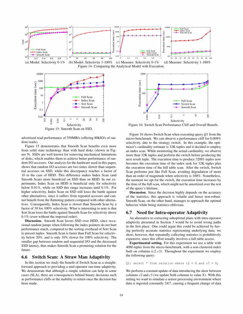
0 0.2 0.4 0.6 0.8 110

0

102

104

106

108

Cos

t

Selectivity

Full ScanIndex ScanSmooth Scan

(a) Model: Selectivity 0-1%20 40 60 80 100

106

107

108

109

1010

Cos

t

Selectivity(b) Model: Selectivity 1-100%

0.01

0.1

1

10

100

1000

10000

0 0.2 0.4 0.6 0.8 1

Ex

ecu

tio

n t

ime

(sec

)

Selectivity

Full ScanIndex ScanSmooth Scan

(c) Measure: Selectivity 0-1%

100

1000

10000

100000

10 20 30 40 50 60 70 80 90 100

Ex

ecu

tio

n t

ime

(sec

)

Selectivity

Full ScanIndex ScanSmooth Scan

(d) Measure: Selectivity 1-100%Figure 14: Comparing the Analytical Model with Execution.

0.01

0.1

1

10

100

1000

10000

0.0

0.0

01

0.0

1

0.1 1 5

20

50

75

100

Exec

uti

on t

ime

(sec

)

Selectivity

Full Scan

Index Scan

Sort Scan

Smooth Scan

Figure 15: Smooth Scan on SSD.

advertised read performance of 550MB/s (offering 80kIO/s of ran-dom reads).

Figure 15 demonstrates that Smooth Scan benefits even morefrom solid state technology than with hard disks (shown in Fig-ure 9). SSDs are well known for removing mechanical limitationsof disks, which enables them to achieve better performance of ran-dom I/O accesses. Our analysis for the hardware used in this paper,shows that random I/O accesses are two times slower than sequen-tial accesses on SSD, while this discrepancy reaches a factor of10 in the case of HDD. This difference makes Index Scan (andSmooth Scan) more beneficial on SSD than on HDD. In our ex-periments, Index Scan on HDD is beneficial only for selectivitybelow 0.01%, while on SSD this range increases until 0.1%. Forhigher selectivity, Index Scan on SSD still loses the battle againstother alternatives, since it suffers from repeated accesses and can-not benefit from the flattening pattern compared with other alterna-tives. Consequently, Index Scan is slower than Smooth Scan by afactor of 30 for 100% selectivity. What is interesting to note is thatSort Scan loses the battle against Smooth Scan for selectivity above0.1% (even without the imposed order).

Discussion. Smooth Scan favors SSD over HDD, since occa-sional random jumps when following the index pointers do not hurtperformance much, compared to the sorting overhead of Sort Scanto presort tuples. Smooth Scan is faster than Full Scan for selectiv-ity below 20%, and is only 10% slower for 100% selectivity. Thesmaller gap between random and sequential I/O and the decreasedSSD latency, thus makes Smooth Scan a promising solution for thefuture.

6.6 Switch Scan: A Straw Man AdaptivityIn this section we study the benefit of Switch Scan as a straight-

forward approach to providing a mid-operator run-time adaptivity.We demonstrate that although a simple solution can help in somecases (SLA), there are consequences behind binary decisions suchas performance cliffs or the inability to return once the decision hasbeen made.

10

100

1000

0.0

01

0.0

1

0.1 1

10

10

0

Exec

uti

on t

ime

(sec

)

Selectivity

Full Scan

Switch Scan

Smooth Scan

Figure 16: Switch Scan Performance Cliff and Overall Benefit.

Figure 16 shows Switch Scan when executing query Q1 from themicro-benchmark. We can observe a performance cliff for 0.009%selectivity, due to the strategy switch. In this example, the opti-mizer’s cardinality estimate is 32K tuples and it decided to employan index scan. While monitoring the actual cardinality, we observemore than 32K tuples and perform the switch before producing thenext result tuple. The execution time to produce 32001 tuples nowbecomes the execution time of the index seek for 32K tuples plusthe execution time of the full table scan. After the switch, SwitchScan performs just like Full Scan, avoiding degradation of morethan an order of magnitude when selectivity is 100%. Nonetheless,the moment we opt for the switch, the execution time increases bythe time of the full scan, which might not be amortized over the restof the query’s lifetime.

Discussion. Since the decision highly depends on the accuracyof the statistics, this approach is volatile and hence non-robust.Smooth Scan, on the other hand, manages to approach the optimalbehavior while being statistics-oblivious.

6.7 Need for Intra-operator AdaptivityAn alternative to correcting suboptimal plans with intra-operator

adaptivity presented in Section 3 would be to avoid wrong pathsin the first place. One could argue this could be achieved by hav-ing perfectly accurate statistics representing underlying data; weshow, however, that repeatedly collecting statistics is prohibitivelyexpensive, since this effort usually involves a full table access.

Experimental setting. For this experiment we use a table with40M tuples from the micro-benchmark, with a non-clustered indexbuilt on columns (c2,c3). Throughout the experiment we employthe following query:

Q2: select * from relation where c2 = X and c3 = X;

We perform a constant update of data introducing the skew betweencolumns c2 and c3 (we update both columns to value X). With thissetting we want to simulate a sensor processing environment wheredata is ingested constantly 24/7, causing a frequent change of data

14

All together

0

50

100

150

200

0 20 40 60 80 100

Exec

uti

on

tim

e (s

ec)

Result selectivity (%)

Full ScanIndex ScanOptimizer decisionAvg. statistics collection

0

50

100

150

200

0 20 40 60 80 100

Result selectivity (%)

0

50

100

150

200

0 20 40 60 80 100

Result selectivity (%)

(a) Basic statistics

All together

0

50

100

150

200

0 20 40 60 80 100

Exec

uti

on

tim

e (s

ec)

Result selectivity (%)

Full ScanIndex ScanOptimizer decisionAvg. statistics collection

0

50

100

150

200

0 20 40 60 80 100

Result selectivity (%)

0

50

100

150

200

0 20 40 60 80 100

Result selectivity (%)

(b) Single column

All together

0

50

100

150

200

0 20 40 60 80 100

Exec

uti

on

tim

e (s

ec)

Result selectivity (%)

Full ScanIndex ScanOptimizer decisionAvg. statistics collection

0

50

100

150

200

0 20 40 60 80 100

Result selectivity (%)

0

50

100

150

200

0 20 40 60 80 100

Result selectivity (%)

(c) Column groupFigure 17: Statistics Collection Alternatives in DBMS-X.

statistics. Completely accurate statistics representing underlyingdata are rarely present in such a system.

Figure 17 shows the statistics collection times on the table, com-paring them against the execution time of query Q2 run on DBMS-X7. The three graphs demonstrate the three levels of database statis-tics, namely: a) base statistics (the table size, tuple size, number oftuples, etc.); b) single column distribution statistics (histograms oneach column separately); c) joint-data distributions (a histogram onthe group of columns from the query (c2, c3)).

Statistics types analysis. Despite being the cheapest alternative,the basic statistics could still lead to the choice of suboptimal plansas shown in Figure 17a since they cannot accurately detect neitherskew nor the presence of column correlations. On the other hand,one could observe that obtaining histograms on all columns intro-duces a higher cost as shown in Figure 17b. Having histograms onall columns could solve the problem of suboptimal decisions in thecase of skewed data. Nevertheless, it will still not detect the correla-tion between different columns (notice the sub-optimal decision forselectivity 40% in Figure 17b). Therefore, whenever a query con-tains multiple filtering predicates over different columns, joint-datadistributions are required. Figure 17c shows the statistics collectiontime on the group of two columns from the query. Performing thiscollection once could be tolerated. Calculating all possible jointdistributions for the workload consisting of many queries, how-ever, is an unattainable goal, especially since applications todayhave hundreds of columns in each table [37].

Incomplete statistics hurt performance. Query Q2 is a simplequery that showcases the problem with existing DBMS. Assumingno accurate statistics exist on the table, the optimizer would fall intoa trap of using the non-clustered index regardless of the actual re-sult cardinality. This is happening because the uniformity assump-tion assumes the selectivity of each predicate to be 10−5 (1/100K),while the independence further assumes the overall selectivity to be10−10 ( 10−5 ∗10−5) [10]. Therefore, the optimizer would alwaysopt for the non-clustered index look-up, severely hurting perfor-mance in the case of higher selectivity.

7. RELATED WORKSmooth Scan draws inspiration from a large body of work on

adaptive and robust query processing. We briefly discuss the workmore related to our approach, while for a detailed summary theinterested reader may refer to [13].

Statistics Collection. Since the quality of plans directly de-pends on the accuracy of data statistics, a plethora of work hasstudied techniques to improve the statistics accuracy in DBMS.

7We have measured statistics collection time on a commercial sys-tem, since this system supports a wider spectrum of possibilitiesthan PostgreSQL.

Modern approaches employ the idea of monitoring execution toexploit this information in future query compilations [1, 8, 37]. Indynamically changing environments, however, statistical informa-tion rarely stays unchanged between executions; consider data in-gest different devices produce (e.g. smart meters [25], data fromFacebook, etc.) for instance. Orthogonal techniques focused onmodeling the uncertainty about the estimates durign query opti-mization [4, 5]. Overall, considering the two-dimensional changein the workload characteristics (frequent data ingest, and ad-hocqueries) in modern applications, and the high price of having up-to-date statistics for all cases in the exponential search space [8,9],the risk of having incomplete or stale statistics still remains high.

Single-plan Adaptive Approaches. From the early prototypesto most modern database systems, query optimizers determine asingle best execution plan for a given query [35]. To cope with envi-ronment changes in such systems, some of the early work on adap-tive query processing employed reoptimization techniques in themiddle of query execution [30, 32, 34]. Since this re-optimizationstep can introduce overheads in query execution, an alternative tech-nique proposed in the literature is to choose a set of plans at com-pile time and then opt for a specific plan based on the actual valuesof parameters at run-time [22, 29]. A middle ground between re-optimization and dynamic evaluation is proposed in [5, 15], wherea subset of more robust plans is chosen for given cardinality bound-aries. Regardless of the strategy when to adjust behavior, reopti-mization approaches suffer from similar binary decisions that wehave seen with Switch Scan; once reoptimization is employed, thestrategy switch will almost certainly trigger a performance cliff.

Multi-plan Adaptive Approaches. Some of the early techniqueswith multi-plan approaches employed competition to decide be-tween alternative plans [2, 24]. Essentially, multiple access pathsfor a given table are executed simultaneously for a short time andthe one that wins is used for the rest of the query plan. In con-trast, Smooth Scan does not perform any work that is thrown awaylater (while all the work done for every access method except thewinning one is discarded in the approach of competing plans).

Adaptive and Robust Operators. With workloads being lesssteady and predictable, coarse-grained index tuning techniques arebecoming less useful with the optimal physical design being a mov-ing target. In such environments, adaptive indexing techniquesemerged, with index tuning being a continuous effort instead of aone time procedure. Partial indexing [36,38,42] broke the paradigmof building indices on a full data set, by partitioning data into in-teresting and uninteresting tuples, while indexing only the former.Similarly, but more adaptively using the workload as a driving force,database cracking and adaptive merging techniques [20,26,27] lowerthe creation cost of indices and distribute it over time by piggy-backing on queries to refine indices. Lastly, SMIX indices are in-troduced as a way to combine index accesses with full table scans,by building covered values trees(CVT) on tuples of interest [40].Despite bringing adaptivity in index tuning, none of the techniquesaddresses the index accesses from the aspect of query processing,and hence stayed susceptible to the optimizer’s mistakes. The clos-est to our motivation of achieving robustness in query processing isG-join [18], an operator that combines strong points of join alter-natives into one join operator; we, however, consider access pathoperators and adapt and morph from one operator alternative to an-other as knowledge about data evolves.

Improving IO Access. Index-lookups cause poor disk perfor-mance due to random-access latency. Asynchronous IO with pre-fetching [16,31] improves performance of such pattern but still suf-fers from repeated page reads and small access size. Partial sortingof tuples [14, 16] can improve access locality and size, but unless

15

the entire input is sorted, repeated page reads are still possible.

8. CONCLUSIONWith the increase in complexity of modern workloads and the

technology shift towards cloud environments, robustness in queryprocessing is gaining momentum. With current systems remain-ing sensitive to the quality of statistics, however, the runtime per-formance of queries may fluctuate severely even after marginalchanges in the underlying data. For a productive user experience,the performance for every query must be robust, i.e., close to theexpected performance, even with stale, or insufficient statistics.

This paper introduces Smooth Scan, a statistics-oblivious op-erator that continuously morphs between the two access path ex-tremes: an index look-up and a full table scan. As Smooth Scanprocesses data during query execution, it understands the proper-ties of the data and morphs its behavior to preferred access path. Weimplement Smooth Scan in PostgreSQL and through both syntheticbenchmarks and TPC-H we show that it achieves near-optimal per-formance throughout the entire range of possible selectivities.

AcknowledgmentsWe would like to thank the organizers of the Dagstuhl seminar12321 on “Robust query processing” for the introduction of ro-bustness issues in query processing. In particular, we thank GoetzGraefe for his support throughout this work. We thank DanicaPorobic for the discussions on the cost model part of the work, andAnshuman Dutt, the DIAS lab members and the reviewers for theirconstructive feedback. This work is partially funded by the Eu-ropean Union Seventh Framework Programme (ERC-2013-CoG),Grant No 617508 (ViDa).

9. REFERENCES[1] A. Aboulnaga and S. Chaudhuri. Self-tuning Histograms: Building

Histograms Without Looking at Data. In SIGMOD, 1999.[2] G. Antoshenkov and M. Ziauddin. Query processing and

optimization in Oracle Rdb. PVLDB, 5(4):229–237, 1996.[3] R. Avnur and J. M. Hellerstein. Eddies: Continuously Adaptive

Query Processing. In SIGMOD, 2000.[4] B. Babcock and S. Chaudhuri. Towards a robust query optimizer: a

principled and practical approach. In SIGMOD, 2005.[5] S. Babu, P. Bizarro, and D. DeWitt. Proactive re-optimization. In

SIGMOD, 2005.[6] P. A. Boncz, T. Neumann, and O. Erling. TPC-H Analyzed: Hidden

Messages and Lessons Learned from an Influential Benchmark. InTPCTC, 2013.

[7] R. Borovica, I. Alagiannis, and A. Ailamaki. Automated physicaldesigners: what you see is (not) what you get. In DBTest, 2012.

[8] S. Chaudhuri, V. Narasayya, and R. Ramamurthy. A pay-as-you-goframework for query execution feedback. PVLDB, 1(1), 2008.

[9] S. Chaudhuri, V. Narasayya, and R. Ramamurthy. Exact cardinalityquery optimization for optimizer testing. PVLDB, 2(1), 2009.

[10] S. Christodoulakis. Implications of certain assumptions in databaseperformance evaluation. TODS, 9(2):163–186, 1984.

[11] H. D., P. N. Darera, and J. R. Haritsa. On the production of anorexicplan diagrams. In VLDB, 2007.

[12] H. D., P. N. Darera, and J. R. Haritsa. Identifying robust plansthrough plan diagram reduction. PVLDB, 1(1):1124–1140, 2008.

[13] A. Deshpande, I. Zachary, and V. Raman. Adaptive QueryProcessing. In Foundations and Trends in Databases, 2007.

[14] D. J. DeWitt, J. F. Naughton, and J. Burger. Nested Loops Revisited.In PDIS, 1993.

[15] A. Dutt and J. Haritsa. Plan Bouquets: Query Processing withoutSelectivity Estimation. In SIGMOD, 2014.

[16] M. Elhemali, C. A. Galindo-Legaria, T. Grabs, and M. M. Joshi.Execution Strategies for SQL Subqueries. In SIGMOD, 2007.

[17] G. Graefe. Modern B-Tree Techniques. Found. Trends databases,3(4):203–402, 2011.

[18] G. Graefe. New Algorithms for Join and Grouping Operations.Comput. Sci., 27(1):3–27, 2012.

[19] G. Graefe, A. C. Konig, H. A. Kuno, V. Markl, and K.-U. Sattler.Robust Query Processing (Dagstuhl Seminar 10381). In RobustQuery Processing, 2011.

[20] G. Graefe and H. Kuno. Adaptive indexing for relational keys.ICDEW, 0:69–74, 2010.

[21] G. Graefe, H. A. Kuno, and J. L. Wiener. Visualizing the robustnessof query execution. In CIDR, 2009.

[22] G. Graefe and K. Ward. Dynamic query evaluation plans. InSIGMOD, 1989.

[23] J. Gray. Tape is Dead, Disk is Tape, Flash is Disk, RAM Locality isKing. Presented at CIDR, 2007.

[24] J. M. Hellerstein, M. J. Franklin, S. Chandrasekaran, A. Deshpande,K. Hildrum, S. Madden, V. Raman, and M. A. Shah. Adaptive QueryProcessing: Technology in Evolution. IEEE Data EngineeringBulletin, 23:2000, 2000.

[25] IBM. Managing big data for smart grids and smart meters. WhitePaper, http://goo.gl/n1Ijtd, 2012.

[26] S. Idreos, M. L. Kersten, and S. Manegold. Database Cracking. InCIDR, 2007.

[27] S. Idreos, S. Manegold, H. Kuno, and G. Graefe. Merging what’scracked, cracking what’s merged: adaptive indexing in main-memorycolumn-stores. PVLDB, 4:586–597, 2011.

[28] Y. E. Ioannidis. Query Optimization. ACM Comput. Surv.,28(1):121–123, 1996.

[29] Y. E. Ioannidis, R. T. Ng, K. Shim, and T. K. Sellis. Parametric queryoptimization. PVLDB, 6(2):132–151, 1997.

[30] Z. G. Ives, A. Y. Halevy, and D. S. Weld. Adapting to sourceproperties in processing data integration queries. In SIGMOD, 2004.

[31] S. Iyengar, S. Sudarshan, S. K. 0002, and R. Agrawal. ExploitingAsynchronous IO using the Asynchronous Iterator Model. InCOMAD, 2008.

[32] N. Kabra and D. J. DeWitt. Efficient mid-query re-optimization ofsub-optimal query execution plans. In SIGMOD, 1998.

[33] L. Mackert and G. Lohman. R* optimizer validation andperformance evaluation for local queries. In SIGMOD, 1986.

[34] V. Markl, V. Raman, D. Simmen, G. Lohman, H. Pirahesh, andM. Cilimdzic. Robust Query Processing through ProgressiveOptimization. In SIGMOD, 2004.

[35] P. G. Selinger, M. M. Astrahan, D. D. Chamberlin, R. A. Lorie, andT. G. Price. Access Path Selection in a Relational DatabaseManagement System. In SIGMOD, 1979.

[36] P. Seshadri and A. N. Swami. Generalized Partial Indexes. In ICDE,1995.

[37] M. Stillger, G. M. Lohman, V. Markl, and M. Kandil. LEO - DB2’sLEarning Optimizer. In VLDB, 2001.

[38] M. Stonebraker. The Case for Partial Indexes. SIGMOD Record,18:4–11, 1989.

[39] TPC. TPC-H Benchmark. http://www.tpc.org/tpch/.[40] H. Voigt, T. Kissinger, and W. Lehner. SMIX: self-managing indexes

for dynamic workloads. In SSDBM, 2013.[41] A. Wilschut and P. Apers. Dataflow Query Execution in a Parallel

Main-memory Environment. In PDIS, 1991.[42] E. Wu and S. Madden. Partitioning techniques for fine-grained

indexing. In ICDE, 2011.

16

APPENDIXA. TPC-H QUERY PLANS

This section shows the TPC-H query execution plans for the experiment presented in Section ??. For each query, we show the original query executionplan of PostgreSQL and the plan after introducing Smooth Scan into PostgreSQL. The proposed plans are obtained by the ”explain analyze” command ofPostgreSQL. For clarity, we omit details such as the optimizer’s cost and time information, while we enclose the cardinality information. The first bracket atthe operator level denotes the optimizer’s estimated cardinality, while the second bracket with the prefix ”actual” contains the actual cardinality informationmeasured at run-time. As expected both plans, the original and the plan where any decision on the access path is replaced by placing Smooth Scan, return thesame number of records.

A.1 Q1PostgreSQL:

S o r t ( rows =13334) ( a c t u a l rows =4 l o o p s =1)S o r t Key : l r e t u r n f l a g , l l i n e s t a t u sS o r t Method : q u i c k s o r t Memory : 25kB−> HashAggrega te ( rows =13334) ( a c t u a l rows =4 l o o p s =1)

−> Seq Scan on l i n e i t e m ( rows =19995351) ( a c t u a l rows =59047103 l o o p s =1)F i l t e r : ( l s h i p d a t e <= ’1998−08−28 ’:: t imes t amp )Rows Removed by F i l t e r : 938949

PostgreSQL with Smooth Scan:

S o r t ( rows =13334) ( a c t u a l rows =4 l o o p s =1)S o r t Key : l r e t u r n f l a g , l l i n e s t a t u sS o r t Method : q u i c k s o r t Memory : 25kB−> HashAggrega te ( rows =13334) ( a c t u a l rows =4 l o o p s =1)

−> Index Smooth Scan u s i n g idx1202121036090 on l i n e i t e m ( rows =19995351) ( a c t u a l rows =59047103 l o o p s =1)Index Cond : ( l s h i p d a t e <= ’1998−08−28 ’:: t imes t amp )Rows Removed by F i l t e r : 938949

A.2 Q4PostgreSQL:

S o r t ( rows =1) ( a c t u a l rows =5 l o o p s =1)S o r t Key : o r d e r s . o o r d e r p r i o r i t yS o r t Method : q u i c k s o r t Memory : 25kB−> HashAggrega te ( rows = 1 ) ( a c t u a l rows =5 l o o p s =1)

−> Nes ted Loop ( rows =37500) ( a c t u a l rows =525621 l o o p s =1)−> HashAggrega te ( rows =67) ( a c t u a l rows =13753474 l o o p s =1)

−> Seq Scan on l i n e i t e m ( rows =19995351) ( a c t u a l rows =37929348 l o o p s =1)F i l t e r : ( l c o m m i t d a t e < l r e c e i p t d a t e )Rows Removed by F i l t e r : 22056704

−> Index Scan u s i n g sq l120209155202560 on o r d e r s ( rows =1) ( a c t u a l rows =0 l o o p s =13753474)Index Cond : ( o o r d e r k e y = l i n e i t e m . l o r d e r k e y )F i l t e r : ( ( o o r d e r d a t e >= ’1994−07−01 ’:: d a t e ) AND ( o o r d e r d a t e < ’1994−10−01’))Rows Removed by F i l t e r : 1

PostgreSQL with Smooth Scan:

S o r t ( rows =1) ( a c t u a l rows =5 l o o p s =1)S o r t Key : o r d e r s . o o r d e r p r i o r i t yS o r t Method : q u i c k s o r t Memory : 25kB−> HashAggrega te ( rows = 1 ) ( a c t u a l rows =5 l o o p s =1)

−> Nes ted Loop ( rows =37500) ( a c t u a l rows =525621 l o o p s =1)−> HashAggrega te ( rows =67) ( a c t u a l rows =13753474 l o o p s =1)

−> Index Smooth Scan u s i n g sq l120209154437510 on l i n e i t e m( rows =19995351) ( a c t u a l rows =37929348 l o o p s =1)

F i l t e r : ( l c o m m i t d a t e < l r e c e i p t d a t e )Rows Removed by F i l t e r : 22056704

−> Index Smooth Scan u s i n g sq l120209155202560 on o r d e r s ( rows =1) ( a c t u a l rows =0 l o o p s =13753474)Index Cond : ( o o r d e r k e y = l i n e i t e m . l o r d e r k e y )F i l t e r : ( ( o o r d e r d a t e >= ’1994−07−01 ’:: d a t e ) AND ( o o r d e r d a t e < ’1994−10−01’))Rows Removed by F i l t e r : 1

A.3 Q6PostgreSQL:

Aggrega t e ( rows =1) ( a c t u a l rows =1 l o o p s =1)−> Index Scan u s i n g idx1202121036090 on l i n e i t e m ( rows =500) ( a c t u a l rows =1195577 l o o p s =1)

Index Cond : ( ( l s h i p d a t e >= ’1996−01−01 ’:: d a t e ) AND ( l s h i p d a t e < ’1997−01−01 ’)AND ( l d i s c o u n t >= 0 . 0 2 ) AND ( l d i s c o u n t <= 0 . 0 4 ) )

F i l t e r : ( l q u a n t i t y < 2 5 : : numer ic )Rows Removed by F i l t e r : 1293437

17

PostgreSQL with Smooth Scan:

Aggrega t e ( rows =1) ( a c t u a l rows =1 l o o p s =1)−> Index Smooth Scan u s i n g idx1202121036090 on l i n e i t e m ( rows =500) ( a c t u a l rows =1195577 l o o p s =1)

Index Cond : ( ( l s h i p d a t e >= ’1996−01−01 ’:: d a t e ) AND ( l s h i p d a t e < ’1997−01−01 ’)AND ( l d i s c o u n t >= 0 . 0 2 ) AND ( l d i s c o u n t <= 0 . 0 4 ) )

F i l t e r : ( l q u a n t i t y < 2 5 : : numer ic )Rows Removed by F i l t e r : 1293437

A.4 Q7PostgreSQL:

S o r t ( rows =4) ( a c t u a l rows =4 l o o p s =1)S o r t Key : n1 . n name , n2 . n name , ( d a t e p a r t ( ’ year ’ : : t e x t , ( l i n e i t e m . l s h i p d a t e ) : : t imes t amp w i t h o u t t ime zone ) )S o r t Method : q u i c k s o r t Memory : 25kB−> HashAggrega te ( rows =4) ( rows =4 l o o p s =1)

−> Nes ted Loop ( rows =16) ( a c t u a l rows =58258 l o o p s =1)J o i n F i l t e r : ( ( c u s t o m e r . c n a t i o n k e y = n2 . n n a t i o n k e y )

AND ( ( ( n1 . n name = ’EGYPT ’ : : bp ch a r ) AND ( n2 . n name = ’CHINA ’ : : bp ch a r ) )OR ( ( n1 . n name = ’CHINA ’ : : bp ch a r ) AND ( n2 . n name = ’EGYPT ’ : : bp ch a r ) ) ) )Rows Removed by J o i n F i l t e r : 2846110

−> Nes ted Loop ( rows =2999) ( a c t u a l rows =1452184 l o o p s =1)−> Nes ted Loop ( rows =2999) ( a c t u a l rows =1452184 l o o p s =1)

−> Hash J o i n ( rows =2999) ( a c t u a l rows =1452184 l o o p s =1)Hash Cond : ( l i n e i t e m . l s u p p k e y = s u p p l i e r . s s u p p k e y )−> Index Scan u s i n g idx1202121036090 on l i n e i t e m

( rows =299930) ( a c t u a l rows =18230325 l o o p s =1)Index Cond : ( ( l s h i p d a t e >= ’1995−01−01 ’:: d a t e )

AND ( l s h i p d a t e <= ’1996−12−31 ’:: d a t e ) )−> Hash ( rows =1000) ( a c t u a l rows =7969 l o o p s =1)

Bucke t s : 1024 B a t c h e s : 1 Memory Usage : 483kB−> Hash J o i n ( rows =1000) ( a c t u a l rows =7969 l o o p s =1)

Hash Cond : ( s u p p l i e r . s n a t i o n k e y = n1 . n n a t i o n k e y )−> Seq Scan on s u p p l i e r ( rows =100000) ( a c t u a l rows =100000 l o o p s =1)−> Hash ( rows = 2 ) ( a c t u a l rows =2 l o o p s =1)

Bucke t s : 1024 B a t c h e s : 1 Memory Usage : 1kB−> Seq Scan on n a t i o n n1 ( rows =2) ( a c t u a l rows =2 l o o p s =1)

F i l t e r : ( ( n name = ’EGYPT ’ : : bp ch a r )OR ( n name = ’CHINA ’ : : bp ch a r ) )

Rows Removed by F i l t e r : 23−> Index Scan u s i n g sq l120209155202560 on o r d e r s

( rows =1) ( a c t u a l rows =1 l o o p s =1452184)Index Cond : ( o o r d e r k e y = l i n e i t e m . l o r d e r k e y )

−> Index Only Scan u s i n g idx1202121037110 on c u s t o m e r( rows =1) ( a c t u a l rows =1 l o o p s =1452184)

Index Cond : ( c c u s t k e y = o r d e r s . o c u s t k e y )Heap F e t c h e s : 1452184

−> M a t e r i a l i z e ( rows =2) ( a c t u a l rows =2 l o o p s =1452184)−> Seq Scan on n a t i o n n2 ( rows =2) ( a c t u a l rows =2 l o o p s =1)

F i l t e r : ( ( n name = ’CHINA ’ : : bp ch a r ) OR ( n name = ’EGYPT ’ : : bp ch a r ) )Rows Removed by F i l t e r : 23

PostgreSQL with Smooth Scan:

S o r t ( rows =4) ( a c t u a l rows =4 l o o p s =1)S o r t Key : n1 . n name , n2 . n name , ( d a t e p a r t ( ’ year ’ : : t e x t , ( l i n e i t e m . l s h i p d a t e ) : : t imes t amp w i t h o u t t ime zone ) )S o r t Method : q u i c k s o r t Memory : 25kB−> HashAggrega te ( rows =4) ( rows =4 l o o p s =1)

−> Nes ted Loop ( rows =16) ( a c t u a l rows =58258 l o o p s =1)J o i n F i l t e r : ( ( c u s t o m e r . c n a t i o n k e y = n2 . n n a t i o n k e y )

AND ( ( ( n1 . n name = ’EGYPT ’ : : bp ch a r ) AND ( n2 . n name = ’CHINA ’ : : bp ch a r ) )OR ( ( n1 . n name = ’CHINA ’ : : bp ch a r ) AND ( n2 . n name = ’EGYPT ’ : : bp ch a r ) ) ) )Rows Removed by J o i n F i l t e r : 2846110

−> Nes ted Loop ( rows =2999) ( a c t u a l rows =1452184 l o o p s =1)−> Nes ted Loop ( rows =2999) ( a c t u a l rows =1452184 l o o p s =1)

−> Hash J o i n ( rows =2999) ( a c t u a l rows =1452184 l o o p s =1)Hash Cond : ( l i n e i t e m . l s u p p k e y = s u p p l i e r . s s u p p k e y )−> Index Smooth Scan u s i n g idx1202121036090 on l i n e i t e m

( rows =299930) ( a c t u a l rows =18230325 l o o p s =1)Index Cond : ( ( l s h i p d a t e >= ’1995−01−01 ’:: d a t e )

AND ( l s h i p d a t e <= ’1996−12−31 ’:: d a t e ) )−> Hash ( rows =1000) ( a c t u a l rows =7969 l o o p s =1)

Bucke t s : 1024 B a t c h e s : 1 Memory Usage : 483kB−> Nes ted Loop ( rows =1000) ( a c t u a l rows =7969 l o o p s =1)

18

−> Index Smooth Scan u s i n g sq l120209154306430on n a t i o n n1 ( rows = 2 ) ( a c t u a l rows =2 l o o p s =1)

F i l t e r : ( ( n name = ’EGYPT ’ : : bp ch a r )OR ( n name = ’CHINA ’ : : bp ch a r ) )Rows Removed by F i l t e r : 23

−> Index Only Scan u s i n g idx1202121034380 on s u p p l i e r( rows =500) ( a c t u a l rows =3984 l o o p s =2)

Index Cond : ( s n a t i o n k e y = n1 . n n a t i o n k e y )Heap F e t c h e s : 7969

−> Index Smooth Scan u s i n g sq l120209155202560 on o r d e r s( rows =1) ( a c t u a l rows =1 l o o p s =1452184)

Index Cond : ( o o r d e r k e y = l i n e i t e m . l o r d e r k e y )−> Index Only Scan u s i n g idx1202121037110 on c u s t o m e r

( rows =1) ( a c t u a l rows =1 l o o p s =1452184)Index Cond : ( c c u s t k e y = o r d e r s . o c u s t k e y )Heap F e t c h e s : 1452184

−> M a t e r i a l i z e ( rows =2) ( a c t u a l rows =2 l o o p s =1452184)−> Index Smooth Scan u s i n g sq l120209154306430 on n a t i o n n2 ( rows =2) ( a c t u a l rows =2 l o o p s =1)

F i l t e r : ( ( n name = ’CHINA ’ : : bp ch a r ) OR ( n name = ’EGYPT ’ : : bp ch a r ) )Rows Removed by F i l t e r : 23

A.5 Q14PostgreSQL:

Aggrega t e ( rows =1) ( a c t u a l rows =1 l o o p s =1)−> Hash J o i n ( rows =299930) ( a c t u a l rows =747437 l o o p s =1)

Hash Cond : ( l i n e i t e m . l p a r t k e y = p a r t . p p a r t k e y )−> Index Scan u s i n g idx1202121036090 on l i n e i t e m ( rows =299930) ( a c t u a l rows =747437 l o o p s =1)

Index Cond : ( ( l s h i p d a t e >= ’1996−04−01 ’:: d a t e ) AND ( l s h i p d a t e < ’1996−05−01 ’:: t imes t amp ) )−> Hash ( rows =2000000) ( a c t u a l rows =2000000 l o o p s =1)

Bucke t s : 262144 B a t c h e s : 1 Memory Usage : 125000kB−> Seq Scan on p a r t ( rows =2000000) ( a c t u a l rows =2000000 l o o p s =1)

PostgreSQL with Smooth Scan:

Aggrega t e ( rows =1) ( a c t u a l rows =1 l o o p s =1)−> Hash J o i n ( rows =299930) ( a c t u a l rows =747437 l o o p s =1)

Hash Cond : ( l i n e i t e m . l p a r t k e y = p a r t . p p a r t k e y )−> Index Smooth Scan u s i n g idx1202121036090 on l i n e i t e m ( rows =299930) ( a c t u a l rows =747437 l o o p s =1)

Index Cond : ( ( l s h i p d a t e >= ’1996−04−01 ’:: d a t e ) AND ( l s h i p d a t e < ’1996−05−01 ’:: t imes t amp ) )−> Hash ( rows =2000000) ( a c t u a l rows =2000000 l o o p s =1)

Bucke t s : 262144 B a t c h e s : 1 Memory Usage : 125000kB−> Index Smooth Scan u s i n g sq l120209154306520 on p a r t ( rows =2000000) ( a c t u a l rows =2000000 l o o p s =1)

19