SANDIA REPORT SAND2014-0681 Unlimited Release Printed January 2014

SMART Wind Turbine Rotor: Design and Field Test

Jonathan C. Berg, Brian R. Resor, Joshua A. Paquette, and Jonathan R. White

Prepared by Sandia National Laboratories Albuquerque, New Mexico 87185 and Livermore, California 94550

Sandia National Laboratories is a multi-program laboratory managed and operated by Sandia Corporation, a wholly owned subsidiary of Lockheed Martin Corporation, for the U.S. Department of Energy's National Nuclear Security Administration under contract DE-AC04-94AL85000. Approved for public release; further dissemination unlimited.

2

Issued by Sandia National Laboratories, operated for the United States Department of Energy

by Sandia Corporation.

NOTICE: This report was prepared as an account of work sponsored by an agency of the

United States Government. Neither the United States Government, nor any agency thereof,

nor any of their employees, nor any of their contractors, subcontractors, or their employees,

make any warranty, express or implied, or assume any legal liability or responsibility for the

accuracy, completeness, or usefulness of any information, apparatus, product, or process

disclosed, or represent that its use would not infringe privately owned rights. Reference herein

to any specific commercial product, process, or service by trade name, trademark,

manufacturer, or otherwise, does not necessarily constitute or imply its endorsement,

recommendation, or favoring by the United States Government, any agency thereof, or any of

their contractors or subcontractors. The views and opinions expressed herein do not

necessarily state or reflect those of the United States Government, any agency thereof, or any

of their contractors.

Printed in the United States of America. This report has been reproduced directly from the best

available copy.

Available to DOE and DOE contractors from

U.S. Department of Energy

Office of Scientific and Technical Information

P.O. Box 62

Oak Ridge, TN 37831

Telephone: (865) 576-8401

Facsimile: (865) 576-5728

E-Mail: reports@adonis.osti.gov

Online ordering: http://www.osti.gov/bridge

Available to the public from

U.S. Department of Commerce

National Technical Information Service

5285 Port Royal Rd.

Springfield, VA 22161

Telephone: (800) 553-6847

Facsimile: (703) 605-6900

E-Mail: orders@ntis.fedworld.gov

Online order: http://www.ntis.gov/help/ordermethods.asp?loc=7-4-0#online

3

SAND2014-0681

Unlimited Release

Printed January 2014

SMART Wind Turbine Rotor: Design and Field Test

Jonathan C. Berg, Brian R. Resor, Joshua A. Paquette, and Jonathan R. White

Wind Energy Technologies Department

Sandia National Laboratories

P.O. Box 5800

Albuquerque, New Mexico 87185-MS1124

Abstract

The Wind Energy Technologies department at Sandia National Laboratories has

developed and field tested a wind turbine rotor with integrated trailing-edge flaps

designed for active control of rotor aerodynamics. The SMART Rotor project was

funded by the Wind and Water Power Technologies Office of the U.S. Department of

Energy (DOE) and was conducted to demonstrate active rotor control and evaluate

simulation tools available for active control research. This report documents the

design, fabrication, and testing of the SMART Rotor.

This report begins with an overview of active control research at Sandia and the

objectives of this project. The SMART blade, based on the DOE / SNL 9-meter

CX-100 blade design, is then documented including all modifications necessary to

integrate the trailing edge flaps, sensors incorporated into the system, and the

fabrication processes that were utilized. Finally the test site and test campaign are

described.

4

ACKNOWLEDGMENTS

The SMART rotor project was funded by the U.S. Department of Energy (DOE) Wind and

Water Power Technologies Office (director Jose Zayas) under the office of Energy Efficiency

and Renewable Energy (EERE, assistant secretary David Danielson).

The authors gratefully acknowledge all those who contributed to this project, including the

following:

USDA-ARS staff at Bushland Test Site

Adam Holman

Byron Neal

Testing

Wesley Johnson

Bruce LeBlanc

Nate Yoder (ATA Engineering)

Data Acquisition System programming

Juan Ortiz-Moyet (Prime Core)

Blade Modification

David Calkins

Mike Kelly

Bill Miller

Blade Manufacture by TPI Composites

SMART blade design

Matt Barone

Dale Berg

Jonathan Berg

Gary Fischer

Josh Paquette

Brian Resor

Mark Rumsey

Jon White

Consultation

Derek Berry (TPI Composites)

Mike Zuteck (MDZ Consulting)

5

CONTENTS

1. Introduction ............................................................................................................................... 11 1.1. Background of SMART Rotor Research at Sandia ......................................................... 12 1.2. Project Objectives ............................................................................................................ 12

2. Blade Design ............................................................................................................................. 13

2.1. Options Considered .......................................................................................................... 13 2.2. Conceptual Design ........................................................................................................... 14 2.3. Structural Design ............................................................................................................. 15

2.3.1. Initial Detailed Design of Structural Changes .................................................... 15 2.3.2. Sectional Analysis of Initial Design with PreComp ........................................... 17

2.3.3. Final Structural Design ....................................................................................... 19

2.3.4. Finite Element Analysis (FEA) of Final Design ................................................ 20

2.4. Maximum Aerodynamic Forces and Moments................................................................ 28 2.5. Hinged Flap Module Design ............................................................................................ 30

2.5.1. Module Components .......................................................................................... 30 2.5.2. Required Actuator Torque .................................................................................. 33

2.5.3. Actuator Selection .............................................................................................. 35 2.5.4. Module Stress Analysis ...................................................................................... 37

3. Blade Construction and Device Integration .............................................................................. 39

3.1. Instrumentation Plan ........................................................................................................ 39 3.2. Mitigation of Electrostatic Discharge .............................................................................. 39

3.3. Blade Construction........................................................................................................... 40 3.4. Post-build Blade Modification ......................................................................................... 41

3.5. Flap Module Construction and Integration ...................................................................... 43

4. Control Hardware...................................................................................................................... 45

5. Field Test .................................................................................................................................. 47 5.1. Layout of the Test Site ..................................................................................................... 47 5.2. Test Turbine ..................................................................................................................... 48 5.3. Instrumentation ................................................................................................................ 49

5.4. Test Cases ........................................................................................................................ 49

6. Conclusion ................................................................................................................................ 53

7. References ................................................................................................................................ 55

Appendix A: Original CX Layup .................................................................................................. 59 Low Pressure Skin .................................................................................................................. 59

High Pressure Skin .................................................................................................................. 62

Appendix B: Changes to PreComp v1.00.02 ................................................................................ 64

Appendix C: VectorPly Data Sheet .............................................................................................. 65

Appendix D: PreComp Section Analysis Inputs ........................................................................... 67 Material Properties .................................................................................................................. 67

Input file ....................................................................................................................... 67 Webs: ...................................................................................................................................... 67

6

Main shear web ............................................................................................................ 67

Aft flange ...................................................................................................................... 67 Station 5 .................................................................................................................................. 68

Overall 68

Layup (webs present but not shown here) .................................................................... 68 Station 5.1 (cutout).................................................................................................................. 69

Overall 69 Layup (webs present but not shown here) .................................................................... 69

Station 6.1 (cutout).................................................................................................................. 72

Overall 72 Layup (webs present but not shown here) .................................................................... 72

Station 7.1 (cutout).................................................................................................................. 75 Overall 75

Layup (web present but not shown here) ..................................................................... 75 Station 8.1 ............................................................................................................................... 78

Overall 78 Layup (web present but not shown here) ..................................................................... 78

Appendix E: SMART Blade Layup .............................................................................................. 79 Low Pressure ........................................................................................................................... 79 High pressure .......................................................................................................................... 80

Appendix F: Inflow and Turbine Instrumentation ........................................................................ 82

Appendix G: Data File Summaries ............................................................................................... 84

Distribution ................................................................................................................................... 92

7

FIGURES

Figure 2.1 Interchangeable tip of a DG800 Sailplane. ...............................................................14

Figure 2.2 Blade retrofit concept. ..............................................................................................15

Figure 2.3 Flap module AAD concept. .....................................................................................15

Figure 2.4 CX-100 layup and SMART blade alterations. .........................................................16

Figure 2.5 Outboard blade planform. .........................................................................................17

Figure 2.6 Sectional analysis results of original CX-100 and SMART blade. ..........................19

Figure 2.7 SMART Blade FEA Model. ....................................................................................20

Figure 2.8 Trailing edge cutout modification to model. ............................................................21

Figure 2.9 Outboard section of model. .......................................................................................21

Figure 2.10 Outboard webs and rib. ............................................................................................21

Figure 2.11 Model with loads applied. ........................................................................................22

Figure 2.12 Loading applied at outboard section. .......................................................................22

Figure 2.13 HP spanwise strains. ................................................................................................23

Figure 2.14 LP spanwise strains. .................................................................................................24

Figure 2.15 Main web shear strains. ............................................................................................25

Figure 2.16 Aft web shear strains. ...............................................................................................26

Figure 2.17 Rib shear strains. ......................................................................................................27

Figure 2.18 Flap AAD module design overview. .......................................................................30

Figure 2.19 Module base design. .................................................................................................31

Figure 2.20 Additional features in second module. .....................................................................32

Figure 2.21 Module flap design. .................................................................................................32

Figure 2.22 Final flap module design. .........................................................................................33

Figure 2.23 Simulated angle-of-attack along blade span. ...........................................................34

Figure 2.24 Motor torque-speed curves. ......................................................................................36

Figure 3.1 Schematic of internal sensor locations. ....................................................................40

Figure 3.2 Blade set after removal of trailing edge. ..................................................................41

Figure 3.3 Aft spar bonded into place. ......................................................................................42

Figure 3.4 Fully assembled SMART blade set. .........................................................................43

Figure 4.1 AAD control box. .....................................................................................................46

Figure 5.1 Schematic overview of the test site. .........................................................................47

Figure 5.2 Site plan with detailed dimensions. .........................................................................48

Figure 5.3 Strain response to flap step sequence. ......................................................................50

Figure 5.4 Sequence of video frames during turbine operation. ...............................................51

8

TABLES

Table 2.1 Table of trailing edge changes in PreComp analysis. ..............................................18

Table 2.2 Layer thickness for laminate materials. ....................................................................19

Table 2.3 Force and moment coefficients at flap hinge line. ...................................................29

Table 2.4 Force and moment coefficients at module-to-blade interface. .................................29

Table 2.5 Calculated forces and moments on each module. ....................................................29

Table 2.6 Mass properties of the flaps. ....................................................................................33

Table 2.7 Flap inertial loading due to blade flapwise motion. .................................................35

Table F.1 Inflow Instrumentation. ............................................................................................82

Table F.2 Turbine Instrumentation. ..........................................................................................82

Table F.3 Rotor Instrumentation. .............................................................................................83

Table G.1 Initial shakedown. ....................................................................................................84

Table G.2 First operation during power production. ................................................................85

Table G.3 Static flap settings with 10-minute data files. ..........................................................86

Table G.4 Sine sweeps during power production. ....................................................................87

Table G.5 Power production at prevailing wind direction with flap step series. ......................88

Table G.6 Power production with flap step series. ...................................................................89

Table G.7 Data files during video of flaps in operation. ..........................................................90

Table G.8 Power production with tape sealing possible air gaps in flap modules. ...................90

9

NOMENCLATURE

AAD active aerodynamic device

AALC active aerodynamic load control

aft toward the trailing edge of a wind turbine blade

chordwise in the direction of airfoil chord and perpendicular to blade span

DOE Department of Energy (U.S.)

edgewise similar to chordwise but used to describe blade loads and deflections

ESD electrostatic discharge

flapwise perpendicular to edgewise and in the direction of blade “flapping” motion

HAWT horizontal axis wind turbine

HP high-pressure (the nominally upwind surface of a HAWT blade)

inboard toward the root end of a wind turbine blade

layup the stack of layers which constitute a composite blade structure

LP low-pressure (the nominally downwind surface of a HAWT blade)

outboard toward the tip of a wind turbine blade

PID proportional-integral-derivative

planform shape of a blade as viewed from the HP or LP side

R&D research and development

SMART Structural and Mechanical Adaptive Rotor Technology

SNL Sandia National Laboratories

spanwise in the direction of the blade length

UV ultra-violet light

10

11

1. INTRODUCTION

As the United States seeks to establish a diverse portfolio of clean and renewable energy

systems, continued development of wind energy technology is essential to reaching renewable

energy deployment goals. The Report on the First Quadrennial Technology Review (QTR),

published by the U.S. Department of Energy in September 2011, was written to “establish a

framework for thinking clearly about a necessary transformation of the Nation’s energy system”

[1]. The QTR was a first step in developing guiding principles for DOE to prioritize investment

of R&D funds. Within the “Clean Electricity Generation” strategy outlined in the report, wind

energy is described as a fairly mature technology which is cost competitive at good wind sites

and continues to expand market deployment. At a high-level assessment, the report states the

technical headroom for additional research and development exists mainly in grid integration and

subsystem reliability as well as tapping into the offshore wind resource.

The 20% Wind Energy by 2030 report [2], published in July 2008, provides a more detailed

assessment of the technical headroom for additional R&D. The core opportunities it identifies

include reducing capital costs, increasing capacity factors, and mitigating risk through enhanced

system reliability. The rotor itself is highlighted as a key target for technology improvement

because it is the source of all energy captured and of most of the structural loads entering the

system. Increasing rotor size while controlling rotor loads will directly impact the capacity factor

and the life of components within the main load path. The report mentions both passive load

control in which the structural and material properties of the blades are tailored to passively

mitigate loads and active load control in which a control system senses rotor loads and actively

responds by driving aerodynamic actuators.

Reducing ultimate and oscillating (or fatigue) loads on the wind turbine rotor can lead to

reductions in loads on other turbine components such as the main bearings, gearbox, and

generator. This, in turn, is expected to reduce maintenance costs and may also allow a given

turbine to use longer blades to capture more energy. In both cases, the ultimate impact is reduced

cost of wind energy. With the ever increasing size of wind turbine blades and the corresponding

increase in non-uniform loads along the span of those blades, the need for more sophisticated

load control techniques has produced great interest in the use of aerodynamic control devices

(with associated sensors and control systems) distributed along each blade to provide feedback

load control (often referred to in popular terms as ‘smart structures’ or ‘smart rotor control’). A

review of concepts and inventory of design options for such systems have been performed by

Barlas and van Kuik at Delft University of Technology (TU Delft) [3]. Active load control

utilizing trailing edge flaps or deformable trailing edge geometries is receiving significant

attention because of the direct lift control capability of such devices. Researchers at TU Delft [4-

5], Risø/Danish Technical University Laboratory for Sustainable Energy (Risø/DTU) [6-12] and

Sandia National Laboratories (SNL) [13-19] have been active in this area over the past decade.

12

1.1. Background of SMART Rotor Research at Sandia

Sandia’s involvement with active aerodynamic load control (AALC) can be traced back to

collaborations with C.P. van Dam and R. Chow on the microtab device concept [20] and also to

internal efforts of D. Berg, J. Zayas, and D. Lobitz to identify the controls, sensors, and actuators

needed to implement these or similar devices [21]. Since that time, work has steadily progressed

to improve simulation capabilities and evaluate the potential benefits of AALC on wind turbine

performance. This work established hypothetical approaches for integrating active aerodynamic

devices (AADs) into the wind turbine structure and controllers, but it has needed the validation

and additional insight that a field test would provide. In 2010, Sandia began a three-year project

to design, build, and test a rotor with integrated sensors and active aerodynamic load control

devices.

1.2. Project Objectives

While there were many questions associated with the use of active aerodynamic devices that

must be answered with field testing experience and experimental data, the general goals were

restricted to the following:

Test the control authority of one particular type of AAD.

Acquire experimental data required to evaluate AALC simulation tools.

Evaluate/demonstrate numerous aerodynamic and structural sensor systems to determine

those that offer the most benefit as signal inputs for the AALC controllers.

Develop procedures for characterizing an operating wind turbine system which

incorporates AALC.

Identify structural design changes required within a rotor blade to accept the AAD.

Identify requirements and challenges producing an integrated AALC rotor blade.

13

2. BLADE DESIGN

2.1. Options Considered

Initial project planning focused mainly on adapting the DOE/SNL CX-100 research blade as the

starting point for the SMART blade design. Choosing to retrofit the existing CX-100 blade

design would allow the design team to focus on the AAD implementation and blade integration

and to build upon previous design work thereby minimizing the amount of analysis required to

ensure the new design could withstand operating loads. Much experience and knowledge had

been gained through testing of the CX-100 [22-24], TX-100 [22-24], and Sensor Blade [25-26].

The structural properties and aerodynamic performance of the baseline CX-100 blade design had

been well characterized through field and lab testing. Sensor integration techniques had been

developed and proven with the Sensor Blade / Rotor projects. The TX-100 was not used for this

project because the combination of passive and active load control, although promising for future

projects, was considered unnecessarily complicating for the objectives of this project.

A significant challenge of the SMART blade design was the limited space available in the

outboard portion of this 9-meter blade within which to fit AAD mechanisms. Although using a

slightly larger scale blade and turbine was attractive, the benefits of having a well characterized

baseline for comparison and not needing to duplicate previous design efforts were two factors

which pointed strongly toward choosing the CX-100 design.

With regard to the AAD technology itself, the design team considered microtabs and two types

of trailing edge flaps: conventional rigid hinged and flexible with continuous deformation.

Researchers at the University of California, Davis (UC Davis) had been investigating microtabs

for a number of years using both high fidelity simulation and wind tunnel testing. They

conducted their work both independently and under contract with Sandia. Within the last few

years leading up to this report they tested a microtab design with actively deployable tabs in a

wind tunnel. At Sandia, another mechanism for deployable microtabs was prototyped. However,

at the beginning of the SMART rotor project, there was much uncertainty regarding the amount

of effort required to scale down these prototypes to the size required to fit within the available

space.

In previous work with FlexSys Inc., Sandia investigated deformable trailing edge technology and

sketched out a plan for integration into a wind turbine blade. However, once again there was

much uncertainty about scaling down the technology for the SMART rotor.

Thus, to minimize uncertainty and risk in the project, the design team decided to use a

conventional rigid flap design which would be actuated much like a scale-model airplane’s

control surfaces. Although a rigid flap was not as aerodynamically efficient as a deformable

trailing edge design, it satisfied the objectives of demonstrating the control authority of an active

aerodynamic device and testing the capabilities of AALC simulation tools.

14

2.2. Conceptual Design

Initial thoughts on AAD integration moved toward a modular concept in which the whole blade

tip would be interchangeable. Figure 2.1 shows an example of an interchangeable tip for the

glass composite wing structure of a sailplane. Although this idea was attractive for the flexibility

of trying multiple active aerodynamic device technologies, the amount of design work needed to

implement the idea would have detracted from the main project goals and increased project risk.

Additionally, the potential discontinuities in the structural dynamics across the joint may have

created unnecessary complexity and substantial differences compared to the baseline CX-100

structural dynamics.

Figure 2.1 Interchangeable tip of a DG800 Sailplane. Photos by Brian Resor.

The concept for AAD integration converged on modification to the outboard trailing edge

section while leaving the original main blade structure intact. The overall concept is portrayed in

Figure 2.2 in which the original shear web (teal) is visible and the two new structural

components, the aft spar (magenta) and inboard rib (orange), have been added where the trailing

edge section was removed. The aft spar rejoined the upper and lower skins, thereby completing

the “torque tube” to provide a path for loads, and it also provided a mounting location for the

AAD hardware. The rib was added to provide a load path between the main shear web and the

aft spar.

The concept also maintained a somewhat modular aspect because different AAD hardware

packages could theoretically be designed to fit the available space. However, the feasibility of

making new modules would depend on compatibility of the new hardware with the placement of

mounting features and control cabling.

The initial concept for the hinged flap AAD is shown in Figure 2.3. The base piece (blue

trapezoidal piece) housed the motor actuator and mounted to the aft spar. A timing belt

transmitted the motor shaft motion to the flap (red triangular piece).

15

(7m span) (~8m span) (~8.5m span)

Figure 2.2 Blade retrofit concept with representative blade cross sections at 7m, 8m, and

8.5m showing the shear web (teal C-channel), rib (orange triangle), and aft spar (magenta).

Figure 2.3 Flap module AAD concept.

2.3. Structural Design

An overview schematic of the baseline CX-100 layup is shown in Figure 2.4 and detailed

drawings are contained in Appendix A. This design incorporated carbon fiber spar caps which

ran nearly the entire length of the blade, providing increased stiffness. A single shear web,

constructed of fiber glass and balsa, bridged between the two blade skins at the spar cap location.

In the outboard trailing-edge panels aft of the spar caps, the blade skin laminate stack consisted

of the following layers:

gel coat at the outer surface

fiber-glass mat, 3/4 oz.

double-bias fiber glass, DBM-1708, oriented at ±45° to blade centerline

balsa core, 1/4 inch thick (from root to 8.5m span)

double-bias fiber glass, DBM-1708, oriented at ±45° to blade centerline

2.3.1. Initial Detailed Design of Structural Changes

The approach for designing the SMART blades was to start with the CX-100 design [27] and

then introduce modifications for integrating the AAD hardware. The main design change was the

blade cutout which accepted the AAD hardware as illustrated in Figure 2.4. The cutout extended

forward of the trailing edge by 40% of chord at span 7.029 m (the inboard end) and linearly

expanded to 50% of chord at 8.857 m (the outboard end). This cutout did not extend to the tip of

16

the blade; rather, the outer 14.3 cm (one tip chord length) of the trailing edge was left intact to

minimize the impact of the blade tip vortex on the performance of the AAD. The shear web

remained the same as the original.

Figure 2.4 The SMART blade design incorporates all of the CX-100 features plus modifications for integrating the AAD hardware.

Removing this amount of material from the original CX-100 blade would have had very large

impacts on the structural properties of the blade in the outboard region – the edgewise, flapwise,

and torsional stiffness properties would all have been reduced significantly. The strategy which

guided the design modifications was to regain the original stiffness properties and thereby avoid

repeating all of the blade certification calculations. (This approach assumed the active

aerodynamic devices would be controlled in a way which did not exceed the original design

loads.)

In order to minimize or eliminate stiffness reductions, the SMART blade design replaced the

outer layer of glass double-bias laminate in both the high pressure and low pressure skins with

two layers of carbon fiber double-bias laminate. As shown in Figure 2.4, the carbon material was

introduced along a diagonal, starting at 6 m on the trailing edge and reaching the leading edge at

about 6.5 m, with the transition line between glass and carbon following the carbon fiber

direction of 45°. In the transition region from glass fiber to carbon fiber, the inboard edges of the

two carbon layers overlapped the outboard edge of the glass layer by 4 inches so that a load path

would exist between the two skin materials.

The CX-100 shear web ended at approximately 8 m. The SMART design added a spar between

7.0 m and 8.8 m, positioned somewhat aft of the original shear web. This aft spar provided a

mounting point for the active aero modules, facilitated the transfer of the associated loads down

from the blade tip into the main blade structure, and helped to maintain torsional stiffness. The

balsa core in the aft panels outboard of 7.0 m was removed because the aft spar and cutout

reduced the aft panel size which eliminated any concerns of panel buckling.

17

The initial design of the new aft spar consisted of outside layers of double-bias carbon fiber (DB-

carbon) with an inner core of birch plywood. Fiber direction was oriented ±45° relative to the

span-wise axis so that torsional blade forces would be carried efficiently. No uni-directional

carbon was included because additional bending stiffness in the spar was deemed unnecessary

and undesirable. The shape of the spar was a straight web without any flanges.

The initial design also included a single rib at the inboard end of the cutout region to help

transfer the loads from the aft spar to the main shear web. The rib would utilize the same layup

as the spar.

2.3.2. Sectional Analysis of Initial Design with PreComp

If original stiffness properties were captured, then the new blade design would be deemed

adequate for expected loads. Therefore, the goal of the sectional analysis was to produce a design

with cut-out trailing edge and aft spar that possessed all the stiffness properties of the original

CX-100 design. This work focused on assessing SMART Blade stiffness properties relative to

the original CX-100 blade.

Analysis was performed with a version of PreComp [28] based on version 1.00.02 which

includes changes outlined in Appendix B.

Station locations in this PreComp analysis corresponded with station locations of the CX-100

NuMAD [29] model. They were not adjusted to correspond exactly with span dimensions of the

trailing edge cutout (e.g. inboard cut at 7.2 m in NuMAD versus actual 7.0 m intended for

SMART blade) because the stiffness properties would be extrapolated and interpolated at

locations between the analyzed stations.

The following configuration, visualized in Figure 2.5, was analyzed:

At 7.2m span: Cut off T.E. at 60% from leading edge

At 9m span: Cut off T.E. at 50% from leading edge

No balsa core in panels starting at 7.2 m span

Each layer of DB-glass in skin replaced with two layers of DB-carbon starting at about

6.5 m span

Aft spar constructed with combination of balsa (or birch) and DB-carbon

No modifications to the main shear web (i.e. glass and balsa, leave as is)

Figure 2.5 Outboard blade planform.

18

The trailing edge was cut off at the chord locations listed in Table 2.1 and the aft spar was added

at the location of the spanwise cut.

Table 2.1 Table of trailing edge changes in PreComp analysis.

PreComp

Station #

Span

(m)

Chord (m) Cut off T.E.

(%Chord removed)

Schematic (approximate)

4 6.2 0.463 NA

5 7.2 0.346 40% removed

rib (orange triangle) not included in

PreComp models

6 7.9 0.266 44% removed

7 8.5 0.19 50% removed

8 9 0.12 50% removed

The following properties of the DB-carbon material were taken from the VectorPly C-BX 1200

material data sheet in Appendix C:

Infused layer thickness: 0.4064 mm (0.016 inches)

Density: 1530 kg/m^3

Ex, Ey: 58.8812 GPa

Gxy: 2.55106 GPa

Note: Poisson ratio for the DB carbon material used in the SMART blade was estimated to be

0.32 because the ratio was not readily available on the material data sheet. Final results appeared

to be highly insensitive to this estimate (when varied between 0.28 and 0.34).

Table 2.2 lists the layer thicknesses for the glass and carbon laminate materials.

Sectional analysis results presented in Figure 2.6 show that the flapwise and torsional stiffness

were maintained with the addition of DB carbon. The reduction in edgewise stiffness was

deemed acceptable because the blade design was originally driven by flapwise loads, which

caused the edgewise stiffness to be much higher than edgewise loads required. Blade mass lost in

the cutout region would be compensated with the mass of the AAD modules.

19

Table 2.2 Layer thickness for laminate materials.

Material Single Layer Thickness

VectorPly Carbon DB (SMART Blade-specific) CBX-1200

0.4064 mm (0.016 inches)

DBM 1708* 0.89 mm DBM 1208* (LE panels only) 0.56 mm Gel Coat 0.10 mm 3/4 oz. Mat 0.40 mm CX100_hybrid_triax (spar cap) 3.30 mm

*Note: DBM 1708 and DBM 1208 were modeled using the same material properties, but

different layer thicknesses.

Figure 2.6 Sectional analysis results of original CX-100 and SMART blade.

2.3.3. Final Structural Design The changes to the blade skin layup which were analyzed in the initial design were manufactured

without any additional modifications. However, the designs of the aft spar and inboard rib were

altered after the blade trailing edge was removed and the installation procedure for these two

components was considered in more detail.

20

It was decided that balsa or birch core material originally planned for the spar was unnecessary

because the gap spanned by the spar was narrow enough to make buckling of the spar unlikely.

The change simplified the manufacturing process for the spar and opened up more room for

control cables which needed to run within the blade and emerge from feed-thru holes in the spar.

The spar took on the shape of a C-channel with flanges about 19 mm wide. The flanges provided

sufficient surface area for bonding to the blade shell.

The inboard rib was redesigned because the original concept prevented installation of the aft

spar. Keeping with the original purpose of providing a load path between the spar and shear web,

the rib was designed to fit between the two members a small distance from the inboard end of the

spar. Additionally, the trapezoidal shape required cut-outs for control cables to pass through to

the AAD modules.

2.3.4. Finite Element Analysis (FEA) of Final Design

An FEA model of the SMART blade base structure was created in ANSYS using the NuMAD

[29] preprocessor along with several modifications within ANSYS. The completed structure is

shown in Figure 2.7. The cutout and aft spar can be seen in Figure 2.7 and in Figure 2.8 which

shows a close-up view of the high-pressure (HP) and low-pressure (LP) blade surfaces. Also

shown in the figures is the introduction of bi-axial carbon along a 45° diagonal in the blade

skins.

Figure 2.9 shows the mesh in the area around the modification and Figure 2.10 shows only the

main shear web, the aft spar, and the rib that connects the two. In Figure 2.10, it can be seen that

the rib was modeled with a semicircular cut-out at each end which, as mentioned above, allow

control cables to pass through. Additionally, the mesh density was increased in the area of the

rib and adjacent structure to produce more detailed results for the load path between structures.

Figure 2.7 SMART Blade FEA Model.

21

Figure 2.8 Trailing edge cutout modification to model.

Figure 2.9 Outboard section of model.

Figure 2.10 Outboard webs and rib with increased mesh density where they interface.

22

Figures 2.11 and 2.12 show the loads that were applied to the model. The loading was calculated

by taking beam loads from FAST [30] operational simulations and converting them to an

approximate surface loading using a script developed at Sandia. Additionally, moments were

applied at three points along the aft spar to represent the moment load caused by flap operation.

For this analysis, two sets of loads were applied to the blade, one set for 12 m/s operation and

another for 20 m/s operation.

Figure 2.11 Model with loads applied.

Figure 2.12 Loading applied at outboard section.

23

Figure 2.13 shows the predicted spanwise strains along the HP surface of the blade at 12 m/s and

20 m/s wind speeds. The tensile strains were shown to be less than 1500 microstrain, which was

well within allowable strain limits.

(a) HP spanwise strains, 12 m/s wind speed

(b) HP spanwise strains, 20 m/s wind speed

Figure 2.13 HP spanwise strains.

24

Figure 2.14 shows the predicted spanwise strains along the LP surface of the blade at 12 m/s and

20 m/s wind speeds. The compressive strains were shown to be less than 1500 microstrain,

which was well within allowable strain limits.

(a) LP spanwise strains, 12 m/s wind speed

(b) LP spanwise strains, 20 m/s wind speed

Figure 2.14 LP spanwise strains.

25

Figure 2.15 shows the predicted shear strains along the main web at 12 m/s and 20 m/s wind

speeds. The strains were shown to be less than 1500 microstrain, which was well within

allowable strain limits.

(a) Main web shear strains, 12 m/s wind speed

(b) Main web shear strains, 20 m/s wind speed

Figure 2.15 Main web shear strains.

26

Figure 2.16 shows the predicted shear strains along the aft spar at 12 m/s and 20 m/s wind

speeds. The strains were mostly less than 1500 microstrain, which was well within allowable

strain limits. Note that there were localized high loads near the introduction of the moment

loading from the modules. Since the actual blades had multiple attachment points, this was not

expected to be a problem. The only area of concern was the inboard LP corner of the aft spar,

suggesting that a semicircular cut-out at the end should be considered to gradually introduce the

spar stiffness and thereby eliminate the stress concentration.

(a) Aft web shear strains, 12 m/s wind speed

(b) Aft web shear strains, 20 m/s wind speed

Figure 2.16 Aft spar shear strains.

27

Figure 2.17 shows the predicted spanwise strains along the HP surface of the blade at 12 m/s and

20 m/s wind speeds. The strains were shown to be less than 1500 microstrain, which was well

within allowable strain limits.

(a) Rib shear strains, 12 m/s wind speed

(b) Rib shear strains, 20 m/s wind speed

Figure 2.17 Rib shear strains.

28

2.4. Maximum Aerodynamic Forces and Moments

The expected aerodynamic forces and moments acting on the flaps and AAD modules were

calculated at various flap angles and inflow angles using XFOIL [31]. These loads determined

the operating requirements of the flap motors and they were also applied in the structural

analysis of the blade and the flap modules.

From the available blade design cross sections, three of them, which were located at 7.0, 7.8, and

8.2 meter span, were chosen for analysis. These locations most closely matched the inboard end

(7.03 m), middle (7.94 m), and outboard end (8.86 m) of the AAD blade section. The blade tip

geometry was not defined accurately in available documentation and so the 8.2 m span station

was chosen as the best approximation.

In the analysis, a “hinge point” was specified at which two forces and one moment were

calculated. If the airfoil shape were to be divided at this point, the forces and moment would

maintain static equilibrium with the pressure distribution on the remaining airfoil section.

In the final AAD module design, the flap width was 20% of chord. Therefore, in order to

calculate the aerodynamic loads on the flap, the hinge point was set to 0.8 (measured from the

leading edge in normalized coordinates). The module-to-blade interface occurs at a chordwise

location ranging from 0.6 at around 7 m span to 0.5 at around 9 m span and so the “hinge point”

was set in this range when calculating loads at the interface.

The forces were reported as two coefficients, Fx (chordwise) and Fy (transverse), which are

defined in equation (2.1) where ρ is the air density, V is the local air velocity, and c is the chord

length.

(2.1)

Similarly, the moment coefficient is defined in equation (2.2). Note that the moment depends on

the square of the chord length while the forces have a linear relationship with chord.

(2.2)

The maximum force and moment coefficients with their corresponding angles of attack are given

in Table 2.3 for the flap hinge line and in Table 2.4 for the module-to-blade interface.

Aerodynamic loads under specific operating conditions were calculated using these coefficients.

The final design of the AAD modules, which the next section describes in more detail, divided

the active aerodynamic hardware into three distinct modules. Table 2.5 lists the maximum loads

expected on each module under high wind conditions (20 m/s). Module 1, the most inboard

module, exhibited the highest loading on the flap. The actuator driving the flap would need to

produce up to 1.8 Nm of torque to resist the aerodynamic moment on the flap.

29

Table 2.3 Force and moment coefficients at flap hinge line.

Flap angle (deg)

Hinge analysis location

Span (m)

Reynolds number

Angle of attack (deg)

Hinge moment

coefficient

Fx coefficient

Fy coefficient

20 0.8

7.03 9.60E+05 20 0.019130 0.101142 0.202990

7.94 9.40E+05 16 0.016733 0.091779 0.176893

8.86 7.20E+05 14 0.014699 0.082698 0.156081

-20 0.8

7.03 9.60E+05 0 -0.005158 0.019701 -0.113472

7.94 9.40E+05 -2 -0.006565 0.018700 -0.101908

8.86 7.20E+05 1 -0.006957 0.012370 -0.109343

Table 2.4 Force and moment coefficients at module-to-blade interface.

Flap angle (deg)

Hinge analysis location

Span (m)

Reynolds number

Angle of attack (deg)

Hinge moment

coefficient

Fx coefficient

Fy coefficient

20

0.6 7.03 9.60E+05 20 0.083593 0.080268 0.458252

0.55 7.94 9.40E+05 16 0.093601 0.068866 0.445795

0.5 8.86 7.20E+05 14 0.101399 0.061308 0.424054

-20

0.6 7.03 9.60E+05 0 -0.040544 0.004021 -0.258027

0.55 7.94 9.40E+05 -2 -0.058267 -0.013899 -0.313255

0.5 8.86 7.20E+05 1 -0.074431 -0.026077 -0.331978

Table 2.5 Calculated forces and moments on each module.

Part Parameter Flap (deg) Module 1 Module 2 Module 3 TOTAL

flap

Hinge Moment (N-m) 20 1.7823 1.1636 0.6604 3.6063

-20 -0.5441 -0.4406 -0.2853 -1.27

Drag force Fx (N) 20 28.7078 24.2191 18.8923 71.8192

-20 5.6712 4.8519 3.3223 13.8454

Lift force Fy (N) 20 56.9108 46.8735 36.0232 139.8075

-20 -32.1052 -27.1458 -23.0378 -82.2888

base

Hinge Moment (N-m) 20 8.4222 6.3719 4.1168 18.9109

-20 -4.4832 -3.905 -2.812 -11.2002

Drag force Fx (N) 20 22.3997 18.2915 14.0882 54.7794

-20 -0.5522 -3.2714 -4.4552 -8.2788

Lift force Fy (N) 20 132.9602 116.9518 94.3956 344.3076

-20 -80.8724 -80.7335 -70.3299 -231.9358

30

2.5. Hinged Flap Module Design

2.5.1. Module Components

The design of each AAD module, as mentioned in Section 2.2, consisted of two main pieces: (1)

a base piece which housed the motor and mounted to the blade and (2) the flap itself which was

attached to the base by a hinge as illustrated in Figure 2.18. A stainless steel shaft ran the length

of the hinge and rotated on bronze sleeve bearings contained in the base. The shaft and flap were

locked together by set screws in the flap.

Figure 2.18 Flap module design overview: (a) Three modules assembled with the blade tip. (b) A single module with flap actuated a few degrees. (c) Top view showing the flap

hinge geometry.

Given the complex geometry and the need to quickly make design iterations, the design team

chose rapid prototyping to manufacture the components. Because the in-house rapid prototyping

capability for this project was limited to components no greater than one foot in any dimension,

six 1-foot sections were needed to obtain the target AAD length of 20% blade span. As shown in

Table 2.5, the total hinge moment on a flap of this length under high winds was 3.6 Nm.

Dividing the total length into three separate flap modules reduced the torque demand on each

module’s drive mechanism and gave the added benefit of individual control over the three

sections of flap. Thus each of the three modules consisted of two 1-foot halves joined together.

Design of the module base is illustrated in Figure 2.19. This design was the result of several

iterations of analysis, attempts to lower weight, and tests of fabrication capability. Wherever

possible, material was removed to save on weight but a wall thickness of at least 0.20 inch was

maintained for strength. The base was fastened to the blade using socket cap screws and six long

tubes (item {1} in Figure 2.19) provided access for a hex driver to reach the screws. In normal

operation, the flap covered these access tubes, but for installation, the flap rotated a full 38

degrees and allowed the hex driver to slide past the flap and shaft.

31

The inboard end of the module received the motor, and a bracket attached to the motor drive-end

held it in place. The walls of the cavity provided lateral support to the long motor body. Motor

electrical connections passed through a hole in the mounting face of the base. Sockets spaced

along the flap hinge line received bronze sleeve bearings which supported the rotating shaft. As

mentioned earlier, each 2-foot long base was fabricated in two 1-foot long pieces.

Figure 2.19 Module base design: {D} Dividing line between the two 1-foot pieces of the base. {1} Access tubes to reach socket cap screws which attach the base to the blade. {2} Empty cavities which reduce weight. {3} Motor location. {4} Hinge center line. {5}

Pockets which hold the sleeve bearings.

The second module (middle of the three) had additional features not found on the other two

modules (see Figure 2.20). Pockets were created to accommodate the installation of

accelerometers and pressure taps in the module as well as a Pitot tube in the blade.

32

Figure 2.20 Additional features in second module: {1} Pocket for two accelerometers. {2} Channels for surface pressure taps. {3} Pocket to provide extra room for Pitot tube lines.

Design of the flap is illustrated in Figure 2.21. Wherever possible, material was removed to save

on weight and reduce moment of inertia about the hinge line, and then ribs were added to

maintain strength. Again, each 2-foot long flap was fabricated in two 1-foot long pieces.

Figure 2.21 Module flap design. {D} Dividing line between the two 1-foot pieces. {1} Empty cavities which reduce weight. Wall thickness is 1/16 inch. {2} Ribs maintain

strength. {circles} locations of set screws which hold flap to shaft.

The initial concept for the flap drive mechanism was a timing belt and two pulleys. This design

concealed most of the mechanism within the module so that the airflow would not be disturbed

by components protruding from the surface. However, the prototyping phase showed that it was

difficult to tension the belt. Without tensioning, the belt slack allowed a few degrees of backlash

in the flap position.

The belt design was replaced with rigid linkages and control horns as shown in Figure 2.22. The

linkage rods were pre-tensioned slightly to reduce play in the mechanism.

Total mass of all three flap modules with motors installed was 3.1 kg while the mass of the blade

cutout was approximately 1.5 kg. This doubling of the mass did shift the center of mass in the

region by about 10 mm toward the trailing edge, increasing the possibility of blade flutter

instability; however, the calculated change in center of mass was deemed to be negligible.

33

Figure 2.22 Final flap module design.

2.5.2. Required Actuator Torque

Various loading mechanisms were considered to determine the required specifications for the

flap actuator. The main contributor was the aerodynamic load which was calculated for steady

flow conditions, as presented in Section 2.4. Adjustments were made to account for inertial

loading and to provide additional control margin.

The hinge moment for the each module was discussed in Section 2.4 and the maximum value

was shown to be 1.8 Nm for the most inboard module at a high angle of attack. At lower angles

of attack consistent with normal operating conditions (0 to 12 degrees, see Figure 2.23 which

shows the angle of attack distribution at various wind speeds) the hinge moment was about

1.0 Nm for the 20 degree flap position. Besides the static aerodynamic load, an additional torque

would be required to accelerate the flap between positions and this torque depends on the inertia

of the flap itself. An effort was made to reduce the inertia of the flap about the hinge line and as a

result the expected acceleration torque was less than 10% of the static hinge moment for

accelerations up to 30,000 deg/s2. (For context, a sinusoidal flap motion at 10 Hz with 10 degree

peak-to-peak amplitude has a maximum acceleration of around 19,700 deg/s2 and maximum

speed of 314 deg/s.) Table 2.6 lists the mass properties of the flaps.

Table 2.6 Mass properties of the flaps.

Property Flap 1 Flap 2 Flap 3

Mass (kg) 1.951E-01 1.442E-01 9.696E-02

CG offset from hinge (m) 2.418E-02 1.918E-02 1.473E-02

Inertia about hinge (kg*m^2) 2.036E-04 9.162E-05 3.556E-05

34

Figure 2.23 Simulated angle-of-attack along blade span in steady wind

for fixed-speed fixed-pitch test turbine.

Inertial loading, due to the offset between the flap center-of-gravity (CG) and the hinge line, was

the next loading mechanism considered. It can be generated by rotor acceleration, rotor rotation,

and blade flapping motion. If the rotor speed increases quickly, the acceleration pulls the flap

along by the hinge and the flap CG will tend to fall in line behind the hinge point, which is

acceptable behavior. If the rotor speed decreases quickly, the deceleration will push on the flap at

the hinge point and so the CG will tend to deflect to either side. This behavior is undesirable but

should occur only when the turbine braking system is engaged. An emergency stop with flap

position at 20 degrees would generate a hinge moment equivalent to 10% of the static

aerodynamic moment at that flap position. The constant rotor rotation also pulls the flap along by

the hinge but the inertial effect is on the order of 1% of the aerodynamic hinge moment.

Inertial loading due to blade flapping motion produces the same positive-feedback mechanism

which causes flutter instability:

When the blade tip accelerates downwind, the flap CG tends to remain upwind, thereby

increasing the camber.

More camber generates higher lift forces which again deflect the blade downwind.

Process repeats until blade stiffness causes the blade to spring back in the upwind

direction.

Feedback cycle occurs on the upwind swing as well due to decreasing camber.

During a blade flapping motion, the torque on the flap is equal to inertial force times the moment

arm (perpendicular distance from the flap CG to the hinge line). The inertial force is equal to the

mass of the flap times the local blade flapping acceleration. Simulations indicated the maximum

flapwise acceleration were about 50, 60, and 70 m/s2 for the three modules. As a check, one

dataset from the Sensor Blade test [26] was examined and the maximum flapwise acceleration at

8m span was 8.1g or 79.5 m/s2. Based on this number, the design values were set at 70, 80, and

35

90 m/s2 for the three modules. Table 2.7 lists the resulting moments at 0 degree flap position.

These moments are significant compared to the aerodynamic hinge moment.

It was decided that the required actuator torque was at least 1.5 Nm but that an additional buffer

should be included to account for the torque required under high winds, dynamic effects not

considered in the aerodynamic analysis, and friction in the drive mechanism. A target actuator

torque of 3.0 Nm was selected.

Table 2.7 Flap inertial loading due to blade flapwise motion.

Flap Mass (kg)

Max flapwise accel. (m/s^2)

CG offset (m) Moment generated (N-m)

1 0.195 70 0.0242 0.330

2 0.144 80 0.0192 0.221

3 0.097 90 0.0147 0.129

2.5.3. Actuator Selection

Electric motors and servos were both considered, but the cylindrical shape of motors was more

compatible with the flap module geometry. The electric motor needed a gearhead to obtain the

required torque and a shaft encoder to sense shaft motion. Selection of the motor, gearhead, and

encoder are described below. Unlike a servo which has integrated control logic, the electric

motors also required separate electronic drives to provide position control.

A flap actuation rate of at least 300 deg/s was desired so that unsteady aerodynamic effects could

be explored. With this shaft speed and the torque of 3.0 Nm specified in Section 2.5.2, the

expected maximum mechanical power was 15.7 W. A general rule, given by motor

manufacturers, was that the motor should initially be selected by choosing a power rating around

1.5 times the expected power, or about 24 W in this case.

Using power rating and physical size as the first-pass filter, it was found that one motor and

gearhead combination available from Faulhaber met the pre-selection requirements.

Given that the recommended maximum input speed of the gearhead was 4000 rpm and the

desired output speed was 300 deg/s (50 rpm), the approximate reduction ratio was 80. There

were three reduction ratios available that would work within the space constraints and output

requirements: 43, 66, and 86. Figure 2.24 is a plot of motor torque-speed curves with these three

reduction ratios. The red curve is an example flap motion profile.

The 86:1 ratio was close to the 4000 rpm input limit and could therefore reduce the life of the

gearhead. Also, there was little margin to increase flap rate. The 43:1 ratio appeared too

restrictive on the available torque. The 66:1 ratio provided a balance of torque and speed.

36

Motor selection results:

DC-Micromotor: 2642 W 024 CR (24V nominal input voltage)

Gearhead: 26/1 S, 66:1 (the “S” is for steel input gears, which allow output torque

up to 3.5 Nm continuous and 4.5 Nm intermittent)

Figure 2.24 Motor torque-speed curves for Faulhaber 2642W024CR, 26/1S

The last motor component to be chosen was the shaft encoder. Because the encoder signal cable

would run all the way back to the rotor hub, the encoder needed to have a line driver to provide

signal noise immunity. Within the Faulhaber IE3 series of magnetic encoders, various resolutions

(lines per revolution) were available.

The maximum encoder input frequency of the motor position controller was 5 MHz. At 6400

rpm (the motor’s no-load speed), an encoder with 1024 lines per revolution would produce

109,000 pulses per second. This frequency was far below the 5 MHz limit and so there was no

concern about exceeding the position controller’s maximum input frequency.

With the 66:1 gearhead, the shaft positioning resolution for 512 and 1024 count encoders were

0.0027 degrees / quad count and 0.0013 degrees / quad count, respectively. The term “quad

count” refers to quadrature decoding which provides four pulses per encoder count. Either

resolution provided more than enough precision, and so the IE3-512L version was chosen.

0 2 4 6 8 100

100

200

300

400

500

600

700

800

900

1000

Shaft torque (N-m)

Sh

aft s

pe

ed

(d

eg

/s)

43:1

66:1

86:1

37

2.5.4. Module Stress Analysis

A stress analysis was performed to verify the strength of the modules under expected loads.

Both the flap and the base were fabricated using a rapid prototyping printer which builds up

layers of P400 ABS plastic. The raw plastic filament had a density of 1.05 g/cm3 and a tensile

strength of 5000 psi (34.4 MPa).

The model geometry for each module was imported into ANSYS directly from the Pro/Engineer

solid model. Within ANSYS workbench, a point mass was added to represent the motor mass.

Supports were added to represent how the modules were mounted to the blade and also to

simulate the operational loads experienced by the flap and base. A force applied at the fastener

holes modeled the fastener preload. Compression-only reactions were defined at the blade-

module interface. Cylindrical supports defined at the fastener holes provided resistance to lateral

movement.

The forces listed in Table 2.5 were applied to simulate the flap forces at the hinge line and on the

base itself. In addition to the aerodynamic forces, blade rotation and blade “flapping”

acceleration were simulated. By iterative analysis, the required preload in each socket cap screw

was found to be 200 N. Stress in the modules was found to be only 5 MPa at most, well within

the limits of the ABS plastic.

38

39

3. BLADE CONSTRUCTION AND DEVICE INTEGRATION

3.1. Instrumentation Plan Sandia has developed several new sensor optimization strategies and state estimators to

maximize the performance of the overall controls observer (a measurement or quantity computed

from measurements) and minimize the number of sensors required, subject to the assumption that

it is absolutely critical to observe the complete rotor dynamics. The enhanced technology

incorporated in these sensor optimizations includes a Modal Filter for stochastic monitoring, a

patented static blade deflection estimator based on centripetal acceleration, and order analysis for

the deterministic monitoring of structural response. All of these methods are discussed by White

[25] and White, Adams, and Rumsey [26]. The number and locations of the accelerometers were

driven by sensor optimization strategies that account for expected rotor loads, deflections, modal

contributions, mass and stiffness distributions, and co-locations with other measurements for

multi-physics observers.

Applying these optimizations resulted in single triaxial and uniaxial accelerometers placed at

both the 2 m and 8 m locations in each blade to permit estimation of linear deflections and span-

wise rotations. The strain sensors were located at the root, 25%, 50%, and 75% of blade

spanwise length to enable accurate capture of the curvature along the blade for the application of

shape reconstruction force and deflection estimators. The measurements at these locations also

enable training of a modal filter for the application of multi-physics observers. Single metal foil

and fiber-optic strain gauges were mounted at each of these locations to enable comparison of

the performance of the two technologies. SNL has been performing metal-foil strain

measurements of operational rotor blades for nearly four decades, but these sensors have never

demonstrated the long-term reliability that would be needed for utility application. Fiber-optic

strain measurements, on the other hand, are a fairly recent application for SNL, but they have

been shown to continue to perform well at cycle counts well above those which are expected in

the 20-year life of a turbine rotor blade. The fiber-optic temperature sensors will be used to study

the correlation between rotor blade temperature and structural performance, hopefully yielding

crucial insight into the role of temperature in the “noise” or randomness that is typically

observed in the strain signals recorded during online structural health and condition monitoring.

3.2. Mitigation of Electrostatic Discharge

Previous sensor demonstration efforts by White, Adams and Rumsey [26] have shown that

electrostatic discharge (ESD) is a field-test hazard that is a major contributor to sensor failure,

particularly to accelerometers. The most well-known manifestation of ESD is lightning; to

handle the large currents associated with lightning, a large copper cable was installed inside each

SMART blade, connecting a lightning receptor located near the blade tip and the metal hub. This

lightning protection was not present on the CX-100 blades but is a common feature included in

most wind turbine blades manufactured today. The ESD problems cited above, however,

occurred mainly in the absence of lightning, most likely due to the triboelectric effect [32], the

static build-up of charge due to the contact and separation of dissimilar materials. Air passing

over turbine blades is an example of this effect; it can result in the accumulation of very large

charges that can vary significantly along the blade, leading to discharges from one portion of the

40

blade to another or to ground. Three features were included in the SMART blades in an attempt

to address this issue. First, fine wire mesh was added to the outside of the carbon laminate and a

conductive gelcoat coating was applied to the entire blade surface at the time of fabrication. Both

were grounded via the lightning protection cable. Also, while not intentionally designed to be an

ESD mitigation mechanism, the conductive carbon fiber laminates in the outboard 2-meters of

the SMART blades do provide ESD dissipation. Second, more robust accelerometers with a

much higher tolerance to ESD than those used in the prior efforts were used. Third, the

accelerometers were mounted on orientation/grounding blocks that serve the dual purposes of

orienting the sensor accurately and grounding the accelerometer housing via a cable to the rotor

hub.

3.3. Blade Construction

The SMART blades skins were fabricated by TPI Composites at their Rhode Island facility in

June 2010 using the original CX-100 molds and a vacuum infusion process with epoxy resin. In

early October 2010, SNL staff traveled to the TPI facility to install the instrumentation packages.

Each blade was instrumented with an internally-mounted array of accelerometers, fiber-optic

strain gages, metal foil strain gages, fiber-optic temperature sensors, pressure taps, and mounting

hardware for a Pitot tube. Placement of the structural sensors is summarized in Figure 3.1.

Figure 3.1 Schematic of internal sensor locations. (Square) co-located foil strain, fiber-optic temperature, and fiber-optic strain. (Triangle) tri-axial accelerometer. (Circle) uni-

axial accelerometer.

The aerodynamic measurements were installed at approximately 7.9 m (the center spanwise

location of the aerodynamic modules) on each blade. These measurements included a traditional

five-hole Pitot tube for determining angle of attack and velocity (planned for only one blade), as

well as an array of pressure taps to measure the chord-wise distribution of surface pressure. Two

modifications were made to minimize the difficulties that past users of similar aerodynamic

measurements have experienced. First, the Pitot tube was built with an integrated bend to place it

at the nominal angle of attack orientation to maximize the angular range and accuracy of the

measurement. Second, a highly accurate absolute pressure sensor was located in each blade to

measure the reference pressure, eliminating the complexity associated with the pneumatic slip-

ring required for the usual hub-mounted absolute pressure reference. Unfortunately, difficulties

were encountered with the pressure scanner itself and none of the aerodynamic measurement

capabilities were utilized during the field test.

41

Upon completing installation of the sensor arrays, TPI closed the blades and performed final

surface finish work. The blade set was then shipped to SNL in Albuquerque, NM.

3.4. Post-build Blade Modification

After receiving the blades from TPI Composites, SNL staff began modifying the blade structure

so that the active control modules could be installed. The first step was to remove the portion of

each blade corresponding to the intended location of the AAD modules. A CAD model of the

geometry provided the surface measurements needed to accurately define the cutout, and ruled

adhesive tape with millimeter markings provided the means of making these measurements. The

most difficult challenge in drawing the layout lines was accommodating the variation among the

three blades. Although the blade skins all came from the same mold, variations in material

placement, assembly, and finishing operations resulted in noticeable differences in blade tip

geometry and airfoil thickness.

An oscillating “multi-tool” with a semi-circular cutting attachment cut through the skin material

(approximately 3 mm thick). This tool was easy to control, accurate, and generated very little

dust (although it was still necessary to have appropriate respiratory protection while cutting glass

and carbon fiber). Figure 3.2 shows the blade set with the trailing edge sections removed.

Figure 3.2 Top: blade set after removal of 6-foot section. Bottom: close-up of cavity showing surface pressure tap tubing and lightning cable.

The next step was to build the aft spar which bridged between the upper and lower skins of the

cavity and provided a flat surface for mounting the AAD modules. The CAD software model of

the blade geometry provided enough information to develop a rough initial design of the

component which was then refined after the trailing edge had been removed. The initial design

42

was similar in concept to the main shear web of the blade: it had a C-channel shape with birch

plywood core sandwiched between layers of biaxial carbon. However, upon removing the

trailing edge cutout, the initial design was changed in two major ways. First, the cavity of each

blade was measured and the spar’s flanges were modified to accommodate interior protrusions

such as the lightning protection system and surface pressure taps. Second, it was decided that the

birch plywood core would complicate the fabrication and was actually unnecessary because the

gap spanned by the spar’s web was small enough that carbon laminate alone would provide

sufficient resistance against buckling of the web.

A mold for the spar was constructed which established the tapering geometry of the C-channel

and included features such as cable pass-thru holes and attachment point holes. This approach

allowed these features to be located accurately relative to one another and relative to the overall

shear web geometry. Attempting to add these features by drilling and machining after the part

was formed would have made fixturing and locating the part difficult. Four layers of Vector Ply

C-BX 1200 biaxial carbon cloth were placed in the mold, orienting the biaxial fiber directions at

+45 and -45 degrees relative to the centerline of the mold. In especially thin areas, strands of uni-

axial carbon fiber were added as reinforcement. The dry materials were then vacuum-infused

with Hexion resin (system MGS RIMR 135 / RIMH 1366) to create the composite part. The final

step in completing the shear webs was to add the attachment point hardware, which was #8-32

threaded nutplates from Click Bond (part numbers CN609CR08 and CN614CR08). These

nutplates are designed so that the base bonds to the composite surface while the threaded portion

is able to “float” a small amount within the base. This movement provided the leeway required to

align the modules when attaching them.

The spar was then bonded into place using Hexion structural adhesive (system BPR 135G / BPH

137G). Achieving proper alignment of the spar was critical in this step because it determined

how well the AAD modules would align with the surrounding blade surfaces. Because the spar

could twist and flex, a rigid jig which ran the full length of the spar was created from a piece of

aluminum bar stock. Alignment of the spar was accomplished with thin templates, placed at each

end of the jig, which represented the shape of the flap modules and could be aligned with the

surrounding blade surfaces. During the spar installation process, the motor control cables and the

accelerometer cables were routed through the spar feed-through holes. The surface-tap pressure

tubing was also routed within the blade cavity. Immediately after applying the adhesive, a pre-

cure was performed at 50 °C for 1 hour. The adhesive was post-cured at 75 °C for 4 hours.

Figure 3.3 shows the spar bonded in place and call-outs for a few module attachment points and

a cable feed-through.

Figure 3.3 Aft spar bonded into place.

43

3.5. Flap Module Construction and Integration

The flap modules were fabricated using a fiber deposition modeling (FDM) rapid prototyping

printer which produces complex geometry by building up layers of material. The surface quality

of the parts was fairly smooth and depended somewhat upon the orientation of each face with

respect to the deposited layers. To produce a better finish with surface roughness closer to that of

the blade skin, the modules were sanded with fine-grit sand-paper. Two coats of clear UV-

resistant spray paint were then applied to the parts to reduce degradation of the plastic in

sunlight.

Weather resistance was added to the motors by applying Plasti Dip® to the control wires where

they protrude from the motor encoder and also encapsulating the entire encoder assembly. The

connector which joined the motor to the blade control cables was also sealed to keep water away

from the electrical contacts. At the root end of the blade control cable, a waterproof reverse

bayonet connector (Spacecraft Components part number SCPT07F12-14S) brought the signals

into the control box.

After all nine modules were fully assembled, each module was attached to the appropriate

location on the blade spar with six #8-32 cap head screws. Before tightening the screws, each

module was positioned to align it as well as possible with the adjoining blade surfaces. Any

remaining mismatch between the blade and module surfaces was smoothed out using a flexible

filler compound. Figure 3.4 shows the completed blade set.

Figure 3.4 Fully assembled SMART blade set.

44

45

4. CONTROL HARDWARE

Three levels of control loops governed operation of the flap AAD modules. The first and lowest

level of control was the actuator control loop. This loop was responsible for driving the motors

so that their shaft angles remained near the setpoints commanded by the master controller. The

second level of control sat above the actuator control loop and was responsible for transitions

between various system operating states. This loop can be called the state controller. The third

level of control was the master controller which was responsible for generating the position

setpoint command for each flap module.

The actuator control must operate at a high loop rate and must be able to respond to disturbance

inputs acting on the motors. This means that the shaft angle must remain near the setpoint for any

torque load on the shaft, whether it is zero, constant, or variable. The exact magnitude and

characteristics of this torque input are unknown and therefore it is regarded as a disturbance

entering the actuator control loop. Motor positioning control units are available to handle this

low-level control task. If the motors were replaced by servos, the control logic and electronics

would be very similar but would be integrated with the motor package rather than existing in a

separate drive package.

There were nine drive units to control the nine motors on the rotor. The drive units were Maxon

EPOS2 24/5 positioning control units. This motor driver can supply 5 amps continuously and 10

amps intermittently at 24 volts; the motors were expected to require less than 2 amps for most

flap motions and loading conditions. In this motor driver, the actuator control loop has a

switching frequency of 50 kHz (this is the rate at which the drive pulses power to the motor) and

a positioning controller update rate of 1 kHz. The position controller is a proportional-integral-

derivative (PID) regulator with feed-forward gains on velocity and acceleration. The Maxon

EPOS Studio software provided a utility for automatic tuning of the PID gains. In addition to the

position control function, each EPOS2 unit implemented safeguards and limits to keep the motor

within a specified operating range. The drive units also monitored and reported to the data

acquisition system the shaft angle and current draw of each motor.

The state controller was responsible for keeping all of the motor drives in the same operating

mode and responding to state transition commands from the top level master controller.

Whenever the turbine control system powered up, the state controller would initiate

communication with the motor drives and cause the flaps to hold their current positions. When

signaled by the master controller, the state controller then caused the motor drives to perform a

homing operation to re-establish the zero flap angle position. After verifying the homing

operation was complete, the state controller would then wait for the master controller’s signal to

begin accepting position commands. The state controller was always running and handling drive

faults, even when the master controller was idle or being reconfigured. The state controller was

implemented in a set of three microcontrollers so that each microcontroller had to communicate

with only three of the nine motor drive units.

The third level control loop was the master controller. In addition to the signaling operations

which have already been mentioned, the master controller was responsible for generating the

position setpoint command for each flap module. For open-loop control this was either sinusoidal

46

motions or step movements. For closed-loop control it would take information from the rotor

sensor network and continually make flap control decisions according to the programmed control

law. The master controller was implemented with an Athena single-board computer from

Diamond Systems and was programmed within the Matlab/Simulink xPC Target framework. The

Athena provided analog-to-digital and digital-to-analog conversion as well as digital I/O

interfaces. Position control commands had to be given to the motor drives via analog signals

because the Athena could not send RS-232 messages fast enough to all nine motor drives.

Switching to a faster communication protocol such as CAN bus may have resolved this problem,

but resource restrictions prevented its implementation during the project.

Figure 4.1 is a picture of the control box. Three power supplies are located at the top. In the

second row of components the nine Maxon motor drives are located at the left in two stacks. The

enclosure of the Athena single-board computer is in the middle, and the microcontrollers are

located within the gray enclosure. The block box atop the gray enclosure is a network-to-serial

communication converter. Lightning protection on all input lines and terminal blocks for making

connections are located in the bottom half of the control box.

Figure 4.1 AAD control box.

47

5. FIELD TEST

5.1. Layout of the Test Site

The test turbine was located on the USDA-ARS site in Bushland, Texas. The region is

characteristic of the U.S. Great Plains with essentially flat terrain and the test site itself is

surrounded by farmland. As illustrated in Figure 5.1, the northwest corner of the site has a

reservoir surrounded by an approximately 1.2-m (4-ft)-high berm.

The primary wind direction at the site is from 224° with respect to true north, 215° with respect

to magnetic north. The wind rose for this site shows a secondary peak for winds from

approximately due north.

As shown in Figure 5.2, three turbines were positioned at the site in a straight line across the

prevailing wind direction. The towers were labeled 1, 2, and 3 and the nacelles were labeled A,

B, and C. Upwind of the turbines (with respect to the southwest prevailing winds) were five

meteorological (met) towers. The SMART rotor was installed on turbine B and only the center

three met towers upwind of turbine B were used. For the secondary prevailing wind direction

(approximately north) another meteorological tower was used. The nomenclature used to

designate each of these towers is given in Figure 5.2.

Figure 5.1 Schematic overview of the test site.

Two buildings were located on the test site (see Figure 5.1). The main “Control Building” was

west of Tower 1. A small “Instrumentation Building” was located east of Tower 2. The latter

building provided environmental protection for a number of signal processors and wiring

junction points in the data system. Neither the reservoir nor the buildings obstruct the inflow to

48

the turbines from the prevailing wind direction. For inflow from the secondary wind direction

(north), the turbines also have an unobstructed inflow.

Figure 5.2 Site plan with detailed dimensions.

5.2. Test Turbine

The three turbines at the test site were modified versions of the Micon 65/13 turbine (65/13M).

Each turbine was designed as a three-bladed, fixed-pitch, upwind turbine with an induction

generator. At hub height, the turbine stood 23 m (75 ft) tall on a tubular, three-piece steel tower

that weighed approximately 64.5 kN (14,500 lb). The nacelle weight was approximately 42.7 kN

(9,600 lb).

The turbines were retrofitted machines that ran in the Palm Springs California area for

approximately 15 years. During that period, several turbine subsystems were modified to

increase performance and reliability. Modified subsystems include the brakes, gearbox, generator

49

and blades. The new drive train was built around an induction, three-phase 480v generator rated

at 115 kW. The generator operated at 1200 rpm while the blades turned at a nominal 55 rpm (the

standard Micon 65/13 turbine rotated at 45 rpm). Around 2007 at the Bushland test site, a second

retrofit of the machine was conducted in which several components were heavily modified

including: new brakes, faster sensors, new safety infrastructure, and new control algorithms.

The Micon turbine used in this test campaign was Turbine B (Tower 2). The blades measured 9

m (354.3 in) in length, yielding a rotor diameter of 19.3 m (63.3 ft). The hub flange for mounting

the blades was located 599 mm (23.6 in) from the centerline of the low-speed shaft and provided

only fixed-pitch operation of the blades.

5.3. Instrumentation

The turbine and the meteorological inflow at the Bushland test site were monitored with a total

of 144 instrument channels: 111 to characterize the blades and flaps, 16 to characterize inflow,

and 17 to characterize the turbine.

A complete list of the 144 instruments is presented in Appendix F.

The pressure taps on the blades and the Pitot tube were not utilized in the field test due to

difficulties with the pressure scanner.

5.4. Test Cases

Six types of flap motions were employed during testing:

1) Sine(A,f), at prescribed amplitude A and frequency f

2) Sine series(A), at prescribed amplitude A with sequence of seven frequencies:

{0.1 Hz, 0.2 Hz, 0.4 Hz, 0.8 Hz, 1.5 Hz, 3 Hz, 6 Hz}

3) Sine sweep(A,T), at prescribed amplitude A with logarithmic frequency sweep

from 0.1 Hz to 10 Hz over time period T

4) Steps(A,d), between 0 degree position and prescribed angle A, with hold duration d

5) Step series(d), with a sequence of step motions between the 0 degree position and ± 5, 10, 15, and

20 degrees and hold duration d before next step motion.

6) Static angle

Initial shakedown of the data acquisition and flap drive system was recorded in the February 1st and 10

th

data files. The rotor was turned slowly on low wind days to check structural measurement signals. Some

of the accelerometer cables had been inadvertently swapped which was discovered and corrected after

February 10th.

First operation with the turbine generating power was on February 21st with flap step motions to 5 degrees

and then 10 degrees. Subsequent testing on February 29th revealed that the flap drive linkage mechanism

had loosened on the motor shaft for a few of the flap modules. The set screws holding the control horns to

the motor shafts were tightened and thread lock added.

50

Before each day of testing the flap motion was checked for signs of loosening in the drive mechanism and

maintenance was performed as needed. For future testing efforts the mechanism would need to be

redesigned to prevent loosening.

On March 9th the foil strain gage excitation voltage offsets were adjusted because the mean level had

drifted to the point where signals were being clipped.

The first day of long-duration power production testing occurred on March 14th and consisted mostly of

10-minute duration data files for each static flap setting: 0 and ± 5, 10, 15, and 20 degrees.

During this time frame the programmer of the data acquisition system was addressing an issue with the

fiber optic interrogator which measures the optical strain and temperature sensors. Fixes were attempted

remotely but eventually the CompactRIO embedded computer system was removed, reprogrammed, and

reinstalled at the beginning of April.

On April 9th, sine sweep motions were tested to excite the entire turbine system over a range of input

frequencies. Unfortunately, it appears that one of the sine sweeps had demanded too much motor current

and some of the lightning protection hardware became too hot and internal electrical connections failed

under the stress. Identifying and fixing the issue delayed testing for about two weeks. During this time the

fiber optic interrogator’s peak threshold for fiber #2 was adjusted to better capture the correct wavelength

peaks.

April 24th was an important day of testing because the winds were aligned with the prevailing wind

direction and a full four hours of data was acquired over a range of wind speeds while using a flap “step

series”. The hold duration of each flap position was 30 seconds which allowed enough time for step

transients to die out but was quick enough to evenly distribute the wind variation throughout the day over

all the flap positions. Figure 5.3 shows the step sequence and the strain response, scaled to facilitate

comparison, which correlates well with the flap motions. Similar data sets were taken on May 10th and

May 23rd

but the average wind direction did not match the prevailing direction.

Figure 5.3 Strain response to flap step sequence.

51

Video of the flaps in operation was taken on May 4th, a few frames of which are shown in Figure 5.4. Flap

motions included a step series, a sine series, and a sine sweep. The motions were performed first with the

rotor parked and then during power production.

Figure 5.4 This sequence of video frames of a sinusoidal flap motion shows the blade tip

moving from a downwind position (1) to an upwind position (5) and back to the downwind position (9) during one flap cycle.

Initial analysis of the power production data seemed to indicate a loss of power compared to baseline

CX-100 tests. To investigate the possibility of air leakage from the high pressure to low pressure side

through the flap hinge, on May 25th all seams on the flap modules were taped and about 50 minutes of

power production data was obtained. The tape did not stay in place very long and so the value of the data

set is questionable.

Tabular summaries of the acquired data files are available in Appendix G.

52

53

6. CONCLUSION

A wind turbine rotor with integrated trailing-edge flaps was designed and tested to demonstrate

active control in the field and obtain data sets for validation of simulation tools. The design of

the SMART rotor modified the DOE/SNL CX-100 research blade platform to allow installation

of active aerodynamic control modules.

The structural changes to the baseline CX-100 design were focused on maintaining blade

stiffness when a portion of the trailing edge was removed. Analysis to verify the required design

changes was straight forward. However, integration of the trailing-edge flap modules highlighted

the following design challenges:

Variation between blade geometries was significant even though they were produced

from the same blade mold.

The method of attaching the modules to the blade impacts ease of manufacturing,

alignment, and maintenance.

The main blade geometry variation which complicated flap module integration was the outboard

airfoil thickness. Due to a compressed project timeline, the flap module geometry was based on

measurements of a baseline CX-100 blade tip rather than the as-built SMART blades. Airfoil

thickness in the outboard region of the SMART blades was smaller than that found on the

CX-100 blade tip which had been used to design the modules. As a result, filler material had to

be added to fill the gap and smooth the surface.

Variation also existed from one SMART blade to another. Some of the variation may have been

unique to this rotor due to some unique manufacturing steps. Nonetheless, the variations raise the

important issues of repeatability and ease of manufacturing when considering how integration of

active aerodynamic devices would be incorporated into blade manufacturing procedures.

The method of attaching the modules to the blade was decided early in the blade design to allow

sufficient time for designing the module geometry. Through the course of the blade design and

build, however, additional insight was gained into trade-offs in the method of attachment:

The socket cap screws were difficult to reach, and over the course of many removals and

installations the nutplates could possibly wear out and no longer hold the fastener tightly.

The fasteners had been placed at the centerline of the module so that the access tubes

would be covered by the flap. Offsetting the fasteners would have better handled the

loading but would have required filling the access tubes after installation to obtain a

smooth aerodynamic surface. Ideally, a future design would better address the forces on

the modules while simplifying installation and preserving aerodynamic smoothness.

Although retrofitting the blades with flat mounting surfaces was a successful approach,

future designs should consider approaches integrated with the blade manufacture and

designed in conjunction with the fastener considerations given above.

Alignment flexibility is important, especially due to the variation in blade geometry.

54

Rapid prototyping allowed rapid production of complicated geometry at low cost. With UV-

resistant spray paint protecting the surface, the ABS plastic material survived four months in the

field but was yellowed and becoming brittle by the end. A more long-term test platform would

require another choice of materials or planning for periodic replacement of the modules.

During testing it was discovered that the linkage mechanism transferring motion from the drive

motor to the flap was allowing relative motion under aerodynamic loading. For future testing the

mechanism would need to be redesigned to reduce the amount of relative motion and, ideally, a

rotation sensor would measure the flap angle to supplement the motor shaft angle measurement.

Despite these challenges, all nine modules were operational during testing, achieved the desired

flap deflection rate, and had an observable impact on blade strains.

Detailed analysis of the field test data is contained in a subsequent report [33].

55

7. REFERENCES

1. U.S. Department of Energy. “Report on the First Quadrennial Technology Review,” DOE/S-

0001, Washington, DC, September 2011.

2. U.S. Department of Energy. “20% Wind Energy by 2030,” DOE/GO102008-2567,

Washington, DC, July 2008.

3. T.K. Barlas and G.A.M. van Kuik. “Review of state of the art in smart rotor control research

for wind turbines,” Progress in Aerospace Science (2009),

doi:10.1016/j.paerosci.2009.08.002

4. J-W van Wingerden, A.W. Hulskapp, T. Barlas, B. Marrant, G.A.M. van Kuik, D-P

Molenaar, and M. Verhaegen, “On the Proof of Concept of a ‘Smart’ Wind Turbine Rotor

Blade for Load Alleviation”, Wind Energy, 2008; 11:265-80.

5. T. Barlas, J-W van Wingerden, A. Hulskamp, and G. van Kuik, “Closed-loop Control Wind

Tunnel Tests on an Adaptive Wind Turbine Blade for Load Reduction,” Proceedings of the

46th AIAA/ASME, Reno, NV, USA, 2008.

6. N. Troldborg, “Computational study of the Risø B1-18 airfoil with a hinged flap providing

variable trailing edge geometry.” Wind Engineering 2005, 29:89-113.

7. T. Buhl, M. Gaunaa, and C. Bak, “Load reduction potential using airfoils with variable

trailing edge geometry,” Proceedings of the 43th AIAA/ASME, Reno, NV, USA, 2005.

8. T. Buhl, M. Gaunaa, and C. Bak, “Potential load reduction using airfoils with variable

trailing edge geometry.” Solar Energy Engineering 2005, 127:503-16.

9. P. B. Andersen, M. Gaunaa, C. Bak, and T. Buhl, “Load alleviation on wind turbine blades

using variable airfoil geometry,” Proceedings of the EWEC 2006, Athens, Greece.

10. P. B. Andersen, M. Gaunaa, C. Bak, and T. Buhl, “Wind tunnel test on wind turbine airfoil

with adaptive trailing edge geometry,” Proceedings of the 45th AIAA/ASME, Reno, NV,

USA, 2007.

11. T. Buhl, “Stability Limits for a Full Wind Turbine Equipped with Trailing Edge Systems,”

European Wind Energy Conference, Marseille, France, 16-19 March, 2009.

12. P.B. Anderson, “Load Reduction Using Pressure Difference on Airfoil for Control of

Trailing Edge Flaps,” European Wind Energy Conference, Marseille, France, 16-19 March,

2009.

13. D.G. Wilson, D.E. Berg, M.F. Barone, J.C. Berg, B.R. Resor, and D.W. Lobitz, “Active

Aerodynamic Blade Control Design for Load Reduction on Large Wind Turbines,” European

Wind Energy Conference, Marseille, France, 26-19 March, 2009.

56

14. D.E. Berg, D.G. Wilson, M.F. Barone, J.C. Berg, B.R. Resor, J.A. Paquette, and J.R. Zayas,

“The Impact of Active Aerodynamic Load Control on Fatigue and Energy Capture at Low

Wind Speed Sites,” European Wind Energy Conference, Marseille, France, 16-19 March,

2009.

15. D.E. Berg, D.G. Wilson, B.R. Resor, M.F. Barone, J.C. Berg, S. Kota, and G. Ervin, “Active

Aerodynamic Blade Load Control Impacts on Utility-Scale Wind Turbines,” WINDPOWER

2009, Chicago, Illinois, 5-7 May, 2009.

16. D.G. Wilson, D.E. Berg, B.R. Resor, M.F. Barone, and J.C. Berg, “Combined Individual

Pitch Control and Active Aerodynamic Load Controller Investigation for the 5MW UpWind

Turbine”, WINDPOWER 2009, Chicago, Illinois, 5-7 May, 2009.

17. B. Resor, D. Wilson, D. Berg, J. Berg, T. Barlas, and G. van Kuik, “The Impact of Higher

Fidelity Models on Active Aerodynamic Load Control Fatigue Damage Reduction,”

Proceedings of the 48th AIAA Aerospace Sciences Meeting, Orlando, FL, January 4-7, 2010.

18. D.G. Wilson, B.R. Resor, D.E. Berg, T.K. Barlas, and G.A.M. van Kuik, “Active

Aerodynamic Blade Distributed Flap Control Design Procedure for Load Reduction on the

UpWind 5MW Wind Turbine,” Proceedings of the 48th AIAA Aerospace Sciences Meeting,

Orlando, FL, January 4-7, 2010.

19. D.E. Berg, D. Wilson, B. Resor, J. Berg, T. Barlas, A. Crowther, and C. Halse, “System ID

Modern Control Algorithms for Active Aerodynamic Load Control and Impact on Gearbox

Loading,” The Science of Making Torque from Wind, 2010.

20. R. Chow and C.P. van Dam, “Unsteady Computational Investigations of Deploying Load

Control Microtabs,” Journal of Aircraft, Vol. 43, No. 5, Sept-Oct 2006, pp. 1458-1469.

21. D.E. Berg, J.R. Zayas, D.W. Lobitz, C.P. van Dam, R. Chow, and J.P. Baker, “Active

Aerodynamic Load Control of Wind Turbine Blades,” Proceedings of the 5th Joint

ASME/JSME Fluids Engineering Conference, San Diego, CA, June 2007.

22. J.R. Zayas, P.L. Jones, and A. Holman, “CX-100 and TX-100 Blade Field Tests.”

SAND2005-7454, Sandia National Laboratories, Albuquerque, NM.

23. J. Paquette, J. van Dam, S. Hughes, “Fatigue Testing of 9m Carbon Fiber Wind Turbine

Research Blades,” Proceedings of the 46th AIAA Aerospace Sciences Meeting, Reno, NV,

January 2008.

24. J. Paquette, D.L. Laird, D.T. Griffith, L. Rip, “Modeling and Testing of 9m Research

Blades,” Proceedings of the 44th AIAA Aerospace Sciences Meeting, Reno, NV, January

2006.

25. J. White, “Operational Monitoring of Horizontal Axis Wind Turbines with Inertial

Measurements.” Ph.D. Dissertation, Purdue University, West Lafayette, IN., 2010.

57

26. J. White, D. Adams, and M. Rumsey, “Measurement of Operational Loading and Deflection

with a Smart Turbine Rotor Blade,” WINDPOWER 2009, Chicago, IL, May 4-7, 2009.

27. D. Berry and T. Ashwill, “Design of 9-Meter Carbon-Fiberglass Prototype Blades: CX-100

and TX-100.” SAND2007-0201, Sandia National Laboratories, Albuquerque, NM.

28. NWTC Design Codes (PreComp by Gunjit Bir).

http://wind.nrel.gov/designcodes/preprocessors/precomp/. Last modified 26-March-2007;

accessed March 2010.

29. Sandia National Laboratories: Numerical Manufacturing And Design Tool (NuMAD©

version 2.0). http://energy.sandia.gov/?page_id=2238. Pre-release internal development

version April 2010.

30. NWTC Computer-Aided Engineering Tools (FAST by Jason Jonkman, Ph.D.).

http://wind.nrel.gov/designcodes/simulators/fast/. Last modified 31-Mar-2010; accessed 31-

Mar-2010.

31. XFOIL 6.97 by Mark Drela and Harold Youngren. MIT Aero & Astro / Aerocraft, Inc.

http://web.mit.edu/drela/Public/web/xfoil/

32. Triboelectric Effect: http://en.wikipedia.org/wiki/Triboelectric_effect

33. J. Berg, M. Barone, and N. Yoder, “SMART Wind Turbine Rotor: Data Analysis and

Conclusions.” SAND2014-0712, Sandia National Laboratories, Albuquerque, NM.

58

59

APPENDIX A: ORIGINAL CX LAYUP Following are illustrations of the original CX-100 layup design. This is provided as a reference

and a starting point from which to understand the modifications to this design for the SMART

blade.

Low Pressure Skin

(A)

(B)

(C)

60

(D)

(E)

(F)

61

(G)

62

High Pressure Skin

(A)

(B)

(C)

63

(D)

(E)

(F)

(G)

64

APPENDIX B: CHANGES TO PRECOMP V1.00.02

PreComp version 1.00.02 had known calculation errors. Through testing it was determined that

the errors were most obvious when shear webs were included. Basically, the shear web elements

appeared to be adding area moment of inertia as if they were rotated 90 degrees. Two errors were

found in the source code which are documented below. PreComp version 1.00.03 incorporates

these changes.

30-Mar-2010 shear web bugs: section centers and area moments of inertia

===================================================================

Line 1196 -- Finding the center of a shear web segment lamina stack

original: y0 = y0 - tbar/2. - y_sc

modified: y0 = ysg - tbar/2. - y_sc

additional note: Need to understand why tbar is divided by 2

Lines 1212-1213 -- this change seems to fix the problems caused by shear webs, need to verify

with code authors

original: ipp = iepz - iemz*c2ths ! check this block later

iqq = iepz + iemz*c2ths

modified: ipp = iepz + iemz*c2ths ! check this block later

iqq = iepz - iemz*c2ths

additional note: Does line 1214 also need a sign change?

How are ipp, iqq, and ipq defined for a segment?

Line 1719 -- calculating the orientation of a segment

original: yba = ya - yb

note: should this be yb - ya ? In which direction is thseg intended to be positive?

65

APPENDIX C: VECTORPLY DATA SHEET (2 pages)

66

67

APPENDIX D: PRECOMP SECTION ANALYSIS INPUTS

Material Properties

Input file

Mat_Id E1 E2 G12 Nu12 Density Mat_Name

(-) (Pa) (Pa) (Pa) (-) (Kg/m^3) (-)

Mat_Id E1 E2 G12 Nu12 Density Mat_Name (-) (Pa) (Pa) (Pa) (-) (Kg/m^3) (-) 1 3.44e+009 3.4400e+009 1.3231e+009 0.300000 1230 (gel_coat) 3 1.2e+008 1.2000e+008 2.0000e+007 0.300000 230 (Balsa) 5 7.58e+009 7.5800e+009 4.0000e+009 0.300000 1687 (Mat_NPS) 6 9.58e+009 9.5800e+009 6.8900e+009 0.390000 1814 (DBM1708_NPS) 8 8.41e+010 8.7600e+009 4.3800e+009 0.250000 3469 (CX100_hybrid_triax) 10 1.2e+008 1.2000e+008 2.0000e+007 0.300000 230 (Balsa_NPS) 12 5.8812e+010 5.8812e+010 2.5511e+009 0.32 1530 (VectorPly_CBX1200)

Webs:

Main shear web

web_num no of laminae (N_weblams)

1 3

lamina num of thickness fibers_direction composite_material ID

number plies of ply (m) (deg) (-)

wlam_num N_plies w_tply Tht_Wlam Wmat_id

1 1 0.0015 0 4 (DBM1708)

2 1 0.0095 0 3 (Balsa)

3 1 0.0015 0 4 (DBM1708)

Aft flange

web_num no of laminae (N_weblams)

2 3

lamina num of thickness fibers_direction composite_material ID

number plies of ply (m) (deg) (-)

wlam_num N_plies w_tply Tht_Wlam Wmat_id

1 2 0.0004064 0 12 (VectorPly_CBX1200)

2 1 0.0095 0 3 (Balsa)

3 2 0.0004064 0 12 (VectorPly_CBX1200)

68

Station 5 This is the last station with full chord, i.e. no cut-off trailing edge.

Overall Blade-sections-specific data -------------------------------------- Sec span l.e. chord aerodynamic af_shape int str layup location position length twist file file Span_loc Le_loc Chord Tw_aero Af_shape_file Int_str_file (-) (-) (m) (degrees) (-) (-) 0.000000 0.320000 0.346000 1.400000 'shape5.inp' 'layup5.inp' 1.000000 0.320000 0.346000 1.400000 'shape5.inp' 'layup5.inp'

Layup (webs present but not shown here) Not included here.

0 0.1 0.2 0.3 0.4 0.5 0.6 0.7 0.8 0.9 1

-0.3

-0.2

-0.1

0

0.1

0.2

0.3

shape5.inp

69

Station 5.1 (cutout)

Overall Blade-sections-specific data -------------------------------------- Sec span l.e. chord aerodynamic af_shape int str layup location position length twist file file Span_loc Le_loc Chord Tw_aero Af_shape_file Int_str_file (-) (-) (m) (degrees) (-) (-) 0.000000 0.533333 0.207600 1.400000 'shape5.1.inp' 'layup5.1.inp' 1.000000 0.533333 0.207600 1.400000 'shape5.1.inp' 'layup5.1.inp' Webs (spars) data -------------------------------------------------- 2 Nweb : number of webs (-) ! enter 0 if the blade has no webs 1 Ib_sp_stn : blade station number where inner-most end of webs is located (-) 2 Ob_sp_stn : blade station number where outer-most end of webs is located (-) Web_num Inb_end_ch_loc Oub_end_ch_loc (fraction of chord length) 1 0.71 0.71 2 1.0 1.0

Layup (webs present but not shown here) Composite laminae lay-up inside the blade section *************************** TOP SURFACE ****************************

0 0.1 0.2 0.3 0.4 0.5 0.6 0.7 0.8 0.9 1

-0.3

-0.2

-0.1

0

0.1

0.2

0.3

shape5.1.inp

70

4 N_scts(1): no of sectors on top surface normalized chord location of nodes defining airfoil sectors boundaries (xsec_node) 0.0 0.518 0.705 0.766 1.0 .................................................................. Sect_num no of laminae (N_laminas) 1 5 lamina num of thickness fibers_direction composite_material ID number plies of ply (m) (deg) (-) lam_num N_plies Tply Tht_lam Mat_id 1 1 0.0001 0 1 (gel_coat) 2 1 0.0004 0 5 (Mat_NPS) 3 2 0.0004064 0 12 (VectorPly_CBX1200) 4 1 0.00056 0 6 (DBM1708_NPS) 5 1 0.0014 0 6 (DBM1708_NPS) .................................................................. Sect_num no of laminae (N_laminas) 2 6 lamina num of thickness fibers_direction composite_material ID number plies of ply (m) (deg) (-) lam_num N_plies Tply Tht_lam Mat_id 1 1 0.0001 0 1 (gel_coat) 2 1 0.0004 0 5 (Mat_NPS) 3 2 0.0004064 0 12 (VectorPly_CBX1200) 4 1 0.00056 0 6 (DBM1708_NPS) 5 1 0.0033 0 8 (CX100_hybrid_triax) 6 1 0.0014 0 6 (DBM1708_NPS) .................................................................. Sect_num no of laminae (N_laminas) 3 6 lamina num of thickness fibers_direction composite_material ID number plies of ply (m) (deg) (-) lam_num N_plies Tply Tht_lam Mat_id 1 1 0.0001 0 1 (gel_coat) 2 1 0.0004 0 5 (Mat_NPS) 3 2 0.0004064 0 12 (VectorPly_CBX1200) 4 1 0.00056 0 6 (DBM1708_NPS) 5 1 0.0033 0 8 (CX100_hybrid_triax) 6 1 0.0014 0 6 (DBM1708_NPS) .................................................................. Sect_num no of laminae (N_laminas) 4 4 lamina num of thickness fibers_direction composite_material ID number plies of ply (m) (deg) (-)

71

lam_num N_plies Tply Tht_lam Mat_id 1 1 0.0001 0 1 (gel_coat) 2 1 0.0004 0 5 (Mat_NPS) 3 2 0.0004064 0 12 (VectorPly_CBX1200) 4 1 0.0009 0 6 (DBM1708_NPS) *************************** BOTTOM SURFACE **************************** 3 N_scts(2): no of sectors on bottom surfaces normalized chord location of surface nodes defining sector boundaries (xsec_node) 0.0 0.472 0.716 1.0 .................................................................. Sect_num no of laminae (N_laminas) 1 5 lamina num of thickness fibers_direction composite_material ID number plies of ply (m) (deg) (-) lam_num N_plies Tply Tht_lam Mat_id 1 1 0.0001 0 1 (gel_coat) 2 1 0.0004 0 5 (Mat_NPS) 3 2 0.0004064 0 12 (VectorPly_CBX1200) 4 1 0.00056 0 6 (DBM1708_NPS) 5 1 0.0014 0 6 (DBM1708_NPS) .................................................................. Sect_num no of laminae (N_laminas) 2 6 lamina num of thickness fibers_direction composite_material ID number plies of ply (m) (deg) (-) lam_num N_plies Tply Tht_lam Mat_id 1 1 0.0001 0 1 (gel_coat) 2 1 0.0004 0 5 (Mat_NPS) 3 2 0.0004064 0 12 (VectorPly_CBX1200) 4 1 0.00056 0 6 (DBM1708_NPS) 5 1 0.0033 0 8 (CX100_hybrid_triax) 6 1 0.0014 0 6 (DBM1708_NPS) .................................................................. Sect_num no of laminae (N_laminas) 3 4 lamina num of thickness fibers_direction composite_material ID number plies of ply (m) (deg) (-) lam_num N_plies Tply Tht_lam Mat_id 1 1 0.0001 0 1 (gel_coat) 2 1 0.0004 0 5 (Mat_NPS) 3 2 0.0004064 0 12 (VectorPly_CBX1200) 4 1 0.0009 0 6 (DBM1708_NPS)

72

Station 6.1 (cutout)

Overall Blade-sections-specific data -------------------------------------- Sec span l.e. chord aerodynamic af_shape int str layup location position length twist file file Span_loc Le_loc Chord Tw_aero Af_shape_file Int_str_file (-) (-) (m) (degrees) (-) (-) 0.000000 0.5714 0.14896 0.700000 'shape6.1.inp' 'layup6.1.inp' 1.000000 0.5714 0.14896 0.700000 'shape6.1.inp' 'layup6.1.inp' Webs (spars) data -------------------------------------------------- 2 Nweb : number of webs (-) ! enter 0 if the blade has no webs 1 Ib_sp_stn : blade station number where inner-most end of webs is located (-) 2 Ob_sp_stn : blade station number where outer-most end of webs is located (-) Web_num Inb_end_ch_loc Oub_end_ch_loc (fraction of chord length) 1 0.8 0.8 2 1.0 1.0

Layup (webs present but not shown here) Composite laminae lay-up inside the blade section

0 0.1 0.2 0.3 0.4 0.5 0.6 0.7 0.8 0.9 1

-0.3

-0.2

-0.1

0

0.1

0.2

0.3

0.4

shape6.1.inp

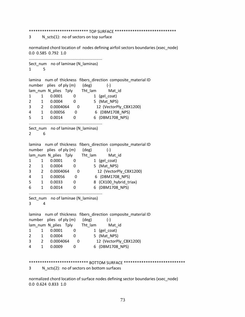
73

*************************** TOP SURFACE **************************** 3 N_scts(1): no of sectors on top surface normalized chord location of nodes defining airfoil sectors boundaries (xsec_node) 0.0 0.585 0.792 1.0 .................................................................. Sect_num no of laminae (N_laminas) 1 5 lamina num of thickness fibers_direction composite_material ID number plies of ply (m) (deg) (-) lam_num N_plies Tply Tht_lam Mat_id 1 1 0.0001 0 1 (gel_coat) 2 1 0.0004 0 5 (Mat_NPS) 3 2 0.0004064 0 12 (VectorPly_CBX1200) 4 1 0.00056 0 6 (DBM1708_NPS) 5 1 0.0014 0 6 (DBM1708_NPS) .................................................................. Sect_num no of laminae (N_laminas) 2 6 lamina num of thickness fibers_direction composite_material ID number plies of ply (m) (deg) (-) lam_num N_plies Tply Tht_lam Mat_id 1 1 0.0001 0 1 (gel_coat) 2 1 0.0004 0 5 (Mat_NPS) 3 2 0.0004064 0 12 (VectorPly_CBX1200) 4 1 0.00056 0 6 (DBM1708_NPS) 5 1 0.0033 0 8 (CX100_hybrid_triax) 6 1 0.0014 0 6 (DBM1708_NPS) .................................................................. Sect_num no of laminae (N_laminas) 3 4 lamina num of thickness fibers_direction composite_material ID number plies of ply (m) (deg) (-) lam_num N_plies Tply Tht_lam Mat_id 1 1 0.0001 0 1 (gel_coat) 2 1 0.0004 0 5 (Mat_NPS) 3 2 0.0004064 0 12 (VectorPly_CBX1200) 4 1 0.0009 0 6 (DBM1708_NPS) *************************** BOTTOM SURFACE **************************** 3 N_scts(2): no of sectors on bottom surfaces normalized chord location of surface nodes defining sector boundaries (xsec_node) 0.0 0.624 0.833 1.0

74

.................................................................. Sect_num no of laminae (N_laminas) 1 5 lamina num of thickness fibers_direction composite_material ID number plies of ply (m) (deg) (-) lam_num N_plies Tply Tht_lam Mat_id 1 1 0.0001 0 1 (gel_coat) 2 1 0.0004 0 5 (Mat_NPS) 3 2 0.0004064 0 12 (VectorPly_CBX1200) 4 1 0.00056 0 6 (DBM1708_NPS) 5 1 0.0014 0 6 (DBM1708_NPS) .................................................................. Sect_num no of laminae (N_laminas) 2 6 lamina num of thickness fibers_direction composite_material ID number plies of ply (m) (deg) (-) lam_num N_plies Tply Tht_lam Mat_id 1 1 0.0001 0 1 (gel_coat) 2 1 0.0004 0 5 (Mat_NPS) 3 2 0.0004064 0 12 (VectorPly_CBX1200) 4 1 0.00056 0 6 (DBM1708_NPS) 5 1 0.0033 0 8 (CX100_hybrid_triax) 6 1 0.0014 0 6 (DBM1708_NPS) .................................................................. Sect_num no of laminae (N_laminas) 3 4 lamina num of thickness fibers_direction composite_material ID number plies of ply (m) (deg) (-) lam_num N_plies Tply Tht_lam Mat_id 1 1 0.0001 0 1 (gel_coat) 2 1 0.0004 0 5 (Mat_NPS) 3 2 0.0004064 0 12 (VectorPly_CBX1200) 4 1 0.0009 0 6 (DBM1708_NPS)

75

Station 7.1 (cutout)

Overall Blade-sections-specific data -------------------------------------- Sec span l.e. chord aerodynamic af_shape int str layup location position length twist file file Span_loc Le_loc Chord Tw_aero Af_shape_file Int_str_file (-) (-) (m) (degrees) (-) (-) 0.000000 0.640000 0.09500 0.250000 'shape7.1.inp' 'layup7.1.inp' 1.000000 0.640000 0.09500 0.250000 'shape7.1.inp' 'layup7.1.inp' Webs (spars) data -------------------------------------------------- 1 Nweb : number of webs (-) ! enter 0 if the blade has no webs 1 Ib_sp_stn : blade station number where inner-most end of webs is located (-) 2 Ob_sp_stn : blade station number where outer-most end of webs is located (-) Web_num Inb_end_ch_loc Oub_end_ch_loc (fraction of chord length) 1 1.0 1.0

Layup (web present but not shown here) Composite laminae lay-up inside the blade section

0 0.1 0.2 0.3 0.4 0.5 0.6 0.7 0.8 0.9 1

-0.3

-0.2

-0.1

0

0.1

0.2

0.3

0.4

shape7.1.inp

76

*************************** TOP SURFACE **************************** 3 N_scts(1): no of sectors on top surface normalized chord location of nodes defining airfoil sectors boundaries (xsec_node) 0.0 0.74 0.884 1.0 .................................................................. Sect_num no of laminae (N_laminas) 1 5 lamina num of thickness fibers_direction composite_material ID number plies of ply (m) (deg) (-) lam_num N_plies Tply Tht_lam Mat_id 1 1 0.0001 0 1 (gel_coat) 2 1 0.0004 0 5 (Mat_NPS) 3 2 0.0004064 0 12 (VectorPly_CBX1200) 4 1 0.00056 0 6 (DBM1708_NPS) 5 1 0.0014 0 6 (DBM1708_NPS) .................................................................. Sect_num no of laminae (N_laminas) 2 6 lamina num of thickness fibers_direction composite_material ID number plies of ply (m) (deg) (-) lam_num N_plies Tply Tht_lam Mat_id 1 1 0.0001 0 1 (gel_coat) 2 1 0.0004 0 5 (Mat_NPS) 3 2 0.0004064 0 12 (VectorPly_CBX1200) 4 1 0.00056 0 6 (DBM1708_NPS) 5 1 0.0033 0 8 (CX100_hybrid_triax) 6 1 0.0014 0 6 (DBM1708_NPS) .................................................................. Sect_num no of laminae (N_laminas) 3 4 lamina num of thickness fibers_direction composite_material ID number plies of ply (m) (deg) (-) lam_num N_plies Tply Tht_lam Mat_id 1 1 0.0001 0 1 (gel_coat) 2 1 0.0004 0 5 (Mat_NPS) 3 2 0.0004064 0 12 (VectorPly_CBX1200) 4 1 0.0009 0 6 (DBM1708_NPS) *************************** BOTTOM SURFACE **************************** 3 N_scts(2): no of sectors on bottom surfaces normalized chord location of surface nodes defining sector boundaries (xsec_node) 0.0 0.873 0.96 1.0

77

.................................................................. Sect_num no of laminae (N_laminas) 1 5 lamina num of thickness fibers_direction composite_material ID number plies of ply (m) (deg) (-) lam_num N_plies Tply Tht_lam Mat_id 1 1 0.0001 0 1 (gel_coat) 2 1 0.0004 0 5 (Mat_NPS) 3 2 0.0004064 0 12 (VectorPly_CBX1200) 4 1 0.00056 0 6 (DBM1708_NPS) 5 1 0.0014 0 6 (DBM1708_NPS) .................................................................. Sect_num no of laminae (N_laminas) 2 6 lamina num of thickness fibers_direction composite_material ID number plies of ply (m) (deg) (-) lam_num N_plies Tply Tht_lam Mat_id 1 1 0.0001 0 1 (gel_coat) 2 1 0.0004 0 5 (Mat_NPS) 3 2 0.0004064 0 12 (VectorPly_CBX1200) 4 1 0.00056 0 6 (DBM1708_NPS) 5 1 0.0033 0 8 (CX100_hybrid_triax) 6 1 0.0014 0 6 (DBM1708_NPS) .................................................................. Sect_num no of laminae (N_laminas) 3 4 lamina num of thickness fibers_direction composite_material ID number plies of ply (m) (deg) (-) lam_num N_plies Tply Tht_lam Mat_id 1 1 0.0001 0 1 (gel_coat) 2 1 0.0004 0 5 (Mat_NPS) 3 2 0.0004064 0 12 (VectorPly_CBX1200) 4 1 0.0009 0 6 (DBM1708_NPS)

78

Station 8.1 Overall Blade-sections-specific data -------------------------------------- Sec span l.e. chord aerodynamic af_shape int str layup location position length twist file file Span_loc Le_loc Chord Tw_aero Af_shape_file Int_str_file (-) (-) (m) (degrees) (-) (-) 0.000000 0.640000 0.0600 0.0000 'shape7.1.inp' 'layup7.1.inp' 1.000000 0.640000 0.0600 0.0000 'shape7.1.inp' 'layup7.1.inp' Webs (spars) data -------------------------------------------------- 1 Nweb : number of webs (-) ! enter 0 if the blade has no webs 1 Ib_sp_stn : blade station number where inner-most end of webs is located (-) 2 Ob_sp_stn : blade station number where outer-most end of webs is located (-) Web_num Inb_end_ch_loc Oub_end_ch_loc (fraction of chord length) 1 1.0 1.0

Layup (web present but not shown here) Same as Station 7.1

79

APPENDIX E: SMART BLADE LAYUP Low Pressure

(B)

(B.1)

(B.2)

(F.1)

80

(F.2)

(G)

High pressure

(B)

(B.1)

81

(B.2)

(F.1)

(F.2)

(G)

82

APPENDIX F: INFLOW AND TURBINE INSTRUMENTATION

Table F.1 Inflow Instrumentation

Name Instrument Location Placement

BAHHATIU

Ultrasonic Anemometer

Center Met Tower

Hub Height

BAHHATIV

BAHHATIW

BAHHATIT

BAHHC Cup

BAHHV Wind Vane

BARTC Cup Rotor Top

BARBC Cup Rotor Bottom

BA2mC Cup 2m

BATP Temperature 2m

BADTP Differential Temperature

Hub Height

BAHHEC Cup Near South Met Tower

BAHHWC Cup Near North Met Tower

OHHC Cup Off-Axis Met Tower

OHHV Wind Vane

BAROMETRIC_PRESSURE Barometric Pressure Instrument Building 2m

Table F.2 Turbine Instrumentation

Name Instrument Location Placement

On_Off Turbine Monitor Tower Base

GENERATOR_POWER Turbine Power

PLC_BRAKE_M Maintenance Brake Monitor Tower Base

PLC_BRAKE_E Emergency Brake Monitor

YAW_ANGLE Yaw Position

Nacelle

AZIMUTH_ANGLE Rotor Azimuth

ROTATIONAL_SPEED Rotor Speed

LSS_SPEED Rotor Speed, Magnetic Encoder

NACELLE_IMU_AX Fore-Aft Acceleration

NACELLE_IMU_AY Side-to-Side Acceleration

NACELLE_IMU_AZ Up-Down Acceleration

NACELLE_IMU_RX Pitch Rate

NACELLE_IMU_RY Roll Rate

NACELLE_IMU_RZ Yaw Rate

BTNACC Wind Speed Cup

TOWER_BENDING_FA Fore-Aft Bending Tower 12 Feet

TOWER_BENDING_SS Side-to-Side Bending

83

Table F.3 Rotor Instrumentation

Name Instrument Location Placement

Bn_Strain_0350_Z_TE Root Edge Bending

Blade n, where n = 1,2,3

Root Bn_Strain_0350_Z_LE

Bn_Strain_0350_Z_HP Root Flap Bending Root

Bn_Strain_0350_Z_LP

Bn_Strain_2250_Z_LP Flap Bending - 1/4 span 2250 mm

Bn_Strain_4500_Z_LP Flap Bending - 1/2 span 4500 mm

Bn_Strain_6750_Z_LP Flap Bending - 3/4 span 6750 mm

Hn_Strain_Z_Flap Hub Flap Bending Hub

Hn_Strain_Z_Edge Hub Edge Bending

Bn_Accel_2000_X_HP

Tri-axial Accelorometer

Blade n, where n = 1,2,3

2000 mm, Centerline

Bn_Accel_2000_Y_HP

Bn_Accel_2000_Z_HP

Bn_Accel_2000_X_TE Uni-axial Accelorometer 2000 mm, Offset

Bn_Accel_8000_X_HP

Tri-axial Accelorometer 8000 mm Bn_Accel_8000_Y_HP

Bn_Accel_8000_Z_HP

Bn_Accel_8000_X_TE Uni-axial Accelorometer 8000 mm

Bn_FBGT_0350_Z_LP Fiber Optic Temperature

Blade n, where n = 1,2,3

Root

Bn_FBGT_2250_Z_LP Fiber Optic Temperature 2250 mm

Bn_FBGT_4500_Z_LP Fiber Optic Temperature 4500 mm

Bn_FBGT_6750_Z_LP Fiber Optic Temperature 6750 mm

Bn_FBGS_6750_Z_LP Fiber Optic Strain, flap 6750 mm

Bn_FBGS_4500_Z_LP Fiber Optic Strain, flap 4500 mm

Bn_FBGS_2250_Z_LP Fiber Optic Strain, flap 2250 mm

Bn_FBGS_0350_Z_LP Fiber Optic Strain, flap

Root

Bn_FBGS_0350_Z_LE Fiber Optic Strain, edge

Bn_FBGT_0350_Z_HP Fiber Optic Temperature

Bn_FBGS_0350_Z_HP Fiber Optic Strain, flap

Bn_FBGS_0350_Z_TE Fiber Optic Strain, edge

Bn_Motor1_Position Flap 1, motor position

Blade n, where n = 1,2,3

7330 mm Bn_Motor1_Current Flap 1, motor current

Bn_Motor2_Position Flap 2, motor position 7940 mm

Bn_Motor2_Current Flap 2, motor current

Bn_Motor3_Position Flap 3, motor position 8550 mm

Bn_Motor3_Current Flap 3, motor current

Athena_AnalogOut1 Blade 1 command

Control Enclosure Hub Athena_AnalogOut2 Blade 2 command

Athena_AnalogOut3 Blade 3 command

DAQ_IMU_X

Rotor Acceleration DAQ Enclosure Hub Center DAQ_IMU_Y

DAQ_IMU_Z

84

APPENDIX G: DATA FILE SUMMARIES

Table G.1 Initial shakedown.

Data File Time Stamp LabelMean Wind

Speed (m/s)

Median Wind

Direction (deg)

Event

TimeTurbine State AAD State Change

2012-02-01-20-55-49.zip 'Wed, Feb 01, 2012 2:55:49 PM' 6.4 331 14:57:30 parked homing

15:05:20 slow roll, start

2012-02-01-21-05-52.zip 'Wed, Feb 01, 2012 3:05:53 PM' 6.0 343 15:06:45 slow roll, stop

15:08:15 parked sine(5deg,1Hz)

15:09:15 parked stopped

2012-02-01-21-19-45.zip 'Wed, Feb 01, 2012 3:19:46 PM' 5.4 24 15:20:45 parked homing

15:22:20 parked homing

15:23:40 parked homing

15:26:09 parked sine(10deg,1Hz)

15:27:07 parked stopped

2012-02-01-22-42-36.zip 'Wed, Feb 01, 2012 4:42:36 PM' 5.5 15 16:42:55 slow roll, start

16:44:30 slow roll, stop

2012-02-01-22-50-31.zip 'Wed, Feb 01, 2012 4:50:32 PM' 3.5 22 16:53:30 slow roll, start

16:56:00 slow roll, stop

16:59:10 parked homing

17:00:00 slow roll, start

2012-02-01-23-00-34.zip 'Wed, Feb 01, 2012 5:00:35 PM' 3.9 21 17:00:55 turning sine(10deg,1Hz)

17:02:45 slow roll, stop

17:03:05 parked stopped

2012-02-01-23-10-34.zip 'Wed, Feb 01, 2012 5:10:35 PM' 4.3 13 parked

2012-02-10-17-13-42.zip 'Fri, Feb 10, 2012 11:13:42 AM' 2.5 331 11:14:00 parked sine(10deg,1Hz)

11:16:00 parked stopped

11:17:00 parked B1: sine sweep(10deg)

2012-02-10-17-23-47.zip 'Fri, Feb 10, 2012 11:23:48 AM' 1.8 55 11:26:00 parked stopped

11:28:00 parked sine sweep(10deg)

2012-02-10-17-33-45.zip 'Fri, Feb 10, 2012 11:33:46 AM' 1.9 317 11:38:00 parked stopped

2012-02-10-17-43-45.zip 'Fri, Feb 10, 2012 11:43:45 AM' 1.6 251 11:43:45 parked sine series(10deg)

2012-02-10-17-53-50.zip 'Fri, Feb 10, 2012 11:53:50 AM' 1.6 38 11:54:00 parked stopped

2012-02-10-18-59-59.zip 'Fri, Feb 10, 2012 12:59:59 PM' 2.3 298 13:02:00 parked steps(5deg,20s)

13:03:30 slow roll, start

13:06:45 slow roll, stop

13:07:00 parked stopped

2012-02-10-19-10-02.zip 'Fri, Feb 10, 2012 1:10:03 PM' 1.9 308 parked

85

Table G.2 First operation during power production.

Data File Time Stamp LabelMean Wind

Speed (m/s)

Median Wind

Direction (deg)

Event

TimeTurbine State AAD State Change

2012-02-21-14-49-46.zip 'Tue, Feb 21, 2012 8:49:47 AM' 7.8 248 8:51:00 parked sine(10deg,1Hz)

8:59:45 parked stopped

2012-02-21-14-59-50.zip Tue, Feb 21, 2012 8:59:51 AM' 7.7 255 9:00:30 starting

9:02:20 generating

2012-02-21-15-09-50.zip 'Tue, Feb 21, 2012 9:09:51 AM' 9.2 258 9:11:00 generating steps(5deg,20s)

2012-02-21-15-19-51.zip 'Tue, Feb 21, 2012 9:19:52 AM' 10.2 264 9:20:20 generating stopped

9:21:30 generating steps(5deg,40s)

9:29:50 generating stopped

2012-02-21-15-29-51.zip 'Tue, Feb 21, 2012 9:29:52 AM' 11 264 9:31:30 generating steps(10deg,30s)

2012-02-21-15-39-51.zip 'Tue, Feb 21, 2012 9:39:51 AM' 11.6 262 9:41:20 generating stopped

9:43:10 stopping

2012-02-21-15-49-50.zip 'Tue, Feb 21, 2012 9:49:50 AM' 10.5 271 parked

2012-02-29-18-31-09.zip 'Wed, Feb 29, 2012 12:31:10 PM' 3.9 224 12:31:00 parked homing

12:33:00 parked sine(5deg,1Hz)

12:35:40 parked stopped

2012-02-29-18-41-09.zip 'Wed, Feb 29, 2012 12:41:09 PM' 2.4 219 parked

2012-02-29-18-48-56.zip 'Wed, Feb 29, 2012 12:48:56 PM' 4.5 187 12:50:30 parked homing

12:52:10 parked sine(5deg,1Hz)

12:56:50 parked stopped

2012-02-29-18-58-59.zip 'Wed, Feb 29, 2012 12:58:59 PM' 4.5 197 parked

2012-02-29-19-08-59.zip 'Wed, Feb 29, 2012 1:08:59 PM' 4.5 201 13:14:20 parked static 0deg flap

13:17:30 parked stopped

2012-02-29-19-18-59.zip 'Wed, Feb 29, 2012 1:18:59 PM' 5.9 203 13:24:30 parked homing

2012-02-29-19-28-59.zip 'Wed, Feb 29, 2012 1:28:59 PM' 4.7 190 parked

2012-02-29-19-44-50.zip 'Wed, Feb 29, 2012 1:44:50 PM' 5.2 185 parked

2012-02-29-19-54-53.zip 'Wed, Feb 29, 2012 1:54:53 PM' 5.1 186 14:01:25 parked homing

2012-02-29-20-04-53.zip 'Wed, Feb 29, 2012 2:04:53 PM' 5.6 189 14:11:30 parked

2012-02-29-20-14-53.zip 'Wed, Feb 29, 2012 2:14:53 PM' 6 195 14:18:25 parked homing

2012-02-29-20-24-53.zip 'Wed, Feb 29, 2012 2:24:53 PM' 5.1 193 parked

2012-02-29-20-34-52.zip 'Wed, Feb 29, 2012 2:34:53 PM' 6.1 213 14:36:15 parked homing

14:40:05 parked homing

14:40:30 parked homing

14:44:45 parked homing

2012-02-29-20-44-52.zip 'Wed, Feb 29, 2012 2:44:53 PM' 7.6 208 14:50:25 parked sine(5deg,1Hz)

14:52:05 parked stopped

14:52:30 parked homing

14:53:15 parked sine(5deg,1Hz)

2012-02-29-20-54-53.zip 'Wed, Feb 29, 2012 2:54:53 PM' 7.9 212 14:59:20 parked stopped

86

Table G.3 Static flap settings with 10-minute data files.

Data File Time Stamp LabelMean Wind

Speed (m/s)

Median Wind

Direction (deg)

Event

TimeTurbine State AAD State Change

2012-03-09-15-19-51.zip 'Fri, Mar 09, 2012 9:19:52 AM' CORRECTING STRAIN OFFSETS - SIGNALS ARE IN RAW COUNTS

2012-03-14-16-37-33.zip 'Wed, Mar 14, 2012 11:37:33 AM' 8.2 220 11:37:45 starting

11:38:45 generating

11:40:20 generating steps(15deg,20s)

2012-03-14-16-47-37.zip 'Wed, Mar 14, 2012 11:47:38 AM' 7.6 216 11:48:20 generating stopped

11:48:40 generating steps(20deg,20s)

2012-03-14-16-57-37.zip 'Wed, Mar 14, 2012 11:57:38 AM' 7.7 221 11:58:15 generating stopped

11:59:05 stopping

2012-03-14-17-07-36.zip 'Wed, Mar 14, 2012 12:07:37 PM' 7.5 216 parked

2012-03-14-17-17-36.zip 'Wed, Mar 14, 2012 12:17:36 PM' 7.6 222 12:20:40 parked static 0deg flap

2012-03-14-17-27-36.zip 'Wed, Mar 14, 2012 12:27:37 PM' 7.8 224 parked

2012-03-14-17-37-36.zip 'Wed, Mar 14, 2012 12:37:37 PM' 8.6 221 parked

2012-03-14-17-47-36.zip 'Wed, Mar 14, 2012 12:47:37 PM' 8.6 221 12:56:25 parked stopped

12:56:40 parked sine(10deg,1Hz)

12:57:20 parked stopped

12:57:30 parked static 0deg flap

2012-03-14-17-57-40.zip 'Wed, Mar 14, 2012 12:57:41 PM' 7.8 222 12:58:10 starting

12:59:00 generating

12:59:10 generating stopped

13:00:30 generating step series(2P)

2012-03-14-18-07-37.zip 'Wed, Mar 14, 2012 1:07:38 PM' 8 219 generating

2012-03-14-18-17-37.zip 'Wed, Mar 14, 2012 1:17:38 PM' 7.8 215 generating

2012-03-14-18-27-37.zip 'Wed, Mar 14, 2012 1:27:38 PM' 7.3 214 generating

2012-03-14-18-37-37.zip 'Wed, Mar 14, 2012 1:37:38 PM' 7.2 211 generating

2012-03-14-18-47-37.zip 'Wed, Mar 14, 2012 1:47:38 PM' 7.2 212 generating

2012-03-14-18-57-37.zip 'Wed, Mar 14, 2012 1:57:38 PM' 7.3 201 14:00:25 generating stopped

14:01:45 generating static 0deg flap

2012-03-14-19-07-38.zip 'Wed, Mar 14, 2012 2:07:38 PM' 7.4 197 generating

2012-03-14-19-17-38.zip 'Wed, Mar 14, 2012 2:17:38 PM' 8.2 198 generating

14:27:20 generating stopped

2012-03-14-19-27-37.zip 'Wed, Mar 14, 2012 2:27:38 PM' 8.2 191 14:27:45 generating static -10deg flap

14:37:45 generating stopped

2012-03-14-19-37-37.zip 'Wed, Mar 14, 2012 2:37:38 PM' 7.2 195 14:37:55 generating static -20deg flap

14:45:20 generating stopped

14:46:55 generating static 10deg flap

2012-03-14-19-47-37.zip 'Wed, Mar 14, 2012 2:47:38 PM' 8.4 189 14:57:15 generating stopped

2012-03-14-19-57-37.zip 'Wed, Mar 14, 2012 2:57:38 PM' 8.1 200 14:57:40 generating static 20deg flap

2012-03-14-20-07-37.zip 'Wed, Mar 14, 2012 3:07:38 PM' 8.3 197 15:07:50 generating stopped

15:08:25 generating static 15deg flap

15:17:15 generating stopped

2012-03-14-20-17-38.zip 'Wed, Mar 14, 2012 3:17:38 PM' 8.1 209 15:17:40 generating static -15deg flap

15:27:30 generating stopped

2012-03-14-20-27-38.zip 'Wed, Mar 14, 2012 3:27:38 PM' 7.6 205 15:27:40 generating static -5deg flap

2012-03-14-20-37-37.zip 'Wed, Mar 14, 2012 3:37:38 PM' 7.5 199 15:38:10 generating stopped

15:38:20 generating static 5deg flap

15:47:35 generating stopped

2012-03-14-20-47-37.zip 'Wed, Mar 14, 2012 3:47:38 PM' 7.5 225 15:45:45 generating static 0deg flap

15:54:45 generating stopped

15:56:50 generating sine steps 5deg

2012-03-14-20-57-37.zip 'Wed, Mar 14, 2012 3:57:38 PM' 7.5 222 16:06:50 generating stopped

16:07:25 stopping

2012-03-14-21-07-38.zip 'Wed, Mar 14, 2012 4:07:38 PM' 7.1 202 16:07:45 parked sine(10deg,1Hz)

16:16:45 parked stopped

2012-03-14-21-17-37.zip 'Wed, Mar 14, 2012 4:17:37 PM' 8.9 219 parked off

87

Table G.4 Sine sweeps during power production.

Data File Time Stamp LabelMean Wind

Speed (m/s)

Median Wind

Direction (deg)

Event

TimeTurbine State AAD State Change

2012-04-09-15-23-23.zip Mon, Apr 09, 2012 10:23:23 AM 9.6 213 10:24:06 parked sine(10deg, 1Hz)

2012-04-09-15-24-29.zip Mon, Apr 09, 2012 10:24:30 AM 9.2 213 10:25:15 parked stopped

2012-04-09-15-25-24.zip Mon, Apr 09, 2012 10:25:24 AM 9.4 212 10:25:43 startup attempt

10:26:06 starting

2012-04-09-15-26-23.zip Mon, Apr 09, 2012 10:26:23 AM 9.4 214 10:26:57 generating off

2012-04-09-15-27-23.zip Mon, Apr 09, 2012 10:27:23 AM 8.1 209 generating off

2012-04-09-15-28-23.zip Mon, Apr 09, 2012 10:28:24 AM 7.3 214 generating off

2012-04-09-15-29-26.zip Mon, Apr 09, 2012 10:29:26 AM 6.8 212 generating off

2012-04-09-15-30-23.zip Mon, Apr 09, 2012 10:30:24 AM 8.2 218 10:31:00 generating sine sweep(10deg, 250s)

2012-04-09-15-31-23.zip Mon, Apr 09, 2012 10:31:24 AM 7.3 216 generating

2012-04-09-15-32-23.zip Mon, Apr 09, 2012 10:32:24 AM 7.1 212 generating

2012-04-09-15-33-23.zip Mon, Apr 09, 2012 10:33:24 AM 9.5 211 generating

2012-04-09-15-34-23.zip Mon, Apr 09, 2012 10:34:24 AM 7.8 211 10:35:15 generating stopped

2012-04-09-15-35-23.zip Mon, Apr 09, 2012 10:35:24 AM 8.9 215 generating

2012-04-09-15-36-23.zip Mon, Apr 09, 2012 10:36:24 AM 9.1 212 generating

2012-04-09-15-37-23.zip Mon, Apr 09, 2012 10:37:24 AM 8.9 213 generating

2012-04-09-15-38-23.zip Mon, Apr 09, 2012 10:38:24 AM 8.6 214 generating

2012-04-09-15-39-23.zip Mon, Apr 09, 2012 10:39:24 AM 7.8 203 generating

2012-04-09-15-39-55.zip Mon, Apr 09, 2012 10:39:56 AM 8.3 213 10:40:06 generating sine sweep(15deg, 250s)

10:44:30 generating stopped

2012-04-09-15-50-01.zip Mon, Apr 09, 2012 10:50:01 AM 8.8 211 10:51:28 generating sine sweep(15deg, 500s)

11:00:00 generating stopped

2012-04-09-16-00-01.zip Mon, Apr 09, 2012 11:00:02 AM 9.4 211 generating

2012-04-09-16-10-01.zip Mon, Apr 09, 2012 11:10:01 AM 8.9 213 11:10:12 generating attempt step series(2P)

11:11:20 generating stopped

11:14:06 generating attempt static 0deg

11:16:15 generating stopped

11:16:48 generating attempt sine(10deg, 1Hz)

11:17:47 generating stopped

11:19:06 generating attempt static 0deg

2012-04-09-16-20-01.zip Mon, Apr 09, 2012 11:20:01 AM 8.5 214 11:21:44 stopping

11:22:26 parked stopped

11:24:25 parked attempt sine(10deg, 1Hz)

2012-04-09-16-30-00.zip Mon, Apr 09, 2012 11:30:00 AM 8.8 214 parked off

88

Table G.5 Power production at prevailing wind direction with flap step series.

Data File Time Stamp LabelMean Wind

Speed (m/s)

Median Wind

Direction (deg)

Event

TimeTurbine State AAD State Change

2012-04-24-14-45-49.zip Tue, Apr 24, 2012 9:45:50 AM 9.1 234 9:48:00 parked sine(10deg, 1Hz)

9:48:45 parked stopped

9:50:10 startup attempt

9:51:19 starting

9:51:54 generating

9:52:49 generating step series(10s)

9:54:22 generating stopped

2012-04-24-14-55-54.zip Tue, Apr 24, 2012 9:55:55 AM 8.7 234 10:02:14 generating step series(30s)

2012-04-24-15-05-55.zip Tue, Apr 24, 2012 10:05:55 AM 9.1 236 generating

2012-04-24-15-15-55.zip Tue, Apr 24, 2012 10:15:56 AM 8.7 237 generating

2012-04-24-15-25-55.zip Tue, Apr 24, 2012 10:25:56 AM 7.6 227 generating

2012-04-24-15-35-55.zip Tue, Apr 24, 2012 10:35:56 AM 7.5 227 generating

2012-04-24-15-45-55.zip Tue, Apr 24, 2012 10:45:56 AM 7.7 221 generating

2012-04-24-15-55-55.zip Tue, Apr 24, 2012 10:55:56 AM 7.8 224 generating

2012-04-24-16-05-55.zip Tue, Apr 24, 2012 11:05:56 AM 7.7 216 generating

2012-04-24-16-15-55.zip Tue, Apr 24, 2012 11:15:55 AM 7.2 209 generating

2012-04-24-16-25-55.zip Tue, Apr 24, 2012 11:25:56 AM 7.8 206 generating

2012-04-24-16-35-55.zip Tue, Apr 24, 2012 11:35:55 AM 7.2 209 generating

2012-04-24-16-45-55.zip Tue, Apr 24, 2012 11:45:55 AM 7.1 208 generating

2012-04-24-16-55-55.zip Tue, Apr 24, 2012 11:55:55 AM 7.5 205 generating

2012-04-24-17-05-55.zip Tue, Apr 24, 2012 12:05:55 PM 8.5 205 generating

2012-04-24-17-15-55.zip Tue, Apr 24, 2012 12:15:55 PM 8.5 205 generating

2012-04-24-17-25-55.zip Tue, Apr 24, 2012 12:25:55 PM 9 194 generating

2012-04-24-17-35-55.zip Tue, Apr 24, 2012 12:35:55 PM 8.9 200 generating

2012-04-24-17-45-55.zip Tue, Apr 24, 2012 12:45:55 PM 9.9 203 generating

2012-04-24-17-55-55.zip Tue, Apr 24, 2012 12:55:56 PM 9.3 207 generating

2012-04-24-18-05-55.zip Tue, Apr 24, 2012 1:05:55 PM 9.9 200 generating

2012-04-24-18-15-55.zip Tue, Apr 24, 2012 1:15:55 PM 9.9 200 generating

2012-04-24-18-25-55.zip Tue, Apr 24, 2012 1:25:55 PM 10 203 generating

2012-04-24-18-35-55.zip Tue, Apr 24, 2012 1:35:56 PM 9.8 212 generating

2012-04-24-18-45-55.zip Tue, Apr 24, 2012 1:45:56 PM 9.9 204 generating

2012-04-24-18-55-55.zip Tue, Apr 24, 2012 1:55:56 PM 9.5 208 generating

13:59:58 generating stopped

2012-04-24-19-05-55.zip Tue, Apr 24, 2012 2:05:55 PM 9 226 generating

2012-04-24-19-15-55.zip Tue, Apr 24, 2012 2:15:55 PM 9.5 226 generating

2012-04-24-19-25-55.zip Tue, Apr 24, 2012 2:25:55 PM 9.1 211 generating

2012-04-24-19-35-55.zip Tue, Apr 24, 2012 2:35:56 PM 8.9 216 generating

2012-04-24-19-45-55.zip Tue, Apr 24, 2012 2:45:55 PM 8.6 207 generating

2012-04-24-19-55-55.zip Tue, Apr 24, 2012 2:55:55 PM 8.6 217 generating

2012-04-24-20-05-55.zip Tue, Apr 24, 2012 3:05:56 PM 9.1 219 generating

2012-04-24-20-15-55.zip Tue, Apr 24, 2012 3:15:55 PM 8.1 219 generating

2012-04-24-20-25-55.zip Tue, Apr 24, 2012 3:25:55 PM 8.3 230 generating

2012-04-24-20-35-55.zip Tue, Apr 24, 2012 3:35:56 PM 6.8 231 generating

2012-04-24-20-45-55.zip Tue, Apr 24, 2012 3:45:55 PM 6.5 242 generating

89

Table G.6 Power production with flap step series.

Data File Time Stamp LabelMean Wind

Speed (m/s)

Median Wind

Direction (deg)

Event

TimeTurbine State AAD State Change

2012-04-30-19-32-50.zip Mon, Apr 30, 2012 2:32:51 PM 6.1 173 14:34:02 parked sine(5deg,1Hz)

14:36:15 parked stopped

14:36:55 parked sine(20deg,1Hz)

14:38:08 parked stopped

2012-04-30-19-42-54.zip Mon, Apr 30, 2012 2:42:55 PM 7.1 164 14:45:54 parked step series(30s)

2012-04-30-19-55-18.zip Mon, Apr 30, 2012 2:55:18 PM 6.7 194 parked

2012-04-30-20-05-18.zip Mon, Apr 30, 2012 3:05:18 PM 5.9 183 15:11:06 parked stopped

2012-04-30-20-15-18.zip Mon, Apr 30, 2012 3:15:18 PM 7.6 180 parked

2012-04-30-20-25-17.zip Mon, Apr 30, 2012 3:25:18 PM 7.1 184 parked

2012-04-30-20-35-17.zip Mon, Apr 30, 2012 3:35:18 PM 6 165 15:36:15 starting static 0deg

15:37:37 generating stopped

15:39:53 generating step series(30s)

15:44:36 dip in rotor speed

2012-04-30-20-47-20.zip Mon, Apr 30, 2012 3:47:21 PM 6.7 176 generating

2012-04-30-20-57-25.zip Mon, Apr 30, 2012 3:57:26 PM 7.8 172 generating

2012-04-30-21-07-27.zip Mon, Apr 30, 2012 4:07:27 PM 6.1 182 generating stopped

16:15:20 stopping

2012-05-10-19-21-14.zip Thu, May 10, 2012 2:21:14 PM 7.5 140 14:23:45 starting static 0deg

14:24:38 generating stopped

14:25:35 generating step series(30s)

2012-05-10-19-31-19.zip Thu, May 10, 2012 2:31:20 PM 7.8 143 generating

2012-05-10-19-41-20.zip Thu, May 10, 2012 2:41:20 PM 6.7 159 generating

2012-05-10-19-51-20.zip Thu, May 10, 2012 2:51:21 PM 7.4 153 generating

2012-05-10-20-01-20.zip Thu, May 10, 2012 3:01:20 PM 6.7 140 generating

2012-05-10-20-11-20.zip Thu, May 10, 2012 3:11:20 PM 5.9 155 generating

2012-05-10-20-21-20.zip Thu, May 10, 2012 3:21:20 PM 7.4 142 generating

15:30:58 dip in rotor speed

2012-05-10-20-31-20.zip Thu, May 10, 2012 3:31:20 PM 7.7 149 generating

2012-05-10-20-41-20.zip Thu, May 10, 2012 3:41:20 PM 7.3 145 15:42:38 generating stopped

15:42:49 stopping static 0deg

2012-05-10-20-51-25.zip Thu, May 10, 2012 3:51:26 PM 7.2 146

2012-05-23-18-10-35.zip Wed, May 23, 2012 1:10:36 PM 9.7 238 parked

2012-05-23-18-38-19.zip Wed, May 23, 2012 1:38:19 PM 10.1 249 13:41:13 parked sine(20deg,1Hz)

13:42:15 parked stopped

13:43:15 starting static 0deg

13:43:49 generating stopped

13:45:13 generating step series(30s)

2012-05-23-18-48-24.zip Wed, May 23, 2012 1:48:25 PM 10 248 generating

2012-05-23-18-58-25.zip Wed, May 23, 2012 1:58:25 PM 9.5 248 generating

2012-05-23-19-08-24.zip Wed, May 23, 2012 2:08:25 PM 9.7 259 generating

2012-05-23-19-18-24.zip Wed, May 23, 2012 2:18:25 PM 9.7 239 generating

2012-05-23-19-28-24.zip Wed, May 23, 2012 2:28:25 PM 10.9 239 generating

2012-05-23-19-38-24.zip Wed, May 23, 2012 2:38:25 PM 10.1 231 generating

2012-05-23-19-48-24.zip Wed, May 23, 2012 2:48:25 PM 10.2 240 generating

2012-05-23-19-58-24.zip Wed, May 23, 2012 2:58:25 PM 11.1 247 generating

2012-05-23-20-08-24.zip Wed, May 23, 2012 3:08:25 PM 10.7 234 generating

2012-05-23-20-18-24.zip Wed, May 23, 2012 3:18:24 PM 9.9 245 generating

2012-05-23-20-28-24.zip Wed, May 23, 2012 3:28:25 PM 9.7 239 generating

2012-05-23-20-38-24.zip Wed, May 23, 2012 3:38:25 PM 10.1 224 generating

2012-05-23-20-48-24.zip Wed, May 23, 2012 3:48:25 PM 11 242 generating

2012-05-23-20-58-24.zip Wed, May 23, 2012 3:58:24 PM 11.4 237 generating

2012-05-23-21-08-24.zip Wed, May 23, 2012 4:08:25 PM 10.9 241 generating stopped

16:15:59 stopping static 0deg

2012-05-23-21-18-24.zip Wed, May 23, 2012 4:18:24 PM 10.7 241 parked stopped

90

Table G.7 Data files during video of flaps in operation.

Table G.8 Power production with tape sealing possible air gaps in flap modules.

Data File Time Stamp LabelMean Wind

Speed (m/s)

Median Wind

Direction (deg)

Event

TimeTurbine State AAD State Change

2012-05-04-15-14-36.zip Fri, May 04, 2012 10:14:37 AM 5.1 235 10:17:21 parked homing

10:18:25 parked homing

10:20:09 parked homing

10:20:42 parked homing

10:22:16 parked step series(2P)

10:23:39 parked stopped

10:24:02 parked sine series(10deg)

2012-05-04-15-25-09.zip Fri, May 04, 2012 10:25:09 AM 4.7 234 10:25:09 parked stopped

10:25:40 parked sine sweep(10deg,10s)

10:27:38 starting

10:30:40 generating

10:32:01 generating step series(2P)

10:34:34 generating stopped

10:35:04 generating sine series(10deg)

2012-05-04-15-35-10.zip Fri, May 04, 2012 10:35:11 AM 4.3 223 10:35:41 generating stopped

10:36:24 generating sine sweep(10deg,10s)

10:37:14 generating sine sweep(10deg,10s)

10:37:50 generating sine sweep(10deg,10s)

10:39:09 stopping

2012-05-04-15-45-10.zip Fri, May 04, 2012 10:45:10 AM 4.8 219 off

Data File Time Stamp LabelMean Wind

Speed (m/s)

Median Wind

Direction (deg)

Event

TimeTurbine State AAD State Change

2012-05-25-15-19-24.zip Fri, May 25, 2012 10:19:24 AM 7.3 250 10:20:55 starting taped

10:22:03 generating taped

2012-05-25-15-29-29.zip Fri, May 25, 2012 10:29:30 AM 8 247 generating taped

2012-05-25-15-39-29.zip Fri, May 25, 2012 10:39:30 AM 7.8 241 generating taped

2012-05-25-15-49-29.zip Fri, May 25, 2012 10:49:30 AM 8.4 248 generating taped

2012-05-25-15-59-29.zip Fri, May 25, 2012 10:59:30 AM 6.9 253 generating taped

11:03:27 stopping taped

2012-05-25-16-09-28.zip Fri, May 25, 2012 11:09:29 AM 6.1 250 parked taped

91

92

DISTRIBUTION

1 Shreyas Ananthan c/o Ivette Gonzalez

Office of Wind and Water Power Technologies

EE-2B Forrestal Building, U.S. DOE

1000 Independence Ave. SW

Washington, DC 20585

1 Dale Berg

12421 Chelwood Trl NE

Albuquerque, NM 87112

1 Michael Derby c/o Ivette Gonzalez

Office of Wind and Water Power Technologies

EE-2B Forrestal Building, U.S. DOE

1000 Independence Ave. SW

Washington, DC 20585

1 Mark Higgins c/o Ivette Gonzalez

Office of Wind and Water Power Technologies

EE-2B Forrestal Building, U.S. DOE

1000 Independence Ave. SW

Washington, DC 20585

1 Jose Zayas c/o Ivette Gonzalez

Office of Wind and Water Power Technologies

EE-2B Forrestal Building, U.S. DOE

1000 Independence Ave. SW

Washington, DC 20585

1 MS0899 Technical Library 9536 (electronic copy)

93