Smart Sensing Technology: A New Paradigm for Structural Health Monitoring by B.F. Spencer Jr.,1 T. Nagayama,2 J.A. Rice,3 and G.A. Agha4

1 Nathan M. and Anne M. Newmark Endowed Chair in Civil Engineering, Dept. of Civil and Environmental Engineering, University of Illinois at Urbana-Champaign, Urbana, IL 61801, USA 2 Assistant Professor, Dept. of Civil Engineering, University of Tokyo, Tokyo 113-8656, Japan 3 Ph.D. Student, Dept. of Civil and Environmental Engineering, University of Illinois at Urbana-Champaign, Urbana, IL 61801, USA 4 Professor, Dept. of Computer Science, University of Illinois at Urbana-Champaign, Urbana, IL 61801, USA

ABSTRACT The computational and wireless communication capabilities of smart sensors densely distributed over structures can provide rich information for structural monitoring. While smart sensor technology has seen substantial advances during recent years, interdisciplinary efforts to address issues in sensors, networks, and application specific algorithms are needed to realize their full potential. This paper first reports on research that addresses each of these issues and then integrates this research to provide a new structural health monitoring (SHM) system that is suitable for implementation on a network of smart sensors. Experimental verification is provided using Intel’s Imote2 installed on a three-dimensional truss structure. The Imote2 is employed herein because it has the high computational and wireless communication performance required for advanced SHM applications. The efficacy of this SHM system is then demonstrated from sensing, network, and SHM algorithm perspectives. KEYWORDS: smart sensors, structural health monitoring, damage detection, distributed computing, data aggregation 1.0 INTRODUCTION

The investment of the United States in civil infrastructure is estimated to be $20 trillion. Annual costs amount to between 8-15% of the GDP for most industrialized countries (US

Census bureau 2004; Jensen 2004). This investment is likely to increase. Indeed, much attention has been focused in recent years on the declining state of the aging infrastructure in the U.S. These concerns apply not only to civil engineering structures, such as the nation's bridges, highways, and buildings, but also to other types of structures, such as the aging fleet of aircraft currently in use by domestic and foreign airlines. The ability to continuously monitor the integrity of civil infrastructure in real-time offers the opportunity to reduce maintenance and inspection costs, while providing for increased safety to the public. Furthermore, after natural disasters, it is imperative that emergency facilities and evacuation routes, including bridges and highways, be assessed for safety. Addressing all of these issues is the objective of structural health monitoring (SHM). To efficaciously investigate damage, a dense array of sensors will be required for large civil engineering structures (Spencer et al 2004; Gao 2005). To illustrate this point, consider the task of locating a few strategic sensors in structures such as the 2 km long Akashi-Kaikyo Bridge or the 443 m tall Sears Tower in Chicago so that these sensors can detect randomly occurring damage; such a task is intractable, if not impossible. To effectively detect arbitrary damage in structures, especially complicated structures, a dense array of sensors distributed over the entire structure will be required. Some efforts have been made toward in-depth

monitoring that can provide detailed information on civil infrastructure. The Tsing Ma Bridge and Kap Shui Mun Bridge in Hong Kong are monitored with 326 channels of sensors in total, producing about 65 MB of data every hour (Wong 2004). The expense of installing traditional monitoring systems, however, has limited significantly wider-spread implementation (Farrar 2001; Celebi 2002; Lynch and Loh 2006). For example, the total system cost, including installation, of the monitoring system on the Bill Emerson Memorial Bridge in Cape Girardeau, Missouri, USA is about $1.3M for 86 accelerometers, which makes the average installed cost per sensor a little over $15,000 dollars (Hartnagel 2006). Costs for other bridge installations are of a similar magnitude. Smart sensors with wireless communication capability are reported to reduce installation effort to a great extent (Lynch et al. 2005) and help to realize a dense array of sensors. Though networks of densely deployed smart sensors have the potential to improve SHM dramatically, limited resources on smart sensors preclude direct application of traditional monitoring strategies on smart sensor networks which typically require centralized, synchronized data acquisition. Such an approach for SHM requires a tremendous amount of data to be sent to such a central station and is not scalable to large numbers of sensors. Noting that damage in structures is an intrinsically local phenomenon, SHM applications using smart sensors may be realized even for structures of substantial size. Responses from sensors close to the damaged site are expected to be more heavily influenced than those remote to the damage. If data is locally processed, communication requirement will remain reasonable. Several other characteristic of smart sensors also need to be investigated with respect to application specific requirements. For example, time synchronization accuracy may not be suitable for some applications, and packet loss may severely affect the performance of SHM systems. By understanding both the structure and the smart sensor network, implementable SHM

systems deployed on a dense array of smart sensors can be realized. This paper addresses several critical problems toward realization of a SHM system employing smart sensors. Following a brief review of smart sensors and a description of the proposed system framework, middleware services such as data aggregation, reliable communication, and synchronized sensing are presented. These services are then used to develop a scalable SHM strategy for implementation on smart sensor networks. The efficacy of this strategy is then demonstrated using Intel’s Imote2 smart sensor implemented on a three-dimensional truss structure. 2.0 SMART SENSORS The essential difference between a standard sensor and smart sensor is the latter’s flexible communication and information processing capability. Each sensor has an on-board microprocessor that can be used for digital signal processing, self-diagnostics, self-identification, and self-adaptation functions. Furthermore, all smart sensor platforms have thus far employed wireless communication technology. Some of the first efforts in developing the smart sensors for application to civil engineering structures were presented by researchers at Stanford University (Straser and Kiremidjian 1996, 1998; Kiremidjian et al. 1997). Since these early efforts, numerous researchers have developed smart sensing platforms. Lynch and Loh (2006) cited over 150 papers on wireless sensor networks for SHM conducted at over 50 research institutes worldwide. The first available open hardware/software smart sensor platform, which allows users to customize hardware/software for a particular application, was the Berkeley Mote. The third generation of Mote, the Mica, was released in 2001 (Hill and Culler 2002), having improved memory capacity and using a faster microprocessor than its predecessors. Subsequent improvements to the Mica platform resulted in the Mica2, Mica2Dot, and MicaZ. Moreover these sensors have been made commercially available (Crossbow 2007).

Several SHM applications with smart sensors have been studied using both scale models and full-scale structures (e.g., Lynch et al 2002; Aoki et al. 2003; Tanner et al. 2003, Chung et al. 2004; Nagayama et al. 2004; Nitta et al. 2005; Ou et al. 2005). Sensor calibration and demonstration of data acquisition and computational capability have been performed with the ultimate goal of life-long monitoring of civil infrastructure using a dense array of smart sensors. While smart sensor technology has seen substantial advances during recent years (Hill and Culler 2002; Adler et al. 2005; Kling et al. 2005), interdisciplinary research efforts to address issues in sensors, networks, and application specific algorithms are needed to realize their potential. Some identified research gaps are summarized in Table 1. 3.0 FRAMEWORK 3.1 Network topology Most of the SHM applications with smart sensors can be categorized into two groups, neither of which has fully exploited the smart sensor's capability. In the first group, the smart sensors emulate traditional wired sensors, with all data being synchronously collected for processing at a centralized location (see Figure 1a). Centralized SHM algorithms can then be applied to this data. This approach allows for direct application of a wealth of traditional SHM algorithms. As the number of smart sensors increases, however, the measurement data to be centrally collected exceeds the network bandwidth, regardless of whether homerun or hopping communication is adopted. Forwarding data to the base station may take a prohibitively long time and consume a lot of power. Introducing faster communication speeds offered by nodes with ample power sources is one approach. Chintalapudi, et al. (2006) utilizes a tiered approach, with lower tier nodes and powerful upper tier nodes. Assuming that the upper tier nodes have sufficient power, the limitation on the communication speed

among upper tier nodes is removed; power consumption at lower tier nodes is moderate. However, installing powerful nodes is sometimes impractical or can reduce the advantages of smart sensors; the need for powerful nodes with associated power sources may increase the installation cost. In terms of the network, dependency on such nodes limits the ability of the network to automatically reconfigure should a powerful node cease to function. The limited communication bandwidth and battery power hinders the application of a centralized data acquisition approach to a large smart sensor network. The second group of the algorithms assumes that each smart sensor measures and processes data independently without sharing information among the neighboring nodes (Sohn et al. 2002; Lynch et al. 2005; Nitta et al. 2005). Since only the processed data is sent back to base station, communication requirements are quite modest. Consequently, this approach is scalable to a large number of smart sensors (see Figure 1b). However, the independent node approach does not utilize available information from neighboring nodes; all spatial information (e.g., mode shapes) is discarded. The inability to incorporate spatial information limits the effectiveness of this approach. A hierarchical system is considered to resolve the limitations of these two approaches (see Figure 1c). Smart sensors are conceptually divided into interacting communities of sensors. Data processing is coordinated and distributed among sensors. The Distributed Computing Strategy for SHM (DCS) (Gao 2005) is an example of such a hierarchical SHM system. Communication and data processing in DCS take place mainly in local sensor communities, reducing requirements on transmission of large amounts of data. Structural analysis of DCS takes into account measurements at multiple locations, making use of available spatial information. The DCS has the features that make it possible to be deployed on a dense array of smart sensors. 3.2 Proposed architecture

A homogeneous configuration of hardware is chosen, as opposed to a tiered system approach employing resource demanding upper level nodes and less powerful lower level nodes. In addition to smart sensors, a PC is needed in this architecture as the interface to the users. A homogeneous configuration results in simpler programming and deployment of smart sensor nodes. Systems with homogeneous configurations can be programmed so that failure of one node does not result in failure of the system; roles of a non-functioning node can be taken over by neighboring nodes as conceptually shown in Figure 2. In terms of functionality, smart sensor nodes in the proposed system are differentiated as follows: (i) base station, (ii) manager nodes, (iii) cluster heads, and (iv) leaf nodes. All the sensors deployed on a structure, in principal, work as leaf nodes. Leaf nodes receive commands from the other nodes and perform preprogrammed tasks such as sensing, data processing, and acknowledgement. The collection of leaf nodes in a neighborhood make a local sensor community. One of the nodes in each local sensor community is assigned as a cluster head and handles most of the communication and data processing in the community. In addition to tasks inside the community, the cluster head communicates with cluster heads of neighboring communities to exchange information. One of the cluster heads also functions as the manager sensor. When intra-cluster RF communication signals reach nodes in neighboring sensor communities, the manager deals with time sharing among sensor communities to avoid RF interference. The manager also exchanges packets directly with leaf nodes to manage operations in which all the leaf nodes participate; sensing, which is triggered by the manager sensor, is an example. The base station node is the gateway between the smart sensor network and the PC. The PC, which provides the user interface, sends commands and parameters to the smart sensor networks via the base station. The PC also receives data and calculation results from the base station. While the base station can communicate directly with any node in communication range, most communication involving the base station is

routed through the manager or cluster heads, with the exception being the transmission of a large amount of data or calculation results from leaf nodes to the PC for debugging purpose. The smart sensor platform employed in this work is Intel’s Imote2 (Adler et al. 2005). The Imote2 (Figure 3) is a new smart sensor platform developed by Intel for data intensive applications. The main board of the Imote2 incorporates a low-power X-scale processor, the PXA27x, and an 802.15.4 radio (ChipCon 2420). The processor speed may be scaled based on the application demands, thereby improving its power usage efficiency. One of the important characteristics of the Imote2, which separates it from previously developed wireless sensing nodes, is the amount of data which can be stored on the node. The Imote2 has 256 KB of integrated SRAM, 32 MB of external SDRAM, and 32 MB of Strataflash memory (Intel Corporation 2005), which is particularly important for the large amount of data required for real-time, dynamic monitoring of structures. Table 2 gives a comparison of the Imote2 to the Mica2, a third generation of Mica motes developed at Berkeley. The sensors used with the Imote2 are interfaced to the main board via two connectors. This interface provides a significant amount of built-in flexibility for the type of sensors which may be utilized. Some of the options available for I/O are I2C (which allows interface to an unlimited number of channels), 3 SPI ports (serial data ports limited to one channel per port) and multiple GPIO (general purpose I/O) pins. Intel has created a basic sensor board to interface with their Imote2. This basic sensor board can measure 3-axes of acceleration, light (TSL2561), temperature, and relative humidity (SHTx). All of the sensors on this board are digital, thus no analog to digital converter (ADC) is required (Adler et al. 2005). STMicroelectronics manufactures the 3-axis digital accelerometer (LIS3L02DQ) which has a ±2g measurement range and a resolution of 12-bits or 0.97 mg (STMicroelectronics 2005a). The LIS3L02DQ’s has a built-in ADC which is followed by digital filters with selectable cutoff frequencies. These cutoff frequencies are user

defined by setting a decimation factor, which also dictates the sampling rate of the accelerometer. The sampling rate and cutoff frequency versus the decimation factor is given in Table 2, as specified by the manufacturer. The digital output interface may be either SPI or I2C (STMicroelectronics 2005b). TinyOS is employed as the operating system on many smart sensors, including the Imote2. This operating system has a small memory footprint and is therefore suited to the limited resources of wireless sensors. TinyOS has a large user community and many successful smart sensor applications. However, some features pose limitations for SHM applications. Primarily, TinyOS does not support real time operations and thus has only two types of execution threads: 1) tasks and 2) hardware event handlers. This concurrency model leaves only a small amount of control to the user in the assignment of priority to commands; execution timing cannot be arbitrarily controlled. The subsequent section will show that this feature of TinyOS must be carefully considered when designing an SHM implementation. 4.0 MIDDLEWARE SERVICE DEVELOPMENT In this section, the basic functionalities of smart sensors essential to SHM applications are studied and realized. Among these functionalities are data aggregation, reliable communication, and synchronized sensing. These functionalities are developed on the Imote2 platform. 4.1 Data aggregation The amount of data transferred in SHM applications is considerable. Long vibration records will be acquired from densely distributed smart sensors. If they are collected at a single sink node using multi-hop communication, the associated time easily exceeds the time necessary for any other smart sensor task. Distributed estimation of the correlation function has been proposed as a type of model-based data aggregation (Nagayama et al. 2006). When the excitation can be assumed to be broadband and

the structural response stationary, the correlation function between the output measurements can be used to determine modal parameters by virtue of the Natural Excitation Technique (NExT) (James et al. 1992). This data aggregation method, which is scalable to networks of a large number of smart sensors, is described herein. Correlation functions are, in practice, estimated from finite length records. Power and cross spectral density (PSD/CSD) functions are estimated first through the following relation (Bendat and Piersol 2000):

*

1

1( ) ( ) ( )dn

xy i iid

G X Yn T

ω ω ω=

= ∑ (1)

where Gxy(ω) is the CSD estimation between two stationary random process, x(t) and y(t). X(ω) and Y(ω) are the Fourier transform of x(t) and y(t); the * denotes the complex conjugate. T is the length of the sample records, xi(t) and yi(t). In estimating the spectral densities, windowing of the time histories is common practice to suppress the phenomena of spectral leakage. Window functions are multiplied by the time histories, x(t) and y(t), prior to the Fourier transform. When nd = 1, the estimate has a large random error. The random error is reduced by computing an ensemble of the estimates from nd different or partially overlapped records. The normalized RMS error ε[|Gxy(ω)|]of the spectral density function estimation is given as

1( )xyxy d

Gn

ε ωγ

⎡ ⎤ =⎣ ⎦

γxy is the coherence function between x(t) and y(t), indicating the degree of linearity between them. Through the averaging process, the estimation error is reduced. Averaging of 10-20 times is common practice. The estimated spectral densities are then converted to correlation functions by inverse Fourier transform. An implementation of correlation function estimation for a small community of sensors in a centralized data collection scheme is shown in Figure 4, where node 1 works as a reference sensor. Assuming ns nodes, including the reference node, are measuring structural responses, each node acquires data that is sent to the reference node. The reference node calculates the spectral density. This

(2)

procedure is repeated nd times and averaged. After averaging, the inverse FFT is taken to calculate the correlation function. All the calculations take place at the reference nodes. When the spectral density is estimated from discrete time history records of length N, the amount of data to be transmitted through the radio is Nxndx (ns–1). In the next scheme, data flow for correlation function estimation is examined and data transfer is reorganized to take advantage of the computational capability on each smart sensor node (see Figure 5). After the first measurement, the reference node broadcasts the time record to all the nodes. On receiving the record, each node calculates the cross spectral density between its own data and the received record. This spectral density estimate is locally stored. The nodes repeat this procedure nd times. After each measurement, the stored value is updated by taking a weighted average between the stored value and the current estimate. In this way, Eq. (1) is calculated on each node. Finally the inverse FFT is applied to the spectral density estimate locally. The resultant correlation function is sent back to the reference node. Because the subsequent modal analysis such as ERA uses, at most, half of the correlation function data length, N/2 data is sent back to the reference node from each node. The total data to be transmitted in this scheme is, therefore, Nxnd+N/2x(ns–1). As the number of nodes increases, the advantage of the second scheme, in terms of communication requirements, becomes significant. The second approach requires data transfer of O(Nx(nd+ns)), while the first one needs to transmit to the reference sensor node data of the size of O(Nxndxns). For example, a parameter set {N,nd,ns}={1024, 20,10} necessitates the second approach to transfer 25,088 data points while the first one involves transmit of 184,320 data points; the reduction factor achieved by the distributed implementation is more than seven. The distributed implementation leverages knowledge regarding the application to reduce communication requirements as well as to utilize CPU and memory efficiently in a smart sensor network.

The data communication analysis above assumes that all the nodes are in single-hop range of the reference node. This assumption is not necessarily the case for a general SHM application. However, Gao (2005) proposed a Distributed Computing Strategy (DCS) for SHM which supports this idea. Neighboring smart sensors within single-hop communication range make local sensor communities and perform SHM in the communities. In such applications, the assumption of nodes being in single-hop range of a reference node is reasonable, while data processing results such as damage location may need to be transferred to the base station using multi-hop communication. 4.2 Reliable communication RF communication is not reliable unless lost packets are specifically addressed. Packets may not be transmitted properly. When the distance between nodes is too long, packets may not reach the destination. Multiple nodes trying to send packets at the same time cause packet collisions. SHM applications employing smart sensors suffer from this packet loss. If packets carrying commands are lost, destination nodes fail to perform certain tasks. The sender is unsure whether the destination nodes have received commands. If packets carrying measurement data are lost, destination nodes cannot fully reconstruct the sender’s data. Therefore, packet loss may cause a system to be in an unknown state and may degrade measurement signals. When smart sensor applications come to involve more and more complicated internode data processing and are assigned more and more tasks by commands sent through packets, the commands need to be reliably delivered. Otherwise, smart sensors cannot assess the current state of neighboring nodes without intricate logic, resulting in extremely complicated programs. Reliable communication of short messages is clearly a necessary feature for an SHM system with complicated internode data processing. Compared to the need for reliable communication of short messages, the need to transfer large

amounts of data is not apparent. In many SHM research attempts, data loss has not been addressed, and the loss of a few data points has often been considered acceptable. The effect of data loss on SHM applications are assessed by Nagayama, et al. (2007). Packet loss is shown to degrade signals in the same way as observation noise, therefore reliable communication is preferable to maintain data quality. Also when loss of a large block of packets is expected, such as when devices using the same frequency range pass by, resending of data is preferable. A reliable communication protocol suitable for sending a large amount of data, as well as a protocol to send a single packet, is proposed. Each of these protocols supports multicast as well as unicast data transmission; SHM applications benefit from multicast transmission. One example is the distributed correlation function estimation. Multicasting of commands is commonly observed in smart sensor systems. Because of limited space, only the reliable multicast protocol for long data is briefly explained herein. The proposed reliable communication protocol is based on a modification of the Automatic Repeat reQuest (ARQ) protocol. ARQ is an error control method which repeats the sending of packets based on requests from the receiver. On reception of packets without error, the receiver replies with a positive acknowledgement (ACK). If an error is detected, the receiver sends a negative acknowledgement (NACK) and a request for retransmission. There are several ARQ protocols. The radio component on the Imote2 is in either listening mode or in transmission mode. During transmission, the Imote2 cannot receive packets. Without careful implementation of ARQ, the receiver may send acknowledgments while the sender is in transmission mode. Packet loss and retransmission are expected to be more frequent if transmission and reception are deeply interwoven. Scheduling interwoven transmission and reception may result in long wait times. In the proposed protocol, the sender transmits all the packets without expecting an acknowledgement. The receiver stores all the received data in a

buffer. Once the sender transmits the last packet of data, the sender repeatedly transmits a packet indicating the end of data until acknowledgement packets from the receivers are received. These acknowledgment packets also contain information about missing packets. Only missing packets are resent. At the end of transmitting missing packets, a packet requesting acknowledgment is sent again. If no receiver reports missing packets, the sender signals the end of data transfer to the receivers and itself, disengaging them from this round of reliable communication. In this way, the number of acknowledgement and retransmission can be greatly reduced (see Figure 6). This protocol is designed to send 64-bit double precision data, 32-bit integers, or 16-bit integers. Many ADCs on traditional data acquisition systems have a resolution less than 16 bits, supporting the need for transfer of 16-bit integer format data. Some ADCs have a resolution better than 16 bits, necessitating data transfer in 32-bit integer format. Once an acceleration record is processed, the outcome may require more bits. Onboard data processing such as FFTs and SVDs are usually performed in a double precision format. Even when the effective number of bits is smaller than 32, debugging of onboard data processing greatly benefits from transfer of double precision data; data processing results on Imote2s can be directly compared with those on a PC, which are most likely in a double precision format. Transfer of 64-bit double precision data is supported based on such needs. 4.3 Synchronized sensing Time synchronization errors in a smart sensor network can cause inaccuracy in SHM applications. Time synchronization is a middleware service common to smart sensor applications and has been widely investigated. Each smart sensor has its own local clock, which is not synchronized initially with the other sensor nodes. By communicating with the surrounding nodes, smart sensors can assess relative differences among their local clocks. For example, Mica2 motes employing the Timing-sync Protocol for Sensor Network (Ganeriwal et al. 2003) are reported to synchronize with each other to an

accuracy of 50 μsec; different algorithms and hardware resources may result in different precision. Whereas time synchronization protocols have been intensely studied, requirements on synchronization from an application perspective have not been clearly addressed. The effect of time synchronization error on SHM applications is studied by Nagayama et al. (2007). In this section, the accuracy of Flooding Time Synchronization Protocol (FTSP) (Maroti et al. 2004; Mechitov et al. 2004), realized on the Imote2, is evaluated for the SHM application. Time synchronization among smart sensors, however, does not necessarily offer synchronized measurement signals; other critical issues must be considered. Finally synchronized sensing is realized utilizing resampling. The Imote2s are programmed as follows to evaluate time synchronization error. A beacon node transmits a beacon signal every four seconds. The others eight nodes estimate global time using the beacon packet as provided in FTSP. Two seconds after the beacon signal, the beacon node sends another packet requesting replies. The receivers get time stamps of the reception of this packet and convert them to global time stamps. The receivers take turns in reporting back these time stamps. With perfect time synchronization, the time stamp of the packet reception should give the same global time at all the nodes. This procedure is repeated more than 300 times. These time stamps from the eight nodes are compared with each other. Figure 7 shows the difference in the global time stamp using one of the eight nodes as a reference. The difference is generally less than 10 μsec, indicating the time synchronization error of about 10 μsec. Scattered peaks are not necessarily indicators of large synchronization error; they may also be due to delays associated with global time stamping after the packet requesting replies are received. The time synchronization error estimated above is considered small for SHM applications. A delay of 10 μsec corresponds to 0.072 degree phase delay for a mode at 20 Hz. Even at 100 Hz, the corresponding phase delay is only 0.36

degree. While global clock estimates two seconds after sending the beacon signal are found to be accurate, local clocks drift over time. Large clock drift necessitates frequent time synchronization to maintain a certain level of accuracy. The same program is utilized to estimate clock drift. On reception of the packet requesting replies, the receivers get offsets of their own timestamps instead of global time stamps. The offsets are sent back to the beacon node and then to a PC. If the clocks on the nodes are ticking at a consistent rate, the offsets should be constant over a long period of time. This experiment, however, did not show constant offsets. Figure 8 shows the offsets of nine receiver nodes. One of them stopped responding around 45 second, exhibiting a short line on the figure. Here, the maximum clock drift among this set of Imote2 nodes is estimated to be around 50 μsec per second. This drift is small but not negligible if measurement takes a long time. For example, after a 200-second measurement, time synchronization error may become as large as 10 msec. One solution to address this clock drift problem is frequent time synchronization. The drawback of this approach is that time synchronization may not perform well when other tasks (e.g., sensing) are running. Time synchronization requires precise time stamping as previously explained. Sensing also requires precise timing and needs higher priority in execution. Scheduling more than one high priority tasks is challenging, especially for operating systems such as TinyOS which have no support for real-time control. If the time synchronization interval necessary to address the clock drift is shorter than the sensing time, a different solution must be sought. Another approach is to compensate for the difference in clock rate. The slopes of the lines in Figure 8 approximately indicate the clock drift that needs to be compensated. If time synchronization offset values can be observed for a certain amount of time, the slope can be estimated using a least squares approach.

Several issues must be addressed to achieve synchronized sensing. Issues observed on the Imote2 platform include uncertainty in sensor start-up time, difference in sampling rate among sensor nodes, and fluctuation in sampling frequency over time (Nagayama et al. 2006). These issues are addressed by resampling of measured time histories based on time stamps marked after a fixed number of data points are collected. The polyphase implementation of resampling Oppenheim et al. (1999) by an arbitrary non-integer rational factor addresses the problem of data sampled at inaccurate frequencies. The measured time history x[m] is first upsampled by about one-hundred zeros. Then, lowpass a filter h[i] is applied to yield an upsampled signal y[j]. The outcome z[k] of the resampling process is calculated by interpolating this upsampled signal.

[ ] [ ]( ) [ ]( )

[ ] [ ]( )

( )

[ ] [ ]( )

( )

/

1

/

1

1

l a

l a

u a

u a

l u j u j l

p L

l a u jm p N L

p L

u a j lm p N L

j r i

l r i

u l

z j y p p p y p p p

h p L m x m p p

h p L m x m p p

p jM l

p jM lp p

⎢ ⎥⎣ ⎦

⎡ ⎤= − +⎢ ⎥

⎢ ⎥⎣ ⎦

⎡ ⎤= − +⎢ ⎥

= − + −

= − ⋅ − +

+ − ⋅ −

= +

= +⎢ ⎥⎣ ⎦= +

∑

∑

La is the factor of upsampling, N is the length of filter coefficients, and Mr is the non-integer factor of downsampling. ⎡⎤ and ⎣⎦ represent ceiling and floor function respectively. The initial delay, represented by li, is determined based on the global timestamp and takes into account the inaccuracy in sampled timing. The factor, La /Mr, determines the rate of sampling rate conversion. The sampling rate conversion is first tested in Matlab as shown in Figure 9 and subsequently implemented on the Imote2. The resampling process implemented on the Imote2 is found to yield acceleration signals with synchronization accuracy better than 50 μsec. 5.0 EXAMPLE IMPLEMENTATION The Distributed Computing Strategy (DCS) for

SHM (Gao 2005) is implemented on Imote2s using the developed middleware services. The SHM system realized on the Imote2s is then experimentally verified using a three-dimensional truss structure. 5.1 Distributed Computing Strategy for SHM Gao (2005) proposed a Distributed Computing Strategy (DCS) for SHM that meshes well with the hierarchical architecture necessary to realize the potential of a dense network of smart sensors. The DCS approach is an extension of the DLV method (Bernal 2002) that does not require central collection of the measurement data. Instead, DCS shares data among the neighboring nodes to utilize spatial information. Due to this local data sharing with a limited number of neighboring nodes, the total amount of data to be transmitted throughout the network is kept small. Therefore, this algorithm is scalable to a large number of sensors densely deployed over large structures. While DCS does not require measurements at all the DOFs, the method’s performance is improved by sensing at many DOFs; DCS benefits from a dense array of smart sensors. Computer analysis and experimental validation on a simulated wireless network showed that DCS is a promising SHM scheme (Gao 2002). While DCS has been shown promising as an SHM algorithm for smart sensor networks, the strategy has not been implemented on smart sensor platforms. Gao (2005) explains two methods to normalize mode shapes in DCS. One of them utilizes input force measurements while the other measures only vibration outputs under known mass perturbation. Because no Imote2 sensor board with force measurement is available and because the input force of a full-scale structure is difficult to measure, DCS employing the mass perturbation method is chosen as the algorithm to be implemented. Bernal (2006) proposed a stochastic DLV (SDLV) localization approach. This variant of the DLV method does not require normalization of mode shapes. The absence of the need for normalization greatly simplifies the SHM strategy. Therefore, the SDLV approach is also implemented on networks of Imote2s.

(3)

The DCS implementation is comprised of various steps, including numerical calculation functions, middleware services, and the damage detection algorithm. The major numerical calculation functions utilized in DCS for SHM are: singular value decomposition (SVD), complex eigensolver, Fast Fourier transform (FFT), quick sort, and complex matrix inverse. These functions are either developed from scratch or functions written in C language are adapted. The performance of these functions is examined on the Imote2; execution of these functions on the Imote2 yields identical outputs as those from Matlab functions with the precision of double data type. Required middleware services for DCS include: data aggregation, reliable communication, and synchronized sensing. The services described earlier are adapted for this purpose. The algorithm to locate damage involves NExT, ERA, and DLV. These techniques are coded as C-functions and adapted to TinyOS. Implementation of DCS for SHM including these functions requires further consideration of the limited hardware resources. The memory space on the Imote2 is limited, and the CPU speed is slower than that of a PC. For example, the size of the Hankel matrix utilized in ERA may exceed the available memory space on the Imote2s. The matrix size must be limited so that the matrix fits in the available memory. Fortunately, application of DCS on a PC to experiment data has shown that modal parameters can be estimated with sufficient accuracy using a reduced-size Hankel matrix. Additionally, estimation of the stresses induced by the DLVs may involve structural analysis of the whole truss, which requires large amounts of memory and calculation time. Instead, a matrix to convert input force to stress is calculated on a PC in advance and injected to the cluster heads; cluster heads need to simply compute the product of the matrix and the DLVs rather than to run the entire structural analysis. Through these considerations, DCS can be ported to the Imote2. Imote2s are preprogrammed to autonomously accomplish the DCS. All the necessary parameters such as node ID, sensor direction, and

data length are initially injected to the network from the base station. The base station sends these parameters to the manager sensor or cluster head sensors, which forward a part of the parameters to the leaf nodes. After this parameter injection, the PC connected to the base station does not need to give input to the Imote2 network. Tasks are preassigned to each command which is sent by the reliable communication protocol. Several functionalities, which may not be necessary for complete SHM systems, are considered important for debugging purposes and are implemented as well. Measured acceleration time histories are sent back to the base station so that processing of the time history in the network can be compared to equivalent data processing on a PC. Intermediate results of DCS such as modal parameters, DLVs, and accumulated stress are also sent back to the base station for the same reason. In addition, critical communication packets among sensor nodes are directed to the base station using the multicast reliable communication protocol so that important communication is logged at the base station for debugging. These functionalities help development and performance evaluation for the smart sensor system. 5.2 Experimental setup A 5.6 m long, three-dimensional truss structure at the Smart Structures Technology Laboratory (SSTL) of the University of Illinois at Urbana-Champaign (http://sst.cee.uiuc.edu/) is employed for experimental validation (see Figure 10). The length of each bay of the truss is 0.4 m. The truss sits on two rigid supports. One end of the truss is a pinned support, and the other is a roller support. The pinned end can rotate freely with all three translations restricted. The roller end can also move in the longitudinal direction. The truss is excited vertically by a Ling Dynamic Systems permanent magnetic V408 shaker. A band-limited white noise is sent from the computer to the shaker to excite the truss structure up to 100 Hz. The shaker is connected to the bottom of the outer panel using a stinger. Ten Imote2s mounted on nodes of the truss

measure acceleration in three directions. The three axes of the Imote2 accelerometers are aligned with longitudinal, transverse and vertical directions. The acceleration data is acquired at a nominal sampling rate of 560 Hz and resampled to 280 Hz. Six Imote2s mounted on six front panel nodes of two consecutive bays of the truss constitutes a local sensor community and monitor structural damage within the bays. The ten Imote2s in total make three overlapping sensor communities. A horizontal element on the lower cord is replaced with a thinner element to simulate damage to the truss. This replacement results in 52.7 % cross section loss in elements 20 and 8 in the mass perturbation-based DCS method experiment and SDLV-based DCS method experiment, respectively (see Figure 11). The cross section loss reduces stiffness in the element and is expected to be detected as damage by the DCS method. 5.3 Experimental results Through the resampling process, measured acceleration signals are synchronized to each other. The phase of the cross spectral densities indicates the synchronization accuracy. The slope of the phase indicates time synchronization error. As shown in Figure 12, the time synchronization error is approximately 30 μsec. Modal parameters are determined from these measured acceleration signals. The NExT method is used to estimate the cross spectral densities and convert them to correlation functions. The Hanning window is employed in spectral density estimation. Figure 13 shows cross spectral densities between the vertical acceleration signal of a cluster head node and the longitudinal and vertical acceleration signals of other nodes in the community. As expected, the spectral densities estimated on the Imote2s show clear peaks corresponding to structural modes. The acceleration signals are also processed on a PC to validate the numerical operation on the Imote2s. The spectral densities estimated on the Imote2s in a distributed manner are found to be identical (within the numerical precision of

double data type) to those calculated on the PC. Natural frequencies, damping ratios, mode shapes, EMAC, initial modal amplitude, etc. are identified from the cross spectral densities by cluster head nodes running ERA. These identified parameters are numerically the same as those identified on a PC. First, the mass perturbation-based DCS method is considered. Here, the network of Imote2s installed at nodes 7, 9, 11, 13, 15, 17, 19, 21, 23, and 25 (see Figure 11) estimates the mass normalization constants prior to commencement of monitoring by measuring the acceleration responses of the truss with and without known mass perturbation. Then Imote2s are installed at nodes 8 to 13. The modal parameters identified before and after element replacement are input to the DLV method to locate the simulated damage. The normalized accumulated stress estimated by the cluster head node, node 10, is shown in Figure 14. This local sensor community monitors elements 15 to 23. The DLV method identifies damaged elements as those with small accumulated stress. Element 20, which was replaced with a thinner bar, has a normalized accumulated stress smaller than a predetermined threshold value, 0.3. While the small normalized accumulated stress successfully localized damage in this experiment, false positive/negative damage localization is sometimes observed in other cases. The damage localization algorithm is then changed to the SDLV method, and the damaged element is sought. Ten Imote2s are installed from nodes 2 to 11. Nodes 4, 6, and 8 become cluster heads and form local sensor communities around them. Each local sensor community consists of a cluster head and five surrounding nodes. Figure 15 shows the normalized accumulated stress calculated by the three adjacent cluster heads. In this experiment, element 8 is replaced with the thinner element. As shown, the Imote2s in these local sensor communities successfully detected the damaged element. The SDLV results from the respective communities are shared among neighboring cluster heads to make judgment on damage. If neighboring nodes are consistent, the damage

detection results are reported to the base station and the cluster heads switches to the sleep mode. If inconsistency is observed, the neighbors retake data and apply the series of data processing again. Figure 16 shows the report from the cluster heads to the base station after applying the SDLV-based DCS method and exchanging damaged element information among the communities. Element 8 is identified as the only damaged element. The damage localization at the three cluster heads is consistent and the flag to indicate retaking data is set to zero. 6.0 CONCLUSION A hierarchical, distributed SHM system employing smart sensors has been developed and experimentally verified on the Imote2 smart sensor platform. To realize this SHM system required various issues and algorithms to be addressed. Middleware services including data aggregation, reliable communication, and synchronized sensing were realized on Imote2s. These services as well as numerical functions and algorithms were combined to produce the SHM system. Experimental verification using the three-dimensional truss demonstrated the efficacy of the SHM system developed herein. More details about this research can be found in Nagayama (2007). 7.0 ACKNOWLEDGEMENTS The authors gratefully acknowledge the support of this research by the National Science Foundation under NSF grants CMS 03-01140 and CMS 06-00433, Dr. S.C. Liu, Program Manager. The second and third authors would also like to acknowledge the support of a Vodafone-U.S. Foundation Graduate Fellowship. 6.0 REFERENCES

Adler, R., Flanigan, M., Huang, J., Kling, R., Kushalnagar, N., Nachman, L., Wan, CY., and Yarvis, M. “Intel mote 2: an advanced platform for demanding sensor network applications.” Proc. 3rd int. conference on Embedded networked sensor systems, 298 - 298. (2005)

Aoki, S., Fujino, Y., and Abe, M. “Intelligent bridge maintenance system using MEMS and network technology.” Proc., SPIE – Smart Systems and NDE for Civil Infrastructures, 5057, 37-42. (2003)

Bendat, J. S., and Piersol, A.G. Random data: analysis and measurement procedures, John Wiley and Sons, Inc. (2000)

Bernal, D. “Load vectors for damage localization.” J. of Engineering Mechanics, 128(1), 7-14. (2002)

Bernal, D. “Flexibility-based damage localization from stochastic realization results.” J of Engineering Mechanics, 132(6), 651-658. (2006)

Celebi, M. “Seismic instrumentation of buildings (with emphasis on federal buildings).” Special GSA/USGS Project, an administrative report, United States Geological Survey, Menlo Park, CA. (2002)

Chintalapudi, K., Paek, J., Gnawali, O., Fu, T., Dantu, K., Caffrey, J., Govindan, R., and Johnson, E. “Structural Damage Detection and Localization Using NetSHM.” Proc 5th International Conference on Information Processing in Sensor Networks: Special track on Sensor Platform Tools and Design Methods for Networked Embedded Systems (IPSN/SPOTS'06), Nashville, TN, (2006)

Chung, H.-C., Enomoto, T., Shinozuka, M., Chou, P., Park, C., Yokoi, I., and Morishita, S. “Real time visualization of structural response with wireless MEMS sensors.” Proc., 13th World Conference on Earthquake Engineering, No. 121, 1-10. (2004)

Crossbow Technology, Inc. <http://www.xbow.com> (Mar. 2, 2007).

Farrar, C. R. “Historical overview of structural health monitoring.” Lecture Notes on Structural Health Monitoring using Statistical Pattern Recognition. Los Alamos Dynamics, Los Alamos, NM. (2001)

Ganeriwal, S., Kumar, R., and Srivastava, M. B. “Timing-sync protocol for sensor networks.” Proc., 1st International Conference On Embedded Networked Sensor Systems, Los Angeles, CA, 138 - 149. (2003)

Gao., Y. Structural health monitoring strategies for smart sensor networks, Ph.D. Dissertation, University of Illinois at Urbana-Champaign, IL (2005)

Hartnagel, Bryan A. Personal Communication, August 22 (2006)

Hill, J., and Culler, D. “Mica: A wireless platform for deeply embedded networks.” IEEE Micro., 22(6), 12-24. (2002)

James, G. H., Carne, T. G., Lauffer, J. P., and Nord, A. R. “Modal testing using natural excitation.” Proc., 10th Int. Modal Analysis Conference, San Diego, CA..(1992)

Jensen, S. “Summary Outlook to 2005 for the European Construction Market.” http://www.cifs.dk/scripts/artikel.asp?id=775&lng=2. (2005)

Kiremidjian, A. S., Straser, E. G., Meng, T. H., Law, K. and Soon, H. “Structural damage monitoring for civil structures.” Proc., Int. Workshop on Structural Health Monitoring, Stanford, CA, 371-382. (1997)

Kling, R., Adler, R., Huang, J., Hummel, V., and Nachman, L. “Intel Mote-based Sensor Networks.” Structural Control Health Monitoring, 12:469–479. (2005)

Lynch, J. P., Law, K. H., Kiremidjian, A. S., Carryer, E., Kenny, T. W., Patridge, A., and Sundararajan, A. “Validation of a wireless modular monitoring system for structures.” Proc., SPIE - Smart Structures and Materials: Smart Systems for Bridges, Structures, and Highways, San Diego, CA, 4696(2), 17-21. (2002)

Lynch, J. P. and Loh, K. “A summary review of wireless sensors and sensor networks for structural health monitoring.” Shock and Vibration Digest, 38(2), 91-128. (2006)

Lynch, J. P., Wang, Y., Law, K. H., Yi, J.-H., Lee, C. G., and Yun, C. B. “Validation of a large-scale wireless structural monitoring system on the Geumdang bridge.” Proc., the Int. Conference on Safety and Structural Reliability, Rome, Italy. (2005)

Maroti, M. Kusy, B., Simon, G., and Ledeczi, A. “The flooding time synchronization protocol.” Proc., 2nd International Conference On

Embedded Networked Sensor Systems, Baltimore, MD, 39-49. (2004)

Mechitov, K., Kim, W., Agha, G., and Nagayama, T. “High-frequency distributed sensing for structure monitoring.” Proc., 1st Int. Workshop on Networked Sensing Systems, Tokyo, Japan, 101–105.(2004)

Nagayama, T. Structural health monitoring using smart sensors, Ph.D. Dissertation, University of Illinois at Urbana-Champaign, IL (2007)

Nagayama, T., Rice, J.A., and Spencer, Jr., B.F. “Efficacy of Intel’s Imote2 wireless sensor platform for structural health monitoring applications.” Proc., Asia-Pacific Workshop on Structural health Monitoring, Yokohama, Japan. (2006)

Nagayama, T., Ruiz-Sandoval, M., Spencer Jr., B. F., Mechitov K. A., Agha, G. “Wireless strain sensor development for civil infrastructure.” Proc., 1st Int. Workshop on Networked Sensing Systems, Tokyo, Japan, 97–100. (2004)

Nagayama, T. Sim, S.H., Miyamori, Y., Spencer Jr., B.F. “Issues in Structural Health Monitoring Employing Smart Sensors.” Smart Structures and Systems (in review)

Nagayama, T, Spencer, B.F., Agha, G., and Mechitov, K. “Model-based Data Aggregation for Structural Monitoring Employing Smart Sensors.” 3rd International Conference on Networked Sensing Systems (INSS). (2006)

Nitta, Y., Nagayam, T., Spencer Jr., B. F., and Nishitani, A. “Rapid damage assessment for the structures utilizing smart sensor MICA2 MOTE.” Proc., 5th Int. Workshop on Structural Health Monitoring, Stanford, CA., 283-290. (2005)

Oppenheim, A.V., Schafer, R.W., Buck, J.R. “Discrete-Time Signal Processing.” Prentice Hall. (1999)

Ou, J. P., Li, H. W., Xiao, Y. Q., Li, Q. S. “Health dynamic measurement of tall building using wireless sensor network.” Proc., SPIE - Smart Structures and Materials, 5765(1), 205-215. (2005)

Sohn, H., Worden, K., and Farrar, C. R. “Statistical damage classification under changing environmental and operational conditions.” J.

Intelligent Material Systems and Structures, 13, 561-574. (2002)

Spencer Jr., B.F., Ruiz-Sandoval, M.E., and Kurata, N. “Smart sensing technology: opportunities and challenges.” J. of Structural Control and Health Monitoring, 11:349–368. (2004)

STMicroelectronics, LIS3L02DQ Data Sheet. (2005)

STMicroelectronics, Application Note AN2041. (2005)

Straser, E. G. and Kiremidjian A. S. “A modular visual approach to damage monitoring for civil structures.” Proc., SPIE - Smart Structures and Materials, San Diego, CA, 2719, 112-122. (1996)

Straser, E. G. and Kiremidjian A. S. “A modular, wireless damage monitoring system for structures.” The John A. Blume Earthquake Engineering Center Technical Report, 128. (1998)

Tanner, N. A., Wait, J. R., Farrar, C. R., and Sohn, H. “Structural health monitoring using modular wireless sensors.” J., Intelligent Material Systems and Structures, 14(1), 43-56. (2003)

U.S. Census Bureau. “Value of construction Put in Place.” http://www.census.gov/const/www/ c30index.html. (2004)

Wong, K.-Y. “Instrumentation and health monitoring of cable-supported bridges.” Structural Control and Health Monitoring, 11(2), 91-124. (2004)

Table 1: Research gaps. Network Sensor node Algorithms Scalability Power available Scalability

Time synchronization Power needed to meet performance requirements. Distributed

Data loss Computational speed Data aggregation Power efficiency Communication bandwidth Minimize power

Localization Environmental hardening Sensor fusion adaptive network Resolution/range Data protocols Fault tolerance Sensor type interoperability Digital vs analog

middleware

Table 2: Comparison between Mica2 and Imote2. Mica2 Imote2

Microprocessor ATmega128L XScalePXA271

Clock speed (MHz) 7.373 13-416

Active Power (mW) 24 @ 3V 44 @ 13 MHz, 570 @ 416

MHz Program flash (bytes) 128 K 32 M

RAM (bytes) 4 K 256 K + 32 M external

Nonvolatile storage (bytes) 512 K 32 M (Program flash)

Size (mm) 58 x 32 x 7 48 x 36 x 7

Table 3: Accelerometer user specified sampling rates and cutoff frequencies

Decimation factor

Cutoff frequency (Hz)

Sampling rate (Hz)

128 70 280 64 140 560 32 280 1120 8 1120 4480

Table 4: Natural frequencies identified on Imote2s.

Mode Natural frequency (Hz)

1st 19.638

2nd 40.846

3rd 61.888

4th 66.714

5th 70.344

6th 93.606

Manager nodeCluster head nodeLeaf nodeBase station

Manager nodeManager nodeCluster head nodeLeaf nodeBase station

Manager nodeCluster head nodeLeaf nodeBase station

Manager nodeManager nodeCluster head nodeLeaf nodeBase station

Figure 2: SHM system architecutre with interchangeable

Figure 1: Smart sensor topologies.

Data acquisition

Data processing(a) Centralized data acquisition

Data acquisition

Data processing(a) Centralized data acquisition

Data acquisition & processing

(b) Independent data processing

Data acquisition & processing

(b) Independent data processing

Data acquisition

Coordinated and distributed data processing

(c) Hierarchical system

Data acquisition

Coordinated and distributed data processing

(c) Hierarchical system

Figure 3: Intel's Imote2. Top view and bottom view

Figure 4: Centralized NExT implementation.

Node 1x1

Node 2x2

Node 3x3

Node 4x4

Node nsxns

. . .Node 4x4

( ) ( )1 iE x t x t τ+⎡ ⎤⎣ ⎦i =1,2,…,ns

Node 1x1

Node 2x2

Node 3x3

Node 4x4

Node nsxns

. . .Node 4x4

( ) ( )1 iE x t x t τ+⎡ ⎤⎣ ⎦i =1,2,…,ns

Figure 5: Distributed NExT implementation.

Node 1x1

Node 2x2

Node 3x3

Node 4x4

Node nsxns

( ) ( )1 2E x t x t τ+⎡ ⎤⎣ ⎦ ( ) ( )1 3E x t x t τ+⎡ ⎤⎣ ⎦ ( ) ( )1 4E x t x t τ+⎡ ⎤⎣ ⎦ ( ) ( )1 snE x t x t τ⎡ ⎤+⎣ ⎦

( ) ( )1 1E x t x t τ+⎡ ⎤⎣ ⎦

. . .Node 4x4

( ) ( )1 4E x t x t τ+⎡ ⎤⎣ ⎦

Node 1x1

Node 2x2

Node 3x3

Node 4x4

Node nsxns

( ) ( )1 2E x t x t τ+⎡ ⎤⎣ ⎦ ( ) ( )1 3E x t x t τ+⎡ ⎤⎣ ⎦ ( ) ( )1 4E x t x t τ+⎡ ⎤⎣ ⎦ ( ) ( )1 snE x t x t τ⎡ ⎤+⎣ ⎦

( ) ( )1 1E x t x t τ+⎡ ⎤⎣ ⎦

. . .Node 4x4

( ) ( )1 4E x t x t τ+⎡ ⎤⎣ ⎦

Figure 7: Time synchronization

50 100 150 200 250 300-100

-80

-60

-40

-20

0

20

40

60

80

Repetition

Tim

e (μ

sec)

Figure 6: Reliable communication protocol for long data records.

• Sender • ReceiverReliable multicast, long data

Send parameters• Sender sends parameters to the receiver. (e.g. data length, sensitivity, data type, etc.)• Sender keeps sending the parameters until acknowledgement packet is received.

Acknowledge• Receiver saves received parameters and return acknowledgement packet

Data• Sender sends series of data packets Receive data

• Receiver saves received data and keeps track of missing packets.End of data

• Sender notifies the receiver that all the data is sent. This message is repeatedly sent until acknowledgement is received.. Acknowledgement/Request missing

packets • Receiver acknowledges. If receiver missed packets, request sender resend the missing packets.

Send missing data• Sender reply to the request.

Receive data• Receiver saves received data and keeps track of missing packets.

Done• Sender tells the receiver that the data transfer is complete. Sender keeps sending packets until an acknowledgement packet is received.

Acknowledge• Receiver acknowledges.

yes

noMissing packets?

Inquiry• inquire of receivers whether they are ready.•Message ID is sent to the receiver

Acknowledge• Receiver saves received parameters and return acknowledgement packet

Figure 9: Signals before and after resampling.

27.9 27.95 28-3

-2

-1

0

1

2

3

Time (sec)

Sam

ples

27.9 27.95 28-3

-2

-1

0

1

2

3

Time (sec)

Sam

ples

Figure 8: Drift estimation.

20 40 60 80 100 120 140 160 180-4000

-2000

0

2000

4000

6000

8000

Time (s ec)

Drif

t(μs

ec)

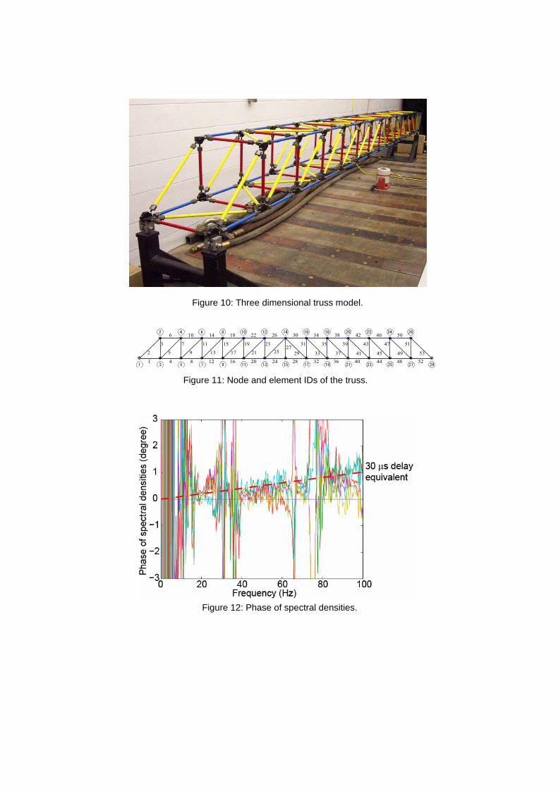
Figure 11: Node and element IDs of the truss.

1 4 8 12 16 20 24 28 32 36 40 44 48 52

6 10 14 18 22 26 30 34 38 42 46 50

3 7 11 15 19 2327

31 35 39 43 47 51

2 5 9 13 17 21 25 29 33 37 41 45 49 53

1

2 4 6 8

3 5 7 9

10 12 14 16

11 13 15 17 19 21 23 25 27 28

2618 20 22 24

Figure 10: Three dimensional truss model.

Figure 12: Phase of spectral densities.

Figure 14: Normalized accumulated stress from mass perturbation-based DCSmethod.

Figure 13: Cross spectral densities.

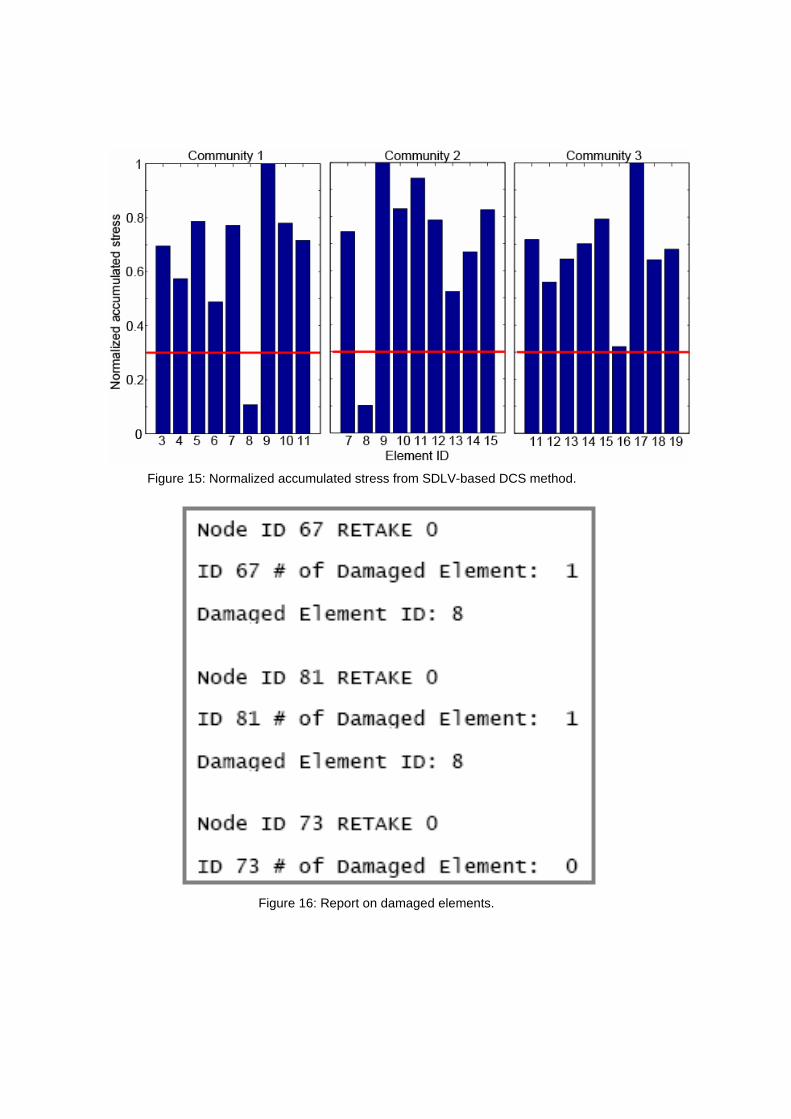
Figure 16: Report on damaged elements.

Figure 15: Normalized accumulated stress from SDLV-based DCS method.