Smart Quantum Statistical Imaging beyond the Abbe-Rayleigh Criterion

Narayan Bhusal,1, ∗ Mingyuan Hong,1, ∗ Nathaniel R. Miller,1, ∗ Mario A Quiroz-Juarez,2

Roberto de J. Leon-Montiel,3 Chenglong You,1, † and Omar S. Magana-Loaiza1

1Quantum Photonics Laboratory, Department of Physics & Astronomy,Louisiana State University, Baton Rouge, LA 70803, USA

2Departamento de Fısica, Universidad Autonoma Metropolitana Unidad Iztapalapa,San Rafael Atlixco 186, 09340 Ciudad Mexico, Mexico

3Instituto de Ciencias Nucleares, Universidad Nacional Autonoma de Mexico,Apartado Postal 70-543, 04510 Cd. Mx., Mexico

(Dated: October 12, 2021)

The manifestation of the wave nature of light through diffraction imposes limits on the resolutionof optical imaging. For over a century, the Abbe-Rayleigh criterion has been utilized to assess thespatial resolution limits of optical instruments. Recently, there has been an enormous impetus inovercoming the Abbe-Rayleigh resolution limit by projecting target light beams onto spatial modes.These conventional schemes for superresolution rely on a series of spatial projective measurementsto pick up phase information that is used to boost the spatial resolution of optical systems. Unfortu-nately, these schemes require a priori information regarding the coherence properties of “unknown”light beams. Furthermore, they require stringent alignment and centering conditions that cannotbe achieved in realistic scenarios. Here, we introduce a smart quantum camera for superresolvingimaging. This camera exploits the self-learning features of artificial intelligence to identify the sta-tistical fluctuations of unknown mixtures of light sources at each pixel. This is achieved through auniversal quantum model that enables the design of artificial neural networks for the identificationof quantum photon fluctuations. Our camera overcomes the inherent limitations of existing super-resolution schemes based on spatial mode projection. Thus, our work provides a new perspective inthe field of imaging with important implications for microscopy, remote sensing, and astronomy.

The spatial resolution of optical imaging systems isestablished by the diffraction of photons and the noiseassociated with their quantum fluctuations [1–5]. Forover a century, the Abbe-Rayleigh criterion has been usedto assess the diffraction-limited resolution of optical in-struments [3, 6]. At a more fundamental level, the ulti-mate resolution of optical instruments is established bythe laws of quantum physics through the Heisenberg un-certainty principle [7–9]. In classical optics, the Abbe-Rayleigh resolution criterion stipulates that an imag-ing system cannot resolve spatial features smaller thanλ/2NA. In this case, λ represents the wavelength of theillumination field, and NA describes numerical apertureof the optical instrument [1–3, 10]. Given the implica-tions that overcoming the Abbe-Rayleigh resolution limithas for multiple applications, such as, microscopy, re-mote sensing, and astronomy [3, 10–12], there has beenan enormous interest in improving the spatial resolutionof optical systems [13–15]. So far, optical superresolu-tion has been achieved through spatial decomposition ofeigenmodes [14, 16, 17]. These conventional schemes relyon spatial projective measurements to pick up phase in-formation that is used to boost spatial resolution of op-tical instruments [14, 18–22].

For almost a century, the importance of phase over am-plitude information has constituted established knowl-edge for optical engineers [3–5]. Recently, this idea hasbeen extensively investigated in the context of quan-tum metrology [5, 23–26]. More specifically, it has beendemonstrated that phase information can be used to sur-

pass the Abbe-Rayleigh resolution limit for the spatialidentification of light sources [13, 18–20, 27]. For exam-ple, phase information can be obtained through modedecomposition by using projective measurements or de-multiplexing of spatial modes [14, 17–20]. Naturally,these approaches require a priori information regardingthe coherence properties of the, in principle, “unknown”light sources [14, 15, 21, 22]. Furthermore, these tech-niques impose stringent requirements on the alignmentand centering conditions of imaging systems [14, 15, 17–22, 28, 29]. Despite these limitations, most, if not all,the current experimental protocols have relied on spatialprojections and demultiplexing in the Hermite-Gaussian,Laguerre-Gaussian, and parity basis [14, 17–22].

The quantum statistical fluctuations of photons es-tablish the nature of light sources [30–34]. As such,these fundamental properties are not affected by the spa-tial resolution of an optical instrument [34]. Here, wedemonstrate that measurements of the quantum statisti-cal properties of a light field enable imaging beyond theAbbe-Rayleigh resolution limit. This is performed by ex-ploiting the self-learning features of artificial intelligenceto identify the statistical fluctuations of photon mixtures[30]. More specifically, we demonstrate a smart quantumcamera with the capability to identify photon statisticsat each pixel. For this purpose, we introduce a universalquantum model that describes the photon statistics pro-duced by the scattering of an arbitrary number of lightsources. This model is used to design and train artifi-cial neural networks for the identification of light sources.

arX

iv:2

110.

0544

6v1

[qu

ant-

ph]

11

Oct

202

1

2

a b

FIG. 1. Conceptual illustration and schematic of our experimental setup to demonstrate superresolving imaging. The illustra-tion in a depicts a scenario where diffraction limits the resolution of an optical instrument for remote imaging. In our protocol,an artificial neural network enables the identification of the photon statistics that characterize the point sources that constitutea target object. In this case, the point sources emit either coherent or thermal photons. Remarkably, the neural networkis capable of identifying the corresponding photon fluctuations and their combinations, for example coherent-thermal (CT1,CT2), thermal-thermal (TT) and coherent-thermal-thermal (CTT). This capability allows us to boost the spatial resolutionof optical instruments beyond the Abbe-Rayleigh resolution limit. The experimental setup in b is designed to generate twoindependent thermal and one coherent light sources. The three sources are produced from a continuous-wave (CW) laser at633 nm. The CW laser beam is divided by two beam splitters (BS) to generate three spatial modes, two of which are thenpassed through rotating ground glass (RGG) disks to produce two independent thermal light beams. The three light sources,with different photon statistics, are attenuated using neutral density (ND) filters and then combined to mimic a remote objectsuch as the one shown in the inset of b. This setup enables us to generate multiple sources with tunable statistical properties.The generated target beam is then imaged onto a digital micro-mirror device (DMD) that we use to perform raster scanning.The photons reflected off the DMD are collected and measured by a single-photon detector. Our protocol is formalized byperforming photon-number-resolving detection [30]. The characteristic quantum fluctuations of each light source are identifiedby an artificial neural network. This information is then used to produce a high-resolution image of the object beyond thediffraction limit.

Remarkably, our scheme enables us to overcome inherentlimitations of existing superresolution protocols based onspatial mode projections and multiplexing [14, 17–22].

The conceptual schematic behind our experiment isdepicted in Fig. 1a. This camera utilizes an artificialneural network to identify the photon statistics of eachpoint source that constitutes a target object. The de-scription of the photon statistics produced by the scat-tering of an arbitrary number of light sources is achievedthrough a general model that relies on the quantum the-ory of optical coherence introduced by Sudarshan andGlauber [34–36]. We use this model to design and traina neural network capable of identifying light sources ateach pixel of our camera. This unique feature is achievedby performing photon-number-resolving detection [30].The sensitivity of this camera is limited by the photonfluctuations, as stipulated by the Heisenberg uncertaintyprinciple, and not by the Abbe-Rayleigh resolution limit[5, 34].

In general, realistic imaging instruments deal with thedetection of multiple light sources. These sources can beeither distinguishable or indistinguishable [3, 34]. Thecombination of indistinguishable sources can be repre-

sented by either coherent or incoherent superpositionsof light sources characterized by Poissonian (coherent)or super-Poissonionan (thermal) statistics [34]. In ourmodel, we first consider the indistinguishable detection ofN coherent and M thermal sources. For this purpose, wemake use of the P-function Pcoh(γ) = δ2(γ−αk) to modelthe contributions from the kth coherent source with thecorresponding complex amplitude αk [35, 36]. The to-tal complex amplitude associated to the superposition ofan arbitrary number of light sources is given by αtot =∑N

k=1 αk. In addition, the P-function for the lth thermalsource, with the corresponding mean photon numbers ml,is defined as Pth(γ) = (πml)

−1 exp (−|γ|2/ml). The to-tal number of photons attributed to the M number ofthermal sources is defined as mtot =

∑Ml=1 ml. These

quantities allow us to calculate the P-function for themultisource system as

Pth-coh(γ) =

∫· · ·∫PN+M (γ − γN+M−1)

×

[N+M−1∏

i=2

Pi(γi − γi−1)d2γi

]P1(γ1)d2γ1.

(1)

3

ωij(1)

Output LayerHidden LayerInput Layer

p (0)

p (1)

p (2)

p (20)

Ʃ

Ʃ

Ʃ

Ʃ

Ʃ

Ʃ

Ʃ

Ʃ

Ʃ

Class 4Coherent

Class 5Thermal

Class1Coherent-Thermal

Class 2Thermal-Thermal

Class 3Coherent-Thermal-Thermal

ωij(2)

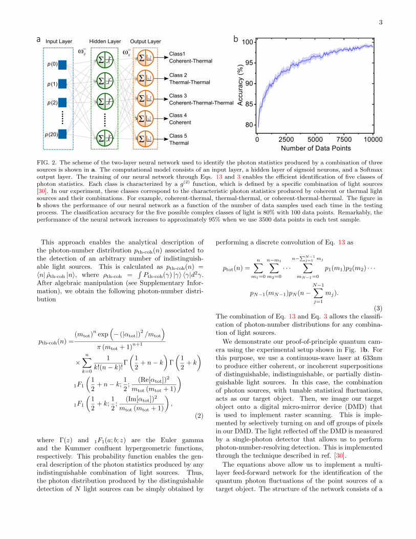
FIG. 2. The scheme of the two-layer neural network used to identify the photon statistics produced by a combination of threesources is shown in a. The computational model consists of an input layer, a hidden layer of sigmoid neurons, and a Softmaxoutput layer. The training of our neural network through Eqs. 13 and 3 enables the efficient identification of five classes ofphoton statistics. Each class is characterized by a g(2) function, which is defined by a specific combination of light sources[30]. In our experiment, these classes correspond to the characteristic photon statistics produced by coherent or thermal lightsources and their combinations. For example, coherent-thermal, thermal-thermal, or coherent-thermal-thermal. The figure inb shows the performance of our neural network as a function of the number of data samples used each time in the testingprocess. The classification accuracy for the five possible complex classes of light is 80% with 100 data points. Remarkably, theperformance of the neural network increases to approximately 95% when we use 3500 data points in each test sample.

This approach enables the analytical description ofthe photon-number distribution pth-coh(n) associated tothe detection of an arbitrary number of indistinguish-able light sources. This is calculated as pth-coh(n) =〈n| ρth-coh |n〉, where ρth-coh =

∫Pth-coh(γ) |γ〉 〈γ|d2γ.

After algebraic manipulation (see Supplementary Infor-mation), we obtain the following photon-number distri-bution

pth-coh(n) =(mtot)

nexp

(− (|αtot|)2 /mtot

)π (mtot + 1)

n+1

×n∑

k=0

1

k!(n− k)!Γ

(1

2+ n− k

)Γ

(1

2+ k

)

1F1

(1

2+ n− k;

1

2;

(Re[αtot])2

mtot (mtot + 1)

)1F1

(1

2+ k;

1

2;

(Im[αtot])2

mtot (mtot + 1)

),

(2)

where Γ(z) and 1F1(a; b; z) are the Euler gammaand the Kummer confluent hypergeometric functions,respectively. This probability function enables the gen-eral description of the photon statistics produced by anyindistinguishable combination of light sources. Thus,the photon distribution produced by the distinguishabledetection of N light sources can be simply obtained by

performing a discrete convolution of Eq. 13 as

ptot(n) =

n∑m1=0

n−m1∑m2=0

· · ·n−

∑N−1j=1 mj∑

mN−1=0

p1(m1)p2(m2) · · ·

pN−1(mN−1)pN (n−N−1∑j=1

mj).

(3)The combination of Eq. 13 and Eq. 3 allows the classifi-cation of photon-number distributions for any combina-tion of light sources.

We demonstrate our proof-of-principle quantum cam-era using the experimental setup shown in Fig. 1b. Forthis purpose, we use a continuous-wave laser at 633nmto produce either coherent, or incoherent superpositionsof distinguishable, indistinguishable, or partially distin-guishable light sources. In this case, the combinationof photon sources, with tunable statistical fluctuations,acts as our target object. Then, we image our targetobject onto a digital micro-mirror device (DMD) thatis used to implement raster scanning. This is imple-mented by selectively turning on and off groups of pixelsin our DMD. The light reflected off the DMD is measuredby a single-photon detector that allows us to performphoton-number-resolving detection. This is implementedthrough the technique described in ref. [30].

The equations above allow us to implement a multi-layer feed-forward network for the identification of thequantum photon fluctuations of the point sources of atarget object. The structure of the network consists of a

4

Data points=10 Data points=100

Data points=1000 Data points=10000

p(2)

p (0)p (1)

p(2)

p (0)p (1)

p(2)

p (0)p (1)

p(2)

p (0)p (1)

Coherent Thermal Thermal-ThermalCoherent-Thermal Coherent-Thermal-Thermal

a b

dc

Coherent Thermal Thermal-Thermal

Coherent-Thermal Coherent-Thermal-Thermal

Data points=10000Data points=1000

Data points=100Data points=10a b

c d

1

0.50

0.20.4

0.60

0.2

0.6

1

0.500

0.2

0

0.40

0.2

0.4

0.20

0.40.6

0.15

0.25

0

0.1

0.2

0.20

0.40.6

0.1

0.2

0.3

0.3

0.2

0.1

0

Data points=10 Data points=100

Data points=1000 Data points=10000

p(2)

p (0)p (1)

p(2)

p (0)p (1)

p(2)

p (0)p (1)

p(2)

p (0)p (1)

Coherent Thermal Thermal-ThermalCoherent-Thermal Coherent-Thermal-Thermal

a b

dcData points=10 Data points=100

Data points=1000 Data points=10000

p(2)

p (0)p (1)

p(2)

p (0)p (1)

p(2)

p (0)p (1)

p(2)

p (0)p (1)

Coherent Thermal Thermal-ThermalCoherent-Thermal Coherent-Thermal-Thermal

a b

dc

Data points=10 Data points=100

Data points=1000 Data points=10000

p(2)

p (0)p (1)

p(2)

p (0)p (1)

p(2)

p (0)p (1)

p(2)

p (0)p (1)

Coherent Thermal Thermal-ThermalCoherent-Thermal Coherent-Thermal-Thermal

a b

dcData points=10 Data points=100

Data points=1000 Data points=10000

p(2)

p (0)p (1)

p(2)

p (0)p (1)

p(2)

p (0)p (1)

p(2)

p (0)p (1)

Coherent Thermal Thermal-ThermalCoherent-Thermal Coherent-Thermal-Thermal

a b

dc

Data points=10 Data points=100

Data points=1000 Data points=10000

p(2)

p (0)p (1)

p(2)

p (0)p (1)

p(2)

p (0)p (1)

p(2)

p (0)p (1)

Coherent Thermal Thermal-ThermalCoherent-Thermal Coherent-Thermal-Thermal

a b

dc

Data points=10 Data points=100

Data points=1000 Data points=10000

p(2)

p (0)p (1)

p(2)

p (0)p (1)

p(2)

p (0)p (1)

p(2)

p (0)p (1)

Coherent Thermal Thermal-ThermalCoherent-Thermal Coherent-Thermal-Thermal

a b

dc

Data points=10 Data points=100

Data points=1000 Data points=10000

p(2)

p (0)p (1)

p(2)

p (0)p (1)

p(2)

p (0)p (1)

p(2)

p (0)p (1)

Coherent Thermal Thermal-ThermalCoherent-Thermal Coherent-Thermal-Thermal

a b

dc

Data points=10 Data points=100

Data points=1000 Data points=10000

p(2)

p (0)p (1)

p(2)

p (0)p (1)

p(2)

p (0)p (1)

p(2)

p (0)p (1)

Coherent Thermal Thermal-ThermalCoherent-Thermal Coherent-Thermal-Thermal

a b

dc

Data points=10 Data points=100

Data points=1000 Data points=10000

p(2)

p (0)p (1)

p(2)

p (0)p (1)

p(2)

p (0)p (1)

p(2)

p (0)p (1)

Coherent Thermal Thermal-ThermalCoherent-Thermal Coherent-Thermal-Thermal

a b

dc

Data points=10 Data points=100

Data points=1000 Data points=10000

p(2)

p (0)p (1)

p(2)

p (0)p (1)

p(2)

p (0)p (1)

p(2)

p (0)p (1)

Coherent Thermal Thermal-ThermalCoherent-Thermal Coherent-Thermal-Thermal

a b

dcData points=10 Data points=100

Data points=1000 Data points=10000

p(2)

p (0)p (1)

p(2)

p (0)p (1)

p(2)

p (0)p (1)

p(2)

p (0)p (1)

Coherent Thermal Thermal-ThermalCoherent-Thermal Coherent-Thermal-Thermal

a b

dc

Data points=10 Data points=100

Data points=1000 Data points=10000

p(2)

p (0)p (1)

p(2)

p (0)p (1)

p(2)

p (0)p (1)

p(2)

p (0)p (1)

Coherent Thermal Thermal-ThermalCoherent-Thermal Coherent-Thermal-Thermal

a b

dc

FIG. 3. Projection of the feature space on the plane definedby the probabilities p(0), p(1), and p(2). The red points corre-spond to the photon statistics for coherent light, and the bluepoints indicate the photon statistics for thermal light fields.Furthermore, the brown dots represent the photon statisticsproduced by the scattering of two thermal light sources, andthe black points show the photon statistics for a mixture ofphotons emitted by one coherent and one thermal source. Thecorresponding statistics for a mixture of one coherent and twothermal sources are indicated in green. As shown in a, thedistributions associated to the multiple sources obtained for10 data points are confined to a small region of the featurespace. A similar situation prevails in b for 100 data points. Asshown in panel c, the distributions produced with 1000 datapoints occupy different regions, although brown and blackpoints keep closely intertwined. Finally, the separated distri-butions obtained with 10000 data points in d enable efficientidentification of light sources.

group of interconnected neurons arranged in layers. Here,the information flows only in one direction, from inputto output [37, 38]. As indicated in Fig. 2a, our net-work comprises two layers, with ten sigmoid neurons inthe hidden layer (green neurons) and five softmax neu-rons in the output layer (orange neurons). In this case,the input features represent the probabilities of detectingn photons at a specific pixel, p(n), whereas the neuronsin the last layer correspond to the classes to be identi-fied. The input vector is then defined by twenty-one fea-tures corresponding to n=0,1,...,20. In our experiment,we define five classes that we label as: coherent-thermal(CT), thermal-thermal (TT), coherent-thermal-thermal(CTT), coherent (C), and thermal (T). If the brightness

of the experiment remains constant, these classes can bedirectly defined through the photon-number distributiondescribed by Eqs. 13 and 3. However, if the bright-ness of the sources is modified, the classes can be definedthrough the g(2) = 1 +

(⟨(∆n)2

⟩− 〈n〉

)/〈n〉2, which is

intensity-independent [30, 31]. The parameters in theg(2) function can also be calculated from Eqs. 13 and 3.It is important to mention that the output neurons pro-vide a probability distribution over the predicted classes[39, 40]. The training details of our neural networks canbe found in the Methods section.

We test the performance of our neural network throughthe classification of a complex mixture of photons pro-duced by the combination of one coherent with two ther-mal light sources. The accuracy of our trained neuralnetwork is reported in Fig. 2b. In our setup, the threepartially overlapping sources form five classes of lightwith different mean photon numbers and photon statis-tics. We exploit the functionality of our artificial neuralnetwork to identify the underlying quantum fluctuationsthat characterize each kind of light. We calculate theaccuracy as the ratio of true positive and true negativeto the total of input samples during the testing phase.Fig. 2b shows the overall accuracy as a function of thenumber of data points used to build the probability distri-butions for the identification of the multiple light sourcesusing a supervised neural network. The classification ac-curacy for the mixture of three light sources is 80% with100 photon-number-resolving measurements. The perfor-mance of the neural networks increases to approximately95% when we use 3500 data points to generate probabil-ity distributions.

The performance of our protocol for light identifica-tion can be understood through the distribution of lightsources in the probability space shown in Fig. 3. Herewe show the projection of the feature space on the planedefined by the probabilities p(0), p(1), and p(2) for dif-ferent number of data points. Each point is obtainedfrom an experimental probability distribution. As illus-trated in Fig. 3a, the distributions associated to themultiple sources obtained for 10 data points are con-fined to a small region of the feature space. This con-dition makes extremely hard the identification of lightsources with 10 sets of measurements. A similar situa-tion can be observed for the distribution in Fig. 3b thatwas generated using 100 data points. As shown in panelFig. 3c, the separations in the distributions producedwith 1000 data points occupy different regions, althoughbrown and black points keep closely intertwined. Theseconditions enable one to identify multiple light sources.Finally, the separated distributions obtained with 10000data points in Fig. 3d enable efficient identification oflight sources. These probability space diagrams explainthe performances reported in Fig. 2. An interesting fea-ture of Fig. 3 is the fact that the distributions in theprobability space are linearly separable.

5

0 1 2 3 4 5 6 7 8 9100

0.10.20.3

Probability Exp

Theory Exp Theory

Exp Theory

Exp Theory

Exp Theory

Exp Theory

0 1 2 3 4 5 6 7 8 9100

0.10.20.3

0 1 2 3 4 5 6 7 8 9100

0.10.20.3

0 1 2 3 4 5 6 7 8 9100

0.10.20.3

Probability

0 1 2 3 4 5 6 7 8 9100

0.10.20.3

0 1 2 3 4 5 6 7 8 9100

0.10.20.3

0 1 2 3 4 5 6 7 8 9100

0.10.20.3

Probability Exp

Theory Exp Theory

Exp Theory

Exp Theory

Exp Theory

Exp Theory

0 1 2 3 4 5 6 7 8 9100

0.10.20.3

0 1 2 3 4 5 6 7 8 9100

0.10.20.3

0 1 2 3 4 5 6 7 8 9100

0.10.20.3

Probability

0 1 2 3 4 5 6 7 8 9100

0.10.20.3

0 1 2 3 4 5 6 7 8 9100

0.10.20.3

Diffraction-limited Imaging Superresolving Imaging

0 1 2 3 4 5 6 7 8 9100

0.10.20.3

Probability Exp

Theory Exp Theory

Exp Theory

Exp Theory

Exp Theory

Exp Theory

0 1 2 3 4 5 6 7 8 9100

0.10.20.3

0 1 2 3 4 5 6 7 8 9100

0.10.20.3

0 1 2 3 4 5 6 7 8 9100

0.10.20.3

Probability

0 1 2 3 4 5 6 7 8 9100

0.10.20.3

0 1 2 3 4 5 6 7 8 9100

0.10.20.3

0 1 2 3 4 5 6 7 8 9100

0.10.20.3

Probability Exp

Theory Exp Theory

Exp Theory

Exp Theory

Exp Theory

Exp Theory

0 1 2 3 4 5 6 7 8 9100

0.10.20.3

0 1 2 3 4 5 6 7 8 9100

0.10.20.3

0 1 2 3 4 5 6 7 8 9100

0.10.20.3

Probability

0 1 2 3 4 5 6 7 8 9100

0.10.20.3

0 1 2 3 4 5 6 7 8 9100

0.10.20.3

Prob

abili

ty

Prob

abili

ty

Prob

abili

ty

Photon number

ExpTheory

0 1 2 3 4 5 6 7 8 9100

0.10.20.3

Probability Exp

Theory Exp Theory

Exp Theory

Exp Theory

Exp Theory

Exp Theory

0 1 2 3 4 5 6 7 8 9100

0.10.20.3

0 1 2 3 4 5 6 7 8 9100

0.10.20.3

0 1 2 3 4 5 6 7 8 9100

0.10.20.3

Probability

0 1 2 3 4 5 6 7 8 9100

0.10.20.3

0 1 2 3 4 5 6 7 8 9100

0.10.20.3

0 1 2 3 4 5 6 7 8 9100

0.10.20.3

Probability Exp

Theory Exp Theory

Exp Theory

Exp Theory

Exp Theory

Exp Theory

0 1 2 3 4 5 6 7 8 9100

0.10.20.3

0 1 2 3 4 5 6 7 8 9100

0.10.20.3

0 1 2 3 4 5 6 7 8 9100

0.10.20.3

Probability

0 1 2 3 4 5 6 7 8 9100

0.10.20.3

0 1 2 3 4 5 6 7 8 9100

0.10.20.3

ExpTheory

0 1 2 3 4 5 6 7 8 9100

0.10.20.3

Probability Exp

Theory Exp Theory

Exp Theory

Exp Theory

Exp Theory

Exp Theory

0 1 2 3 4 5 6 7 8 9100

0.10.20.3

0 1 2 3 4 5 6 7 8 9100

0.10.20.3

0 1 2 3 4 5 6 7 8 9100

0.10.20.3

Probability

0 1 2 3 4 5 6 7 8 9100

0.10.20.3

0 1 2 3 4 5 6 7 8 9100

0.10.20.3

0 1 2 3 4 5 6 7 8 9100

0.10.20.3

Probability Exp

Theory Exp Theory

Exp Theory

Exp Theory

Exp Theory

Exp Theory

0 1 2 3 4 5 6 7 8 9100

0.10.20.3

0 1 2 3 4 5 6 7 8 9100

0.10.20.3

0 1 2 3 4 5 6 7 8 9100

0.10.20.3

Probability

0 1 2 3 4 5 6 7 8 9100

0.10.20.3

0 1 2 3 4 5 6 7 8 9100

0.10.20.3

ExpTheory

0 1 2 3 4 5 6 7 8 9100

0.10.20.3

Probability Exp

Theory Exp Theory

Exp Theory

Exp Theory

Exp Theory

Exp Theory

0 1 2 3 4 5 6 7 8 9100

0.10.20.3

0 1 2 3 4 5 6 7 8 9100

0.10.20.3

0 1 2 3 4 5 6 7 8 9100

0.10.20.3

Probability

0 1 2 3 4 5 6 7 8 9100

0.10.20.3

0 1 2 3 4 5 6 7 8 9100

0.10.20.3

0 1 2 3 4 5 6 7 8 9100

0.10.20.3

Probability Exp

Theory Exp Theory

Exp Theory

Exp Theory

Exp Theory

Exp Theory

0 1 2 3 4 5 6 7 8 9100

0.10.20.3

0 1 2 3 4 5 6 7 8 9100

0.10.20.3

0 1 2 3 4 5 6 7 8 9100

0.10.20.3

Probability

0 1 2 3 4 5 6 7 8 9100

0.10.20.3

0 1 2 3 4 5 6 7 8 9100

0.10.20.3

Photon number

Photon number

Photon number

Pixel PositionPixel Position Pixel Position

Pixel Position

a b

e f

Normalized intensity

10

Prob

abili

ty ExpTheory

0 1 2 3 4 5 6 7 8 9100

0.10.20.3

Probability Exp

Theory Exp Theory

Exp Theory

Exp Theory

Exp Theory

Exp Theory

0 1 2 3 4 5 6 7 8 9100

0.10.20.3

0 1 2 3 4 5 6 7 8 9100

0.10.20.3

0 1 2 3 4 5 6 7 8 9100

0.10.20.3

Probability

0 1 2 3 4 5 6 7 8 9100

0.10.20.3

0 1 2 3 4 5 6 7 8 9100

0.10.20.3

0 1 2 3 4 5 6 7 8 9100

0.10.20.3

Probability Exp

Theory Exp Theory

Exp Theory

Exp Theory

Exp Theory

Exp Theory

0 1 2 3 4 5 6 7 8 9100

0.10.20.3

0 1 2 3 4 5 6 7 8 9100

0.10.20.3

0 1 2 3 4 5 6 7 8 9100

0.10.20.3

Probability

0 1 2 3 4 5 6 7 8 9100

0.10.20.3

0 1 2 3 4 5 6 7 8 9100

0.10.20.3

Diffraction-limited Imaging Superresolving Imaging

c d

𝑔(") =1.734 𝑔(") =1.301

𝑔(") =1.152

𝑔(") =1.4920 1 2 3 4 5 6 7 8 910

00.10.20.3

Probability Exp

Theory Exp Theory

Exp Theory

Exp Theory

Exp Theory

Exp Theory

0 1 2 3 4 5 6 7 8 9100

0.10.20.3

0 1 2 3 4 5 6 7 8 9100

0.10.20.3

0 1 2 3 4 5 6 7 8 9100

0.10.20.3

Probability

0 1 2 3 4 5 6 7 8 9100

0.10.20.3

0 1 2 3 4 5 6 7 8 9100

0.10.20.3

Prob

abili

ty

Photon number

ExpTheory

0 1 2 3 4 5 6 7 8 9100

0.10.20.3

Probability Exp

Theory Exp Theory

Exp Theory

Exp Theory

Exp Theory

Exp Theory

0 1 2 3 4 5 6 7 8 9100

0.10.20.3

0 1 2 3 4 5 6 7 8 9100

0.10.20.3

0 1 2 3 4 5 6 7 8 9100

0.10.20.3

Probability

0 1 2 3 4 5 6 7 8 9100

0.10.20.3

0 1 2 3 4 5 6 7 8 9100

0.10.20.3

0 1 2 3 4 5 6 7 8 9100

0.10.20.3

Probability Exp

Theory Exp Theory

Exp Theory

Exp Theory

Exp Theory

Exp Theory

0 1 2 3 4 5 6 7 8 9100

0.10.20.3

0 1 2 3 4 5 6 7 8 9100

0.10.20.3

0 1 2 3 4 5 6 7 8 9100

0.10.20.3

Probability

0 1 2 3 4 5 6 7 8 9100

0.10.20.3

0 1 2 3 4 5 6 7 8 9100

0.10.20.3

𝑔(") =1.166

𝑛$ = 3.24

𝑛$ = 1.48 𝑛$ = 2.93

𝑛$ = 3.42

𝑛$ = 1.48

0 1 2 3 4 5 6 7 8 9100

0.10.20.3

Probability Exp

Theory Exp Theory

Exp Theory

Exp Theory

Exp Theory

Exp Theory

0 1 2 3 4 5 6 7 8 9100

0.10.20.3

0 1 2 3 4 5 6 7 8 9100

0.10.20.3

0 1 2 3 4 5 6 7 8 9100

0.10.20.3

Probability

0 1 2 3 4 5 6 7 8 9100

0.10.20.3

0 1 2 3 4 5 6 7 8 9100

0.10.20.3

Prob

abili

ty Exp

0 1 2 3 4 5 6 7 8 9100

0.10.20.3

Probability Exp

Theory Exp Theory

Exp Theory

Exp Theory

Exp Theory

Exp Theory

0 1 2 3 4 5 6 7 8 9100

0.10.20.3

0 1 2 3 4 5 6 7 8 9100

0.10.20.3

0 1 2 3 4 5 6 7 8 9100

0.10.20.3

Probability

0 1 2 3 4 5 6 7 8 9100

0.10.20.3

0 1 2 3 4 5 6 7 8 9100

0.10.20.3

0 1 2 3 4 5 6 7 8 9100

0.10.20.3

Probability Exp

Theory Exp Theory

Exp Theory

Exp Theory

Exp Theory

Exp Theory

0 1 2 3 4 5 6 7 8 9100

0.10.20.3

0 1 2 3 4 5 6 7 8 9100

0.10.20.3

0 1 2 3 4 5 6 7 8 9100

0.10.20.3

Probability

0 1 2 3 4 5 6 7 8 9100

0.10.20.3

0 1 2 3 4 5 6 7 8 9100

0.10.20.3

Photon number

𝑔(") =1.401

𝑛$ = 1.89Theory

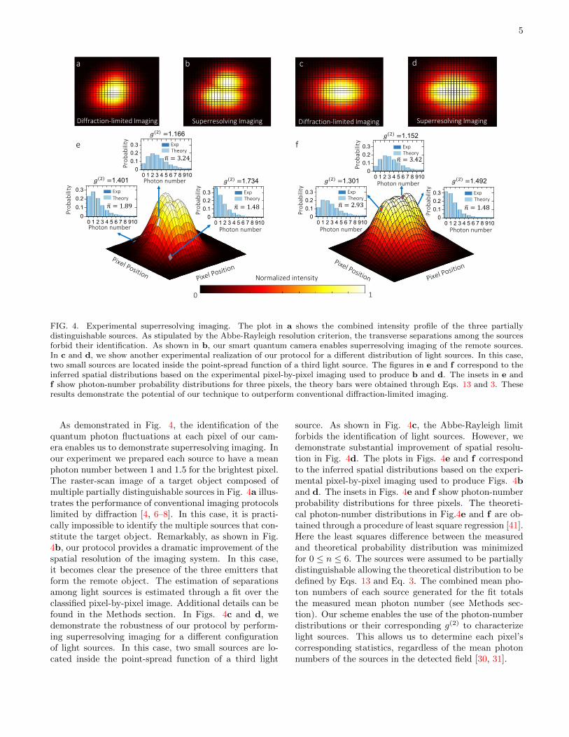
FIG. 4. Experimental superresolving imaging. The plot in a shows the combined intensity profile of the three partiallydistinguishable sources. As stipulated by the Abbe-Rayleigh resolution criterion, the transverse separations among the sourcesforbid their identification. As shown in b, our smart quantum camera enables superresolving imaging of the remote sources.In c and d, we show another experimental realization of our protocol for a different distribution of light sources. In this case,two small sources are located inside the point-spread function of a third light source. The figures in e and f correspond to theinferred spatial distributions based on the experimental pixel-by-pixel imaging used to produce b and d. The insets in e andf show photon-number probability distributions for three pixels, the theory bars were obtained through Eqs. 13 and 3. Theseresults demonstrate the potential of our technique to outperform conventional diffraction-limited imaging.

As demonstrated in Fig. 4, the identification of thequantum photon fluctuations at each pixel of our cam-era enables us to demonstrate superresolving imaging. Inour experiment we prepared each source to have a meanphoton number between 1 and 1.5 for the brightest pixel.The raster-scan image of a target object composed ofmultiple partially distinguishable sources in Fig. 4a illus-trates the performance of conventional imaging protocolslimited by diffraction [4, 6–8]. In this case, it is practi-cally impossible to identify the multiple sources that con-stitute the target object. Remarkably, as shown in Fig.4b, our protocol provides a dramatic improvement of thespatial resolution of the imaging system. In this case,it becomes clear the presence of the three emitters thatform the remote object. The estimation of separationsamong light sources is estimated through a fit over theclassified pixel-by-pixel image. Additional details can befound in the Methods section. In Figs. 4c and d, wedemonstrate the robustness of our protocol by perform-ing superresolving imaging for a different configurationof light sources. In this case, two small sources are lo-cated inside the point-spread function of a third light

source. As shown in Fig. 4c, the Abbe-Rayleigh limitforbids the identification of light sources. However, wedemonstrate substantial improvement of spatial resolu-tion in Fig. 4d. The plots in Figs. 4e and f correspondto the inferred spatial distributions based on the experi-mental pixel-by-pixel imaging used to produce Figs. 4band d. The insets in Figs. 4e and f show photon-numberprobability distributions for three pixels. The theoreti-cal photon-number distributions in Fig.4e and f are ob-tained through a procedure of least square regression [41].Here the least squares difference between the measuredand theoretical probability distribution was minimizedfor 0 ≤ n ≤ 6. The sources were assumed to be partiallydistinguishable allowing the theoretical distribution to bedefined by Eqs. 13 and Eq. 3. The combined mean pho-ton numbers of each source generated for the fit totalsthe measured mean photon number (see Methods sec-tion). Our scheme enables the use of the photon-numberdistributions or their corresponding g(2) to characterizelight sources. This allows us to determine each pixel’scorresponding statistics, regardless of the mean photonnumbers of the sources in the detected field [30, 31].

6

0 0.2 0.4 0.6 0.8 1

0

0.2

0.4

0.6

0.8

1 Monte Carlo Diffraction-Limited Imaging

Monte Carlo Superresolving Imaging

Experimental Superresolving Imaging

ai)

ii)iii)

b

i)

c

ii)

d

iii)

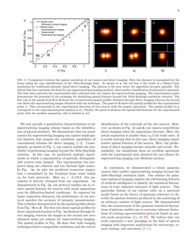
FIG. 5. Comparison between the spatial resolution of our camera and direct imaging. Here the distance is normalized by thebeam radius for easy identification of the Abbe-Rayleigh limit. As shown in a, the red line is the result of a Monte-Carlosimulation for traditional intensity based direct imaging. The plateau is the area where the algorithm becomes unstable. Thedotted blue line represents the limit for our supperresolving imaging method, where perfect classification of each pixel is assumed.The blue dots represent the experimental data collected with our camera for superresolving imaging. The experimental pointsdemonstrate the potential of our technique for identifying spatial features beyond the Abbe-Rayleigh resolution criterion. Thefirst row in the panels from b to d shows the reconstructed spatial profiles obtained through direct imaging whereas the secondrow shows the superresolving images obtained with our technique. The panel in b shows the spatial profiles for the experimentalpoint i). This corresponds to the experimental detection of two sources with the largest separation. The spatial profiles in ccorrespond to the experimental point labeled as ii). Finally, the panel in d shows the spatial distributions for the experimentalpoint with the smallest separation, this is labeled as iii).

We now provide a quantitative characterization of oursuperresolving imaging scheme based on the identifica-tion of photon statistics. We demonstrate that our smartcamera for superresolving imaging can capture small spa-tial features that surpass the resolution capabilities ofconventional schemes for direct imaging [1–5]. Conse-quently, as shown in Fig. 5, our camera enables the pos-sibility of performing imaging beyond the Abbe-Rayleighcriterion. In this case, we performed multiple experi-ments in which a superposition of partially distinguish-able sources were imaged. The superposition was pre-pared using one coherent and one thermal light source.In Fig. 5a, we plot the predicted transverse separa-tion s normalized by the Gaussian beam waist radiusw0 for both protocols. Here w0 = λ/πNA, this pa-rameter is directly obtained from our experiment. Asdemonstrated in Fig. 5a, our protocol enables one to re-solve spatial features for sources with small separationseven for diffraction-limited conditions. As expected forlarger separation distances, the performance of our pro-tocol matches the accuracy of intensity measurements.This is further demonstrated by the spatial profiles shownfrom Fig. 5b to d. The first row shows spatial profiles forthree experimental points in Fig. 5a obtained through di-rect imaging whereas the images in the second row wereobtained using our scheme for superresolving imaging.The spatial profiles in Fig. 5b show that both imagingtechniques lead to comparable resolutions and the correct

identification of the centroids of the two sources. How-ever, as shown in Fig. 5c and d, our camera outperformsdirect imaging when the separations decrease. Here, theactual separation is smaller than w0/2 for both cases. Itis worth noticing that in this case, direct imaging cannotresolve spatial features of the sources. Here, the predic-tions of direct imaging become unstable and erratic. Re-markably, our simulations show an excellent agreementwith the experimental data obtained for our scheme forsuperresolving imaging (see Methods section).

In conclusion, we demonstrated a robust quantumcamera that enables superresolving imaging beyond theAbbe-Rayleigh resolution limit. Our scheme for quan-tum statistical imaging exploits the self-learning featuresof artificial intelligence to identify the statistical fluctua-tions of truly unknown mixtures of light sources. Thisparticular feature of our scheme relies on a universalmodel based on the theory of quantum coherence to de-scribe the photon statistics produced by the scattering ofan arbitrary number of light sources. We demonstratedthat the measurement of the quantum statistical fluctua-tions of photons enables one to overcome inherent limita-tions of existing superresolution protocols based on spa-tial mode projections [14, 18–22]. We believe that ourwork represents a new paradigm in the field of opticalimaging with important implications for microscopy, re-mote sensing, and astronomy [5–11].

7

ACKNOWLEDGMENTS

N.B., M.H., C.Y., and O.S.M.L. acknowledge supportfrom the Army Research Office (ARO) under the grantno. W911NF-20-1-0194, the U.S. Department of Energy,Office of Basic Energy Sciences, Division of Materials Sci-ences and Engineering under Award DE-SC0021069, andthe Louisiana State University (LSU) Board of Super-visors for the LSU Leveraging Innovation for Technol-ogy Transfer (LIFT2) Grant under the grant no. LSU-2021-LIFT-004. N.M. thanks support from Departmentof Physics & Astronomy of Louisiana State University.R.J.L.M. thankfully acknowledges financial support byCONACyT under the project CB-2016-01/284372, andby DGAPA-UNAM, under the project UNAM-PAPIITIN102920.

COMPETING INTERESTS

The authors declare no competing interests.

DATA AVAILABILITY

The data sets generated and/or analyzed during thisstudy are available from the corresponding author or lastauthor on reasonable request.

METHODS

Training of NN

For the sake of simplicity, we split the functionalityof our neural network into two phases: the training andtesting phase. In the first phase, the training data isfed to the network multiple times to optimize the synap-tic weights through a scaled conjugate gradient back-propagation algorithm [42]. This optimization seeks tominimize the Kullback-Leibler divergence distance be-tween predicted and the real target classes [43, 44]. Atthis point, the training is stopped if the loss functiondoes not decrease within 1000 epochs [45]. In the testphase, we assess the performance of the algorithm by in-troducing an unknown set of data during the trainingprocess. For both phases, we prepare a data-set con-sisting of one thousand experimental measurements ofphoton statistics for each of the five classes. This processis formalized by considering different numbers of datapoints: 100, 500, ..., 9500, 10000. Following a standard-ized ratio for statistical learning, we divide our data intotraining (70%), validation (15%), and testing (15%) sets[46]. The networks were trained using the neural net-work toolbox in MATLAB, which runs on a computer

Intel Core i7–4710MQ CPU (@2.50GHz) with 32GB ofRAM.

Fittings

To determine the optimal fits for Fig. 4e and f we de-sign a search space based on Eqs. 13 and 3. To do so wefirst found the mean photon number of the input pixel,which will later be applied to constrain the search space.From here we allowed for the existence of up to threedistinguishable modes which will be combined accordingto Eq. 3. Each of the modes contains an indistinguish-able combination of up to one coherent and two thermalsources whose number distribution is given by Eq. 13.The total combination results in partially distinguishablecombination and provides the theoretical model for ourexperiment. From here our search space is

√∑n=0

(pexp(n)− pth(n|~n1,t, ~n2,t, ~nc))2,

where ~ni,t and ~nc are the mean photon numbers of thateach thermal or coherent source contributes to each dis-tinguishable mode respectively. The mean photon num-bers of each source must add up to the experimentalmean photon number, constraining the search. A linearsearch was then performed over the predicted mean pho-ton numbers and the minimum was returned, providingthe optimal fit.

Monte-Carlo Simulation of the Experiment

To demonstrate a consistent improvement over tradi-tional methods, we also simulated the experiment usingtwo beams, a thermal and a coherent, with Gaussianpoint spread functions over a 128×128 grid of pixels. Ateach pixel, the mean photon number for each source isprovided by the Gaussian point spread function, which isthen used to create the appropriate distinguishable prob-ability distribution as given in Eq. 3, creating a 128×128grid of photon number distributions. The associated classdata for these distributions will then be fitted using to aset of pre-labeled disks using a genetic algorithm. Thisrecreates our method in the limits of perfect classifica-tion. Each of these distributions is then used to simulatephoton-number resolving detection. This data is thenused to create a normalized intensity for the classical fit.We fit the image to a combination of Gaussian PSFs.This process is repeated ten times for each separation inorder to average out fluctuations in the fitting. Whencombining the results of the intensity fits they are firstdivided into two sets. One set has the majority of fitsreturn a single Gaussian, while the other returned two

8

Gaussian the majority of the time. The set identifiedas only containing a single Gaussian is then set at theAbbe-Rayleigh diffraction limit, while the remaining datais used in a linear fit. This causes the sharp transitionbetween the two sets of data.

∗ These authors contributed equally.† cyou2@lsu.edu

[1] E. Abbe, Beitrage zur theorie des mikroskops und dermikroskopischen wahrnehmung, Archiv fur mikroskopis-che Anatomie 9, 413 (1873).

[2] L. Rayleigh, Xxxi. investigations in optics, with specialreference to the spectroscope, The London, Edinburgh,and Dublin Philosophical Magazine and Journal of Sci-ence 8, 261 (1879).

[3] M. Born and E. Wolf, Principles of optics: electromag-netic theory of propagation, interference and diffractionof light (Elsevier, 2013).

[4] J. W. Goodman, Introduction to Fourier optics (Robertsand Company Publishers, 2005).

[5] O. S. Magana-Loaiza and R. W. Boyd, Quantum imagingand information, Rep. Prog. Phys. 82, 124401 (2019).

[6] R. Won, Eyes on super-resolution, Nat. Photonics 3, 368(2009).

[7] E. H. K. Stelzer, Beyond the diffraction limit?, Nature417, 806 (2002).

[8] M. I. Kolobov and C. Fabre, Quantum limits on opticalresolution, Phys. Rev. Lett. 85, 3789 (2000).

[9] E. H. K. Stelzer and S. Grill, The uncertainty principleapplied to estimate focal spot dimensions, Opt. Commun.173, 51 (2000).

[10] Beyond the diffraction limit, Nat. Photonics 3, 361(2009).

[11] S. Pirandola, B. R. Bardhan, T. Gehring, C. Weedbrook,and S. Lloyd, Advances in photonic quantum sensing,Nat. Photonics 12, 724 (2018).

[12] S. W. Hell, S. J. Sahl, M. Bates, X. Zhuang, R. Heintz-mann, M. J. Booth, J. Bewersdorf, G. Shtengel, H. Hess,P. Tinnefeld, A. Honigmann, S. Jakobs, I. Testa,L. Cognet, B. Lounis, H. Ewers, S. J. Davis, C. Eggeling,D. Klenerman, K. I. Willig, G. Vicidomini, M. Castello,A. Diaspro, and T. Cordes, The 2015 super-resolution mi-croscopy roadmap, J. Phys. D: Appl. Phys. 48, 443001(2015).

[13] M. Tsang, Quantum imaging beyond the diffraction limitby optical centroid measurements, Phys. Rev. Lett. 102,253601 (2009).

[14] M. Tsang, R. Nair, and X.-M. Lu, Quantum theory ofsuperresolution for two incoherent optical point sources,Phys. Rev. X 6, 031033 (2016).

[15] S. W. Hell and J. Wichmann, Breaking the diffrac-tion resolution limit by stimulated emission: stimulated-emission-depletion fluorescence microscopy, Opt. Lett.19, 780 (1994).

[16] M. Paur, B. Stoklasa, J. Grover, A. Krzic, L. L. Sanchez-Soto, Z. Hradil, and J. Rehacek, Tempering Rayleigh’scurse with PSF shaping, Optica 5, 1177 (2018).

[17] F. Tamburini, G. Anzolin, G. Umbriaco, A. Bianchini,and C. Barbieri, Overcoming the Rayleigh criterion limitwith optical vortices, Phys. Rev. Lett. 97, 163903 (2006).

[18] W.-K. Tham, H. Ferretti, and A. M. Steinberg, Beat-ing rayleigh’s curse by imaging using phase information,Phys. Rev. Lett. 118, 070801 (2017).

[19] Y. Zhou, J. Yang, J. D. Hassett, S. M. H. Rafsanjani,M. Mirhosseini, A. N. Vamivakas, A. N. Jordan, Z. Shi,and R. W. Boyd, Quantum-limited estimation of the ax-ial separation of two incoherent point sources, Optica 6,534 (2019).

[20] P. Boucher, C. Fabre, G. Labroille, and N. Treps, Spa-tial optical mode demultiplexing as a practical tool foroptimal transverse distance estimation, Optica 7, 1621(2020).

[21] W. Larson and B. E. A. Saleh, Resurgence of Rayleigh’scurse in the presence of partial coherence, Optica 5, 1382(2018).

[22] K. Liang, S. A. Wadood, and A. N. Vamivakas, Coher-ence effects on estimating two-point separation, Optica8, 243 (2021).

[23] A. N. Boto, P. Kok, D. S. Abrams, S. L. Braunstein, C. P.Williams, and J. P. Dowling, Quantum interferometricoptical lithography: Exploiting entanglement to beat thediffraction limit, Phys. Rev. Lett. 85, 2733 (2000).

[24] Z. S. Tang, K. Durak, and A. Ling, Fault-tolerant andfinite-error localization for point emitters within thediffraction limit, Opt. Express 24, 22004 (2016).

[25] M. Parniak, S. Borowka, K. Boroszko, W. Wasilewski,K. Banaszek, and R. Demkowicz-Dobrzanski, Beating theRayleigh limit using two-photon interference, Phys. Rev.Lett. 121, 250503 (2018).

[26] C. You, M. Hong, P. Bierhorst, A. E. Lita, S. Glancy,S. Kolthammer, E. Knill, S. W. Nam, R. P. Mirin, O. S.Magana-Loaiza, and T. Gerrits, Scalable multiphotonquantum metrology with neither pre- nor post-selectedmeasurements (2021), arXiv:2011.02454 [quant-ph].

[27] V. Giovannetti, S. Lloyd, L. Maccone, and J. H. Shapiro,Sub-Rayleigh-diffraction-bound quantum imaging, Phys.Rev. A 79, 013827 (2009).

[28] O. S. Magana-Loaiza, M. Mirhosseini, R. M.Cross, S. M. H. Rafsanjani, and R. W. Boyd,Hanbury brown and twiss interferometry withtwisted light, Sci. Adv. 2, e1501143 (2016),https://www.science.org/doi/pdf/10.1126/sciadv.1501143.

[29] Z. Yang, O. S. Magana-Loaiza, M. Mirhosseini, Y. Zhou,B. Gao, L. Gao, S. M. H. Rafsanjani, G.-L. Long, andR. W. Boyd, Digital spiral object identification usingrandom light, Light: Science & Applications 6, e17013(2017).

[30] C. You, M. A. Quiroz-Juarez, A. Lambert, N. Bhusal,C. Dong, A. Perez-Leija, A. Javaid, R. de J. Leon-Montiel, and O. S. Magana-Loaiza, Identification of lightsources using machine learning, Appl. Phys. Rev. 7,021404 (2020).

[31] C. You, M. Hong, N. Bhusal, J. Chen, M. A. Quiroz-Juarez, J. Fabre, F. Mostafavi, L. Guo, I. De Leon,R. de J. Leon-Montiel, and O. S. Magana-Loaiza, Obser-vation of the modification of quantum statistics of plas-monic systems, Nat Commun 12, 5161 (2021).

[32] L. Mandel, Sub-poissonian photon statistics in resonancefluorescence, Opt. Lett. 4, 205 (1979).

[33] O. S. Magana-Loaiza, R. de J. Leon-Montiel, A. Perez-Leija, A. B. U’Ren, C. You, K. Busch, A. E. Lita, S. W.Nam, R. P. Mirin, and T. Gerrits, Multiphoton quantum-state engineering using conditional measurements, npjQuantum Inf. 5, 80 (2019).

9

[34] C. Gerry, P. Knight, and P. L. Knight, Introductory quan-tum optics (Cambridge university press, 2005).

[35] E. C. G. Sudarshan, Equivalence of semiclassical andquantum mechanical descriptions of statistical lightbeams, Phys. Rev. Lett. 10, 277 (1963).

[36] R. J. Glauber, The quantum theory of optical coherence,Phys. Rev. 130, 2529 (1963).

[37] D. Svozil, V. Kvasnicka, and J. Pospichal, Introduction tomulti-layer feed-forward neural networks, Chemom. In-tell. Lab. Syst. 39, 43 (1997).

[38] N. Bhusal, S. Lohani, C. You, M. Hong, J. Fabre, P. Zhao,E. M. Knutson, R. T. Glasser, and O. S. Magana-Loaiza,Spatial mode correction of single photons using machinelearning, Adv. Quantum Technol. 4, 2000103 (2021).

[39] I. Goodfellow, Y. Bengio, A. Courville, and Y. Bengio,Deep learning, Vol. 1 (MIT press Cambridge, 2016).

[40] C. M. Bishop, Pattern recognition and machine learning(springer, 2006).

[41] L. Massaron and A. Boschetti, Regression Analysis withPython (Packt Publishing Ltd, 2016).

[42] M. F. Møller, A scaled conjugate gradient algorithm forfast supervised learning, Neural Networks 6, 525 (1993).

[43] S. Kullback and R. A. Leibler, On information and suf-ficiency, The Annals of Mathematical Statistics 22, 79(1951).

[44] S. Kullback, Information theory and statistics (CourierCorporation, 1997).

[45] L. Prechelt, Early stopping - but when?, in Neural Net-works: Tricks of the Trade, edited by G. B. Orr and K.-R.Muller (Springer Berlin Heidelberg, Berlin, Heidelberg,1998) pp. 55–69.

[46] P. S. Crowther and R. J. Cox, A method for optimal divi-sion of data sets for use in neural networks, in Knowledge-Based Intelligent Information and Engineering Systems,edited by R. Khosla, R. J. Howlett, and L. C. Jain(Springer Berlin Heidelberg, Berlin, Heidelberg, 2005)pp. 1–7.

SUPPLEMENTARY MATERIAL: DERIVATION OF THE MANY-SOURCE PHOTON-NUMBERDISTRIBUTION

Let us start by considering the indistinguishable detection of N coherent and M thermal independent sources. Toobtain the combined photon distribution, we make use of the Glauber-Sudarshan theory of coherence [35, 36]. Thus,we start by writing the P-functions associated to the fields produced by the indistinguishable coherent and thermalsources, that is, we write

Pcoh (α) =

∫P cohN

(α− α

N−1

)P cohN−1

(α

N−1− α

N−2

)· · ·P coh

2 (α2 − α1)P coh1 (α1) d2α

N−1d2α

N−2· · · d2α2d

2α1 , (4)

Pth (α) =

∫P thM

(α− α

M−1

)P thM−1

(α

M−1− α

M−2

)· · ·P th

2 (α2 − α1)P th1 (α1) d2α

M−1d2α

M−2· · · d2α2d

2α1 , (5)

with Pcoh (α) and Pth (α) standing for the P-functions of the combined N -coherent and M -thermal sources, respec-tively. In both equations, α stands for the complex amplitude as defined for coherent states |α〉, and the individual-source P-functions are defined as

P cohk (α) = δ2 (α− αk) , (6)

P thl (α) =

1

πmlexp

(− |α|2 /ml

), (7)

where P cohk (α) corresponds to the P-function of kth coherent source, with mean photon number nk = |αk|2, and

P thl (α) describes the lth thermal source, with mean photon number ml.

Now, by substituting Eq. (6) into Eq. (4), and Eq. (7) into Eq. (5), we obtain

Pcoh (α) = δ2

(α−

N∑k=1

αk

), (8)

Pth (α) =1

π∑M

l=1 ml

exp

(− |α|2∑M

l=1 ml

). (9)

We can finally combine the thermal and coherent sources by writing

Pth-coh (α) =

∫Pth (α− α′)Pcoh (α′) d2α′. (10)

10

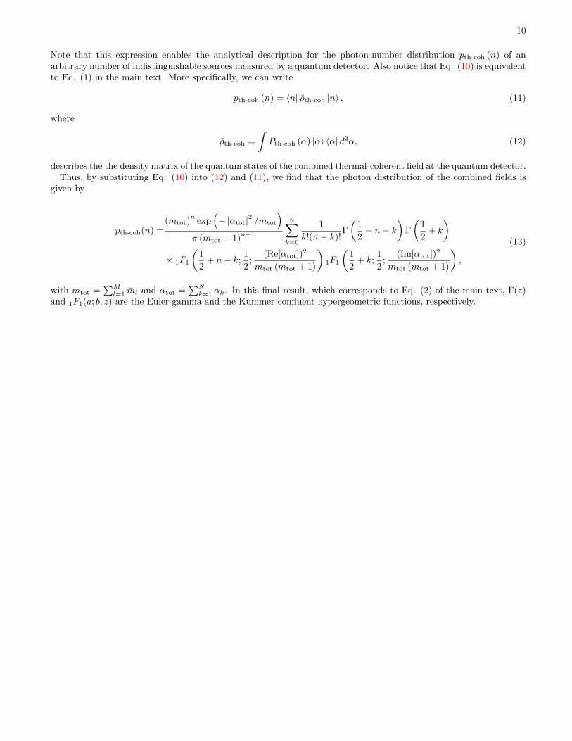
Note that this expression enables the analytical description for the photon-number distribution pth-coh (n) of anarbitrary number of indistinguishable sources measured by a quantum detector. Also notice that Eq. (10) is equivalentto Eq. (1) in the main text. More specifically, we can write

pth-coh (n) = 〈n| ρth-coh |n〉 , (11)

where

ρth-coh =

∫Pth-coh (α) |α〉 〈α| d2α, (12)

describes the the density matrix of the quantum states of the combined thermal-coherent field at the quantum detector.Thus, by substituting Eq. (10) into (12) and (11), we find that the photon distribution of the combined fields is

given by

pth-coh(n) =(mtot)

nexp

(− |αtot|2 /mtot

)π (mtot + 1)

n+1

n∑k=0

1

k!(n− k)!Γ

(1

2+ n− k

)Γ

(1

2+ k

)× 1F1

(1

2+ n− k;

1

2;

(Re[αtot])2

mtot (mtot + 1)

)1F1

(1

2+ k;

1

2;

(Im[αtot])2

mtot (mtot + 1)

),

(13)

with mtot =∑M

l=1 ml and αtot =∑N

k=1 αk. In this final result, which corresponds to Eq. (2) of the main text, Γ(z)and 1F1(a; b; z) are the Euler gamma and the Kummer confluent hypergeometric functions, respectively.