Smart Proxy Modeling of a Fractured Reservoir Model for ...

Original Paper

Smart Proxy Modeling of a Fractured Reservoir Modelfor Production Optimization: Implementationof Metaheuristic Algorithm and Probabilistic Application

Cuthbert Shang Wui Ng,1,3 Ashkan Jahanbani Ghahfarokhi,1 Menad Nait Amar,2

and Ole Torsæter1

Received 23 August 2020; accepted 13 February 2021Published online: 8 March 2021

Numerical reservoir simulation has been recognized as one of the most frequently used aidsin reservoir management. Despite having high calculability performance, it presents an acuteshortcoming, namely the long computational time induced by the complexities of reservoirmodels. This situation applies aptly in the modeling of fractured reservoirs because thesereservoirs are strongly heterogeneous. Therefore, the domains of artificial intelligence andmachine learning (ML) were used to alleviate this computational challenge by creating anew class of reservoir modeling, namely smart proxy modeling (SPM). SPM is a ML ap-proach that requires a spatio-temporal database extracted from the numerical simulation tobe built. In this study, we demonstrate the procedures of SPM based on a synthetic fracturedreservoir model, which is a representation of dual-porosity dual-permeability model. Theapplied ML technique for SPM is artificial neural network. We then present the applicationof the smart proxies in production optimization to illustrate its practicality. Apart fromapplying the backpropagation algorithms, we implemented particle swarm optimization(PSO), which is one of the metaheuristic algorithms, to build the SPM. We also propose anadditional procedure in SPM by integrating the probabilistic application to examine theoverall performance of the smart proxies. In this work, we inferred that the PSO had ahigher chance to improve the reliability of smart proxies with excellent training results andpredictive performance compared with the considered backpropagation approaches.

KEY WORDS: Reservoir simulation, Dual-porosity dual-permeability, Smart proxy modeling, Back-propagation algorithms, Particle swarm optimization.

INTRODUCTION

Hydrocarbons are among the primary sourcesof energy in today�s world. This is proven by a sta-tistical review conducted by British Petroleum

(2020), which found that, in 2019, oil contributed tothe largest share of the world primary energy ofabout 33.1%, whereas natural gas had the thirdlargest share of 24.2%. Hence, they play a pivotalrole in quenching the high demand of world energyconsumption and such demand will be likely in anupward trend due to the increasing global popula-tion (Gerald et al. 2014; International EnergyAgency 2018). In addition, the importance ofhydrocarbons is reflected by the significant influenceof their price on many other major economic do-

1Department of Geoscience and Petroleum, Norwegian Univer-

sity of Science and Technology, Trondheim, Norway.2Departement Etudes Thermodynamiques, Division

Laboratoires, Sonatrach, Boumerdes, Algeria.3To whom correspondence should be addressed; e-mail:

[email protected]

2431

1520-7439/21/0600-2431/0 � 2021 The Author(s)

Natural Resources Research, Vol. 30, No. 3, June 2021 (� 2021)

https://doi.org/10.1007/s11053-021-09844-2

http://crossmark.crossref.org/dialog/?doi=10.1007/s11053-021-09844-2&domain=pdf

mains (Lescaroux and Mignon 2009). This is illus-trated clearly by the phenomenon of how manyother industries have been affected by the fluctua-tion of oil price (Lescaroux and Mignon 2009).Therefore, it is essential to have a sustainablehydrocarbon production not only to fulfill the de-mand for energy consumption, but also to maintainthe global economic growth. With respect to this,carbonate reservoirs are one of the main sources ofhydrocarbons. These reservoirs make up approxi-mately 60% of the global oil reserves and about 40%of the global gas reserves (Schlumberger 2020b).Most of these reservoirs are naturally fractured, andhence, accurate modeling of fluid flow in thesereservoirs is one of the most critical steps to ensurethe sustainable production of hydrocarbons.

In general, modeling of fluid flow in porousmedia can be perceived as a numerical reservoirsimulation. Reservoir simulation is one of the mostfrequently used tools in reservoir management,which is the application of technological, labor, andfinancial resources to maximize the economic per-formance and the hydrocarbon recovery of a reser-voir (Wiggins and Startzman 1990). This is because ithas been implemented extensively to help predictthe performance of a reservoir as well as to provideuseful information for uncertainty analysis or anyoptimization task that includes enhanced oil recov-ery, hydraulic fracturing, and so forth. However, oneof the challenges of accurate modeling of fracturedreservoirs stems from a lack of underlying theory orprinciple to describe the behavior of fluid flow inthese reservoirs. To mitigate this challenge, Bar-renblatt (1960) established a theory pertaining tofluid flow in fractured porous media. Based on thistheory, Warren and Root (1963) developed the dual-porosity method, which has been one of the mostfundamental tools in simulating a fractured reser-voir. However, this conventional model does notsufficiently capture the realistic behavior of fluidflow as fluid is assumed to move only through frac-tures, whereas the matrix blocks only supply fluid tofractures. Hence, this model was enhanced to thedual-porosity dual-permeability (DPDP) model, inwhich the transport of fluid between matrix blocks isconsidered (Uleberg and Kleppe 1996). The detailsregarding this model are explained further below.

Having developed the DPDP model impliesthat fractured reservoirs can be simulated numeri-cally. Nonetheless, another challenge in terms of

computational effort arises as the complexity ofsimulated fractured reservoirs increases (includingas much details as possible to ‘‘describe realistically’’a reservoir). Therefore, reservoir managementmight not be sufficiently efficient to keep up withsustainable hydrocarbon production. Fortunately, intoday�s world of digitalization, methods of artificialintelligence and machine learning (AI&ML) havecome to the rescue. In this context, Ertekin and Sun(2019) provided a very comprehensive review on theimplementation of AI&ML methods in the field ofreservoir engineering. They also proposed the use ofhand-shaking protocol that would combine theadvantages of both traditional and intelligent reser-voir modeling to develop more powerful computa-tional protocols. With this, the great potential andextensive utilization of AI&ML-based methods havealso been demonstrated further in many technicaldomains of the petroleum industry (Mohaghegh2000a, b, c; Parada and Ertekin 2012; Nait Amar andJahanbani Ghahfarokhi 2020; Nait Amar et al.2020). Moreover, with the help of AI&ML, Moha-ghegh (2011) has coined a new class of reservoirmodeling, namely smart proxy modeling (SPM).Fundamentally, SPM is the development of an arti-ficial neural network (ANN) that receives both inputand output data from a reservoir simulation modeland undergoes a training phase. After the ANN hasbeen trained to recognize the pattern induced by thedata (relationship between input and output), it canyield the estimated result that matches with thatproduced by the reservoir model within a few sec-onds or minutes. Therefore, this ANN is termed‘‘smart proxy.’’ Regarding this, the word ‘‘smart’’reveals the ability to learn and capture the under-lying physical behavior of a simulated reservoirmodel through pattern recognition and the word‘‘proxy’’ denotes to act on behalf of the originalmodel (Mohaghegh 2017, 2018).

For the past decade, SPM has been consideredas a technological breakthrough in the petroleumindustry as it has not only reduced the reservoirsimulation time significantly, but it also provided theresults within an acceptable range of accuracy. Thesuccessful application of smart proxies has beendemonstrated in many literatures of the oil and gasindustry. Mohaghegh et al. (2006) developed surro-gate reservoir model (the initial nomenclature ofSPM), which was an accurate representation of asophisticated full-field reservoir model, and used it

2432 Ng, Ghahfarokhi, Amar, and Torsaeter

for uncertainty analysis. With this breakthrough,these surrogate models were implemented on dif-ferent real fields in Saudi Arabia for geologicaluncertainty analysis (Mohaghegh et al. 2012a, c).Mohaghegh et al. (2012b, 2015) then reformulatedthe concept of SPM by categorizing it as grid-basedand well-based. As the nomenclatures imply, grid-based SPM is done for the analysis of numericalmodel at grid block level, whereas well-based SPMis for the analysis at well level. Grid-based SPM hasbeen applied in several real-life CO2 sequestrationprojects (Mohaghegh et al. 2012b), whereas well-based SPM has been implemented for optimizationof production scheduling of a real field in UnitedArab Emirates (Mohaghegh et al. 2015). Besides,the application of SPM was then extended graduallyto other domains, such as history matching and en-hanced oil recovery (EOR). He et al. (2016) coupledthe use of SPM with differential evolution (DE) toperform automatic history matching. Alenezi andMohaghegh (2016) also built a SPM that reproducedand forecasted the dynamic properties of a reservoirthat has been water-flooded. Moreover, Mohaghegh(2018) discussed the utilization of SPM under thecontext of CO2-EOR as a storage mechanism. Fur-thermore, Parada and Ertekin (2012) applied SPMto establish successfully a new screening tool forfour different improved oil recovery (IOR) meth-ods, including waterflooding, miscible injection ofCO2 and N2, and injection of steam. Therefore,these literatures do not only show the high applica-bility of SPM in oil and gas industry, but they alsohighlight its potential for further enhancement.

Nevertheless, SPM still has few disadvantages.One of them is that a smart proxy built can only beapplied to predict what the simulated reservoirmight estimate only if the physics assumed in thenumerical simulation is not changed. For instance, ifa smart proxy is developed on a reservoir modelwith reservoir pressure of 4000 psia,1 then it cannotbe applied to perform any estimation of parameterswhen the reservoir pressure is not 4000 psia. Tohandle this problem, another smart proxy needs tobe established. In addition to this, the spatio-tem-poral database is considered as the backbone of theSPM as it is the main component used to train theANN model. Thus, if another smart proxy is built (as

previously mentioned), then the database needs tobe prepared again. Despite having such inconve-nience, the time spent on preparation of this data-base is still much less than the time spent bynumerical simulation. Pertaining to this, the prepa-ration of a spatio-temporal database might takeabout few hours (or for few minutes with the help ofcommercial software). However, for a sophisticatedreservoir simulation model, the computation mighttake a few days. It is important to understand thatsmart proxy is another example of data-drivenmodel as it is developed by analyzing the collecteddata (Alenezi and Mohaghegh 2016, 2017). Hence,careful attention is required when a spatio-temporaldatabase is created. If incorrect data are provided tothe smart proxy, it will ‘‘learn wrongly’’ and produceunsatisfactory results. This complies with the shortphrase that goes ‘‘garbage in and garbage out.’’

Although there are many literatures explainingthe theoretical basis of SPM, it is still treated as‘‘black-box’’ as commercial software is mostly usedto build a smart proxy. Thus, in this work, one of theobjectives was to provide a more vivid illustration ofhow SPM can be performed based on a syntheticreservoir model. Besides, we present another alter-native of training algorithm apart from the back-propagation algorithm that is mostly used in SPM.More intriguingly, we include a probabilistic appli-cation to evaluate further the overall performance ofthe developed SPMs. We opine that this integrationin SPM is insightful as it helps to better reflect theperformance of the proxy models. After this intro-duction, we discuss briefly the mathematical con-cepts of the DPDP model and how ANN operates.Three different algorithms, which are two examplesof backpropagation algorithms, namely stochasticgradient descent (SGD) and adaptive moment esti-mation (Adam) algorithms, and particle swarmoptimization (PSO), were implemented as thelearning algorithm to train the ANN. Hence, thefundamentals of these algorithms are discussed next.Then, we explicate the background of the reservoirmodel simulated based on the DPDP method andthe problem setting of the production optimizationcase. We also explain how the respective SPM isdeveloped upon it and used in production opti-mization. Then, the results and discussion will fol-low. Prior to proceeding to conclusions, we alsoprovide another case study, which considers aheterogeneous fractured reservoir model, to furthershow the robustness of the methodology discussed inthis paper.1 1 psia = 6894.75728 Pa.

2433Smart Proxy Modeling of a Fractured Reservoir Model for Production Optimization

METHODOLOGY

Fundamentals of DPDP Model

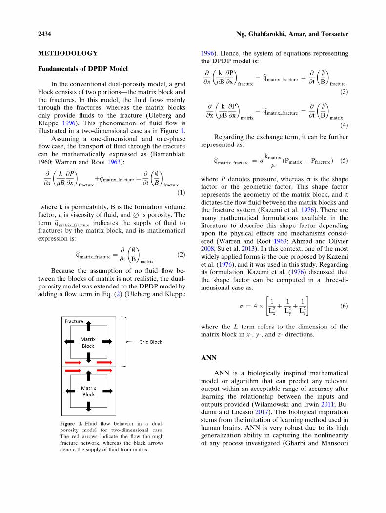
In the conventional dual-porosity model, a gridblock consists of two portions—the matrix block andthe fractures. In this model, the fluid flows mainlythrough the fractures, whereas the matrix blocksonly provide fluids to the fracture (Uleberg andKleppe 1996). This phenomenon of fluid flow isillustrated in a two-dimensional case as in Figure 1.

Assuming a one-dimensional and one-phaseflow case, the transport of fluid through the fracturecan be mathematically expressed as (Barrenblatt1960; Warren and Root 1963):

@

@x

k

lB@P

@x

� �fracture

þqmatrix fracture ¼@

@t

;B

� �fracture

ð1Þ

where k is permeability, B is the formation volumefactor, l is viscosity of fluid, and £ is porosity. Theterm bqmatrix fracture indicates the supply of fluid tofractures by the matrix block, and its mathematicalexpression is:

� bqmatrix fracture ¼@

@t

;B

� �matrix

ð2Þ

Because the assumption of no fluid flow be-tween the blocks of matrix is not realistic, the dual-porosity model was extended to the DPDP model byadding a flow term in Eq. (2) (Uleberg and Kleppe

1996). Hence, the system of equations representingthe DPDP model is:

@

@x

k

lB@P

@x

� �fracture

þ bqmatrix fracture ¼ @

@t

;B

� �fracture

ð3Þ

@

@x

k

lB@P

@x

� �matrix

� bqmatrix fracture ¼ @

@t

;B

� �matrix

ð4ÞRegarding the exchange term, it can be further

represented as:

� bqmatrix fracture ¼ rkmatrix

lPmatrix � Pfractureð Þ ð5Þ

where P denotes pressure, whereas r is the shapefactor or the geometric factor. This shape factorrepresents the geometry of the matrix block, and itdictates the flow fluid between the matrix blocks andthe fracture system (Kazemi et al. 1976). There aremany mathematical formulations available in theliterature to describe this shape factor dependingupon the physical effects and mechanisms consid-ered (Warren and Root 1963; Ahmad and Olivier2008; Su et al. 2013). In this context, one of the mostwidely applied forms is the one proposed by Kazemiet al. (1976), and it was used in this study. Regardingits formulation, Kazemi et al. (1976) discussed thatthe shape factor can be computed in a three-di-mensional case as:

r ¼ 4� 1

L2x

þ 1

L2y

þ 1

L2z

" #ð6Þ

where the L term refers to the dimension of thematrix block in x-, y-, and z- directions.

ANN

ANN is a biologically inspired mathematicalmodel or algorithm that can predict any relevantoutput within an acceptable range of accuracy afterlearning the relationship between the inputs andoutputs provided (Wilamowski and Irwin 2011; Bu-duma and Locasio 2017). This biological inspirationstems from the imitation of learning method used inhuman brains. ANN is very robust due to its highgeneralization ability in capturing the nonlinearityof any process investigated (Gharbi and Mansoori

Figure 1. Fluid flow behavior in a dual-

porosity model for two-dimensional case.

The red arrows indicate the flow thorough

fracture network, whereas the black arrows

denote the supply of fluid from matrix.


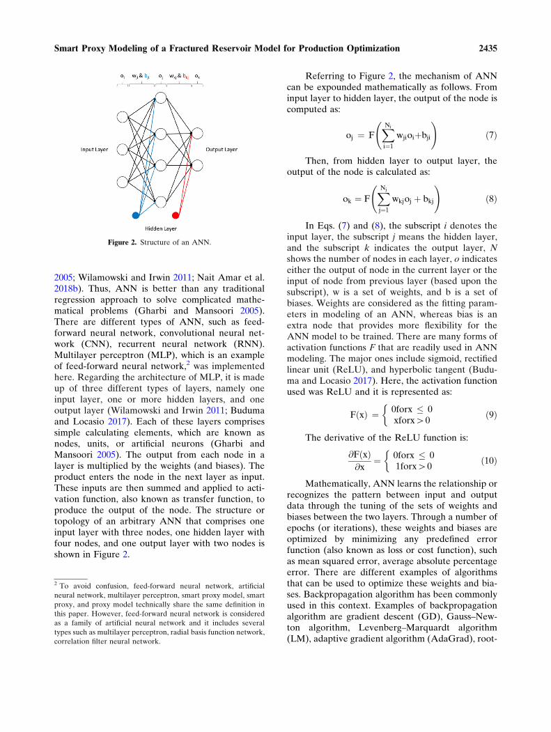
2005; Wilamowski and Irwin 2011; Nait Amar et al.2018b). Thus, ANN is better than any traditionalregression approach to solve complicated mathe-matical problems (Gharbi and Mansoori 2005).There are different types of ANN, such as feed-forward neural network, convolutional neural net-work (CNN), recurrent neural network (RNN).Multilayer perceptron (MLP), which is an exampleof feed-forward neural network,2 was implementedhere. Regarding the architecture of MLP, it is madeup of three different types of layers, namely oneinput layer, one or more hidden layers, and oneoutput layer (Wilamowski and Irwin 2011; Budumaand Locasio 2017). Each of these layers comprisessimple calculating elements, which are known asnodes, units, or artificial neurons (Gharbi andMansoori 2005). The output from each node in alayer is multiplied by the weights (and biases). Theproduct enters the node in the next layer as input.These inputs are then summed and applied to acti-vation function, also known as transfer function, toproduce the output of the node. The structure ortopology of an arbitrary ANN that comprises oneinput layer with three nodes, one hidden layer withfour nodes, and one output layer with two nodes isshown in Figure 2.

Referring to Figure 2, the mechanism of ANNcan be expounded mathematically as follows. Frominput layer to hidden layer, the output of the node iscomputed as:

oj ¼ FXNi

i¼1

wjioiþbji

!ð7Þ

Then, from hidden layer to output layer, theoutput of the node is calculated as:

ok ¼ FXNj

j¼1

wkjoj þ bkj

!ð8Þ

In Eqs. (7) and (8), the subscript i denotes theinput layer, the subscript j means the hidden layer,and the subscript k indicates the output layer, Nshows the number of nodes in each layer, o indicateseither the output of node in the current layer or theinput of node from previous layer (based upon thesubscript), w is a set of weights, and b is a set ofbiases. Weights are considered as the fitting param-eters in modeling of an ANN, whereas bias is anextra node that provides more flexibility for theANN model to be trained. There are many forms ofactivation functions F that are readily used in ANNmodeling. The major ones include sigmoid, rectifiedlinear unit (ReLU), and hyperbolic tangent (Budu-ma and Locasio 2017). Here, the activation functionused was ReLU and it is represented as:

F xð Þ ¼ 0forx � 0xforx[0

�ð9Þ

The derivative of the ReLU function is:

@F xð Þ@x

¼ 0forx � 01forx[0

�ð10Þ

Mathematically, ANN learns the relationship orrecognizes the pattern between input and outputdata through the tuning of the sets of weights andbiases between the two layers. Through a number ofepochs (or iterations), these weights and biases areoptimized by minimizing any predefined errorfunction (also known as loss or cost function), suchas mean squared error, average absolute percentageerror. There are different examples of algorithmsthat can be used to optimize these weights and bia-ses. Backpropagation algorithm has been commonlyused in this context. Examples of backpropagationalgorithm are gradient descent (GD), Gauss–New-ton algorithm, Levenberg–Marquardt algorithm(LM), adaptive gradient algorithm (AdaGrad), root-

Figure 2. Structure of an ANN.

2 To avoid confusion, feed-forward neural network, artificial

neural network, multilayer perceptron, smart proxy model, smart

proxy, and proxy model technically share the same definition in

this paper. However, feed-forward neural network is considered

as a family of artificial neural network and it includes several

types such as multilayer perceptron, radial basis function network,

correlation filter neural network.


mean-square propagation (RMSProp), Adam, andso forth. Additionally, other metaheuristic algo-rithms, like PSO, DE, genetic algorithm (GA), andso forth, have also been proven useful for neuralnetwork training (Nait Amar et al. 2018a, b). AsBianchi et al. (2009) have counseled, metaheuristicalgorithm is a high-level mathematical algorithmthat is generally natural inspired and used to solvemore sophisticated optimization problems. In thisstudy, both backpropagation algorithm and meta-heuristic approach have been employed to enablethe ANN to ‘‘learn.’’ The selected backpropagationalgorithm was GD, whereas PSO was the chosenmetaheuristic training algorithm.

Backpropagation Algorithm

For the workflow of the GD algorithm, both theinputs and outputs are fed to the ANN as thetraining phase starts. When the inputs enter theANN and proceed through the layers, they aregradually processed to yield the predicted output.Thereafter, the predicted output is compared withthe desired output. Errors are then propagated backthrough the ANN. During this backpropagation, theweights and biases are adjusted to minimize the er-rors. Such process is repeated iteratively until eitherthe errors become less than the predefined toleranceor the number of iterations is reached. The GD is analgorithm that applies the first-order derivative forcomputation. In this context, the first-order deriva-tive of the error function is implemented to deter-mine the minimum in the error space. Thecalculation of gradient at iteration t can be ex-pressed mathematically as:

gt ¼@E x;wtð Þ

@wt¼ @E

@w1;t

@E

@w2;t

@E

@w3;t. . .

@E

@wN;t

� �Tð11Þ

where E indicates the error function, x the inputvector, and w the weight (and bias) vector. There-after, the weights are updated by using the followingequations. The same idea applies to the updating ofthe biases.

wtþ1 ¼ wt þ Dwt ð12Þ

wtþ1 ¼ wt � c� gtð Þ ð13ÞIn Eqs. (12) and (13), the weights (and biases)

at iteration t + 1 are updated using the weights (andbiases) at iteration t, the gradient at t, and c, which is

the learning rate or step size. Therefore, the gradientis always computed at every iteration step to adjustthe weights (and biases). Pertaining to the compu-tation of gradient of error function, it is highlydependent on the forms of error function and acti-vation function that were used. Here, the errorfunction used was the mean squared error, whereasthe activation function used was ReLU.

The mathematical formulation of the applica-tion of GD as learning algorithm is as follows. Forthe following derivation, the meaning of the sub-scripts used here is the same as explained above. Theterm tmeans the target value or the actual output, P,denotes the total number of training sets provided;thus:

E x; w; bð Þ ¼ 1

P

XPk¼ 1

tk � okð Þ2 ð14Þ

Having defined the error function, the back-propagation algorithm starts by computing theweight update between the hidden and output lay-ers. To perform this computation, the gradient of theerror function with respect to the weights betweenthe hidden and output layers is determined. There-after, the similar procedure is conducted to calculatethe weight update between the hidden and inputlayer. This algorithm carries on iteratively until thevalue of error function (obtained by using the up-dated weights and biases) is less than a predefinedtolerance or the initialized number of epochs isreached. For a more substantial understanding ofthe mathematical formulation of the backpropaga-tion algorithm, peruse Wilamowski and Irwin (2011)and the relevant literatures. Here, the Keras mod-ule, which was developed by Chollet (2019), hadbeen implemented with the help of the programminglanguage Python 3.8.1 and TensorFlow 2.1.0 to usethe GD algorithm to optimize the weights and bia-ses. However, it is essential to note that in Kerasmodule, instead of using GD algorithm, thestochastic gradient descent (SGD) algorithm is ap-plied. The fundamentals of these two algorithms arethe same. The main difference is that, in SGD, thegradient is only computed once at each iteration step(by randomly selecting a sample from the trainingset) and is used further (Buduma and Locasio 2017).By inducing this stochastic behavior, the computa-tional cost is reduced drastically. Apart from SGD,Adam was another backpropagation algorithm usedhere; it is a more advanced and robust variant ofSGD developed by Kingma and Ba (2015). Mathe-


matically, it approximates the first and second mo-ments of gradients to adaptively calculate thelearning rates for different parameters (Kingma andBa 2015). Refer to Kingma and Ba (2015) for thedetails of Adam. Here, Adam was also implementedusing Python 3.8.1 and TensorFlow 2.1.0.

PSO

PSO was introduced by Kennedy et al. (1995)based upon the simulation of the social behavior of aflock of flying birds. As explained in several litera-tures (Kennedy et al. 1995; Shi and Eberhart 1999;Nait Amar et al. 2018a), mathematically, this algo-rithm operates by having a population of particles,which is also known as a swarm of particles. Each ofthese particles corresponds to a potential position ora solution in a search space. Then, the position ofeach particle is updated iteratively according to itsposition and velocity at previous timestep. Themovements of the particles in the search space arecontrolled by their own best-known position (thelocal best position) and their best-known position inthe entire swarm (the global best position). As thisprocess occurs iteratively, the particles in the swarmwill eventually converge to an optimal point, whichis deemed as the best solution in the search space.The position and velocity for the jth particle in a N-dimensional space at iteration t can be expressed,respectively, as:

xj;t ¼ xj1;t; xj2;t; xj3;t; . . . ; xjN;t

� �ð15Þ

vj;t ¼ vj1;t; vj2;t; vj3;t; . . . ; vjN;t

� �ð16Þ

Then, the velocity of each particle at next iter-ation t + 1 is updated as (Shi and Eberhart 1999):

vjN;tþ1 ¼ vjN;t þ c1r1 pbestjN;t � xjN;t

þ c2r2 gbestN;t � xjN;t

ð17Þ

In Eqs. (15), (16), and (17), vjN,t and xjN,t rep-resent the velocity of the jth particle at iteration tand its corresponding position in N-dimensionquantity, respectively; pbestjN,t corresponds to theN-dimension quantity of the individual j at the bestposition or the local best position at iteration t;gbestN,t is the N-dimension quantity of the swarm atthe best position or the global best position at iter-ation t; c1 denotes the cognitive learning factor (alsoknown as cognitive weight), whereas c2 means the

social learning factor (also known as social weight);r1 and r2 are random numbers extracted between 0and 1. Upon updating the velocity, each particlemoves to a new potential solution as:

xjN;tþ1 ¼ xjN;t þ vjN;tþ1 ð18Þ

A new parameter, inertial weight x introducedby Shi and Eberhart (1998), was included in Eq. (17)to improve the convergence condition. This alsogradually decreases the velocity of the particles tohave the swarm of particles under control (NaitAmar et al. 2018a). In other words, it plays a part inbalancing the global search also known as explo-ration, and the local search also termed asexploitation (Shi and Eberhart 1998; Zhang et al.2015):

vjN;tþ1 ¼ xvjN;t þ c1r1 pbestjN;t � xjN;t

þ c2r2 gbestN;t � xjN;t

: ð20Þ

In the context of the minimization problem, anobjective function f to be minimized is defined.Then, to determine the local best solution at itera-tion t + 1, the following formula is given (Nait Amaret al. 2018a):

pbestjN;tþ1 ¼pbestjN;t; iff ðpbestjN;tÞ ¼ fðxjN;tþ1Þ

xjN;tþ1; otherwise

�

ð21ÞThen, to find the global best solution at itera-

tion t + 1, the following mathematical formulation ispresented:

gbestjN;tþ1 ¼ min f pbestjN;tþ1

h ið22Þ

In this study, the objective function was theerror function in the ANN modeling. To apply PSOas the training algorithm of ANN, this can be simplydone by treating the weights and biases as the par-ticles in the algorithm. Hence, the total number ofparticles in a swarm is the total number of weightsand biases. Then, the optimization can be performedusing the abovementioned formulations. Here, thepackage of PySwarms version 1.1.0, which was builtby Miranda (2019), was implemented by using theprogramming language Python 3.8.1 to perform theoptimization. In comparison with the SGD algo-rithm, one of the advantages of PSO is that it is aderivative-free algorithm. This implies that it is morerobust as it can be utilized to optimize a mathe-matical function that is not easily differentiable.


NUMERICAL SIMULATION MODEL

A three-dimensional, two-phase (black oil andwater) reservoir simulation model was built to rep-resent the ‘‘true’’ reservoir model. The ‘‘true’’reservoir is in fact inspired by the dual-porositymodel discussed in Firoozabadi and Thomas (1990),which is a two-dimensional and three-phase model(black oil, water, and gas—including free and dis-solved gas). However, most of the reservoir param-eters and relevant fluid properties were changed todevelop the ‘‘true’’ model. This ‘‘true’’ reservoirmodel supplied the necessary data for the develop-ment of the respective SPM. This reservoir was aDPDP model made up of three layers with uniformthickness.3 The top of this reservoir was set at thedepth of 305 m. About the geometry of this model,each grid block had a length of 25 m, a width of25 m, and a height of 15.2 m. Thus, the dimension ofthe reservoir model was 1525 m 9 1525 m 9 45.7m, which corresponds to the number of blocks being61 9 61 9 3. Regarding the well configuration, itwas the five-spot pattern in which four injectorswere, respectively, set to penetrate near the cornersof this reservoir model and a producer was placed in

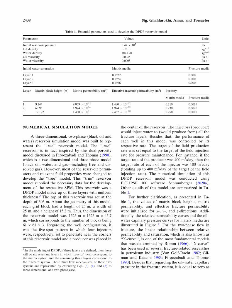
the center of the reservoir. The injectors (producer)would inject water to (would produce from) all thefracture layers. Besides that, the performance ofeach well in this model was controlled by itsrespective rate. The target of the field productionrate was set equal to the target of the field injectionrate for pressure maintenance. For instance, if thetarget rate of the producer was 400 m3/day, then thetarget rate of each of the injector was 100 m3/day(totaling up to 400 m3/day of the target of the fieldinjection rate). The numerical simulation of thisDPDP reservoir model was conducted usingECLIPSE 100 software Schlumberger (2020a).Other details of this model are summarized in Ta-ble 1.

For further clarification, as presented in Ta-ble 1, the values of matrix block heights, matrixpermeability, and effective fracture permeabilitywere initialized for x-, y-, and z-directions. Addi-tionally, the relative permeability curves and the oil–water capillary pressure curves for matrix media areillustrated in Figure 3. For the two-phase flow infracture, the linear relationship between relativepermeability and saturation, which is also known as‘‘X-curve’’, is one of the most fundamental modelsthat was determined by Romm (1966). ‘‘X-curve’’has been used in several fracture-related researchesin petroleum industry (Van Golf-Racht 1982; Gil-man and Kazemi 1983; Firoozabadi and Thomas1990). Besides that, regarding the oil–water capillarypressure in the fracture system, it is equal to zero as

Table 1. Essential parameters used to develop the DPDP reservoir model

Parameters Values Units

Initial reservoir pressure 3.47 9 107 Pa

Oil density 819.18 kg/m3

Water density 1041.20 kg/m3

Oil viscosity 0.0035 Pa s

Water viscosity 0.0005 Pa s

Initial water saturation Matrix media Fracture media

Layer 1 0.1922 0.000

Layer 2 0.1924 0.000

Layer 3 0.1926 0.000

Layer Matrix block height (m) Matrix permeability (m2) Effective fracture permeability (m2) Porosity

Matrix media Fracture media

1 9.144 9.869 9 10-15 1.480 9 10�12 0.210 0.0015

2 6.096 1.974 9 10-14 1.974 9 10�12 0.230 0.0020

3 12.192 1.480 9 10-14 2.467 9 10�12 0.250 0.0018

3 In the modeling of DPDP, if three layers are defined, then there

will be six resultant layers in which three of them correspond to

the matrix system and the remaining three layers correspond to

the fracture system. These fluid flow mechanisms of these two

systems are represented by extending Eqs. (3), (4), and (5) to

three-dimensional and two-phase case.


shown in the model discussed by Firoozabadi andThomas (1990). In short, we selected these models ofrelative permeability curve and oil–water capillarypressure in both matrix and fracture systems forillustrative purpose. By using the software ResIn-sight developed by Ceetron Solution AS (2020), thisreservoir model depicting oil saturation at the waterinjection rate of 636 m3/day (after the injectionperiod of 5 years) is displayed correspondingly inFigure 4 for the matrix system and in Figure 5 forthe fracture system.

Based on Figures 4 and 5, much more oil hadbeen swept toward the producers in Layer 3 for bothmatrix and fracture media. Because the injectors

were (the producer was) perforated in all the frac-ture layers, this denoted that the injected water flo-wed and swept the oil in (the oil was only producedfrom) the fracture systems. Given the homogeneityof every layer of the model and the high effectivepermeabilities in z-direction for all the fracturelayers, the cross-flow of fluids between the fracturelayers was prominent to contribute to the highsweeping of oil in Layer 3 of the fracture media. Thisscenario also occurred to the matrix media becauseit needed to supply the oil to the fracture systemwhere most of the oil has been swept and produced.In this context, we reiterate that the DPDP reservoirmodeling was not the main goal of this work. In fact,we intended to design a valid DPDP model to

(a) (b)

0.00E+00

1.00E-16

2.00E-16

3.00E-16

4.00E-16

5.00E-16

6.00E-16

7.00E-16

8.00E-16

0.000 0.200 0.400 0.600 0.800

Rel

ativ

e Pe

rmea

bilit

y (m

2 )

Water Saturation

Water Oil

0.00E+00

1.00E+06

2.00E+06

3.00E+06

4.00E+06

5.00E+06

6.00E+06

0.000 0.200 0.400 0.600 0.800

Cap

illar

y Pr

essu

re C

urve

(Pa)

Water Saturation

Figure 3. (a) Relative permeability curve. (b) Oil–water capillary pressure curve for the matrix media.

Figure 4. Overview of the matrix system of the reservoir

model: (a) Layer 1; (b) Layer 2; (c) Layer 3.

Figure 5. Overview of the fracture system of the reservoir

model: (a) Layer 1; (b) Layer 2; (c) Layer 3.


demonstrate that our developed proxy model wasfunctioning accurately.

PRODUCTION OPTIMIZATION

Smart proxy is widely developed in the petro-leum industry because of its inexpensive computa-tional effort. However, SPM is an objective-orientedtask, which implies that modelers need to first knowwhat the smart proxy is used for prior to developing

it. After identifying the purposes or functions of themodel, modelers would have a well-establishedunderstanding pertaining to the preparation of thespatio-temporal database (input and output data)used for neural network training. Regarding this, weused an illustrative example of production opti-mization as the objective of developing the smartproxy. For this illustrative example, we assumed theproduction lifetime of the reservoir model discussed

Table 2. Values of the economic parameters used in this example

of production optimization

Parameters Values Units

Oil price, Po 377.40 USD/m3

Cost of produced water, Pw 44.02

Cost of injected water, Pinj 44.02

Monthly discounted rate 0.833 %

Table 3. Simulation scenarios executed for SPM

Scenario Index Injection rate (m3/day)

1 636

2 676

3 715

4 755

5 795

Figure 6. General workflow of SPM.


to be 30 years and the objective function to be thenet present value (NPV). In this case, we needed todecide the target of the field injection rate that canmaximize the NPV throughout the production life-time. The NPV for this optimization example can beformulated as:

NPV ¼XN

k¼ 0

PoQo;k � PwQw;k � PinjQinj;k

ð1 þ rÞkð23Þ

where the subscripts o, w, and inj denote oil, water(produced), and injected water, respectively; P is theprice (or cost) per standard barrel (the correspond-ing unit is USD/m3), Q is total amount for a certaintimestep (the respective unit is m3), r is the discountrate, and k is the timestep. To calculate Q, the fol-lowing equation was used:

Qi� o;w;injf g;k ¼ qi� o;w;injf g;k � Dtk ð24Þ

where q is the flow rate reported (either by thenumerical simulation or the developed SPM) onmonthly basis (the unit is m3/day) and Dtk is thenumber of months for timestep k. Here, the smartproxy for the prediction of injection rates was notdeveloped as the injection rates remained constantthroughout the production period of the reservoirmodel. Hence, for practical purpose, only two SPMswere developed, which, respectively, predicted theoil production rates and the water production rates(both on monthly basis). With respect to this, it ispossible to develop a SPM that predicts simultane-ously two outputs, namely both oil and water rates.Nevertheless, the tuning of the weights and biasescan be more challenging. Thus, for better and morefundamental demonstration of SPM, we decided not

to go with this option in this work. Upon formulatingthe objective function used in this example of pro-duction optimization, the setting of the economicparameters4 used is presented in Table 2.

SMART PROXY MODELING

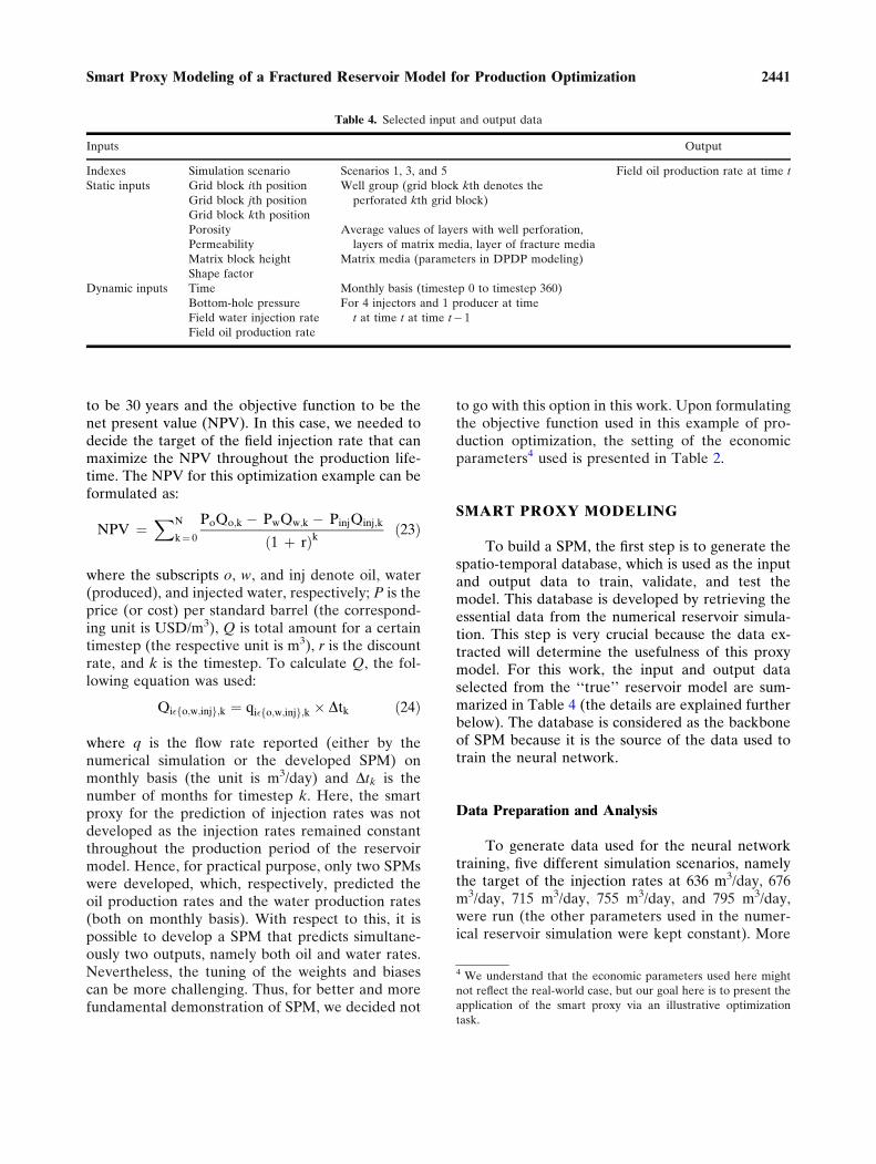
To build a SPM, the first step is to generate thespatio-temporal database, which is used as the inputand output data to train, validate, and test themodel. This database is developed by retrieving theessential data from the numerical reservoir simula-tion. This step is very crucial because the data ex-tracted will determine the usefulness of this proxymodel. For this work, the input and output dataselected from the ‘‘true’’ reservoir model are sum-marized in Table 4 (the details are explained furtherbelow). The database is considered as the backboneof SPM because it is the source of the data used totrain the neural network.

Data Preparation and Analysis

To generate data used for the neural networktraining, five different simulation scenarios, namelythe target of the injection rates at 636 m3/day, 676m3/day, 715 m3/day, 755 m3/day, and 795 m3/day,were run (the other parameters used in the numer-ical reservoir simulation were kept constant). More

Table 4. Selected input and output data

Inputs Output

Indexes Simulation scenario Scenarios 1, 3, and 5 Field oil production rate at time t

Static inputs Grid block ith position Well group (grid block kth denotes the

perforated kth grid block)Grid block jth position

Grid block kth position

Porosity Average values of layers with well perforation,

layers of matrix media, layer of fracture mediaPermeability

Matrix block height Matrix media (parameters in DPDP modeling)

Shape factor

Dynamic inputs Time Monthly basis (timestep 0 to timestep 360)

Bottom-hole pressure For 4 injectors and 1 producer at time

t at time t at time t� 1Field water injection rate

Field oil production rate

4 We understand that the economic parameters used here might

not reflect the real-world case, but our goal here is to present the

application of the smart proxy via an illustrative optimization

task.


precisely, only three of them were used for thedevelopment of smart proxy, whereas the remainingtwo were used as the blind cases, which are discussedfurther below. Table 3 summarizes the five simula-tion scenarios, of which scenarios 1, 3, and 5 wereused for SPM.

Upon running the simulations, the spatio-tem-poral database was readily generated. This databasewas developed by extracting the static and dynamicdata from the numerical simulation. In this context,static data indicate that the data do not change withtime (e.g., porosity, permeability), whereas dynamicdata denote otherwise (e.g., instance, water injectionrate, oil production rate). One of the main chal-lenges of SPM is the humongous size of the spatio-temporal database. This occurs when the geologicalproperties (static properties) of the simulatedreservoir model are very heterogeneous (each of thegrid blocks in the reservoir model has differentvalues of porosity and permeability). The high geo-logical heterogeneity will cause the SPM to beimpractical if all these static data are used. To alle-viate this problem, several literatures (Mohagheghet al. 2012a, b, c, 2015; He et al. 2016; Alenezi andMohaghegh 2016, 2017) recommend the applicationof tier system to delineate the reservoir model. Inthis aspect, the Voronoi graph theory was imple-mented to re-upscale these static properties throughthe lumping of the reservoir layers. By doing so, thesize of the static inputs used in defining the structureof the spatio-temporal database can be decreased.However, here, despite having a total of 22,326 gridblocks in the reservoir model, it was not consideredto be very complex because the porosity and per-meability were homogenous per layer. Hence, thereservoir model can be simply delineated by cate-gorizing it into the matrix media and fracture media.

After resolving the issue of reservoir complex-ity, the selection of input and output data needs tobe considered. For a real-life reservoir model, thespatio-temporal database can still be gigantic to beentirely used as the input and output for SPM. Tomitigate this challenge, the above-mentioned litera-tures propose to use the key performance indicator(KPI) coupled with fuzzy logic to help rank the de-gree of influence of different properties in theselection of input and output, and it is conductedmostly by using commercial software. In this study,for the purpose of illustration, the input and outputdata for SPM were determined based upon ourknowledge of reservoir engineering. Thereafter, theinput and output data yielded the final database

applied for training, validating, and testing theneural network as summarized in Table 4, whichshows 54 static inputs and 8 dynamic inputs.

On the one hand, regarding static properties,the scenario index, which helps the neural networkto identify which instance of the injection rates isused, was one of them. Besides this, the well loca-tions make up 25 out of 54 static inputs becausethere were 5 wells in total and each of the locationswas represented as ith, jth, and kth positions of thegrid blocks (with all the fracture layers perforated).This corresponded to one group of the static inputs(Table 4). For both porosity and permeability, eachof them comprised 11 static inputs, and 5 of themcorresponded to the inputs of the average values ofgrid block where the wells were perforated and theremaining 6 corresponded to the inputs for the 3layers in both matrix and fracture systems. There-after, the heights of the matrix blocks and the shapefactors, respectively, contributed to 3 static inputs.

On the other hand, the bottom-hole pressuresof all 5 wells contributed to 5 of the 8 dynamic in-puts. Besides that, the timestep also acted as one ofthe dynamic inputs. The water injection rate at timet (on monthly basis) was also a dynamic input. Theremaining dynamic input was the oil production rateat time t� 1 (on monthly basis), whereas the oilproduction rate at time t (on monthly basis) wasused as the output data instead of being treated asinput data in this neural network training. For thedevelopment of smart proxy for the prediction ofwater production rates, the input and output datawere essentially the same. However, only the oilproduction rates at time t� 1 and t needed to bereplaced with the water production rates at time t1 and t. Besides that, each of the simulation sce-narios was run for 30 years. Since the oil productionrates were reported on monthly basis, this corre-sponded to 360 months (30 years � 12 months/year). By starting from timestep = 0, there were atotal of 361 timesteps for each scenario. This re-sulted in a total number of 68,229 records (3 sce-narios � 361 timesteps/scenario � 63records/timestep) in the database, which was to befed into the neural network for training.

Neural Network Training

Training the neural network is the most essen-tial part of SPM. Prior to feeding the input and


output data into the ANN for training, the databaseis normalized between 0 and 1, thus:

xnormalized ¼ xi � xmin

xmax � xminð25Þ

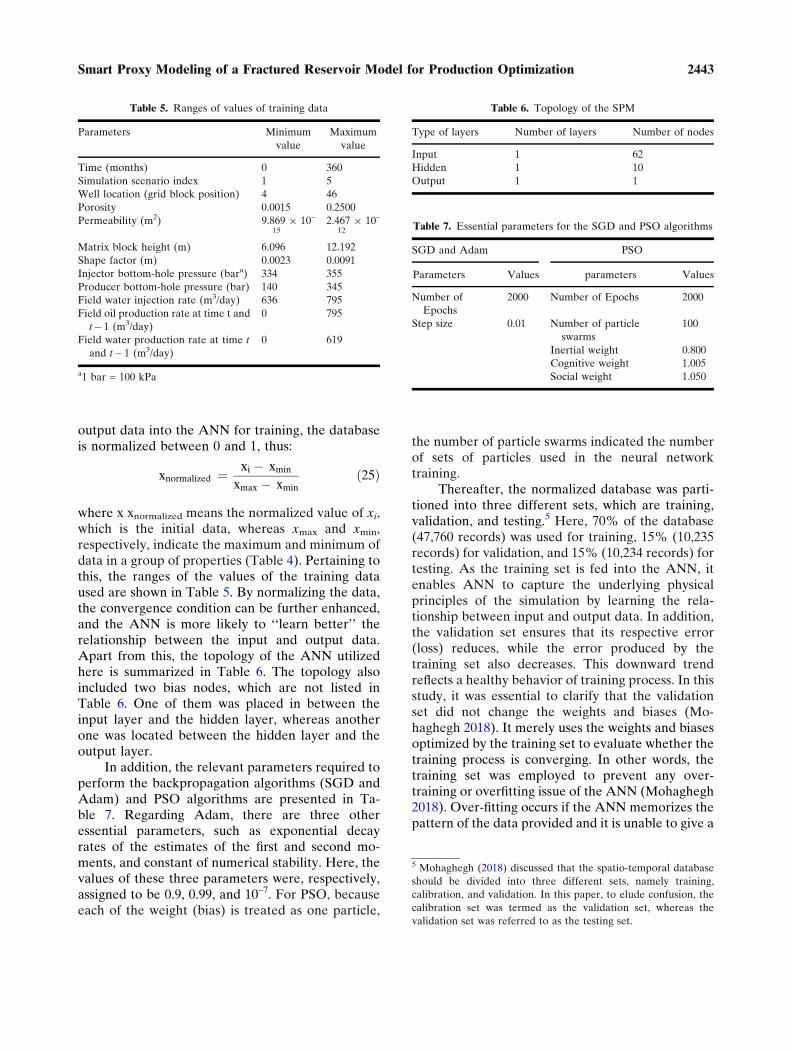
where x xnormalized means the normalized value of xi,which is the initial data, whereas xmax and xmin,respectively, indicate the maximum and minimum ofdata in a group of properties (Table 4). Pertaining tothis, the ranges of the values of the training dataused are shown in Table 5. By normalizing the data,the convergence condition can be further enhanced,and the ANN is more likely to ‘‘learn better’’ therelationship between the input and output data.Apart from this, the topology of the ANN utilizedhere is summarized in Table 6. The topology alsoincluded two bias nodes, which are not listed inTable 6. One of them was placed in between theinput layer and the hidden layer, whereas anotherone was located between the hidden layer and theoutput layer.

In addition, the relevant parameters required toperform the backpropagation algorithms (SGD andAdam) and PSO algorithms are presented in Ta-ble 7. Regarding Adam, there are three otheressential parameters, such as exponential decayrates of the estimates of the first and second mo-ments, and constant of numerical stability. Here, thevalues of these three parameters were, respectively,assigned to be 0.9, 0.99, and 10–7. For PSO, becauseeach of the weight (bias) is treated as one particle,

the number of particle swarms indicated the numberof sets of particles used in the neural networktraining.

Thereafter, the normalized database was parti-tioned into three different sets, which are training,validation, and testing.5 Here, 70% of the database(47,760 records) was used for training, 15% (10,235records) for validation, and 15% (10,234 records) fortesting. As the training set is fed into the ANN, itenables ANN to capture the underlying physicalprinciples of the simulation by learning the rela-tionship between input and output data. In addition,the validation set ensures that its respective error(loss) reduces, while the error produced by thetraining set also decreases. This downward trendreflects a healthy behavior of training process. In thisstudy, it was essential to clarify that the validationset did not change the weights and biases (Mo-haghegh 2018). It merely uses the weights and biasesoptimized by the training set to evaluate whether thetraining process is converging. In other words, thetraining set was employed to prevent any over-training or overfitting issue of the ANN (Mohaghegh2018). Over-fitting occurs if the ANN memorizes thepattern of the data provided and it is unable to give a

Table 5. Ranges of values of training data

Parameters Minimum

value

Maximum

value

Time (months) 0 360

Simulation scenario index 1 5

Well location (grid block position) 4 46

Porosity 0.0015 0.2500

Permeability (m2) 9.869 9 10–

152.467 9 10–

12

Matrix block height (m) 6.096 12.192

Shape factor (m) 0.0023 0.0091

Injector bottom-hole pressure (bara) 334 355

Producer bottom-hole pressure (bar) 140 345

Field water injection rate (m3/day) 636 795

Field oil production rate at time t and

t� 1 (m3/day)

0 795

Field water production rate at time t

and t� 1 (m3/day)

0 619

a1 bar = 100 kPa

Table 6. Topology of the SPM

Type of layers Number of layers Number of nodes

Input 1 62

Hidden 1 10

Output 1 1

Table 7. Essential parameters for the SGD and PSO algorithms

SGD and Adam PSO

Parameters Values parameters Values

Number of

Epochs

2000 Number of Epochs 2000

Step size 0.01 Number of particle

swarms

100

Inertial weight 0.800

Cognitive weight 1.005

Social weight 1.050

5 Mohaghegh (2018) discussed that the spatio-temporal database

should be divided into three different sets, namely training,

calibration, and validation. In this paper, to elude confusion, the

calibration set was termed as the validation set, whereas the

validation set was referred to as the testing set.


good prediction when other data are supplied. Thetesting set assists in checking the predictability of thetrained neural network.

After the trained ANN was evaluated by thetesting set, it should be provided with a new set ofdata (that were not from the database) to perform ablind case run. This step is crucial to further confirmthe robustness of the developed SPM. Once the re-

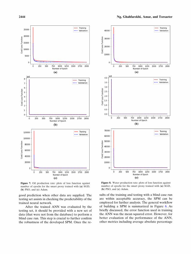
sults of the training and testing with a blind case runare within acceptable accuracy, the SPM can beemployed for further analysis. The general workflowof building a SPM is summarized in Figure 6. Asbriefly discussed, the error function used in trainingthe ANN was the mean squared error. However, forbetter evaluation of the performance of the ANN,other metrics including average absolute percentage

Figure 7. Oil production rate: plots of loss function against

number of epochs for the smart proxy trained with (a) SGD,

(b) PSO, and (c) Adam.

Figure 8. Water production rate: plots of loss function against

number of epochs for the smart proxy trained with (a) SGD,

(b) PSO, and (c) Adam.


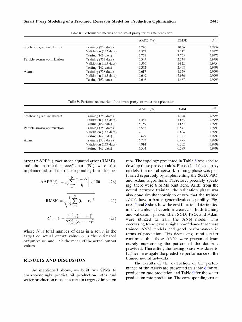
error (AAPE%), root-mean-squared error (RMSE),and the correlation coefficient (R2) were alsoimplemented, and their corresponding formulas are:

AAPEð%Þ ¼ 1

N

XNi¼ 1

ti � oiti

�� 100 ð26Þ

RMSE ¼

ffiffiffiffiffiffiffiffiffiffiffiffiffiffiffiffiffiffiffiffiffiffiffiffiffiffiffiffiffiffiffiffi1

N

XNi¼1

ti � oið Þ2vuut ð27Þ

R2 ¼ 1 �PN

i¼1 ti � oið Þ2PNi¼1 oi � �tð Þ2

ð28Þ

where N is total number of data in a set, ti is thetarget or actual output value, oi is the estimatedoutput value, and �t is the mean of the actual outputvalues.

RESULTS AND DISCUSSION

As mentioned above, we built two SPMs tocorrespondingly predict oil production rates andwater production rates at a certain target of injection

rate. The topology presented in Table 6 was used todevelop these proxy models. For each of these proxymodels, the neural network training phase was per-formed separately by implementing the SGD, PSO,and Adam algorithms. Therefore, precisely speak-ing, there were 6 SPMs built here. Aside from theneural network training, the validation phase wasalso done simultaneously to ensure that the trainedANNs have a better generalization capability. Fig-ures 7 and 8 show how the cost function deterioratedas the number of epochs increased in both trainingand validation phases when SGD, PSO, and Adamwere utilized to train the ANN model. Thisdecreasing trend gave a higher confidence that thesetrained ANN models had good performances interms of prediction. This decreasing trend furtherconfirmed that these ANNs were prevented frommerely memorizing the pattern of the databaseprovided. Thereafter, the testing phase was done tofurther investigate the predictive performance of thetrained neural networks.

The results of the evaluation of the perfor-mance of the ANNs are presented in Table 8 for oilproduction rate prediction and Table 9 for the waterproduction rate prediction. The corresponding cross-

Table 8. Performance metrics of the smart proxy for oil rate prediction

AAPE (%) RMSE R2

Stochastic gradient descent Training (758 data) 1.770 10.66 0.9954

Validation (163 data) 1.567 7.512 0.9977

Testing (162 data) 1.768 7.769 0.9971

Particle swarm optimization Training (758 data) 0.349 2.378 0.9998

Validation (163 data) 0.536 14.22 0.9934

Testing (162 data) 0.352 2.408 0.9998

Adam Training (758 data) 0.617 1.829 0.9999

Validation (163 data) 0.649 2.036 0.9998

Testing (162 data) 0.646 1.487 0.9999

Table 9. Performance metrics of the smart proxy for water rate prediction

AAPE (%) RMSE R2

Stochastic gradient descent Training (758 data) – 1.728 0.9998

Validation (163 data) 6.461 1.685 0.9998

Testing (162 data) 8.159 1.652 0.9999

Particle swarm optimization Training (758 data) 6.565 0.547 0.9999

Validation (163 data) – 0.864 0.9999

Testing (162 data) 7.629 0.761 0.9999

Adam Training (758 data) 6.753 0.475 0.9999

Validation (163 data) 4.914 0.262 0.9999

Testing (162 data) 6.504 0.389 0.9999


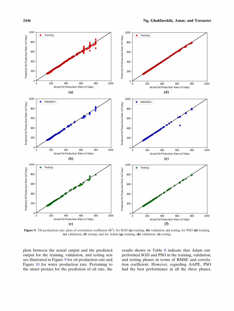
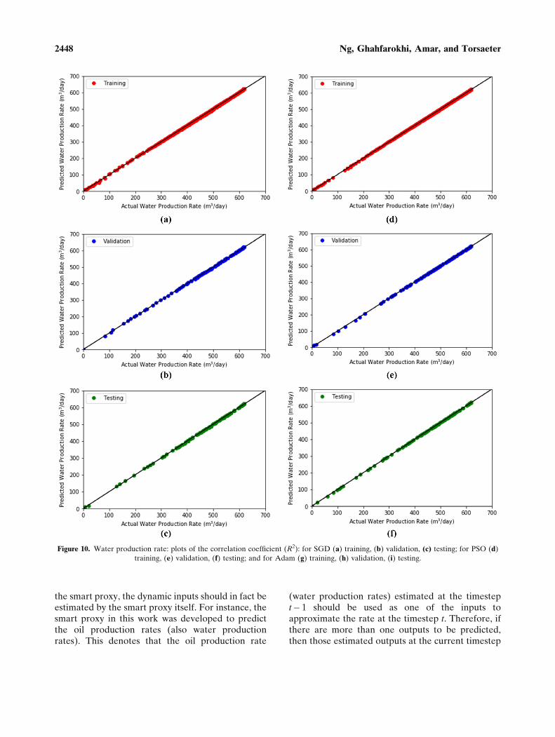
plots between the actual output and the predictedoutput for the training, validation, and testing setsare illustrated in Figure 9 for oil production rate andFigure 10 for water production rate. Pertaining tothe smart proxies for the prediction of oil rate, the

results shown in Table 8 indicate that Adam out-performed SGD and PSO in the training, validation,and testing phases in terms of RMSE and correla-tion coefficient. However, regarding AAPE, PSOhad the best performance in all the three phases.

Figure 9. Oil production rate: plots of correlation coefficient (R2): for SGD (a) training, (b) validation, (c) testing; for PSO (d) training,(e) validation, (f) testing; and for Adam (g) training, (h) validation, (i) testing.


Additionally, better performance of Adam is alsopresented in Figure 9. As it can be observed, muchmore data samples lie on the 45-degree line as theAdam was used to develop the smart proxies com-pared to the cases where the SGD and PSO wereutilized. Hence, Adam generally had the best per-formance, whereas PSO performed better than

SGD. Nonetheless, in the validation phase, SGDperformed better than the PSO in terms of theminimization of RMSE and the maximization of thecorrelation coefficient. This can be due to the exis-tence of an over-estimated data point (an outlier) inthe validation phase of PSO (as shown in Figure 9e).Because the healthy training process is illustrated inFigure 7, it was deduced that any of these trainedmodels was sufficiently good to be applied to predictthe oil production rate. This is further justified bythe results of the performance metrics in Table 8,which indicate that the correlation coefficients yiel-ded by all the datasets exceeded 0.99 and bothAAPEs and RMSEs exhibited in all the phases wereconsiderably low.

For the prediction of water production rate (asillustrated in Figure 10), it is difficult to infer whe-ther the backpropagation algorithm or the PSOyielded a better performance in the training, vali-dation, and testing phases. However, according to,Adam generally had the best results as comparedwith SGD and PSO, whereas PSO performed betterthan SGD. In addition, the results of AAPE werenot provided for the training phase of SGD and thevalidation phase of PSO because, in these phases,there were a few over-estimated data points (out-liers) that caused the AAPE to be very large (morethan 1000%). This is because when these data pointswere selected at the early stage of water break-through, the actual water production rate was veryminiscule. Based on Eq. (26), if the numerator is inthe order of magnitude of 1 or 10, then the AAPEwill increase drastically. Thus, for practical reasons,the results were not shown here. Despite this, thisscenario provided an insight that we needed to lookat different performance metrics during SPM todetermine whether the built proxy models func-tioned satisfactorily. Besides, these outliers did notaffect the overall predictive capability of the smartproxy built here as the model was still able to cap-ture the general data pattern during the develop-ment stage as presented in Figure 10.

After developing the SPMs, two blind caseswere run by using the target of the injection rates at676 m3/day and 755 m3/day to provide moreinsightful ideas regarding the usefulness of thetrained smart proxies. In other words, the spatio-temporal databases when the target of the injectionrates was, respectively, at 676 m3/day and 755m3/day created to be fed into the smart proxies toobserve how well they can make predictions. It isessential to know that, in order to practically apply

Figure 9. continued.


the smart proxy, the dynamic inputs should in fact beestimated by the smart proxy itself. For instance, thesmart proxy in this work was developed to predictthe oil production rates (also water productionrates). This denotes that the oil production rate

(water production rates) estimated at the timestept� 1 should be used as one of the inputs toapproximate the rate at the timestep t. Therefore, ifthere are more than one outputs to be predicted,then those estimated outputs at the current timestep

Figure 10. Water production rate: plots of the correlation coefficient (R2): for SGD (a) training, (b) validation, (c) testing; for PSO (d)

training, (e) validation, (f) testing; and for Adam (g) training, (h) validation, (i) testing.


should be cascaded simultaneously to be the inputsat the next timestep. Alternatively, different smartproxy can be designed specifically to provide a pre-

diction of any of the outputs, which is used as theinput for another smart proxy. This situation reflectsanother disadvantage6 of the application of smartproxy.

Here, only smart proxies that estimated theproduction rate were developed. For practical andillustrative purposes, other dynamic data, which areused as input data, were retrieved from the reservoirsimulation as these data were not used directly in theoptimization task discussed. Nevertheless, in thiscase, the oil production rate estimated by the smartproxy at the current timestep was cascaded to be theinput for the approximation of the rate at the nexttimestep. The plots of the actual output (yielded byreservoir simulator) and the predicted output (pro-duced by SPM) at injection rates of 676 m3/day and755 m3/day are illustrated in Figure 11 for oil rateprediction using SGD, Figure 12 for oil rate pre-diction using PSO, Figure 13 for oil rate prediction

Figure 10. continued.

Figure 11. Oil rate prediction by SGD: plots of the

comparison of rates for the results predicted by the trained

smart proxy for the two blind cases: (a) injection rate of 676

m3/day; (b) injection rate of 755 m3/day.

6 Building several smart proxies for estimating the dynamic inputs

can reduce the convenience of SPM. So, the resolution of this

issue will enable a smart proxy to be more tractable.


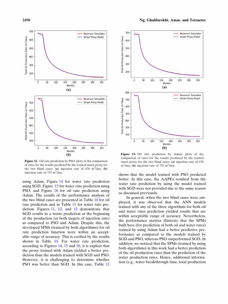
using Adam, Figure 14 for water rate predictionusing SGD, Figure 15 for water rate prediction usingPSO, and Figure 16 for oil rate prediction usingAdam. The results of the performance analysis ofthe two blind cases are presented in Table 10 for oilrate prediction and in Table 11 for water rate pre-diction. Figures 11, 12, and 13 demonstrate thatSGD results in a worse prediction at the beginningof the production (at both targets of injection rate)as compared to PSO and Adam. Despite this, thedeveloped SPMs (trained by both algorithms) for oilrate prediction function were within an accept-able range of accuracy. This is verified by the resultsshown in Table 10. For water rate prediction,according to Figures 14, 15 and 16, it is explicit thatthe proxy trained with Adam yielded a better pre-diction than the models trained with SGD and PSO.However, it is challenging to determine whetherPSO was better than SGD. In this case, Table 11

shows that the model trained with PSO predictedbetter. In this case, the AAPEs resulted from thewater rate prediction by using the model trainedwith SGD were not provided due to the same reasonas discussed previously.

In general, when the two blind cases were em-ployed, it was observed that the ANN modelstrained with any of the three algorithms for both oiland water rates prediction yielded results that arewithin acceptable range of accuracy. Nevertheless,the performance metrics illustrate that the SPMsbuilt here (for prediction of both oil and water rates)trained by using Adam had a better predictive per-formance as compared to the models trained bySGD and PSO, whereas PSO outperformed SGD. Inaddition, we noticed that the SPMs (trained by usingboth algorithms) in this work had a better predictionof the oil production rates than the prediction of thewater production rates. Hence, additional informa-tion (e.g., water breakthrough time, total production

Figure 12. Oil rate prediction by PSO: plots of the comparison

of rates for the results predicted by the trained smart proxy for

the two blind cases: (a) injection rate of 676 m3/day; (b)

injection rate of 755 m3/day.

Figure 13. Oil rate prediction by Adam: plots of the





of water) can be included as input data to improvethe performance of the SPM for water rate predic-tion.

After obtaining the flow rates predicted by thebuilt SPMs, we proceeded to the illustrative pro-duction optimization task. As briefly discussedabove, the optimization task here was to select thetarget of injection rate (between 676 m3/day and 755m3/day) that maximizes the objective function inEq. (23). By using Eqs. (23) and (24) along with theparameters listed in Table 2, the evolution of NPVthroughout the 30 years of production lifetime wasdetermined and is presented in Figure 17. The basecases shown in Figure 17 correspond to the cases forthe flow rates derived from the numerical reservoirsimulation to determine the evolution of NPV. Bothproxy models can reproduce the general trend of theNPV evolution that is close to the one generated bythe base cases. This observation is justifiable as all

the proxy models yielded the general trends of bothoil and water production rates as discussed earlier.Furthermore, from Table 12, all the models reachedto the same decision that having the target ofinjection rate to be 755 m3/day for 30 years (withouttermination of production during the period of30 years) will result in the maximum value of NPV.For the target rate of 676 m3/day, the percentageerror of the NPV resulted from the smart proxy ofSGD was about 2.67%, that of PSO was around1.41%, and that of Adam was about 0.61%. For thetarget rate of 755 m3/day, the percentage errors ofthe NPVs resulted from both proxy models of SGDand PSO were close, namely 1.38% for SGD and1.33% for PSO. However, for Adam, the percentageerror was approximately 0.43%. In this case, thesmart proxy trained by using Adam was deemedbetter. We understand that the economic modelused here might be insufficient to reflect the real-life

Figure 14. Water rate prediction by SGD: plots of the




Figure 15. Water rate prediction by PSO: plots of the





optimization case. However, we aimed to provideinsights regarding the use of SPMs in productionoptimization on a fundamental level.

We also provide a brief discussion on thecomputational time of these proxy models to high-light the advantage of applying them. The compu-tation here included all the training, validation,testing phases as well as the prediction using the twoblind cases. It was done by using a PC with config-

urations that included Intel� Core� i9-9900 [email protected] GHz with 64.0 GB RAM. Here, the compu-tation of one of the simulation scenarios listed inTable 3 took about 160 s to finish. When all the fivesimulation scenarios were run simultaneously, itspent about 290 s to be fully completed. Neverthe-less, for the SPM developed here, the computationtime of the proxy trained with SGD was about 110 s,that of PSO was about 50 s, and that of Adam wasabout 120 s.7 In this aspect, the computation of theproxy trained with backpropagation algorithm wasmore expensive than that of PSO because PSO is aderivative-free method. In general, we saw thatthere was still a noticeable (even not very signifi-cant) difference in the computational time betweenthe numerical simulation and the proxy models de-spite the low complexity of the reservoir model usedhere.

Further, we proposed and demonstrated theprobabilistic application to investigate further theoverall performance of the SPMs. In this case, one ofthe performance metrics, namely correlation coeffi-cient R2, was used for illustrative purpose in this partof the work. To do this probabilistic study of thebuilt SPMs, we conducted the process of SPM iter-atively for 200 times. This implies that there were200 samples of R2 for training phase, validationphase, testing phase, and prediction for each of thetwo blind cases. Thereafter, the normalized cumu-lative frequency distribution (NCFD) for R2 thatranged between 0 and 1 was computed for the 200samples. In this context, NCFD can be understoodas the cumulative number of times for a sample to bewithin a range of values of R2 over 200 times. Theplots of NCFD are presented in Figures 18, 19, 20,21, and 22.

Figure 16. Water rate prediction by Adam: plots of the




Table 10. Performance metrics of the smart proxy for the two

blind cases (oil rate prediction)

Injection

rate

AAPE

(%)

RMSE R2

Stochastic gradient

descent

676 m3/day 1.849 13.05 0.9924

755 m3/day 1.978 13.23 0.9932

Particle swarm opti-

mization

676 m3/day 1.391 5.701 0.9985

755 m3/day 0.708 5.695 0.9988

Adam 676 m3/day 0.999 2.501 0.9997

755 m3/day 1.057 2.830 0.9997

Table 11. Performance metrics of the smart proxy for the two

blind cases (water rate prediction)

Injection

rate

AAPE

(%)

RMSE R2

Stochastic gradient

descent

676 m3/day – 13.63 0.9917

755 m3/day 12.97 0.9935

Particle swarm opti-

mization

676 m3/day 8.623

7.266

8.454 0.9968

755 m3/day 8.975 0.9969

Adam 676 m3/day 8.049 2.790 0.9996

755 m3/day 7.061 4.385 0.9993

7 Computational time of the proxy built for oil rate prediction was

close to that of the proxy developed for water rate prediction.


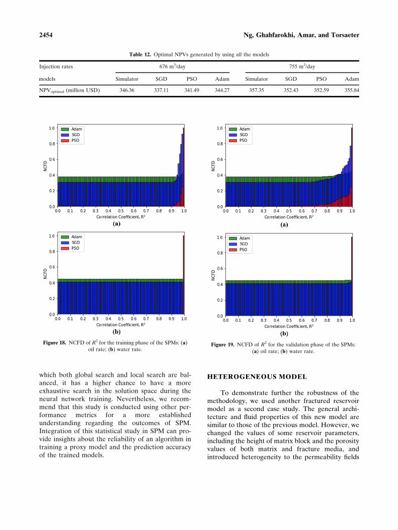
Based on Figure 18, for the training phase of theSPMs, the models trained with PSO had relativelyhigher chance to result in a healthy training trend

than the models trained with the backpropagationalgorithms. For the oil rate prediction, PSO had0.5% chance to result in values of R2 less than 0.90,whereas SGD had 31% chance and Adam had37.5% of chance. For the water rate prediction, PSOhad about 99% chance to yield values of R2 thatranged between 0.99 and 1, whereas SGD andAdam, respectively, had only about 60% and 55%chance to achieve that. According to these results,we deduced that PSO was more likely to produce ahealthy trend of training compared to SGD andAdam. This deduction is further justified by the re-sults shown in Figure 19 for the validation phase.

For the testing phase, it was noted that theproxy models trained by using PSO performed bet-ter that those of SGD and Adam when the modelswere evaluated against the testing dataset. As por-trayed in Figure 20, for the case of oil rate, there was26% chance that the model trained with PSO willproduce values of R2 less than 0.99 in the testingphase, whereas there was 76% chance that themodel trained with SGD will do so; for Adam, thechance was about 47%. Besides, for the case ofwater rate, PSO had 4% chance to have values of R2

less than 0.99, whereas SGD had 41.5% and Adamhad 45.5%. This provided more confidence that PSOhas a higher chance to yield a better predictiveperformance than SGD when the models were tes-ted with the dataset from a blind scenario.

For the prediction of rates against the datasetsfrom the two blind cases, it can be noticed that, ingeneral, the proxy models by PSO more likely had abetter predictive performance than those by SGDand Adam despite the fact that the former hadslightly higher chance to produce R2 values that areless than 0.90 compared with that SGD had in termsof oil rate prediction for injection scenario of676 m3/day. This is because based on the predictionof R2 that ranged between 0.99 and 1, the models byPSO were deemed more reliable than those by SGDand Adam. Besides, in terms of oil rate prediction,Adam statistically had a better chance than SGD inyielding R2 values between 0.99 and 1 for bothinjection scenarios. However, for water rate predic-tion, the chances of both algorithms were very close.We have illustrated that, here, statistically speaking,PSO had a better chance to perform better intraining and building the proxy model compared toSGD and Adam. Because PSO is metaheuristics, in

Figure 17. Evolution of NPV throughout the lifetime of

production: (a) SGD; (b) PSO; (c) Adam.


which both global search and local search are bal-anced, it has a higher chance to have a moreexhaustive search in the solution space during theneural network training. Nevertheless, we recom-mend that this study is conducted using other per-formance metrics for a more establishedunderstanding regarding the outcomes of SPM.Integration of this statistical study in SPM can pro-vide insights about the reliability of an algorithm intraining a proxy model and the prediction accuracyof the trained models.

HETEROGENEOUS MODEL

To demonstrate further the robustness of themethodology, we used another fractured reservoirmodel as a second case study. The general archi-tecture and fluid properties of this new model aresimilar to those of the previous model. However, wechanged the values of some reservoir parameters,including the height of matrix block and the porosityvalues of both matrix and fracture media, andintroduced heterogeneity to the permeability fields

Table 12. Optimal NPVs generated by using all the models

Injection rates 676 m3/day 755 m3/day

models Simulator SGD PSO Adam Simulator SGD PSO Adam

NPVoptimal (million USD) 346.36 337.11 341.49 344.27 357.35 352.43 352.59 355.84

Figure 18. NCFD of R2 for the training phase of the SPMs: (a)

oil rate; (b) water rate.Figure 19. NCFD of R2 for the validation phase of the SPMs:

(a) oil rate; (b) water rate.


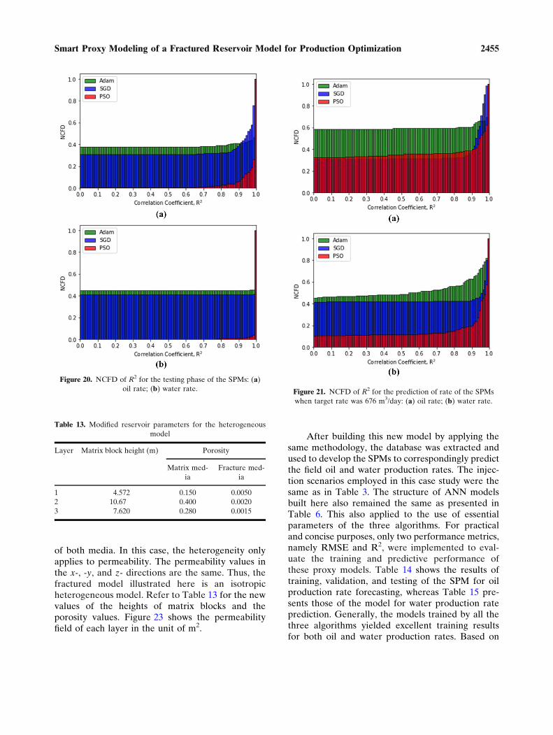
of both media. In this case, the heterogeneity onlyapplies to permeability. The permeability values inthe x-, -y, and z- directions are the same. Thus, thefractured model illustrated here is an isotropicheterogeneous model. Refer to Table 13 for the newvalues of the heights of matrix blocks and theporosity values. Figure 23 shows the permeabilityfield of each layer in the unit of m2.

After building this new model by applying thesame methodology, the database was extracted andused to develop the SPMs to correspondingly predictthe field oil and water production rates. The injec-tion scenarios employed in this case study were thesame as in Table 3. The structure of ANN modelsbuilt here also remained the same as presented inTable 6. This also applied to the use of essentialparameters of the three algorithms. For practicaland concise purposes, only two performance metrics,namely RMSE and R2, were implemented to eval-uate the training and predictive performance ofthese proxy models. Table 14 shows the results oftraining, validation, and testing of the SPM for oilproduction rate forecasting, whereas Table 15 pre-sents those of the model for water production rateprediction. Generally, the models trained by all thethree algorithms yielded excellent training resultsfor both oil and water production rates. Based on

Table 13. Modified reservoir parameters for the heterogeneous

model

Layer Matrix block height (m) Porosity

Matrix med-

ia

Fracture med-

ia

1 4.572 0.150 0.0050

2 10.67 0.400 0.0020

3 7.620 0.280 0.0015

Figure 21. NCFD of R2 for the prediction of rate of the SPMs

when target rate was 676 m3/day: (a) oil rate; (b) water rate.

Figure 20. NCFD of R2 for the testing phase of the SPMs: (a)oil rate; (b) water rate.


both RMSE and R2, Adam had the best results forboth oil and water production rates. Nevertheless,for the testing phase in oil rate proxy model, PSOoutperformed the others. For illustrative purposes,only the production profiles estimated by the smartproxies trained by using Adam are presented; the oilprofiles are shown in Figure 24, whereas the waterprofiles are presented in Figure 25.

Thereafter, these models also underwent theblind validation phases by using the two blind casesas explained before. Table 16 records the results ofblind validation for oil rate prediction, and Table 17shows the results for water rate forecasting. For thiscase study, the PSO outperformed the others when itwas used to train the predictive model of oil pro-duction rate. However, for the estimation of waterproduction rate, Adam still yielded the predictivemodel that produced the best results. Then, theproduction optimization was also done by using the

same price setting as shown in Table 2 to highlightthe fundamental practicality of the models devel-oped in this case study. The optimal NPVs obtainedby using each of the proxy models are tabulated inTable 18.

Based on Table 18, it was deduced that theproxy models built by using Adam produced theoptimal NPV with the least percentage error undertwo different injection scenarios, which were 0.117%for injection rate of 676 m3/day and 0.329% forinjection rate of 755 m3/day. In addition, all theproxy models reached the same option that theinjection rate of 755 m3/day was economicallypreferable. Apart from these, for illustrative andsuccinct purposes, the probabilistic application wasonly implemented to analyze the predictive perfor-mance of each model. The results of this applicationare demonstrated in Figure 26 for the target rate of676 m3/day and in Figure 27 for the target rate of755 m3/day. In general, for this case study, it can be

Table 14. Performance metrics of the smart proxy for oil rate

prediction based on training, validation, and testing sets

RMSE R2

Stochastic gradient des-

cent

Training (758 data) 7.855 0.9977

Validation (163

data)

4.700 0.9992

Testing (162 data) 8.202 0.9978

Particle swarm optimiza-

tion

Training (758 data) 3.846 0.9995

Validation (163

data)

3.918 0.9995

Testing (162 data) 2.739 0.9997

Adam Training (758 data) 3.154 0.9997

Validation (163

data)

2.410 0.9998

Testing (162 data) 3.391 0.9996

Table 15. Performance metrics of the smart proxy for water rate

prediction based on training, validation, and testing sets

RMSE R2

Stochastic gradient des-

cent

Training (758 data) 2.401 0.9998

Validation (163

data)

2.273 0.9998

Testing (162 data) 2.379 0.9998

Particle swarm optimiza-

tion

Training (758 data) 1.869 0.9999

Validation (163

data)

1.961 0.9999

Testing (162 data) 1.824 0.9999

Adam Training (758 data) 0.540 0.9999

Validation (163

data)

0.478 0.9999

Testing (162 data) 0.422 0.9999




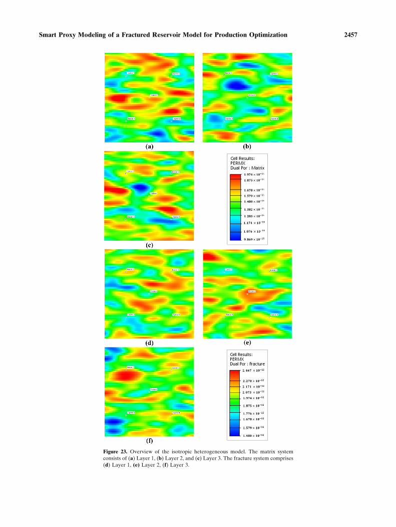
Figure 23. Overview of the isotropic heterogeneous model. The matrix system

consists of (a) Layer 1, (b) Layer 2, and (c) Layer 3. The fracture system comprises

(d) Layer 1, (e) Layer 2, (f) Layer 3.


deduced that PSO had a better chance than bothSGD and Adam to produce a predictive model withhigher accuracy level (i.e., R2 exceeding 0.99).

CONCLUSIONS

Here, we have shown how SPM can be con-ducted by using a synthetic fractured reservoir

model. The purpose of this study was to providesome insights and a more concrete demonstrationregarding the modeling of a smart proxy. We alsobriefly discussed how the spatio-temporal databasecan be generated, and we presented the selection ofinput and output data which were used in the neuralnetwork training. This procedure is of paramountimportance as a good database determines the suc-cess of SPM. Apart from implementing the back-

Table 16. Oil rate prediction: performance metrics of the smart proxy for the two blind cases

Injection rate RMSE R2

Stochastic gradient descent 676 m3/day 12.45 0.9939

755 m3/day 13.04 0.9944

Particle Swarm Optimization 676 m3/day 2.097 0.9998

755 m3/day 3.827 0.9995

Adam 676 m3/day 4.489 0.9992

755 m3/day 5.468 0.9990

Figure 24. Oil rate prediction by Adam: plots of the results

predicted by the trained smart proxy for the two blind cases:

(a) injection rate of 676 m3/day; (b) injection rate of 755

m3/day.

Figure 25. Water rate prediction by Adam: plots of the results

predicted by the trained smart proxy for the two blind cases:

(a) injection rate of 676 m3/day; (b) injection rate of 755

m3/day.


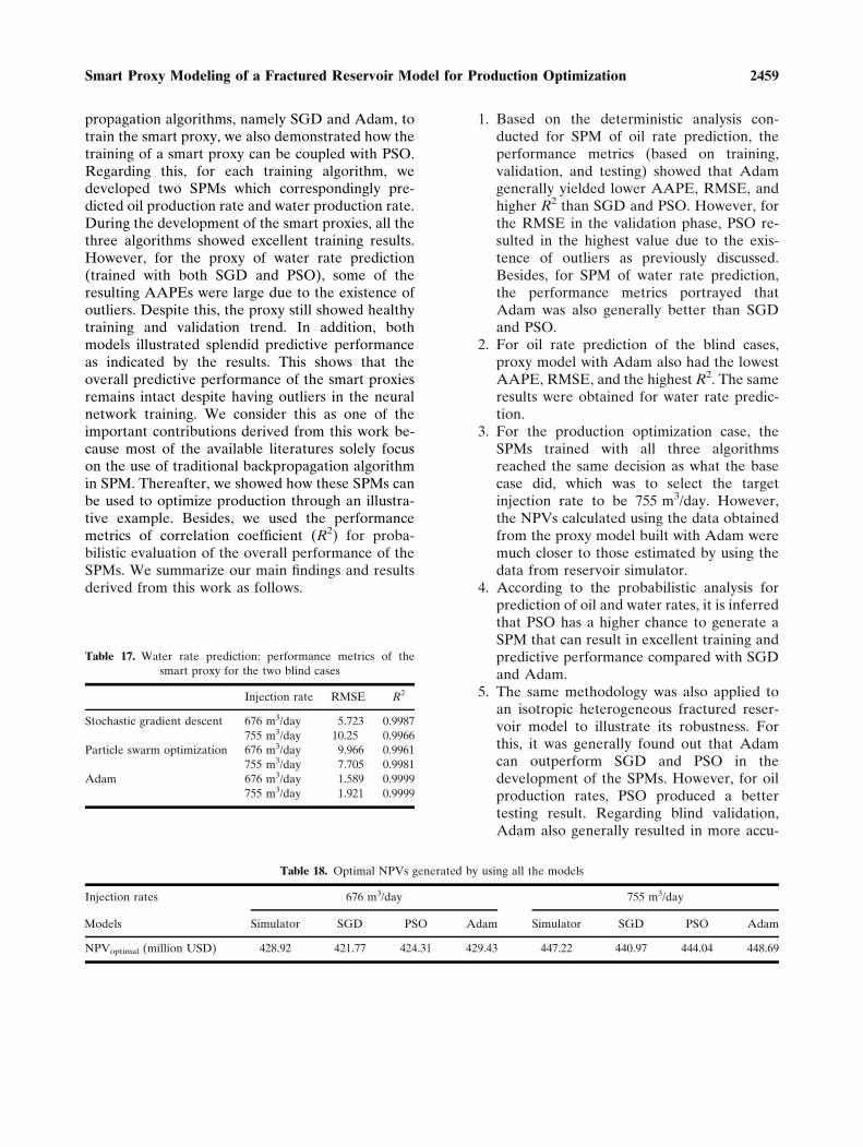
propagation algorithms, namely SGD and Adam, totrain the smart proxy, we also demonstrated how thetraining of a smart proxy can be coupled with PSO.Regarding this, for each training algorithm, wedeveloped two SPMs which correspondingly pre-dicted oil production rate and water production rate.During the development of the smart proxies, all thethree algorithms showed excellent training results.However, for the proxy of water rate prediction(trained with both SGD and PSO), some of theresulting AAPEs were large due to the existence ofoutliers. Despite this, the proxy still showed healthytraining and validation trend. In addition, bothmodels illustrated splendid predictive performanceas indicated by the results. This shows that theoverall predictive performance of the smart proxiesremains intact despite having outliers in the neuralnetwork training. We consider this as one of theimportant contributions derived from this work be-cause most of the available literatures solely focuson the use of traditional backpropagation algorithmin SPM. Thereafter, we showed how these SPMs canbe used to optimize production through an illustra-tive example. Besides, we used the performancemetrics of correlation coefficient (R2) for proba-bilistic evaluation of the overall performance of theSPMs. We summarize our main findings and resultsderived from this work as follows.

1. Based on the deterministic analysis con-ducted for SPM of oil rate prediction, theperformance metrics (based on training,validation, and testing) showed that Adamgenerally yielded lower AAPE, RMSE, andhigher R2 than SGD and PSO. However, forthe RMSE in the validation phase, PSO re-sulted in the highest value due to the exis-tence of outliers as previously discussed.Besides, for SPM of water rate prediction,the performance metrics portrayed thatAdam was also generally better than SGDand PSO.

2. For oil rate prediction of the blind cases,proxy model with Adam also had the lowestAAPE, RMSE, and the highest R2. The sameresults were obtained for water rate predic-tion.

3. For the production optimization case, theSPMs trained with all three algorithmsreached the same decision as what the basecase did, which was to select the targetinjection rate to be 755 m3/day. However,the NPVs calculated using the data obtainedfrom the proxy model built with Adam weremuch closer to those estimated by using thedata from reservoir simulator.

4. According to the probabilistic analysis forprediction of oil and water rates, it is inferredthat PSO has a higher chance to generate aSPM that can result in excellent training andpredictive performance compared with SGDand Adam.

5. The same methodology was also applied toan isotropic heterogeneous fractured reser-voir model to illustrate its robustness. Forthis, it was generally found out that Adamcan outperform SGD and PSO in thedevelopment of the SPMs. However, for oilproduction rates, PSO produced a bettertesting result. Regarding blind validation,Adam also generally resulted in more accu-

Table 17. Water rate prediction: performance metrics of the

smart proxy for the two blind cases

Injection rate RMSE R2

Stochastic gradient descent 676 m3/day 5.723 0.9987

755 m3/day 10.25 0.9966

Particle swarm optimization 676 m3/day 9.966 0.9961

755 m3/day 7.705 0.9981

Adam 676 m3/day 1.589 0.9999

755 m3/day 1.921 0.9999

Table 18. Optimal NPVs generated by using all the models

Injection rates 676 m3/day 755 m3/day

Models Simulator SGD PSO Adam Simulator SGD PSO Adam

NPVoptimal (million USD) 428.92 421.77 424.31 429.43 447.22 440.97 444.04 448.69


rate predictive models of water productionrates. Nonetheless, the predictive model ofoil rates established by using PSO estimatedthe oil profile more accurately. Additionally,PSO showed higher chance than SGD andAdam to produce models with excellentpredictive ability.

Based on the findings presented, we concludethat, in this work, a metaheuristic algorithm can beapplied aptly to train and build a good smart proxyof a fractured reservoir model. Although it has beendemonstrated that PSO might not deterministicallyoutperform the considered backpropagation algo-rithms in smart proxy modeling, statistically it stillhas a better chance to yield a good performance inthis case study. Nonetheless, we understand thatthere are still some shortcomings regarding theseSPMs. We hope that these proxies can be enhanced

to be more tractable and robust8 in terms of pre-diction of any reservoir-related parameter. In short,we believe that we have achieved the main goals ofthis work, which include a vivid illustration of SPM,an integration of metaheuristic algorithm in proxytraining, a presentation of practical use of the builtproxies in optimization on a fundamental level, andan inclusion of a probabilistic application in evalu-ating a proxy model.

ACKNOWLEDGMENTS

This research is a part of BRU21 – NTNUResearch and Innovation Program on DigitalAutomation Solutions for the Oil and Gas Industry(www.ntnu.edu/bru21). The authors would also like




when target rate was 755 m3/day: (a) Oil rate� (b) Water rate.

8 ‘‘Robust’’ here implies that the smart proxy model can be used

in real-life cases.


http://www.ntnu.edu/bru21

to acknowledge the support given by the Depart-ment of Geoscience and Petroleum (IGP) of NTNUto this research work.

OPEN ACCESS

This article is licensed under a Creative Com-mons Attribution 4.0 International License, whichpermits use, sharing, adaptation, distribution andreproduction in any medium or format, as long asyou give appropriate credit to the original author(s)and the source, provide a link to the CreativeCommons licence, and indicate if changes weremade. The images or other third party material inthis article are included in the article’s CreativeCommons licence, unless indicated otherwise in acredit line to the material. If material is not includedin the article’s Creative Commons licence and yourintended use is not permitted by statutory regulationor exceeds the permitted use, you will need to obtainpermission directly from the copyright holder. Toview a copy of this licence, visit http://creativecommons.org/licenses/by/4.0/.

FUNDING

Open access funding provided by NTNU Nor-wegian University of Science and Technology (inclSt. Olavs Hospital - Trondheim University Hospi-tal).!/FundingInformation>

REFERENCES

Ahmad, S. A., & Olivier, R. G. (2008). Matrix-fracture transferfunction in dual-medium flow simulation: review, compar-ison, and validation. In Europec/EAGE Conference andExhibition. Rome, Italy. https://doi.org/https://doi.org/10.2118/113890-MS.

Alenezi, F., & Mohaghegh, S. D. (2016). A data-driven smartproxy model for a comprehensive reservoirsimulation. In The4th Saudi International Conference on Information Technol-ogy (Big Data Analysis) (KACSTIT). Riyadh, Saudi Arabia.https://doi.org/10.1109/KACSTIT.2016.7756063.

Alenezi, F., & Mohaghegh, S. D. (2017). Developing a smartproxy for the SACROC water-flooding numerical reservoirsimulation model. In SPE Western Regional Meeting. Bak-ersfield, California, United States. https://doi.org/https://doi.org/10.2118/185691-MS.

Barrenblatt, G. I., Zheltov, I. P., & Kochina, I. N. (1960). Basicconcepts in the theory of homogeneous liquids in fissured

rocks. Journal of Applied Mathematics and Mechanics, 24(5),1286–1303.

Bianchi, L., Dorigo, M., Gambardella, L. M., & Gutjahr, W. J.(2009). A survey on metaheuristics for stochastic combina-torial optimization. Natural Computing, 8, 239–287.

British Petroleum. (2020). BP Statistical Review of World Energy2020. https://www.bp.com/en/global/corporate/energy-economics/statistical-review-of-world-energy.html. Retrieved July21, 2020.

Buduma, N., & Locasio, N. (2017). Fundamentals of deep learning:Designing next-generation machine intelligence algorithms.Sebastopol, California, United States: O�Reilly.

Ceetron Solution AS. (2020). ResInsight.Chollet, F. (2019). Keras, version 2.3.0.Ertekin, T., & Sun, Q. (2019). Artificial intelligence applications

in reservoir engineering: A status check. Energies, 12(15),2897.

Firoozabadi, A., & Thomas, L. K. (1990). Sixth SPE comparativesolution project: Dual-porosity simulators. Journal of Petro-leum Technology, 42(6), 710–715.

Gerald, P., Raftley, A. E., Sevcıkova, H., Li, N., Gu, D.,Spoorenberg, T., et al. (2014). World population stabilizationunlikely this century. Science, 346(6206), 234–237.

Gharbi, R. B. C., & Mansoori, G. A. (2005). An introduction toartificial intelligence applications in petroleum explorationand production. Journal of Petroleum Science and Engineer-ing, 49(3–4), 93–96.

Gilman, J. R., & Kazemi, H. (1983). Improvements in simulationof naturally fractured reservoirs. Society of Petroleum Engi-neers Journal, 23(4), 695–707.

Google Brain Team. (2020). TensorFlow, version 2.1.0.He, Q., Mohaghegh, S. D., & Liu, Z. (2016). Reservoir simulation

using smart proxy in SACROC unit—case study. 2016. InSPE Eastern Regional Meeting. Canton, Ohio, United States.https://doi.org/https://doi.org/10.2118/184069-MS.

International Energy Agency. (2018). World Energy Outlook2018. International Energy Agency. https://www.iea.org/weo2018/. Retrieved September 24, 2019.

Kazemi, H., Merrill, L. S., Jr., Porterfield, K. L., & Zeman, P. R.(1976). Numerical simulation of water-oil flow in naturallyfractured reservoirs. Society of Petroleum Engineers Journal,16(6), 317–326.

Kennedy, J., & Eberhart, R. (1995). Particle Swarm Optimization.In IEEE International Conference on Neural Networks.Perth, Western Australia, Australia. https://doi.org/10.1109/ICNN.1995.488968.

Kingma, D. P., & Ba, J. (2015). Adam: A method for stochasticoptimization. In The 3rd International Conference forLearning Representations. San Diego, California, UnitedStates. arxiv.org/abs/1412.6980.

Lescaroux, F., & Mignon, V. (2009). On the influence of oil priceson economic activity and other macroeconomic and financialvariables. OPEC Energy Review, 32(4), 343–380.

Mohaghegh, S. D. (2000a). Virtual Intelligence applications inpetroleum engineering: Part 1—artificial neural networks.Journal of Petroleum Technology, 52(9), 64–72.

Mohaghegh, S. D. (2000b). Virtual intelligence applications inpetroleum engineering: Part 2—evolutionary computing.Journal of Petroleum Technology, 52(10), 40–46.

Mohaghegh, S. D. (2000c). Virtual intelligence applications inpetroleum engineering: Part 3—fuzzy logic. Journal of Pet-roleum Technology, 52(11), 82–87.

Mohaghegh, S. D., Modavi, C. A., Hafez, H. H., Haajizadeh, M.,Kenawy, M.M., & Guruswamy, S. (2006). Development ofsurrogate reservoir models (SRM) for fast track analysis ofcomplex reservoirs. In Intelligent Energy Conference andExhibition. Amsterdam, The Netherlands. https://doi.org/https://doi.org/10.2118/99667-MS.


http://creativecommons.org/licenses/by/4.0/

http://creativecommons.org/licenses/by/4.0/

https://doi.org/10.2118/113890-MS

https://doi.org/10.2118/113890-MS

https://doi.org/10.1109/KACSTIT.2016.7756063

https://doi.org/10.2118/185691-MS

https://doi.org/10.2118/185691-MS

https://www.bp.com/en/global/corporate/energy-economics/statistical-review-of-world-energy.html

https://www.bp.com/en/global/corporate/energy-economics/statistical-review-of-world-energy.html

https://doi.org/10.2118/184069-MS

https://www.iea.org/weo2018/

https://www.iea.org/weo2018/

https://doi.org/10.1109/ICNN.1995.488968

https://doi.org/10.1109/ICNN.1995.488968

https://doi.org/10.2118/99667-MS


Mohaghegh, S. D. (2011). Reservoir simulation and modelingbased on pattern recognition. In SPE Digital Energy Con-ference and Exhibition. The Woodlands, Texas, USA.https://doi.org/https://doi.org/10.2118/143179-MS.

Mohaghegh, S. D., Liu, J. S., Gaskari, R., Mayasami, M., &Olukoko, O. A. (2012a). Application of surrogate reservoirmodels (SRM) to an onshore green field in Saudi Arabia;Case Study. In North Africa Technical Conference andExhibition. Cairo, Egypt. https://doi.org/https://doi.org/10.2118/151994-MS.

Mohaghegh, S. D., Amini, S., Gholami, V., Gaskari, R., &Bromhal, G. S. (2012b). Grid-based surrogate reservoirmodeling (SRM) for fast track analysis of numerical reservoirsimulation models at the gridblock level. In SPE WesternRegional Meeting. Bakersfield, California, United States.https://doi.org/https://doi.org/10.2118/153844-MS.

Mohaghegh, S. D., Liu, J. S., Gaskari, R., Mayasami, M., &Olukoko, O. A. (2012c). Application of surrogate reservoirmodels (SRM) to Two offshore fields in Saudi Arabia; CaseStudy. In SPE Western Regional Meeting. Bakersfield, Cali-fornia, United States. https://doi.org/https://doi.org/10.2118/153845-MS.

Mohaghegh, S. D., Abdulla, F., Abdou, M., Gaskari, R., &Mayasami, M. (2015). Smart proxy: An innovative reservoirmanagement tool; Case study of a giant mature oilfield in theUAE. In Abu Dhabi International Petroleum Exhibition andConference. Abu Dhabi, UAE. https://doi.org/https://doi.org/10.2118/177829-MS.

Mohaghegh, S. D. (2017). Data-Driven Reservoir Modeling.Richardson, Texas, United States: Society of PetroleumEngineers.

Mohaghegh, S. D. (2018). Data-driven analytics for the geologicalstorage of CO2. Boca Raton, Florida, United States: CRCPress.

Miranda, L. J. V. (2019). PySwarms, version 1.1.0.Nait Amar, M., Zeraibi, N., & Redouane, K. (2018). Bottom hole

pressure estimation using hybridization neural networks andgrey wolves optimization. Petroleum, 4(4), 419–429.

Nait Amar, M., Zeraibi, N., & Redouane, K. (2018). Pure CO2-oilsystem miscibility pressure prediction using optimized neuralnetwork by differential evolution. Petroleum and Coal, 60(2),284–293.

Nait Amar, M., & Jahanbani Ghahfarokhi, A. (2020). Predictionof CO2 diffusivity in brine using white-box machine learning.Journal of Petroleum Science and Engineering, 190, 107037.

Nait Amar, M., Zeraibi, N., & Jahanbani Ghahfarokhi, A. (2020).Applying hybrid support vector regression and genetic algo-rithm to water alternating CO2 gas EOR. Greenhouse Gases:Science and Technology, 10(3), 613–630.

Parada, C. H., & Ertekin, T. (2012). A New screening tool forimproved oil recovery methods using artificial neural net-works. In SPE Western Regional Meeting. Bakersfield, Cali-fornia, United States. https://doi.org/https://doi.org/10.2118/153321-MS.

Python Software Foundation. (2020). Python version 3.8.1..Romm, E. S. (1966). Fluid flow in fractured rocks. Moscow,

Russia: Nedra Publishing House. (in Russian).Schlumberger. (2020a). ECLIPSE 100 Reservoir Engineering

Software.Schlumberger. (2020b). Technical Challenges - Carbonate

Reservoirs; https://www.slb.com/technical-challenges/carbonates.

Shi, Y., & Eberhart, R. (1998). A modified particle swarm opti-mizer. In IEEE International Conference on EvolutionaryComputation Proceedings. IEEE World Congress on Com-putational Intelligence (Cat. No.98TH8360). Anchorage,Alaska, United States. https://doi.org/10.1109/ICEC.1998.699146.

Shi, Y., & Eberhart, R. (1999). Empirical study of particle swarmoptimization. In Proceedings of the 1999 Congress on Evo-lutionary Computation-CEC99 (Cat. No. 99TH8406). Wash-ington DC, United States. https://doi.org/10.1109/CEC.1999.785511.

Su, S., Gosselin, O., Parvizi, H., and Giddins, M. A. (2013). Dy-namic matrix-fracture transfer behavior in dual-porositymodels. In EAGE Annual Conference and Exhibition incor-porating SPE Europec. London, UK. https://doi.org/https://doi.org/10.2118/164855-MS.

Uleberg, K., & Kleppe, J. (1996). Dual porosity, dual permeabilityformulation for fractured reservoir simulation. In RUTHSeminar. Stavanger, Norway. http://www.ipt.ntnu.no/�kleppe/TPG4150/fracturedpaper.pdf.

Van Golf-Racht, T. D. (1982). Fundamentals of fractured reservoirengineering. New York, United States: Elsevier Scientific.

Warren, J. E., & Root, P. J. (1963). The behavior of naturallyfractured reservoirs. Society of Petroleum Engineers Journal,3(3), 245–255.

Wiggins, M. L., & Startzman, R. A. (1990). An approach toreservoir management. In SPE Annual Technical Conferenceand Exhibition 1990. New Orleans, Louisiana, USA.https://doi.org/https://doi.org/10.2118/20747-MS.

Wilamowski, B. M., & Irwin, J. D. (2011). The industrial elec-tronics handbook second edition: Intelligent system. BocaRaton, Florida, United States: CRC Press.

Zhang, Y., Wang, S., & Ji, G. (2015). A comprehensive survey onparticle swarm optimization algorithm and its applications.Mathematical Problems in Engineering, 2015, 1–38.


https://doi.org/10.2118/143179-MS

https://doi.org/10.2118/151994-MS

https://doi.org/10.2118/151994-MS

https://doi.org/10.2118/153844-MS

https://doi.org/10.2118/153845-MS

https://doi.org/10.2118/153845-MS

https://doi.org/10.2118/177829-MS

https://doi.org/10.2118/177829-MS

https://doi.org/10.2118/153321-MS

https://doi.org/10.2118/153321-MS

https://www.slb.com/technical-challenges/carbonates

https://www.slb.com/technical-challenges/carbonates

https://doi.org/10.1109/ICEC.1998.699146

https://doi.org/10.1109/ICEC.1998.699146

https://doi.org/10.1109/CEC.1999.785511

https://doi.org/10.1109/CEC.1999.785511

https://doi.org/10.2118/164855-MS

https://doi.org/10.2118/164855-MS

http://www.ipt.ntnu.no/~kleppe/TPG4150/fracturedpaper.pdf




Smart Proxy Modeling of a Fractured Reservoir Model for ...

Documents

Transcript of Smart Proxy Modeling of a Fractured Reservoir Model for ...