Smart Dispatch and Demand Forecasting for Large Grid Operations

4

Smart Dispatch and Demand Forecasting for Large Grid Operations with Integrated

Renewable Resources

Kwok W. Cheung Alstom Grid Inc.

USA

1. Introduction

The restructured electric power industry has brought new challenges and concerns for the secured operation of stressed power systems. As renewable energy resources, distributed generation, and demand response become significant portions of overall generation resource mix, smarter or more intelligent system dispatch technology is needed to cope with new categories of uncertainty associated with those new energy resources. The need for a new dispatch system to better handle the uncertainty introduced by the increasing number of new energy resources becomes more and more inevitable. In North America, almost all Regional Transmission Organizations (RTO) such as PJM, Midwest ISO, ISO New England, California ISO or ERCOT, are fundamentally reliant on wholesale market mechanism to optimally dispatch energy and ancillary services of generation resources to reliably serve the load in large geographical regions. Traditionally, the real-time dispatch problem is solved as a linear programming or a mixed integer programming problem assuming absolute certainty of system input parameters and there is very little account of system robustness other than classical system reserve modeling. The next generation of dispatch system is being designed to provide dispatchers with the capability to manage uncertainty of power systems more explicitly. The uncertainty of generation requirements for maintaining system balancing has been

growing significantly due to the penetration of renewable energy resources such as wind

power. To deal with such uncertainty, RTO’s require not only more accurate demand

forecasting for longer-term prediction beyond real-time, but also demand forecasting with

confidence intervals.

This chapter addresses the challenges of smart grid from a generation dispatch

perspective. Various aspects of integration of renewable resources to power grids will be

discussed. The framework of Smart Dispatch will be proposed. This chapter highlights

some advanced demand forecasting techniques such as wavelet transform and composite

forecasting for more accurate demand forecasting that takes renewable forecasting into

consideration. A new dispatch system to provide system operators with look-ahead

capability and robust dispatch solution to cope with uncertain intermittent resources is

presented.

www.intechopen.com

Renewable Energy – Trends and Applications 76

2. Challenges of smart grid

In recent years, energy systems whether in developed or emerging economies are undergoing changes due to the emphasis of renewable resources. This is leading to a profound transition from the current centralized infrastructure towards the massive introduction of distributed generation, responsive/controllable demand and active network management throughout the smart grid ecosystem as shown in Figure 1. Unlike conventional generation resources, outputs of many of renewable resources do not follow traditional generation/load correlation but have strong dependencies on weather conditions, which from a system prospective are posing new challenges associated with the monitoring and controllability of the demand-supply balance. As distributed generations, demand response and renewable energy resources become significant portions of overall system installed capacity, a smarter dispatch system for generation resources is required to cope with the new uncertainties being introduced by the new resources. One method to cope with uncertainties is to create a better predictive model (Cheung et al., 2010, 2009). This includes better modeling of transmission constraints, better modeling of resource characteristics including capacity limits and ramp rates, more accurate demand forecasting and external transaction schedule forecasting that ultimately result in a more accurate prediction of generation pattern and system conditions. Another method to cope with uncertainties is to address the robustness of dispatch solutions (Rios-Zalapa et al., 2010). Optimality or even feasibility of dispatch solutions could be very sensitive to system uncertainties. Reserve requirements and “n-1” contingency analysis are traditional ways to ensure certain robustness of a given system. Scenario-based (Monte-Carlo) simulation is another common technique for assessing economic or reliability impact with respect to uncertainties such as renewable energy forecast. These methods and techniques are necessary as the industry integrates renewable energy resources into the power grid.

2.1 Renewable energy grid integration Like any other form of generation, renewable resources such as wind or solar power will

have an impact on power system reserves and will also contribute to a reduction in fuel

usage and emissions. In particular, the impact of wind power not only depends on the wind

power penetration level, but also on the power system size, geographical area, generation

capacity mix, the degree of interconnection to neighboring systems and load variations.

Some of the major challenges of renewable energy integration need to be addressed in the

following main areas:

Design and operation of the power system

Grid infrastructure

Connection requirements for renewable power plants

System adequacy and the security of supply

Electricity market design With increasing penetration and reliance on renewable resources have come heightened operational concerns over maintaining system balance. Ancillary services, such as operating reserves, imbalance energy, and frequency regulation, are necessary to support renewable energy integration, particularly the integration of intermittent resources (Chuang & Schwaegerl, 2009). Without supporting ancillary services, increased risk to system imbalance is introduced by the uncertainty of renewable generation availability, especially in systems with significant penetration of resources powered by intermittent supply, such as wind and solar.

www.intechopen.com

Smart Dispatch and Demand Forecasting for Large Grid Operations with Integrated Renewable Resources 77

For the purposes of balancing, the qualities of wind energy must be analyzed in a directly comparable way to that adopted for conventional plants. Balancing solutions involve mostly existing conventional generation units (thermal and hydro). In future developments of power systems, increased flexibility should be encouraged as a major design principle (flexible generation, demand side management, interconnections, storage etc.), in order to manage the increased variability induced by renewable resources. Market design issues such as gate-closure times should be reduced for variable output technologies. The real-time or balance market rules must be adjusted to improve accuracy of forecasts and enable temporal and spatial aggregation of wind power output forecasts. Curtailment of wind power production should be managed according to least-cost principles from an overall system point of view.

Fig. 1. Smart Grid Ecosystem

www.intechopen.com


3. Smart dispatch of generation resources

Smart dispatch (SD) represents a new era of economic dispatch. In general, economic dispatch is about the operation of generation facilities to produce energy at the lowest cost to reliably serve consumers, recognizing any operational limits of generation and transmission facilities. The problem of economic dispatch and its solutions have evolved over the years.

3.1 Evolution of economic dispatch The evolution timeline of economic dispatch could be divided into the following three major periods: 1. Classical dispatch [1970’s – 1990’s] (Wood & Wollenberg, 1996) 2. Market-based dispatch [1990’s – 2010’s] (Schweppe et al., 1998; Ma et al., 1999; Chow et

al., 2005) 3. Smart dispatch [2010’s – ] (Cheung et al., 2009)

3.1.1 Classical dispatch Since the birth of control center’s energy management system, classical dispatch monitors

load, generation and interchange (imports/exports) to ensure balance of supply and

demand. It also maintains system frequency during dispatch according to some regulatory

standards, using Automatic Generation Control (AGC) to change generation dispatch as

needed. It monitors hourly dispatch schedules to ensure that dispatch for the next hour will

be in balance. Classical dispatch also monitors flows on transmission system. It keeps

transmission flows within reliability limits, keeps voltage levels within reliability ranges and

takes corrective action, when needed, by limiting new power flow schedules, curtailing

existing power flow schedules, changing the dispatch or shedding load. The latter set of

monitoring and control functions is typically performed by the transmission operator.

Traditionally, generation scheduling/dispatch and grid security are separate independent

tasks within control centers. Other than some ad hoc analysis, classical dispatch typical only

addresses the real-time condition without much consideration of scenarios in the past or the

future.

3.1.2 Market-based dispatch Ensuring reliability of the physical power system is no longer the only responsibility for the

RTO/ISOs. A lot of the RTOs/ISOs are also responsible for operating wholesale electricity

markets. An electricity market in which the ISO or RTO functions both as the “system

operator” for reliability coordination and the “market operator” for establishing market

prices allows commercial freedom and centralized economic and reliability coordination to

co-exist harmoniously (Figure 2). To facilitate market transparency and to ensure reliability

of the physical power system, an optimization-based framework is used to provide an

Taking advantage of the mathematical rigor contained in formal optimization methodology,

the rules are likely to be more consistent, and thus more defensible against challenges that

effective context for defining comprehensive rules for scheduling, pricing, and dispatching.

invariably arise in any market.

Congestion management via the mechanism of locational marginal pricing (LMP) becomes an integral part of design of many wholesale electricity markets throughout the world and

www.intechopen.com


security-constrained economic dispatch (SCED) becomes a critical application to ensure the transmission constraints are respected while generation resources are being dispatched economically. The other important aspect of market-based dispatch is the size of the dispatch system. A typical system like PJM or Midwest ISO is usually more than 100GW of installed capacity. Advances in mathematical algorithms and computer technology really make the near real-time dispatch and commitment decisions a reality.

Fig. 2. Dual functions of RTO/ISO and dual solutions of SCED

3.1.3 Smart dispatch Smart dispatch (SD) is envisioned to be the next generation of resource dispatch solution particularly designed for operating in the smart grid environment (Cheung et al., 2009). The “smartness” of this new era of dispatch is to be able to manage highly distributed and active generation/demand resources in a direct or indirect manner. With the introduction of distributed energy resources such as renewable generations, PHEVs (Plug-in Hybrid Electric Vehicles) and demand response, the power grid will need to face the extra challenges in the following areas:

Energy balancing

Reliability assessment

Renewable generation forecasting

Demand forecasting

Ancillary services procurement

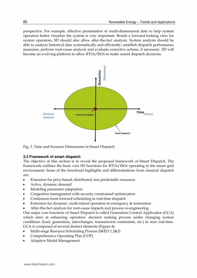
Distributed energy resource modeling A lot of the new challenges are due to the uncertainties associated with the new resources/devices that will ultimately impact both system reliability and power economics. When compared to the classical dispatch which only deals with a particular scenario for a single time point, smart dispatch addresses a spectrum of scenarios for a specified time period (Figure 3). Thus the expansion in time and scenarios for SD makes the problem of SD itself pretty challenging from both a computational perspective and a user interface

SystemOperator

MarketOperator

NetworkModel and

Constraints

LoadForecast

BalancedDispatch

Points

Bid DataMarketPrices

RTO/ISO

DualSolutionsof SCED

www.intechopen.com


perspective. For example, effective presentation of multi-dimensional data to help system operators better visualize the system is very important. Beside a forward-looking view for system operators, SD should also allow after-the-fact analysis. System analysts should be able to analyze historical data systematically and efficiently, establish dispatch performance measures, perform root-cause analysis and evaluate corrective actions, if necessary. SD will become an evolving platform to allow RTOs/ISOs to make sound dispatch decisions.

Fig. 3. Time and Scenario Dimensions in Smart Dispatch

3.2 Framework of smart dispatch The objective of this section is to reveal the proposed framework of Smart Dispatch. The framework outlines the basic core SD functions for RTOs/ISOs operating in the smart grid environment. Some of the functional highlights and differentiations from classical dispatch are:

Extension for price-based, distributed, less predictable resources

Active, dynamic demand

Modeling parameter adaptation

Congestion management with security constrained optimization

Continuum from forward scheduling to real-time dispatch

Extension for dynamic, multi-island operation in emergency & restoration

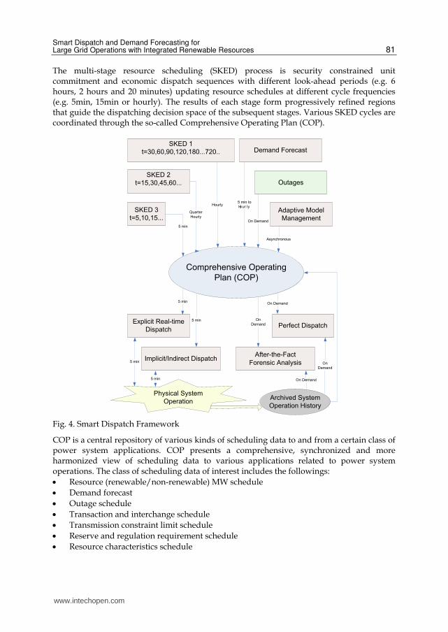
After-the-fact analysis for root-cause impacts and process re-engineering One major core functions of Smart Dispatch is called Generation Control Application (GCA) which aims at enhancing operators’ decision making process under changing system conditions (load, generation, interchanges, transmission constraints, etc.) in near real-time. GCA is composed of several distinct elements (Figure 4):

Multi-stage Resource Scheduling Process (SKED 1,2&3)

Comprehensive Operating Plan (COP)

Adaptive Model Management

www.intechopen.com


The multi-stage resource scheduling (SKED) process is security constrained unit commitment and economic dispatch sequences with different look-ahead periods (e.g. 6 hours, 2 hours and 20 minutes) updating resource schedules at different cycle frequencies (e.g. 5min, 15min or hourly). The results of each stage form progressively refined regions that guide the dispatching decision space of the subsequent stages. Various SKED cycles are coordinated through the so-called Comprehensive Operating Plan (COP).

Fig. 4. Smart Dispatch Framework

COP is a central repository of various kinds of scheduling data to and from a certain class of power system applications. COP presents a comprehensive, synchronized and more harmonized view of scheduling data to various applications related to power system operations. The class of scheduling data of interest includes the followings:

Resource (renewable/non-renewable) MW schedule

Demand forecast

Outage schedule

Transaction and interchange schedule

Transmission constraint limit schedule

Reserve and regulation requirement schedule

Resource characteristics schedule

www.intechopen.com


COP also contains comprehensive summary information. Summary information could be rollups from a raw data at a lower level (e.g. resource level) according to some pre-defined system structures. Adaptive Model Management as shown in Figure 4 consists of two parts: Advanced Constraint Modeling (ACM) and Adaptive Generator Modeling (AGM). ACM will use intelligent methods to preprocess transmission constraints based on historical and current network conditions, load forecasts, and other key parameters. It should also have ability to achieve smoother transmission constraint binding in time. AGM will provide other GCA components with information related to specific generator operational characteristics and performances. The resource “profiles” may contain parameters such as ramp rate, operating bands, predicted response per MW of requested change, high and low operating limits, etc. Another major core functions of Smart Dispatch is After-the Fact Analysis (AFA). AFA aims at providing a framework to conduct forensic analysis. AFA is a decision-support tool to: a. Identify root cause impacts and process re-engineering. b. Systematically analyze dispatch results based on comparison of actual dispatches with

idealized scenarios. c. Provide quantitative and qualitative measures for financial, physical or security impacts

on system dispatch due to system events and/or conditions. One special use case of AFA is the so-called “Perfect Dispatch” (PD). The idea of PD was originated by PJM (Gisin et al., 2010). PD calculates the hypothetical least bid production cost commitment and dispatch, achievable only if all system conditions were known and controllable. PD could then be used to establish an objective measure of RTO/TSO’s performance (mean of % savings, variance of % savings) in dispatching the system in the most efficient manner possible by evaluating the potential production cost saving derived from the PD solutions. Demand forecast is a very crucial input to GCA. The accuracy of it very much impacts market efficiency and system reliability. The following is devoted to discuss some recent advances in techniques of demand forecasting.

4. Demand forecast

Demand or load forecasting is very essential for reliable power system operations and market system operations. It determines the amount of system load against which real-time dispatch and day-ahead scheduling functions need to balance in different time horizon. Demand forecasting typically provides forecasts for three different time frames: 1. Short-Term (STLF): Next 60-120 minutes by 5-minute increments. 2. Mid-Term (MTLF): Next n days (n can be any value from 3-31), in intervals of one hour

or less (e.g., 60, 30, 20, 15 minute intervals). 3. Long-Term (LTLF): Next n years (n can be any value from 2-10), broken into one month

increments. The LTLF forecast is provided for three scenarios (pessimistic growth, expected growth, and optimistic growth).

Demand forecasting play an increasingly important role in the restructured electricity market and smart grid environment due to its impacts on market prices and market participants’ bidding behavior. In general, demand forecasting is a challenging subject in view of complicated features of load and effective data gathering. With Demand Response being one of the few near-term options for large-scale reduction of greenhouse gases, and fits strategically with the drive toward clean energy technology such as wind and solar, advanced

www.intechopen.com


demand forecasting should effectively take the demand response features/characteristics and the uncertainty of interimttent renewable generation into account. Many load forecasting techniques including extrapolations, autoregressive model, similar

day methods, fuzzy logic, Kalman filters and artificial neural networks. The rest of section will focus on the discussion of STLF which is a key input to near real-time generation

dispatch in market and system operations.

4.1 The uncertainty of demand forecast The uncertainty for demand forecast is one of the most critical factors influencing the

uncertainty of generation requirements for system balancing (DOE, 2010). It is important to note that wind generation has fairly strong positive correlation with electrical load in many

ways more than traditional dispatchable generation. As a result, it is viable to treat wind generation as a negative load and incorporate its uncertainty analysis as part of the

uncertainty of demand forecast assuming transmission congestion is not an issue. Hence, the concept of net demand has been employed in wind integration studies to assess the

impact of load and wind generation variability on the power system operations. Typically, the net demand has been defined as the following:

Net demand = Total electrical load – Renewable generation + Net interchange

One practical approach can be used for the uncertainty modeling of demand forecast is distribution fitting. Basically probability distributions are based on assumptions about a

specific standard form of random variables. Based on the standard distributions (e.g. normal) and selected set of its parameters (e.g. mean 航, standarddeviation購), they assign

probability to the event that the random variable x takes on a specific, discrete value, or falls within a specified range of continuous values. An example of the probability density

function PDF(x) (Meyer, 1970) of demand forecast is presented in Figure 5a. The cumulative distribution function CDF(x) can then be defined as:

系経繋岫捲岻 = 完鶏経繋岫嫌岻穴嫌掴貸著 (1)

A confidence interval (CI) is a particular kind of interval estimate of a population parameter

such that the random parameter is expected to lie within a specific level of confidence. A

confidence interval in general is used to indicate the reliability of an estimate and how likely

the interval to contain the parameter is determined by the confidence level (CL). The CL of

confidence interval [経健, 経ℎ] for demand forecast can be defined as:

系詣岫経健 ≤ 捲 ≤ 経ℎ岻 = 岶系経繋岫経ℎ岻 − 系経繋岫経健岻岼 × などど% (2)

Increasing the desired confidence level will widen the confidence interval being controlled

by parameters k1 and k2 as shown in Figure 5. It is obvious that the size of uncertainty

ranges depends on the look-ahead time. In general for longer look-ahead periods, the

uncertainty range becomes larger. Figure 6 illustrates the time-dependent nature of

confidence intervals – cone of uncertainty for demand forecast.

4.2 Artificial neural network with wavelet transform In the era of smart grid, the generation and load patterns, and more importantly, the way people use electricity, will be fundamentally changed. With intermittent renewable

www.intechopen.com


generation, advanced metering infrastructure, dynamic pricing, intelligent appliances and HVAC equipment, micro grids, and hybrid plug-in vehicles, etc., load forecasting with uncertain factors in the future will be quite different from today. Therefore, effective STLF are highly needed to consider the effects of smart grid.

Fig. 5. Probabilistic Uncertainty Model and Desired Confidence Interval for Demand Forecast

Fig. 6. Confidence Intervals for Demand Forecast

Based on frequency domain analysis, the 5-minute load data have multiple frequency

components. They can be illustrated via power spectrum magnitude. Figure 7 shows a

typical power spectrum of actual load of a regional transmission organization. Note that the

power density spectrum can be divided into multiple frequency ranges.

www.intechopen.com


0 0.125 0.25 0.375 0.5 0.625 0.75 0.875 1 10

20

30

40

50

60

70

80

90

100

110

Frequency

Power Spectrum Magnitude (dB)

Low

Freq.Medium

Frequency

High

Frequency

Fig. 7. A power spectrum density for 5-minute actual load

Neural networks have been widely used for load forecasting. They have been used for load forecasting in era of smart grid (Amjady et al., 2010; Zhang et al., 2010). In particular, Chen et al. have presented the method of similar day-based wavelet neural network approach (Chen, et al., 2010). The key idea there was to select “similar day load” as the input load, use wavelet decomposition to decompose the load into multiple components at different frequencies, apply separate neural networks to capture the features of the forecast load at individual frequencies, and then combine the results of the multiple neural networks to form the final forecast (see Figure 9). In general, these methods used general neural networks which adopted multilayer perception with the back-propagation training. There are many wavelet decomposition techniques. Some recent techniques applying to load forecasting are:

Daubechies 4 wavlet (Chen et al., 2010)

Multiple-level wavelet (Guan et al., 2010)

Dual-tree M-band wavelet (Guan et al., 2011) The Daubechies 4 (D4) wavelet is part of the family of orthogonal wavelets defining a discrete wavelet transform that decomposes a series into a high frequency series and a low frequency series. Multiple-level wavelet basically repeatedly applies D4 wavelet decomposition to the low frequency component of its previous decomposition as shown in Figure 8. Unlike D4 wavelet, Dual-tree M-band wavelet can selectively decompose a series into specified frequency ranges which could be key design parameters for more effective decomposition.

www.intechopen.com


L

Input Load

H NNH

NNLH

NNLLH

NNLLLH

NNLLLL

+

1-Level

2-Level

3-Level

LL LH

LLL LLH

LLLL LLLH

4-Level

1st

2nd

3rd

4th

5th

Relative Increment

Forecasts

Low Freq.

High Freqs.

Fig. 8. Multiple-level Wavelet Neural Network

In general, each (Neural Network) NN as shown in Figure 8 could be implemented as a feed-forward neural network being described by the following equation:

1 1( , , , , )t l t t t n tL f t L L L , (3)

where t is time of day, l is the time lead of the forecast, tL is the load component or relative

increment of the load component at time t and 1t represents a random load component.

The nonlinear function f is used to represent the nonlinear characteristics of a given neural

network.

4.3 Neural networks trained by hybrid kalman filters Since back-propagation algorithm is a first-order gradient-based learning algorithm, neural networks trained by such algorithm cannot produce the covariance matrix to construct dynamic confidence interval for the load forecasting. Replacing back-propagation learning, wavelet neural networks trained by hybrid Kalman filters are developed to forecast the load of next hour in five-minute steps with small estimated confidence intervals. If the NN input-output function was nearly linear, through linearization, NNs can be trained with the extended Kalman filter (EKFNN) by treating weight as state (Singhal & Wu, 1989). To speed up the computation, EKF was extended to the decoupled EKF by ignoring the interdependence of mutually exclusive groups of weights (Puskorius &Feldkamp, 1991). The numerical stability and accuracy of decoupled EKF was further improved by U-D factorization (Zhang & Luh, 2005). If the NN input-output function was highly nonlinear, EKFNN may not be good since mean and covariance were propagated via linearization of the underlying non-linear model. Unscented Kalman filter (Julier et al, 1995) was a potential method, and NNs trained by unscented Kalman filter (UKFNN) showed a superior performance. EKFNN was used to capture the feature of low frequency, and UKFNNs for those of higher frequency. Results are combined to form the final forecast. To capture the near linear relation between the input and output of the NN for the low component, a neural network trained by EKF is developed through treating the NN weight as the state and desired output as the observation. The input-output observations for the

www.intechopen.com


model can be represented by the set {u(t), z(t+1)}, where u(t) = {u1, …, unu}T is a nu×1 input vector, and z(t+1) = z(t+1|t) = {z1, …,znz}T is nz×1 a output vector. Correspondingly, ˆ ˆ( 1) ( 1 )z t z t t represents the estimation for measurement z(t+1). The formulation of

training NN through EKF (Zhang and Luh, 2005; Guan et al., 2010) can be described by state and measurement functions:

( 1)= ( )+ tw t w t , (4a)

( 1)= ( ), ( 1) + t+1z t h u t w t v , (4b)

where h(�) is the input-output function of the network, ε(t) and ν(t) are the process and measurement noises. The former is assumed to be white Gaussian noised with a zero mean and a covariance matrix Q(t), whereas the latter is assumed to have a student t-distribution with covariance matrix R(t). The weight vector w(t) has a dimension nw×1 and nw is determined by numbers of inputs, hidden neurons and outputs:

x h= n 1 n n 1w h zn n . (5)

Using the input vector u(t), weight vector w(t) and output vector ˆ( 1)z t , EKFNN are

derived. Key steps of derivation for EKF (Bar-Shalom et al. 2001) are summarized:

ˆ ( 1| ) ( | )w t t w t t , (6)

( 1| ) ( | ) ( )P t t P t t Q t , (7)

ˆ ˆ( 1| ) ( ), ( 1| )z t t h u t w t t , (8)

( 1) ( 1) ( 1| ) ( 1) ( 1)TS t H t P t t H t R t , (9)

( )ˆ ( 1| )

where ( 1) ( , ) u u tw w t t

H t h u w w , (10)

1( 1) ( 1| ) ( 1) ( 1)TK t P t t H t S t , (11)

ˆ ˆ ˆ( 1| 1) ( 1| ) ( 1) ( 1) ( 1| )w t t w t t K t z t z t t , (12)

( 1| 1) ( 1| ) ( 1) ( 1) ( 1| )P t t P t t K t H t P t t . (13)

where H(t+1) is the partial derivative of h(�) with respect to w(t) with dimension nz×nw, K(t+1) is the Kalman gain, P(t+1|t) is the prior weight covariance matrix and is updated to posterior weight covariance matrix P(t+1|t+1) based on the Bayesian formula, and S(t+1) is the measurement covariance matrix.

Let us denote ˆ ˆ1| 1|Lz t t z t t and 2ˆ ( 1) ( 1) 1 1T

L nyt S t I , where nyI is the

unit matrix, 1 1T is a vector with length of ny, 2ˆ ( 1)L t is the variance vector consists of

www.intechopen.com


the diagonal elements of S(t+1). ˆ 1|Lz t t and 2ˆ ( 1)L t representing the low frequency

component of prediction and variance, respectively, will be used for the final load

prediction and confidence interval estimation. Corresponding medium frequency

components of ˆ 1|Mz t t and 2ˆ ( 1)M t and high frequency components of ˆ 1|Hz t t

and 2ˆ ( 1)H t can be obtained via some UKFNN (Guan and et al., 2010).

4.4 Overall load forecasting and confidence interval estimation To quantify forecasting accuracy, the confidence interval was obtained by using the neural networks trained by hybrid Kalman filters. Within the wavelet neural network framework, the covariance matrices of Kalman filters for individual frequency components contained forecasting quality information of individual load components. When load components were combined to form the overall forecast, the corresponding covariance matrices would also be appropriately combined to provide accurate confidence intervals for the overall prediction (Guan et al., 2010).

The overall load prediction is the sum of low component prediction ˆLz , medium component

prediction ˆMz and high component prediction ˆ

Hz because these components are orthogonal

based on wavelet decomposition property:

ˆ ˆ ˆ ˆ( 1| ) ( 1| ) ( 1| ) ( 1| )L M Hz t t z t t z t t z t t , (14)

By the same token, the overall standard deviation ˆ( 1| )t t for STLF is the sum of standard

deviations for low and high components:

ˆ ˆ ˆ ˆ( 1| ) ( 1| ) ( 1| ) ( 1| )L M Ht t t t t t t t , (15)

Hence, the one sigma confidence interval for STLF can be constructed by:

ˆ ˆˆ ˆ( 1| ) ( 1| ), ( 1| ) ( 1| )z t t t t z t t t t . (16)

The overall scheme of training, forecasting and confidence interval estimation is depicted and summarized in Figure 9.

EKFNNH

UKFNNM

UKFNNL

+

High Freq.

Mediu Freq.

Low

Freq.

WD

Forecast

Time Indices

RI: Relative increment

WD: Wavelet Decomposition

EKFNN: Neural Networks Trained

by Extended Kalman Filter

UKFNN: Neural Networks Trained

by Unscented Kalman Filter

SD: Standard Deviation Derivation

RI

The Load of Last

Hour

SDH

SDM

SDL

+

Estimated

SD for CI

Fig. 9. Structure of a general wavelet neural networks trained by hybrid Kalman filters

www.intechopen.com


4.5 Composite demand forecasting To generate better forecasting results, a composite forecast is developed to mix multiple methods for STLF with CI estimation. The concept is based on the statistical model of ensemble forecasting to produce an optimal forecast by compositing forecasts from a number of different techniques. The method is depicted schematically in Figure 3.

Fig. 10. Ensemble forecasting

As illustrated in Figure 11, the method runs three sample models (Forecast 1, Forecast 2 and Forecast 3) in parallel. The weights of the combination are theoretically derived based on the “interactive multiple model” approach (Bar-Shalom et al, 2001). For methods which are based on Kalman filters and have dynamic covariance matrices on the forecast load, these dynamic covariance matrices are used for the combination. Otherwise, static covariance matrices derived from historic forecasting accuracy are used instead.

z(t+1|t) S(t+1)

3(t)

µ(t)

Forecast 3

z2(t+1|t)

SD2(t+1)

CLFCC MPC

Forecast 1

1(t)

z(t)

z1(t+1|t)

S1(t+1)

z(t)

Forecast 2

z(t)

2(t)z3(t+1|t)

SD3(t+1)

CLFCC: Composite load forecasting and covariance combination

MPC: Mixing probability calculation

Fig. 11. Structure of composite forecasting with confidence interval estimation

www.intechopen.com


The relative increment (RI) in load is used to help capture the load features in the method since it removes a first-order trend and anchor the prediction by the latest load (Shamsollahi et al., 2001). After normalization, the RI in load of last time period z(t) is denoted as the input to the NN, where time t is the time index. The mixing weight µ(t) can

be calculated through the likelihood functions j(t), with superscript j=1, 2, 3 representing Forecasts 1, 2 &3 respectively:

( ) ( ); | 1 , ( )]jj jt N z t z t t S t , (17)

3

1

( ) ( ) ( )j jj j jj

t t c t c

,

3

1

( 1) 1,2,3j ij ii

where c p t j

, (18)

where p is the transition probability to be configured manually. S1, S2 and S3 are sample covariance matrices from Forecasts 1, 2 &3 derived from historic forecasting accuracy. Without loss of generality, we assume that dynamic covariance matrices S2D for Forecast 2 and S3D for Forecast 3 are available. To make a stable combination, the dynamic innovation matrices S2D from Forecast 2 and S3D from Forecast 3 are not used to calculate

likelihood functions 2 and 3 since S2D and S3D may largely affects the mixing weight. Then predictions from individual models can be combined to form the forecast:

3

1

( 1| ) ( 1| )jj

j

z t t t z t t

. (19)

The output z(t+1|t) from NNs has to be transformed back due to the RI transformation on the load input. Similar to the prediction combination, the static covariance matrix S1 derived from historic forecasting accuracy and dynamic covariance matrices S2D and S3D will also be combined. Here, S1 S2D and S3D are the covariance matrices for NN outputs (estimated RI in load). Since RI is a nonlinear transformation, the covariance matrix has to be transformed. If S1 S2D and S3D can be obtained directly from individual models, they can be combined first:

1 1 2 2 3 3( 1) ( 1) ( 1) ( 1)D DS t t S t t S t t S t (20)

Then, S(t+1) will be used to further derive CIs with respect to RI transformation (Guan et al., 2010). Demand forecast and its corresponding confidence intervals are crucial inputs to the Generation Control Application which robustly dispatch the power system using a series of coordinated scheduling functions.

5. Generation control application

Generation Control Application (GCA) is an application designed to provide dispatchers in large power grid control centers with the capability to manage changes in load, generation,

www.intechopen.com


interchange and transmission security constraints simultaneously on a intra-day and near real-time operational basis. GCA uses least-cost security-constrained economic scheduling and dispatch algorithms with resource commitment capability to perform analysis of the desired generation dispatch. With the latest State Estimator (SE) solution as the starting point and transmission constraint data from the Energy Management System (EMS), GCA Optimization Engines (aka Scheduler or SKED) will look ahead at different time frames to forecast system conditions and alter generation patterns within those timeframes. This rest of this section will focus on the functionality of SKED engines and its coordination

with COP.

5.1 SKED optimization engine SKED is a Mixed Integer Programming (MIP) / Linear Programming (LP) based optimization

application which includes both unit commitment and unit dispatch functions. SKED can be

easily configured to perform scheduling processes with different heart beats and different

look-ahead time. A typical configuration for GCA includes three SKED sequences:

SKED1 provides the system operator with intra-day incremental resource (including

generators and demand side responses) commitment/de-commitment schedules based

on Day-ahead unit commitment decision to manage forecasted upcoming peak and

valley demands and interchange schedules while satisfying transmission security

constraints and reserve capacity requirements. SKED1 is a MIP based application. It is

typically configured to execute for a look-ahead window of 6-8 hours with viable

interval durations, e.g., 15-minute intervals for the 1st hour and hourly intervals for the

rest of study period.

SKED2 will look 1-2 hour ahead with 15-minute intervals. SKED2 will fine-tune the

commitment status of qualified fast start resources and produce dispatch contours.

SKED2 also provides resource ramping envelopes for SKED3 to follow (Figure 12).

SKED3 is a dispatch tool which calculates the financially binding base points of the next

five-minute dispatch interval and advisory base-points of the next several intervals for

each resource (5 min, 10 min, 15 min, etc). SKED3 can also calculate ex-ante real-time

LMPs for the financial binding interval and advisory price signals for the rest of study

intervals. SKED3 is a multi-interval co-optimization LP problem. Therefore, it could

pre-ramp a resource for the need of load following and real-time transmission

congestion management.

Traditionally, due to the uncertainty in the demand and the lack of compliance from

generators to follow instructions, RTOs have to evaluate several dispatch solutions for

different demand scenarios (low (L), medium (M) and high (H)). Figure 4 depicts such practice

for real-time dispatch. Except for the initial conditions (e.g. MW from State Estimator (SE)), the

solutions are independent. The operators have to choose to approve one of the three load

scenarios based on their human judgments on which scenario is more likely to occur.

The conventional way of dealing with the demand uncertainty is stochastic optimization

(Wu et al., 2007; Verbic and Cañizares, 2006; Ruiz et al., 2009). The data requirements of

stochastic optimization, makes it more appropriate to solve longer term problems, e.g.

expansion and operational planning, including day-ahead security constrained unit

commitment process. However, the simplicity and flexibility of the solution proposed in this

chapter makes it more practical for real-time dispatch.

www.intechopen.com


Fig. 12. SKED 2 and SKED 3 Coordination

A. Single interval dispatch model

The traditional single interval dispatch model is formulated as a Linear Programming (LP) problem:

*i ii

Minimize

c Pg

min max

,

max max,

( ) * ( ) *

*

ii

i i i

SE i i iSE SE i t

k Fk i i ki

subject to

Pg Dm

Pg Pg Pg

time time RRDn Pg Pg time time RRUp

F Dfax Pg F

(21)

where

ic Offer price for resource i

iPg Dispatch level for resource i

Dm Demand forecast for target time min max,i iPg Pg Min and max dispatch level for resource i

maxkF Line/flowgate k transmission limit

,Fk iDfax Sensitivity of line/flowgate k to injection i (demand distributed slack)

time Target time

SEtime State Estimator time stamp

iRRDn Maximum ramp rate down for resource i

iRRUp Maximum ram rate up for resource i

www.intechopen.com


Fig. 13. Three independent dispatch solutions

B. Dynamic dispatch model

Adding the time dimension into the single interval dispatch problem above described, the basic

multi-interval dispatch (dynamic dispatch) model is formulated as an extended LP problem

(sub-index t is added to describe interval t related parameters and variables, as appropriate):

, , 1* * ( ) /60i t i t t tt i

Minimize

c Pg Time Time

,

min max, , ,

1 , , , 1 1 ,

max max, , , ,

( ) * ( ) *

*

i t ti

i t i t i t

t t i t i t i t t t i t

k t Fk i i t k ti

subject to

Pg Dm

Pg Pg Pg

time time RRDn Pg Pg time time RRUp

F Dfax Pg F

(22)

{ 1,... }for t t tn

Figure 13. illustrates the dynamic dispatch model with multiple scenario runs.

C. Robust dispatch model

A more robust solution that co-ordinates the three demand scenarios, guaranteeing the

"reach-ability" of confidence interval of demand forecast from the medium demand dispatch

is proposed.

www.intechopen.com


The solution would provide a single robust dispatch, guaranteeing that the dispatch levels for the low and high demand scenarios can be reached from the dispatch corresponding to the medium (expected) demand scenario within consecutive intervals in the study horizon, e.g. avoiding extreme measures like demand curtailment if the high demand scenario materializes and it is too late to catch up. The robust solution proposed is depicted in Figure 14. The cost of Robust Dispatch will be higher than ordinary dispatch using medium load level. It can be justified as a type of ancillary services for load following. A further refinement to the proposed solution is to limit the cost of the “robustness” and specify a merit order of the intervals in which robustness is more valuable.

Fig. 14. Robust dispatch solution

The following LP problem co-ordinates the three demand scenarios into one “robust” solution. The objective function and constraints corresponding to the medium demand scenario are the same as those of an independent dynamic dispatch (M only); for the high and low demand scenarios, however, while the objective function terms are the same as those of independent dynamic dispatches (H only and L only), the maximum ramp rate constraints for each resource do not link dispatch levels of consecutive intervals for the same scenario (H→H, L→L); instead, for a given interval t such constraints link the H and L dispatch levels with the dispatch level corresponding to the M scenario in the preceding interval t-1 (M→H and M→L); guaranteeing the "reach-ability" of the low and high demand scenarios dispatches from the medium demand dispatch level in successive intervals (upper and lower case h, m and l are used as extensions to describe high, medium and low demand scenarios parameters and variables).

www.intechopen.com


, , 1

, , 1

, , 1

* * ( ) /60

* * ( ) /60

* * ( ) /60

i t i t t tt i

i t i t t tt i

i t i t t tt i

Minimize

c Pgm time time

c Pgh time time

c Pgl time time

subject to

,

min max, , ,

1 , , , 1 1 ,

max max, , , , ,

( ) * ( ) *

*

i t ti

i t i t i t


k t Fk i t i t k ti

Pgm Dm

Pg Pgm Pg

time time RRDn Pgm Pgm time time RRUp

F Dfax Pgm F

,

min max, , ,

1 , , , 1 1 ,

max max, , , , ,

( ) * ( ) *

*

i t ti

i t i t i t


k t Fk i t i t k ti

Pgh Dh

Pg Pgh Pg

time time RRDn Pgh Pgm time time RRUp

F Dfax Pgh F

(23)

,

min max, , ,

1 , , , 1 1 ,

max max, , , , ,

( ) * ( ) *

*

i t ti

i t i t i t


k t Fk i t i t k ti

Pgl Dl

Pg Pgl Pg

time time RRDn Pgl Pgm time time RRUp

F Dfax Pgl F

{ 1,... }for t t tn

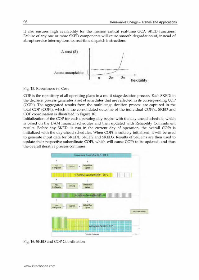
It is important to note that there is certainly a tradeoff between cost and robustness for any given robust dispatch solution using the methodology proposed above. Figure 15 illustrates the conceptual idea of relationship between cost and flexibility which is proportional to robustness. The value of the “∆cost acceptable” will be very much dependent on the amount of risk one is willing to take for reliability purposes when dispatching the system.

5.2 SKED and COP coordination GCA is built upon a modular and flexible system architecture. Although different SKED processes are correlated, they do not replay on each other. The orchestration between SKEDi is managed by COP. This design enables low-risk, cost-effective business process evolution.

www.intechopen.com


It also ensures high availability for the mission critical real-time GCA SKED functions. Failure of any one or more SKED components will cause smooth degradation of, instead of abrupt service interruptions to, real-time dispatch instructions.

Fig. 15. Robustness vs. Cost

COP is the repository of all operating plans in a multi-stage decision process. Each SKEDi in the decision process generates a set of schedules that are reflected in its corresponding COP (COPi). The aggregated results from the multi-stage decision process are captured in the total COP (COPt), which is the consolidated outcome of the individual COPi’s. SKED and COP coordination is illustrated in Figure 16. Initialization of the COP for each operating day begins with the day-ahead schedule, which is based on the DAM financial schedules and then updated with Reliability Commitment results. Before any SKEDi is run in the current day of operation, the overall COPt is initialized with the day-ahead schedules. When COPt is suitably initialized, it will be used to generate input data for SKED1, SKED2 and SKED3. Results of SKEDi’s are then used to update their respective subordinate COPi, which will cause COPt to be updated, and thus the overall iterative process continues.

Fig. 16. SKED and COP Coordination

www.intechopen.com


GCA aims at enhancing operators’ forward-looking view under changing system conditions (generation capacity, ramp capability, transmission constraints, etc.) and providing operators with a “radar-type” of recommendation of actions such as startup or shutdown of fast-start resources in near real-time. As shown in Figure 17 – COP review display, various startup and shutdown recommendations are approaching the “now” timeline like an 1-dimensional radar sorted by likelihood ranking from top to bottom. The COP review display also shows actual system total generation and comparing against demand forecast and system ramp constrained capacity. This provides situation awareness of any potential abrupt ramping events or potential system imbalance and alerts operators in advance if any actions need to be taken.

Fig. 17. Forward-looking view presented by COP Overview

6. Conclusion

Significant capacity of renewable generation resources operating online at any given time is of great concern to grid security due to the intermittent nature of many of the resources. On one hand, the potential volatility of the intermittent generation output could cause great stress on the system’s generation planning and ramp management. On the other hand, these intermittent resources could be operating at locations that contribute to transmission line congestion and become very challenging problems for a lot of the RTOs. This chapter addresses the challenges of renewable integration from a generation dispatch perspective. The framework of Smart Dispatch is proposed in which the

www.intechopen.com


applications of demand forecasting and robust dispatch are discussed in detail. A new dispatch system called Generation Control Application (GCA) is described to address the challenges posed by renewable energy integration. GCA aims at enhancing operators’ forward-looking view under changing system conditions such as wind speed or other weather conditions. GCA provides operators with situation awareness of any potential abrupt ramping events or potential system imbalance and alerts operators in advance if any actions need to be taken. With dynamic and robust dispatch algorithm and flexible system configuration, the system provides adequate system ramping capability to cope with uncertain intermittent resources while maintaining system reliability in large grid operations. Smart Dispatch is deemed critical for the success of efficient power system operations in the near future.

7. Acknowledgment

The views expressed in this chapter are solely those of the author, and do not necessarily represent those of Alstom Grid.

8. References

Amjady, N.; Keynia, F. &Zareipour, H. (2010). Short-Term Load Forecast of Microgrids by a New Bilevel Prediction Strategy, Smart Grid, IEEE Transactions on, vol.1, no.3, pp.286-294, Dec. 2010.

Bar-Shalom, Y.; Li, X. R. & Kirubarajan, T. (2001). Estimation with Applications to Tracking and Navigation: Algorithms and Software for Information Extraction, J. Wiley and Sons, pp.200-209 and pp.385-386.

Chen, Y.; Luh, P. B.; Guan, C.; Zhao, Y. G.; Michel, L. D.; Coolbeth, M. A.; Friedland, P. B. & Rourke, S. J. (2010). Short-term Load Forecasting: Similar Day-based Wavelet Neural Networks, IEEE Transaction on Power Systems, 25(1):322-330.

Cheung, K. W.; Wang, X.; Chiu, B. -C.; Xiao, Y. & Rios-Zalapa, R. (2010). Generation Dispatch in a Smart Grid Environment, Proceedings of 2010 IEEE/PES Innovative Smart Grid Technologies Conference (ISGT 2010).

Cheung, K. W.; Wang, X. & Sun, D. (2009). Smart Dispatch of Generation Resources for Restructured Power Systems, Proceedings of the 8th IET International Conference on Advances in Power System Control, Operation and Management.

Chow, J. H.; deMello, R. & Cheung, K. W. (2005). Electricity Market Design: An Integrated Approach to Reliability Assurance. (Invited paper), IEEE Proceeding (Special Issue on Power Technology & Policy: Forty Years after the 1965 Blackout), vol. 93, pp.1956-1969, Nov. 2005.

Chuang, A. S. & Schwaegerl, C. (2009). Ancillary services for renewable integration, Integration of Wide-Scale Renewable Resources into the Power Delivery System, 2009 CIGRE/IEEE PES Joint Symposium.

DOE’s Report (2010). Incorporating Wind Generation and Load Forecast Uncertainties into Power Grid Operations, PNNL-19189.

Gisin, B.; Qun Gu; Mitsche, J.V.; Tam, S. & Chen, H. (2010). “Perfect Dispatch” – as the Measure of PJM Real Time Grid Operational Performance, Proceedings of the IEEE PES 2010 General Meeting.

www.intechopen.com


Guan, C.; Luh, P. B.; Cao, W.; Zhao, Y.; Michel, L. D. & Cheung, K. W. (2011). Dual-tree M-band Wavelet Transform and Composite Very Short-term Load Forecasting, Proceedings of the IEEE PES 2011 General Meeting.

Guan, C.; Luh, P. B.; Coolbeth, M. A.; Zhao, Y.; Michel, L. D.; Chen, Y.; Manville, C. J.; Friedland, P. B. & Rourke, S. J. (2009). Very Short-term Load Forecasting: Multilevel Wavelet Neural Networks with Data Pre-filtering, Proceedings of the IEEE PES 2009 General Meeting.

Guan, C.; Luh, P.B.; Michel, L.D.; Coolbeth, M.A. & Friedland, P.B. (2010). Hybrid Kalman algorithms for very short-term load forecasting and confidence interval estimation, Power and Energy Society General Meeting, 2010 IEEE , vol., no., pp.1-8, 25-29 July 2010.

Julier, S. J.; Uhlman, J. K. & Durrant-Whyte, H. F. (1995). A New Approach for Filtering Nonlinear Systems, In Proc. American Control Conf, Seattle, WA, 1628-1632.

Ma, X.-W.; Sun, D. & Cheung, K. W. (1999). Energy and Reserve Dispatch in a Multi-Zone Electricity Market, IEEE Transaction of Power Systems, vol. 14, pp.913-919, Aug. 1999.

Meyer, P. L. (1970). Introductory Probability and Statistical Applications, Addison-Wesley Publishing Company, Inc., 1970.

Puskrius, G. V. & Feldkamp, L. A. (1991). Decoupled Extended Kalman Filter Training of Feedforward Layered Networks, Proceedings of IEEE International Joint Conference on Neural Networks, 771-777.

Rios-Zalapa, R.; Wang, X.; Wan, J. & Cheung, K. W. (2010). Robust Dispatch to Manage Uncertainty in Real Time Electricity Markets, Proceedings of 2010 IEEE/PES Innovative Smart Grid Technologies Conference (ISGT 2010).

Ruiz, P. A.; Philbrick, C. R.; Zak, E.; Cheung, K. W. & Sauer, P. W. (2009). Uncertainty Management in the Unit Commitment Problem, IEEE Transactions on Power Systems, Vol. 24, No. 2, May 2009, pp. 642-651.

Schweppe, F. C.; Caramanis, M. C.; Tabors, R. D. & Robn, R. E. (1998). Spot Pricing of Electricity, Kluwer Academic Publishers, 1998.

Shamsollahi, P.; Cheung, K. W.; Chen, Q. & Germain, E. H. (2001). A Neural Network Based Very Short term Load Forecaster for the Interim ISO New England Electricity Market System, Proceedings of the 22nd International Conference on Power Industry Computer Applications, pp.217-222 (2001).

Singhal, S. & Wu, L. (1989). Training feed-forward networks with the extended Kalman filter, Proceedings of IEEE International Conference on Acoustics Speech and Signal Processing, 1187–1190.

Verbic, G. & Cañizares, C. A. (2006). Probabilistic Optimal Power Flow in Electricity Markets Based on a Two-Point Estimate Method, IEEE Transactions on Power Systems, Vol. 21, No. 4, November 2006, pp. 1883-1893.

Wood, A. J. & Wollenberg, B. F. (1996). Power Generation, Operation, and Control, second edition, John Wiley & Sons, New York, 1996.

Wu, L.; Shahidehpour, M.; Li, T. (2007). Stochastic Security-Constrained Unit Commitment, IEEE Transactions on Power Systems, Volume: 22, No. 2, May 2007.

Zhang, H.–T.; Xu, F.-Y. & Zhou, L. (2010). Artificial neural network for load forecasting in smart grid, Machine Learning and Cybernetics (ICMLC), 2010 International Conference on, vol.6, no., pp.3200-3205, July 11-14, 2010.

www.intechopen.com


Zhang, L. & Luh, P. B. (2005). Neural Network-based Market Clearing Price Prediction and Confidence Interval Estimation with an Improved Extended Kalman Filter Method, IEEE Transactions on Power Systems, Vol. 20, No. 1, February, 2005, pp. 59-66.

www.intechopen.com

Renewable Energy - Trends and ApplicationsEdited by Dr. Majid Nayeripour

ISBN 978-953-307-939-4Hard cover, 250 pagesPublisher InTechPublished online 09, November, 2011Published in print edition November, 2011

InTech EuropeUniversity Campus STeP Ri Slavka Krautzeka 83/A 51000 Rijeka, Croatia Phone: +385 (51) 770 447 Fax: +385 (51) 686 166www.intechopen.com

InTech ChinaUnit 405, Office Block, Hotel Equatorial Shanghai No.65, Yan An Road (West), Shanghai, 200040, China

Phone: +86-21-62489820 Fax: +86-21-62489821

Increase in electricity demand and environmental issues resulted in fast development of energy productionfrom renewable resources. In the long term, application of RES can guarantee the ecologically sustainableenergy supply. This book indicates recent trends and developments of renewable energy resources thatorganized in 11 chapters. It can be a source of information and basis for discussion for readers with differentbackgrounds.

How to referenceIn order to correctly reference this scholarly work, feel free to copy and paste the following:

Kwok W. Cheung (2011). Smart Dispatch and Demand Forecasting for Large Grid Operations with IntegratedRenewable Resources, Renewable Energy - Trends and Applications, Dr. Majid Nayeripour (Ed.), ISBN: 978-953-307-939-4, InTech, Available from: http://www.intechopen.com/books/renewable-energy-trends-and-applications/smart-dispatch-and-demand-forecasting-for-large-grid-operations-with-integrated-renewable-resources

© 2011 The Author(s). Licensee IntechOpen. This is an open access articledistributed under the terms of the Creative Commons Attribution 3.0License, which permits unrestricted use, distribution, and reproduction inany medium, provided the original work is properly cited.

http://creativecommons.org/licenses/by/3.0

Smart Dispatch and Demand Forecasting for Large Grid Operations

Documents

Transcript of Smart Dispatch and Demand Forecasting for Large Grid Operations