SLURRY TRANSPORT USING CENTRIFUGAL PUMPS

Third Edition

SLURRY TRANSPORT USING CENTRIFUGAL PUMPS

Third Edition

K. C. WILSON Queen's University

Kingston, Ontario, Canada

G. R. ADDIE GIW Industries Inc.

Grovetown, Georgia, USA

A. SELLGREN Lulea University of Technology

Lulea, Sweden

R. CLIFT University of Surrey

Guildford, Surrey, UK

Springer

Library of Congress Cataloging-in-Publication Data

A C.I.P. Catalogue record for this book is available from the Library of Congress.

ISBN-10: 0-387-23262-1 ISBN-10: 0-387-23263-X (e-book) ISBN-13: 9780387232621 ISBN-13: 9780387232638

Printed on acid-free paper.

© 2006 Springer Science-I-Business Media, Inc. All rights reserved. This work may not be translated or copied in whole or in part without the written permission of the publisher (Springer Science+Business Media, Inc., 233 Spring Street, New York, NY 10013, USA), except for brief excerpts in connection with reviews or scholarly analysis. Use in connection with any form of information storage and retrieval, electronic adaptation, computer software, or by similar or dissimilar methodology now known or hereafter developed is forbidden. The use in this publication of trade names, trademarks, service marks and similar terms, even if they are not identified as such, is not to be taken as an expression of opinion as to whether or not they are subject to proprietary rights.

Printed in the United States of America.

9 8 7 6 5 4 3 2 1 SPIN 11327295

springeronline.com

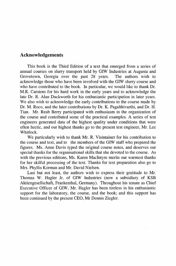
Acknowledgements

This book is the Third Edition of a text that emerged from a series of annual courses on slurry transport held by GIW Industries at Augusta and Grovetown, Georgia over the past 28 years. The authors wish to acknowledge those who have been involved with the GIW slurry course and who have contributed to the book. In particular, we would like to thank Dr. M.R. Carstens for his hard work in the early years and to acknowledge the late Dr. R. Alan Duckworth for his enthusiastic participation in later years. We also wish to acknowledge the early contributions to the course made by Dr. M. Roco, and the later contributions by Dr. K. Pagalthivarthi, and Dr. H. Tian. Mr. Reab Berry participated with enthusiasm in the organization of the course and contributed some of the practical examples. A series of test engineers generated data of the highest quality under conditions that were often hectic, and our highest thanks go to the present test engineer, Mr. Lee Whitlock.

We particularly wish to thank Mr. R. Visintainer for his contribution to the course and text, and to the members of the GIW staff who prepared the figures. Ms. Anne Davis typed the original course notes, and deserves our special thanks for the organisational skills that she devoted to the course. As with the previous editions, Ms. Karen Maclntyre merits our warmest thanks for her skilful processing of the text. Thanks for text preparation also go to Mrs. Phyllis Korman and Mr. David Nielsen.

Last but not least, the authors wish to express their gratitude to Mr. Thomas W. Hagler Jr. of GIW Industries (now a subsidiary of KSB Aktiengesellschaft, Frankenthal, Germany). Throughout his tenure as Chief Executive Officer of GIW, Mr. Hagler has been tireless in his enthusiastic support for the laboratory, the course, and the book; and this support has been continued by the present CEO, Mr Dennis Ziegler.

Contents

Chapter 1 - Introduction 1.1 Applications of Slurry Transport 1 1.2 Topics Covered in this Book 4 1.3 List of Symbols 9

Chapter 2 - Review of Fluid and Particle Mechanics 2.1 Introduction 15 2.2 Basic Relations for Flow of Simple Fluids 18 2.3 Friction in Laminar and Turbulent Flow of Simple Fluids 23 2.4 Basic Relations for Slurry Flow 35 2.5 Settling of Solids in Liquids 39

Chapter 3 - Flow of Non-Settling Slurries 3.1 Introduction 51 3.2 Rheometry and Rheological Models 54 3.3 Turbulent Flow of Non-Newtonians 60 3.4 Scale-up of Laminar Flow 66 3.5 Scale-up of Turbulent Flow 67 3.6 Effects of Solids Concentration 72 3.7 Transition from Laminar to Turbulent Flow 73 3.8 Case Study 76

Chapter 4 - Principles of Particulate Slurry Flow 4.1 Introduction 83 4.2 Homogeneous and Pseudo-Homogeneous Flow 84 4.3 Flow of Settling Slurries 86 4.4 Physical Mechanisms Influencing Type of Flow 91 4.5 Stationary Deposits of Solids 94 4.6 Heterogeneous Flow 95 4.7 Specific Energy Consumption 98

Chapter 5 - Motion and Deposition of Settling Sohds 5.1 Introduction 102 5.2 Resisting and Driving Forces 103

Vlll

5.3 Velocity at the Limit of Stationary Deposition 108 5.4 Effect of Solids Concentration on Deposit Velocity 113 5.5 Fully Stratified Coarse-Particle Transport 113 5.6 Case Studies 117

Chapter 6 - Heterogeneous Slurry Flow in Horizontal Pipes 6.1 Introduction 123 6.2 Concepts of Near-Wall Hydrodynamic Lift 125 6.3 Stratification Ratio and Scale-up 128 6.4 Effect of Particle Size Distribution 136 6.5 Simplified Approach for Estimating Solids Effect 141 6.6 Effect of Large Pipe Diameter 142 6.7 Effect of High Concentration of Solids 143 6.8 Case Studies 145

Chapter 7 - Complex Slurries 7.1 Introduction 152 7.2 Broad-graded Slurries with Newtonian Carrier Fluids 153 7.3 The 'Stabflo' Debate 157 7.4 Particle Settling in non-Newtonian Fluids 160 7.5 Particle Settling in Laminar non-Newtonian Pipeline Flow 162 7.6 Turbulent Flow of Slurries with non-Newtonian Carrier Fluids 163 7.7 Example Problems and Case Study 165

Chapter 8 ~ Vertical and Indined Slurry Flow 8.1 Introduction 172 8.2 Analysis of Vertical Flow 173 8.3 Applications of Vertical Flow 177 8.4 Effect of Pipe Inclination on Deposition Limit 179 8.5 Effect of Pipe Inclination on Friction Loss 181 8.6 Worked Examples and Case Study 184

Chapter 9 - Centrifugal Pumps 9.1 Introduction: Basic Concepts and Affinity Laws 190 9.2 Hydraulic Design and Specific Speed 196 9.3 Cavitation and Net Positive Suction Head 208 9.4 Mechanical Design 213 9.5 Performance Testing 217 9.6 Case Studies 222

IX

Chapter 10 - Effect of Solids on Pump Performance 10.1 Introduction and Previous Correlations 227 10.2 Effect of Pump Size 234 10.3 Effect of Solids Concentration 235 10.4 Effect of Particle Properties 237 10.5 Non-settling Slurries 238 10.6 Suction Performance 241 10.7 Generalised Solids-Effect Diagram for Settling Slurries 241

Chapter 11 - Wear and Attrition 11.1 Introduction 249 11.2 Wear-Resistant Materials 253 11.3 Combined Erosion and Corrosion 256 11.4 Experimental Testing Methods 257 11.5 Numerical Modelling of Flow and Wear 263 11.6 Pump and Wear Variables 267 11.7 Variation of Wear with Design Geometry 269 11.8 Variation of Component Wear with Different Duties 272 11.9 Practical Considerations and Field Experience 273 11.10 Particle Attrition 279

Chapter 12 - Components of Slurry Systems 12.1 Introduction 286 12.2 Pump Suction Piping Considerations 287 12.3 Pump Drive Trains 294 12.4 Pump Layout and Spacing 298 12.5 Flow Control and Valving 301 12.6 Instrumentation 304

Chapter 13 - System Design and Operabihty 13.1 Introduction 312 13.2 Homogeneous Slurries 313 13.3 Effect of Solids Concentration in Settling Slurries 318 13.4 Effect of Particle Size 323 13.5 Case Study 329

Chapter 14 - Pump Selection and Cost Considerations 14.1 General Concepts of Pump Selection 338 14.2 Wear Considerations 341

14.3 Economic Considerations 342 14.4 Downtime Costs 347 14.5 Effect of System Size 349 14.6 Selection Procedure 350

Chapter 15 - Practical Experience with Slurry Systems 15.1 Introduction 353 15.2 Pumps in Series 354 15.3 Pumps in Parallel 359 15.4 Suction Problems 360 15.5 Pumping Frothy Mixtures 361 15.6 Flow Instability 364 15.7 Operation with a Stationary Bed 367 15.8 Transient Conditions 369

Chapter 16 - Environmental Aspects of Slurry Systems 16.1 Introduction 377 16.2 The Benefits of Integrated Processing 378 16.3 Energy Consumption and Associated Emissions 381 16.4 A Cautionary Tale - Velenje and its Lakes 385

Appendix - Worked Examples and Case Studies in U.S. Customary Units 390

Index 427

Chapter 1

INTRODUCTION

1,1 Applications of Slurry Transport

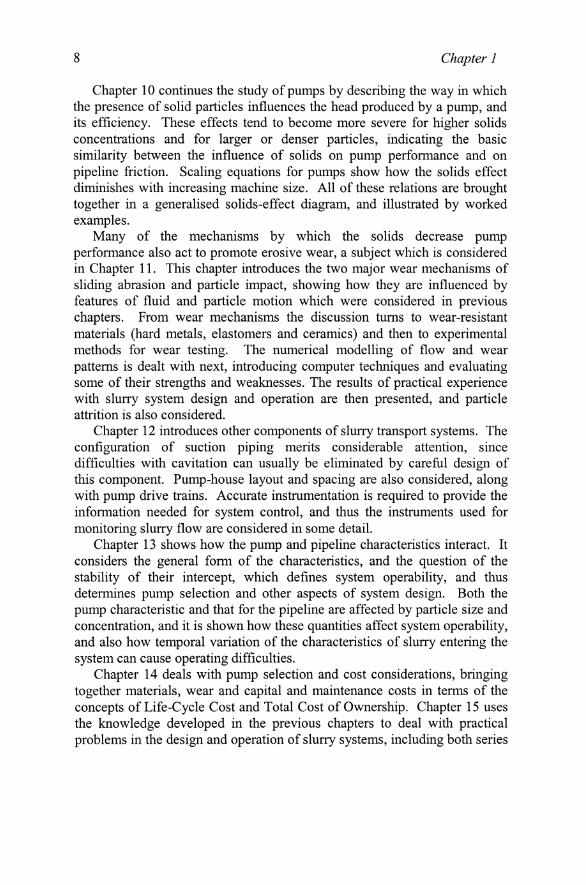
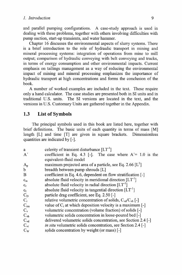
Vast tonnages are pumped every year in the form of solid-liquid mixtures, known as slurries. The application which involves the largest quantities is the dredging industry, continually maintaining navigation in harbours and rivers, altering coastlines and winning material for landfill and construction purposes. As a single dredge may be required to maintain a throughput of 7000 tonnes of slurry per hour or more, very large centrifugal pumps are used. Figures 1-1 and 1-2 show, respectively, an exterior view of this type of pump, and a view of a large dredge-pump impeller (Addie & Helmley, 1989).

The manufacture of fertiliser is another process involving massive slurry-transport operations. Li Florida, phosphate matrix is recovered by huge draglines in open-pit mining operations. It is then slurried, and pumped to the wash plants through pipelines with a typical length of about 10 kilometres. Each year some 34 million tonnes of matrix are transported in this manner. This industry employs centrifugal pumps that are generally smaller than those used in large dredges, but impeller diameters up to 1.4 m are common, and drive capacity is often in excess of 1000 kW. The transport distance is typically longer than for dredging applications, and

Chapter 1

Figure LI. Testing a dredge pump at the GIW Hydraulic Laboratory

Figure 1.2. Impeller for large dredge pump

1. Introduction 3

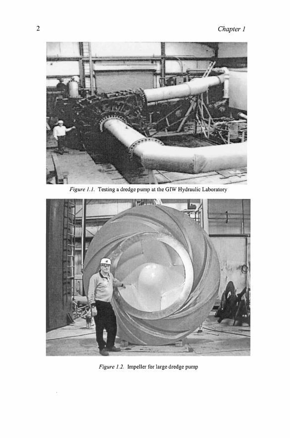
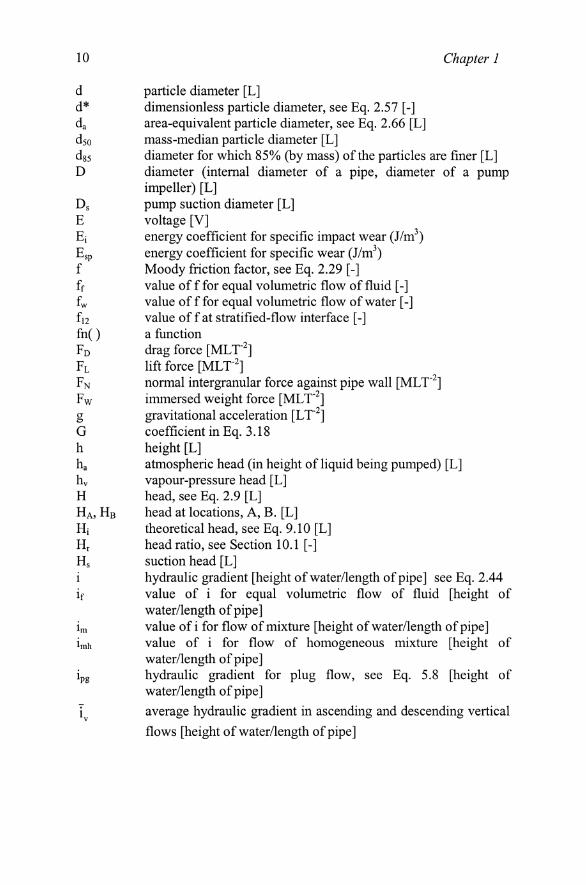
hence a series of pumping stations is often used. Figure 1-3 shows a booster-pump installation in a phosphate pipeline.

Many other types of open-pit mining use slurry transport, and the number of such applications is increasing as it becomes clear that, for many short-haul and medium-haul applications, slurry transport is more cost-effective than transport by truck or conveyor belt. Partially-processed material from mining and metallurgical operations and other industries is often already in slurry form, facilitating pipe transport. Much of this is carried out using relatively small lines. For example newly-mixed concrete is a slurry and is sometimes piped from the mixing plant to other parts of a construction site.

Figure 1.3. Booster pump in a phosphate-matrix pipeUne

As this slurry has a high resistance to flow, and as considerable static lifts are also common in construction, the pumps employed are usually of the positive-displacement type. Such pumps are also used in other high-head applications; and the best-known of these is the Black Mesa pipeline which transports a partially-processed coal slurry from the mine to a electrical generating station more than 400 km distant. This line, which involves heads at each pumping section of 75 atmospheres or more, began operation in 1970. Since that time many similar, but larger, coal pipelines have been proposed, but none has yet been built.

Recent decades have seen a great increase in the transport of waste materials, in slurry form, to suitable deposit sites. The concept is an old one and the earliest known use was by Hercules, who removed a decade's accumulation of animal droppings from King Augeas' stables by diverting two rivers to form an open-channel slurry transport system. Waste-disposal

4 Chapter 1

problems are even more severe at present, and maintenance of the environment requires that wastes be conveyed to dedicated and monitored disposal sites, either underground or on the surface. This requirement can often be satisfied by backfilling mines (either deep or open-pit), and slurry transport is the favoured placing method. Such backfilling operations are usually characterised by significant tonnages with short to medium hauls, and hence centrifugal pumps are the natural choice for these applications.

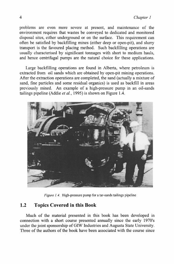
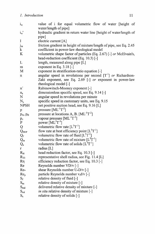
Large backfilling operations are found in Alberta, where petroleum is extracted from oil sands which are obtained by open-pit mining operations. After the extraction operations are completed, the sand (actually a mixture of sand, fine particles and some residual organics) is used as backfill in areas previously mined. An example of a high-pressure pump in an oil-sands tailings pipeline (Addie et al, 1995) is shown on Figure 1.4.

Figure 1.4. High-pressure pump for a tar-sands tailings pipeline

1.2 Topics Covered in this Book

Much of the material presented in this book has been developed in connection with a short course presented annually since the early 1970's under the joint sponsorship of GIW Industries and Augusta State University. Three of the authors of the book have been associated with the course since

1. Introduction 5

its inception, and the fourth has been involved for many years. The course, and thus this book, also draws from the work of many other contributors, and only the major contributions could be recognized in the Acknowledgements.

Over the years the course has laid stress on the need for experimentation, and the students have always participated in slurry testing at the GIW Hydraulic Laboratory. The data obtained from the experiments carried out for the course are at state-of-the-art level and have often been included in papers presented at international conferences or published in technical journals (from Clift et ai, 1982; to Whitlock et ah, 2004). Points arising during the course also led to other research (for example Clift & Clift, 1981; Sellgren & Addie, 1989; Wilson, 2004). Such results were incorporated into subsequent offerings of the course, and also in the successive editions of the present text.

The book falls into two basic sections. The first half, up to the end of Chapter 8, is concerned primarily with various sorts of slurry behaviour including scale-up from one pipe size to another and prediction of particle deposition and pressure gradients. The second portion of the book is concerned with the behaviour of centrifugal pumps handling slurries, and with how pumps and pipelines interact as a system.

Within the first half of the book. Chapter 2 leads into the main topics by providing a review of the basic principles of fluid mechanics. This is needed not only as a ready reference source for points on which some readers may wish to brush up, but also to establish a common basis for readers of different backgrounds, e.g.. Civil, Mechanical and Chemical engineers. (A common list of symbols is also required, of course. This appears at the end of Chapter 1). Chapter 2 also deals with the settling of solid particles in liquids, which forms a necessary background for slurry flow analysis. As mentioned above, engineers dealing with slurry transport come from various backgrounds. These reflect not only educational discipline, but also different experiences with design or operation of slurry transport systems. The effect of this wide difference in backgrounds has been noted since the earliest offerings of the short course. In fact, although the technical content of the course has advanced considerably over the years, one point has remained constant, and that is the invocation of the old tale of the blind men and the elephant (Saxe, 1872). In this fable six blind men, who had always wanted to know what elephants were like, were finally allowed to spend a few minutes in contact with one of these beasts. Since each man had touched a different part of the animal, they later found themselves in greater disagreement than before, comparing the elephant to everything from a house (based on its side) to a rope (based on its tail); see Figure 1.5.

6 Chapter 1

In order to avoid the mistakes of the bHnd men it is necessary to elucidate the different aspects of slurry flow. Chapter 3 deals with homogeneous flow of non-Newtonian slurries. It considers both laminar and turbulent flow, mentioning various rheological models and presenting the laminar scaling laws based on the Rabinowitsch-Mooney transform. Equivalent affinity laws are derived for turbulent flow. The effects of solids concentration are outlined, and the laminar-turbulent transition is investigated. This chapter closes with a case study which demonstrates many of the points discussed.

Figure 1.5. The elephant

Examination of the various sorts of slurry flow of settling particles begins in Chapter 4, where the basic distinction between pseudo-homogeneous flow and settling-slurry flow is introduced, and the underlying physical mechanisms are outlined. Significant aspects of the literature are also reviewed here, to provide background for the following four chapters, which present recent work on the analysis of slurry flow.

Chapters 5 and 6 deal with settling slurries in horizontal pipes. In line with the analysis of Chapter 4, the distinction is made between particles supported by granular contact and those supported by the fluid, i.e. contact load and suspended load. Chapter 5 is concerned with contact load, which is analysed by setting up a force balance. The pressure gradient provides the driving force which tends to move the solids, while the resisting force, which tends to hold the particles in place as a deposit, is associated with the submerged weight of the contact-load particles. The force-balance analysis is used to determine the velocity at the limit of stationary deposition (a condition that must be known so that deposition can be avoided). A nomographic chart based on the analysis provides a convenient method of estimating the deposition point, and this is complemented by equations

7. Introduction 7

which show the effect of soUds concentration and other variables (a variable not included here is pipe slope; it is considered later, in Chapter 8). The force balance of Chapter 5 is also applied to cases where all the particles are in motion, giving rise to a method of calculating pressure drop for coarse-particle transport. This method is illustrated by a case study of large clay balls moving through the pipeline from a dredge.

The heterogeneous flow dealt with in Chapter 6 involves both contact load and suspended load. The fraction of contact load, indicated by the stratification ratio, is found to be very important in determining hydraulic gradients and specific energy consumption for flows of this type. Using a method introduced previously, it is shown how the stratification ratio can be obtained from experimental tests of slurry behaviour and scaled to prototype pipelines. If results of flow tests are not available for the slurry of interest, the parameters in the scaling relations can be estimated from fluid and particle properties, on the basis of recent developments in the understanding of particle support mechanisms. Case studies demonstrate the application of the methods developed in this chapter to pipeline flow of slurries of sand and coal.

Chapter 7 deals with the flow of complex slurries. It first presents an analysis of slurries with very broad particle grading, and then considers the commercially-important case of coarse particles travelling in a non-Newtonian carrier medium, and develops scaling relations for cases of this type.

Chapter 8 considers slurry flow in pipes which are not horizontal. The simplest case to analyse is vertical flow, which is employed in a U-tube instrument for determining solids concentration, and also has direct applications, particularly in the mining industry. In addition to vertical flow, the flow in inclined pipes is covered in this chapter, which includes sections pertaining to the effect of inclination angle on deposition limit and on friction loss. These effects can be very important in inclined suction pipes, as shown in the case study of a suction dredge.

The second half of the book begins by shifting the focus from the slurry to other components of the pipeline transport system, beginning in Chapter 9 with the performance and testing of centrifugal pumps. This chapter discusses characteristic curves, affinity laws, specific speed and suction performance. The basics of hydraulic and mechanical design are considered, indicating some of the differences between slurry pumps and water pumps. Finally, performance testing is discussed, including layout and instrumentation of test loops, and test procedures for determining pump characteristics for total dynamic head, efficiency, and net positive suction head.

8 Chapter 1

Chapter 10 continues the study of pumps by describing the way in which the presence of sohd particles influences the head produced by a pump, and its efficiency. These effects tend to become more severe for higher solids concentrations and for larger or denser particles, indicating the basic similarity between the influence of solids on pump performance and on pipeline friction. Scaling equations for pumps show how the solids effect diminishes with increasing machine size. All of these relations are brought together in a generalised solids-effect diagram, and illustrated by worked examples.

Many of the mechanisms by which the solids decrease pump performance also act to promote erosive wear, a subject which is considered in Chapter 11. This chapter introduces the two major wear mechanisms of sliding abrasion and particle impact, showing how they are influenced by features of fluid and particle motion which were considered in previous chapters. From wear mechanisms the discussion turns to wear-resistant materials (hard metals, elastomers and ceramics) and then to experimental methods for wear testing. The numerical modelling of flow and wear patterns is dealt with next, introducing computer techniques and evaluating some of their strengths and weaknesses. The results of practical experience with slurry system design and operation are then presented, and particle attrition is also considered.

Chapter 12 introduces other components of slurry transport systems. The configuration of suction piping merits considerable attention, since difficulties with cavitation can usually be eliminated by careful design of this component. Pump-house layout and spacing are also considered, along with pump drive trains. Accurate instrumentation is required to provide the information needed for system control, and thus the instruments used for monitoring slurry flow are considered in some detail.

Chapter 13 shows how the pump and pipeline characteristics interact. It considers the general form of the characteristics, and the question of the stability of their intercept, which defines system operability, and thus determines pump selection and other aspects of system design. Both the pump characteristic and that for the pipeline are affected by particle size and concentration, and it is shown how these quantities affect system operability, and also how temporal variation of the characteristics of slurry entering the system can cause operating difficulties.

Chapter 14 deals with pump selection and cost considerations, bringing together materials, wear and capital and maintenance costs in terms of the concepts of Life-Cycle Cost and Total Cost of Ownership. Chapter 15 uses the knowledge developed in the previous chapters to deal with practical problems in the design and operation of slurry systems, including both series

1. Introduction 9

and parallel pumping configurations. A case-study approach is used in dealing with these problems, together with others involving difficulties with pump suction, start-up transients, and water hammer.

Chapter 16 discusses the environmental aspects of slurry systems. There is a brief introduction to the role of hydraulic transport in mining and mineral processing systems: integration of operations from mine to mill output; comparison of hydraulic conveying with belt conveying and trucks, in terms of energy consumption and other environmental impacts. Current emphasis on tailings management as a way of reducing the environmental impact of mining and mineral processing emphasizes the importance of hydraulic transport at high concentrations and forms the conclusion of the book.

A number of worked examples are included in the text. These require only a hand calculator. The case studies are presented both in SI units and in traditional U.S. units. The SI versions are located in the text, and the versions in U.S. Customary Units are gathered together in the Appendix.

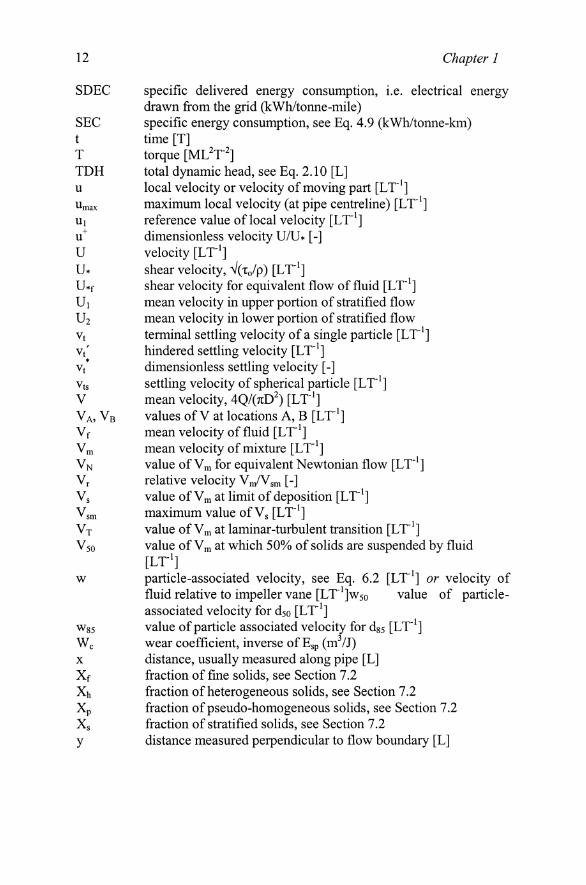
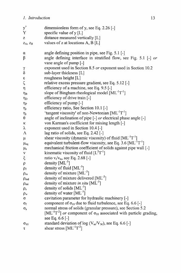
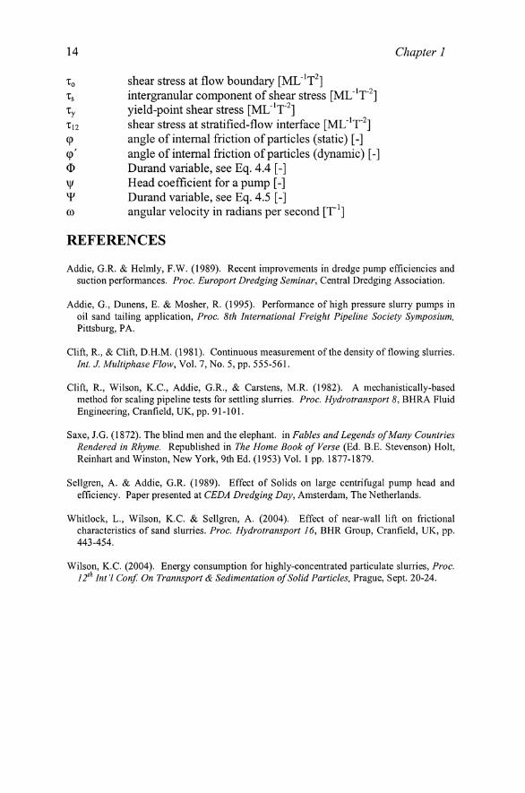
1.3 List of Symbols

The principal symbols used in this book are listed here, together with brief definitions. The basic units of each quantity in terms of mass [M] length [L] and time [T] are given in square brackets. Dimensionless quantities are indicated by [-].

a celerity of transient disturbance [LT^] A' coefficient in Eq. 4.3 [-]. The case where A'= 1.0 is the

equivalent-fluid model Ap maximum projected area of a particle, see Eq. 2.66 [L ]̂ b breadth between pump shrouds [L] B coefficient in Eq. 4.6, dependent on flow stratification [-] Cm absolute fluid veloci ty in meridional direction [LT"^] Cr absolute fluid veloci ty in radial direction [LT"^] Ct absolute fluid veloci ty in tangential direction [LT"^] C D part icle drag coefficient, see Eq. 2.50 [-] Cr relative volumetr ic concentrat ion of solids, Cyd/Cvb [-] Crm value of Cr at wh ich deposi t ion veloci ty is a m a x i m u m [-] Cv volumetr ic concentra t ion (volume fraction) of solids [-] Cvb volumetr ic solids concentrat ion in loose-poured bed [-] Cvd del ivered volumetr ic solids concentrat ion, see Section 2.4 [-] Cvi in situ volumetric solids concentration, see Section 2.4 [-] Cw solids concentration by weight (or mass) [-]

10 Chapter 1

d particle diameter [L] d* dimensionless particle diameter, see Eq. 2.57 [-] da area-equivalent particle diameter, see Eq. 2.66 [L] dso mass-median particle diameter [L] dgs diameter for which 8 5 % (by mass) of the particles are finer [L] D diameter (internal diameter of a pipe, diameter of a pump

impeller) [L] Ds pump suction diameter [L] E voltage [V] Ei energy coefficient for specific impact wear (J/m^) Esp energy coefficient for specific wear (J/m^) f Moody friction factor, see Eq. 2.29 [-] ff value of f for equal volumetric flow of fluid [-] fw value of f for equal volumetric flow of water [-] f 12 value of f at stratified-flow interface [-] fn ( ) a function F D drag force [MLT"^] F L lift force [MLT'^] FN normal intergranular force against pipe wall [MLT'^] Fw immersed weight force [MLT^] g gravitational acceleration [LT^] G coefficient in Eq. 3.18 h height [L] ha atmospheric head (in height of liquid being pumped) [L] hv vapour-pressure head [L] H head, see Eq. 2.9 [L] H A , H B head at locations. A, B . [L] Hi theoretical head, see Eq. 9.10 [L] Hr head ratio, see Section 10.1 [-] Hs suction head [L] i hydraulic gradient [height of water/length of pipe] see Eq. 2.44 if value of i for equal volumetric flow of fluid [height of

water/length of pipe] im value of i for flow of mixture [height of water/length of pipe] imh value of i for flow of homogeneous mixture [height of

water/length of pipe] ipg hydraulic gradient for plug flow, see Eq. 5.8 [height of

water/length of pipe]

i average hydraulic gradient in ascending and descending vertical

flows [height of water/length of pipe]

7. Introduction 11

iw value of i for equal volumetric flow of water [height of water/length of pipe]

iw' hydraulic gradient in return water line [height of water/length of pipe]

I electric current [A] jm friction gradient in height of mixture/length of pipe, see Eq. 2.45 k coefficient in power-law rheological model K volumetric shape factor of particles (Eq. 2.67) [-] or McElvain's,

head-reduction coefficient (Eq. 10.3) [-] L length, measured along pipe [L] m exponent in Eq. 3.18 [-] M exponent in stratification-ratio equation [-] n angular speed in revolutions per second [T^] or Richardson-

Zaki exponent, see Eq. 2.69 [-] or exponent in power-law rheological model [-]

n ' Rabinowitsch-Mooney exponent [-] ns dimensionless specific speed, see Eq. 9.14 [-] N angular speed in revolutions per minute Ns specific speed in customary units, see Eq. 9.15 NPSH net positive suction head, see Eq. 9.16 [L] p pressure [ML'^T"^] PA, PB pressure at locations A, B. [ML'^T'^] Pv vapour pressure [ML'^T^] P power [ML^T-^] Q volumetric flow rate [L^T^] QBEP flow rate at best efficiency point [L^T'^] Qf volumetric flow rate of fluid [L^T"^] Qm volumetric flow rate of mixture [L^T"^] Qs volumetric flow rate of solids [L^T^] r radius [L] RH head reduction factor, see Eq. 10.3 [-] RT3 representative shell radius, see Fig. 11.4 [L] Rr| efficiency reduction factor, see Eq. 10.3 [-] Re Reynolds number VD/v [-] Re* shear Reynolds number U*D/v [-] RCp particle Reynolds number Vtd/v [-] Sf relative density of fluid [-] Sm relative density of mixture [-] Smd delivered relative density of mixture [-] Smi in situ relative density of mixture [-] Ss relative density of solids [-]

12 Chapter 1

SDEC specific delivered energy consumption, i.e. electrical energy drawn from the grid (kWh/tonne-mile)

SEC specific energy consumption, see Eq. 4.9 (kWh/tonne-km) t time [T] T torque [MVT^]

TDH total dynamic head, see Eq. 2.10 [L] u local velocity or velocity of moving part [LT^] Umax m a x i m u m local velocity (at pipe centreline) [LT"^] Ui reference value of local velocity [LT'^] u^ dimensionless velocity U/U* [-] U velocity [LT^] U* shear velocity, V(To/p) [LT^] U*f shear velocity for equivalent flow of fluid [LT^] Ui mean velocity in upper port ion of stratified flow U2 mean velocity in lower portion of stratified flow Vt terminal settling velocity of a single particle [LT^] Vt' hindered settling velocity [LT^] Vt dimensionless settling velocity [-] Vts settling velocity of spherical particle [LT^] V mean velocity, 4Q/(7iD^) [LT^] V A , V B values of V at locations A, B [LT^] Vf mean velocity of fluid [LT'^] Vm mean velocity of mixture [LT"^] V N value of V ^ for equivalent Newtonian flow [LT^] Vr relative velocity VmA^sm [-] Vs value of V ^ at limit of deposition [LT^] Vsm m a x i m u m value of Vs [LT^] V T value of V ^ at laminar-turbulent transition [LT^] V50 value of Vm at which 5 0 % of solids are suspended by fluid

[LT-'] w particle-associated velocity, see Eq. 6.2 [LT^] or velocity of

fluid relative to impeller vane [LT'^Jwso value of particle-associated velocity for dso [LT'^]

W85 value of part icle associated veloci ty for dss [LT"^] Wc wear coefficient, inverse ofEsp(mVj) x distance, usually measured along pipe [L] Xf fraction of fine solids, see Section 7.2 Xh fraction of heterogeneous solids, see Section 7.2 Xp fraction of pseudo-homogeneous solids, see Section 7.2 Xs fraction of stratified solids, see Section 7.2 y distance measured perpendicular to flow boundary [L]

1. Introduction 13

y^ dimensionless form of y, see Eq. 2.26 [-] Y specific value of y [L] z distance measured vertically [L] ZA, ZB values of z at locations A , B [L]

a angle defining posit ion in pipe, see Fig. 5.1 [-] ß angle defining interface in stratified flow, see Fig. 5.1 [-] or

vane angle of p u m p [-] y exponent used in Section 8.5 or exponent used in Section 10.2 5 sub-layer thickness [L] 8 roughness height [L] ^ relative excess pressure gradient, see Eq. 5.12 [-] r| efficiency of a machine , see Eq. 9.5 [-] T]B slope of B ingham rheological model [ML'^T^] TjD efficiency of drive train [-] Tjp efficiency of pump [-] r|r efficiency ratio. See Section 10.1 [-] r|t 'tangent viscosity' of non-Newtonian [ML'^T^] 0 angle of inclination of pipe [-] or electrical phase angle [-] K von Karman's coefficient for mixing length [-] X exponent used in Section 10.4 [-] A lag ratio of sohds, see Eq. 2.42 [-] |i shear viscosity (d3mamic viscosity) of fluid [ML'̂ T"^] |Lieq equivalent turbulent-flow viscosity, see Eq. 3.6 [ML'^T^] |Lis mechanical friction coefficient of solids against pipe wall [-] V kinematic viscosity of fluid [L^T^] ^ ratio v/vts, see Eq. 2.68 [-] p density [ML"^] pf density of fluid [ML"^] pm density of mixture [ML'^] pmd density of mixture delivered [ML'^] pmi density of mixture in situ [ML"^] Ps density of solids [ML"^] pw density of water [ML'^ ] G cavitation parameter for hydraulic machinery [-] Of component of GIO due to fluid turbulence, see Eq. 6.6 [-] Gs normal stress of sohds (granular pressure) , see Section 5.2

[ML'^T'^] or component of GIO associated with particle grading, see Eq. 6.6 [-]

Gio standard deviation of log (VmA^so), see Eq. 6.6 [-] T shear stress [ML'^T^]

14 Chapter 1

To shear stress at f low bounda ry [ML'^T^] Ts in tergranular c o m p o n e n t of shear stress [ML'^T"^] Xy yield-point shear stress [ML'^T^] Ti2 shear stress at stratified-flow interface [ML'^T"^] (p angle of internal friction of particles (static) [-] cp' angle of internal friction of particles (dynamic) [-] O Durand variable, see Eq. 4.4 [-] \|/ Head coefficient for a pump [-] ^ Durand variable, see Eq. 4.5 [-] (0 angular velocity in radians per second [T^]

REFERENCES

Addle, G.R. & Helmly, F.W. (1989). Recent improvements in dredge pump efficiencies and suction performances. Proc. Europort Dredging Seminar, Central Dredging Association.

Addie, G., Dunens, E. & Mosher, R. (1995). Performance of high pressure slurry pumps in oil sand tailing application, Proc. 8th International Freight Pipeline Society Symposium, Pittsburg, PA.

Clift, R., & Clift, D.H.M. (1981). Continuous measurement of the density of flowing slurries. Int. J. Multiphase Flow, Vol. 7, No. 5, pp. 555-561.

Clift, R., Wilson, K.C., Addie, G.R., & Carstens, M.R. (1982). A mechanistically-based method for scaling pipeline tests for settling slurries. Proc. Hydrotransport 8, BHRA Fluid Engineering, Cranfield, UK, pp. 91-101.

Saxe, J.G. (1872). The blind men and the elephant, in Fables and Legends of Many Countries Rendered in Rhyme. Republished in The Home Book of Verse (Ed. B.E. Stevenson) Holt, Reinhart and Winston, New York, 9th Ed. (1953) Vol. 1 pp. 1877-1879.

Sellgren, A. & Addie, G.R. (1989). Effect of Solids on large centrifugal pump head and efficiency. Paper presented at CEDA Dredging Day, Amsterdam, The Netherlands.

Whitlock, L., Wilson, K.C. & Sellgren, A. (2004). Effect of near-wall lift on frictional characteristics of sand slurries. Proc. Hydrotransport 16, BHR Group, Cranfield, UK, pp. 443-454.

Wilson, K.C. (2004). Energy consumption for highly-concentrated particulate slurries, Proc. 12^^ Int'l Conf. On Trannsport & Sedimentation of Solid Particles, Prague, Sept. 20-24.

2. Review of Fluid and Particle Mechanics

Chapter 2

REVIEW OF FLUID AND PARTICLE MECHANICS

2.1 Introduction

Before considering the flow of mixtures of liquids and solid particles, we must first treat the flow of single-phase liquids and the motion of particles in liquids. These topics also provide an introduction to concepts, terminology and notation used in later chapters. The treatment in this chapter is at the level of a review, intended primarily to reinforce knowledge which readers will have encountered in their undergraduate engineering curriculum, but may have not utilized in the interim. As in other parts of this book, the level of presentation is directed to practical engineering application. This chapter is not intended as an introduction to fluid mechanics in general, to turbulence, or to the micromechanics of particle-fluid systems. All these subjects have significance for fundamental research, but they are not required for an engineering treatment of slurry flow.

To characterise a simple fluid such as water only two material properties are required: density and viscosity. The density, denoted by p, represents the mass of fluid per unit volume. The viscosity is a measure of the resistance of the fluid to deformation by shearing, and is best illustrated by reference to a conceptual experiment illustrated in Fig. 2.1. The fluid fills a gap of

16 Chapter 2

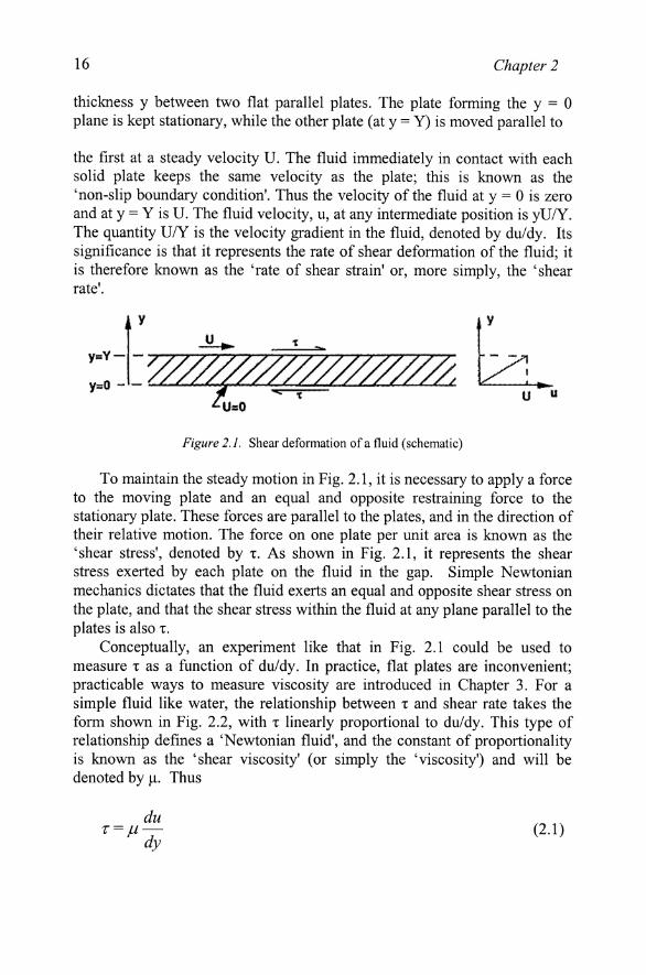
thickness y between two flat parallel plates. The plate forming the y = 0 plane is kept stationary, while the other plate (at y = Y) is moved parallel to

the first at a steady velocity U. The fluid immediately in contact with each solid plate keeps the same velocity as the plate; this is known as the 'non-slip boundary condition'. Thus the velocity of the fluid at y = 0 is zero and at y = Y is U. The fluid velocity, u, at any intermediate position is ylJ/Y. The quantity U/Y is the velocity gradient in the fluid, denoted by du/dy. Its significance is that it represents the rate of shear deformation of the fluid; it is therefore known as the 'rate of shear strain' or, more simply, the 'shear rate'.

- y//////////////7z^/. Figure 2.7. Shear defomiation of a fluid (schematic)

To maintain the steady motion in Fig. 2.1, it is necessary to apply a force to the moving plate and an equal and opposite restraining force to the stationary plate. These forces are parallel to the plates, and in the direction of their relative motion. The force on one plate per unit area is known as the 'shear stress', denoted by x. As shown in Fig. 2.1, it represents the shear stress exerted by each plate on the fluid in the gap. Simple Newtonian mechanics dictates that the fluid exerts an equal and opposite shear stress on the plate, and that the shear stress within the fluid at any plane parallel to the plates is also x.

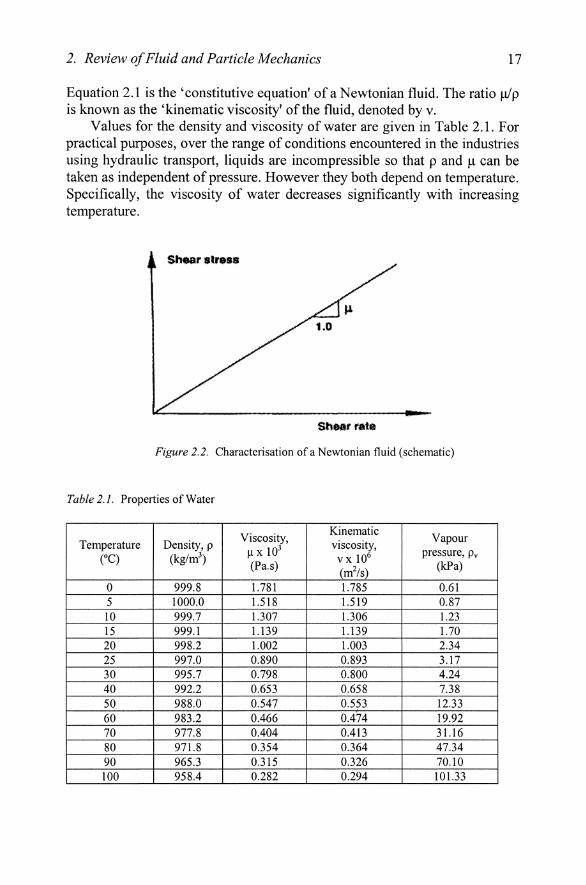
Conceptually, an experiment like that in Fig. 2.1 could be used to measure x as a function of du/dy. In practice, flat plates are inconvenient; practicable ways to measure viscosity are introduced in Chapter 3. For a simple fluid like water, the relationship between x and shear rate takes the form shown in Fig. 2.2, with x linearly proportional to du/dy. This type of relationship defines a 'Newtonian fluid', and the constant of proportionality is known as the 'shear viscosity' (or simply the 'viscosity') and will be denoted by |LI. Thus

1^ du

dy (2.1)

2. Review of Fluid and Particle Mechanics 17

Equation 2.1 is the 'constitutive equation* of a Newtonian fluid. The ratio |a/p is known as the 'kinematic viscosity' of the fluid, denoted by v.

Values for the density and viscosity of water are given in Table 2.1. For practical purposes, over the range of conditions encountered in the industries using hydraulic transport, Hquids are incompressible so that p and |LI can be taken as independent of pressure. However they both depend on temperature. Specifically, the viscosity of water decreases significantly with increasing temperature.

Shsar %Xtwm

W^mm rut«

Figure 2.2. Characterisation of a Newtonian fluid (schematic)

Table 2.1. Properties of Water

Temperature CO

0 5 10 15 20 25 30 40 50 60 70 80 90 100

Density, p (kg/m^)

999.8 1000.0 999.7 999.1 998.2 997.0 995.7 992.2 988.0 983.2 977.8 971.8 965.3 958.4

Viscosity, ^xlO^ (Pa.s)

1.781 1.518 1.307 1.139 1.002 0.890 0.798 0.653 0.547 0.466 0.404 0.354 0.315 0.282

Kinematic viscosity, vxlO^ (mVs) 1.785 1.519 1.306 1.139 1.003 0.893 0.800 0.658 0.553 0.474 0.413 0.364 0.326 0.294

Vapour pressure, Pv

(kPa)

0.61 0.87 1.23 1.70 2.34 3.17 4.24 7.38 12.33 19.92 31.16 47.34 70.10 101.33

18 Chapter 2

2.2 Basic Relations for Flow of Simple Fluids

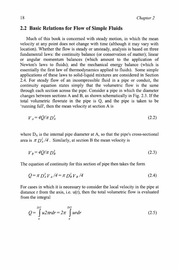
Much of this book is concerned with steady motion, in which the mean velocity at any point does not change with time (although it may vary with location). Whether the flow is steady or unsteady, analysis is based on three fundamental laws: the continuity balance (or conservation of matter); linear or angular momentum balances (which amount to the application of Newton's laws to fluids); and the mechanical energy balance (which is essentially the first law of thermodynamics applied to fluids). Some simple applications of these laws to solid-liquid mixtures are considered in Section 2.4. For steady flow of an incompressible fluid in a pipe or conduit, the continuity equation states simply that the volumetric flow is the same through each section across the pipe. Consider a pipe in which the diameter changes between sections A and B, as shown schematically in Fig. 2.3. If the total volumetric flowrate in the pipe is Q, and the pipe is taken to be 'running full', then the mean velocity at section A is

VA-4Q/7rD'A (2.2)

where DA is the internal pipe diameter at A, so that the pipe's cross-sectional area is n D\/4 . Similarly, at section B the mean velocity is

VB = 4Q/7rDl (2.3)

The equation of continuity for this section of pipe then takes the form

Q^^DAVA/^^TTDIVB /4 (2.4)

For cases in which it is necessary to consider the local velocity in the pipe at distance r from the axis, i.e. u(r), then the total volumetric flow is evaluated from the integral

D/2 D/2

Q= \ u2nrdr = 271 \ urdr (2.5)

2. Review of Fluid and Particle Mechanics 19

in which the area of the element from r to (r+dr) is 27crdr and the velocity through it is u. Specific applications of Eq. 2.5 are considered below, and in Chapter 3.

i

i_j "XL f I I I

Figure 2.3. Flow in a pipe with change in diameter (schematic)

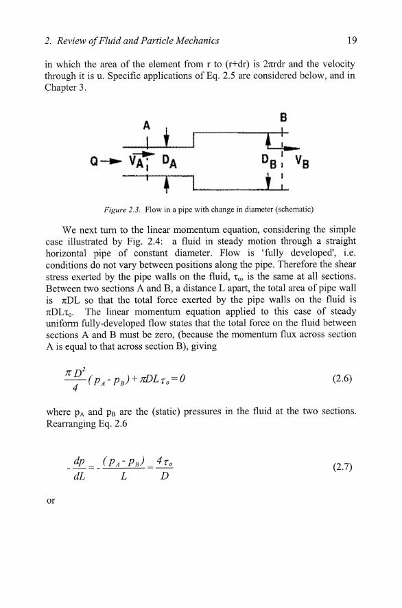
We next turn to the linear momentum equation, considering the simple case illustrated by Fig. 2.4: a fluid in steady motion through a straight horizontal pipe of constant diameter. Flow is 'fully developed', i.e. conditions do not vary between positions along the pipe. Therefore the shear stress exerted by the pipe walls on the fluid, Xo, is the same at all sections. Between two sections A and B, a distance L apart, the total area of pipe wall is TcDL so that the total force exerted by the pipe walls on the fluid is TCDLTQ. The linear momentum equation applied to this case of steady uniform fully-developed flow states that the total force on the fluid between sections A and B must be zero, (because the momentum flux across section A is equal to that across section B), giving

^(PA-PB) + ̂ Lro-0 (2.6)

where PA and pß are the (static) pressures in the fluid at the two sections. Rearranging Eq. 2.6

dp^^ (PA-PB) ^4T,

dL ' L D

or

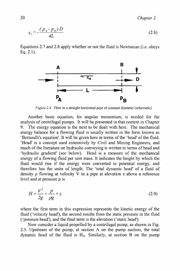
20 Chapter 2

r . ' - ' - ^ ^ ^ (2.8) 4L

Equations 2.7 and 2.8 apply whether or not the fluid is Newtonian (i.e. obeys Eq.2.1).

m

i D

f ^ y B.

Figure 2.4. Flow in a straight horizontal pipe of constant diameter (schematic)

Another basic equation, for angular momentum, is needed for the analysis of centrifugal pumps. It will be presented in that context in Chapter 9. The energy equation is the next to be dealt with here. The mechanical energy balance for a flowing fluid is usually written in the form known as 'Bernoulli's equation'. It will be given here in terms of the 'head' of the fluid. 'Head' is a concept used extensively by Civil and Mining Engineers, and much of the literature on hydraulic conveying is written in terms of head and 'hydraulic gradient' (see below). Head is a measure of the mechanical energy of a flowing fluid per unit mass. It indicates the height by which the fluid would rise if the energy were converted to potential energy, and therefore has the units of length. The 'total dynamic head' of a fluid of density p flowing at velocity V in a pipe at elevation z above a reference level and at pressure p is

H = — + -^ + z (2.9) 2g pg

where the first term in this expression represents the kinetic energy of the fluid ('velocity head'), the second results from the static pressure in the fluid ('pressure head'), and the final term is the elevation ('static head').

Now consider a liquid propelled by a centrifugal pump, as shown in Fig. 2.5. Upstream of the pump, at section A on the pump suction, the total dynamic head of the fluid is HA- Similarly, at section B on the pump

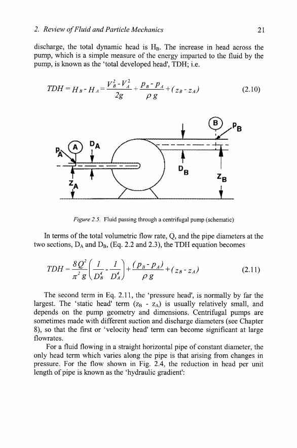
2. Review of Fluid and Particle Mechanics 21

discharge, the total dynamic head is Hß. The increase in head across the pump, which is a simple measure of the energy imparted to the fluid by the pump, is known as the 'total developed head', TDH; i.e.

TDH = HB-H, Vl

2g

Vl ^PB-PA

Pg + ( ZB " ZAy (2.10)

Figure 2.5. Fluid passing through a centrifugal pump (schematic)

In terms of the total volumetric flow rate, Q, and the pipe diameters at the two sections, DA and Dß, (Eq. 2.2 and 2.3), the TDH equation becomes

TDH _8Q ^ (

n g D'B D\.

(PB-PA)

pg + ( ZB~ ZA^ (2.11)

The second term in Eq. 2.11, the 'pressure head', is normally by far the largest. The 'static head* term (ZB - ZA) is usually relatively small, and depends on the pump geometry and dimensions. Centrifugal pumps are sometimes made with different suction and discharge diameters (see Chapter 8), so that the first or 'velocity head' term can become significant at large flowrates.

For a fluid flowing in a straight horizontal pipe of constant diameter, the only head term which varies along the pipe is that arising from changes in pressure. For the flow shown in Fig. 2.4, the reduction in head per unit length of pipe is known as the 'hydraulic gradient':

22

: _ (PA-PB) _ 4 To

PgL pgD

Chapter 2

(2.12)

Here i has been related to the wall shear stress, Xo, using Eq. 2.7. The units of the hydraulic gradient are (m head lost)/(m pipe run), or feet of head per foot of pipe. Thus the numerical value of i is independent of the system of units used. However, i is not strictly a dimensionless number: for example, if the flow took place on the moon or in any other environment of changed gravity, the value of i would be different even though TQ and the pressure gradient were unchanged.

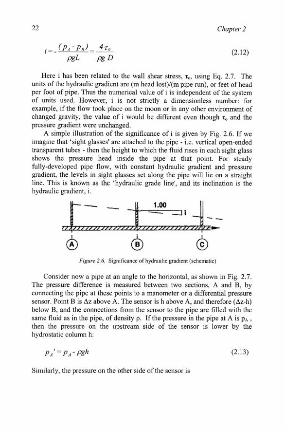
A simple illustration of the significance of i is given by Fig. 2.6. If we imagine that 'sight glasses' are attached to the pipe - i.e. vertical open-ended transparent tubes - then the height to which the fluid rises in each sight glass shows the pressure head inside the pipe at that point. For steady fully-developed pipe flow, with constant hydraulic gradient and pressure gradient, the levels in sight glasses set along the pipe will lie on a straight line. This is known as the 'hydraulic grade line', and its inclination is the hydraulic gradient, i.

1.00

^/|///ZZ///////////f////////^/7?////4'

(A) (5) ^

Figure 2.6. Significance of hydraulic gradient (schematic)

Consider now a pipe at an angle to the horizontal, as shown in Fig. 2.7. The pressure difference is measured between two sections, A and B, by connecting the pipe at these points to a manometer or a differential pressure sensor. Point B is Az above A. The sensor is h above A, and therefore (Az-h) below B, and the connections from the sensor to the pipe are filled with the same fluid as in the pipe, of density p. If the pressure in the pipe at A is PA , then the pressure on the upstream side of the sensor is lower by the hydrostatic column h:

PA=P, pgh (2.13)

Similarly, the pressure on the other side of the sensor is