Slotting Allowances and Conditional Payments∗

Patrick Rey† Jeanine Thal‡ Thibaud Vergé§

July 27, 2006

Abstract

We analyze the competitive effects of upfront payments made by manufactur-

ers to retailers in a contracting situation where rival retailers offer contracts to a

manufacturer. In contrast to Bernheim and Whinston (1985, 1998), who study the

situation in which competing manufacturers offer contracts to a common retailer,

we find that two-part tariffs (even if contingent on exclusivity or not) do not suffice

to implement the monopoly outcome. More complex arrangements are required to

internalize all the contracting externalities. The retailers can for example achieve

the monopoly outcome through (contingent) three-part tariffs that combine slotting

allowances (i.e., upfront payments by the manufacturer) with two-part tariffs where

the fees are conditional on actual trade. The welfare implications are ambiguous.

On the one hand, slotting allowances ensure that no efficient retailer is excluded.

On the other hand, they allow firms to maintain monopoly prices in a common

agency situation. Simulations suggest that the latter effect is more significant.

Keywords: Vertical contracts, slotting allowances, buyer power, common agency

JEL classification codes: L14, L42.

∗We would like to thank Mike Whinston, David McAdams, Lucy White and participants at the 3rd

International Industrial Organization Conference (Atlanta), ESSET 2005 (Gerzensee), CEPR Compe-

tition Policy and International Trade Conference (Brussels), 7th INRA-IDEI Conference on “Industrial

Organization and the Agro-Food Industry”(Toulouse) and seminars at Mannheim, University of East

Anglia, CREST-LEI and Toulouse for useful comments.†University of Toulouse (IDEI and GREMAQ), prey@cict.fr‡CREST—LEI and University of Toulouse (GREMAQ), JeanineThal@gmail.com§CREST—LEI, thibaud.verge@ensae.fr

1

1 Introduction

In recent years, payments made by manufacturers to retailers have triggered heated de-

bates.1 The term slotting allowance usually encompasses different kinds of such payments:

slotting fees for access to (sometimes premium) shelf space, advertising fees for promo-

tional activities, fees related to the introduction of new products, or listing and pay-to-stay

fees that suppliers pay to be or remain on the retailer’s (formal or informal) list of poten-

tial suppliers. Such payments are not negligible: according to a recent study published

by the FTC (2003), “for those products with slotting allowances, the average amount of

slotting allowances (per item, per retailer, per metropolitan area) for all five categories

combined ranged from $2,313 to $21,768. (...) Most of the surveyed suppliers reported

that a nationwide introduction of a new grocery product would require $1.5 to $2 million

in slotting allowances.”

In France, manufacturers have long been complaining about the growing magnitude of

slotting allowances and hidden margins, and these practices have been at the center of the

debate about the 2005 reform of the 1996 Galland Act. Splitting the total margin made

by a retailer on a product into the observable margin (which includes all rebates written

on the original invoice and the retailer’s margin) and the hidden margin (which includes

negotiated slotting allowances and conditional rebates such as listing fees paid at the end

of the year), Allain and Chambolle (2005) claim that the hidden margin represented on

average 88 percent of the total margin made by French supermarkets on grocery products

in 1999.

While pro-competitive justifications have been brought forward for fees related to the

allocation of shelf space, advertising or the introduction of new products,2 listing or pay-

to-stay fees are particularly contentious.3 In the UK for example, where 58 percent of

large suppliers reported in 2000 that major supermarket chains requested listing fees,4

1See for example the reports by the FTC (2001) in the U.S. or the Competition Commission (2000)

in the U.K..2Slotting fees are often considered to be an efficient way to allocate scarce shelf space (however, there is

some concern that large manufacturers may use such fees to exclude smaller competitors whose pockets

are not deep enough to match such offers — see Bloom et al. (2000), and Shaffer (2005) for a formal

analysis).3Fees related to promotional activities can be a way to compensate a retailer for additional effort (see

e.g. Klein-Wright (2006)). Fees related to the introduction of a new product may serve risk-sharing,

signaling or screening purposes (see Kelly (1991)).4See Table 11.5 of the report by the Competition Commission (2000).

2

the supermarkets code of practice introduced in 2001 prohibits lump sum fees not related

to promotional activities or to the introduction of a new product (a recent report shows,

however, that listing fees continue to be common).5

The economic literature on listing fees and more generally on slotting allowances has

first focused on manufacturers’ incentives to offer such payments. Shaffer (1991) shows

that even perfectly competitive manufacturers can dampen retail competition by offer-

ing wholesale prices above marginal cost and compensate retailers by means of slotting

allowances. Yet, in the grocery industry for example, the general perception is that bar-

gaining power has shifted towards large retail chains in recent years.6 Large supermarket

chains often account for a high share of a manufacturer’s production: in the UK, even

large manufacturers typically rely on their main buyer for more than 30 percent of do-

mestic sales. In contrast, the business of a leading manufacturer usually represents a very

small proportion of business for each of the major multiples. Finally, while large manu-

facturers certainly continue to possess a strong bargaining position on some must-stock

brands, this strength does not necessarily carry over to other goods, since negotiations

mostly take place on a product-by-product basis.7

Real-world evidence indicates that both the incidence and the magnitude of slotting

allowances are associated with the exercise of retail bargaining power.8 To capture this

idea, Marx and Shaffer (2004) consider a model of vertical negotiations where retailers

have the initiative and show that strong retailers can exclude other retailers by offering

“three-part tariffs” that include upfront payments (slotting allowances), paid by the man-

ufacturer even if the retailer does not buy anything afterwards, and conditional fixed fees,

paid by the retailer only if it actually buys from the manufacturer.

Building on their analysis, we find that retailers may in fact use upfront payments

and conditional fixed fees to achieve monopoly profits when distributing the good of a

common supplier. As in Marx and Shaffer (2004), we consider a situation where rival,

differentiated retailers offer public take-it-or-leave-it contracts to a single manufacturer;

however, we allow contracts to be contingent on whether the retailer gets exclusivity or5See Office of Fair Trading (2004).6See Inderst and Wey (2006) for more evidence on the retailers’ growing bargaining power in different

sectors both in Europe and in the US.7See the supermarket report published by the Competition Commission (2000).8See the FTC (2001) staff report for instance. The Competition Commission (2000) states that “some

suppliers said that they regarded these charges as exploitation of the power differences between the retailer

and the supplier.”

3

not. This assumption can be motivated in two ways. First, one might indeed expect firms

to discuss what would be the terms for both options. Second, even when firms negotiate a

non-contingent contract, they do so with a given market configuration in mind, and would

probably renegotiate the terms of the contract if the actual configuration turned out not

to be as expected.9 We study in this context the role of conditional fixed fees and upfront

payments in determining: (i) whether exclusion is a profitable strategy for a retailer, and

(ii) the levels of prices when both retailers distribute the good. We show that there exist

equilibria where firms achieve the integrated monopoly outcome, and that the retailers’

preferred equilibrium gives each retailer its entire contribution to the industry monopoly

profits.

If it had the bargaining power, the manufacturer could sustain the industry monopoly

outcome even without slotting allowances or conditional fees: it could simply offset the

competitive pressure on retail prices by charging wholesale prices above costs, so as to

maintain consumer prices at the monopoly level, and recover any remaining retail profit

through fixed fees. When the retailers have the initiative, however, standard two-part

tariffs no longer yield monopoly prices and profits when both retailers are active, since

each retailer then has an incentive to free-ride on its rival’s revenue by reducing its own

price. By reducing the profits that can be achieved, this free-riding may moreover lead to

the exclusion of a retailer.

In this context, conditioning fixed fees on actual trade contributes to protect retailers

against such free-riding, since they can then “opt out” and waive the fixed fee if a rival tries

to undercut them. Combined with upfront payments by the manufacturer, conditional

fixed fees then allow retailers to be both active and achieve the industry monopoly profits:

wholesale prices above costs maintain retail prices at the monopoly level, while large

conditional payments (up to the retailers’ anticipated variable profits) protect retailers

against any opportunistic move by their rivals. Upfront payments by the manufacturer

can then be used to give ex ante each retailer its contribution to the industry profits.

Last, each retailer can discourage its rivals from deviating to exclusivity by adjusting the

terms of its own exclusive dealing offer. Thus, when combined with conditional fixed

fees, upfront payments do not lead to inefficient exclusion but may actually avoid it. Yet,

upfront payments are still potentially detrimental for welfare, since they eliminate any

effective retail competition.9Indeed, contracts often stipulate a clause triggering renegotiation in case of a “material change in

circumstances.”

4

Incidentally, our analysis supports the view that slotting allowances are associated

with retail bargaining power.10 If bargaining power were upstream, the industry monopoly

outcome could be achieved without slotting allowances; standard two-part tariffs would

suffice. Once retailers have the bargaining power, however, upfront payments are neces-

sary to maintain monopoly prices.

Our paper is related to the literature on contracting with externalities. Bernheim and

Whinston (1985) show that manufacturers can use a common agent to coordinate and

achieve monopoly prices. Bernheim and Whinston (1998) examine the case of a monop-

olistic retailer and analyze whether a manufacturer can exclude a rival from distribution,

when the initiative to offer contracts lies upstream. Because of the compensation required

by the retailer, and in the absence of any specific contracting externalities, exclusion does

not occur and standard (non-contingent) two-part tariffs suffice to achieve the industry

monopoly outcome. Contracting externalities could arise for example from a restriction

on contracts,11 or from third parties not present at the contracting stage.12 In contrast,

in our setting where competing retailers offer contracts to a common supplier, simple

two-part tariffs (even if contingent on exclusivity or not) do not suffice to implement the

monopoly outcome; more complex arrangements, such as contingent three-part tariffs are

required to internalize all the contracting externalities.

More recently, Martimort and Stole (2003) as well as Segal and Whinston (2003) have

analyzed bidding games where rival retailers simultaneously offer supply contracts to a

monopolist manufacturer. They find that both retailers may be active in equilibrium but

there always remains some retail competition; the outcome is therefore always inefficient

from the firms’ point of view. As we will see later on, the key assumptions explaining the

differences between their results and ours are that, although tariffs are offered in both

cases by the downstream firms (who thus have the bargaining power), in their setup:

(i) quantities are chosen by the upstream firm, which limits retailers’ ability to protect

themselves against rivals’ opportunistic moves; and (ii) contracts cannot be contingent10Inderst (2005) also looks at the role of buyer power and slotting allowances, but in a context where

manufacturers supply a monopolist retailer. He shows that, when the retailer has a weak bargaining

power vis-à-vis the manufacturers, the retailer might find it desirable to commit ex ante to exclusivity

(and transform de facto upstream competition into an auction where manufacturers bid on slotting

allowances).11For instance, Mathewson and Winter (1987) consider a restriction to linear prices.12For example, an incumbent manufacturer can sometimes profitably prevent efficient entry: see Aghion

and Bolton (1987), Rasmusen et al. (1991), Segal and Whinston (2000) and Comanor and Rey (2000).

5

on market structure. In the case of relationships between manufacturers and retailers,

it may however be more realistic to postulate that the downstream firms are the ones

choosing how much to procure.

The paper is organized as follows. Section 2 outlines the general framework. Section 3

derives upper bounds on retailers’ rents, which will serve as benchmarks in the following

analysis. Sections 4 to 6 consider different classes of contracts: classic two-part tariffs with

an upfront fixed fee, two-part tariffs with a conditional fixed fee and finally three-part

tariffs combining both types of fees. Section 7 links our results to the existing literature

and discusses the policy implications of our findings. The final section concludes.

2 Framework

Two differentiated retailers, R1 and R2, distribute the product of a manufacturerM . The

manufacturer produces at constant marginal cost c, while retailers incur no additional

distribution costs. Retailers have all the bargaining power in their bilateral relations with

the manufacturer; their interaction is therefore modeled as follows:

1. R1 and R2 simultaneously make take-it-or-leave-it offers to M . Offers can be con-

tingent on exclusivity, that is, each retailer Ri offers a pair of contracts¡CCi , C

Ei

¢where CCi and C

Ei respectively specify the terms of trade when the manufacturer

has accepted both offers or Ri’s offer only.13 The offers are thus only contingent on

acceptance decisions.

2. M decides whether to accept both, only one, or none of the offers. All offers and

acceptance decisions are public.

3. The retailers with accepted contracts compete on the downstream market and the

relevant contracts are implemented.

We do not specify how competition takes place on the retail market; in particular,

our results are valid for quantity as well as price competition. Denoting by Pi (qi, q−i)

the inverse demand function at store i = 1, 2 when Ri sells qi units of the good and R−i

sells q−i units,14 we denote by Πm the maximum profit that can be achieved by a fully13Throughout the paper, superscripts C and E respectively refer to common agency and exclusive

dealing situations.14Throughout the paper, the notation “−i” refers to retailer i’s rival.

6

integrated firm:

Πm = max(q1,q2)

{(P1 (q1, q2)− c) q1 + (P2 (q2, q1)− c) q2} .

When only product i is available, a vertically integrated firm (including M and Ri) max-

imizing its profit would earn:

Πmi = maxqi{(Pi (qi, 0)− c) qi} .

We assume that the two retailers are imperfect substitutes and, without loss of generality,

that R1 on its own is at least as profitable as R2, that is:

Πm1 +Πm2 > Πm > Πm1 ≥ Πm2 .

At this point, let us discuss the main assumptions underlying our model. First, the

above strict inequalities rule out the cases where the two markets are independent or

the two retailers are perfect substitutes. These two cases would be trivial in our setting:

when the markets are independent, two-part tariffs would suffice to achieve the monopoly

outcome, while exclusive dealing would be efficient (and the associated monopoly profits

easily achieved) when there is perfect substitutability.

Second, we have assumed that contracts are public. Since the manufacturer observes

both offers at stage 1, no problem of opportunism arises vis-à-vis the supplier even when

the retailers cannot observe contracts. However, if retailers did not observe contracts

before competing on the product market, each retailer would have an incentive to free-

ride on the other, thereby limiting the retailers’ ability to avoid competition (see the

discussion in Section 7.1).

Last, as already mentioned, we allow contracts to be contingent on exclusivity. This

reflects the fact that in practice firms may indeed explore both options, and can also

be viewed as a “short-cut” capturing the possibility of renegotiation in case of a refusal

to deal. An alternative approach would be to introduce an explicit dynamic multilateral

framework: this is for example the route followed by de Fontenay and Gans (2005a) who

use the bargaining model developed by Stole and Zwiebel (1996). They consider contracts

that stipulate a given quantity for a given total price, and show that while the outcome

is bilaterally efficient, it fails to maximize the industry profits.15 In our framework,

where contracts will also be bilaterally efficient, rich enough contracts, combining upfront

payments and conditional fixed fees can achieve joint-profit maximization.15De Fontenay and Gans (2005b) use a similar approach to study the impact of vertical integration.

7

3 Common Agency Profits

Before turning to specific contractual relationships, it is useful to derive bounds on the

equilibrium payoffs in common agency situations, that is, in situations where both retailers

are active. We will only assume here that, if retailer R−i is inactive, the pair Ri−M can

achieve and share the bilateral monopoly profit Πmi as desired.16 We denote by ΠC the

equilibrium industry profits under common agency, and by πC1 , πC2 and πCM , respectively,

the retailers’ and the manufacturer’s equilibrium profits. By definition, ΠC cannot exceed

the industry monopoly profits Πm; it may however be lower if contracting externalities

prevent the maximization of industry profits in equilibrium.

In any common agency equilibrium, the joint profits of a given vertical pair Ri −Mmust exceed the bilateral profit it could achieve by excludingR−i: indeed, if πCi + πCM < Πmi ,

then Ri could profitably deviate by offering an exclusive dealing contract generating the

bilateral monopoly profit and leaving a slightly higher payoff to M .17 There is thus no

profitable deviation to exclusivity if and only if Ri andM jointly get at least their bilateral

monopoly profit: for i = 1, 2,

πCi + πCM ≥ Πmi . (1)

This, in turn, implies that a retailer cannot earn more than its contribution to total

profits: since by definition, πCi +πCM = ΠC−πC−i, condition (1) (written for “− i”) impliesthat, for i = 1, 2,

πCi ≤ ΠC −Πm−i. (2)

These upper bounds imply that the manufacturer’s equilibrium payoff πCM is always pos-

itive:

πCM = ΠC − πC1 − πC2

≥ ΠC −¡ΠC −Πm2

¢−¡ΠC −Πm1

¢= Πm1 +Πm2 −ΠC

≥ Πm1 +Πm2 −Πm > 0.

M ’s participation constraint is thus strictly satisfied in any common agency equilibrium.16Standard two-part tariffs, for example, can achieve this. The discussion below parallels that of

Bernheim and Whinston (1998) who consider the case where upstream firms compete for a downstream

monopolist.17For example, a two-part tariff Ti (qi) = Fi + cqi, with Fi just above πCM conditional on exclusivity,

would do.

8

Since individual rationality also requires πCi ≥ 0 for all i, condition (2) implies that a

common agency equilibrium can only exist if it is more profitable than exclusive dealing,

namely if:

ΠC ≥ Πm1 . (3)

In the next three sections, we will successively consider two-part tariffs with upfront

fees (paid either by or to the manufacturer), two-part tariffs with conditional fixed fees

(paid only in case of actual trade) and three-part tariffs (combining upfront and condi-

tional fixed fees) and look at the conditions under which the inequality (3) is satisfied.

This will also allow us the identify the exact roles played by the different types of fixed

fees (upfront or conditional).

4 Two-Part Tariffs

Bernheim and Whinston (1985, 1998) have shown that, when rival manufacturers deal

with a common retailer, simple two-part tariffs that consist of a constant wholesale price

and a fixed fee suffice to maximize industry profits. Although they focused on the case

where manufacturers have the bargaining power in their bilateral relations with the com-

mon agent, their conclusions remain valid when the retailer has the initiative: in both

instances, the retailer plays the role of a “gatekeeper” for consumers and fully internalizes,

through marginal cost pricing, any contracting externalities.18

This result remains valid when rival retailers deal with a common supplier, provided

that it is the supplier that chooses the terms of the contracts. By setting wholesale prices

at the right level above marginal cost, the supplier can induce retailers to set monopoly

prices despite retail competition; the supplier can then use fixed fees to extract retail

profits. As we will see, this result no longer holds when the retailers are the ones that

choose the terms of the contracts. While the supplier can act as a “common agent” for

the retailers, two-part tariffs do not allow them to coordinate fully their pricing decisions,

since each retailer-manufacturer pair has an incentive to free-ride on the other retailer’s

revenues.18This also remains the case when contracts are not publicly observable, contract observability being

irrelevant when the manufacturers are the ones that make the offers. If instead the retailer makes take-

it-or-leave-it offers, it would require the manufacturers to supply at cost and have no incentive to behave

opportunistically (altering one contract cannot hurt the other manufacturer).

9

Furthermore, in the context studied by Bernheim and Whinston, or when a single

manufacturer offers (public) contracts to competing retailers, two-part tariffs need not be

contingent on the set of accepted offers to sustain the common agency equilibrium. In

contrast, Marx and Shaffer (2004) point out that when retailers have the initiative and

offer non-contingent contracts, in any non-exclusive equilibrium the joint profits of the

manufacturer and a retailer are strictly lower than what they could achieve with exclusive

dealing. Indeed, in any candidate common agency equilibrium: (i) the manufacturer

must be indifferent between accepting both offers or only one retailer’s offer, otherwise

that retailer could offer a smaller fixed fee; but (ii) that retailer would be better off if the

manufacturer refused its rival’s offer, since it would receive or pay the same fee but obtain

greater variable profits.19 The retailer thus has an incentive to deviate to an exclusive

dealing situation.20

In the remainder of this section, we therefore consider two-part tariffs that are con-

tingent on exclusivity, of the form:

tki (q) = Uki + w

ki q, for q ≥ 0 and k = C,E .

We derive a necessary and sufficient condition for the existence of a common agency

equilibrium in this context.

Exclusive Dealing

First note that there always exists an exclusive dealing equilibrium. Clearly, if Ri insists

on exclusivity (e.g., by offering only exclusivity, or by degrading its non-exclusive option),

R−i cannot do better than also insist on exclusivity. In addition, if M sells at cost

exclusively to Ri (wi = c, w−i = +∞, say), Ri will maximize its joint profits withM , thusgenerating a total profit equal to Πmi . The fixed fee U

Ei can then be used to share these

profits as desired. As a result:

Lemma 1 There always exists an exclusive dealing equilibrium:

• If Πm1 > Πm2 , in any such equilibrium R1 is the active retailer while R2 gets zero

profit; among these equilibria, the unique trembling-hand perfect equilibrium, which

is also the most favorable to the retailers, yields Πm1 −Πm2 for R1 and Πm2 for M .19Note that retail margins are indeed positive whenever retail competition is imperfect (because of

differentiation, as we assume here, Cournot competition in quantities, ...).20Depending on demand conditions, a standard two-part tariff may suffice to induce exclusivity; oth-

erwise, the contract must include some form of exclusivity provision.

10

• If Πm1 = Πm2 , there exist two exclusive dealing equilibria, where either retailer is

active. In both cases, retailers earn zero profits and M gets Πm2 .

Proof. If one retailer offers only an exclusive dealing contract, then the other retailer

cannot gain by making a non-exclusive offer. Hence, without loss of generality we can

restrict attention to equilibria in which both retailers only offer exclusive dealing contracts.

In any such equilibrium, the joint profits of the manufacturer and the active retailer,

Ri, must be maximized; otherwise Ri could profitably deviate to a different exclusive

dealing contract. Ri therefore sets the wholesale price wi equal to marginal cost c, and

equilibrium industry profits are Πmi .

For Πm1 > Πm2 , R2 cannot be the exclusive retailer, since R1 could outbid any exclusive

deal. In addition, R1’s equilibrium fixed fee UE1 must be in the range [Πm2 ,Π

m1 ]: R2 would

outbid R1’s offer if UE1 < Πm2 ; and if UE1 > Πm1 , R1 would be better-off not offering

any contract at all. Conversely, any UE1 ∈ [Πm2 ,Πm1 ] can sustain an exclusive dealingequilibrium in which both retailers offer (only) the same exclusive dealing contract tEi (q) =

UE1 + cq. The best equilibrium for R1 (and thus the Pareto-undominated equilibrium for

both retailers) is such that UE1 = Πm2 , in which case R1’s payoff is Πm1 −Πm2 . In addition,

for UE1 > Πm2 , R2’s equilibrium offer is unprofitable and would thus not be made if it

could be mistakenly accepted; therefore, such equilibria are not trembling-hand perfect.

For Πm1 = Πm2 , the same reasoning implies that exclusive dealing offers must be efficient¡wEi = c

¢and yield exactly Πm2 to M : it would be unprofitable for the active retailer to

offer a higher fixed fee, and its rival could outbid any lower fixed fee. Conversely, it is an

equilibrium for both retailers to offer the exclusive dealing contract tEi (q) = Πm2 + cq.

Thus, there always exists an exclusive dealing equilibrium where the more efficient

retailer, R1, outbids its rival and generates the maximal bilateral profit, Πm1 . When both

retailers are equally efficient, standard competition à la Bertrand leaves all the profit to

M ; otherwise, R1 can earn up to its contribution to the bilateral profit, Πm1 −Πm2 .21

Common Agency

For the sake of exposition, we will assume from now on that, for any (w1, w2), there is a

unique retail equilibrium; we will denote the continuation flow profits for Ri, M and the

entire industry, respectively, by πi (w1, w2), πM (w1, w2) and Π (w1, w2).21The situation is formally the same as Bertrand competition between asymmetric firms, where one

firm has a lower cost or offers a higher quality.

11

Unlike under exclusivity, marginal cost pricing cannot implement the monopoly out-

come when both retailers are active: if wi = c for all i, retail competition leads to prices

below their monopoly levels. Wholesale prices above cost could however be used to off-

set the impact of retail competition. In what follows, we will assume that high enough

wholesale prices would sustain the monopoly outcome:22

Assumption A1. There exist wholesale prices (w1, w2) that sustain the monopoly out-

come and thus generate the monopoly profits: Π (w1, w2) = Πm .

Thus, ifM could make take-it-or-leave-it offers to the retailers, it would choose (w1, w2)

and set fixed fees so as to recover retail margins: in this way, M would generate and ap-

propriate the monopoly profits Πm.23 When retailers have the bargaining power, however,

the industry monopoly outcome cannot be an equilibrium: while each retailer can inter-

nalize any impact of its own price on the profit thatM makes on sales (including those to

the rival retailer), it still has an incentive to “free-ride” on its rival’s downstream margin.

Suppose that R−i offers a non-exclusive tariff such that wC−i = w−i ; offering wCi = wi

would then maximize industry profits, but not the bilateral joint profits of Ri and M ,

given by:

UC−i + πM (w1, w2) + πi (w1, w2) = UC−i +Π (w1, w2)− π−i (w1, w2) .

Hence, whenever the wholesale price wi affects the rival retailer’s profit π−i (w1, w2), the

equilibrium cannot yield the industry monopoly outcome. To fix ideas, we will suppose in

what follows that a retailer always benefits from an increase in its rival’s wholesale price,

that is:

Assumption A2. For i = 1, 2,∂π−i (w1, w2)

∂wi> 0.

A simple revealed preference argument then shows that, in response to wC−i = w−i , Ri

would offer a wholesale price wCi < wi (adjusting the fixed fee UCi so as to absorb any

impact on M ’s profit).22This is for example the case if the equilibrium outcome (quantities or prices for instance) varies

continuously as wholesale prices increase. It then suffices to note that setting wholesale prices at the

retail monopoly level would necessarily generates retail prices at least equal to that level.23This is indeed an equilibrium when contract offers are public. Private offers giveM the opportunity to

behave opportunistically, which in turn is likely to preventM from sustaining the monopoly outcome. See

Hart and Tirole (1990) and McAfee and Schwartz (1994) for the case of Cournot downstream competition,

O’Brien and Shaffer (1992) and Rey and Vergé (2004) for the case of Bertrand competition. Rey and

Tirole (2006) offer an overview of this literature.

12

More generally, this reasoning implies that, in any equilibrium where both retailers

are active, the wholesale price wCi must maximize the bilateral profits that Ri can achieve

withM , given the wholesale price wC−i. That is, the equilibrium wholesale prices¡wC1 , w

C2

¢must satisfy:

wCi =WBRi (wC−i) , for i = 1, 2, (4)

where the best reply function WBRi (w−i) is given by:

WBRi (w−i) = argmax

wi{πi (w1, w2) + πM (w1, w2)}

= argmaxwi{Π (w1, w2)− π−i (w1, w2)} .

The system (4) has a unique solution in standard cases (e.g., when demand is linear and

firms compete in prices or quantities). For the sake of exposition, we will suppose that

the best reply optimization problems are well-behaved and that the system (4) has at

least one solution:24

Assumption A3. (i) For i = 1, 2, Π (w1, w2) − π−i (w1, w2) is quasi-concave in wi and

achieves its maximum for wi = WBRi (w−i); and (ii) the system (4) has at least one

solution.

In what follows, we denote by ( ew1, ew2) a solution of the system (4) for which the

industry profits are the largest, and by eΠ ≡ Π(ew1, ew2) these profits. Note that A2 impliesWBRi (w−i) < wi, and thus (ew1, ew2) 6= (w1, w2) and eΠ < Πm.25

Two-part tariffs thus cannot implement the industry monopoly outcome: when both

retailers are active, contracting externalities prevent the retailers from using the manu-

facturer as a perfect coordination device. This lack of coordination may in turn keep one

retailer from being active in equilibrium. Indeed, from the preliminary analysis in section

3, both retailers can be active only if this generates higher profits than exclusive dealing,

that is, if: eΠ ≥ Πm1 . (5)

Since eΠ < Πm, condition (5) may be violated, in which case it cannot be that both

retailers are active in equilibrium, even though a fully integrated structure would want

both of them to be active.24If this is not the case, there is no common agency equilibrium in pure strategies.25Even if A2 does not hold, eΠ < Πm whenever ∂π−i (w1, w2) /∂wi 6= 0 for at least one retailer i.

13

Conversely, with contingent tariffs, condition (5) guarantees the existence of an equi-

librium in which both retailers are active and each of them moreover earns its entire

contribution to equilibrium profits. To see this, suppose that each Ri offers:

• wCi = ewi, so that industry profits are equal to eΠ,• UCi = πi(ew1, ew2) − heΠ−Πm−i

iso that Ri gets its contribution to industry profits,

πCi = eΠ−Πm−i ≥ 0 , while M gets πCM = Πm1 +Πm2 − eΠ > 0 ,• wEi = c, so that industry profits would be equal to Πmi if this exclusive dealing offerwere accepted,

• UEi = πCM = Πm1 +Πm2 − eΠ.By construction, M earns a positive profit and is indifferent between accepting one

or both offers. In addition, wholesale prices are, by definition, such that no retailer can

benefit from deviating to another common agency outcome. Finally, it is straightforward

to check that no retailer can deviate profitably to an exclusive dealing arrangement, since

the equilibrium already gives each Ri −M pair

πCi + πCM = Πmi .

Note that when this equilibrium exists (that is, when eΠ ≥ Πmi ), it is preferred by the

retailers to any exclusive dealing equilibrium. It is also preferred to any other equilibrium

where both retailers are active, since each retailer gets its entire contribution to the

industry profits. Finally, in the limit case where eΠ = Πm1 , it is by construction the only

possible equilibriumwhere both retailers are active. The following proposition summarizes

this discussion:

Proposition 2 When contract offers are restricted to two-part tariffs, common agency

equilibria (i.e., equilibria where both retailers are active) exist if and only if eΠ ≥ Πm1 , in

which case:

• industry profits are eΠ < ΠM ;

• if eΠ > Πm1 , then both retailers prefer the common agency equilibrium in which each

Ri earns its entire contribution to industry profits, eΠ−Πm−i , while the manufacturer

earns Πm1 +Πm2 − eΠ , to all other equilibria;14

• if eΠ = Πm1 , then the unique common agency equilibrium is payoff equivalent to the

retailers’ preferred exclusive dealing equilibrium.

Thus, contrary to the insight of Marx and Shaffer (2004) in the context of non-

contingent contracts, both retailers may well be active in equilibrium: contingent con-

tracts help ensuring that M gets the same profit with either exclusive dealing offer as

with the equilibrium “non-exclusive” offers, which in turn reduces the scope for devia-

tions to exclusivity.

Comparison with Bernheim and Whinston (1985, 1998)

At this point, it is useful to compare our analysis with Bernheim and Whinston’s sem-

inal papers on common agency and exclusive dealing. They consider situations where

manufacturers of imperfect substitutes offer (contingent) supply contracts to a common

retailer. Focusing on equilibria that are Pareto-undominated from the point of view of the

manufacturers, on the grounds that they are first-movers, Bernheim and Whinston find

that (in the absence of any specific agency problems, which we also assume away here)

two-part tariffs suffice to achieve the industry monopoly profits. Since each manufacturer

can recover any residual retail profit through the fixed fee, it maximizes its joint profit

with the retailer, and does so by pricing at marginal cost; but then, the joint profits of a

vertical pair coincide, up to a constant (the rival’s fixed fee), with the industry profits —

in particular, there is no rival’s margin to free-ride upon. In other words, manufacturers

can use the common agent to align their interests and achieve the monopoly outcome. As

a result, the manufacturers’ preferred equilibrium always involves common agency.

In contrast, in the context we analyze, retailers have an incentive to free-ride on each

other’s margins, which are positive as long as retailers are imperfect substitutes. As a

result, retailers fail to achieve the industry monopoly outcome; non-exclusive situations

therefore generate lower profits and, as a result, may not even be sustainable in equilib-

rium.

5 Conditional Fixed Fees

As we have seen, standard two-part tariffs fail to sustain the monopoly outcome when

retailers have the bargaining power but compete against each other. We now show that

fixed fees that are conditional on buying a strictly positive quantity can help internalizing

15

some of the contracting externalities and allow the parties to sustain higher prices and

profits. The basic intuition is that high conditional fixed fees can protect retailers against

aggressive behavior on the downstream market.

We thus consider now contingent contracts in which the fixed fees are conditional on

actual trade taking place; tariffs are thus of the form:

tki (0) = 0 and tki (q) = F

ki + w

ki q for any q > 0, (i = 1, 2; k = C,E).

The marginal price is thus constant except at q = 0. Note that the retailers’ participation

constraints are trivially satisfied here, since retailers can always avoid a loss by choosing

not to buy (and therefore waive the fixed fee) in the last stage.

Exclusive Dealing Equilibria

With standard two-part tariffs, the unique trembling-hand perfect exclusive dealing equi-

librium, which coincides with the Pareto-undominated (for the retailers) exclusive dealing

equilibrium, is such that only the more efficient retailer R1 is active and earns its contri-

bution to industry profits, Πm1 −Πm2 . When fixed fees are conditional, this is the unique

exclusive dealing equilibrium; R2 can indeed secure non-negative profits by not buying in

the last stage, and would do so if its contract specified a fixed fee exceeding Πm2 . Hence,

M cannot earn more than Πm2 by accepting R2’s exclusive dealing offer, and R1 thus never

needs to offer a fixed fee above Πm2 .

Remark: There can exist “pseudo” common agency equilibria in whichM accepts both

offers, but eventually only one retailer is active (i.e., buys a positive quantity). However

any such pseudo common agency equilibrium is outcome equivalent to the unique exclu-

sive dealing equilibrium just described. In what follows, we therefore focus on “proper”

common agency equilibria in which both retailers eventually buy positive quantities.

“Proper” Common Agency Equilibria

In any proper common agency equilibrium, where both retailers buy positive quantities,

we must have:

πi¡wC1 , w

C2

¢≥ FCi . (6)

If the inequality (6) is strict for Ri, then it still holds for small variations of the rival’s

wholesale price. Hence, R−i could slightly modify wC−i in any direction and maintain a

16

common agency outcome, by adjusting FC−i so as to appropriate any resulting change in

M ’s profit. To rule out such deviations, wC−i must maximize (at least locally) the joint

profits ofM and R−i among (proper) common agency situations, that is, R−i must be on

its above-described best reply function: wC−i =WBR−i (w

Ci ).

26

Therefore, if the inequality (6) is strict for all i = 1, 2, then both retailers must be

on their best reply functions; industry profits are then bounded above by eΠ, and Ricannot hope to earn more than eΠ−Πm−i. Conversely, it is straightforward to check that,

whenever eΠ ≥ Πm1 , the equilibrium described in the previous section, where each Ri getseΠ−Πm−i andM gets Πm1 +Πm2 − eΠ, remains an equilibrium when fixed fees are conditional:the only difference is that some deviations that previously led to an alternative proper

common agency situation may now lead instead to a pseudo common agency situation.27

However, any such deviation is formally equivalent to a deviation to exclusivity, since

in both cases the variable profits are the same and the inactive retailer pays no fixed

fee. Thus, in essence, there are now fewer deviation possibilities: some deviations to

proper common agency situations may no longer be available, while deviations to exclusive

dealing situations remain the same (and some of them may now be also achieved by

deviating to pseudo common agency). As a result, all the common agency equilibria

obtained with unconditional fixed fees (which, because of the participation constraints,

necessarily satisfied (6) for i = 1, 2) remain (proper) common agency equilibria with

conditional fixed fees.

We now look for equilibria where (6) is binding for at least one retailer. For the sake

of exposition, we will focus on the case where R1 is strictly more profitable: Πm1 > Πm2 .

We will briefly discuss the case of equally profitable retailers (Πm1 = Πm2 ) at the end of

the section.

We first note that (6) cannot be binding for R1, since this would imply that R1 gets26We assume in this section that a proper common agency equilibrium is played whenever it exists,

despite the fact that proper common agency equilibria may co-exist, for given contract offers, with pseudo

common agency equilibria (for example if quantities are strategic substitutes, increasing Ri’s quantity

may induce R−i to exit, which indeed encourages Ri to expand). This assumption, which is also made

for example by Marx and Shaffer (2004), possibly restricts the scope for common agency equilibria since

such an equilibrium might be sustained by switching to de facto exclusivity in case of a deviation. The

next section shows however that, combined with upfront payments, conditional fixed fees always suffice

to sustain common agency and the integrated monopoly outcome.27This can happen if a deviation by its rival reduces a retailer’s flow profits below its conditional fixed

fee.

17

no profit¡πC1 = 0

¢: as noted above, M cannot earn more than Πm2 by accepting R2’s

exclusive dealing offer; therefore, in equilibrium, R1 must get at least

πC1 ≥ Πm1 −Πm2 > 0,

otherwise it could profitably deviate to exclusivity. Hence, given the above discussion, we

must have:

• FC1 < π1¡wC1 , w

C2

¢, and thus wC2 =W

BR2 (wC1 );

• FC2 = π2¡wC1 , w

C2

¢, and thus πC2 = 0.

Since R2 can offer M up to, but no more than, Πm2 for exclusivity, M must earn

exactly πCM = Πm2 . R1 then earns πC1 = Π¡wC1 , w

C2

¢− Πm2 . Deviations to exclusivity

must moreover be unprofitable, which amounts here to Π¡wC1 , w

C2

¢≥ Πm1 . Consider now

deviations to alternative non-exclusive outcomes. Given A2, any deviation to w1 < wC1

would decrease R2’s anticipated retail profit and thus lead to a “pseudo common agency”

situation where only R1 trades, and which is payoff equivalent to exclusive dealing. Such

deviations are thus unprofitable. In contrast, deviations to w1 > wC1 would increase R2’s

anticipated retail profit and thus lead to a proper common agency outcome, in which R1

and M would jointly get

π1¡w1, w

C2

¢+ πM

¡w1, w

C2

¢+ FC2 = Π

¡w1, w

C2

¢− π2

¡w1, w

C2

¢+ FC2 ,

which is maximal for wi = WBRi (wC−i). Thus, if W

BR1

¡wC2¢> wC1 , R1 could profitably

deviate by offering a non-exclusive option with w1 =WBR1

¡wC2¢, together with a fixed fee

that shares the additional profit withM ; conversely, from the quasi-concavity assumption

in A3, if WBR1

¡wC2¢≤ wC1 it is not possible to find a profitable deviation involving a

wholesale price w1 > wC1 .

To sum up, in any equilibrium in which (6) binds for R2 (only),¡wC1 , w

C2

¢must satisfy

wC2 = WBR2

¡wC1¢and wC1 ≥ WBR

1

¡wC2¢= WBR

1

¡WBR2

¡wC1¢¢.28 Clearly, the highest

profit that can be generated in this way is:

bΠ1 = maxw1≥WBR

1 (WBR2 (w1))

Π¡w1,W

BR2 (w1)

¢.

28If wholesale prices are strategic complements (i.e.¡WBRi

¢0> 0) or strategic substitutes

(i.e.¡WBRi

¢0< 0 ) and the equilibrium characterized in the previous section is stable (i.e.,

∂WBR2 /∂w1.∂W

BR1 /∂w2 < 1), then the constraint w1 ≥WBR

1

¡WBR2 (w1)

¢boils down to w1 ≥ ew1.

18

We will denote by bw1 and bw2 the wholesale prices that generate bΠ1. Note that bΠ1 ∈heΠ,Πmh: since bw2 = WBR2 (bw1) while w2 6= WBR

2 (w1), bΠ1 < Πm; and since by con-

struction ew1 satisfies (with an equality) the constraint w1 ≥ WBR1

¡WBR2 (w1)

¢, we havebΠ1 ≥ eΠ (with a strict inequality whenever bw1 6= ew1).

The following proposition shows that bΠ1 can indeed be achieved in equilibrium:Proposition 3 When Πm1 > Πm2 and contract offers are restricted to two-part tariffs with

conditional payments, common agency equilibria exist if and only if bΠ1 ≥ Πm1 . Moreover:

(i) If bΠ1 ≥ Πm1 > eΠ, in any (exclusive dealing or common agency) equilibrium R2 gets

zero profit andM gets Πm2 . The best equilibrium for R1 (and thus the unique Pareto-

undominated equilibrium) is non-exclusive and yields a profit bΠ1 −Πm2 for R1.

(ii) If eΠ ≥ Πm1 , there are two Pareto-undominated equilibria for the retailers, which are

both non-exclusive: the equilibrium described in i), which yields bΠ1−Πm2 to R1 and 0to R2, and the equilibrium described in section 4, which yields a lower profit eΠ−Πm2

to R1 but a positive profit eΠ−Πm1 to R2.

Proof. As already noted, the common agency equilibrium studied in the previous

section remains an equilibrium when eΠ ≥ Πm1 . In addition, there may exist equilibria

in which (6) binds for R2 (only), provided that¡wC1 , w

C2

¢satisfies Π

¡wC1 , w

C2

¢≥ Πm1 ,

wC2 = WBR2

¡wC1¢and wC1 ≥ WBR

1

¡wC2¢= WBR

1

¡WBR2

¡wC1¢¢. By construction, these

equilibria cannot generate a higher profit than bΠ1; therefore, no such equilibrium exists

if bΠ1 < Πm1 .

Conversely, suppose that bΠ1 ≥ Πm1 and consider the following candidate equilibrium:

• wCi = bwi, so that industry profits are equal to bΠ1;• FC1 is such that R1 gets exactly πC1 = bΠ1 −Πm2 > 0 and F

C2 = π2

¡wC1 , w

C2

¢, so that

R2 gets πC2 = 0 while M gets πCM = Πm2 > 0;

• for i = 1, 2, wEi = c and FEi = πCM = Πm2 .

By construction, M earns Πm2 , which it can also secure by opting for either retailer’s

exclusive dealing offer. Hence, any deviation by Ri must increase the joint profits of M

and Ri to be profitable. This cannot be the case for R2, since: (i) R2 cannot offer more

than Πm2 = πCM + πC2 for exclusivity (or pseudo common agency); and (ii) given wC1 , R2’s

19

wholesale price w2 already maximizes the joint bilateral profit among common agency

situations.29

Similarly, R1 cannot increase its joint profits with M by deviating to exclusivity or

pseudo common agency, since this would generate at mostΠm1 ≤ bΠ1 = πCM+πC1 . Moreover,

R1 cannot profitably deviate to another proper common agency outcome either: given

wC2 = bw2 and the quasi-concavity assumption in A3, R1 would like to move towardsw1 = W

BR1 (bw2) ≤ bw1; thus, either bw1 = WBR

1 ( bw2), in which case R1 cannot gain frommoving away to wC1 = bw1, or bw1 < WBR

1 ( bw2), in which case R1 would wish to reduce wC1below bw1, but cannot do so because this would lead R2 to “opt out”. Hence the abovecontracts constitute an equilibrium.

If bΠ1 ≥ Πm1 > eΠ, the only common agency equilibria are thus such that R2 gets 0and R1 gets at most bΠ1 − Πm2 . All other equilibria are such that R2 is inactive and gets

again 0, while M gets Πm2 and R1 gets Πm1 −Πm2 . Hence the common agency equilibrium

where R1 gets bΠ1 − Πm2 is the unique Pareto-undominated equilibrium. If eΠ ≥ Πm1 , in

addition to the equilibria just mentioned there also exist common agency equilibria where

conditions (6) are strictly satisfied for both retailers, and in the best of these equilibria

for the retailers each Ri gets eΠ−Πm−i. The conclusion follows.

Conditional payments thus increase the scope for common agency: with unconditional

fixed fees, non-exclusive equilibria exist only when eΠ ≥ Πm1 , while with conditional pay-

ments they exist whenever bΠ1 ≥ Πm1 , where bΠ1 is at least as large as eΠ. In the additionalcommon agency equilibria, however, the less profitable retailer gets zero profit; hence wheneΠ ≥ Πm1 , the retailers disagree with respect to the equilibrium selection: the more prof-

itable retailer prefers for the new equilibrium, while the other retailer favors the previous,

more balanced equilibrium.

Finally, it is straightforward to check that, when the two retailers are equally profitable

(Πm1 = Πm2 ), there exist two “asymmetric” equilibria. In each of these, the “winning”

retailer Ri gets up to bΠi −Πm−i, where bΠ1 is defined as above andbΠ2 ≡ max

w2≥WBR2 (WBR

1 (w2))Π(WBR

1 (w2) , w2),

while the other retailer earns zero profit.29More precisely, wC2 maximizes the joint profit of M and R2 among those situations, even when

ignoring the constraint that R1 must remain active, and this constraint is indeed satisfied for wC2 ; wC2

therefore also maximizes these profits when taking the constraint into account.

20

6 Three-Part Tariffs

Let us now consider “three-part tariffs” that combine classic two-part tariffs with condi-

tional fixed payments; tariffs are thus of the form:

tki (qi) =

⎧⎨⎩ Uki if qi = 0

Uki + Fki + w

ki qi if qi > 0

(i = 1, 2; k = C,E).

We now show that these tariffs can implement the industry monopoly profits Πm, and

allow each retailer Ri to earn its entire contribution to these profits, Πm − Πm−i. To see

this, consider the following contracts: for i = 1, 2,

• UCi = −£Πm −Πm−i

¤< 0, so that retailers get their contributions to the industry

profits through upfront payments;

• wCi = wi, so that wholesale prices sustain the monopoly prices and quantities;

• FCi = πi(w1, w2), so that M recovers ex post all retail margins and thus gets

Πm1 +Πm2 −Πm ;

• wEi = c and FEi +UEi = Πm1 +Πm2 −Πm,30 so thatM could also secure its equilibrium

profit by dealing exclusively with either retailer.

M is willing to accept both contracts (it earns the same positive profit by accepting

either one or both offers), and accepting both contracts induces the retailers to imple-

ment the monopoly outcome: since conditional payments are just equal to each retailer’s

variable profits when both retailers are active, each retailer is willing to sell a positive

quantity, in which case wholesale prices lead to the monopoly outcome. Finally, the

slotting allowances give each retailer its contribution to joint profits.

Therefore, if both contracts are proposed, they are accepted by M and yield the

desired monopoly outcome. It is easy to check that no retailer has an incentive to offer

any alternative contract (even outside the class of three-part tariffs):

• Since M can get its profit πCM by opting as well for either retailer’s exclusive offer,

Ri must increase its joint profits with M in order to benefit from a deviation.30Whether fixed fees are upfront or conditional does not matter for the exclusive dealing offers, since

the retailer always finds it profitable to sell a positive quantity.

21

• These joint profits are already equal to Πmi in the candidate equilibrium (since R−igets exactly Πm−Πmi ); therefore, Ri cannot lureM into a more profitable exclusive

dealing arrangement.

• Bilateral profits cannot be higher thanΠmi in any (pseudo or proper) common agencysituation either, since total industry profits cannot exceed Πm and R−i can always

secure at least −UCi = Πm −Πmi by not selling in the last stage.

The above contracts thus constitute an equilibrium where both retailers are active and

each retailer Ri earns its maximal achievable profit, Πm −Πm−i . Both retailers therefore

prefer this equilibrium to any other exclusive dealing or common agency equilibrium. The

following proposition summarizes this discussion:

Proposition 4 When retailers can offer three-part tariffs or more general contracts, there

exists an equilibrium in which both retailers are active, industry profits are at the monopoly

level, and each retailer earns its entire contribution to these profits.

Out of all equilibria (with either one or both retailers being active), both retailers prefer

this equilibrium; this equilibrium can be sustained by three-part tariffs where M pays an

initial slotting allowance of Πm −Πm−i to each retailer Ri, and then receives Ri’s variable

profit πCi (w1, w2) as a conditional fixed fee.

Conditional payments can hence be used to protect retailers against rivals’ opportunis-

tic moves:31 if a retailer were to undercut its rival, the rival would “opt out” and waive

the conditional payment to the manufacturer, which would reduce the profitability of the

deviation. To sustain the monopoly outcome, however, the conditional fixed fees must

be large (equal to the all of the retailers’ variable profits); therefore, to get their share of

the profit, retailers must receive down payments from the manufacturer (i.e., Ui < 0).32

Proposition 4 thus shows how slotting allowances or other forms of down payments can

contribute to eliminate competition.31As long as contracts are observed before retailers actually compete, conditional payments would

also solve the problem of opportunism in the framework of Hart and Tirole (1990), where a monopolist

manufacturer makes unobservable offers to competing retailers. Since conditional fixed fees give retailers

the opportunity to “exit” later on, retailers are willing to accept high (conditional) fixed fees, even if they

do not observe the offer made to their rivals.32In principle, three-part tariffs can also sustain equilibria in which the manufacturer obtains up to all

of the industry profits, in which case upfront payments would be equal to 0. However, such equilibria rely

on unprofitable exclusive dealing options, and are therefore not trembling-hand perfect.

22

Conversely, retailers could not gain from offering positive upfront fees: the following

proposition shows that, when negative upfront fees are forbidden, the situation is the same

as when upfront payments are entirely ruled out and retailers therefore simply propose

conditional two-part tariffs.

Proposition 5 If negative upfront fees (i.e. upfront payments made by the manufacturer

to the retailers) are forbidden, three-part tariffs yield the same (trembing-hand perfect)

equilibrium outcomes as conditional two-part tariffs.

Proof. It is straightforward to check that restricting upfront fees to be non-negative

has no effect on the exclusive dealing equilibria obtained with either classic two-part

tariffs, conditional two-part tariffs or three-part tariffs; and in each case, the equilibrium

yielding zero profit to R2 and Πm1 − Πm2 to R1 is either the unique equilibrium or the

unique trembling-hand perfect one.

We now turn to common agency equilibria. Since any “pseudo” common agency equi-

librium is equivalent to an exclusive dealing equilibrium, we will focus on “proper” com-

mon agency equilibria and show that they yield the same outcomes in the conditional

two-part tariff game studied in the previous section as in the “constrained” three-part

tariff game where upfront payments are restricted to be non-negative.

a) Any proper common agency equilibrium outcome of the constrained three-part tariff

game is also an equilibrium outcome in the conditional two-part tariff game.

Let¡T Ei ,T Ci

¢i=1,2

, where T ji ≡¡U ji ≥ 0, F

ji , w

ji

¢for j = C,E, denote an equilibrium

of the “constrained” three-part tariff game and consider the modified offers¡CEi , CCi

¢i=1,2

where all fees become conditional ones: Cji ≡¡0, U ji + F

ji , w

ji

¢for j = C,E. Since the

retailers’ participation constraints impose UCi +FCi ≤ πi

¡wC1 , w

C2

¢for i = 1, 2, these offers,

if accepted, lead to the same proper common agency outcome as¡T Ei ,T Ci

¢i=1,2

. Similarly,

any deviation to exclusivity or to an alternative proper common agency situation lead

to the same outcome as when deviating from¡T Ei ,T Ci

¢i=1,2

: whether fees are upfront

or conditional is irrelevant in both cases. The only difference is that some deviations

previously leading to proper common agency might now lead to pseudo common agency

outcomes (if they reduce the rival’s variable profit below its total fee); however, deviations

to “pseudo” common agency can never yield higher profits than deviations to exclusive

dealing.

Therefore, if¡T Ei , T Ci

¢i=1,2

is an equilibrium of the constrained three-part tariff game,¡CEi , CCi

¢i=1,2

is also an equilibrium of that game, which moreover satisfies the restriction

23

U ji ≥ 0 for i = 1, 2 and j = C,E. But since deviations in conditional two-part tariffs

are more limited than deviations in constrained three-part tariffs,¡CEi , CCi

¢i=1,2

is then

an equilibrium of the conditional two-part tariff game, which moreover yields the same

outcome as the original contract equilibrium¡T Ei , T Ci

¢i=1,2

.

b) Any proper common agency equilibrium of the conditional two-part tariff game is

an equilibrium of the constrained three-part tariff game.

We will actually show that any equilibrium of the conditional two-part tariff game is

an equilibrium of the unconstrained three-part tariff game. The conclusion then follows,

since by construction these equilibrium offers satisfy the restriction U ji ≥ 0 (since Uji = 0)

and deviations are more limited in the constrained three-part tariffs game.

If a (proper) common agency equilibrium of the conditional two-part tariffs game is

not an equilibrium of the constrained three-part tariff game, at least one retailer Ri must

have a profitable deviation¡DEi ,DCi

¢, where Dji ≡

¡V ji , G

ji , v

ji

¢for j = C,E, that was not

feasible in the conditional two-part tariff game. This profitable deviation must moreover

be a deviation to an alternative proper common agency outcome, since: (i) whether fixed

fees are upfront or conditional is irrelevant for deviations to exclusive dealing; and (ii)

deviations to pseudo common agency are equivalent to deviations to exclusive dealing.

But to be accepted, the deviation must satisfy πi¡vCi , w

C−i¢≥ GCi + V Ci , which implies

that offering¡FEi ,FCi

¢, with F ji =

¡0, Gji + V

ji , v

ji

¢for j = C,E, would be a profitable

deviation in the game with conditional two-part tariffs, a contradiction.

Therefore, the equilibrium outcomes are the same in the games with conditional two-

part tariffs and with constrained three-part tariffs.33

The intuition for this result is relatively straightforward: with three-part tariffs, con-

ditional fees are used by a retailer as an “exit threat” in order to prevent its rival from

free-riding on its sales; negative upfront payments are then used to transfer some of the

industry profit to the retailers. If negative upfront payments are forbidden, this is no

longer feasible since retailers will no longer be willing to offer high conditional fees. And

a retailer has no incentives to use positive upfront fees, since splitting the total fee into

an upfront and a conditional part weakens its exit threat without increasing its profit.34

33Equilibrium offers might however differ since, for some common agency equilibria with constrained

three-part tariffs, only the sum of the two fixed fees matters.34Fixed fees might sometimes be negative in equilibria with conditional two-part tariffs, in which case

banning all negative fees (including negative conditional fees) would yield a different outcome: common

agency equilibria would then be more competitive but would exist less often. Proposition 5 remains

however valid when comparing the set of equilibria with similarly restricted three-part and (conditional)

24

We have focused here on three-part tariffs but other payment schemes could achieve

similar effects:

• A non-linear tariff of the form Ti (qi) =¡Pi¡qi, q

m−i¢− c¢qi + Ui , where qm−i denotes

R−i’s monopoly quantity and Ui ≤ 0 represents an upfront payment by the manu-facturer, would also work: any attempt to undercut Ri would induce it not to buy,

and upfront payments can again be used to share the overall profits.

• A more radical solution would consist in “selling” to the manufacturer the right todetermine the tariffs.

• “Classic” two-part tariffs combined with resale price maintenance would also yieldthe monopoly outcome: the retailers would then offer contracts in which the whole-

sale and (imposed) retail prices are equal to the monopoly price¡wi = pi = Pi

¡qmi , q

m−i¢¢.

This would prevent each Ri−M pair from free-riding on R−i’s retail margin. In this

way, the manufacturer recovers all the industry profits, which can be redistributed

through upfront payments.

Note that these alternative solutions all involve down payments by the manufacturer

to the retailers.35

7 Discussion

7.1 Link with the literature

Our results differ from those obtained in the literature on bilateral contracting with exter-

nalities such as Martimort and Stole (2003) or Segal and Whinston (2003). They consider

“bidding games” where, as here, downstream firms offer non-linear contracts to a com-

mon supplier, but consider the case where it is the supplier that eventually chooses the

quantities to procure; while we find that three-part tariffs can achieve the integrated

monopoly outcome, in their settings externalities always generate an inefficient outcome

for the firms.36 The reason is that when the quantity qi is chosen byM rather than by Ri,

two-part tariffs.35An even more radical solution would be to allow Ri’s offer to be contingent on the terms of M ’s

contract with R−i (or simply on the quantity q−i). However, this type of contract contravenes competition

laws since it can be seen as an horizontal agreement rather than a purely vertical contract.36We thank Mike Whinston for useful comments that provided the basis for the following discussion.

25

the negotiation over Ti (.) has then no effect on q−i;37 therefore, when negotiating Ti (.) ,

M and Ri maximize their joint profits, taking q−i as given, and the outcome is necessarily

inefficient from the point of view of the integrated structure.38 More generally, when the

manufacturer directly chooses quantities, retailers play no strategic role once they have

determined the terms of their contracts. As a result, whether contracts are public or secret

does not matter. Moreover, whether the terms are set by the upstream or downstream

parties has no impact on final prices: either way, each vertical structure will maximize its

joint profit, which will result in the same equilibrium prices.39

In our framework, downstream prices and quantities are determined by retailers; as a37While retailers’ marginal revenue depend on each other’s quantities, the supplier’s profit is separable

in in q1 and q2. (Dis-)economies of scale or scope would however remove this separability. Relatedly,

absent antitrust concerns, tariffs contingent on the rival’s price or quantity would also introduce a link

between the two quantity choices. Battigalli et al. (2006) show for example that tariffs with slotting

allowances and contingent on the rival’s quantity yield the monopoly outcome even when quantities are

decided ex post by the manufacturer rather than by the retailers. They then study the implications of

buyer power on the manufacturer’s incentive to maintain quality.38Having accepted the tariffs T1 and T2, the supplier chooses how much to procure so as to maximize

its profit, that is: ¡qR1 (T1, T2) , q

R2 (T1, T2)

¢= argmax

(q1,q2)

[T1 (q1) + T2 (q2)− C (q1, q2)] .

Therefore, if the cost function is separable in q1 and q2 (i.e. C (q1, q2) = C1 (q1)+C2 (q2)), each quantity

qRi is indeed independent of T−i, that is, qRi (T1, T2) = qRi (Ti) . Given the equilibrium tariff offered by

R−i, and therefore given the equilibrium quantity q∗−i, Ri offers a tariff Ti that induces M to choose qi

so as to maximize the joint profits of the pair M −Ri, equal to:

Pi¡qi, q

∗−i¢qi − Ci (qi) + T−i

¡q∗−i¢− C−i

¡q∗−i¢.

The equilibrium quantities are thus given by:

Pi¡q∗i , q

∗−i¢− C 0i (q∗i ) = −

∂Pi∂qi

q∗i ,

which implies¡q∗i , q

∗−i¢6=¡qmi , q

m−i¢.

Note that congestion problems or other negative externalities, leading to C (q1, q2) with ∂2C∂q1∂q2

> 0,

would typically exacerbate the inefficiency by giving each pair M −Ri an additional incentive to expandits quantity qi, in order to induce R−i to reduce its own quantity q−i.39More precisely, prices will be the same for “contract equilibria” (see O’Brien and Shaffer (1992)),

where only single-sided deviations are considered. When the manufacturer chooses the terms of the

contracts, however, it may modify both contracts at the same time, which makes the analysis more

complex — relatedly, when one retailer receives an unexpected offer, it may revise its beliefs concerning

the contracts being offered to its rivals; see Rey and Vergé (2004) for a discussion of these issues.

26

result, R−i’s behavior responds to Ri’s contract. If this response were smooth, however,

the outcome would remain inefficient. Suppose for instance that retailers compete in

quantities and let ρi (qi, q−i) = Pi (qi, q−i) qi denote the revenue generated byRi’s quantity;

assuming that R−i’s reaction function qBR−i (qi) is differentiable, consider the impact of a

change in qi on Ri and M ’s joint profits, πRi−M :

∂πRi−M∂qi

=∂ρi∂qi− c+

µ∂ρi∂q−i

− c+ dT−idq−i

¶dqBR−idqi

.

Given that q−i has been chosen optimally by R−i, we have:

dT−idq−i

=∂ρ−i∂q−i

,

and therefore:∂πRi−M

∂qi=

∂ρi∂qi− c+

µ∂ρi∂q−i

+∂ρ−i∂q−i

− c¶dqBR−idqi

.

The monopoly quantities¡qmi , q

m−i¢, however, solve the equations:

∂ρi∂qi

+∂ρ−i∂qi− c = 0, for i = 1, 2,

and thus:∂πRi−M

∂qi

¯̄̄̄(qmi ,qm−i)

= −∂ρ−i∂qi

6= 0.

Therefore, the equilibrium tariffs cannot induce the monopoly outcome, since the quantity

qmi would not maximize the joint profits of the pair Ri −M .In order to generate the efficient outcome (from the firms’ point of view), a small

change in Ri’s contract must therefore induce a “large” (i.e. discontinuous) change in

R−i’s behavior. This is achieved in our framework by setting the conditional fixed fee Fi

equal to the retail profit generated on product i, so that Ri’s profit (gross of the upfront

payment) is zero in equilibrium. In this case, whenever Ri and M try to free-ride on

R−i’s sales, R−i opts out (i.e., qBR−i drops to zero) and waives the fee FC−i, which makes

the deviation unprofitable.

Our results also differ strikingly from those obtained by Marx and Shaffer (2004) who

look at the same situation as we do but restrict attention to non-contingent contracts.

In their case, slotting allowances are exclusionary and occur only when the two retailers

are asymmetric. If, as in this paper, the terms of the contracts can depend upon the

market configuration (exclusivity or not), slotting allowances guarantee instead that both

retailers are active and allow them to eliminate retail competition and maintain monopoly

prices. Moreover, even equally profitable retailers demand slotting allowances.

27

To understand why contingency is essential, suppose that the retailers offer non-

contingent three-part tariffs that correspond to our equilibrium common agency tariffs.

With non-contingent contracts, all fixed payments are the same whether the manufacturer

accepts one or both offers (in particular, in both cases, the retailer will choose a positive

quantity and thus pays the conditional fixed fee), so that only variable profits are altered.

In order to sustain a common agency equilibrium, these variable profits must be the same

for the manufacturer; otherwise, either the manufacturer would opt for exclusive dealing,

or at least one retailer could ask for a larger upfront payment without affecting the con-

tinuation equilibrium. Since the retailer’s variable profit increases in case of exclusivity,

there is a profitable deviation to exclusivity. With contingent contracts, however, the

fixed fee (and/or the upfront payment) can be adjusted in case of exclusivity, so that the

retailer can maintain the manufacturer’s overall profit by giving back, through a higher

fee, its own increase in variable profit.

Thus, contingent offers, which we view as a convenient short-cut for reflecting the

renegotiation that changes in market structure would likely trigger, help limit the scope

for profitable deviations from a common agency situation and thus contribute to make such

situations more stable. We suspect that the same insight would carry over to situations

where multiple manufacturers deal with multiple retailers.40

7.2 Policy Implications

We now use our analysis to assess the impact of slotting allowances (down payments

by the manufacturer to the retailers, i.e., negative upfront fees in our setup) on prices

and welfare. Slotting allowances allow the firms to eliminate competition and sustain

the monopoly profits, and retailers can clearly benefit from this, since (i) they can never

get more than their contribution to industry profits, and (ii) with slotting allowances,

they can get their entire contributions to the industry monopoly profits. We now consider

the impact of slotting allowances on the manufacturer, consumers, and total welfare; for

the sake of exposition, we will focus on equilibria that are Pareto-undominated for the40Rey and Vergé (2002) study the case where two manufacturers deal with two retailers. They show that,

with non-contingent two-part tariffs, it can be the case that no equilibrium exists where all “channels” are

active, even in situations where each channel could contribute to enhance industry profits. The analysis of

the present paper suggests that allowing for contracts contingent on the market structure (i.e., on which

channels are active) may restore the existence of “double common agency” equilibria.

28

retailers.41

When slotting allowances by the manufacturer are allowed, then retailers get their

entire contribution to the monopoly profits, leaving Πm1 +Πm2 −Πm to the manufacturer.

When instead slotting allowances by the manufacturer are forbidden, the equilibria that

are Pareto-undominated for the retailers leave either Πm2 or (provided that eΠ ≥ Πm1 )

Πm1 +Πm2 − eΠ to the manufacturer. Slotting allowances thus unambiguously reduce the

manufacturer’s profit:

Πm1 +Πm2 −Πm = Πm2 − (Πm −Πm1 ) < Πm2 −maxh0, eΠ−Πm1

i.

Therefore, while the retailers would be willing to use slotting allowances, the manufacturer

might object to such a move.

The impact of slotting allowances on consumer surplus and total welfare is a priori

more ambiguous. More precisely:

• When slotting allowances are allowed, the unique Pareto-undominated equilibriumfor the retailers, which we will denote by Em, yields the monopoly outcome: bothprices are at the industry monopoly level (Proposition 4).

• If instead slotting allowances are not allowed, Proposition 5 shows that the equilibriaare the same as those described in Propositions 2 and 3; therefore:42

— if Πm1 > bΠ1, the unique Pareto-undominated equilibrium for the retailers, whichwe will denote by Em1 , is such that only the more efficient retailer, R1, is active,and retail prices correspond to the bilateral monopoly outcome.

— if bΠ1 ≥ Πm1 > eΠ, the unique Pareto-undominated equilibrium for the retailers,which we will denote by bE , is such that both retailers are active; in this equi-librium R2 is on its best response, i.e., bw2 =WBR

2 ( bw1), whereas bw1 maximizes41The comparison might otherwise be less meaningful. In particular, the class of contracts that are

considered would not affect the manufacturer’s preferred (trembling-hand perfect) equilibrium, since: (i)

the manufacturer can always get Πm2 in an exclusive dealing equilibrium; (ii) in any common agency

equilibrium, the manufacturer must be indifferent between accepting both offers or only R2’s exclusive

dealing offer; and (iii) in any trembling-hand perfect equilibrium, R2 cannot offer an exclusive dealing

contract that gives more than Πm2 to the manufacturer.42For the sake of exposition, we assume here Πm1 > Π

m2 ; the discussion of the case Π

m1 = Π

m2 can easily

be adapted.

29

the industry profits along part of that best response:

bw1 = argmaxw1≥WBR

1 (WBR2 (w1))

Π¡w1,W

BR2 (w1)

¢.

— if eΠ ≥ Πm1 , besides bE there exists another Pareto-undominated equilibrium forthe retailers, which we will denote by eE ; it is such that both retailers are activeand both wholesale prices are on the best-responses: ew1 = WBR

i ( ew2) , ew2 =WBR2 (ew1).

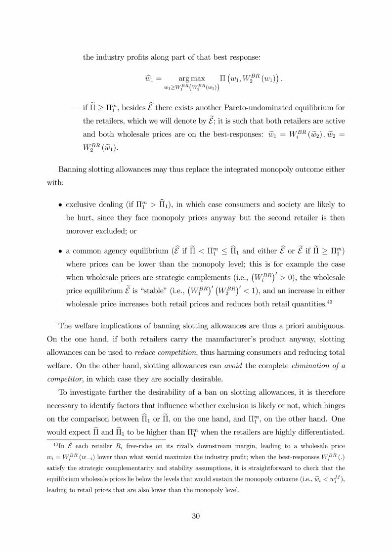
Banning slotting allowances may thus replace the integrated monopoly outcome either

with:

• exclusive dealing (if Πm1 > bΠ1), in which case consumers and society are likely tobe hurt, since they face monopoly prices anyway but the second retailer is then

morover excluded; or

• a common agency equilibrium (bE if eΠ < Πm1 ≤ bΠ1 and either bE or eE if eΠ ≥ Πm1 )

where prices can be lower than the monopoly level; this is for example the case

when wholesale prices are strategic complements (i.e.,¡WBRi

¢0> 0), the wholesale

price equilibrium eE is “stable” (i.e., ¡WBR1

¢0 ¡WBR2

¢0< 1), and an increase in either

wholesale price increases both retail prices and reduces both retail quantities.43

The welfare implications of banning slotting allowances are thus a priori ambiguous.

On the one hand, if both retailers carry the manufacturer’s product anyway, slotting

allowances can be used to reduce competition, thus harming consumers and reducing total

welfare. On the other hand, slotting allowances can avoid the complete elimination of a

competitor, in which case they are socially desirable.

To investigate further the desirability of a ban on slotting allowances, it is therefore

necessary to identify factors that influence whether exclusion is likely or not, which hinges

on the comparison between bΠ1 or eΠ, on the one hand, and Πm1 , on the other hand. One

would expect eΠ and bΠ1 to be higher than Πm1 when the retailers are highly differentiated.43In eE each retailer Ri free-rides on its rival’s downstream margin, leading to a wholesale price

wi =WBRi (w−i) lower than what would maximize the industry profit; when the best-responses WBR

i (.)

satisfy the strategic complementarity and stability assumptions, it is straightforward to check that the

equilibrium wholesale prices lie below the levels that would sustain the monopoly outcome (i.e., ewi < wMi ),leading to retail prices that are also lower than the monopoly level.

30

Indeed, if the retailers are selling on independent markets, then Πm = Πm1 + Πm2 and,

in addition, the pair Ri −M no longer has an incentive to free-ride on R−i’s sales (in

particular, Assumption A2 does not hold), so that the equilibrium profit is equal to the

monopoly profit: eΠ = Πm; therefore, bΠ ≥ eΠ > Πm1 , implying that both retailers can be

active even if slotting allowances are banned. If instead retailers are perfect substitutes,

Πm = Πm1 and bΠ1 < Πm; therefore, eΠ ≤ bΠ1 < Πm1 , implying that bE or eE cannot be theoutcome when slotting allowances are ruled out. Banning slotting allowances is therefore

more likely to induce exclusion when products are less differentiated.

A similar analysis can be made concerning the relative strengths of the retailers: the

inequality³eΠ ≤´ bΠ1 < Πm1 is more likely to hold when one retailer contributes much

more than the other to the industry profit (that is, Πm1 close to Πm); thus, symmetry may

render exclusion less likely.

In order to explore this question further, we now consider linear inverse demand func-

tions given by:

P1 (q1, q2) = 1−(1− α) q1 − σq2

1− σand P2 (q1, q2) = 1−

(1 + α) q2 − σq11− σ

,

where α,σ ∈ [0, 1[ and α + σ < 1, and normalize the production cost to c = 0. The

parameter α measures the asymmetry between the two retailers (retailers are equally

profitable when α = 0, while R1 becomes relatively larger than R2 as α increases) while σ

represents the degree of substitutability between the retailers (retailers face independent

demands when σ = 0, while they become closer substitutes as σ increases). The condition

α + σ < 1 ensures that both retailers are needed to maximize industry profits (i.e., that

the industry monopoly outcome assigns a positive quantity for R2).

The results obtained with this specification are illustrated in figures 1 and 2. Figure

1 shows the range of parameter values for which common agency equilibria exist when

slotting allowances are banned, for the cases of quantity (bold lines) and price (dashed

lines) competition.

31

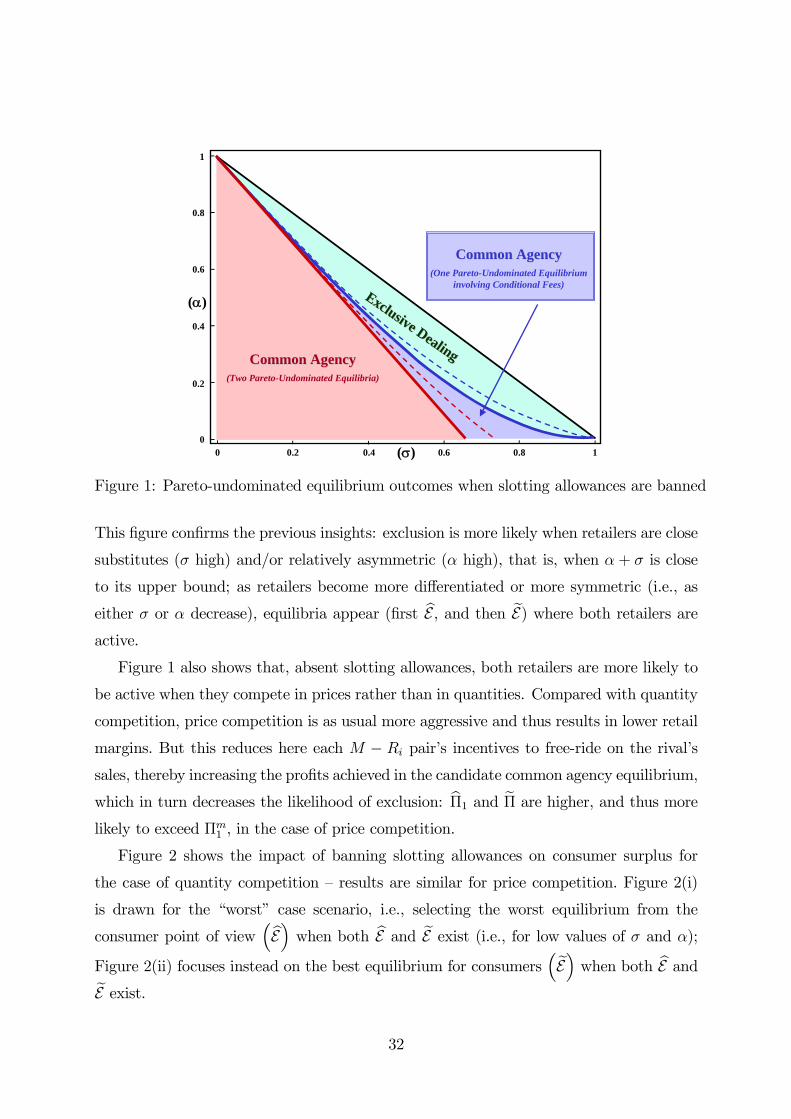
0 0.2 0.4 0.6 0.8 1

0

0.2

0.4

0.6

0.8

1

Exclusive

Exclusive DealingDealingCommon AgencyCommon Agency

(Two Pareto-Undominated Equilibria)

Common AgencyCommon Agency(One Pareto-Undominated Equilibrium

involving Conditional Fees)

(σ)0 0.2 0.4 0.6 0.8 1

(α)

0

0.2

0.4

0.6

0.8

1

Figure 1: Pareto-undominated equilibrium outcomes when slotting allowances are banned

This figure confirms the previous insights: exclusion is more likely when retailers are close

substitutes (σ high) and/or relatively asymmetric (α high), that is, when α + σ is close

to its upper bound; as retailers become more differentiated or more symmetric (i.e., as

either σ or α decrease), equilibria appear (first bE , and then eE) where both retailers areactive.

Figure 1 also shows that, absent slotting allowances, both retailers are more likely to

be active when they compete in prices rather than in quantities. Compared with quantity

competition, price competition is as usual more aggressive and thus results in lower retail

margins. But this reduces here each M − Ri pair’s incentives to free-ride on the rival’ssales, thereby increasing the profits achieved in the candidate common agency equilibrium,

which in turn decreases the likelihood of exclusion: bΠ1 and eΠ are higher, and thus morelikely to exceed Πm1 , in the case of price competition.

Figure 2 shows the impact of banning slotting allowances on consumer surplus for

the case of quantity competition — results are similar for price competition. Figure 2(i)

is drawn for the “worst” case scenario, i.e., selecting the worst equilibrium from the

consumer point of view³bE´ when both bE and eE exist (i.e., for low values of σ and α);

Figure 2(ii) focuses instead on the best equilibrium for consumers³eE´ when both bE andeE exist.

32

(σ)0 0.2 0.4 0.6 0.8 1

(α)

0

0.2

0.4

0.6

0.8

1

+0% / +10%

+10% / +20%

--6% / 6% / --2.5%

2.5%

--2.5% / 0%

2.5% / 0%

(i) bE selected(σ)0 0.2 0.4 0.6 0.8 1

(α)

0

0.2

0.4

0.6

0.8

1

+0%

/ +1

0%

--6% / 6% / --2.5%

2.5%

--2.5% / 0%

2.5% / 0%

+10%

/ +2

0%

+20%

/ +5

0%

+10% / +20%

> +50%

(ii) eE selectedFigure 2: Impact of banning slotting allowances on consumer surplus

Banning slotting allowances harms consumers (and society) when it leads to the exclu-

sive dealing. However, as already oberved, this is more likely to occur when retailers are

good substitutes and/or rather asymmetric (high values of σ and/or α), which is precisely

when the exclusion of the weaker retailer is socially less costly. As a result, the positive

effects of a ban on slotting allowances appear here likely to be larger than its negative

effects.44

8 Conclusion

This paper examines the role of upfront payments and conditional fixed fees in determining

market structure and retail prices. We first show that two-part tariffs cannot sustain the

industry monopoly outcome. This implies that the less efficient retailer may be excluded

in equilibrium. We also show that conditional fixed fees permit retailers to achieve higher

profits, by serving as a commitment to “opt out” in case prices become too low; this in

turn expands the scope for equilibria in which both retailers are active.44In the case of quantity competition, the results are the same when all negative fees are banned, rather

than only negative upfront ones. However, things change in that case when retailers compete in prices:

while the eE equilibrium is unaffected, the bE equilibrium becomes more competitive and thus exists less

often when negative conditional fees are banned as well. This extends the range of parameter values for

which banning negative payments has a negative impact but the qualitative analysis and the order of

magnitude of the effects remain the same.

33

Finally, combining conditional fixed fees with slotting allowances suffices to sustain

the industry monopoly outcome. This result is robust; in particular, it does not depend

on the type of retail competition (e.g. prices vs. quantities), nor on the amount of

retail differentiation or asymmetry. Even when they are close substitutes, the retailers

can commit to maintain monopoly prices (through adequate wholesale prices) by offering

conditional fixed fees equal to their anticipated profits, and then use slotting allowances to

recover from the manufacturer their contribution to the monopoly profits. In the absence

of any restriction on the tariffs, it is optimal for the retailers to combine in this way

slotting allowances and conditional fixed fees in order to sustain monopoly prices.

The welfare implications of banning slotting allowances are more ambiguous. Slotting

allowances may avoid the exclusion of some retailers but also eliminate any effective

competition between them. Relevant factors in assessing the implications in a given

market include such characteristics as the degree of substitutability and the symmetry

among the retailers. We find that slotting allowances are most likely to be detrimental to

welfare when retailers are not too close substitutes and rather symmetric.

As mentioned earlier, three-part tariffs are not the only way to achieve the monopoly

outcome. More general non-linear tariffs or even two-part tariffs combined with resale

price maintenance could also generate a similar outcome. However, these alternative

means still involve down payments (“slotting allowances”) by the manufacturer to the

retailers.

Our analysis also highlights the role of bargaining power. As mentioned earlier, much

of the literature on vertical contracting assumes that the bargaining power rests upstream.

Yet, in recent years the bargaining power has often shifted towards large retailers. Empir-

ical evidence indicates that the strong position of the retailers is positively correlated with

both the incidence and the magnitude of slotting allowances. Our analysis is in line with

this observation. Were bargaining power upstream, the industry monopoly outcome could

be achieved without slotting allowances; classic two-part tariffs, with positive fixed fees,

would suffice. Once retailers have some bargaining power, however, upfront payments by

the manufacturer are necessary to maintain monopoly prices.

In our analysis, where retailers can offer tariffs that are contingent on exclusivity, slot-

ting allowances always arise in the retailers’ preferred equilibrium, and in this equilibrium

both retailers are always active. In contrast, in Marx and Shaffer (2004) where contracts

are non-contingent, (negative) upfront payments only arise when retailers are asymmetric,

and whenever they arise they always lead to exclusion of a retailer.

34

An interesting extension would be to allow for less extreme bargaining power. While

it is easy to check that three-part tariffs keep implementing the monopoly outcome for

any degree of bargaining power (with upfront payments that increase with the retailers’

bargaining power), the equilibrium that would arise with only upfront or conditional

payments still needs to be explored.

35

References

[1] Allain, Marie-Laure and Claire Chambolle (2005), “Loss-Leaders Banning Laws as

Vertical Restraints.” Journal of Agricultural & Food Industrial Organization, 3, Ar-

ticle 5.

[2] Aghion, Philippe and Patrick Bolton (1987), “Contracts as a Barrier to Entry.”

American Economic Review, 77, 388-401.

[3] Battigalli, Pierpaolo, Chiara Fumagalli and Michele Polo (2006), “Buyer Power and

Quality Improvement.” IGIER Working Paper n◦310.

[4] Bernheim, Douglas and Michael Whinston (1985), “Common Marketing Agency as

a Device for Facilitating Collusion.” Rand Journal of Economics, 16, 269-281.

[5] Bernheim, Douglas and Michael Whinston (1998), “Exclusive Dealing.” Journal of

Political Economy, 106, 64-103.

[6] Bloom, Paul, Gregory Gundlach and Joseph Cannon (2000), “Slotting Allowances

and Fees: School of Thought and the Views of Practising Managers.” Journal of

Marketing, 64, 92-108.

[7] Comanor, William and Patrick Rey (2000), “Vertical Restraints and the Market

Power of Large Distributors.” Review of Industrial Organization, 17, 135-153.

[8] Competition Commission (2000), Supermarkets: A report on the supply of groceries

from multiple stores in the United Kingdom. Cm 4842, October 2000.

[9] de Fontenay, Catherine and Joshua Gans (2005a), “Bilateral Bargaining with Exter-

nalities.” Mimeo.

[10] de Fontenay, Catherine and Joshua Gans (2005b), “Vertical Integration in the Pres-

ence of Upstream Competition.” Rand Journal of Economics, 35(3), 544-572.

[11] Federal Trade Commission (2001), Report on the FTC Workshop on Slotting Al-

lowances and Other Marketing Practices in the Grocery Industry.

[12] Federal Trade Commission (2003), Slotting Allowances in the Retail Grocery Industry:

Selected Case Studies in Five Product Categories.

36

[13] Hart, Oliver and Jean Tirole (1990), “Vertical Integration and Market Foreclosure.”

Brookings Papers on Economic Activity: Microeconomics, 205-286.

[14] Kelly, Kenneth (1991), “Antitrust Analysis of Grocery Slotting Allowances: The

Procompetitive Case.”Journal of Public Policy and Marketing, 10, 187-198.

[15] Klein, Benjamin, and Joshua Wright (2006), “The Economics of Slotting Contracts.”

Mimeo.

[16] Inderst Roman (2005), “A Note on Buyer-Induced Exclusivity and the Role of Slot-

ting Fees.” Mimeo.

[17] Inderst, Roman and Christian Wey (2006), “Buyer Power and Supplier Incentives.”

forthcoming in European Economic Review..

[18] Mathewson, Frank and Ralph Winter (1987), “The Competitive Effects of Vertical

Agreements: Comments.” American Economic Review, 77, 1057-1062.

[19] Martimort, David and Lars Stole (2003), “Contractual Externalities and Common

Agency Equilibria.” Advances in Theoretical Economics, 3(1), Article 4.

[20] Marx, Leslie and Greg Shaffer (2004). “Upfront Payments and Exclusion in Down-

stream Markets.” Mimeo.

[21] McAfee, Preston and Marius Schwartz (1994), “Opportunism in Multilateral Vertical

Contracting: Nondiscrimination, Exclusivity and Uniformity.” American Economic

Review, 84, 210-230.

[22] O’Brien, Daniel and Greg Shaffer (1992), “Vertical Control with Bilateral Contracts.”

Rand Journal of Economics, 23, 299-308.

[23] Office of Fair Trading (2004), The supermarkets code of practice., OFT Report 697.

[24] Rasmusen, Eric, J. Mark Ramseyer, and John Wiley (1991), “Naked Exclusion.”

American Economic Review, 81, 1137-1145.

[25] Rey, Patrick and Jean Tirole (2006), “A Primer on Foreclosure.” Handbook of Indus-

trial Organization, Vol. 3, Mark Armstrong and Michael Porter Eds., North-Holland.

[26] Rey, Patrick and Thibaud Vergé (2002), “Resale Price Maintenance and Horizontal

Cartel.” CMPO Working Paper 02/048.

37

[27] Rey, Patrick and Thibaud Vergé (2004), “Bilateral Control with Vertical Contracts.”

Rand Journal of Economics, 35, 728-746.

[28] Segal, Ilya and Michael Whinston (2000), “Naked Exclusion: Comment.” American

Economic Review, 90, 296-311.

[29] Segal, Ilya and Michael Whinston (2003), “Robust Predictions for Bilateral Con-

tracting with Externalities.” Econometrica, 71(3), 757-791.

[30] Shaffer, Greg (1991), “Slotting Allowances and Resale Price Maintenance: A Com-

parison of Facilitating Practices.” Rand Journal of Economics, 22, 120-136.

[31] Shaffer, Greg (2005), “Slotting Allowances and Optimal Product Variety.” Advances

in Economic Analysis & Policy, 5(1), Article 3.

[32] Stole, Lars and Jeffrey Zwiebel (1996), “Intra-firm Bargaining and Non-binding Con-

tracts.” Review of Economic Studies, 63, 375-410.

38