Sloshing Tank Sbs Tutorial Cosmos
10
© COPYRIGHT 2008. All right reserved. No part of this documentation may be photocopied or reproduced in any form without prior written consent from COMSOL AB. COMSOL, COMSOL Multiphysics, COMSOL Reac- tion Engineering Lab, and FEMLAB are registered trademarks of COMSOL AB. Other product or brand names are trademarks or registered trademarks of their respective holders. Sloshi ng T ank SOLVED WITH COMSOL MULTIPHYSICS 3.5a ®
-
Upload
darklord338 -
Category
Documents
-
view
240 -
download
0
Transcript of Sloshing Tank Sbs Tutorial Cosmos
7212019 Sloshing Tank Sbs Tutorial Cosmos
httpslidepdfcomreaderfullsloshing-tank-sbs-tutorial-cosmos 110
copy COPYRIGHT 2008 All right reserved No part of this documentation may be photocopied or reproduced in
any form without prior written consent from COMSOL AB COMSOL COMSOL Multiphysics COMSOL Reac-
tion Engineering Lab and FEMLAB are registered trademarks of COMSOL AB Other product or brand names
are trademarks or registered trademarks of their respective holders
Sloshing TankSOLVED WITH COMSOL MULTIPHYSICS 35a
reg
7212019 Sloshing Tank Sbs Tutorial Cosmos
httpslidepdfcomreaderfullsloshing-tank-sbs-tutorial-cosmos 210
S L O S H I N G TA N K | 1
S l o s h i n g T ank
Introduction
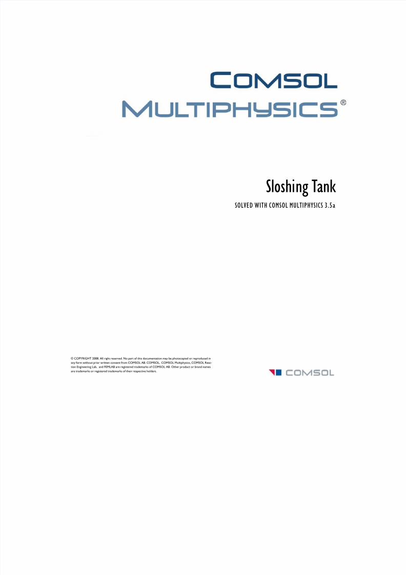
This 2D model demonstrates the ability of COMSOL Multiphysics to simulate
dynamic free surface flow with the help of a moving mesh The study models fluid
motion with the incompressible Navier-Stokes equations The fluid is initially at rest in
a rectangular tank The motion is driven by the gravity vector swinging back and forth
pointing up to 4 degrees away from the downward y direction at its extremes
Figure 1 Snapshots of the velocity field at t = 1 s t = 12 s t = 14 s and t = 16 s The
inclination of the gravity vector is indicated by the leaning of the tank
Because the surface of the fluid is free to move this model is a nonstandard
computational task The ALE (arbitrary Lagrangian-Eulerian) technique is however
well suited for addressing such problems Not only is it easy to set up using the Moving
Mesh (ALE) application mode in COMSOL Multiphysics but it also has the
advantage that it represents the free surface boundary with a domain boundary on the
moving mesh This allows for the accurate evaluation of surface properties such as
7212019 Sloshing Tank Sbs Tutorial Cosmos
httpslidepdfcomreaderfullsloshing-tank-sbs-tutorial-cosmos 310
S L O S H I N G TA N K | 2
curvature making surface tension analysis possible Note however that this example
model neglects surface tension effects
Model Definition
D O M A I N E Q U A T I O N S
This model describes the fluid dynamics with the incompressible Navier-Stokes
equations
where ρ is the density u = (u v) is the fluid velocity p is the pressure I is the unit
diagonal matrix η is the viscosity and F is the volume force In this example model
the material properties are for glycerol η = 149 Pamiddots and ρ = 127middot103 kgm3 The
gravity vector enters the force term as
where g = 981 ms2 and f = 1 Hz
With the help of the Moving Mesh (ALE) application mode you can solve these
equations on a freely moving deformed mesh which constitutes the fluid domain The
deformation of this mesh relative to the initial shape of the domain is computed using Winslow smoothing For more information please refer to ldquoThe Moving Mesh
Application Moderdquo on page 455 in the COMSOL Multiphysics Modeling Guide
COMSOL Multiphysics takes care of the transformation of the Navier-Stokes
equations to the formulation on the moving mesh
B O U N D A R Y C O N D I T I O N S F O R T H E F L U I D
There are two types of boundaries in the model domain Three solid walls that are
modeled with slip conditions and one free boundary (the top boundary) The slip
boundary condition for the Navier-Stokes equations is
where n = (n x n y)T is the boundary normal To enforce this boundary condition
select the Symmetry boundary type in the Incompressible Navier-Stokes application
ρtpart
partu ρu nablasdot u nabla pIndash η nablau nablau( )T +( )+( )sdotndash+ F=
nabla usdot 0=
F x ρ g φmax 2π ft( )sin( )sin=
F y ρndash g φmax 2π ft( )sin( )cos=
φmax 4π 180 frasl =
u nsdot 0=
7212019 Sloshing Tank Sbs Tutorial Cosmos
httpslidepdfcomreaderfullsloshing-tank-sbs-tutorial-cosmos 410
S L O S H I N G TA N K | 3
mode Because the normal vector depends on the degrees of freedom for the moving
mesh a constraint force would act not only on the fluid equations but also on the
moving mesh equations This effect would not be correct and one remedy is to usenon-ideal weak constraints Ideal weak constraints (the other type of weak constraints)
do not remove this effect of the constraint force For more information about weak
constraints see ldquoUsing Weak Constraintsrdquo on page 350 in the COMSOL Multiphysics
Modeling Guide The Incompressible Navier-Stokes application mode does not make
use of weak constraints by default so you need to activate the non-ideal weak
constraints
The following weak expression which you add to the model enforces the slip
boundary condition without a constraint force acting on the moving mesh equations
(1)
for some Lagrange multiplier variable λ Here λ and u denote test functions See the
step-by-step instructions later in this model documentation for details
The fluid is free to move on the top boundary The stress in the surroundingenvironment is neglected Therefore the stress continuity condition on the free
boundary reads
where p0 is the surrounding (constant) pressure and η the viscosity of the fluid
Without loss of generality p0 = 0 for this model
B O U N D A R Y C O N D I T I O N S F O R T H E M E S H
In order to follow the motion of the fluid with the moving mesh it is necessary to (at
least) couple the mesh motion to the fluid motion normal to the surface It turns out
that for this type of free surface motion it is important to not couple the mesh motion
to the fluid motion in the tangential direction If you would do so the mesh soon
becomes so deformed that the solution no longer converges The boundary condition
for the mesh equations on the free surface is therefore
where n is the boundary normal and ( xt yt)T the velocity of mesh (see ldquoMathematical
Description of the Mesh Movementrdquo on page 446 in the COMSOL Multiphysics
Modeling Guide ) In the Moving Mesh (ALE) application mode you specify this
boundary condition by selecting the tangent and normal coordinate system in the
λ u nsdot( ) λ u nsdot( )ndash
pIndash η unabla unabla( )T
+( )+( ) nsdot p0ndash n=
xt y t( )T
nsdot u nsdot=
7212019 Sloshing Tank Sbs Tutorial Cosmos
httpslidepdfcomreaderfullsloshing-tank-sbs-tutorial-cosmos 510
S L O S H I N G TA N K | 4
deformed mesh and by specifying a mesh velocity in the normal direction where you
enter the right-hand side expression from above as unx+vny The Moving Mesh
(ALE) application mode uses non-ideal weak constraints by default and for thisboundary condition it adds the weak expression
to ensure that there are no constraint forces acting on the fluid equations Here again
λ denotes some Lagrange multiplier variable (not the same as before) and λ x and y
denote test functions There is no need to modify this expression Choose
PhysicsgtEquation SystemgtBoundary Settings and select the free boundary (boundary 3)
to see how to enter this expression in COMSOL Multiphysics The expression implies
that there is a flux (or force) on the free boundary for the moving mesh coordinate
equations and respectively Furthermore to be able to
follow the fluid motion with the mesh motion the moving mesh must not be
constrained in the tangential direction on the side walls In the Moving Mesh (ALE)
application mode you specify this boundary condition by using the global coordinate
system and setting the mesh displacement to zero in the x direction At the bottom ofthe tank the mesh is fixed which you obtain in a similar way by setting the mesh
displacements to zero in both the x and y directions
Results
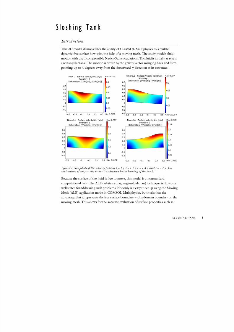
Figure 2 below and Figure 1 on page 1 show the tank at a few different points in time
The colors represent the velocity field Whereas you set up the model using a fixed tankand a swinging gravity vector deformation plots enable you to give the tank an
inclination at the postprocessing stage The inclination angle of the tank is exactly the
same as the angle of the gravity vector from its initial vertical position
λ xt yt( )T
undash( ) nsdot( ) λ x y( )T
nsdot( )ndash
xnabla nsdot λn x= ynabla nsdot λn y=
7212019 Sloshing Tank Sbs Tutorial Cosmos
httpslidepdfcomreaderfullsloshing-tank-sbs-tutorial-cosmos 610
S L O S H I N G TA N K | 5
Figure 2 Velocity field inside the tank at t = 6 s
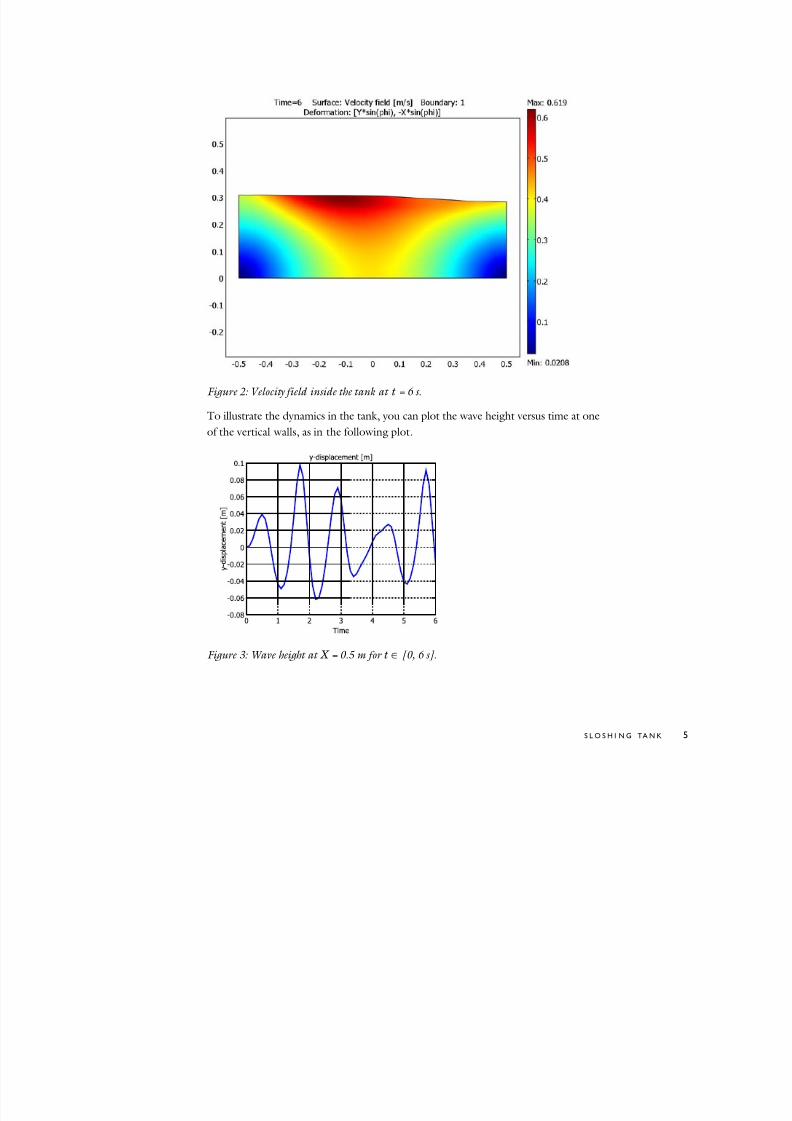
To illustrate the dynamics in the tank you can plot the wave height versus time at one
of the vertical walls as in the following plot
Figure 3 Wave height at X = 05 m for t isin [0 6 s]
7212019 Sloshing Tank Sbs Tutorial Cosmos
httpslidepdfcomreaderfullsloshing-tank-sbs-tutorial-cosmos 710
S L O S H I N G TA N K | 6
Model Library path COMSOL_MultiphysicsFluid_Dynamicssloshing_tank
Modeling Using the Graphical User Interface
1 Start COMSOL Multiphysics
2 In the Model Navigator click the Multiphysics button
3Select
2D from the
Space dimension list
4 Select COMSOL MultiphysicsgtDeformed MeshgtMoving Mesh (ALE)gtTransient analysis
and click Add
5 Click the Application Mode Properties button
6 Select Winslow from the Smoothing method list Click OK
7 Select COMSOL MultiphysicsgtFluid DynamicsgtIncompressible Navier-StokesgtTransient
analysis and click Add
8 Click OK
G E O M E T R Y M O D E L I N G
1 Shift-click the RectangleSquare button in the Draw toolbar
2 Specify the rectangle settings according to the table below
3 Click OK to close the Rectangle dialog box
4 Click the Zoom Extents button on the Main toolbar
PROPERTY EXPRESSION
Width 1
Height 03
Position Base Corner
Position X -05
Position Y 0
7212019 Sloshing Tank Sbs Tutorial Cosmos
httpslidepdfcomreaderfullsloshing-tank-sbs-tutorial-cosmos 810
S L O S H I N G TA N K | 7
O P T I O N S A N D S E T T I N G S
1 Open the Constants dialog box from the Options menu and enter the following
constants The descriptions are optional When done click OK
2 From the Options menu choose ExpressionsgtScalar Expressions
3 Enter the following scalar variables with names expressions and descriptions (the
descriptions are optional) when done click OK
P H Y S I C S S E T T I N G S
Properties
1 In the Incompressible Navier-Stokes application mode choose Properties from the
Physics menu
2 In the Application Mode Properties dialog box select On from the Weak constraints
list and Non-ideal from the Constraint type list then click OK
Subdomain Settings
Open the Subdomain Settings dialog box and apply the settings in the table below
NAME EXPRESSION DESCRIPTION
rho 1270[kgm^3] Glycerol density
nu 149[Pas] Glycerol viscosity
phi_max (4pi180)[rad] Maximum angle of inclination
freq 1[Hz] Frequency
g 981[ms^2] Acceleration due to gravity
NAME EXPRESSION DESCRIPTION
phi phi_maxsin(2pifreqt) Angle of inclination
grav_x gsin(phi) Gravity vector x component
grav_y -gcos(phi) Gravity vector y component
SETTINGS SUBDOMAIN 1
ρ rho
η nu
Fx grav_xrho
Fy grav_yrho
7212019 Sloshing Tank Sbs Tutorial Cosmos
httpslidepdfcomreaderfullsloshing-tank-sbs-tutorial-cosmos 910
S L O S H I N G TA N K | 8
Boundary Conditions
1 Open the Boundary Settings dialog box from the Physics menu and enter boundary
conditions according to the table below When done click OK
2 Go to the Multiphysics menu and select Moving Mesh (ALE) (ale)
3 In the Boundary Settings dialog box apply the following boundary conditions for the
mesh displacements (only tangential movements on the sides and a fixed mesh at the
bottom)
4 On Boundary 3 select Tangent and normal coord sys in deformed mesh in the
Coordinate system list Then click the Mesh velocity button and type unx+vny in
the vn edit field to specify the normal mesh velocity as u middotn
5 On the Weak Constr tab of the Boundary Settings dialog box clear the Use weak
constraints check box on Boundaries 1 2 and 4 The strong constraints that you
specified in the previous step are sufficient on these boundaries Leave the Use weak
constraints check box selected on Boundary 36 Click OK to close the dialog box
M E S H G E N E R A T I O N
Click the Initialize Mesh button on the Main toolbar to initialize the mesh
C O M P U T I N G T H E S O L U T I O N
1 Open the Solver Parameters dialog box from the Solve menu
2 Enter range(0016) in the Times edit field on the General page
3 Type 0001 in the Relative tolerance edit field This provides a 01 relative
tolerance which is one order of magnitude less than the default value
4 Click the Time Stepping tab
5 Select Exclude algebraic from the Error estimation strategy list This excludes the
pressure and the moving mesh variables from the error estimation The equations
SETTINGS BOUNDARIES 1 2 4 BOUNDARY 3
Boundary type Wall Open boundary
Boundary condition Slip Normal stress
f 0 0
SETTINGS BOUNDARIES 1 4 BOUNDARY 2
dx 0 0
dy 0
7212019 Sloshing Tank Sbs Tutorial Cosmos
httpslidepdfcomreaderfullsloshing-tank-sbs-tutorial-cosmos 1010
S L O S H I N G TA N K | 9
for those variables do not include time derivatives and become algebraic when
solving the equation system using the method of lines
6 Click OK
7 Click the Solve button on the Main toolbar
P O S T P R O C E S S I N G A N D V I S U A L I Z A T I O N
The default plot shows the x-component of the moving mesh deformation in the
spatial frame
1 To plot the velocity field of the glycerol instead go to the Surface tab in the Plot
Parameters dialog box and select Incompressible Navier-Stokes (ns)gtVelocity field
from the list of expressions
2 On the General page clear the Geometry edges check box Click Apply to see the plot
and use the Solution at time list on the General tab to browse through the output
times
You can visualize the tankrsquos inclination by clever use of the deformation plot feature
3 On the Deform page select the Deformed shape plot check box and set the Scale factor to 1 Enter Ysin(phi) in the X component edit field and -Xsin(phi) in the Y
component edit field on the Subdomain Data tab
4 Still on the Deform page click the Boundary Data tab Once again enter Ysin(phi)
in the X component edit field and -Xsin(phi) in the Y component edit field
5 On the Boundary tab select the Boundary plot check box Enter 1 in the Expression
edit field Select to use a Uniform color and pick a black color using the Color button
6 To get a more liquid-looking plot you may want to go to the Surface page and set
the Color table to GrayScale
7 Click Apply to see the plot
8 To see the waves in action go to the Animate page click Start Animation and then
click OK
To get a more comprehensive overview of the sloshing you can plot the
y-displacement from equilibrium in a point
1 Open the Domain Plot Parameters dialog box from the Postprocessing menu
2 On the Point tab select Point 4 from the Point selection list
3 Enter dy_ale in the Expression edit field then click OK to see the plot
7212019 Sloshing Tank Sbs Tutorial Cosmos
httpslidepdfcomreaderfullsloshing-tank-sbs-tutorial-cosmos 210
S L O S H I N G TA N K | 1
S l o s h i n g T ank
Introduction
This 2D model demonstrates the ability of COMSOL Multiphysics to simulate
dynamic free surface flow with the help of a moving mesh The study models fluid
motion with the incompressible Navier-Stokes equations The fluid is initially at rest in
a rectangular tank The motion is driven by the gravity vector swinging back and forth
pointing up to 4 degrees away from the downward y direction at its extremes
Figure 1 Snapshots of the velocity field at t = 1 s t = 12 s t = 14 s and t = 16 s The
inclination of the gravity vector is indicated by the leaning of the tank
Because the surface of the fluid is free to move this model is a nonstandard
computational task The ALE (arbitrary Lagrangian-Eulerian) technique is however
well suited for addressing such problems Not only is it easy to set up using the Moving
Mesh (ALE) application mode in COMSOL Multiphysics but it also has the
advantage that it represents the free surface boundary with a domain boundary on the
moving mesh This allows for the accurate evaluation of surface properties such as
7212019 Sloshing Tank Sbs Tutorial Cosmos
httpslidepdfcomreaderfullsloshing-tank-sbs-tutorial-cosmos 310
S L O S H I N G TA N K | 2
curvature making surface tension analysis possible Note however that this example
model neglects surface tension effects
Model Definition
D O M A I N E Q U A T I O N S
This model describes the fluid dynamics with the incompressible Navier-Stokes
equations
where ρ is the density u = (u v) is the fluid velocity p is the pressure I is the unit
diagonal matrix η is the viscosity and F is the volume force In this example model
the material properties are for glycerol η = 149 Pamiddots and ρ = 127middot103 kgm3 The
gravity vector enters the force term as
where g = 981 ms2 and f = 1 Hz
With the help of the Moving Mesh (ALE) application mode you can solve these
equations on a freely moving deformed mesh which constitutes the fluid domain The
deformation of this mesh relative to the initial shape of the domain is computed using Winslow smoothing For more information please refer to ldquoThe Moving Mesh
Application Moderdquo on page 455 in the COMSOL Multiphysics Modeling Guide
COMSOL Multiphysics takes care of the transformation of the Navier-Stokes
equations to the formulation on the moving mesh
B O U N D A R Y C O N D I T I O N S F O R T H E F L U I D
There are two types of boundaries in the model domain Three solid walls that are
modeled with slip conditions and one free boundary (the top boundary) The slip
boundary condition for the Navier-Stokes equations is
where n = (n x n y)T is the boundary normal To enforce this boundary condition
select the Symmetry boundary type in the Incompressible Navier-Stokes application
ρtpart
partu ρu nablasdot u nabla pIndash η nablau nablau( )T +( )+( )sdotndash+ F=
nabla usdot 0=
F x ρ g φmax 2π ft( )sin( )sin=
F y ρndash g φmax 2π ft( )sin( )cos=
φmax 4π 180 frasl =
u nsdot 0=
7212019 Sloshing Tank Sbs Tutorial Cosmos
httpslidepdfcomreaderfullsloshing-tank-sbs-tutorial-cosmos 410
S L O S H I N G TA N K | 3
mode Because the normal vector depends on the degrees of freedom for the moving
mesh a constraint force would act not only on the fluid equations but also on the
moving mesh equations This effect would not be correct and one remedy is to usenon-ideal weak constraints Ideal weak constraints (the other type of weak constraints)
do not remove this effect of the constraint force For more information about weak
constraints see ldquoUsing Weak Constraintsrdquo on page 350 in the COMSOL Multiphysics
Modeling Guide The Incompressible Navier-Stokes application mode does not make
use of weak constraints by default so you need to activate the non-ideal weak
constraints
The following weak expression which you add to the model enforces the slip
boundary condition without a constraint force acting on the moving mesh equations
(1)
for some Lagrange multiplier variable λ Here λ and u denote test functions See the
step-by-step instructions later in this model documentation for details
The fluid is free to move on the top boundary The stress in the surroundingenvironment is neglected Therefore the stress continuity condition on the free
boundary reads
where p0 is the surrounding (constant) pressure and η the viscosity of the fluid
Without loss of generality p0 = 0 for this model
B O U N D A R Y C O N D I T I O N S F O R T H E M E S H
In order to follow the motion of the fluid with the moving mesh it is necessary to (at
least) couple the mesh motion to the fluid motion normal to the surface It turns out
that for this type of free surface motion it is important to not couple the mesh motion
to the fluid motion in the tangential direction If you would do so the mesh soon
becomes so deformed that the solution no longer converges The boundary condition
for the mesh equations on the free surface is therefore
where n is the boundary normal and ( xt yt)T the velocity of mesh (see ldquoMathematical
Description of the Mesh Movementrdquo on page 446 in the COMSOL Multiphysics
Modeling Guide ) In the Moving Mesh (ALE) application mode you specify this
boundary condition by selecting the tangent and normal coordinate system in the
λ u nsdot( ) λ u nsdot( )ndash
pIndash η unabla unabla( )T
+( )+( ) nsdot p0ndash n=
xt y t( )T
nsdot u nsdot=
7212019 Sloshing Tank Sbs Tutorial Cosmos
httpslidepdfcomreaderfullsloshing-tank-sbs-tutorial-cosmos 510
S L O S H I N G TA N K | 4
deformed mesh and by specifying a mesh velocity in the normal direction where you
enter the right-hand side expression from above as unx+vny The Moving Mesh
(ALE) application mode uses non-ideal weak constraints by default and for thisboundary condition it adds the weak expression
to ensure that there are no constraint forces acting on the fluid equations Here again
λ denotes some Lagrange multiplier variable (not the same as before) and λ x and y
denote test functions There is no need to modify this expression Choose
PhysicsgtEquation SystemgtBoundary Settings and select the free boundary (boundary 3)
to see how to enter this expression in COMSOL Multiphysics The expression implies
that there is a flux (or force) on the free boundary for the moving mesh coordinate
equations and respectively Furthermore to be able to
follow the fluid motion with the mesh motion the moving mesh must not be
constrained in the tangential direction on the side walls In the Moving Mesh (ALE)
application mode you specify this boundary condition by using the global coordinate
system and setting the mesh displacement to zero in the x direction At the bottom ofthe tank the mesh is fixed which you obtain in a similar way by setting the mesh
displacements to zero in both the x and y directions
Results
Figure 2 below and Figure 1 on page 1 show the tank at a few different points in time
The colors represent the velocity field Whereas you set up the model using a fixed tankand a swinging gravity vector deformation plots enable you to give the tank an
inclination at the postprocessing stage The inclination angle of the tank is exactly the
same as the angle of the gravity vector from its initial vertical position
λ xt yt( )T
undash( ) nsdot( ) λ x y( )T
nsdot( )ndash
xnabla nsdot λn x= ynabla nsdot λn y=
7212019 Sloshing Tank Sbs Tutorial Cosmos
httpslidepdfcomreaderfullsloshing-tank-sbs-tutorial-cosmos 610
S L O S H I N G TA N K | 5
Figure 2 Velocity field inside the tank at t = 6 s
To illustrate the dynamics in the tank you can plot the wave height versus time at one
of the vertical walls as in the following plot
Figure 3 Wave height at X = 05 m for t isin [0 6 s]
7212019 Sloshing Tank Sbs Tutorial Cosmos
httpslidepdfcomreaderfullsloshing-tank-sbs-tutorial-cosmos 710
S L O S H I N G TA N K | 6
Model Library path COMSOL_MultiphysicsFluid_Dynamicssloshing_tank
Modeling Using the Graphical User Interface
1 Start COMSOL Multiphysics
2 In the Model Navigator click the Multiphysics button
3Select
2D from the
Space dimension list
4 Select COMSOL MultiphysicsgtDeformed MeshgtMoving Mesh (ALE)gtTransient analysis
and click Add
5 Click the Application Mode Properties button
6 Select Winslow from the Smoothing method list Click OK
7 Select COMSOL MultiphysicsgtFluid DynamicsgtIncompressible Navier-StokesgtTransient
analysis and click Add
8 Click OK
G E O M E T R Y M O D E L I N G
1 Shift-click the RectangleSquare button in the Draw toolbar
2 Specify the rectangle settings according to the table below
3 Click OK to close the Rectangle dialog box
4 Click the Zoom Extents button on the Main toolbar
PROPERTY EXPRESSION
Width 1
Height 03
Position Base Corner
Position X -05
Position Y 0
7212019 Sloshing Tank Sbs Tutorial Cosmos
httpslidepdfcomreaderfullsloshing-tank-sbs-tutorial-cosmos 810
S L O S H I N G TA N K | 7
O P T I O N S A N D S E T T I N G S
1 Open the Constants dialog box from the Options menu and enter the following
constants The descriptions are optional When done click OK
2 From the Options menu choose ExpressionsgtScalar Expressions
3 Enter the following scalar variables with names expressions and descriptions (the
descriptions are optional) when done click OK
P H Y S I C S S E T T I N G S
Properties
1 In the Incompressible Navier-Stokes application mode choose Properties from the
Physics menu
2 In the Application Mode Properties dialog box select On from the Weak constraints
list and Non-ideal from the Constraint type list then click OK
Subdomain Settings
Open the Subdomain Settings dialog box and apply the settings in the table below
NAME EXPRESSION DESCRIPTION
rho 1270[kgm^3] Glycerol density
nu 149[Pas] Glycerol viscosity
phi_max (4pi180)[rad] Maximum angle of inclination
freq 1[Hz] Frequency
g 981[ms^2] Acceleration due to gravity
NAME EXPRESSION DESCRIPTION
phi phi_maxsin(2pifreqt) Angle of inclination
grav_x gsin(phi) Gravity vector x component
grav_y -gcos(phi) Gravity vector y component
SETTINGS SUBDOMAIN 1
ρ rho
η nu
Fx grav_xrho
Fy grav_yrho
7212019 Sloshing Tank Sbs Tutorial Cosmos
httpslidepdfcomreaderfullsloshing-tank-sbs-tutorial-cosmos 910
S L O S H I N G TA N K | 8
Boundary Conditions
1 Open the Boundary Settings dialog box from the Physics menu and enter boundary
conditions according to the table below When done click OK
2 Go to the Multiphysics menu and select Moving Mesh (ALE) (ale)
3 In the Boundary Settings dialog box apply the following boundary conditions for the
mesh displacements (only tangential movements on the sides and a fixed mesh at the
bottom)
4 On Boundary 3 select Tangent and normal coord sys in deformed mesh in the
Coordinate system list Then click the Mesh velocity button and type unx+vny in
the vn edit field to specify the normal mesh velocity as u middotn
5 On the Weak Constr tab of the Boundary Settings dialog box clear the Use weak
constraints check box on Boundaries 1 2 and 4 The strong constraints that you
specified in the previous step are sufficient on these boundaries Leave the Use weak
constraints check box selected on Boundary 36 Click OK to close the dialog box
M E S H G E N E R A T I O N
Click the Initialize Mesh button on the Main toolbar to initialize the mesh
C O M P U T I N G T H E S O L U T I O N
1 Open the Solver Parameters dialog box from the Solve menu
2 Enter range(0016) in the Times edit field on the General page
3 Type 0001 in the Relative tolerance edit field This provides a 01 relative
tolerance which is one order of magnitude less than the default value
4 Click the Time Stepping tab
5 Select Exclude algebraic from the Error estimation strategy list This excludes the
pressure and the moving mesh variables from the error estimation The equations
SETTINGS BOUNDARIES 1 2 4 BOUNDARY 3
Boundary type Wall Open boundary
Boundary condition Slip Normal stress
f 0 0
SETTINGS BOUNDARIES 1 4 BOUNDARY 2
dx 0 0
dy 0
7212019 Sloshing Tank Sbs Tutorial Cosmos
httpslidepdfcomreaderfullsloshing-tank-sbs-tutorial-cosmos 1010
S L O S H I N G TA N K | 9
for those variables do not include time derivatives and become algebraic when
solving the equation system using the method of lines
6 Click OK
7 Click the Solve button on the Main toolbar
P O S T P R O C E S S I N G A N D V I S U A L I Z A T I O N
The default plot shows the x-component of the moving mesh deformation in the
spatial frame
1 To plot the velocity field of the glycerol instead go to the Surface tab in the Plot
Parameters dialog box and select Incompressible Navier-Stokes (ns)gtVelocity field
from the list of expressions
2 On the General page clear the Geometry edges check box Click Apply to see the plot
and use the Solution at time list on the General tab to browse through the output
times
You can visualize the tankrsquos inclination by clever use of the deformation plot feature
3 On the Deform page select the Deformed shape plot check box and set the Scale factor to 1 Enter Ysin(phi) in the X component edit field and -Xsin(phi) in the Y
component edit field on the Subdomain Data tab
4 Still on the Deform page click the Boundary Data tab Once again enter Ysin(phi)
in the X component edit field and -Xsin(phi) in the Y component edit field
5 On the Boundary tab select the Boundary plot check box Enter 1 in the Expression
edit field Select to use a Uniform color and pick a black color using the Color button
6 To get a more liquid-looking plot you may want to go to the Surface page and set
the Color table to GrayScale
7 Click Apply to see the plot
8 To see the waves in action go to the Animate page click Start Animation and then
click OK
To get a more comprehensive overview of the sloshing you can plot the
y-displacement from equilibrium in a point
1 Open the Domain Plot Parameters dialog box from the Postprocessing menu
2 On the Point tab select Point 4 from the Point selection list
3 Enter dy_ale in the Expression edit field then click OK to see the plot

7212019 Sloshing Tank Sbs Tutorial Cosmos
httpslidepdfcomreaderfullsloshing-tank-sbs-tutorial-cosmos 510
S L O S H I N G TA N K | 4
deformed mesh and by specifying a mesh velocity in the normal direction where you
enter the right-hand side expression from above as unx+vny The Moving Mesh
(ALE) application mode uses non-ideal weak constraints by default and for thisboundary condition it adds the weak expression
to ensure that there are no constraint forces acting on the fluid equations Here again
λ denotes some Lagrange multiplier variable (not the same as before) and λ x and y
denote test functions There is no need to modify this expression Choose
PhysicsgtEquation SystemgtBoundary Settings and select the free boundary (boundary 3)
to see how to enter this expression in COMSOL Multiphysics The expression implies
that there is a flux (or force) on the free boundary for the moving mesh coordinate
equations and respectively Furthermore to be able to
follow the fluid motion with the mesh motion the moving mesh must not be
constrained in the tangential direction on the side walls In the Moving Mesh (ALE)
application mode you specify this boundary condition by using the global coordinate
system and setting the mesh displacement to zero in the x direction At the bottom ofthe tank the mesh is fixed which you obtain in a similar way by setting the mesh
displacements to zero in both the x and y directions
Results
Figure 2 below and Figure 1 on page 1 show the tank at a few different points in time
The colors represent the velocity field Whereas you set up the model using a fixed tankand a swinging gravity vector deformation plots enable you to give the tank an
inclination at the postprocessing stage The inclination angle of the tank is exactly the
same as the angle of the gravity vector from its initial vertical position
λ xt yt( )T
undash( ) nsdot( ) λ x y( )T
nsdot( )ndash
xnabla nsdot λn x= ynabla nsdot λn y=
7212019 Sloshing Tank Sbs Tutorial Cosmos
httpslidepdfcomreaderfullsloshing-tank-sbs-tutorial-cosmos 610
S L O S H I N G TA N K | 5
Figure 2 Velocity field inside the tank at t = 6 s
To illustrate the dynamics in the tank you can plot the wave height versus time at one
of the vertical walls as in the following plot
Figure 3 Wave height at X = 05 m for t isin [0 6 s]
7212019 Sloshing Tank Sbs Tutorial Cosmos
httpslidepdfcomreaderfullsloshing-tank-sbs-tutorial-cosmos 710
S L O S H I N G TA N K | 6
Model Library path COMSOL_MultiphysicsFluid_Dynamicssloshing_tank
Modeling Using the Graphical User Interface
1 Start COMSOL Multiphysics
2 In the Model Navigator click the Multiphysics button
3Select
2D from the
Space dimension list
4 Select COMSOL MultiphysicsgtDeformed MeshgtMoving Mesh (ALE)gtTransient analysis
and click Add
5 Click the Application Mode Properties button
6 Select Winslow from the Smoothing method list Click OK
7 Select COMSOL MultiphysicsgtFluid DynamicsgtIncompressible Navier-StokesgtTransient
analysis and click Add
8 Click OK
G E O M E T R Y M O D E L I N G
1 Shift-click the RectangleSquare button in the Draw toolbar
2 Specify the rectangle settings according to the table below
3 Click OK to close the Rectangle dialog box
4 Click the Zoom Extents button on the Main toolbar
PROPERTY EXPRESSION
Width 1
Height 03
Position Base Corner
Position X -05
Position Y 0
7212019 Sloshing Tank Sbs Tutorial Cosmos
httpslidepdfcomreaderfullsloshing-tank-sbs-tutorial-cosmos 810
S L O S H I N G TA N K | 7
O P T I O N S A N D S E T T I N G S
1 Open the Constants dialog box from the Options menu and enter the following
constants The descriptions are optional When done click OK
2 From the Options menu choose ExpressionsgtScalar Expressions
3 Enter the following scalar variables with names expressions and descriptions (the
descriptions are optional) when done click OK
P H Y S I C S S E T T I N G S
Properties
1 In the Incompressible Navier-Stokes application mode choose Properties from the
Physics menu
2 In the Application Mode Properties dialog box select On from the Weak constraints
list and Non-ideal from the Constraint type list then click OK
Subdomain Settings
Open the Subdomain Settings dialog box and apply the settings in the table below
NAME EXPRESSION DESCRIPTION
rho 1270[kgm^3] Glycerol density
nu 149[Pas] Glycerol viscosity
phi_max (4pi180)[rad] Maximum angle of inclination
freq 1[Hz] Frequency
g 981[ms^2] Acceleration due to gravity
NAME EXPRESSION DESCRIPTION
phi phi_maxsin(2pifreqt) Angle of inclination
grav_x gsin(phi) Gravity vector x component
grav_y -gcos(phi) Gravity vector y component
SETTINGS SUBDOMAIN 1
ρ rho
η nu
Fx grav_xrho
Fy grav_yrho
7212019 Sloshing Tank Sbs Tutorial Cosmos
httpslidepdfcomreaderfullsloshing-tank-sbs-tutorial-cosmos 910
S L O S H I N G TA N K | 8
Boundary Conditions
1 Open the Boundary Settings dialog box from the Physics menu and enter boundary
conditions according to the table below When done click OK
2 Go to the Multiphysics menu and select Moving Mesh (ALE) (ale)
3 In the Boundary Settings dialog box apply the following boundary conditions for the
mesh displacements (only tangential movements on the sides and a fixed mesh at the
bottom)
4 On Boundary 3 select Tangent and normal coord sys in deformed mesh in the
Coordinate system list Then click the Mesh velocity button and type unx+vny in
the vn edit field to specify the normal mesh velocity as u middotn
5 On the Weak Constr tab of the Boundary Settings dialog box clear the Use weak
constraints check box on Boundaries 1 2 and 4 The strong constraints that you
specified in the previous step are sufficient on these boundaries Leave the Use weak
constraints check box selected on Boundary 36 Click OK to close the dialog box
M E S H G E N E R A T I O N
Click the Initialize Mesh button on the Main toolbar to initialize the mesh
C O M P U T I N G T H E S O L U T I O N
1 Open the Solver Parameters dialog box from the Solve menu
2 Enter range(0016) in the Times edit field on the General page
3 Type 0001 in the Relative tolerance edit field This provides a 01 relative
tolerance which is one order of magnitude less than the default value
4 Click the Time Stepping tab
5 Select Exclude algebraic from the Error estimation strategy list This excludes the
pressure and the moving mesh variables from the error estimation The equations
SETTINGS BOUNDARIES 1 2 4 BOUNDARY 3
Boundary type Wall Open boundary
Boundary condition Slip Normal stress
f 0 0
SETTINGS BOUNDARIES 1 4 BOUNDARY 2
dx 0 0
dy 0
7212019 Sloshing Tank Sbs Tutorial Cosmos
httpslidepdfcomreaderfullsloshing-tank-sbs-tutorial-cosmos 1010
S L O S H I N G TA N K | 9
for those variables do not include time derivatives and become algebraic when
solving the equation system using the method of lines
6 Click OK
7 Click the Solve button on the Main toolbar
P O S T P R O C E S S I N G A N D V I S U A L I Z A T I O N
The default plot shows the x-component of the moving mesh deformation in the
spatial frame
1 To plot the velocity field of the glycerol instead go to the Surface tab in the Plot
Parameters dialog box and select Incompressible Navier-Stokes (ns)gtVelocity field
from the list of expressions
2 On the General page clear the Geometry edges check box Click Apply to see the plot
and use the Solution at time list on the General tab to browse through the output
times
You can visualize the tankrsquos inclination by clever use of the deformation plot feature
3 On the Deform page select the Deformed shape plot check box and set the Scale factor to 1 Enter Ysin(phi) in the X component edit field and -Xsin(phi) in the Y
component edit field on the Subdomain Data tab
4 Still on the Deform page click the Boundary Data tab Once again enter Ysin(phi)
in the X component edit field and -Xsin(phi) in the Y component edit field
5 On the Boundary tab select the Boundary plot check box Enter 1 in the Expression
edit field Select to use a Uniform color and pick a black color using the Color button
6 To get a more liquid-looking plot you may want to go to the Surface page and set
the Color table to GrayScale
7 Click Apply to see the plot
8 To see the waves in action go to the Animate page click Start Animation and then
click OK
To get a more comprehensive overview of the sloshing you can plot the
y-displacement from equilibrium in a point
1 Open the Domain Plot Parameters dialog box from the Postprocessing menu
2 On the Point tab select Point 4 from the Point selection list
3 Enter dy_ale in the Expression edit field then click OK to see the plot
7212019 Sloshing Tank Sbs Tutorial Cosmos
httpslidepdfcomreaderfullsloshing-tank-sbs-tutorial-cosmos 610
S L O S H I N G TA N K | 5
Figure 2 Velocity field inside the tank at t = 6 s
To illustrate the dynamics in the tank you can plot the wave height versus time at one
of the vertical walls as in the following plot
Figure 3 Wave height at X = 05 m for t isin [0 6 s]
7212019 Sloshing Tank Sbs Tutorial Cosmos
httpslidepdfcomreaderfullsloshing-tank-sbs-tutorial-cosmos 710
S L O S H I N G TA N K | 6
Model Library path COMSOL_MultiphysicsFluid_Dynamicssloshing_tank
Modeling Using the Graphical User Interface
1 Start COMSOL Multiphysics
2 In the Model Navigator click the Multiphysics button
3Select
2D from the
Space dimension list
4 Select COMSOL MultiphysicsgtDeformed MeshgtMoving Mesh (ALE)gtTransient analysis
and click Add
5 Click the Application Mode Properties button
6 Select Winslow from the Smoothing method list Click OK
7 Select COMSOL MultiphysicsgtFluid DynamicsgtIncompressible Navier-StokesgtTransient
analysis and click Add
8 Click OK
G E O M E T R Y M O D E L I N G
1 Shift-click the RectangleSquare button in the Draw toolbar
2 Specify the rectangle settings according to the table below
3 Click OK to close the Rectangle dialog box
4 Click the Zoom Extents button on the Main toolbar
PROPERTY EXPRESSION
Width 1
Height 03
Position Base Corner
Position X -05
Position Y 0
7212019 Sloshing Tank Sbs Tutorial Cosmos
httpslidepdfcomreaderfullsloshing-tank-sbs-tutorial-cosmos 810
S L O S H I N G TA N K | 7
O P T I O N S A N D S E T T I N G S
1 Open the Constants dialog box from the Options menu and enter the following
constants The descriptions are optional When done click OK
2 From the Options menu choose ExpressionsgtScalar Expressions
3 Enter the following scalar variables with names expressions and descriptions (the
descriptions are optional) when done click OK
P H Y S I C S S E T T I N G S
Properties
1 In the Incompressible Navier-Stokes application mode choose Properties from the
Physics menu
2 In the Application Mode Properties dialog box select On from the Weak constraints
list and Non-ideal from the Constraint type list then click OK
Subdomain Settings
Open the Subdomain Settings dialog box and apply the settings in the table below
NAME EXPRESSION DESCRIPTION
rho 1270[kgm^3] Glycerol density
nu 149[Pas] Glycerol viscosity
phi_max (4pi180)[rad] Maximum angle of inclination
freq 1[Hz] Frequency
g 981[ms^2] Acceleration due to gravity
NAME EXPRESSION DESCRIPTION
phi phi_maxsin(2pifreqt) Angle of inclination
grav_x gsin(phi) Gravity vector x component
grav_y -gcos(phi) Gravity vector y component
SETTINGS SUBDOMAIN 1
ρ rho
η nu
Fx grav_xrho
Fy grav_yrho
7212019 Sloshing Tank Sbs Tutorial Cosmos
httpslidepdfcomreaderfullsloshing-tank-sbs-tutorial-cosmos 910
S L O S H I N G TA N K | 8
Boundary Conditions
1 Open the Boundary Settings dialog box from the Physics menu and enter boundary
conditions according to the table below When done click OK
2 Go to the Multiphysics menu and select Moving Mesh (ALE) (ale)
3 In the Boundary Settings dialog box apply the following boundary conditions for the
mesh displacements (only tangential movements on the sides and a fixed mesh at the
bottom)
4 On Boundary 3 select Tangent and normal coord sys in deformed mesh in the
Coordinate system list Then click the Mesh velocity button and type unx+vny in
the vn edit field to specify the normal mesh velocity as u middotn
5 On the Weak Constr tab of the Boundary Settings dialog box clear the Use weak
constraints check box on Boundaries 1 2 and 4 The strong constraints that you
specified in the previous step are sufficient on these boundaries Leave the Use weak
constraints check box selected on Boundary 36 Click OK to close the dialog box
M E S H G E N E R A T I O N
Click the Initialize Mesh button on the Main toolbar to initialize the mesh
C O M P U T I N G T H E S O L U T I O N
1 Open the Solver Parameters dialog box from the Solve menu
2 Enter range(0016) in the Times edit field on the General page
3 Type 0001 in the Relative tolerance edit field This provides a 01 relative
tolerance which is one order of magnitude less than the default value
4 Click the Time Stepping tab
5 Select Exclude algebraic from the Error estimation strategy list This excludes the
pressure and the moving mesh variables from the error estimation The equations
SETTINGS BOUNDARIES 1 2 4 BOUNDARY 3
Boundary type Wall Open boundary
Boundary condition Slip Normal stress
f 0 0
SETTINGS BOUNDARIES 1 4 BOUNDARY 2
dx 0 0
dy 0
7212019 Sloshing Tank Sbs Tutorial Cosmos
httpslidepdfcomreaderfullsloshing-tank-sbs-tutorial-cosmos 1010
S L O S H I N G TA N K | 9
for those variables do not include time derivatives and become algebraic when
solving the equation system using the method of lines
6 Click OK
7 Click the Solve button on the Main toolbar
P O S T P R O C E S S I N G A N D V I S U A L I Z A T I O N
The default plot shows the x-component of the moving mesh deformation in the
spatial frame
1 To plot the velocity field of the glycerol instead go to the Surface tab in the Plot
Parameters dialog box and select Incompressible Navier-Stokes (ns)gtVelocity field
from the list of expressions
2 On the General page clear the Geometry edges check box Click Apply to see the plot
and use the Solution at time list on the General tab to browse through the output
times
You can visualize the tankrsquos inclination by clever use of the deformation plot feature
3 On the Deform page select the Deformed shape plot check box and set the Scale factor to 1 Enter Ysin(phi) in the X component edit field and -Xsin(phi) in the Y
component edit field on the Subdomain Data tab
4 Still on the Deform page click the Boundary Data tab Once again enter Ysin(phi)
in the X component edit field and -Xsin(phi) in the Y component edit field
5 On the Boundary tab select the Boundary plot check box Enter 1 in the Expression
edit field Select to use a Uniform color and pick a black color using the Color button
6 To get a more liquid-looking plot you may want to go to the Surface page and set
the Color table to GrayScale
7 Click Apply to see the plot
8 To see the waves in action go to the Animate page click Start Animation and then
click OK
To get a more comprehensive overview of the sloshing you can plot the
y-displacement from equilibrium in a point
1 Open the Domain Plot Parameters dialog box from the Postprocessing menu
2 On the Point tab select Point 4 from the Point selection list
3 Enter dy_ale in the Expression edit field then click OK to see the plot

7212019 Sloshing Tank Sbs Tutorial Cosmos
httpslidepdfcomreaderfullsloshing-tank-sbs-tutorial-cosmos 710
S L O S H I N G TA N K | 6
Model Library path COMSOL_MultiphysicsFluid_Dynamicssloshing_tank
Modeling Using the Graphical User Interface
1 Start COMSOL Multiphysics
2 In the Model Navigator click the Multiphysics button
3Select
2D from the
Space dimension list
4 Select COMSOL MultiphysicsgtDeformed MeshgtMoving Mesh (ALE)gtTransient analysis
and click Add
5 Click the Application Mode Properties button
6 Select Winslow from the Smoothing method list Click OK
7 Select COMSOL MultiphysicsgtFluid DynamicsgtIncompressible Navier-StokesgtTransient
analysis and click Add
8 Click OK
G E O M E T R Y M O D E L I N G
1 Shift-click the RectangleSquare button in the Draw toolbar
2 Specify the rectangle settings according to the table below
3 Click OK to close the Rectangle dialog box
4 Click the Zoom Extents button on the Main toolbar
PROPERTY EXPRESSION
Width 1
Height 03
Position Base Corner
Position X -05
Position Y 0
7212019 Sloshing Tank Sbs Tutorial Cosmos
httpslidepdfcomreaderfullsloshing-tank-sbs-tutorial-cosmos 810
S L O S H I N G TA N K | 7
O P T I O N S A N D S E T T I N G S
1 Open the Constants dialog box from the Options menu and enter the following
constants The descriptions are optional When done click OK
2 From the Options menu choose ExpressionsgtScalar Expressions
3 Enter the following scalar variables with names expressions and descriptions (the
descriptions are optional) when done click OK
P H Y S I C S S E T T I N G S
Properties
1 In the Incompressible Navier-Stokes application mode choose Properties from the
Physics menu
2 In the Application Mode Properties dialog box select On from the Weak constraints
list and Non-ideal from the Constraint type list then click OK
Subdomain Settings
Open the Subdomain Settings dialog box and apply the settings in the table below
NAME EXPRESSION DESCRIPTION
rho 1270[kgm^3] Glycerol density
nu 149[Pas] Glycerol viscosity
phi_max (4pi180)[rad] Maximum angle of inclination
freq 1[Hz] Frequency
g 981[ms^2] Acceleration due to gravity
NAME EXPRESSION DESCRIPTION
phi phi_maxsin(2pifreqt) Angle of inclination
grav_x gsin(phi) Gravity vector x component
grav_y -gcos(phi) Gravity vector y component
SETTINGS SUBDOMAIN 1
ρ rho
η nu
Fx grav_xrho
Fy grav_yrho
7212019 Sloshing Tank Sbs Tutorial Cosmos
httpslidepdfcomreaderfullsloshing-tank-sbs-tutorial-cosmos 910
S L O S H I N G TA N K | 8
Boundary Conditions
1 Open the Boundary Settings dialog box from the Physics menu and enter boundary
conditions according to the table below When done click OK
2 Go to the Multiphysics menu and select Moving Mesh (ALE) (ale)
3 In the Boundary Settings dialog box apply the following boundary conditions for the
mesh displacements (only tangential movements on the sides and a fixed mesh at the
bottom)
4 On Boundary 3 select Tangent and normal coord sys in deformed mesh in the
Coordinate system list Then click the Mesh velocity button and type unx+vny in
the vn edit field to specify the normal mesh velocity as u middotn
5 On the Weak Constr tab of the Boundary Settings dialog box clear the Use weak
constraints check box on Boundaries 1 2 and 4 The strong constraints that you
specified in the previous step are sufficient on these boundaries Leave the Use weak
constraints check box selected on Boundary 36 Click OK to close the dialog box
M E S H G E N E R A T I O N
Click the Initialize Mesh button on the Main toolbar to initialize the mesh
C O M P U T I N G T H E S O L U T I O N
1 Open the Solver Parameters dialog box from the Solve menu
2 Enter range(0016) in the Times edit field on the General page
3 Type 0001 in the Relative tolerance edit field This provides a 01 relative
tolerance which is one order of magnitude less than the default value
4 Click the Time Stepping tab
5 Select Exclude algebraic from the Error estimation strategy list This excludes the
pressure and the moving mesh variables from the error estimation The equations
SETTINGS BOUNDARIES 1 2 4 BOUNDARY 3
Boundary type Wall Open boundary
Boundary condition Slip Normal stress
f 0 0
SETTINGS BOUNDARIES 1 4 BOUNDARY 2
dx 0 0
dy 0
7212019 Sloshing Tank Sbs Tutorial Cosmos
httpslidepdfcomreaderfullsloshing-tank-sbs-tutorial-cosmos 1010
S L O S H I N G TA N K | 9
for those variables do not include time derivatives and become algebraic when
solving the equation system using the method of lines
6 Click OK
7 Click the Solve button on the Main toolbar
P O S T P R O C E S S I N G A N D V I S U A L I Z A T I O N
The default plot shows the x-component of the moving mesh deformation in the
spatial frame
1 To plot the velocity field of the glycerol instead go to the Surface tab in the Plot
Parameters dialog box and select Incompressible Navier-Stokes (ns)gtVelocity field
from the list of expressions
2 On the General page clear the Geometry edges check box Click Apply to see the plot
and use the Solution at time list on the General tab to browse through the output
times
You can visualize the tankrsquos inclination by clever use of the deformation plot feature
3 On the Deform page select the Deformed shape plot check box and set the Scale factor to 1 Enter Ysin(phi) in the X component edit field and -Xsin(phi) in the Y
component edit field on the Subdomain Data tab
4 Still on the Deform page click the Boundary Data tab Once again enter Ysin(phi)
in the X component edit field and -Xsin(phi) in the Y component edit field
5 On the Boundary tab select the Boundary plot check box Enter 1 in the Expression
edit field Select to use a Uniform color and pick a black color using the Color button
6 To get a more liquid-looking plot you may want to go to the Surface page and set
the Color table to GrayScale
7 Click Apply to see the plot
8 To see the waves in action go to the Animate page click Start Animation and then
click OK
To get a more comprehensive overview of the sloshing you can plot the
y-displacement from equilibrium in a point
1 Open the Domain Plot Parameters dialog box from the Postprocessing menu
2 On the Point tab select Point 4 from the Point selection list
3 Enter dy_ale in the Expression edit field then click OK to see the plot
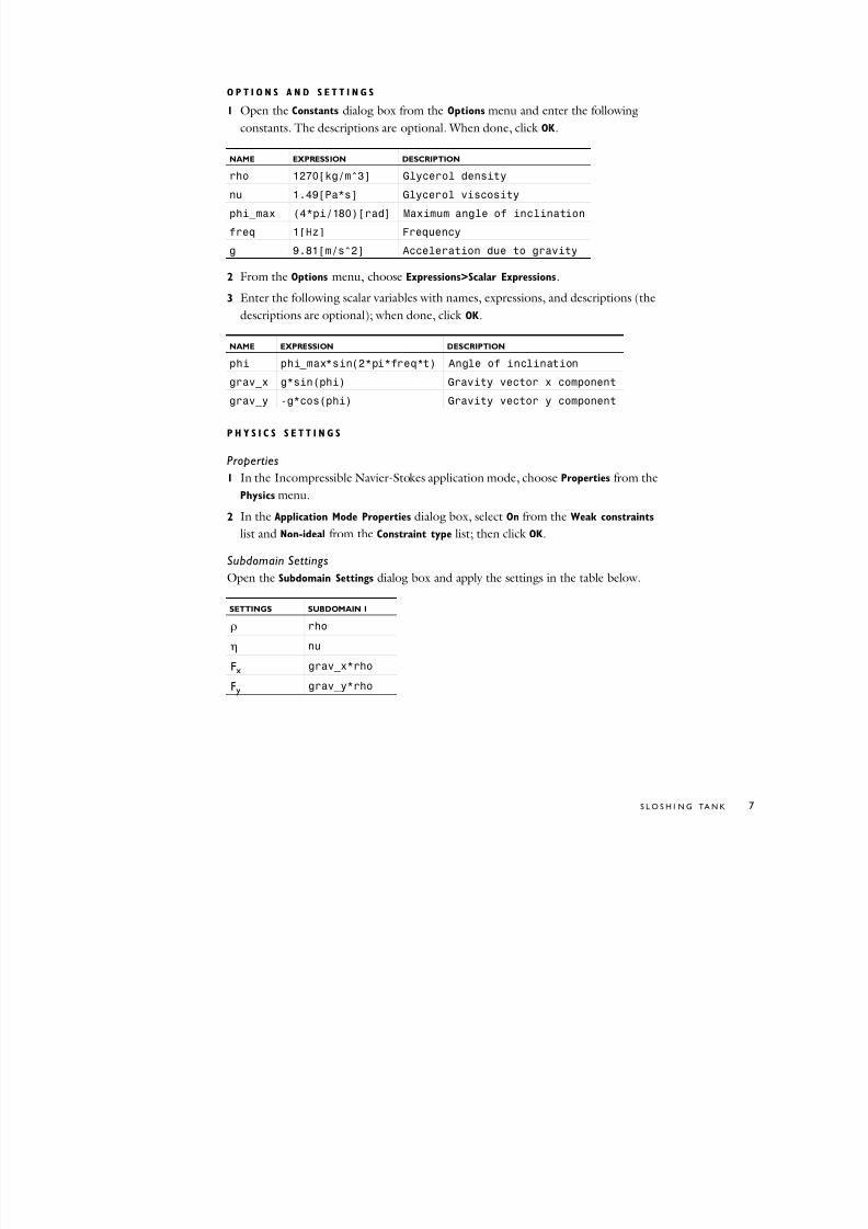
7212019 Sloshing Tank Sbs Tutorial Cosmos
httpslidepdfcomreaderfullsloshing-tank-sbs-tutorial-cosmos 810
S L O S H I N G TA N K | 7
O P T I O N S A N D S E T T I N G S
1 Open the Constants dialog box from the Options menu and enter the following
constants The descriptions are optional When done click OK
2 From the Options menu choose ExpressionsgtScalar Expressions
3 Enter the following scalar variables with names expressions and descriptions (the
descriptions are optional) when done click OK
P H Y S I C S S E T T I N G S
Properties
1 In the Incompressible Navier-Stokes application mode choose Properties from the
Physics menu
2 In the Application Mode Properties dialog box select On from the Weak constraints
list and Non-ideal from the Constraint type list then click OK
Subdomain Settings
Open the Subdomain Settings dialog box and apply the settings in the table below
NAME EXPRESSION DESCRIPTION
rho 1270[kgm^3] Glycerol density
nu 149[Pas] Glycerol viscosity
phi_max (4pi180)[rad] Maximum angle of inclination
freq 1[Hz] Frequency
g 981[ms^2] Acceleration due to gravity
NAME EXPRESSION DESCRIPTION
phi phi_maxsin(2pifreqt) Angle of inclination
grav_x gsin(phi) Gravity vector x component
grav_y -gcos(phi) Gravity vector y component
SETTINGS SUBDOMAIN 1
ρ rho
η nu
Fx grav_xrho
Fy grav_yrho
7212019 Sloshing Tank Sbs Tutorial Cosmos
httpslidepdfcomreaderfullsloshing-tank-sbs-tutorial-cosmos 910
S L O S H I N G TA N K | 8
Boundary Conditions
1 Open the Boundary Settings dialog box from the Physics menu and enter boundary
conditions according to the table below When done click OK
2 Go to the Multiphysics menu and select Moving Mesh (ALE) (ale)
3 In the Boundary Settings dialog box apply the following boundary conditions for the
mesh displacements (only tangential movements on the sides and a fixed mesh at the
bottom)
4 On Boundary 3 select Tangent and normal coord sys in deformed mesh in the
Coordinate system list Then click the Mesh velocity button and type unx+vny in
the vn edit field to specify the normal mesh velocity as u middotn
5 On the Weak Constr tab of the Boundary Settings dialog box clear the Use weak
constraints check box on Boundaries 1 2 and 4 The strong constraints that you
specified in the previous step are sufficient on these boundaries Leave the Use weak
constraints check box selected on Boundary 36 Click OK to close the dialog box
M E S H G E N E R A T I O N
Click the Initialize Mesh button on the Main toolbar to initialize the mesh
C O M P U T I N G T H E S O L U T I O N
1 Open the Solver Parameters dialog box from the Solve menu
2 Enter range(0016) in the Times edit field on the General page
3 Type 0001 in the Relative tolerance edit field This provides a 01 relative
tolerance which is one order of magnitude less than the default value
4 Click the Time Stepping tab
5 Select Exclude algebraic from the Error estimation strategy list This excludes the
pressure and the moving mesh variables from the error estimation The equations
SETTINGS BOUNDARIES 1 2 4 BOUNDARY 3
Boundary type Wall Open boundary
Boundary condition Slip Normal stress
f 0 0
SETTINGS BOUNDARIES 1 4 BOUNDARY 2
dx 0 0
dy 0
7212019 Sloshing Tank Sbs Tutorial Cosmos
httpslidepdfcomreaderfullsloshing-tank-sbs-tutorial-cosmos 1010
S L O S H I N G TA N K | 9
for those variables do not include time derivatives and become algebraic when
solving the equation system using the method of lines
6 Click OK
7 Click the Solve button on the Main toolbar
P O S T P R O C E S S I N G A N D V I S U A L I Z A T I O N
The default plot shows the x-component of the moving mesh deformation in the
spatial frame
1 To plot the velocity field of the glycerol instead go to the Surface tab in the Plot
Parameters dialog box and select Incompressible Navier-Stokes (ns)gtVelocity field
from the list of expressions
2 On the General page clear the Geometry edges check box Click Apply to see the plot
and use the Solution at time list on the General tab to browse through the output
times
You can visualize the tankrsquos inclination by clever use of the deformation plot feature
3 On the Deform page select the Deformed shape plot check box and set the Scale factor to 1 Enter Ysin(phi) in the X component edit field and -Xsin(phi) in the Y
component edit field on the Subdomain Data tab
4 Still on the Deform page click the Boundary Data tab Once again enter Ysin(phi)
in the X component edit field and -Xsin(phi) in the Y component edit field
5 On the Boundary tab select the Boundary plot check box Enter 1 in the Expression
edit field Select to use a Uniform color and pick a black color using the Color button
6 To get a more liquid-looking plot you may want to go to the Surface page and set
the Color table to GrayScale
7 Click Apply to see the plot
8 To see the waves in action go to the Animate page click Start Animation and then
click OK
To get a more comprehensive overview of the sloshing you can plot the
y-displacement from equilibrium in a point
1 Open the Domain Plot Parameters dialog box from the Postprocessing menu
2 On the Point tab select Point 4 from the Point selection list
3 Enter dy_ale in the Expression edit field then click OK to see the plot
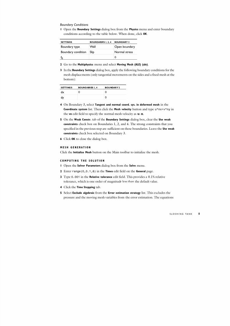
7212019 Sloshing Tank Sbs Tutorial Cosmos
httpslidepdfcomreaderfullsloshing-tank-sbs-tutorial-cosmos 910
S L O S H I N G TA N K | 8
Boundary Conditions
1 Open the Boundary Settings dialog box from the Physics menu and enter boundary
conditions according to the table below When done click OK
2 Go to the Multiphysics menu and select Moving Mesh (ALE) (ale)
3 In the Boundary Settings dialog box apply the following boundary conditions for the
mesh displacements (only tangential movements on the sides and a fixed mesh at the
bottom)
4 On Boundary 3 select Tangent and normal coord sys in deformed mesh in the
Coordinate system list Then click the Mesh velocity button and type unx+vny in
the vn edit field to specify the normal mesh velocity as u middotn
5 On the Weak Constr tab of the Boundary Settings dialog box clear the Use weak
constraints check box on Boundaries 1 2 and 4 The strong constraints that you
specified in the previous step are sufficient on these boundaries Leave the Use weak
constraints check box selected on Boundary 36 Click OK to close the dialog box
M E S H G E N E R A T I O N
Click the Initialize Mesh button on the Main toolbar to initialize the mesh
C O M P U T I N G T H E S O L U T I O N
1 Open the Solver Parameters dialog box from the Solve menu
2 Enter range(0016) in the Times edit field on the General page
3 Type 0001 in the Relative tolerance edit field This provides a 01 relative
tolerance which is one order of magnitude less than the default value
4 Click the Time Stepping tab
5 Select Exclude algebraic from the Error estimation strategy list This excludes the
pressure and the moving mesh variables from the error estimation The equations
SETTINGS BOUNDARIES 1 2 4 BOUNDARY 3
Boundary type Wall Open boundary
Boundary condition Slip Normal stress
f 0 0
SETTINGS BOUNDARIES 1 4 BOUNDARY 2
dx 0 0
dy 0
7212019 Sloshing Tank Sbs Tutorial Cosmos
httpslidepdfcomreaderfullsloshing-tank-sbs-tutorial-cosmos 1010
S L O S H I N G TA N K | 9
for those variables do not include time derivatives and become algebraic when
solving the equation system using the method of lines
6 Click OK
7 Click the Solve button on the Main toolbar
P O S T P R O C E S S I N G A N D V I S U A L I Z A T I O N
The default plot shows the x-component of the moving mesh deformation in the
spatial frame
1 To plot the velocity field of the glycerol instead go to the Surface tab in the Plot
Parameters dialog box and select Incompressible Navier-Stokes (ns)gtVelocity field
from the list of expressions
2 On the General page clear the Geometry edges check box Click Apply to see the plot
and use the Solution at time list on the General tab to browse through the output
times
You can visualize the tankrsquos inclination by clever use of the deformation plot feature
3 On the Deform page select the Deformed shape plot check box and set the Scale factor to 1 Enter Ysin(phi) in the X component edit field and -Xsin(phi) in the Y
component edit field on the Subdomain Data tab
4 Still on the Deform page click the Boundary Data tab Once again enter Ysin(phi)
in the X component edit field and -Xsin(phi) in the Y component edit field
5 On the Boundary tab select the Boundary plot check box Enter 1 in the Expression
edit field Select to use a Uniform color and pick a black color using the Color button
6 To get a more liquid-looking plot you may want to go to the Surface page and set
the Color table to GrayScale
7 Click Apply to see the plot
8 To see the waves in action go to the Animate page click Start Animation and then
click OK
To get a more comprehensive overview of the sloshing you can plot the
y-displacement from equilibrium in a point
1 Open the Domain Plot Parameters dialog box from the Postprocessing menu
2 On the Point tab select Point 4 from the Point selection list
3 Enter dy_ale in the Expression edit field then click OK to see the plot


![Sloshing motion in excited tanks - context/Earthcontextearth.com/wp-content/uploads/2016/07/JCP04.pdf · Sloshing motion in excited tanks ... [35] modelled inviscid sloshing motion](https://static.fdocuments.us/doc/165x107/5a78985e7f8b9aa2448e4299/sloshing-motion-in-excited-tanks-context-motion-in-excited-tanks-35-modelled.jpg)