S

KU

a

ARRAA

KSLFGU

1

c“ieBtptCiaicwop

aZ

n

0d

Do

Electric Power Systems Research 80 (2010) 514–527

Contents lists available at ScienceDirect

Electric Power Systems Research

journa l homepage: www.e lsev ier .com/ locate /epsr

liding mode based load-frequency control in power systems

. Vrdoljak ∗, N. Peric, I. Petrovicniversity of Zagreb, Faculty of Electrical Engineering and Computing, 10000 Zagreb, Croatia

r t i c l e i n f o

rticle history:eceived 17 April 2008eceived in revised form 28 July 2009ccepted 24 October 2009vailable online 24 November 2009

eywords:liding mode control

a b s t r a c t

The paper presents a new discrete-time sliding mode controller for load-frequency control (LFC) in controlareas (CAs) of a power system. As it uses full-state feedback it can be applied for LFC not only in CAswith thermal power plants but also in CAs with hydro power plants, in spite of their non-minimumphase behaviors. To enable full-state feedback we have proposed a state estimation method based onfast sampling of measured output variables, which are frequency, active power flow interchange andgenerated power from power plants engaged in LFC in the CA. The same estimation method is also used forthe estimation of external disturbances in the CA, what additionally improves the overall system behavior.

oad-frequency controlast output samplingenetic algorithmncertainties

Design of the discrete-time sliding mode controller for LFC with desired behavior is accomplished by usinga genetic algorithm. To the best of our knowledge, proposed controller outperforms any of the existingcontrollers in fulfilling the requirements of LFC. It was thoroughly compared to the commonly used PIcontroller by extensive simulation experiments on a power system with four interconnected CAs. Theseexperiments show that the proposed controller ensures better disturbance rejection, maintains requiredcontrol quality in the wider operating range, shortens the frequency’s transient response avoiding the

bust t

overshoot and is more ro

. Introduction

Power systems are composed of interconnected subsystems orontrol areas (CAs). Most of European countries are members ofUnion for the Co-ordination of Transmission of Electricity” (UCTE)nterconnection [1]. It is assumed that each CA consists of a coher-nt group of generators. CAs are interconnected by the tie-lines.ecause of the differences in generation and load in a power sys-em, system’s frequency deviates from its nominal value and activeower flow interchanges between areas deviate from their con-racted values. The purpose of load-frequency control (LFC) in eachA is to compensate for those deviations. That is obtained by chang-

ng power outputs of certain generators within the CA. To test LFClgorithms, an example power system is usually modeled as annterconnection of a few CAs. Since all generators in one CA areoherent, all power plants engaged in LFC in a CA can be replaced

ith one substitute power plant [2]. In some CAs that power plant is

f thermal type and in some CAs of hydro type. When modeling a CA,ower imbalance and losses can be seen as external disturbances.

∗ Corresponding author at: University of Zagreb, Faculty of Electrical Engineeringnd Computing, Department of Control and Computer Engineering, Unska 3, 10000agreb, Croatia. Tel: +385 1 6129 795; fax: +385 1 6129 809.

E-mail addresses: kresimir.vrdoljak@fer.hr (K. Vrdoljak),edjeljko.peric@fer.hr (N. Peric), ivan.petrovic@fer.hr (I. Petrovic).

378-7796/$ – see front matter © 2009 Elsevier B.V. All rights reserved.oi:10.1016/j.epsr.2009.10.026

wnloaded from http://www.elearnica.ir

o uncertainties in the system.© 2009 Elsevier B.V. All rights reserved.

Nowadays, in the majority of CAs PI type controllers with con-stant parameters are used for LFC [3–6]. However, systems with PIcontrol have long settling time and relatively large overshoots infrequency’s transient responses [7]. Besides, PI control algorithmprovides required behavior of the system only in the vicinity ofthe nominal operating point, for which it is designed. But, oper-ating point of a power system usually changes a lot, which isprimarily caused by the amount and characteristic of power con-sumption, characteristics of power plants and the number of powerplants engaged in LFC in a CA. Future power systems will rely onlarge amounts of distributed generation with large percentage ofrenewable energy based sources, what will further increase sys-tem uncertainties and thereby induce new requirements to the LFCsystem [8]. The shortening of time periods in which each level of fre-quency regulation must finish could be also expected in the future[9].

Therefore, an advanced controller should be developed and usedinstead of the PI controller in order to: (1) ensure better distur-bance rejection, (2) maintain required control quality in the wideroperating range, (3) shorten the frequency’s transient responsesavoiding the overshoots and (4) be robust to uncertainties in thesystem. Additionally, a new control algorithm for a CA should

enable decentralized LFC of interconnected CAs, i.e. its structureand parameters must not depend on applied controllers in neigh-boring CAs. It should also be a discrete-time control algorithm withsampling time in the range 1–5 s as required in UCTE intercon-nection [1]. Finally, it should be relatively simple to implement,

System

ia

ftcptSaficst[([inf

ttrl[mgrip

c(Bodpdskisltofr

soapboeftsui

peS

xi(t) =⎢⎢⎢⎢⎣

tiei

�Pgi(t)

�xgi(t)

�xghi(t)

⎥⎥⎥⎥⎦ , di(t) = �Pdi(t). (2)

K. Vrdoljak et al. / Electric Power

n order to be accepted as adequate replacement of PI controllgorithm.

Recently, many different control algorithms have been proposedor LFC [10,11] in order to overcome limitations of the PI con-roller. Among them, the most immanent are based on: robustontrol, [5,12], fuzzy logic [13–15], neural networks [16–18], modelredictive control [19,20], optimal control [21–23], adaptive con-rol [24–26] and sliding mode control (SMC) [27–31] algorithms.ome drawbacks present in the above algorithms can be listeds follows: (1) measurements from neighbor CAs are requiredor controller synthesis, but obtaining them could be impracticaln real power system [25,27]; (2) control signal is computed inontinuous-time [5,15,27–32] although in real power system theignal should be sent to the power plants in discrete-time; (3) con-rollers are based on full system state, but with no estimator present14,22,27–31]; (4) controllers are complex and of high order [20];5) there is a requirement for on-line parameters identification24,30]; (6) the choosing of appropriate controller parameterss problematic [23,29,32]. Listed drawbacks clearly indicate thatone of the abovementioned controllers fulfills all requirements

or LFC.In this paper we propose a discrete-time sliding mode controller

hat at best of our knowledge outperforms any of the existing con-rollers in fulfilling the requirements for LFC. Generally, SMC is aobust control technique that shows very good behavior in control-ing systems with external disturbances and parameter variations33]. In SMC, system closed-loop behavior is determined by a sub-

anifold in the state space, which is called a sliding surface. Theoal of the sliding mode control is to drive the system trajectory toeach the sliding surface and then to stay on it. When the trajectorys on the surface, system invariance to particular uncertainties andarameter variations is guaranteed.

Ideal sliding of the system trajectory along the sliding surfacean be achieved only by the continuous-time SMC with very hightheoretically infinite) switching frequency of the control signal.ut, real power plants are unable to respond to so fast changesf the control signal, and that is the reason why we propose aiscrete-time sliding mode controller which changes control signaleriodically in discrete-time instants. Of course, with the usage ofiscrete-time SMC the system trajectory can’t be kept on the slidingurface but inside a small band around the surface. That behavior isnown as quasi sliding mode [34]. Two main problems in design-ng discrete-time SMC for LFC are appropriate choices of slidingurface which defines desired system behavior, and of reachingaw which must be chosen to ensure convergence of the trajec-ory from any point in the state space towards the surface [35]. Anptimization method based on genetic algorithm (GA) is proposedor finding optimal parameters of the sliding surface and of theeaching law.

If only thermal power plants are used for LFC in a CA then stableliding mode controller can be also designed using only measuredutput signals, which are frequency, active power flow interchangend generated power from each power plant in that CA. But, if hydroower plants are used for LFC then full-state feedback is neededecause of their non-minimum phase behaviors. We have devel-ped a full-state sliding mode controller, which can be applied inither cases. The usage of the state estimation method based onast output sampling (FOS) [36] is proposed, what is possible dueo availability of multiple measurements of output signals in eachampling period of the controller. FOS estimation method is alsosed for the estimation of external disturbances, what additionally

mproves the overall system behavior.The brief outline of the paper is as follows: Section 2 presents

ower system model, Section 3 describes state and disturbancestimation technique. Section 4 gives an overview of discrete-timeMC and its application to LFC. Section 5 presents a GA used for

s Research 80 (2010) 514–527 515

the purpose of finding optimal sliding mode algorithm parameters,while Section 6 contains simulation results.

2. Mathematical model of a power system

An example mathematical model of a power system used in thispaper consists of four interconnected CAs, each represented withone substitute thermal or hydro power plant. Each CA has its ownload frequency controller, as it is shown in Fig. 1. Power system ismodeled as continuous, while control signals are sent to the plantsin discrete-time.

It is supposed that power plants in CA1 and CA4 are thermalpower plants, while power plants in CA2 and CA3 are hydro powerplants. Furthermore, power plants in CA1 and CA2 have less gener-ating capacity then those in CA3 and CA4. Sliding mode based LFC,described in Section 4, will be applied to CA1 and CA3, while LFC inother CAs will be based on conventional PI type control algorithm.

Linearized mathematical model of each of four CAs can bedescribed with the following equation:

xi(t) = Aixi(t) +∑

j

Aijxj(t) + Biui(t) + Fidi(t) + �i(x, u, t), (1)

where xi ∈Rn is the system state vector, xj ∈Rp is a state vectorof the neighbor system, ui ∈Rm is the control signal vector, di ∈Rk

is the disturbance vector, �i is a vector of uncertainties and y ∈Rl

is the output vector. Matrices in (1) have appropriate dimensions:Ai ∈Rn×n, Aij ∈Rn×p, Bi ∈Rn×m, Fi ∈Rn×k and Ci ∈Rl×n.

Linearized model of CAs are used instead of the nonlinear onesbecause proposed SMC is based on such a linear model, wherelinearization error is included in the uncertainty term �i(x, u, t).Simplified linearized continuous-time models of CAs with one sub-stitute hydro or thermal power plant are shown in Figs. 2 and 3,respectively.

For the model shown in Fig. 2 state and disturbance vectors from(1) are (see Table 1):⎡

⎢ �fi(t)

�P (t)

⎤⎥

Fig. 1. Four interconnected control areas.

516 K. Vrdoljak et al. / Electric Power Systems Research 80 (2010) 514–527

l area

w

˛

Mwcm

Fig. 2. The block diagram of i-th contro

Matrices in (1) are:

Ai =

⎡⎢⎢⎢⎢⎢⎢⎢⎢⎢⎢⎢⎢⎢⎣

− 1TPi

−KPi

TPi

KPi

TPi0 0∑

j

KSij 0 0 0 0

2˛ 0 − 2TWi

2� 2ˇ

−˛ 0 0 − 1T2i

−ˇ

− 1T1iRi

0 0 0 − 1T1i

⎤⎥⎥⎥⎥⎥⎥⎥⎥⎥⎥⎥⎥⎥⎦

,

Bi =

⎡⎢⎢⎢⎢⎢⎢⎢⎣

0

0

−2Riˇ

Riˇ

1T1i

⎤⎥⎥⎥⎥⎥⎥⎥⎦

, Fi =

⎡⎢⎢⎢⎢⎢⎢⎢⎣

−KPi

TPi

0

0

0

0

⎤⎥⎥⎥⎥⎥⎥⎥⎦

,

(3)

ith coefficients:

= TRi

T1iT2iRi, ˇ = TRi − T1i

T1iT2i, � = T2i + TWi

T2iTWi. (4)

atrices Aij in (1) have dimensions 5 × 4 or 5 × 5, depending onhether they are used to describe hydro–thermal or hydro–hydro

onnection. All of their elements are equal to zero, except the ele-ent at position (1, 2), which is equal to −KSij .

Fig. 3. The block diagram of i-th control area

represented with hydro power plant.

For the model shown in Fig. 3 state and disturbance vectors from(1) are:

xi(t) =

⎡⎢⎢⎢⎣

�fi(t)

�Ptiei(t)

�Pgi(t)

�xgi(t)

⎤⎥⎥⎥⎦ , di(t) = �Pdi(t), (5)

while matrices in (1) are:

Ai =

⎡⎢⎢⎢⎢⎢⎢⎢⎢⎢⎢⎣

− 1TPi

−KPi

TPi

KPi

TPi0∑

j

KSij 0 0 0

0 0 − 1TTi

1TTi

− 1TGiRi

0 0 − 1TGi

⎤⎥⎥⎥⎥⎥⎥⎥⎥⎥⎥⎦

,

Bi =

⎡⎢⎢⎢⎢⎣

0

0

0

1TGi

⎤⎥⎥⎥⎥⎦ , Fi =

⎡⎢⎢⎢⎢⎣

−KPi

TPi

0

0

0

⎤⎥⎥⎥⎥⎦ .

(6)

In this case, matrices Aij in (1) have dimensions 4 × 4 or 4 × 5,

depending on whether they are used to describe thermal–thermalor thermal–hydro connection. Again, all of their elements are equalto zero, except the element at position (1, 2), which is equal to −KSij .

Signals and parameters used in the models from Figs. 2 and 3are shown in Table 1.

represented with thermal power plant.

K. Vrdoljak et al. / Electric Power Systems Research 80 (2010) 514–527 517

Table 1Power system variables and parameters.

Parameter/variable Description Unit

�f (t) Frequency deviation Hz�Pg (t) Generator output power deviation p.u.MW�xg (t) Governor valve position deviation p.u.�xgh(t) Governor valve servomotor position deviation p.u.�Ptie(t) Tie-line active power deviation p.u.MW�Pd(t) Load disturbance p.u.MW�ı(t) Rotor angle deviation radKP Power system gain Hz / p.u.MWTP Power system time constant sTW Water starting time sT1, T2, TR Hydro governor time constants sTG Thermal governor time constant sTT Turbine time constant sK Interconnection gain between CAs p.u.MW

fdbiCp(

y

weat

pp

3

bf

Lv

cws

M

S

KB Frequency bias factor p.u.MW / HzR Speed droop due to governor action Hz / p.u.MWACE Area control error p.u.MW

UCTE prescribes a set of rules and recommendations about LFCor its members. Thereby, an area control error (ACE) signal is intro-uced as a quantitive measure of CA’s deviation from the proposedehavior. ACE is defined as a combination of frequency deviation

n a CA and of active power flow deviation in tie-lines connecting aA with the neighbor areas. The goal of LFC in each area is to com-ensate for ACE deviations. Therefore, let the output of the system1) be defined as:

i(t) = Cixi(t) = ACEi(t) = KBi�fi(t) + �Ptiei(t), (7)

here parameter KB is tuned in a way that ensures ACE differ-nt than zero only for a CA in which the disturbance occurs. Inll other CAs, values of ACE signals are not significantly affected byhat disturbance.

Matrix Ci in (7) is Ci = [ KBi 1 0 0 0 ] for a CA with hydroower plant and Ci = [ KBi 1 0 0 ] for a CA with thermal powerlant.

. System state and disturbance estimation

A general continuous-time linear system with added distur-ance and neglected uncertainties can be described with theollowing equations:

x(t) = Ax(t) + Bu(t) + Fd(t),

y(t) = Cx(t).(8)

et us assume that control signal u from (8) is able to change itsalue only every � seconds, where � is a sampling period.

In order to design discrete-time estimator, system (8) is dis-retized using the Zero-Order-Hold (ZOH) discretization method,ith sampling period �. That results in the following discrete-time

ystem:

x((k + 1)�) = G�x(k�) + H�u(k�) + W�d(k�),

y(k�) = Cx(k�).(9)

atrices in (9) are defined as follows:

G� = eA�,

H� =�∫

eAtBdt,

0

W� =�∫0

eAtFdt.

(10)

Fig. 4. The usage of the FOS estimation method in system control.

Let us also assume that only system output is measurable, andonly at certain time instances, y(kT), where T is a subsamplingperiod:

T = �

N, (11)

where N ∈N. Those samples can be used as input signals of theappropriate estimator for unmeasured state and disturbance sig-nals in (8).

LFC applied nowadays in real power systems is an exam-ple of a system with multiple sampling periods. In LFC, controlsignal is sent to the power plants in discrete-time. In UCTEinterconnection that period is 1–5 s [6]. Additionally, during onesampling period several measurements of frequency f (kT) andtie-line power Ptie(kT) signals are gathered. Besides those sub-samples, which are inputs to classical PI controller, subsamplesof generated power Pg(kT) are also gathered for monitoring pur-poses. Those samples could also be used as inputs to the estimator.Because a substitute power plant is used in modeling a CA andalso in controller synthesis, all other state and disturbance sig-nals, that cannot be measured in the real system, must therefore beestimated.

3.1. Fast output sampling method

Fast output sampling (FOS) is an estimation technique appro-priate for continuous time system controlled with discrete-timecontrol signal, where the output signal can be sampled severaltimes during one period of the control signal [36]. FOS showsbetter performance than standard estimation techniques, becauseit reduces the estimation error to zero after just one samplingperiod [34]. Standard estimators need at least � sampling periodsto achieve errorless estimation, where � is the observability indexof the system [37]. To use FOS estimation technique, it must besatisfied N ≥ � [36].

The principle of using FOS estimation technique in systemcontrol is shown in Fig. 4. Firstly, the last N subsamples of the

output signal y(t), measured in the most recent sampling period�, are used to estimate the system state. Then, that estimatedstate is used to compute the control signal for the next samplingperiod.

5 System

Ittpw

idu

p

vsdti

slp

y

N

y

18 K. Vrdoljak et al. / Electric Power

Consider system (8), sampled at subsampling period T:

x((k + 1)T) = GT x(kT) + HT u(kT) + WT d(kT),

y(kT) = Cx(kT).(12)

t should be noted that system (12) has different sampling periodhan system (9). Its matrices GT , HT and WT are defined similar tohose in (10), just with subsampling period T instead of samplingeriod �. Relation between those two sampling periods is givenith (11).

System with fast output sampling can be described by combin-ng (9) and (12). Generally, let the input vector of that system beecoupled into two components: u� (with sampling period �) andT (with subsampling period T).

The system’s N consecutive subsamples, taken during the sam-ling period �, can now be calculated as:

x(k� + T) = GT x(k�) + HT (u�(k�) + uT (k�))

+WT d(k�),

x(k� + 2T) = G2T x(k�) + (GT HT + HT )u�(k�)

+GT HT uT (k�) + HT uT (k� + T)

+(GT WT + WT )d(k�),

...

x(k� + (N − 1)T) = GN−1T x(k�) +

N−2∑i=0

(GiT HT )u�(k�)

+ GN−2T HT uT (k�)

+GN−3T HT uT (k� + T) + . . .

+HT uT (k� + (N − 2)T)

+N−2∑i=0

(GiT WT )d(k�).

(13)

It is assumed here that the disturbance d(k�) has a constantalue during the whole sampling period �. That assumption is rea-onable for LFC because in real power systems changes of �Pd(t)uring one sampling period � can be neglected. It is also assumedhat there is no direct influence of input signal to system’s output,.e. D = 0.

A procedure to estimate unmeasured state and disturbancetarts from a vector of output subsamples y∗

k, which consists of the

ast N output subsamples, sampled in the most recent samplingeriod �. It is:

∗k =

⎡⎢⎢⎢⎢⎢⎢⎢⎢⎢⎣

y(k�)

y(k� + T)

y(k� + 2T)

...

y(k� + (N − 2)T)

y(k� + (N − 1)T)

⎤⎥⎥⎥⎥⎥⎥⎥⎥⎥⎦

. (14)

ow from (9), (13) and (14) it follows:

∗k = Gx(k�) + Hu�(k�) + Hu∗

k + Wd(k�), (15)

s Research 80 (2010) 514–527

where

u∗k

=

⎡⎢⎢⎢⎢⎢⎢⎢⎢⎢⎣

uT (k�)

uT (k� + T)

uT (k� + 2T)

...

uT (k� + (N − 3)T)

uT (k� + (N − 2)T)

⎤⎥⎥⎥⎥⎥⎥⎥⎥⎥⎦

, G =

⎡⎢⎢⎢⎢⎢⎢⎢⎢⎢⎢⎣

C

CGT

CG2T

...

CGN−2T

CGN−1T

⎤⎥⎥⎥⎥⎥⎥⎥⎥⎥⎥⎦

,

H =

⎡⎢⎢⎢⎢⎢⎢⎢⎢⎢⎢⎢⎢⎢⎢⎢⎢⎣

0

CHT

C(GT HT + HT )

...

CN−3∑i=0

GiT HT

CN−2∑i=0

GiT HT

⎤⎥⎥⎥⎥⎥⎥⎥⎥⎥⎥⎥⎥⎥⎥⎥⎥⎦

, W =

⎡⎢⎢⎢⎢⎢⎢⎢⎢⎢⎢⎢⎢⎢⎢⎢⎢⎣

0

CWT

C(GT WT + WT )

...

CN−3∑i=0

GiT WT

CN−2∑i=0

GiT WT

⎤⎥⎥⎥⎥⎥⎥⎥⎥⎥⎥⎥⎥⎥⎥⎥⎥⎦

,

H =

⎡⎢⎢⎢⎢⎢⎢⎢⎢⎢⎣

0 0 · · · 0 0

CHT 0 · · · 0 0

CGT HT CHT · · · 0 0

......

. . ....

...

CGN−3T HT CGN−4

T HT · · · CHT 0

CGN−2T HT CGN−3

T HT · · · CGT HT CHT

⎤⎥⎥⎥⎥⎥⎥⎥⎥⎥⎦

.

(16)

Matrices G and W may not be square, so Eq. (15) could have multi-ple solutions. In that case, Moore-Penrose matrix pseudoinverse isused in estimation algorithm instead of the regular inverse. Pseu-doinverse of matrix M is defined as [38]:

M+ = (MT M)−1

MT . (17)

Eq. (15) can be directly used only for disturbance estimation:

d(k�) = W+ (

y∗k − Gx(k�) − Hu�(k�) − Hu∗

k

), (18)

The usage of matrix’s pseudoinverse will ensure that estimatedvalues represent the least square solution of (15) [39].

Nevertheless, if Eq. (15) is also used for state estimation, esti-mated value would be delayed one sampling period �. Therefore, forstate estimation, that equation is combined with discrete systemsdynamics (9), which results in the following state estimation:

x((k + 1)�) = G� G+

y∗k

+ H�u�(k�) − G� G+

Hu∗k

+H◦u◦k + (W� − G� G

+W)d(k�),

(19)

where

H◦ = [GN−1T HT GN−2

T HT · · · GT HT HT ],

◦

⎡⎢⎢⎢⎢⎢

uT (k�)

uT (k� + T)

uT (k� + 2T)

⎤⎥⎥⎥⎥⎥ (20)

u k = ⎢⎢⎢⎢⎣...

uT (k� + (N − 2)T)

uT (k� + (N − 1)T)

⎥⎥⎥⎥⎦.

K. Vrdoljak et al. / Electric Power Systems Research 80 (2010) 514–527 519

system for state estimation.

3

hstTsiBmT

w

t(sh

w

cb

TS

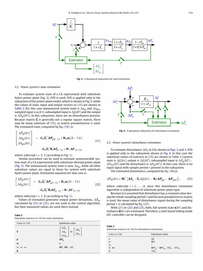
Fig. 5. A dynamical sub

.2. Power system’s state estimation

To estimate system state of a CA represented with substituteydro power plant (Fig. 2), FOS is used. FOS is applied only to theubsystem of the power plant model, which is shown in Fig. 5, whilehe values of state, input and output vectors in (15) are shown inable 2 (for this case unmeasured system state is �xgi and �xghi,ampled input is ui(k�), subsampled input is �fi(kT) and the outputs �Pgi(kT)). In this subsystem, there are no disturbances present.ecause matrix G is generally not a regular square matrix, thereay be many solutions of (15), so matrix pseudoinverse is used.

he estimated state, computed by Eq. (19), is:⎡⎢⎣

�Pgi(k�)

�xgi(k�)

�xghi(k�)

⎤⎥⎦ = G�iG

+i �P∗

g(k−1)i + H�iui((k − 1)�)

−G�iG+i Hi�f∗

(k−1)i + H◦i�f◦

(k−1)i,

(21)

here subscript i = 2, 3 (according to Fig. 1).Similar procedure can be used to estimate unmeasurable sys-

em state of a CA represented with substitute thermal power plantFig. 3). The unmeasured system state is now �xgi, while all otherubstitute values are equal to those for system with substituteydro power plant. Estimation equation for that case is:[�Pgi(k�)

�xgi(k�)

]= G�iG

+i �P∗

g(k−1)i + H�iui((k − 1)�)

−G�iG+i Hi�f∗

(k−1)i + H◦i�f◦

(k−1)i,

(22)

here subscript i = 1, 4 (according to Fig. 1).Values of estimated generator output power deviations, �Pgi,

alculated by (21) or (22), are not used in the control algorithm,ut their measured values are used there instead.

able 2ubstitute matrices in (19) for state estimation.

Value in (19) Substitute value

x

[�Pgi

�xgi

�xghi

]or

[�Pgi

�xgi

]y∗ �P∗

gi

u� ui

u∗,u◦,uT �f∗i , �f◦

i, �fi

d –

Fig. 6. A dynamical subsystem for disturbance estimation.

3.3. Power system’s disturbance estimation

To estimate disturbance �Pd in CAs shown in Figs. 2 and 3, FOSis applied only to the subsystem shown in Fig. 6. In this case thesubstitute values of matrices in (15) are shown in Table 3 (systemstate is �fi(k�), output is �fi(kT), subsampled input is �Pgi(kT) −�Ptiei(kT) and the disturbance is �Pdi(kT)). In this case, there is noinput signal with sample period � present in the subsystem.

The estimated disturbance, computed by Eq. (18),is:

�Pdi(k�) = W+i

[�f∗

ki − Gi�fi(k�) − Hi(�P∗gki − �P∗

tieki)]

, (23)

where subscript i = 1, . . . , 4, since this disturbance estimationalgorithm is independent of substitute power plant type.

Because it is assumed that disturbance has a constant value dur-ing the whole sampling period � and because pseudoinverse matrixis used, the mean value of disturbance signal during the samplingperiod � is calculated by Eq. (23).

With (21) or (22) and (23), both, full system state x(k�) and dis-turbance d(k�) are estimated. Therefore, a state based sliding modeLFC controller can be designed.

Table 3Substitute matrices in (18) for disturbance estimation.

Value in (18) Substitute value

x �fiy∗ �f ∗

iu� –u∗, uT �P∗

gi− �P∗

tiei, �Pgi − �Ptiei

d �Pdi

5 Systems Research 80 (2010) 514–527

4L

ctsitftBtc

4

tads

d

x

Oou

�

wm

�

w

ps

wsd

tc

nt

Ss

20 K. Vrdoljak et al. / Electric Power

. Discrete-time sliding mode control and its application toFC

Sliding mode control is a control technique appropriate forontrolling time-variant systems in the presence of external dis-urbances. SMC based only on output signal cannot be used forystems with non-minimum phase behavior, because it leads tonstability [35]. As seen from Fig. 2, a hydro power plant is a sys-em with non-minimum phase behavior. Therefore, SMC based onull system state must be used in this case. To improve overall sys-em behavior, disturbance is also included into controller’s design.ecause all state and disturbance are not measurable, estimationechnique described in Section 3 is used to obtain their unmeasuredomponents.

.1. Sliding mode control for systems with uncertainties

Eq. (8) describes a linear time-invariant (LTI) system model inhe presence of external disturbance. But in real systems therere many uncertainties present, which are caused by unmodelledynamics or variations of system parameters. They can highly affectystem’s behavior.

A continuous LTI system (8) with additive uncertainties isescribed as:

˙ (t) = Ax(t) + Bu(t) + Fd(t) + �(x, u, t). (24)

ne way to categorize uncertainties in the system is into matchedr unmatched uncertainties [40]. A condition that defines matchedncertainties is:

m(x, u, t) ∈R(B), (25)

hereas all other uncertainties are unmatched. Because of theatching condition (25), matched uncertainties can be written as:

m(x, u, t) = B�, (26)

here � ∈Rm [40].For better insight into system dynamics with SMC and for sim-

ler controller synthesis it is more convenient to transform theystem (24) into a regular canonical form [33]:[

xc1(t)

xc2(t)

]=[

A11 A12

A21 A22

][xc1(t)

xc2(t)

]+[

0

B2

]u(t)

+[

F1

F2

]d(t) +

[�u(x, t)

�m(x, u, t)

],

(27)

here xc1 and xc2 represent state vectors of the decoupled sub-ystems of system (24). In regular form system’s uncertainties areecoupled into matched and unmatched ones.

As it can be seen from (27), the influence of matched uncer-ainties in continuous SMC can be fully compensated with properontrol signal, which is not the case for unmatched uncertainties.

System’s transformation into regular form can be done withonsingular transformation matrix Tcr , where matrices defining theransformed system can be obtained from the original system as:

xcr(t) =[

xc1(t)

xc2(t)

]= Tcrx(t),

Ar =[

A11 A12

A21 A22

]= TcrAT−1

cr ,

[ ] [ ](28)

Br =0

B2= TcrB, Fr =

F1

F2= TcrF.

MC design procedure is shown in Fig. 7. It consists of two majorteps: (1) selecting a sliding surface and (2) computing a control

Fig. 7. SMC computation scheme.

law that will force system’s trajectory towards the chosen surface.A sliding surface will be selected for continuous time system in reg-ular form, because then sliding surface’s dependency upon systemparameters in (3) or (6) is preserved. Because of the controller’sdiscrete-time implementation, a control law will be computed fordiscrete-time system in regular form.

4.2. A sliding surface

The first step in SMC controller synthesis is choosing a slidingsurface, which defines desired system dynamics:

�(x) = Sx = 0, (29)

where S ∈Rm×n is a switching matrix.The aim of SMC is to force the state, firstly to reach, and then to

stay on the sliding surface. According to that, system trajectory inSMC consists of two phases: a reaching phase and a sliding phase.SMC is forcing system’s trajectory towards the surface by switchingbetween different controller structures, depending on the sign of aswitching function. The switching function is defined as:

�(t) = Sx(t). (30)

It is important to distinguish the sliding surface �(x) = 0, whichis time-independent manifold in state space and the switchingfunction �(t), which is time-dependent function of system state’sposition regarding to the sliding surface.

For the system in regular form (27), switching functionbecomes:

�(t) = Sc1xc1(t) + Sc2xc2(t), (31)

where

Scr =[

Sc1 Sc2]

= ST−1cr . (32)

System dynamics in the sliding mode are obtained from (27) and(31):

[xc1(t)

]=[

A11 A12

][x1(t)

]+[

0]

u(t)

�(t) A21 A22 �(t) B2

+[

F1

F2

]d(t) +

[�u(x, t)

�s(x, u, t)

].

(33)

System

w

Twd

t

x

Fiosi

Rfhscv

ii

ssTme

4

m

x

wliTc

a

�

w

S

K. Vrdoljak et al. / Electric Power

here

A11 = A11 − A12S∗c,

A12 = A12S−1c2 ,

A21 = Sc1A11 − Sc1A12S∗c + Sc2A21 − Sc2A22S∗

c,

A22 = Sc1A12S−1c2 + Sc2A22S−1

c2 ,

B2 = Sc2B2,

F2 = Sc1F1 + Sc2F2,

�s(x, u, t) = Sc1�u(x, t) + Sc2�m(x, u, t),

S∗c = S−1

c2 Sc1.

(34)

he term �s(x, u, t) in (33) and (34) denotes sliding uncertainties,hich can be defined as the total influence of uncertainties to theynamics of reaching the sliding mode.

Including the condition for sliding mode (�(t) = 0) into the sys-em (33), the dynamics of the system in sliding mode become:

˙ c1(t) = A11x1(t) + F1d(t) + �u(x, t). (35)

rom (35) two improvements in system behavior can be noted. Ones that the order of system dynamics is reduced compared to theriginal system (27). The reduction factor is m, which is a dimen-ion of the control signal u(t). The other improvement is system’snvariance to matched uncertainties, as they are not present in (35).

emark 1. For discrete-time systems those improvements are notully valid. Due to discrete control signal, system trajectory can not beeld strictly on the surface and matched uncertainties can influence theystems dynamics. Nevertheless, if the boundedness of uncertainties isonserved, system trajectory will maintain inside a narrow band in theicinity of the sliding surface.

Switching matrix S in (29) must be chosen such that the systemn sliding mode is stable, i.e. all eigenvalues of matrix A11 must ben the left complex halfplane.

In LFC it is required for system output i.e. ACE signal in steadytate to be equal to zero. In sliding mode system output in steadytate depends upon parameters of the switching matrix S [41].herefore, besides ensuring system’s stability in sliding mode,atrix S should be chosen such to minimize system’s steady state

rror.

.3. A control law

A control law will be computed for discrete-time ZOH approxi-ation of continuous-time LTI system with uncertainties (24):

((k + 1)�) = Gx(k�) + Hu(k�) + Wd(k�) + �(x, u, k�), (36)

here matrices G, H and W are obtained from (10). For controlaw computation discrete-time systems (36) is firstly transformednto regular form using nonsingular transformation matrix Tr .ransformation procedure is similar to the one described forontinuous-time system.

For the system in regular form, the switching function is defineds:

(k�) = S1x1(k�) + S2x2(k�), (37)

here

r =[

S1 S2]

= ST−1r . (38)

s Research 80 (2010) 514–527 521

Combining discrete-time system in regular form and Eq. (37), sys-tem dynamics in the sliding mode are obtained as:[

x1((k + 1)�)

�((k + 1)�)

]=[

G11 G12

G21 G22

][x1(k�)

�(k�)

]+[

0

H2

]u(k�)

+[

W1

W2

]d(k�) +

[�u(x, k�)

�s(x, u, k�)

].

(39)

where

G11 = G11 − G12S∗,

G12 = G12S−12 ,

G21 = S1G11 − S1G12S∗ + S2G21 − S2G22S∗,

G22 = S1G12S−12 + S2G22S−1

2 ,

H2 = S2H2,

W2 = S1W1 + S2W2,

�s(x, u, k�) = S1�u(x, k�) + S2�m(x, u, k�)

S∗ = S−12 S1.

(40)

The control law will be computed according to (39), by an appro-priate choice of a reaching law. The reaching law is in charge ofdriving system trajectory to the sliding surface �(x) = 0. Amongseveral known reaching laws [42–46], a linear reaching law from[46] is chosen to be used for LFC. It is defined as:

�(k + 1) = ��(k), (41)

where � is a diagonal matrix whose elements are constrained to0 ≤ �i < 1.

When applied to the system (39) and with neglected uncertain-ties, reaching law (41) results with the following control law:

u(k�) = H−12

[(� − G22)�(k�) − G21x1(k�) − W2d(k�)

]. (42)

Because uncertainties are neglected in the computation of the con-trol law (42), the ideal sliding mode is not guaranteed. Instead ofthat, system trajectory will reside in a quasi sliding mode band,whose width, wb, depends upon the value of components of slidinguncertainties vector, �s(x, u, k�), and also upon the parameters ofmatrix � [35]:

wb =

√√√√ m∑i=1

(1

1 − �imax(�si(x, k�))

). (43)

As stated above, in LFC state and disturbance are not fully mea-surable, therefore their unmeasured values in (42) are substitutedwith the estimated values. Estimated states are obtained by (21) or(22), while estimated disturbances are obtained by (23). Estimatedvalues are not exactly equal to the true values. The differencesare caused by discretization (9) and by least square approxima-tion which is obtained when matrix’s pseudoinverse (17) is used.They are further included into the computation of control signal(42). Because those errors can also be seen as uncertainties in (24),their influence can be reduced by introducing sliding uncertaintiesestimation term into (42). Thus, the control law becomes:

u(k�) = H−12

[(� − G22)�(k�) − G21x1(k�) − W2d(k�) − �s(k�)

],

(44)

where

�s(k�) = �s((k − 1)�) + �(k�) − ��((k − 1)�). (45)

5 System

Wtb

w

wsuos

si

4

R1b(

p

S

wp

S

TeiL

eaabc

pcpT

T

S(i

A

w

C

(

22 K. Vrdoljak et al. / Electric Power

hen sliding uncertainties estimation is included into the con-rol law computation, the width of the quasi sliding mode bandecomes [35]:

b =

√√√√ m∑i=1

(1

1 − �imax(��si(x, k�))

), (46)

here ��si(x, k�) = |�si(x, (k + 1)�) − �si(x, k�)|. The width of quasiliding mode band in (43) is based on the maximal value of slidingncertainties, while the width in (46) is based on the maximal ratef change of sliding uncertainties. Generally, the width (46) is muchmaller.

Since the main task of the sliding mode controller is to steer theystem towards the sliding surface, estimating sliding uncertaintiesnstead of all system uncertainties is enough to obtain that task.

.4. SMC application to LFC

emark 2. Because control signal in LFC has dimension one (m =, u ≡ u), there is only one sliding surface. Therefore, switching matrixecomes a switching vector while reaching law matrix becomes a scalar� ≡ �).

According to (2), a switching vector for a CA with hydro powerlant is:

=[

sf sPtie sPg sxg sxgh

], (47)

hile according to (5), a switching vector for a CA with thermalower plant it is:

=[

sf sPtie sPg sxg

]. (48)

he choice of parameters of switching vectors (47) and (48) mustnsure system’s stability in the sliding mode and it must also min-mize ACE deviation in the steady state, which is the main goal ofFC.

Minimization of ACE in steady state sliding mode can be doneither analytically [41,47] or with the usage of iterative heuristiclgorithms [7,48]. In this paper, steady state ACE will be minimizednalytically. Minimization procedure results in constraints that wille later incorporated into a genetic algorithm in charge of findingontroller’s optimal parameters (see Section 5).

The constraints will be computed separately for a CA with hydroower plant and for a CA with thermal power plant. To compute theonstraints, the systems must be in regular form. A CA with thermalower plant, described with (6), is already in regular form, thereforecr = I. For a CA with hydro power plant transformation matrix is:

cr =

⎡⎢⎢⎢⎢⎢⎢⎢⎣

KB 1 0 0 0

0 1 0 0 0

0 0 1 2 0

0 0 0 1 −TR

T2

0 0 0 0 1

⎤⎥⎥⎥⎥⎥⎥⎥⎦

. (49)

teady state ACE for system in regular form can be computed using35) and neglecting uncertainties. In sliding mode’s steady state its xc1(t) = 0, therefore ACE becomes:

CEss = −C1A−111 F1d(t), (50)

here

r =[

C1 C2]

= CT−1cr . (51)

s Research 80 (2010) 514–527

For ACEss to be equal to zero for system in sliding mode regardlessthe value of disturbance, parameters of the switching vector mustbe chosen such that they ensure:

C1A−111 F1 = 0. (52)

Solving (52) for a CA with hydro power plant, the switching vector(47), and the transformation matrix (49) gives:

sPg + sxg + sxgh = 0,sPtie /= 0.

(53)

Similarly, solving (52) for a CA with thermal power plant and theswitching vector (48), while having in mind Tcr = I, gives:

sPg + sxg = 0,sPtie /= 0.

(54)

Inequality sPtie /= 0 in (53) and (54) is a constraint introduced toavoid undefined solution of (52), ACEss = 0/0.

Altogether, parameters of the switching vector S must be chosensuch that matrix A11 is a Hurwitz matrix, while condition (53) or(54) must also be fulfilled.

5. GA for finding LFC controller’s parameters

As it can be seen from (38), (40) and (44), apart from systemparameters, control law depends on switching vector S and reach-ing law parameter �. To determine their optimal values GA is used.

GA is a random search approach which imitates natural processof evolution. It is appropriate for finding global optimal solutioninside a multidimensional searching space. GAs have been used tofind parameters for different LFC algorithms, e.g. integral control[21] or variable structure control [7,32]. The main problem in apply-ing SMC based LFC presented in [7,32] is that a rapidly changingcontinuous time control signal is used there. Unfortunately, that isimpracticable in real power system and discrete-time control signalmust be used instead.

Since scaling of the switching vector has no effect on the dynam-ics of the sliding motion [33], it can be assumed that switchingvector parameter sPg in (47) and (48) is sPg = 1.

For a CA with hydro power plant GA should find optimal valuesof sf , sPtie, sxg and �, while sxgh can be computed from (53). There-fore, every chromosome in the population consists of four genes:sf , sPtie, sxg and �.

For a CA with thermal power plant GA should find optimal valuesof sf , sPtie, and �, while from (54) it can be computed that sxg = −1.Therefore, in this case every chromosome in the population consistsof three genes: sf , sPtie and �.

A detailed flow chart of the GA used in this paper is shown inFig. 8. From random initial population, GA starts a loop of evolutionprocesses, consisting of selection, crossover and mutation, in orderto improve the average fitness function of the whole population.

GA consists of the following steps:

(i) A random initial population is created.(ii) For all chromosomes in the population a switching vector S in

the form (47) or (48) is calculated and then it is transformedinto regular form using (38).

iii) Using (40), parameters of the control law (42) are calculated.(iv) For every chromosome in the population that ensures all eigen-

values of the matrix G11 from (39) are within the complex unitcircle, fitness function is evaluated by simulation on the pro-

posed power system model. The chromosome with the bestfitness function is memorized and used again in step (viii)(elitism).

(v) Using roulette wheel selection [49], individual chromosomesare selected for creating the next generation.

K. Vrdoljak et al. / Electric Power Systems Research 80 (2010) 514–527 523

(

(

(v

(

A

J

w

Table 4Parameters of the used genetic algorithm.

Parameter Description Value

Nch Chromosomes in the population 100ng Genes in every chromosome 5n Bits in every gene 10

l=0

Parameters of PI controllers were also chosen to minimize fitnessfunction (55). The controller’s parameters (proportional gain Kpr

and integral gain Kint) are shown in Table 6.

Table 5Parameters of interconnected power system model.

Parameter Unit Control areaCA1 CA2 CA3 CA4

KP [Hz/p.u.MW] 120 115 80 75TP [s] 20 20 13 15R [Hz/p.u.MW] 2.4 2.5 3.3 3KB [p.u.MW/Hz] 0.425 0.409 0.316 0.347TR [s] – 0.6 0.513 –T1 [s] – 48.7 32 –T2 [s] – 5 10 –TW [s] – 1 2 –TG [s] 0.08 – – 0.2

Fig. 8. Flow chart of GA algorithm.

vi) Offsprings are created by the process of one-point crossoverbetween selected chromosomes. The probability of crossoveris pc .

vii) Some random bits of offspring chromosomes are mutated. Theprobability of mutation is pm.

iii) The next generation is composed of the obtained offsprings andof the best chromosome in the current generation (calculatedin step (iv)).

ix) Steps (ii)–(ix) are repeated until predefined number of gener-ation has been produced.

Fitness function used in step (iv) is modified integral square ofCE and control signals:∫ ∞

=

0(ACE(t))2dt + �(u(t))2dt, (55)

here � is a weighting factor.Parameters used in GA are shown in Table 4.

b

pc Probability of crossover 0.7pm Probability of mutation 0.05NGM Maximal number of generations 50

Instead of searching for the optimal values of sliding mode algo-rithm parameters throughout the vast space of possible solutions,this procedure reduces GA’s searching space to significantly smallersubspace. Within that subspace, system stability and no steadystate error is guarantied. This increases the possibility of findingglobal optimal solution instead of a local one.

If GA search algorithm for SMC based LFC parameters is com-pared to the search algorithm presented in [47], GA is able to findthe optimal solution with smaller value of the fitness function,while having longer computation time. The reason is in GA’s abilityto escape from local extremes. Since the optimal controller param-eters are computed off-line and only once, disadvantage regardingcomputation time can be neglected.

6. Simulation results

6.1. Simulation parameters

To test the proposed sliding mode algorithm, simulations ofinterconnected power system consisting of four CAs as shown inFig. 1 were conducted. Parameters of the simulated system aregiven in Table 5 (most of them are from [21] and [29]). Samplingperiod of the control signal was � = 1 s and subsampling periodof the output signals was T = 0.2 s, which satisfied observabil-ity indices constraints, therefore making matrix forms (XT X) in(21)–(23) invertible.

We conducted simulations as follows. Firstly, to obtain fair com-parison of the proposed SMC controller with the PI controller,parameters of PI controllers were obtained using GAs for all fourCAs. Discrete-time PI controllers were used, where the control sig-nal was obtained from system’s output measurements as:

u(k�) = −(

KprACE(k�) + Kint

k∑ACE(l�)

). (56)

TT [s] 0.3 – – 0.3KS12 [p.u.MW] 0.545KS14 [p.u.MW] 0.5KS23 [p.u.MW] 0.444KS34 [p.u.MW] 0.545

524 K. Vrdoljak et al. / Electric Power Systems Research 80 (2010) 514–527

Table 6Parameters of the optimal PI controllers.

Control area Kpr Kint

CA1 0.2605 0.4962CA2 5.2951 0.0828CA3 2.8426 0.0613CA4 0.3218 0.7043

Table 7Parameters of the the optimal SMC controllers.

oowpTs

t

oape

6

osCat

ieddt

6

aC(Cc

compensation in CA1 and CA4 is much faster than in CA2 and CA3.Switching functions (29) in CA1 and CA3 are shown in Fig. 12.

It can be seen from the figure that the system tends to return intosliding mode after the disturbances occur.

Control area S �

CA1 [−0.8858 −1.8804 1 −1] 0.9985CA3 [−1.3797 10.0342 1 −16.7999 15.7999] 0.9969

Secondly, optimal SMC controller parameters for CA1 werebtained with optimal PI controllers used in other three CAs. Anal-gously, optimal SMC controller parameters in CA3 were obtainedith optimal PI controllers used in CA1, CA2 and CA4. Controllerarameters obtained with GAs for CA1 and CA3 are shown inable 7. Weighting parameter � in the fitness function (55) waset to � = 0.01.

Thirdly, the interconnection scheme was simulated with simul-aneous use of the SMC controllers in CA1 and CA3.

During the simulation, four step disturbances were generated,ne in each CA: �Pd1 = 1% p.u.MW, at t = 1 s, �Pd2 = −1% p.u.MW,t t = 120 s, �Pd3 = 1% p.u.MW, at t = 360 s and �Pd4 = −1%.u.MW, at t = 600 s. The disturbances in neighbor CAs were gen-rated to test the overall power system behavior.

.2. Estimations

Estimation of disturbances and unmeasured states werebtained using (21)–(23). For CA1, true and estimated disturbanceignals during the first three minutes are shown in Fig. 9. ForA3 true and estimated governor valve position deviation (�xg(t))nd governor valve servomotor position deviation (�xgh(t)) signalshroughout the seventh minute are shown in Fig. 10.

It can be seen from the figures that state estimation is very goodn the sampling instants. Disturbance estimation is slightly poorer,specially right after the disturbances occur, but estimation errorsisappear with time. The reason for that is the fact that systemynamics within period � are included in state estimation, whilehe disturbance is presumed constant during that period.

.3. Load-frequency control

ACE signals with the optimal SMC controller parameters in CA1nd CA3 and with the optimal PI controller parameters in CA2 and

A4 are shown in Fig. 11. Control laws are given with (44) and56). It can be observed from the figure that controllers in all fourAs regulate ACE signals to zero after the disturbances occur (itan also be noted that in all four CAs it is in steady state ACEss = 0).

Fig. 9. True and estimated disturbance in CA1.

Fig. 10. True and estimated state in CA3.

Due to smaller time constants in thermal power plants, disturbance

Fig. 11. ACE signals in interconnected power system.

K. Vrdoljak et al. / Electric Power Systems Research 80 (2010) 514–527 525

iPwcspe

6

im(pwF

plp

Fig. 12. Switching function in areas with sliding mode controllers.

A comparison of sliding mode based controller and PI controllers shown in Fig. 13. It can be seen from the figure that SMC andI controllers give similar behavior in CA1 (thermal power plant),hile in CA3 (hydro power plant) SMC gives better behavior than PI

ontroller, i.e. it gives system response without overshoot and withhorter settling time. Therefore, this control algorithm is appro-riate for controlling CAs which have mostly hydro power plantsngaged in load-frequency control.

.4. SMC and PI based LFC with nonlinearities in the model

Although linearized models are used for controllers synthesis,n real power plants there are many nonlinearities present. It is the

ost common to consider the effects of generation rate constraintGRC) and of governor deadband (GDB) [16,23,50,51]. A thermalower plant model with included GRC and GDB is shown in Fig. 14,hile hydro power plant with same nonlinearities is shown in

ig. 15.

In simulations, GRC was set to ±0.0017 p.u.MW/s for thermal

ower plants and ±0.045 p.u.MW/s for hydro power plants. Back-ash width of GDB was set to D = 0.04% for both, thermal and hydroower plants [7].

Fig. 14. Thermal power plan

Fig. 15. Hydro power plant

Fig. 13. ACE with SMC and PI controller.

To compare SMC and PI based LFC for model with nonlinearities,system behavior was tested against a larger disturbance �Pdi = 10%p.u.MW in CA1 and CA3. In Fig. 16 ACE in CA1 and CA3 for systemwith nonlinearities and both controllers is shown.

Switching functions (29) in CA1 and CA3 for system with non-linearities are shown in Fig. 17.

Because PI controller is designed for the vicinity around an oper-ating point, its behavior is significantly degraded when systemdiffers from that operating point. That deviation from the operat-ing point is caused by large disturbance. In CA1 PI controller causessignificant oscillations due to nonlinearities [50], while with SMCcontroller those oscillation are damped. Nevertheless, SMC basedcontroller shows good behavior even when system is not in thevicinity of the operation point. The reason for that is its robustnessto uncertainties. Nonlinear system model shows that SMC basedcontroller is superior to PI controller for both, thermal and hydrosubstitute power plant.

The only drawback of SMC based controller is that it can notforce ACE signal to be equal to zero in steady state, instead the con-

troller keeps it in narrow zone around zero. Width of that zone isdetermined by uncertainties in the system. As it is seen in Fig. 17,adding only estimation of sliding uncertainties into control lawcomputation results in very narrow quasi sliding mode band. Since

t with nonlinearities.

with nonlinearities.

526 K. Vrdoljak et al. / Electric Power System

Fig. 16. ACE in CA1 and CA3 for system with included nonlinearities.

Fo

Uintti

7

bChtapaavtrpc

[

[

[

[

[

[

[

[

[

[

[

[

[

ig. 17. Switching function in areas with sliding mode controllers in the presencef nonlinearities.

CTE defines allowable absolute frequency deviation from its nom-nal up to 50 mHz during normal system operation [1], there is noeed to include estimation of unmatched uncertainties into con-rol algorithm. If that would be needed for the implementation ofhis algorithm in real power system, a good method can be foundn [52].

. Conclusion

In this paper, a design method of discrete-time sliding modeased load-frequency controller for power system is presented.ontroller is designed for both power system represented withydro and with thermal power plant. Since sliding mode con-roller needs full-state feedback, all unmeasured system statesnd disturbance are estimated by the method based on fast sam-ling of measured system variables. Parameters of the controllersre tuned using GAs in a way to minimize integral square of therea control error and control signal. The proposed controller isalidated through simulations on linear and nonlinear power sys-

em models consisting of four different control areas. Simulationesults obtained on linear power system model show that theroposed sliding mode based load frequency control outperformsonventional PI based load-frequency control regarding dynamical

[

s Research 80 (2010) 514–527

behavior for control areas represented with hydro power plat. Sim-ulation results obtained on nonlinear power system model showthat sliding mode based load-frequency control significantly out-performs conventional PI based load frequency control regardingdamping of the oscillation caused by nonlinearities, for both typesof power plants.

Acknowledgement

This research was supported by Koncar - Power Plant and Elec-tric Traction Engineering Inc., Zagreb, Croatia, and Ministry ofScience, Education and Sports of the Republic of Croatia.

References

[1] UCTE, Operational handbook—load-frequency control and performance, 2004,http://www.ucte.org.

[2] A. Germond, R. Podmore, Dynamic aggregation of generating unit models, IEEETransactions on Power Apparatus and Systems-97 (4) (1978) 1060–1069.

[3] B. Stojkovic, An original approach for load-frequency control—the winningsolution in the second UCTE synchronous zone, Electric Power SystemsResearch 69 (1) (2004) 59–68.

[4] D. Iracleous, A. Alexandridis, A multi-task automatic generation control forpower regulation, Electric Power Systems Research 73 (3) (2005) 275–285.

[5] H. Bevrani, T. Hiyama, Robust decentralised PI based LFC design for time delaypower systems, Energy Conversion and Management 49 (2) (2008) 193–204.

[6] Y. Rebours, D. Kirschen, M. Trotignon, S. Rossignol, A survey of frequency andvoltage control ancillary services—Part I: Technical features, IEEE Transactionson Power Systems 22 (1) (2007) 350–357.

[7] N. Al-Musabi, Design of optimal variable structure controllers: applications topower system dynamics, Master’s thesis, King Fahd University of Petroleumand Minerals, Dhahran, Saudi Arabia, 2004.

[8] J. Frunt, A. Jokic, W. Kling, J. Myrzik, P. van den Bosch, Provision of ancillaryservices for balance management in autonomous networks, in: Proceedings ofthe 5th International Conference on European Electricity Market, EEM 2008,2008, pp. 1–6.

[9] B. Fardanesh, Future trends in power system control, IEEE Computer Applica-tions in Power 15 (3) (2002) 24–31.

10] P. Ibraheem, D. Kumar, Kothari, Recent philosophies of automatic generationcontrol strategies in power systems, IEEE Transactions on Power Systems 20(1) (2005) 246–357.

11] H. Shayeghi, H. Shayanfar, A. Jalili, Load frequency control strategies: a state-of-the-art survey for the researcher, Energy Conversion and Management 50(2) (2008) 344–353.

12] I. Ngamroo, C. Taeratanachai, S. Dechanupaprittha, Y. Mitani, Enhancement ofload frequency stabilization effect of superconducting magnetic energy stor-age by static synchronous series compensator based on Hoo control, EnergyConversion and Management 48 (4) (2006) 1302–1312.

13] E. Cam, Application of fuzzy logic for load frequency control of hydro-electricalpower plants, Energy Conversion and Management 48 (4) (2007) 1281–1288.

14] H. Lee, J. Park, Y. Joo, Robust load-frequency control for uncertain nonlinearpower systems: a fuzzy logic approach, Information Sciences 176 (23) (2006)3520–3537.

15] S. Pothiya, I. Ngamroo, S. Runggeratigul, P. Tantaswadi, Design of optimal fuzzylogic based pi controller using multiple tabu search algorithm for load fre-quency control, Control, Automation, and Systems 4 (2) (2006) 155–164.

16] A. Hemeida, Wavelet neural network load frequency controller, Energy Con-version and Management 46 (9–10) (2005) 1613–1630.

17] Y. Oysal, A.S. Yilmaz, E. Koklukaya, A dynamic wavelet network based loadfrequency control in power systems, International Journal of Electrical Power& Energy Systems 27 (1) (2005) 21–29.

18] H. Shayeghi, H. Shayanfar, Application of ANN technique based on �-synthesisto load frequency control of interconnected power system, International Jour-nal of Electrical Power & Energy Systems 28 (7) (2006) 503–511.

19] N. Atic, A. Feliachi, D. Rerkpreedapong, CPS1 and CPS2 compliant wedge-shapedmodel predictive load frequency control, in: Proceedings of the 2004 IEEEPower Engineering Society General Meeting, 2004, pp. 855–860.

20] A. Venkat, I. Hiskens, J. Rawlings, S. Wright, Distributed output feedback MPC forpower system control, in: Proceedings of the 45th IEEE Conference on Decisionand Control, San Diego, USA, 2006.

21] A. Demiroren, H. Zeynelgil, GA application to optimization of AGC in three-areapower system after deregulation, Electrical Power and Energy Systems 29 (3)(2007) 230–240.

22] C. Parisses, N. Asimopoulos, P. Fessas, Decentralized load-frequency controlof a two-area power system via linear programming and optimization tech-

niques, in: Proceedings of the 5th International Conference on Technology andAutomation, Thessaloniki, Greece, 2005, pp. 204–209.

23] S. Velusami, I. Chidambaram, Decentralized biased dual mode controllers forload frequency control of interconnected power systems considering GDBand GRC non-linearities, Energy Conversion and Management 48 (5) (2007)1691–1702.

System

[

[

[

[

[

[

[

[

[

[

[

[

[

[

[[

[[

[

[

[

[

[

[

[

[

[

[

K. Vrdoljak et al. / Electric Power

24] L. Chang-Chien, J. Cheng, The online estimate of system parameters for adaptivetuning on automatic generation control, in: Proceedings of the InternationalConference on Intelligent Systems Applications to Power Systems, Niigata,Japan, 2007, pp. 1–6.

25] S. Hosseini, A. Etemadi, Adaptive term neuro-fuzzy inference system basedautomatic generation control, Electric Power Systems Research 78 (7) (2008)1230–1239.

26] M. Zribi, M. Al-Rashed, M. Alrifai, Adaptive decentralized load frequency controlof multi-area power systems, International Journal of Electrical Power & EnergySystems 27 (8) (2005) 575–583.

27] M. Alrifai, Decentralized controllers for power system load frequency control,ICGST International Journal on Automatic Control and System Engineering 5(2) (2005) 1–16.

28] M. Yang, H. Lu, Sliding mode load-frequency controller design for dynamicstability enhancement of large-scale interconnected power systems, in: Pro-ceedings of the IEEE International Symposium on Industrial Electronics, Bled,Slovenia, 1999, pp. 1316–1321.

29] Y. Hsu, W. Chan, Optimal variable structure controller for the load-frequencycontrol of interconnected hydrothermal power systems, Electrical Power andEnergy Systems 6 (4) (1984) 221–229.

30] Q. Ha, A fuzy sliding mode controller for power system load-frequency control,in: Proceedings of the Second International Conference on Knowledge-BasedIntelligent Electronic Systems, 1998, pp. 149–154.

31] F. Okafor, Variable structure unit vector control of electric power generation,African Journal of Science and Technology - Science and Engineering Series 1(4) (2001) 78–86.

32] Z. Al-Hamouz, H. Al-Duwaish, A new load frequency variable structure con-troller using genetic algorithms, Electric Power Systems Research 55 (1) (2000)1–6.

33] C. Edwards, S. Spurgeon, Sliding Mode Control: Theory and Applications, Taylorand Francis, 1998.

34] S. Janardhanan, Multirate output feedback based discrete-time sliding modecontrol strategies, Ph.D. thesis, Indian Institute of Technology, Bombay, India,2005.

35] G. Monsees, Discrete-time sliding mode control, Ph.D. thesis, Delft Universityof Technology, Netherlands, 2002.

36] M. Saaj, B. Bandyopadhyay, H. Unbehauen, A new algorithm for discrete-timesliding-mode control using fast output sampling feedback, IEEE Transactionson Industrial Electronics 49 (3) (2002) 518–523.

37] V. Bandal, Power system stabilizer design based on multirate output feedbacksliding mode control strategies, Ph.D. thesis, Indian Institute of Technology,Bombay, India, 2005.

[

s Research 80 (2010) 514–527 527

38] A. Ben-Israel, T. Greville, Generalized Inverses, Springer-Verlag, 2003.39] L. Han, M. Neumann, Handbook of Linear Algebra, Chapman & Hall/CRC, 2007,

Ch. Inner Product Spaces, Orthogonal Projection, Least Squares, and SingularValue Decomposition.

40] V. Utkin, Sliding Modes in Control Optimisation, Springer-Verlag, 1992.41] K. Vrdoljak, V. Tezak, N. Peric, A sliding surface design for robust load-

frequency control in power systems, in: Proceedings of the Power Tech2007, Lausanne, Switzerland, 2007, pp. 279–284, http://ewh.ieee.org/conf/powertech.

42] S. Sarpturk, Y. Istefanopulos, O. Kaynak, On the stability of discrete time slidingmode control systems, IEEE Transactions on Automatic Control 32 (10) (1987)930–932.

43] K. Furuta, Sliding mode control of discrete system, System & Control Letters 14(2) (1990) 145–152.

44] W. Gao, Y. Wang, A. Homaifa, Discrete time variable structure control systems,IEEE Transactions on Industrial Electronics 42 (2) (1995) 117–122.

45] A. Bartoszewicz, Discrete-time quasi-sliding mode control strategies, IEEETransactions on Industrial Electronics 45 (4) (1998) 633–637.

46] S. Spurgeon, Hyperplane design techniques for discrete-time variable struc-ture control systems, International Journal on Control 55 (2) (1992)445–456.

47] T. Radosevic, K. Vrdoljak, N. Peric, Optimal sliding mode controller forpower system’s load-frequency control, in: Proceedings of the 43rd Inter-national Universities Power Engineering Conference, Padova, Italy, 2008,pp. 1–5.

48] K. Vrdoljak, N. Peric, M. Mehmedovic, Optimal parameters for sliding modebased load-frequency control in power systems, in: Proceedings of the 10thInternational Workshop on Variable Structure Systems, Antalya, Turkey, 2008,pp. 331–336.

49] D. Ashlock, Evolutionary Computation for Modeling and Optimization,Springer, 2004.

50] S. Tripathy, R. Balasubramanian, P. Chandramohanan, Small rating capacitiveenergy storage for dynamic performance improvement of automatic genera-tion control, Generation, Transmission and Distribution IEE Proceedings C 138(1) (1991) 103–111.

51] A. Demiroren, E. Yesil, Automatic generation control with fuzzy logic controllers

in the power system including SMES units, Electrical Power and Energy Systems26 (4) (2004) 291–305.

52] M. Baric, I. Petrovic, N. Peric, Neural network based sliding mode controller fora class of linear systems with unmatched uncertainties, in: Proceedings of theIEEE 41st Conference on Decision and Control, CDC02, Las Vegas, Nevada, 2002,pp. 967–972.