Slides on a Brief Introduction to Linaer and Integer programming
110
Brief Intro to Linear and Integer Programming Marco Chiarandini Institut for Matematik og Datalogi (IMADA)
Transcript of Slides on a Brief Introduction to Linaer and Integer programming

Brief Intro toLinear and Integer Programming
Marco Chiarandini
Institut for Matematik og Datalogi (IMADA)
3. februar 2014

Linear ProgrammingInteger Linear ProgrammingOutline
1. Linear ProgrammingModeling
Resource AllocationDiet Problem
Solution MethodsGaussian EliminationSimplex Method
2. Integer Linear ProgrammingSolution MethodsApplicationsFinance
2

Linear ProgrammingInteger Linear ProgrammingOutline
1. Linear ProgrammingModeling
Resource AllocationDiet Problem
Solution MethodsGaussian EliminationSimplex Method
2. Integer Linear ProgrammingSolution MethodsApplicationsFinance
3

Linear ProgrammingInteger Linear ProgrammingOutline
1. Linear ProgrammingModeling
Resource AllocationDiet Problem
Solution MethodsGaussian EliminationSimplex Method
2. Integer Linear ProgrammingSolution MethodsApplicationsFinance
4

Linear ProgrammingInteger Linear ProgrammingOperations Research
Operation Research (aka, Management Science, Analytics): is the disciplinethat uses a scientific approach to decision making. It seeks to determinehow best to design and operate a system, usually under conditions requiringthe allocation of scarce resources, by means of mathematics and computerscience. Quantitative methods for planning and analysis.
Algorithms& Solvers
Modeling
Problem
Solution
Decision
Basic Idea: Build a mathematical model describing exactly what one wants,and what the “rules of the game” are. However, what is a mathematicalmodel and how?
5

Linear ProgrammingInteger Linear ProgrammingMathematical Modeling
I Find out exactly what the decision makes needs to know:
I which investment?I which product mix?I which job j should a person i do?
I Define Decision Variables of suitable type (continuous, integer valued,binary) corresponding to the needs
I Formulate Objective Function computing the benefit/cost
I Formulate mathematical Constraints indicating the interplay between thedifferent variables.
6

Linear ProgrammingInteger Linear ProgrammingResource Allocation
In manufacturing industry, factory planning: find the best product mix.
Example
A factory makes two products standard and deluxe.
A unit of standard gives a profit of 6 k Dkk.A unit of deluxe gives a profit of 8 k Dkk.
The grinding and polishing times in terms of hours per week for a unit ofeach type of product are given below:
Standard DeluxeGrinding 5 10Polishing 4 4
Grinding capacity: 60 hours per weekPolishing capacity: 40 hours per weekHow much of each product, standard and deluxe, should we produce tomaximize the profit?
8

Linear ProgrammingInteger Linear ProgrammingResource Allocation
In manufacturing industry, factory planning: find the best product mix.
Example
A factory makes two products standard and deluxe.
A unit of standard gives a profit of 6 k Dkk.A unit of deluxe gives a profit of 8 k Dkk.
The grinding and polishing times in terms of hours per week for a unit ofeach type of product are given below:
Standard DeluxeGrinding 5 10Polishing 4 4
Grinding capacity: 60 hours per weekPolishing capacity: 40 hours per week
How much of each product, standard and deluxe, should we produce tomaximize the profit?
8

Linear ProgrammingInteger Linear ProgrammingResource Allocation
In manufacturing industry, factory planning: find the best product mix.
Example
A factory makes two products standard and deluxe.
A unit of standard gives a profit of 6 k Dkk.A unit of deluxe gives a profit of 8 k Dkk.
The grinding and polishing times in terms of hours per week for a unit ofeach type of product are given below:
Standard DeluxeGrinding 5 10Polishing 4 4
Grinding capacity: 60 hours per weekPolishing capacity: 40 hours per weekHow much of each product, standard and deluxe, should we produce tomaximize the profit?
8

Linear ProgrammingInteger Linear ProgrammingMathematical Model
Decision Variables
x1 ≥ 0 units of product standardx2 ≥ 0 units of product deluxe
Object Function
max 6x1 + 8x2 maximize profit
Constraints
5x1 + 10x2 ≤ 60 Grinding capacity4x1 + 4x2 ≤ 40 Polishing capacity
9

Linear ProgrammingInteger Linear ProgrammingMathematical Model
Machines/Materials A and BProducts 1 and 2
max 6x1 + 8x25x1 + 10x2 ≤ 604x1 + 4x2 ≤ 40
x1 ≥ 0x2 ≥ 0
aij 1 2 bi
A 5 10 60B 4 4 40cj 6 8
Graphical Representation:
5x1 + 10x2 ≤ 60
4x1 + 4x2 ≤ 406x1 + 8x2 = 16
x1
x2
10

Linear ProgrammingInteger Linear ProgrammingMathematical Model
Machines/Materials A and BProducts 1 and 2
max 6x1 + 8x25x1 + 10x2 ≤ 604x1 + 4x2 ≤ 40
x1 ≥ 0x2 ≥ 0
aij 1 2 bi
A 5 10 60B 4 4 40cj 6 8
Graphical Representation:
5x1 + 10x2 ≤ 60
4x1 + 4x2 ≤ 406x1 + 8x2 = 16
x1
x2
10

Linear ProgrammingInteger Linear ProgrammingResource Allocation - General Model
Managing a production facility1, 2, . . . , n products1, 2, . . . ,m materials
bi units of raw material at disposalaij units of raw material i to produce one unit of product j
cj = σj −∑n
i=1 ρiaij profit per unit of product jσj market price of unit of jth productρi prevailing market value for material ixj amount of product j to produce
max c1x1 + c2x2 + c3x3 + . . . + cnxn = zsubject to a11x1 + a12x2 + a13x3 + . . . + a1nxn ≤ b1
a21x1 + a22x2 + a23x3 + . . . + a2nxn ≤ b2. . .
am1x1 + am2x2 + am3x3 + . . . + amnxn ≤ bmx1, x2, . . . , xn ≥ 0
11

Linear ProgrammingInteger Linear ProgrammingNotation
max c1x1 + c2x2 + c3x3 + . . . + cnxn = zs.t. a11x1 + a12x2 + a13x3 + . . . + a1nxn ≤ b1
a21x1 + a22x2 + a23x3 + . . . + a2nxn ≤ b2. . .
am1x1 + am2x2 + am3x3 + . . . + amnxn ≤ bmx1, x2, . . . , xn ≥ 0
maxn∑
j=1cjxj
n∑j=1
aijxj ≤ bi , i = 1, . . . ,m
xj ≥ 0, j = 1, . . . , n
12

Linear ProgrammingInteger Linear ProgrammingIn Matrix Form
max c1x1 + c2x2 + c3x3 + . . . + cnxn = zs.t. a11x1 + a12x2 + a13x3 + . . . + a1nxn ≤ b1
a21x1 + a22x2 + a23x3 + . . . + a2nxn ≤ b2. . .
am1x1 + am2x2 + am3x3 + . . . + amnxn ≤ bmx1, x2, . . . , xn ≥ 0
cT =[c1 c2 . . . cn
]
A =
a11 a12 . . . a1na21 a22 . . . a2n...
a31 a32 . . . amn
, x =
x1x2...xn
, b =
b1b2...
bm
max z = cT xAx = b
x ≥ 0
13

Linear ProgrammingInteger Linear ProgrammingOur Numerical Example
maxn∑
j=1cjxj
n∑j=1
aijxj ≤ bi , i = 1, . . . ,m
xj ≥ 0, j = 1, . . . , n
max 6x1 + 8x25x1 + 10x2 ≤ 604x1 + 4x2 ≤ 40
x1, x2 ≥ 0
max cT xAx ≤ b
x ≥ 0
x ∈ Rn, c ∈ Rn,A ∈ Rm×n, b ∈ Rm
max[6 8] [x1
x2
][5 104 4
] [x1x2
]≤[6040
]x1, x2 ≥ 0
14

Linear ProgrammingInteger Linear ProgrammingThe Diet Problem (Blending Problems)
I Select a set of foods that will satisfy a set of dailynutritional requirement at minimum cost.
I Motivated in the 1930s and 1940s by US army.I Formulated as a linear programming problem by
George StiglerI First linear programI (programming intended as planning not computer code)
min cost/weightsubject to nutrition requirements:
eat enough but not too much of Vitamin Aeat enough but not too much of Sodiumeat enough but not too much of Calories...
15

Linear ProgrammingInteger Linear ProgrammingThe Diet Problem
Suppose there are:I 3 foods available, corn, milk, and bread, andI there are restrictions on the number of calories (between 2000 and 2250)
and the amount of Vitamin A (between 5000 and 50,000)
Food Cost per serving Vitamin A CaloriesCorn $0.18 107 72
2% Milk $0.23 500 121Wheat Bread $0.05 0 65
16

Linear ProgrammingInteger Linear ProgrammingThe Mathematical Model
Parameters (given data)F = set of foodsN = set of nutrients
aij = amount of nutrient j in food i , ∀i ∈ F , ∀j ∈ Nci = cost per serving of food i ,∀i ∈ F
Fmini = minimum number of required servings of food i ,∀i ∈ FFmaxi = maximum allowable number of servings of food i ,∀i ∈ FNminj = minimum required level of nutrient j ,∀j ∈ NNmaxj = maximum allowable level of nutrient j ,∀j ∈ N
Decision Variablesxi = number of servings of food i to purchase/consume, ∀i ∈ F
17

Linear ProgrammingInteger Linear ProgrammingThe Mathematical Model
Objective Function: Minimize the total cost of the food
Minimize∑i∈F
cixi
Constraint Set 1: For each nutrient j ∈ N, at least meet the minimum required level∑i∈F
aijxi ≥ Nminj , ∀j ∈ N
Constraint Set 2: For each nutrient j ∈ N, do not exceed the maximum allowablelevel.∑
i∈F
aijxi ≤ Nmaxj , ∀j ∈ N
Constraint Set 3: For each food i ∈ F , select at least the minimum required numberof servings
xi ≥ Fmini ,∀i ∈ F
Constraint Set 4: For each food i ∈ F , do not exceed the maximum allowablenumber of servings.
xi ≤ Fmaxi , ∀i ∈ F
18

Linear ProgrammingInteger Linear ProgrammingThe Mathematical Model
system of equalities and inequalities
min∑i∈F
cixi∑i∈F
aijxi ≥ Nminj , ∀j ∈ N∑i∈F
aijxi ≤ Nmaxj , ∀j ∈ N
xi ≥ Fmini , ∀i ∈ Fxi ≤ Fmaxi , ∀i ∈ F
19

Linear ProgrammingInteger Linear Programming
I The linear program consisted of 9 equations in 77 variables
I Stigler, guessed an optimal solution using a heuristic method
I In 1947, the National Bureau of Standards used the newly developedsimplex method to solve Stigler’s model.It took 9 clerks using hand-operated desk calculators 120 man days tosolve for the optimal solution
20

Linear ProgrammingInteger Linear ProgrammingAMPL Model
� �# diet.modset NUTR;set FOOD;#param cost {FOOD} > 0;param f_min {FOOD} >= 0;param f_max { i in FOOD} >= f_min[i];param n_min { NUTR } >= 0;param n_max {j in NUTR } >= n_min[j];param amt {NUTR,FOOD} >= 0;#var Buy { i in FOOD} >= f_min[i], <= f_max[i]#minimize total_cost: sum { i in FOOD } cost [i] * Buy[i];subject to diet { j in NUTR }:
n_min[j] <= sum {i in FOOD} amt[i,j] * Buy[i] <= n_max[i];� �
21

Linear ProgrammingInteger Linear ProgrammingAMPL Model
� �# diet.datdata;
set NUTR := A B1 B2 C ;set FOOD := BEEF CHK FISH HAM MCH MTL SPG
TUR;
param: cost f_min f_max :=BEEF 3.19 0 100CHK 2.59 0 100FISH 2.29 0 100HAM 2.89 0 100MCH 1.89 0 100MTL 1.99 0 100SPG 1.99 0 100TUR 2.49 0 100 ;
param: n_min n_max :=A 700 10000C 700 10000B1 700 10000B2 700 10000 ;
# %� �
� �param amt (tr):
A C B1 B2 :=BEEF 60 20 10 15CHK 8 0 20 20FISH 8 10 15 10HAM 40 40 35 10MCH 15 35 15 15MTL 70 30 15 15SPG 25 50 25 15TUR 60 20 15 10 ;� �
22

Linear ProgrammingInteger Linear ProgrammingDuality
Resource Valuation problem: Determine the value of the raw materials onhand such that: The company must be willing to sell the raw materials shouldan outside firm offer to buy them at a price consistent with the market
zi value of a unit of raw material i∑mi=1 bizi opportunity cost (cost of having instead of selling)
ρi prevailing unit market value of material iσj prevailing unit product price
Goal is to minimize the lost opportunity cost
minm∑
i=1
bizi (1)
zi ≥ ρi , i = 1 . . .m (2)m∑
i=1
ziaij ≥ σj , j = 1 . . . n (3)
(1) and (2) otherwise contradicting market
23

Linear ProgrammingInteger Linear Programming
Let
yi = zi − ρi
markup that the company would make by reselling the raw material insteadof producing.
minm∑
i=1
yibi +∑
i
ρibi
m∑i=1
yiaij ≥ cj , j = 1 . . . n
yi ≥ 0, i = 1 . . .m
24

Linear ProgrammingInteger Linear ProgrammingOutline
1. Linear ProgrammingModeling
Resource AllocationDiet Problem
Solution MethodsGaussian EliminationSimplex Method
2. Integer Linear ProgrammingSolution MethodsApplicationsFinance
25

Linear ProgrammingInteger Linear ProgrammingNotions of Computer Science
Algorithm: a finite, well-defined sequence of operations to perform acalculation
Algorithm: LargestNumber
Input: A non-empty list of numbers LOutput: The largest number in the list Llargest ← L[0]foreach each item in the list L do
if the item > largest thenlargest ← the item
return largest
2 3 5 1 8 1 4L:
Running time: proportional to number of operations
26

Linear ProgrammingInteger Linear ProgrammingGrowth Functions
0 5 10 15 200
2,000
4,000
6,000
8,000
10,000
50n
n3
2n
n
#op
erations
NP-hard problems: bad if we have to solve them, good for cryptology27

Linear ProgrammingInteger Linear ProgrammingHistory of Linear Programming (LP)
I Origins date back to Newton, Leibnitz, Lagrange, etc.
I In 1827, Fourier described a variable elimination method for systems oflinear inequalities, today often called Fourier-Moutzkin elimination(Motzkin, 1937). It can be turned into an LP solver but inefficient.
I In 1932, Leontief (1905-1999) Input-Output model to representinterdependencies between branches of a national economy (1976 Nobelprize)
I In 1939, Kantorovich (1912-1986): Foundations of linear programming(Nobel prize with Koopmans on LP, 1975)
I The math subfield of Linear Programming was created by GeorgeDantzig, John von Neumann (Princeton), and Leonid Kantorovich in the1940s.
I In 1947, Dantzig (1914-2005) invented the (primal) simplex algorithmworking for the US Air Force at the Pentagon. (program=plan)
28

Linear ProgrammingInteger Linear ProgrammingHistory of Linear Programming (LP)
I Origins date back to Newton, Leibnitz, Lagrange, etc.I In 1827, Fourier described a variable elimination method for systems of
linear inequalities, today often called Fourier-Moutzkin elimination(Motzkin, 1937). It can be turned into an LP solver but inefficient.
I In 1932, Leontief (1905-1999) Input-Output model to representinterdependencies between branches of a national economy (1976 Nobelprize)
I In 1939, Kantorovich (1912-1986): Foundations of linear programming(Nobel prize with Koopmans on LP, 1975)
I The math subfield of Linear Programming was created by GeorgeDantzig, John von Neumann (Princeton), and Leonid Kantorovich in the1940s.
I In 1947, Dantzig (1914-2005) invented the (primal) simplex algorithmworking for the US Air Force at the Pentagon. (program=plan)
28

Linear ProgrammingInteger Linear ProgrammingHistory of LP (cntd)
I In 1958, Integer Programming was born with cutting planes by Gomoryand branch and bound
I In 1979, L. Khachain found a new efficient algorithm for linearprogramming. It was terribly slow. (Ellipsoid method)
I In 1984, Karmarkar discovered yet another new efficient algorithm forlinear programming. It proved to be a strong competitor for the simplexmethod. (Interior point method)
29

Linear ProgrammingInteger Linear ProgrammingLinear Programming
objective func. max /min cT · x c ∈ Rn
constraints A · x R b A ∈ Rm×n, b ∈ Rm
x ≥ 0 x ∈ Rn, 0 ∈ Rn
Essential features of a Linear program:1. continuity (later, integrality)
2. linearity proportionality + additivity
3. certainty of parameters
30

Linear ProgrammingInteger Linear ProgrammingDefinition
I N natural numbers, Z integer numbers, Q rational numbers,R real numbers
I column vector and matricesscalar product: yT x =
∑ni=1 yixi
I linear combination
x ∈ Rk
x1 ∈ R, . . . , xk ∈ R x =∑k
i=1 λixiλ = (λ1, . . . , λk)T ∈ Rk
31

Linear ProgrammingInteger Linear ProgrammingFundamental Theorem of LP
Theorem (Fundamental Theorem of Linear Programming)
Given:
min{cT x | x ∈ P} where P = {x ∈ Rn | Ax ≤ b}
If P is a bounded polyhedron and not empty and x∗ is an optimal solution tothe problem, then:
I x∗ is an extreme point (vertex) of P, or
I x∗ lies on a face F ⊂ P of optimal solution
Proof:
I assume x∗ not a vertex of P then ∃ a ball around it still in P. Show thata point in the ball has better cost
I if x∗ is not a vertex then it is a convex combination of vertices. Showthat all points are also optimal.
35

Linear ProgrammingInteger Linear Programming
Implications:
I the optimal solution is at the intersection of hyperplanes supportinghalfspaces.
I hence finitely many possibilities
I Solution method: write all inequalities as equalities and solve all(nm
)systems of linear equalities
I for each point we need then to check if feasible and if best in cost.
I each system is solved by Gaussian elimination
36

Linear ProgrammingInteger Linear ProgrammingGaussian Elimination
1. Forward eliminationreduces the system to triangular (row echelon) form (or degenerate)elementary row operations (or LU decomposition)
2. back substitution
Example:
2x + y − z = 8 (I )−3x − y + 2z = −11 (II )−2x + y + 2z = −3 (III )
37

Linear ProgrammingInteger Linear Programming
|-----------+---+-----+-----+---|| | 2 | 1 | -1 | 8 || 3/2 I+II | 0 | 1/2 | 1/2 | 1 || I+III | 0 | 2 | 1 | 5 ||-----------+---+-----+-----+---|
|-----------+---+-----+-----+---|| | 2 | 1 | -1 | 8 || | 0 | 1/2 | 1/2 | 1 || -4 II+III | 0 | 0 | -1 | 1 ||-----------+---+-----+-----+---|
|---+-----+-----+---|| 2 | 1 | -1 | 8 || 0 | 1/2 | 1/2 | 1 || 0 | 0 | -1 | 1 ||---+-----+-----+---|
|---+---+---+----|| 1 | 0 | 0 | 2 | => x=2| 0 | 1 | 0 | 3 | => y=3| 0 | 0 | 1 | -1 | => z=-1|---+---+---+----|
2x + y − z = 8 (I )+ 1
2y + 12z = 1 (II )
+ 2y + 1z = 5 (III )
2x + y − z = 8 (I )+ 1
2y + 12z = 1 (II )
− z = 1 (III )
2x + y − z = 8 (I )+ 1
2y + 12z = 1 (II )
− z = 1 (III )
x = 2 (I )y = 3 (II )
z = −1 (III )
38

Linear ProgrammingInteger Linear ProgrammingA Numerical Example
maxn∑
j=1cjxj
n∑j=1
aijxj ≤ bi , i = 1, . . . ,m
xj ≥ 0, j = 1, . . . , n
max 6x1 + 8x25x1 + 10x2 ≤ 604x1 + 4x2 ≤ 40
x1, x2 ≥ 0
max cT xAx ≤ b
x ≥ 0
x ∈ Rn, c ∈ Rn,A ∈ Rm×n, b ∈ Rm
max[6 8] [x1
x2
][5 104 4
] [x1x2
]≤[6040
]x1, x2 ≥ 0
39

Linear ProgrammingInteger Linear ProgrammingStandard Form
Each linear program can be converted in the form:
max cT xAx ≤ b
x ∈ Rn
c ∈ Rn,A ∈ Rm×n, b ∈ Rm
I if equations, then put twoconstraints, ax ≤ b and ax ≥ b
I if ax ≥ b then −ax ≤ −bI if min cT x then max(−cT x)
and then be put in standard (or equational) form
max cT xAx = b
x ≥ 0
x ∈ Rn, c ∈ Rn,A ∈ Rm×n, b ∈ Rm
1. “=” constraints2. x ≥ 0 nonnegativity constraints3. (b ≥ 0)4. max
40

Linear ProgrammingInteger Linear ProgrammingSimplex Method
introduce slack variables (or surplus)
5x1 + 10x2 + x3 = 604x1 + 4x2 + x4 = 40
max z =[6 8] [x1
x2
]
[5 10 1 04 4 0 1
]x1x2x3x4
=
[6040
]x1, x2, x3, x4 ≥ 0
Canonical std. form: onedecision variable is isolated ineach constraint and does notappear in the other constraintsor in the obj. func.
It gives immediately a feasible solution:
x1 = 0, x2 = 0, x3 = 60, x4 = 40
Is it optimal? Look at signs in z if positive then an increase would improve.
41

Linear ProgrammingInteger Linear ProgrammingSimplex Method
introduce slack variables (or surplus)
5x1 + 10x2 + x3 = 604x1 + 4x2 + x4 = 40
max z =[6 8] [x1
x2
]
[5 10 1 04 4 0 1
]x1x2x3x4
=
[6040
]x1, x2, x3, x4 ≥ 0
Canonical std. form: onedecision variable is isolated ineach constraint and does notappear in the other constraintsor in the obj. func.
It gives immediately a feasible solution:
x1 = 0, x2 = 0, x3 = 60, x4 = 40
Is it optimal?
Look at signs in z if positive then an increase would improve.
41

Linear ProgrammingInteger Linear ProgrammingSimplex Method
introduce slack variables (or surplus)
5x1 + 10x2 + x3 = 604x1 + 4x2 + x4 = 40
max z =[6 8] [x1
x2
]
[5 10 1 04 4 0 1
]x1x2x3x4
=
[6040
]x1, x2, x3, x4 ≥ 0
Canonical std. form: onedecision variable is isolated ineach constraint and does notappear in the other constraintsor in the obj. func.
It gives immediately a feasible solution:
x1 = 0, x2 = 0, x3 = 60, x4 = 40
Is it optimal? Look at signs in z if positive then an increase would improve.41

Linear ProgrammingInteger Linear ProgrammingSimplex Tableau
First simplex tableau:
x1 x2 x3 x4 −z bx3 5 10 1 0 0 60x4 4 4 0 1 0 40
6 8 0 0 1 0
we want to reach this new tableau
x1 x2 x3 x4 −z bx3 0 ? 1 ? 0 ?x1 1 ? 0 ? 0 ?
0 ? 0 ? 1 ?
Pivot operation:1. Choose pivot:
column: one with positive coefficient in obj. func. (to discuss later)row: ratio between coefficient b and pivot column: choose the
one with smallest ratio:
θ = mini
{bi
ais: ais > 0
}, θ increase value of entering var.
2. elementary row operations to update the tableau
43

I x4 leaves the basis, x1 enters the basisI Divide row pivot by pivotI Send to zero the coefficient in the pivot column of the first rowI Send to zero the coefficient of the pivot column in the third (cost) row
| | x1 | x2 | x3 | x4 | -z | b ||---------------+----+----+----+------+----+-----|| I’=I-5II’ | 0 | 5 | 1 | -5/4 | 0 | 10 || II’=II/4 | 1 | 1 | 0 | 1/4 | 0 | 10 ||---------------+----+----+----+------+----+-----|| III’=III-6II’ | 0 | 2 | 0 | -6/4 | 1 | -60 |
From the last row we read: 2x2 − 3/2x4 − z = −60, that is:z = 60 + 2x2 − 3/2x4.Since x2 and x4 are nonbasic we have z = 60 andx1 = 10, x2 = 0, x3 = 10, x4 = 0.
I Done? No! Let x2 enter the basis
| | x1 | x2 | x3 | x4 | -z | b ||--------------+----+----+------+------+----+-----|| I’=I/5 | 0 | 1 | 1/5 | -1/4 | 0 | 2 || II’=II-I’ | 1 | 0 | -1/5 | 1/2 | 0 | 8 ||--------------+----+----+------+------+----+-----|| III’=III-2I’ | 0 | 0 | -2/5 | -1 | 1 | -64 |

I x4 leaves the basis, x1 enters the basisI Divide row pivot by pivotI Send to zero the coefficient in the pivot column of the first rowI Send to zero the coefficient of the pivot column in the third (cost) row
| | x1 | x2 | x3 | x4 | -z | b ||---------------+----+----+----+------+----+-----|| I’=I-5II’ | 0 | 5 | 1 | -5/4 | 0 | 10 || II’=II/4 | 1 | 1 | 0 | 1/4 | 0 | 10 ||---------------+----+----+----+------+----+-----|| III’=III-6II’ | 0 | 2 | 0 | -6/4 | 1 | -60 |
From the last row we read: 2x2 − 3/2x4 − z = −60, that is:z = 60 + 2x2 − 3/2x4.Since x2 and x4 are nonbasic we have z = 60 andx1 = 10, x2 = 0, x3 = 10, x4 = 0.
I Done?
No! Let x2 enter the basis
| | x1 | x2 | x3 | x4 | -z | b ||--------------+----+----+------+------+----+-----|| I’=I/5 | 0 | 1 | 1/5 | -1/4 | 0 | 2 || II’=II-I’ | 1 | 0 | -1/5 | 1/2 | 0 | 8 ||--------------+----+----+------+------+----+-----|| III’=III-2I’ | 0 | 0 | -2/5 | -1 | 1 | -64 |

I x4 leaves the basis, x1 enters the basisI Divide row pivot by pivotI Send to zero the coefficient in the pivot column of the first rowI Send to zero the coefficient of the pivot column in the third (cost) row
| | x1 | x2 | x3 | x4 | -z | b ||---------------+----+----+----+------+----+-----|| I’=I-5II’ | 0 | 5 | 1 | -5/4 | 0 | 10 || II’=II/4 | 1 | 1 | 0 | 1/4 | 0 | 10 ||---------------+----+----+----+------+----+-----|| III’=III-6II’ | 0 | 2 | 0 | -6/4 | 1 | -60 |
From the last row we read: 2x2 − 3/2x4 − z = −60, that is:z = 60 + 2x2 − 3/2x4.Since x2 and x4 are nonbasic we have z = 60 andx1 = 10, x2 = 0, x3 = 10, x4 = 0.
I Done? No! Let x2 enter the basis
| | x1 | x2 | x3 | x4 | -z | b ||--------------+----+----+------+------+----+-----|| I’=I/5 | 0 | 1 | 1/5 | -1/4 | 0 | 2 || II’=II-I’ | 1 | 0 | -1/5 | 1/2 | 0 | 8 ||--------------+----+----+------+------+----+-----|| III’=III-2I’ | 0 | 0 | -2/5 | -1 | 1 | -64 |

I x4 leaves the basis, x1 enters the basisI Divide row pivot by pivotI Send to zero the coefficient in the pivot column of the first rowI Send to zero the coefficient of the pivot column in the third (cost) row
| | x1 | x2 | x3 | x4 | -z | b ||---------------+----+----+----+------+----+-----|| I’=I-5II’ | 0 | 5 | 1 | -5/4 | 0 | 10 || II’=II/4 | 1 | 1 | 0 | 1/4 | 0 | 10 ||---------------+----+----+----+------+----+-----|| III’=III-6II’ | 0 | 2 | 0 | -6/4 | 1 | -60 |
From the last row we read: 2x2 − 3/2x4 − z = −60, that is:z = 60 + 2x2 − 3/2x4.Since x2 and x4 are nonbasic we have z = 60 andx1 = 10, x2 = 0, x3 = 10, x4 = 0.
I Done? No! Let x2 enter the basis
| | x1 | x2 | x3 | x4 | -z | b ||--------------+----+----+------+------+----+-----|| I’=I/5 | 0 | 1 | 1/5 | -1/4 | 0 | 2 || II’=II-I’ | 1 | 0 | -1/5 | 1/2 | 0 | 8 ||--------------+----+----+------+------+----+-----|| III’=III-2I’ | 0 | 0 | -2/5 | -1 | 1 | -64 |

Linear ProgrammingInteger Linear Programming
Optimality:The basic solution is optimal when the coefficient of the nonbasic variables(reduced costs) in the corresponding simplex tableau are nonpositive, ie, suchthat:
c̄N ≤ 0
45
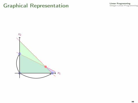
Linear ProgrammingInteger Linear ProgrammingGraphical Representation
?? x1
x2
?? x1
x2
46

Linear ProgrammingInteger Linear ProgrammingGraphical Representation
?? x1
x2
?? x1
x2
46

Linear ProgrammingInteger Linear ProgrammingEfficiency of Simplex Method
I Trying all points is ≈ 4m
I In practice between 2m and 3m iterations
I Clairvoyant’s rule: shortest possible sequence of stepsHirsh conjecture O(n) but best known n1+ln n
49

Linear ProgrammingInteger Linear ProgrammingOutline
1. Linear ProgrammingModeling
Resource AllocationDiet Problem
Solution MethodsGaussian EliminationSimplex Method
2. Integer Linear ProgrammingSolution MethodsApplicationsFinance
50

Linear ProgrammingInteger Linear ProgrammingOutline
1. Linear ProgrammingModeling
Resource AllocationDiet Problem
Solution MethodsGaussian EliminationSimplex Method
2. Integer Linear ProgrammingSolution MethodsApplicationsFinance
51

Linear ProgrammingInteger Linear ProgrammingInteger Linear Programming Problem
max 100x1 + 64x250x1 + 31x2 ≤ 2503x1 − 2x2 ≥ −4
x1, x2 ∈ Z+
LP optimum (376/193, 950/193)IP optimum (5, 0)
x1 + 0.64x2 − 4
3x1 − 2x2 + 4
50x1 + 31x2 − 250
x1
x2
feasible regionconvex but notcontinuous: Now theoptimum can be onthe border (vertices)but also internal.
52

Linear ProgrammingInteger Linear ProgrammingInteger Linear Programming Problem
max 100x1 + 64x250x1 + 31x2 ≤ 2503x1 − 2x2 ≥ −4
x1, x2 ∈ Z+
LP optimum (376/193, 950/193)
IP optimum (5, 0)
x1 + 0.64x2 − 4
3x1 − 2x2 + 4
50x1 + 31x2 − 250
x1
x2
feasible regionconvex but notcontinuous: Now theoptimum can be onthe border (vertices)but also internal.
52

Linear ProgrammingInteger Linear ProgrammingInteger Linear Programming Problem
max 100x1 + 64x250x1 + 31x2 ≤ 2503x1 − 2x2 ≥ −4
x1, x2 ∈ Z+
LP optimum (376/193, 950/193)IP optimum (5, 0)
x1 + 0.64x2 − 4
3x1 − 2x2 + 4
50x1 + 31x2 − 250
x1
x2
feasible regionconvex but notcontinuous: Now theoptimum can be onthe border (vertices)but also internal.
52

Linear ProgrammingInteger Linear ProgrammingCutting Planes
max x1 + 4x2x1 + 6x2 ≤ 18x1 ≤ 3
x1, x2 ≥ 0x1, x2integer
x1 + 6x2 = 18
x1 + 4x2 = 2
x1 = 3
x1 + x2 = 5
x1
x2
53

Linear ProgrammingInteger Linear ProgrammingCutting Planes
max x1 + 4x2x1 + 6x2 ≤ 18x1 ≤ 3
x1, x2 ≥ 0x1, x2integer
x1 + 6x2 = 18
x1 + 4x2 = 2
x1 = 3
x1 + x2 = 5
x1
x2
53

Linear ProgrammingInteger Linear ProgrammingCutting Planes
max x1 + 4x2x1 + 6x2 ≤ 18x1 ≤ 3
x1, x2 ≥ 0x1, x2integer
x1 + 6x2 = 18
x1 + 4x2 = 2
x1 = 3
x1 + x2 = 5
x1
x2
53

Linear ProgrammingInteger Linear ProgrammingCutting Planes
max x1 + 4x2x1 + 6x2 ≤ 18x1 ≤ 3
x1, x2 ≥ 0x1, x2integer
x1 + 6x2 = 18
x1 + 4x2 = 2
x1 = 3
x1 + x2 = 5
x1
x2
53

Linear ProgrammingInteger Linear ProgrammingBranch and Bound
max x1 + 2x2x1 + 4x2 ≤ 84x1 + x2 ≤ 8
x1, x2 ≥ 0, integer
x1 + 4x2 = 8
4x1 + x2 = 8
x1 + 2x2 = 1
x1
x2
54

Linear ProgrammingInteger Linear Programming
4.8x1 ≤ 1 x1 ≥ 2
x1 + 4x2 = 8
4x1 + x2 = 8
x1 + 2x2 = 1
x1 = 1x2
x1
x1 + 4x2 = 8
4x1 + x2 = 8
x1 + 2x2 = 1
x2
x1
55

Linear ProgrammingInteger Linear Programming
4.8−∞
4.5−∞
x1=1x2=1
x2 ≤ 1
x1=0x2=2
x2 ≥ 2
x2 ≤ 1
x1=2x2=0
x1 ≥ 2
x1 + 4x2 = 8
4x1 + x2 = 8
x1 + 2x2 = 1
x2
x1
x1 + 4x2 = 8
4x1 + x2 = 8
x1 + 2x2 = 1
x2
x1
56

Linear ProgrammingInteger Linear Programming
4.8−∞
4.5−∞
33
x1=1x2=1
x2 ≤ 1
44
x1=0x2=2
x2 ≥ 2
x2 ≤ 1
55
x1=2x2=0
x1 ≥ 2
x1 + 4x2 = 8
4x1 + x2 = 8
x1 + 2x2 = 1
x2
x1
x1 + 4x2 = 8
4x1 + x2 = 8
x1 + 2x2 = 1
x2
x1
56

Linear ProgrammingInteger Linear ProgrammingOutline
1. Linear ProgrammingModeling
Resource AllocationDiet Problem
Solution MethodsGaussian EliminationSimplex Method
2. Integer Linear ProgrammingSolution MethodsApplicationsFinance
57

Linear ProgrammingInteger Linear ProgrammingBudget Allocation
(aka, knapsack problem)There is a budget B available for investments in projects during the comingyear and n projects are under consideration, where aj is the cost of project jand cj its expected return.GOAL: chose a set of project such that the budget is not exceeded and theexpected return is maximized.
Variables xj = 1 if project j is selected and xj = 0 otherwise
Objective
maxn∑
j=1
cjxj
Constraints∑nj=1 ajxj ≤ B
xj ∈ {0, 1}∀j = 1, . . . , n
58

Linear ProgrammingInteger Linear ProgrammingFacility Location
Given a certain number of regions, where to install a set of fire stations suchthat all regions are serviced within 8 minutes? For each station the cost ofinstalling the station and which regions it covers are known.
Variables:xj = 1 if the center j is selected and xj = 0 otherwise
Objective:
minn∑
j=1
cjxj
Constraints:∑nj=1 aijxj ≥ 1∀i = 1, . . . ,mxj ∈ {0, 1}∀j = 1, . . . , n
59

Linear ProgrammingInteger Linear ProgrammingOther Applications of MILP
I Energy planning unit commitment(more than 1.000.000 variables of which 300.000integer)
I Scheduling/TimetablingI Examination timetabling/ train timetabling
I Manpower PlanningI Crew Rostering (airline crew, rail crew, nurses)
I RoutingI Vehicle Routing Problem (trucks, planes, trains ...)
60

Linear ProgrammingInteger Linear ProgrammingOutline
1. Linear ProgrammingModeling
Resource AllocationDiet Problem
Solution MethodsGaussian EliminationSimplex Method
2. Integer Linear ProgrammingSolution MethodsApplicationsFinance
61

Linear ProgrammingInteger Linear ProgrammingFinance
In Finance LP can be used:
I By a government to design an optimum tax package to achieve somerequired aim (in particular, an improvement in the balance of payments).
I In revenue management, concerned with setting prices for goods atdifferent times in order to maximize revenue. It is particularly applicableto the hotel, catering, airline and train industries.
I In portfolio selection
62

Linear ProgrammingInteger Linear ProgrammingPortfolio Selection
Given a sum of money to invest, how to spend it among a portfolio of sharesand stocks. The objective is to maintain a certain level of risk and tomaximize the expected rate of return from the investment.
Time
Exc
hang
e in
dex
800
1000
1200
1400
Time
Ass
et p
rices
2040
6080
Time
Ass
et r
etur
ns
0 50 100 150 200 250 300
−0.
8−
0.6
−0.
4−
0.2
0.0
0.2
0.4
cjt A B C1 19.33 8.52 11.842 19.46 9.89 12.283 19.75 9.97 12.344 19.21 9.75 12.125 19.83 10.34 11.846 19.54 9.87 11.947 19.25 10.09 11.698 18.83 9.63 11.569 20.04 9.23 11.6210 19.96 10.43 11.8411 19.75 9.19 12.0012 19.12 9.38 12.4713 18.91 8.92 14.0014 19.79 8.58 14.2515 19.83 9.55 15.03
rjt A B C1 0.01 0.15 0.042 0.01 0.01 0.003 -0.03 -0.02 -0.024 0.03 0.06 -0.025 -0.01 -0.05 0.016 -0.01 0.02 -0.027 -0.02 -0.05 -0.018 0.06 -0.04 0.019 -0.00 0.12 0.0210 -0.01 -0.13 0.0111 -0.03 0.02 0.0412 -0.01 -0.05 0.1213 0.05 -0.04 0.0214 0.00 0.11 0.0515 0.04 0.02 0.12
The trend of the Stock Exchange index (top), and the price (middle) and thereturns (bottom) of three investments.
63

Linear ProgrammingInteger Linear ProgrammingPortfolio Selection - Modeling
Variables: a collection of nonnegative numbers 0 ≤ 0xj ≤ 1, j = 1, . . . ,N thatdivide the capital we want to invest on the stocks j = 1, . . . ,N.
Objective:The return (on each Krone) in the next time period that one would obtainfrom the investment in a portfolio is
R =∑
j
xjRj
and the expected return:
E [R] =∑
j
xjE [Rj ]
We do not know E [Rj ] a good guess is that it is like the average from past
E [Rj ] ≈ R̂j =1T
T∑t=1
rjt
E [R] ≈ R̂ =N∑
j=1
xj R̂j =N∑
j=1
xj1T
T∑t=1
rjt =1T
T∑t=1
N∑j=1
xj rjt
64

Linear ProgrammingInteger Linear ProgrammingPortfolio Selection - Modeling
Variables: a collection of nonnegative numbers 0 ≤ 0xj ≤ 1, j = 1, . . . ,N thatdivide the capital we want to invest on the stocks j = 1, . . . ,N.Objective:The return (on each Krone) in the next time period that one would obtainfrom the investment in a portfolio is
R =∑
j
xjRj
and the expected return:
E [R] =∑
j
xjE [Rj ]
We do not know E [Rj ] a good guess is that it is like the average from past
E [Rj ] ≈ R̂j =1T
T∑t=1
rjt
E [R] ≈ R̂ =N∑
j=1
xj R̂j =N∑
j=1
xj1T
T∑t=1
rjt =1T
T∑t=1
N∑j=1
xj rjt
64

Linear ProgrammingInteger Linear ProgrammingPortfolio Selection - Modeling
Constraints: All and only the capital must used:N∑
j=1
xj = 1
Risk: even though investments are expected to do very well in the long run,they also tend to be erratic in the short term.Many ways to define risk.One way is to define the risk associated with an asset as xj |Rj − E [Rj ]| andthen for the whole portfolio as the mean absolute deviation (MAD):
E[|R − E [R]|
]= E
[∣∣∑j
xj(Rj − E [Rj ])∣∣] ≤ ε
Again, we do not have Rj hence, the estimates for reward E [R] and riskMAD are:
M̂AD =1T
T∑t=1
[∣∣ N∑j=1
xj(rjt − R̂j)∣∣] ≤ ε
65

Linear ProgrammingInteger Linear ProgrammingPortfolio Selection - Final Model
max1T
T∑t=1
N∑j=1
xj rjt
s.t.N∑
j=1
xj = 1
N∑j=1
xj(rjt − R̂j) ≤ ε ∀t = 1..T
N∑j=1
xj(R̂j − rj,t) ≤ ε ∀t = 1..T
0 ≤ xj ≤ 1 ∀j = 1..N
66

Linear ProgrammingInteger Linear ProgrammingPossible Extensions (1)
Due to management costs, at least 10 different assets must be bought.
We need to introduce binary variables zj for each j = 1..N that indicateswhether we are buying or not the asset and then add two constraints to themodel of Task 1:
max1T
T∑t=1
N∑j=1
xj rjt
s.t.(2)− (4)
0 ≤ xj ≤ 1 ∀j = 1..Nzj ≥ xj ∀j = 1..N
N∑j=1
zj ≤ 10
zj ∈ {0, 1} ∀j = 1..N
67

Linear ProgrammingInteger Linear ProgrammingPossible Extensions (1)
Due to management costs, at least 10 different assets must be bought.We need to introduce binary variables zj for each j = 1..N that indicateswhether we are buying or not the asset and then add two constraints to themodel of Task 1:
max1T
T∑t=1
N∑j=1
xj rjt
s.t.(2)− (4)
0 ≤ xj ≤ 1 ∀j = 1..Nzj ≥ xj ∀j = 1..N
N∑j=1
zj ≤ 10
zj ∈ {0, 1} ∀j = 1..N
67

Linear ProgrammingInteger Linear ProgrammingPossible Extensions (2)
Another practical issue due to management costs: the fraction of assets toallocate in one investment can be either zero or a value between 0.02 and 1.
max1T
T∑t=1
N∑j=1
xj rjt
s.t.(2)− (4)
xj ≤ zj ∀j = 1..Nxi ≥ 0.02zj ∀j = 1..N0 ≤ xj ≤ 1 ∀j = 1..Nzj ∈ {0, 1} ∀j = 1..N
68

Linear ProgrammingInteger Linear ProgrammingExample
max 6x1 + 8x25x1 + 10x2 ≤ 604x1 + 4x2 ≤ 40
x1, x2 ≥ 0
x1 x2 x3 x4 −z bx3 5 10 1 0 0 60x4 4 4 0 1 0 40
6 8 0 0 1 0
x3 = 60 − 5x1 − 10x2x4 = 40 − 4x1 − 4x2
z = + 6x1 + 8x2
...
x1 x2 x3 x4 −z bx2 0 1 1/5 −1/4 0 2x1 1 0 −1/5 1/2 0 8
0 0 −2/5 −1 1 −64
x1 = 2 − 1/5x3 + 1/4x4
x2 = 8 + 1/5x3 − 1/2x4
z = 64 − 2/5x3 − 1x4
69

Linear ProgrammingInteger Linear ProgrammingException Handling
1. Unboundedness
2. More than one solution
3. DegeneraciesI benignI cycling
4. Infeasible starting
70

Linear ProgrammingInteger Linear ProgrammingSummary
1. Linear ProgrammingModeling
Resource AllocationDiet Problem
Solution MethodsGaussian EliminationSimplex Method
2. Integer Linear ProgrammingSolution MethodsApplicationsFinance
A nice talk on planning at DSB-S http://www.dr.dk/DR2/Danskernes+akademi/IT_teknik/Saet_dog_et_andet_tog_ind.htm
71