Slides from Advanced Tutorial WSC 09

Department of Industrial Engineering and Management Sciences

Better Simulation Metamodeling:The Why, What and How

of Stochastic Kriging

Jeremy StaumCollaborators:

Bruce Ankenman, Barry Nelson Evren Baysal, Ming Liu, Wei Xie

supported by the NSF under Grant No. DMI-0900354


Outline• overview of metamodeling• metamodeling approaches

• regression, kriging, stochastic kriging• Why kriging? Why stochastic kriging?• stochastic kriging: what and how• practical advice for stochastic kriging


Metamodeling: Why?• simulation model

• input x, response surface y(x) • simulation effort n• simulation output Y(x;n) estimates y(x)• Y(x;n) converges to y(x) as n→∞

• simulation metamodeling• fast estimate of y(x) for any x• “What would the simulation say if I ran it?”


Uses of Metamodeling• trend modeling (global)

• Does y(x) = y(x1,x2) increase with x1?• Is y(x) = y(x1,x2) more sensitive to x1 or x2?• y(x) is similar to β0 + xβ globally

• optimization (local)• Which way to move and how far?• quadratic: first and second derivatives,

y(x) ≈ β0 + xβ + xTQx locally


Uses of Metamodeling• exploration• (global)• What if?

scenario = x• multi-objective

tradeoffs• throughput (x1)• cycle time (y)


Uses of Metamodeling• scenario analysis

• (global)• can’t control scenario• financial scenario• military scenario• simulation inputs

• probabilistic analysis• distribution on scenarios


Needs of Metamodeling• trend modeling: rough global trend• optimization: rough local trend• exploration / scenario analysis:

• globally accurate prediction: ŷ(x) ≈ y(x)• ŷ(x) is almost as good an estimator of y(x)

as the simulation output Y(x;n)• but metamodel is much faster than model• “simulation on demand”


Overview of Approaches• No free lunch!• Inference about y(x) without seeing

Y(x;n) requires assumptions: • about spatial variability in y(·)• about noise ε(x;n) = Y(x;n) – y(x)

• Is y(·) a simple trend y(x)=b(x)β, or must we model deviation from trend?

• Should we try to filter out noise?


Regression• Assume y(x) = b(x)β.

• The truth y can’t deviate from the trend.• We aim only to estimate β.

• Assume ε(x) = Y(x) – y(x) is white noise.• Aim to filter it out!• Var[ε(x)] doesn’t depend on x. (remedies)

• Global metamodeling: can’t find an adequate trend model (b).


Interpolation• Assume y(·) has some smoothness.

• model mean β0 and deviation y(·) - β0 or• trend b(·)β and deviation y(·) - b(·)β

• Assume ε(x) = Y(x) – y(x) = 0.• No filtering: ŷ(x) = Y(x) if x is simulated.

• Stochastic simulation: need big simulation effort n so Y(x;n) – y(x) ≈ 0.• Interpolated ŷ(·) will look bumpy.


Smoothing• Assume y(·) has some smoothness.

• just like interpolation • Assume ε(x) = Y(x) – y(x) is white noise.

• Aim to filter it out!• Can handle ordinal & categorical data.

• regression, interpolation, or smoothing


Example: M/M/1 Queue• arrival rate 1• service rate x• steady-state mean wait y(x)=1/(x(x-1))• initialize in steady-state (no bias) and

simulate a fixed # of customers• variance also explodes as x↓1


Regression Remedies• weighted least squares (WLS)

• weight on Y(x;n) is n/Var[Y(x)]• empirical WLS: estimate Var[Y(x)]

• generalized linear models:• Y(x) = y(x) + ε(x), y(x) = LINK(b(x)β)• perfect for M/M/1: y(x) =

exp(β0 + β1ln(x) + β2ln(x-1)) = 1/(x(x-1))


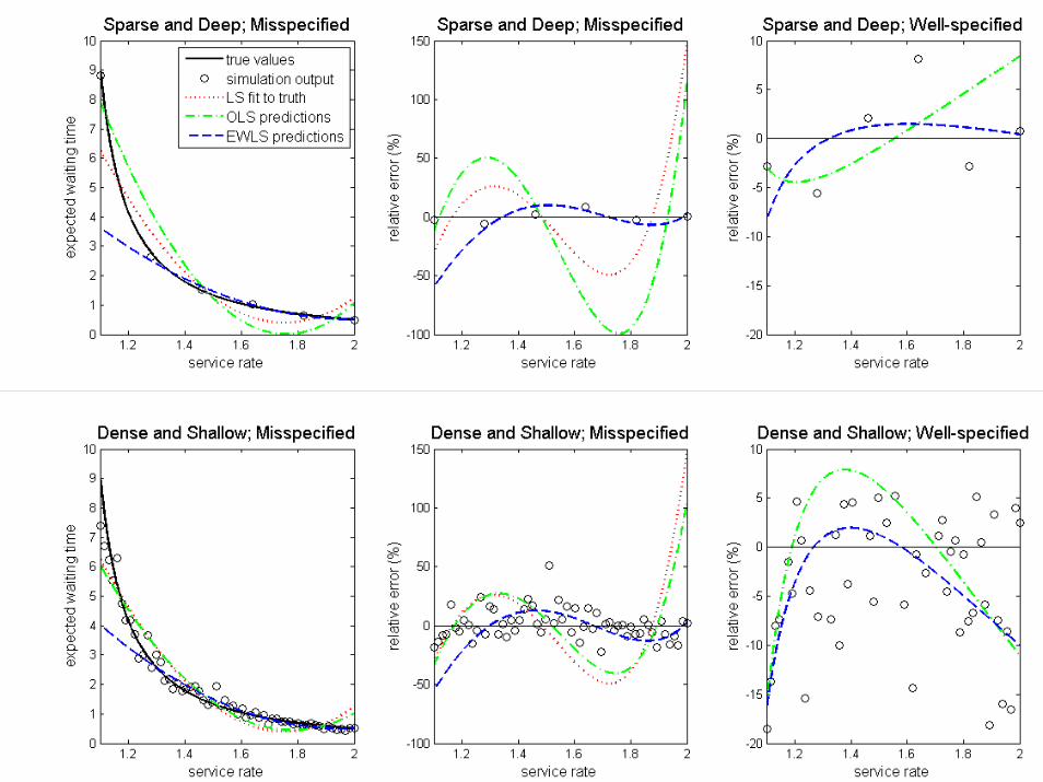
Experiment Design• M/M/1: one-dimensional, evenly spaced• k design points: x1=1.1, …, xk=2• constant simulation effort n at each

• 30 replications = runs of n customers each• Var[Y(x;n)] is huge for x=1.1, small for x=2

• Two experiment designs:• sparse & deep: k=6, n=1000 customers• dense & shallow: k=60, n=100 customers


Regression: Conclusions• misspecification → poor predictions

• the WHY of interpolation (including kriging) • weighted least squares: dangerous!

• WLS assumes a well-specified model • assigns huge residuals to high-variance

observations, predicts very badly there• Want a well-specified model?

• good luck, hard work


Interpolation• Deviations from trend are meaningful.• Can omit trend modeling (overall mean).• prediction ŷ(x) at x after simulating at

design points x1, …, xk:• if x = xi is simulated, ŷ(xi) = Y(xi)• if not, ŷ(x) = w1Y(x1) + … + wkY(xk) where

wi is larger for xi closer to x


Kriging: Spatial Corr.• deterministic simulation:

• ε(x) = Y(x) – y(x) = 0.• Y(·) is regarded as a random field

• each Y(x) is a random variable (Bayesian)• Corr[Y(x),Y(x’)] = r(x-x’)

• e.g. r(x-x’) = exp(-∑i θi|xi – x’i|)• or r(x-x’) = exp(-∑i θi (xi – x’i)2)


Kriging Prediction• prior: Y(·) is a Gaussian random field

• E[Y(x)] = b(x)β, often = β0

• Cov[Y(x),Y(x’)] = τ2r(x-x’)• observe Y = (Y(x1), …, Y(xk))• posterior mean:

• ŷ(x) = b(x)β + r(x) R-1 (Y – Bβ)• ri(x) = r(x-xi), Rij = r(xj-xi), Bi· = b(xi)


Choices in Kriging• basis functions b(·) for trend b(x)β

• estimate coefficients β by least-squares: min ∑i (Y(xi) - b(x)β)2

• spatial correlation function r(·;θ)• estimate coefficients θ by cross-validation

or maximizing likelihood of Y(x1), …, Y(xk)• axis transformation affects predictions

• arrival & service rates vs. arrival rate, load


Pathologies of Kriging• reversion to the trend• fitting to noise→WHY stochastic kriging


Kriging with Errors• measurement error or nugget effect

• ε(x) = Y(x) – y(x) ≠ 0• filter out noise that harms prediction• improve numerical stability

• intrinsic vs. extrinsic uncertainty• intrinsic: Var[ε(x)] from physical experiment

or noise from stochastic simulation• extrinsic: Var[Y(x)] representing our

ignorance


How to Apply Krigingto Stochastic Simulation• Kleijnen & van Beers

• control noise and its effect on prediction• Siem & den Hertog

• reduce sensitivity to stochastic noise• Yin, Ng & Ng: modified nugget effect• Ankenman, Nelson & Staum

• stochastic kriging


Stochastic Kriging• Intrinsic uncertainty ε(x) = Y(x) – y(x)

is independent of extrinsic uncertainty.• If simulation effort n at x is large,

ε(x;n) = Y(x;n) – y(x)• is approximately normal • we can estimate its variance v(x)/n• do empirical weighted least squares


The “What” of SK• The kriging prediction

• ŷ(x) = b(x)β + r(x) R-1 (Y – Bβ) where• ri(x) = r(x-xi), Rij = r(xj-xi), Bi· = b(xi)

• The stochastic kriging prediction• ŷ(x) = b(x)β + r(x) (R+C/τ2)-1 (Y – Bβ)• C = intrinsic covariance matrix• τ2 = extrinsic variance

• Awareness of noise alters inference.


Behavior of SK• If sampling is independent, diagonal C:

• Cii = intrinsic noise in observing Y(xi)• The signal-to-noise ratio Cii/τ2 governs

smoothing: how far ŷ(xi) is from y(xi).• Extreme cases:

• C ↓ 0: SK → kriging• τ2 ↓ 0: SK → EWLS regression

• neglecting Y(xi) if Cii >> τ2!


Examples• M/M/1 Queue

• high intrinsic variance for low service rate x• a simulated game

• A tosses a coin, heads with prob. x• B tosses another, heads with prob. 1-x• HT → B pays A $1; TH → A pays B $1• y(x) = 2x-1• intrinsic variance v(x) highest in the middle


SK: How-To Overview• pre-simulation:

• choose axes and correlation function r• choose design points and effort: xi, ni

• simulate: for each i=1, …, k,• observe Y(xi), estimate variance v(xi)

• post-simulation:• estimate parameters β, θ, τ2

• predict ŷ(x) for any x desired


Multi-Product Cycle Time• simulate Jackson network with 3 nodes• input x has 3 dimensions: (did up to 8)

• mix of 3 products (ranging from 0%-100%)• load on bottleneck node (from 0.6-0.8)

• 201 design points (low-discrepancy)• reduce heteroscedasticity by planning

run lengths via approximation• intrinsic std. error still varied over 10-fold


0 0.1 0.2 0.3 0.4 0.5 0.6 0.7 0.8 0.9 1

5

6

7

8

9

10

alpha1

CTα2:α3 = 1:6, x = 0.65 (gauss function)

fitted curve for prod 1)fitted curve for prod 2)

fitted curve for prod 3)

true values of product 1

true values of product 2true values of product 3


SK: Practical Advice• Use the Gaussian correlation function

• r(x-x’) = exp(-∑i θi (xi – x’i)2) • for smoothness of random field, need

r(x-x’) → 1 slowly as x-x’ → 0• misspecification: spatial homogeneity

• spatial transformation• trend modeling?


SK: Practical Advice• Don’t extrapolate! Beware edge effect.

• bias due to one-sided smoothing near edge

• Placement of design points is important.• Grids are not good in high dimension.• The goal is not the same as in regression.• For uniformity: low-discrepancy sequences.

• Kriging can use lots of CPU time, memory for >1000 design points.


SK: Practical Advice• Make intrinsic variance Var[Y(xi)]/ni

smaller than variability of Y(x1), …, Y(xk)• or of Y(x1)-b(x1)β, …, Y(xk)-b(xk)β• Can use two-stage procedure to control

intrinsic variance.• More design points are better than very

low variance at a few points.• Big k, but avoid excessive noise or cost.


SK: Posterior Variance• Prediction is posterior mean:

• ŷ(x) = b(x)β + r(x) (R+C/τ2)-1 (Y – Bβ)• Posterior variance:

• τ2(1 – r(x) (R+C/τ2)-1 r(x)T)• Don’t trust posterior variance!

• misleading due to misspecification of GRF• can guide effort in multi-stage procedures• Kleijnen: bootstrapping & cross-validation


SK: Amelioration• Spatial inhomogeneity: better-specified

• data-driven spatial transformation• non-stationary covariance functions• partitioning: “treed” GRFs

• Computational cost:• r(x-x’)=0 if x’ far from x; sparse matrices• covariance tapering: set small corr to 0


Conclusions• Global metamodeling may be feasible.

• harnessing computer idle time• Consider stochastic kriging when:

• regression isn’t enough• computational budget is limited• fewer than 1000 design points (for now)

• www.stochastickriging.net• papers, MATLAB code

http://www.stochastickriging.net/

Slides from Advanced Tutorial WSC 09

Documents

Transcript of Slides from Advanced Tutorial WSC 09