
Slide 8- 1. Chapter 8 SQL: SchemaDefinition, Constraints, and Queries and Views.
71
Slide 8- 1
-
Upload
lillian-hunter -
Category
Documents
-
view
221 -
download
0
Transcript of Slide 8- 1. Chapter 8 SQL: SchemaDefinition, Constraints, and Queries and Views.
Slide 8- 1
Chapter 8
SQL: SchemaDefinition, Constraints, and Queries and Views
Slide 8- 3
History of SQL
SQL: Structured Query Language
In 1974, D. Chamberlin (IBM San Jose Laboratory) defined language called ‘Structured English Query Language’ (SEQUEL).
A revised version, SEQUEL/2, was defined in 1976 but name was subsequently changed to SQL for legal reasons.
Slide 8- 4
History of SQL
Still pronounced ‘see-quel’, though official pronunciation is ‘S-Q-L’.
IBM subsequently produced a prototype DBMS called System R, based on SEQUEL/2.
Slide 8- 5
History of SQL
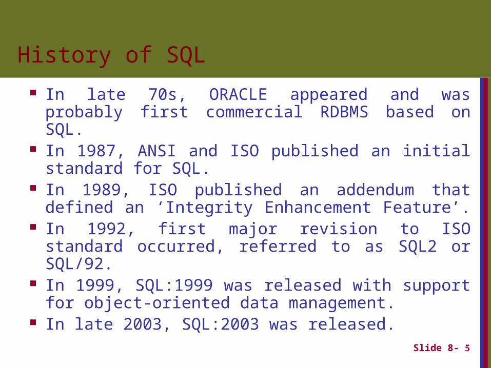
In late 70s, ORACLE appeared and was probably first commercial RDBMS based on SQL.
In 1987, ANSI and ISO published an initial standard for SQL.
In 1989, ISO published an addendum that defined an ‘Integrity Enhancement Feature’.
In 1992, first major revision to ISO standard occurred, referred to as SQL2 or SQL/92.
In 1999, SQL:1999 was released with support for object-oriented data management.
In late 2003, SQL:2003 was released.
Slide 2- 6
DBMS Languages
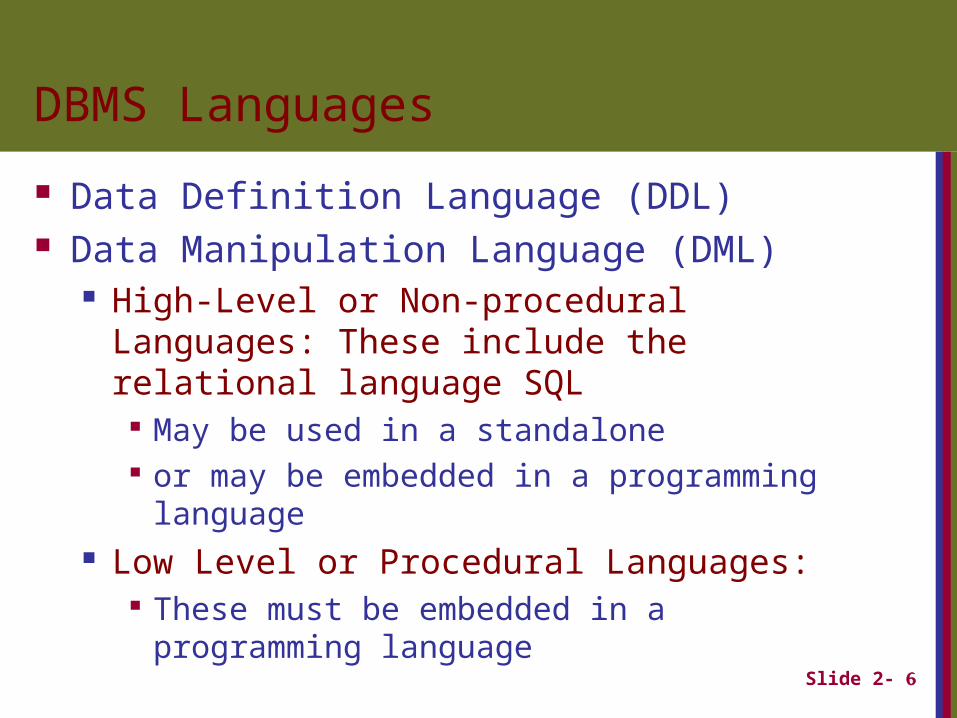
Data Definition Language (DDL) Data Manipulation Language (DML)
High-Level or Non-procedural Languages: These include the relational language SQL
May be used in a standalone or may be embedded in a programming language
Low Level or Procedural Languages: These must be embedded in a programming
language
Slide 2- 7
DBMS Languages
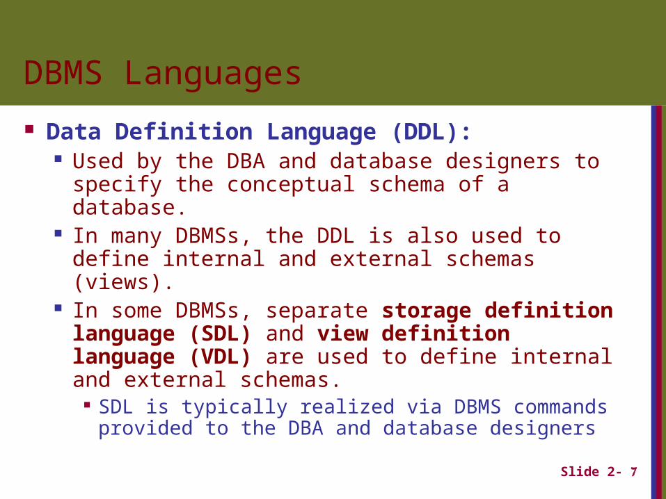
Data Definition Language (DDL): Used by the DBA and database designers to
specify the conceptual schema of a database. In many DBMSs, the DDL is also used to define
internal and external schemas (views). In some DBMSs, separate storage definition
language (SDL) and view definition language (VDL) are used to define internal and external schemas.
SDL is typically realized via DBMS commands provided to the DBA and database designers
Slide 2- 8
DBMS Languages
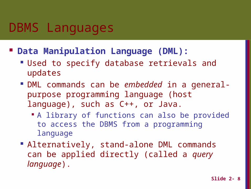
Data Manipulation Language (DML): Used to specify database retrievals and updates DML commands can be embedded in a general-
purpose programming language (host language), such as C++, or Java.
A library of functions can also be provided to access the DBMS from a programming language
Alternatively, stand-alone DML commands can be applied directly (called a query language).
Slide 2- 9
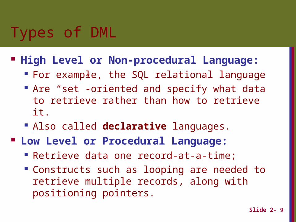
Types of DML
High Level or Non-procedural Language: For example, the SQL relational language Are “set”-oriented and specify what data to retrieve
rather than how to retrieve it. Also called declarative languages.
Low Level or Procedural Language: Retrieve data one record-at-a-time; Constructs such as looping are needed to retrieve
multiple records, along with positioning pointers.
Slide 8- 10
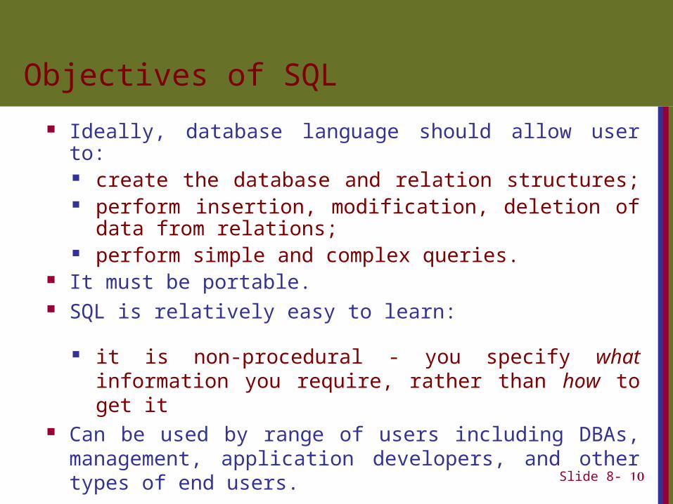
Objectives of SQL
Ideally, database language should allow user to: create the database and relation structures; perform insertion, modification, deletion of data from
relations; perform simple and complex queries.
It must be portable. SQL is relatively easy to learn:
it is non-procedural - you specify what information you require, rather than how to get it
Can be used by range of users including DBAs, management, application developers, and other types of end users.
Slide 8- 11
Objectives of SQL
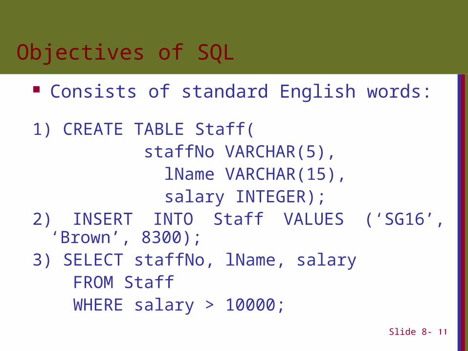
Consists of standard English words:
1) CREATE TABLE Staff(staffNo VARCHAR(5),
lName VARCHAR(15), salary INTEGER);
2) INSERT INTO Staff VALUES (‘SG16’, ‘Brown’, 8300);
3) SELECT staffNo, lName, salary FROM Staff WHERE salary > 10000;
Slide 8- 12
Writing SQL Commands
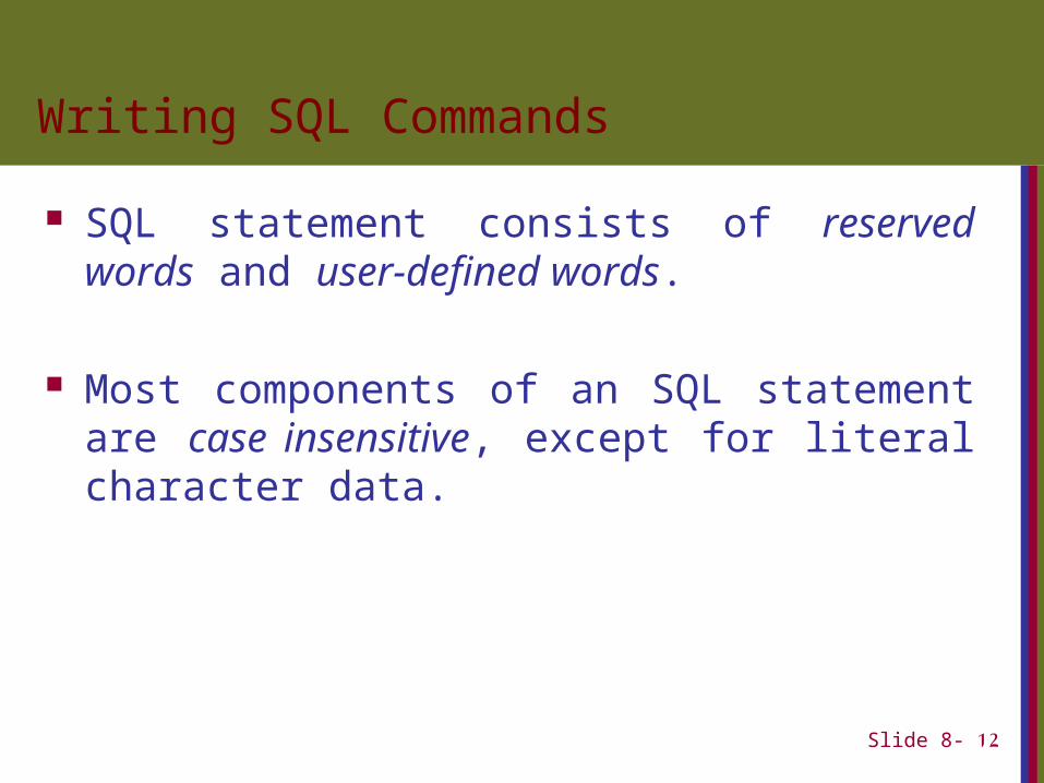
SQL statement consists of reserved words and user-defined words.
Most components of an SQL statement are case insensitive, except for literal character data.
Slide 8- 13
Writing SQL Commands
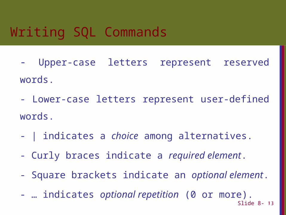
- Upper-case letters represent reserved words.
- Lower-case letters represent user-defined words.
- | indicates a choice among alternatives.
- Curly braces indicate a required element.
- Square brackets indicate an optional element.
- … indicates optional repetition (0 or more).
Slide 8- 14
Literals
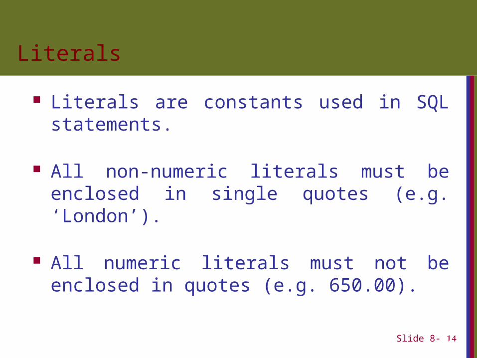
Literals are constants used in SQL statements.
All non-numeric literals must be enclosed in single quotes (e.g. ‘London’).
All numeric literals must not be enclosed in quotes (e.g. 650.00).
Attribute Data Types in SQL
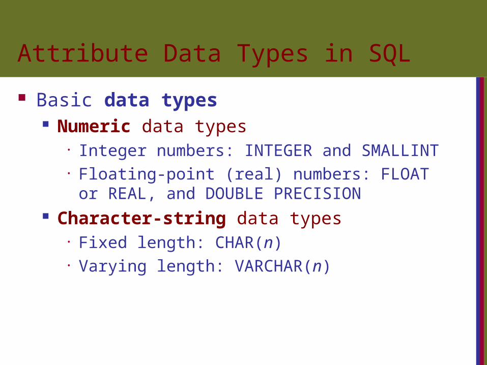
Basic data types Numeric data types
• Integer numbers: INTEGER and SMALLINT• Floating-point (real) numbers: FLOAT or REAL, and DOUBLE PRECISION
Character-string data types • Fixed length: CHAR(n)• Varying length: VARCHAR(n)
Attribute Data Types in SQL (cont’d.)
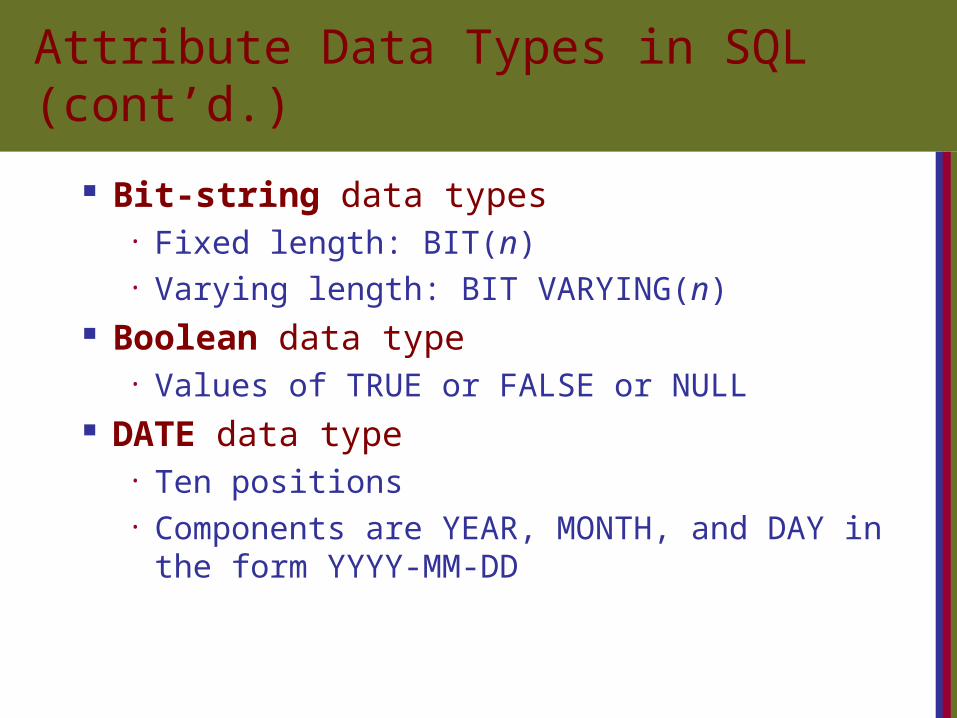
Bit-string data types • Fixed length: BIT(n)• Varying length: BIT VARYING(n)
Boolean data type • Values of TRUE or FALSE or NULL
DATE data type • Ten positions• Components are YEAR, MONTH, and DAY in the
form YYYY-MM-DD
Attribute Data Types in SQL (cont’d.)
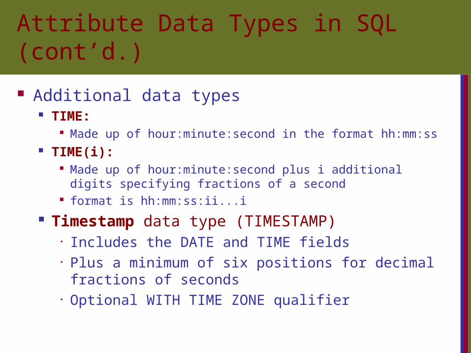
Additional data types TIME:
Made up of hour:minute:second in the format hh:mm:ss TIME(i):
Made up of hour:minute:second plus i additional digits specifying fractions of a second
format is hh:mm:ss:ii...i
Timestamp data type (TIMESTAMP)• Includes the DATE and TIME fields• Plus a minimum of six positions for decimal fractions
of seconds• Optional WITH TIME ZONE qualifier
Attribute Data Types in SQL (cont’d.)
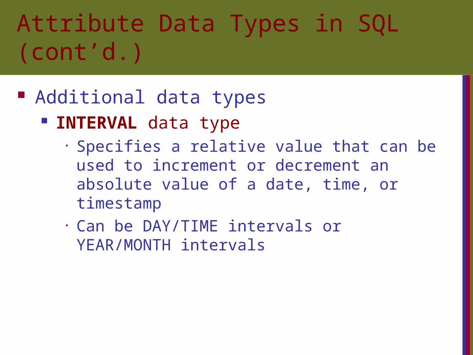
Additional data types INTERVAL data type
• Specifies a relative value that can be used to increment or decrement an absolute value of a date, time, or timestamp
• Can be DAY/TIME intervals or YEAR/MONTH intervals
Slide 8- 19
Data Definition, Constraints, and Schema Changes
Used to CREATE, DROP, and ALTER the descriptions of the tables (relations) of a database
Slide 8- 20
CREATE TABLE
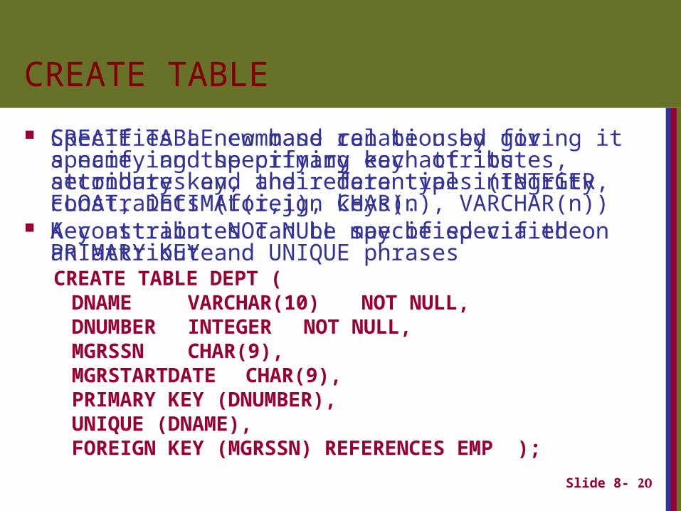
CREATE TABLE DEPT (DNAME VARCHAR(10) NOT NULL,DNUMBER INTEGER NOT NULL,MGRSSN CHAR(9),MGRSTARTDATE CHAR(9),PRIMARY KEY (DNUMBER),UNIQUE (DNAME),FOREIGN KEY (MGRSSN) REFERENCES EMP );
CREATE TABLE command can be used for specifying the primary key attributes, secondary key, and referential integrity constraints (foreign keys).
Key attributes can be specified via the PRIMARY KEY and UNIQUE phrases
Specifies a new base relation by giving it a name, and specifying each of its attributes and their data types (INTEGER, FLOAT, DECIMAL(i,j), CHAR(n), VARCHAR(n))
A constraint NOT NULL may be specified on an attribute
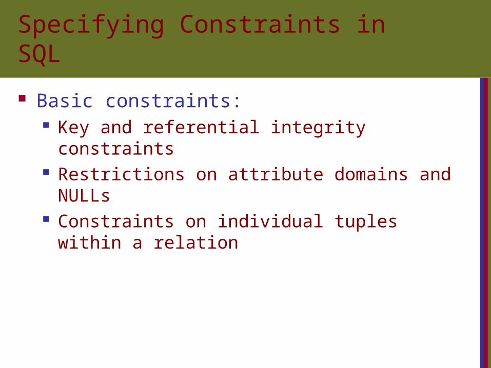
Specifying Constraints in SQL
Basic constraints: Key and referential integrity constraints Restrictions on attribute domains and NULLs Constraints on individual tuples within a relation
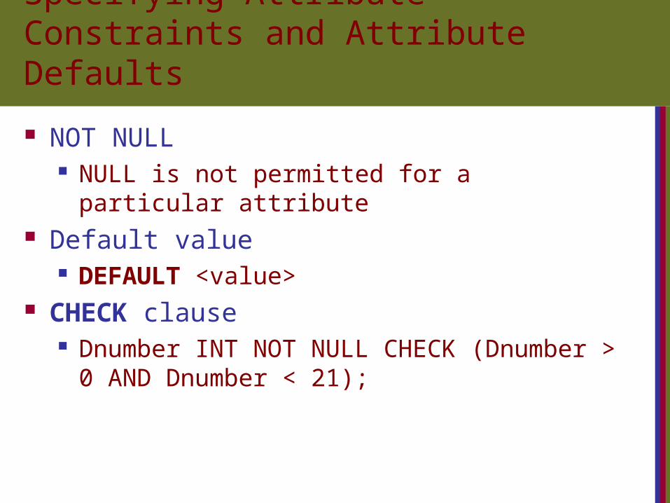
Specifying Attribute Constraints and Attribute Defaults
NOT NULL NULL is not permitted for a particular attribute
Default value DEFAULT <value>
CHECK clause Dnumber INT NOT NULL CHECK (Dnumber > 0 AND Dnumber < 21);
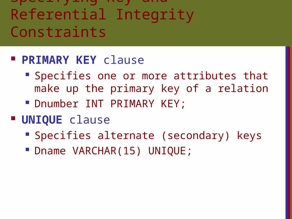
Specifying Key and Referential Integrity Constraints
PRIMARY KEY clause Specifies one or more attributes that make up the
primary key of a relation Dnumber INT PRIMARY KEY;
UNIQUE clause Specifies alternate (secondary) keys Dname VARCHAR(15) UNIQUE;
Specifying Key and Referential Integrity Constraints (cont’d.)
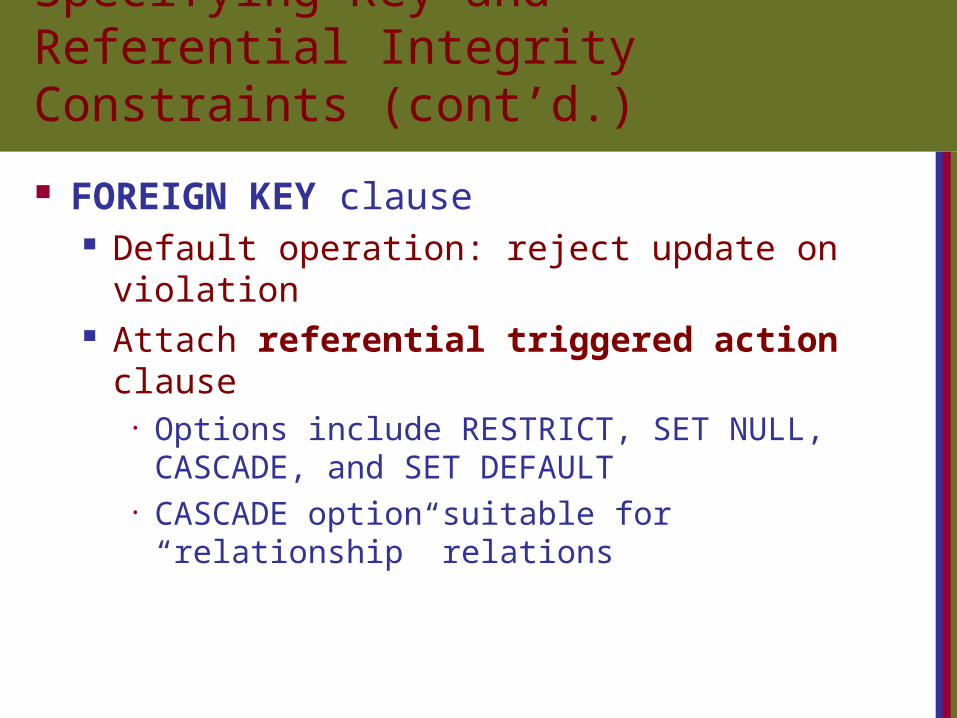
FOREIGN KEY clause Default operation: reject update on violation Attach referential triggered action clause
• Options include RESTRICT, SET NULL, CASCADE, and SET DEFAULT
• CASCADE option suitable for “relationship” relations
Slide 8- 26
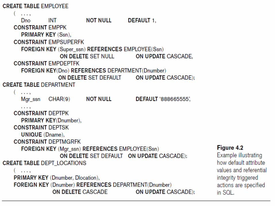
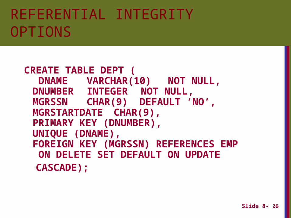
REFERENTIAL INTEGRITY OPTIONS
CREATE TABLE DEPT ( DNAME VARCHAR(10) NOT NULL,DNUMBER INTEGER NOT NULL,MGRSSN CHAR(9) DEFAULT ‘NO’,MGRSTARTDATE CHAR(9),PRIMARY KEY (DNUMBER),UNIQUE (DNAME),FOREIGN KEY (MGRSSN) REFERENCES EMP ON DELETE SET DEFAULT ON UPDATE
CASCADE);
Slide 8- 27
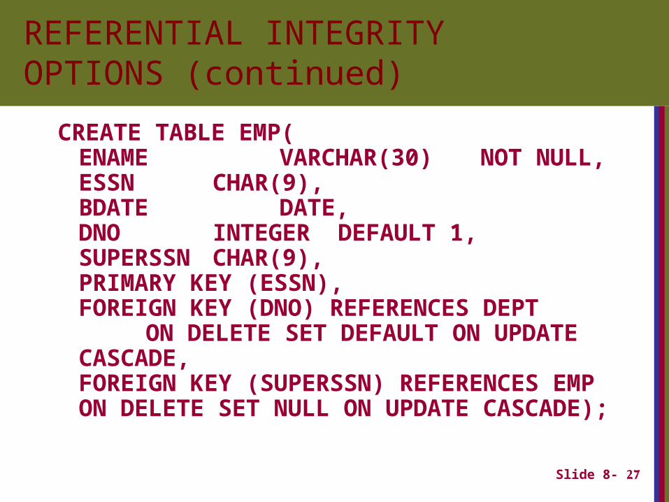
REFERENTIAL INTEGRITY OPTIONS (continued)
CREATE TABLE EMP(ENAME VARCHAR(30) NOT NULL,ESSN CHAR(9),BDATE DATE,DNO INTEGER DEFAULT 1,SUPERSSN CHAR(9),PRIMARY KEY (ESSN),FOREIGN KEY (DNO) REFERENCES DEPT
ON DELETE SET DEFAULT ON UPDATE CASCADE,FOREIGN KEY (SUPERSSN) REFERENCES EMP ON DELETE SET NULL ON UPDATE CASCADE);
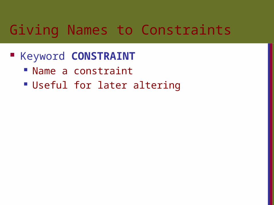
Giving Names to Constraints
Keyword CONSTRAINT Name a constraint Useful for later altering
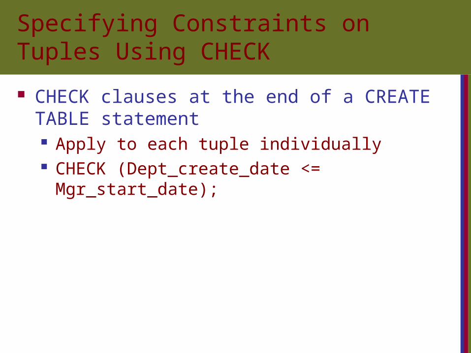
Specifying Constraints on Tuples Using CHECK
CHECK clauses at the end of a CREATE TABLE statement Apply to each tuple individually CHECK (Dept_create_date <= Mgr_start_date);
Slide 8- 30
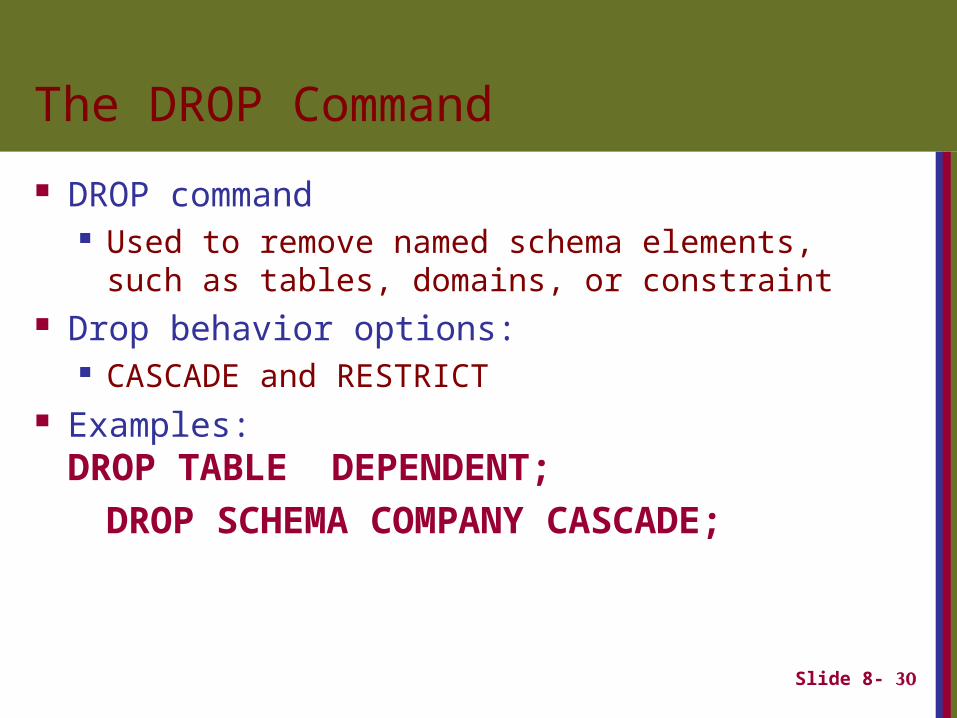
The DROP Command
DROP command Used to remove named schema elements, such as
tables, domains, or constraint Drop behavior options:
CASCADE and RESTRICT Examples:DROP TABLE DEPENDENT;
DROP SCHEMA COMPANY CASCADE;
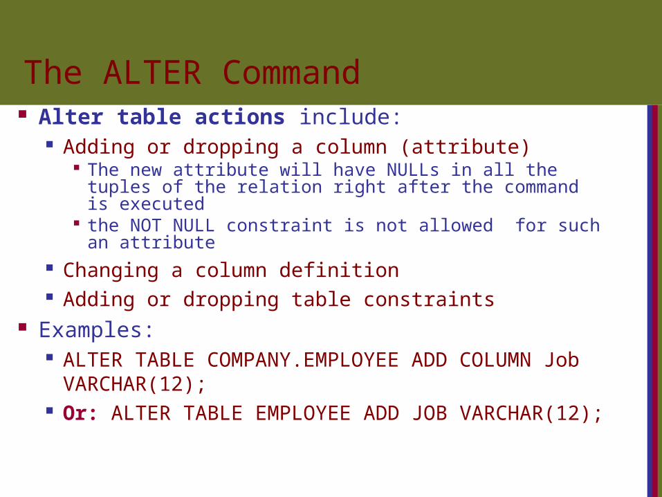
The ALTER Command Alter table actions include:
Adding or dropping a column (attribute) The new attribute will have NULLs in all the tuples of the
relation right after the command is executed the NOT NULL constraint is not allowed for such an attribute
Changing a column definition Adding or dropping table constraints
Examples: ALTER TABLE COMPANY.EMPLOYEE ADD COLUMN Job VARCHAR(12);
Or: ALTER TABLE EMPLOYEE ADD JOB VARCHAR(12);

The ALTER Command (cont’d.)
The database users must still enter a value for the new attribute JOB for each EMPLOYEE tuple. This can be done using the UPDATE command.
To drop a column Choose either CASCADE or RESTRICT
Change constraints specified on a table Add or drop a named constraint
Slide 8- 33
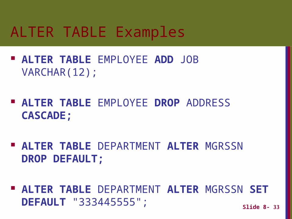
ALTER TABLE Examples
ALTER TABLE EMPLOYEE ADD JOB VARCHAR(12);
ALTER TABLE EMPLOYEE DROP ADDRESS CASCADE;
ALTER TABLE DEPARTMENT ALTER MGRSSN DROP DEFAULT;
ALTER TABLE DEPARTMENT ALTER MGRSSN SET DEFAULT "333445555";

Slide 8- 34
Slide 8- 35
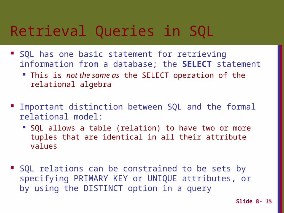
Retrieval Queries in SQL SQL has one basic statement for retrieving information
from a database; the SELECT statement This is not the same as the SELECT operation of the
relational algebra
Important distinction between SQL and the formal relational model:
SQL allows a table (relation) to have two or more tuples that are identical in all their attribute values
SQL relations can be constrained to be sets by specifying PRIMARY KEY or UNIQUE attributes, or by using the DISTINCT option in a query
Slide 8- 36
Retrieval Queries in SQL (contd.)
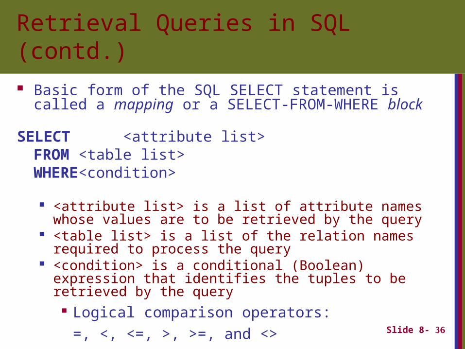
Basic form of the SQL SELECT statement is called a mapping or a SELECT-FROM-WHERE block
SELECT <attribute list>FROM <table list>WHERE <condition>
<attribute list> is a list of attribute names whose values are to be retrieved by the query
<table list> is a list of the relation names required to process the query
<condition> is a conditional (Boolean) expression that identifies the tuples to be retrieved by the query
Logical comparison operators:
=, <, <=, >, >=, and <>
Slide 8- 37
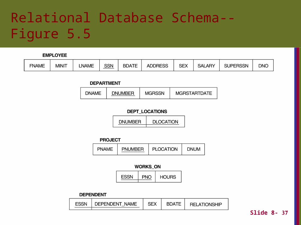
Relational Database Schema--Figure 5.5
Slide 8- 38
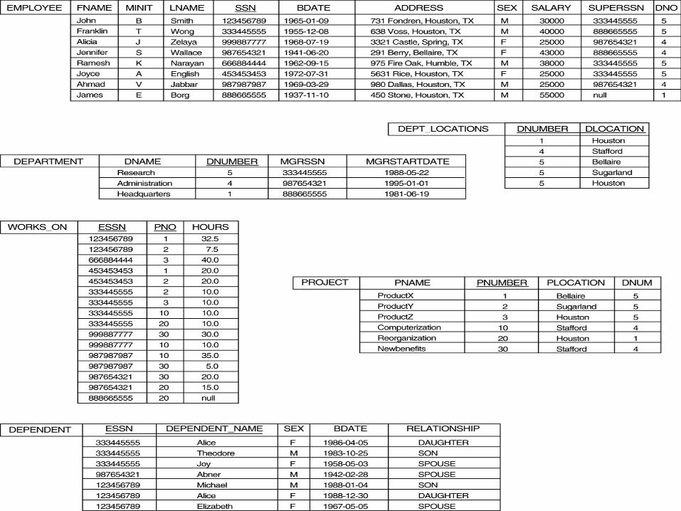
Populated Database--Fig.5.6
Slide 8- 39
Simple SQL Queries
Basic SQL queries correspond to using the following operations of the relational algebra: SELECT PROJECT JOIN
All subsequent examples use the COMPANY database
Slide 8- 41
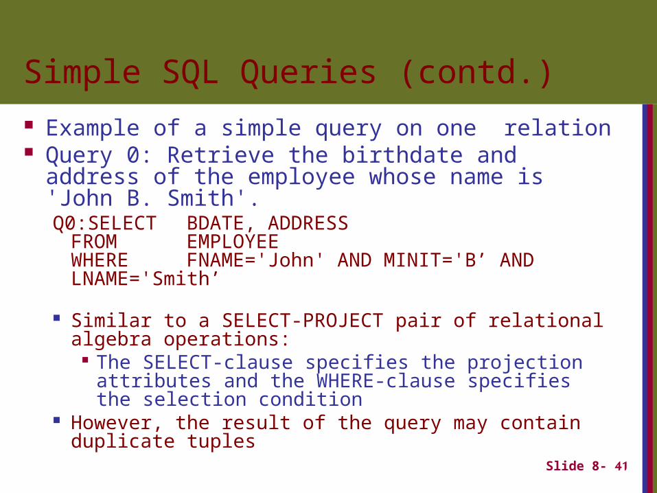
Simple SQL Queries (contd.)
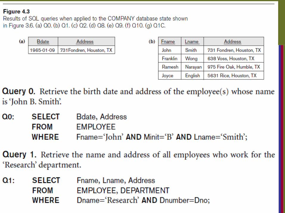
Example of a simple query on one relation Query 0: Retrieve the birthdate and address of
the employee whose name is 'John B. Smith'.Q0:SELECT BDATE, ADDRESS
FROM EMPLOYEEWHERE FNAME='John' AND MINIT='B’
AND LNAME='Smith’
Similar to a SELECT-PROJECT pair of relational algebra operations:
The SELECT-clause specifies the projection attributes and the WHERE-clause specifies the selection condition
However, the result of the query may contain duplicate tuples
Slide 8- 42
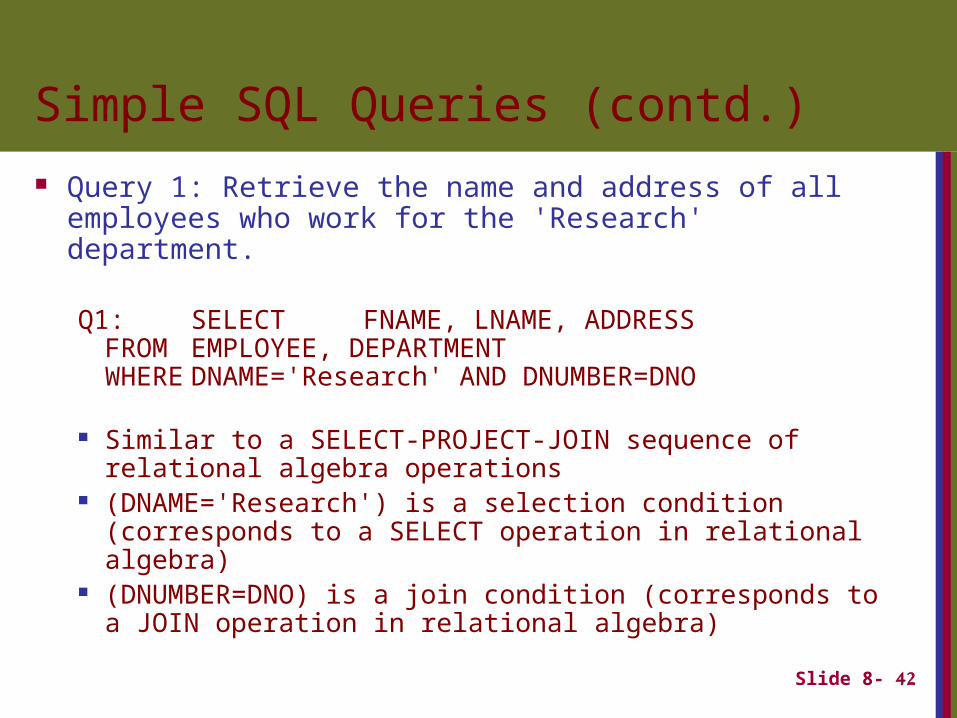
Simple SQL Queries (contd.)
Query 1: Retrieve the name and address of all employees who work for the 'Research' department.
Q1: SELECT FNAME, LNAME, ADDRESSFROM EMPLOYEE, DEPARTMENTWHERE DNAME='Research' AND
DNUMBER=DNO
Similar to a SELECT-PROJECT-JOIN sequence of relational algebra operations
(DNAME='Research') is a selection condition (corresponds to a SELECT operation in relational algebra)
(DNUMBER=DNO) is a join condition (corresponds to a JOIN operation in relational algebra)
Slide 8- 44
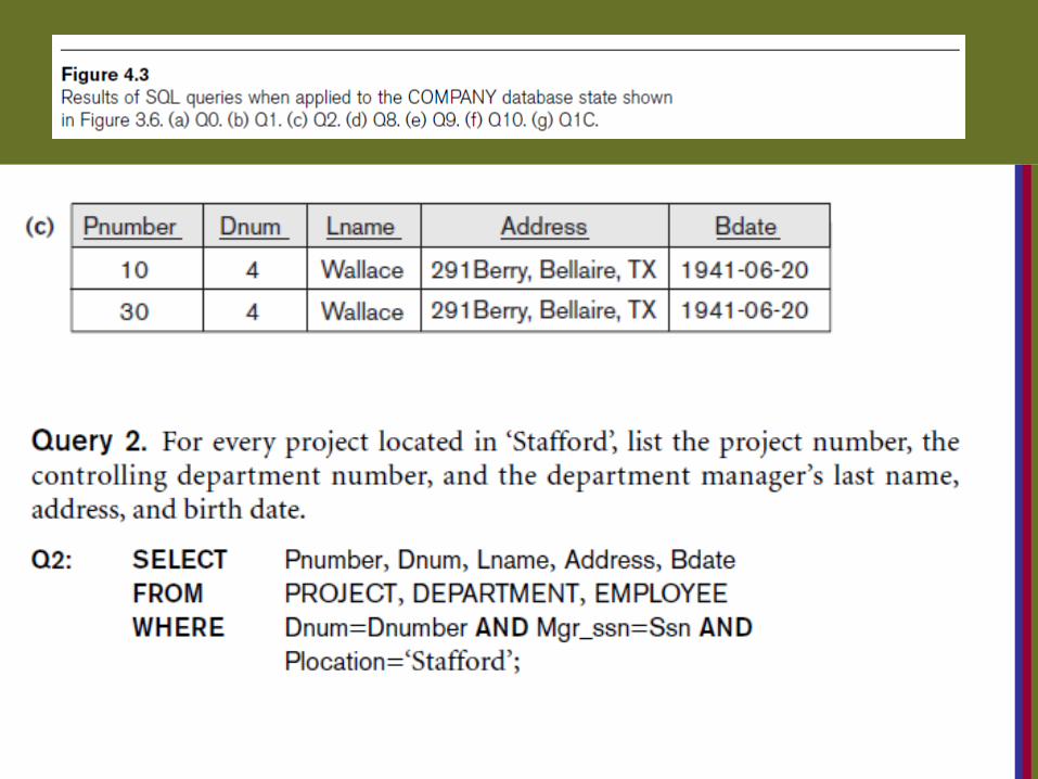
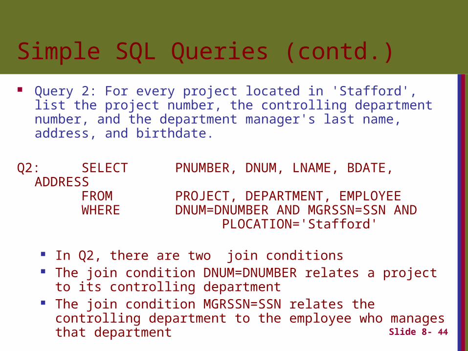
Simple SQL Queries (contd.)
Query 2: For every project located in 'Stafford', list the project number, the controlling department number, and the department manager's last name, address, and birthdate.
Q2: SELECT PNUMBER, DNUM, LNAME, BDATE, ADDRESS
FROM PROJECT, DEPARTMENT, EMPLOYEEWHERE DNUM=DNUMBER AND MGRSSN=SSN AND
PLOCATION='Stafford'
In Q2, there are two join conditions The join condition DNUM=DNUMBER relates a project to its
controlling department The join condition MGRSSN=SSN relates the controlling department
to the employee who manages that department
Slide 8- 45
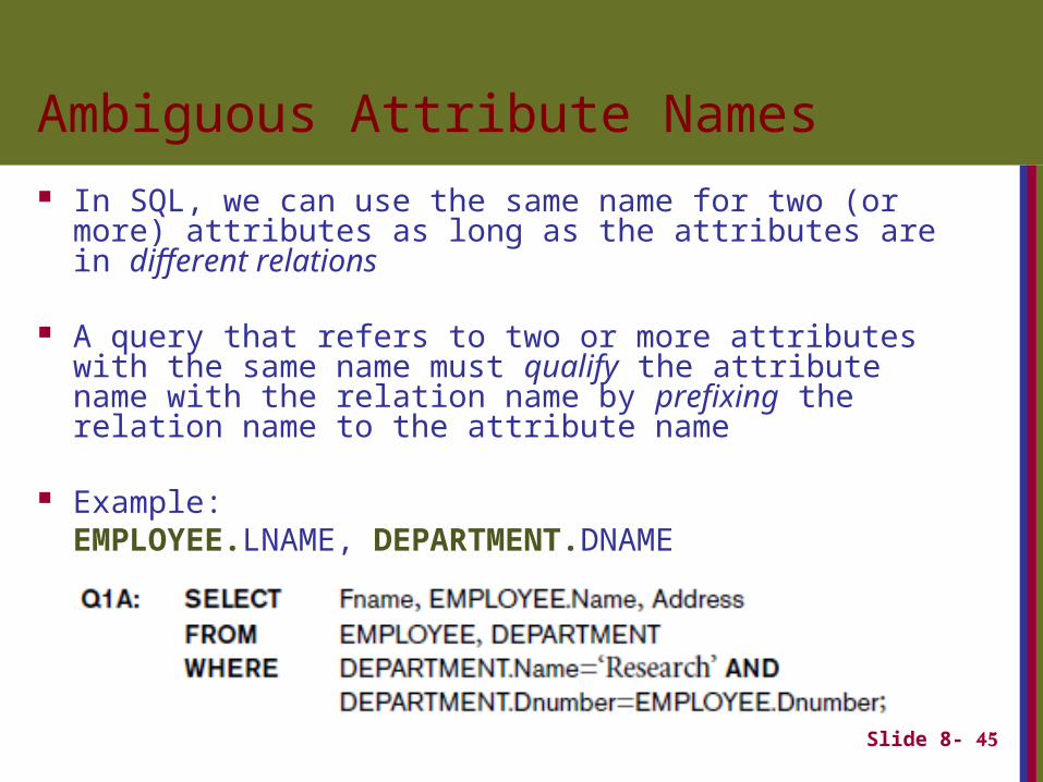
Ambiguous Attribute Names
In SQL, we can use the same name for two (or more) attributes as long as the attributes are in different relations
A query that refers to two or more attributes with the same name must qualify the attribute name with the relation name by prefixing the relation name to the attribute name
Example: EMPLOYEE.LNAME, DEPARTMENT.DNAME
Slide 8- 46
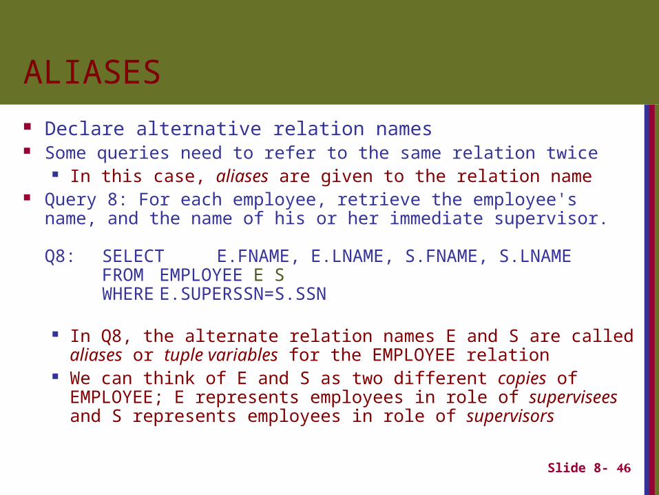
ALIASES
Declare alternative relation names Some queries need to refer to the same relation twice
In this case, aliases are given to the relation name Query 8: For each employee, retrieve the employee's name, and
the name of his or her immediate supervisor.
Q8: SELECT E.FNAME, E.LNAME, S.FNAME, S.LNAMEFROM EMPLOYEE E SWHERE E.SUPERSSN=S.SSN
In Q8, the alternate relation names E and S are called aliases or tuple variables for the EMPLOYEE relation
We can think of E and S as two different copies of EMPLOYEE; E represents employees in role of supervisees and S represents employees in role of supervisors
Slide 8- 47
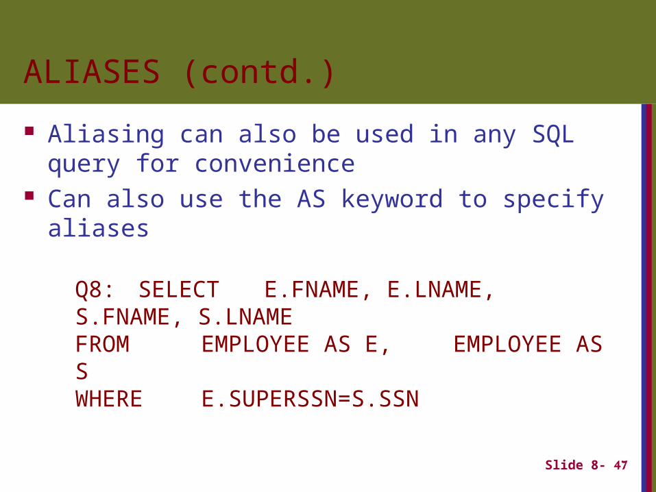
ALIASES (contd.)
Aliasing can also be used in any SQL query for convenience
Can also use the AS keyword to specify aliases
Q8: SELECT E.FNAME, E.LNAME, S.FNAME, S.LNAME
FROM EMPLOYEE AS E, EMPLOYEE AS S
WHERE E.SUPERSSN=S.SSN
Slide 8- 48
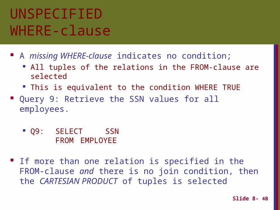
UNSPECIFIED WHERE-clause
A missing WHERE-clause indicates no condition; All tuples of the relations in the FROM-clause are selected This is equivalent to the condition WHERE TRUE
Query 9: Retrieve the SSN values for all employees.
Q9: SELECT SSNFROM EMPLOYEE
If more than one relation is specified in the FROM-clause and there is no join condition, then the CARTESIAN PRODUCT of tuples is selected
Slide 8- 49
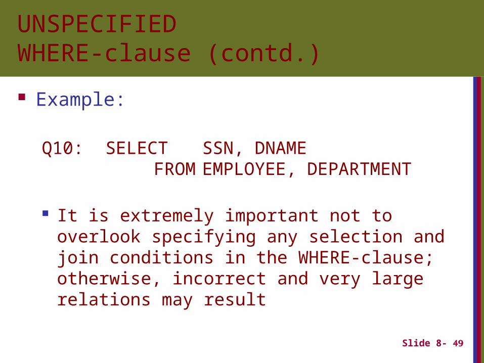
UNSPECIFIED WHERE-clause (contd.)
Example:
Q10: SELECT SSN, DNAMEFROM EMPLOYEE,
DEPARTMENT
It is extremely important not to overlook specifying any selection and join conditions in the WHERE-clause; otherwise, incorrect and very large relations may result
Slide 8- 50
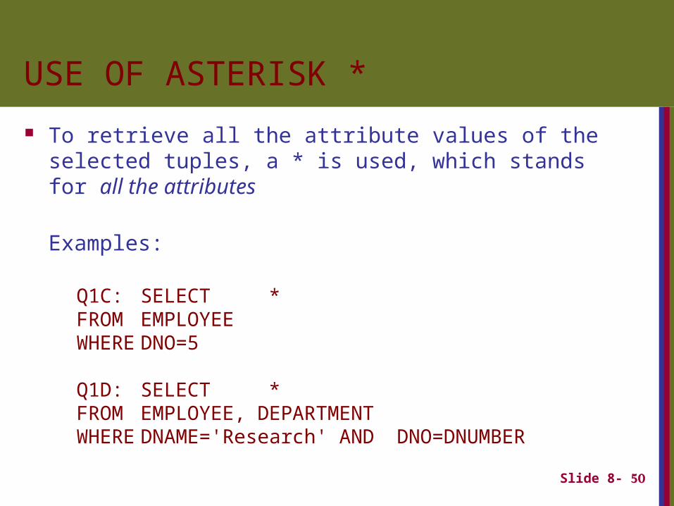
USE OF ASTERISK *
To retrieve all the attribute values of the selected tuples, a * is used, which stands for all the attributes
Examples:
Q1C: SELECT *FROM EMPLOYEEWHERE DNO=5
Q1D: SELECT *FROM EMPLOYEE, DEPARTMENTWHERE DNAME='Research' AND
DNO=DNUMBER
Slide 8- 51
USE OF DISTINCT
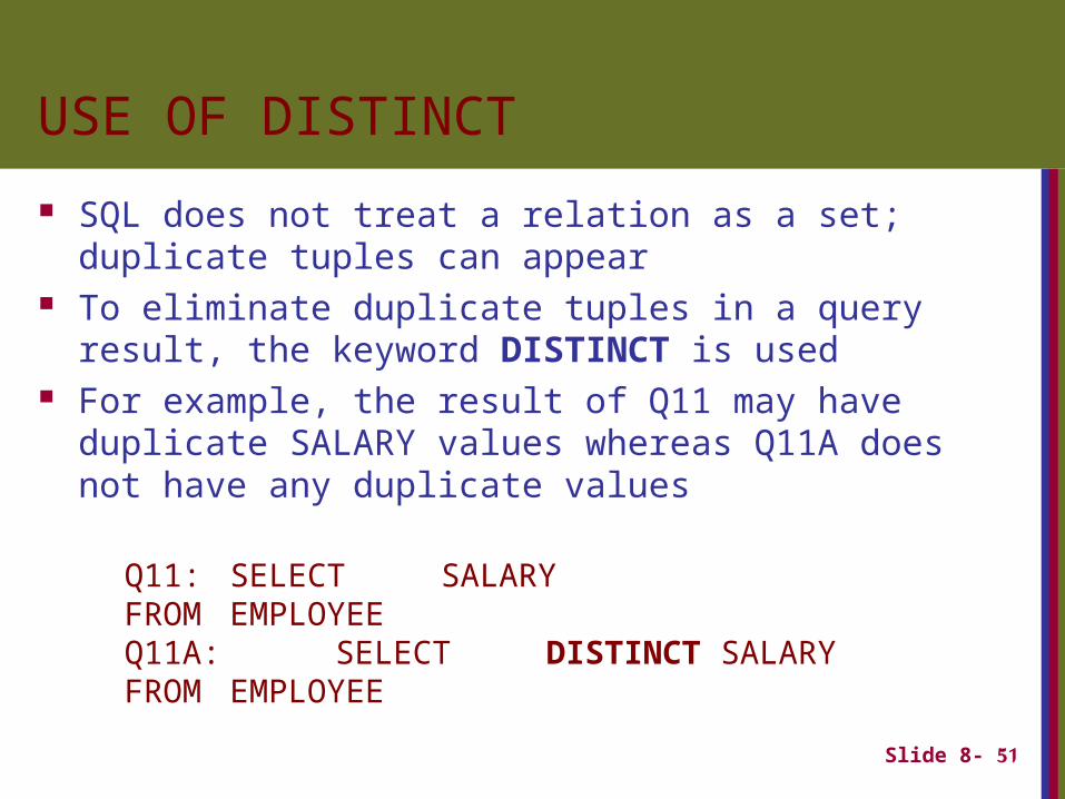
SQL does not treat a relation as a set; duplicate tuples can appear
To eliminate duplicate tuples in a query result, the keyword DISTINCT is used
For example, the result of Q11 may have duplicate SALARY values whereas Q11A does not have any duplicate values
Q11: SELECT SALARYFROM EMPLOYEE
Q11A: SELECT DISTINCT SALARYFROM EMPLOYEE
Slide 8- 52
SET OPERATIONS
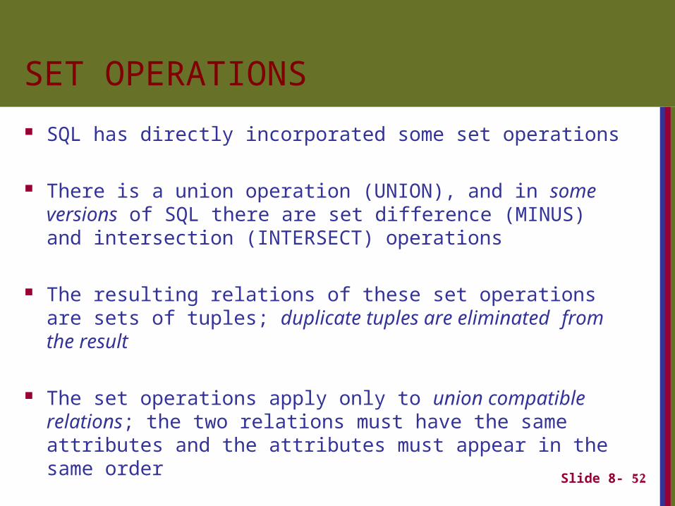
SQL has directly incorporated some set operations
There is a union operation (UNION), and in some versions of SQL there are set difference (MINUS) and intersection (INTERSECT) operations
The resulting relations of these set operations are sets of tuples; duplicate tuples are eliminated from the result
The set operations apply only to union compatible relations; the two relations must have the same attributes and the attributes must appear in the same order
Slide 8- 53
SET OPERATIONS (contd.)
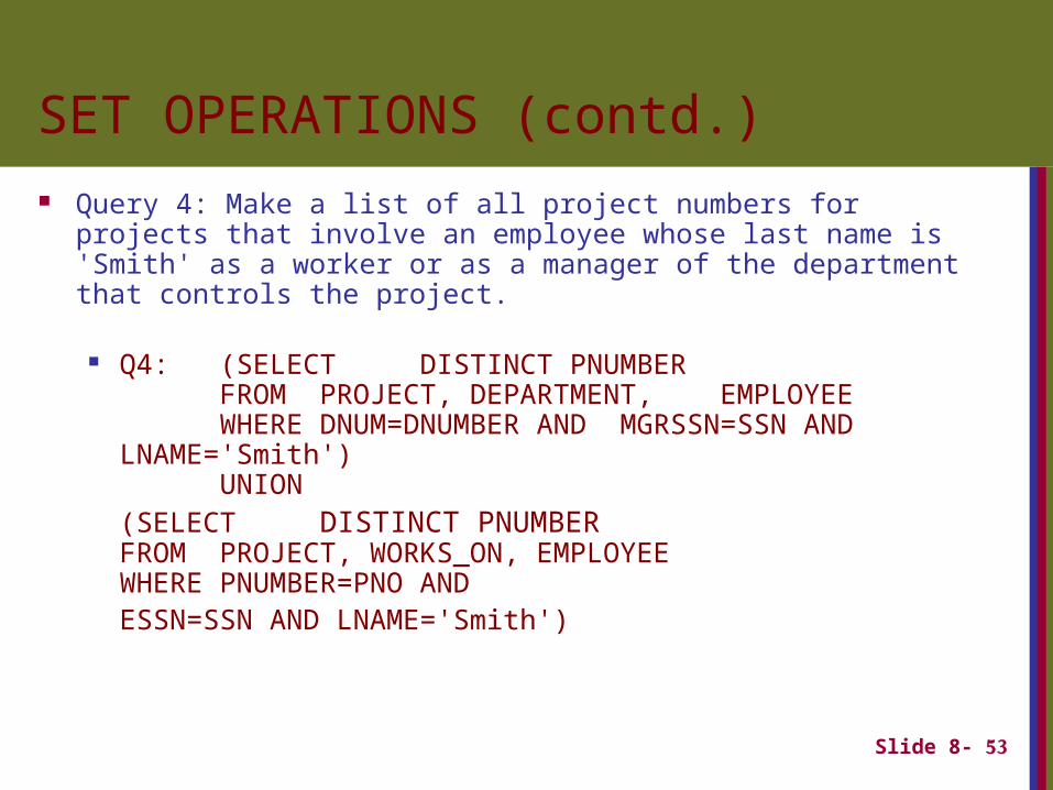
Query 4: Make a list of all project numbers for projects that involve an employee whose last name is 'Smith' as a worker or as a manager of the department that controls the project.
Q4: (SELECT DISTINCT PNUMBERFROM PROJECT, DEPARTMENT,
EMPLOYEEWHERE DNUM=DNUMBER AND
MGRSSN=SSN AND LNAME='Smith')
UNION(SELECT DISTINCT PNUMBER FROM PROJECT, WORKS_ON,
EMPLOYEEWHERE PNUMBER=PNO AND
ESSN=SSN AND LNAME='Smith')
Slide 8- 54
NESTING OF QUERIES
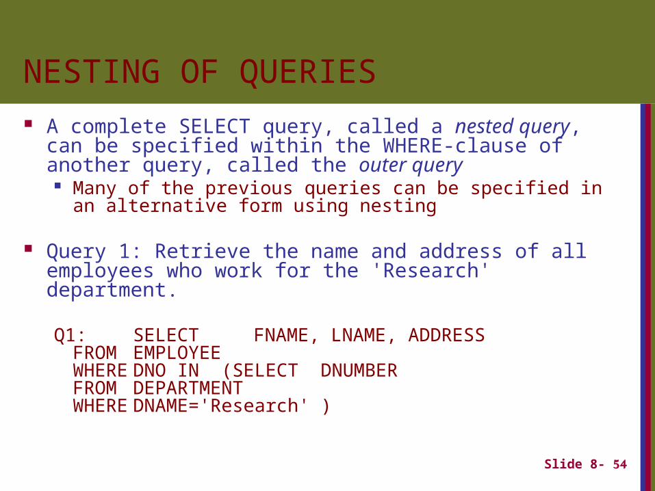
A complete SELECT query, called a nested query, can be specified within the WHERE-clause of another query, called the outer query
Many of the previous queries can be specified in an alternative form using nesting
Query 1: Retrieve the name and address of all employees who work for the 'Research' department.
Q1: SELECT FNAME, LNAME, ADDRESSFROM EMPLOYEEWHERE DNO IN (SELECT DNUMBERFROM DEPARTMENTWHERE DNAME='Research' )
Slide 8- 55
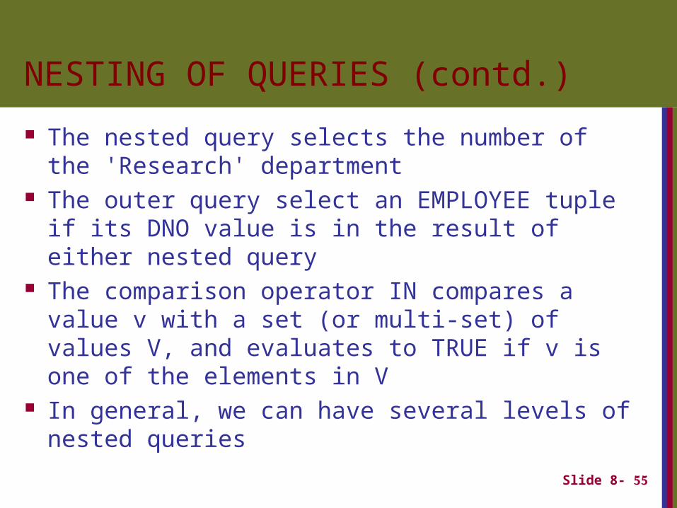
NESTING OF QUERIES (contd.)
The nested query selects the number of the 'Research' department
The outer query select an EMPLOYEE tuple if its DNO value is in the result of either nested query
The comparison operator IN compares a value v with a set (or multi-set) of values V, and evaluates to TRUE if v is one of the elements in V
In general, we can have several levels of nested queries
Slide 8- 56
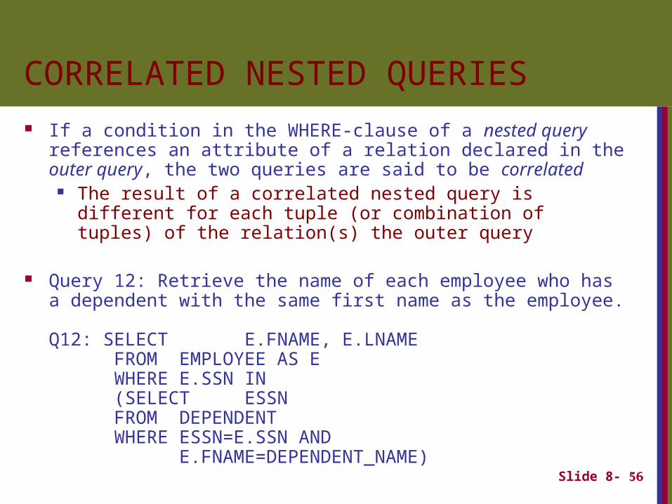
CORRELATED NESTED QUERIES
If a condition in the WHERE-clause of a nested query references an attribute of a relation declared in the outer query, the two queries are said to be correlated
The result of a correlated nested query is different for each tuple (or combination of tuples) of the relation(s) the outer query
Query 12: Retrieve the name of each employee who has a dependent with the same first name as the employee.
Q12: SELECT E.FNAME, E.LNAMEFROM EMPLOYEE AS EWHERE E.SSN IN
(SELECT ESSNFROM DEPENDENTWHERE ESSN=E.SSN AND
E.FNAME=DEPENDENT_NAME)

Slide 8- 57
CORRELATED NESTED QUERIES (contd.)
In Q12, the nested query has a different result in the outer query
A query written with nested SELECT... FROM... WHERE... blocks and using the = or IN comparison operators can always be expressed as a single block query. For example, Q12 may be written as in Q12A
Q12A: SELECT E.FNAME, E.LNAMEFROM EMPLOYEE E, DEPENDENT DWHERE E.SSN=D.ESSN AND
E.FNAME=D.DEPENDENT_NAME
Slide 8- 58
THE EXISTS FUNCTION
EXISTS is used to check whether the result of a correlated nested query is empty (contains no tuples) or not We can formulate Query 12 in an alternative form
that uses EXISTS as Q12B
Slide 8- 59
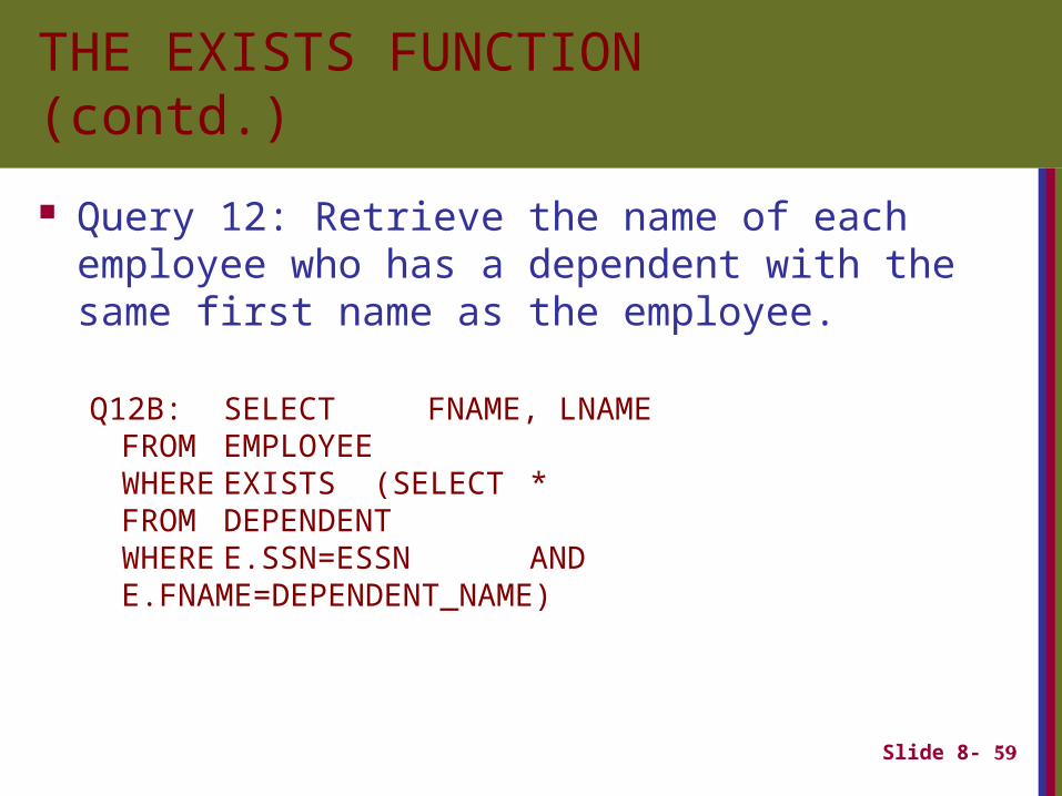
THE EXISTS FUNCTION (contd.)
Query 12: Retrieve the name of each employee who has a dependent with the same first name as the employee.
Q12B: SELECT FNAME, LNAMEFROM EMPLOYEEWHERE EXISTS (SELECT *
FROMDEPENDENT
WHEREE.SSN=ESSN AND
E.FNAME=DEPENDENT_NAME)
Slide 8- 60
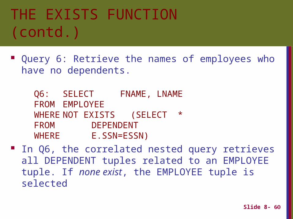
THE EXISTS FUNCTION (contd.)
Query 6: Retrieve the names of employees who have no dependents.
Q6: SELECT FNAME, LNAMEFROM EMPLOYEEWHERE NOT EXISTS (SELECT *
FROM DEPENDENT
WHERE E.SSN=ESSN)
In Q6, the correlated nested query retrieves all DEPENDENT tuples related to an EMPLOYEE tuple. If none exist, the EMPLOYEE tuple is selected
Slide 8- 61
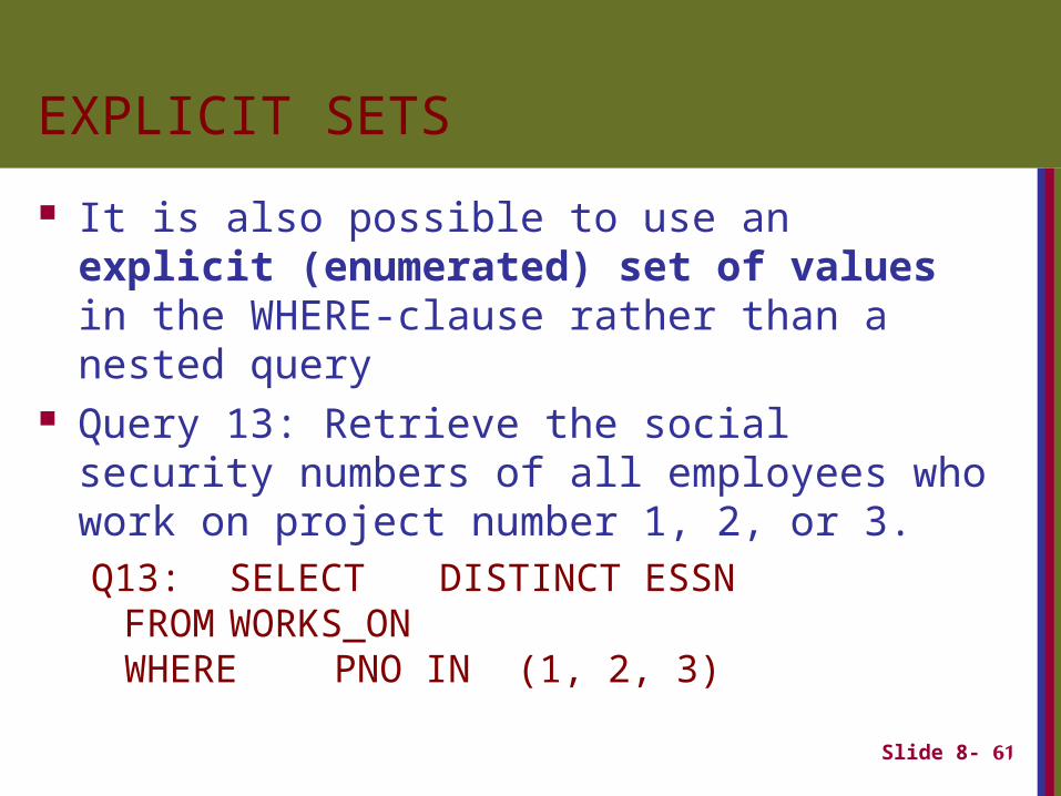
EXPLICIT SETS
It is also possible to use an explicit (enumerated) set of values in the WHERE-clause rather than a nested query
Query 13: Retrieve the social security numbers of all employees who work on project number 1, 2, or 3.Q13: SELECT DISTINCT ESSN
FROM WORKS_ONWHERE PNO IN (1, 2, 3)
Slide 8- 62
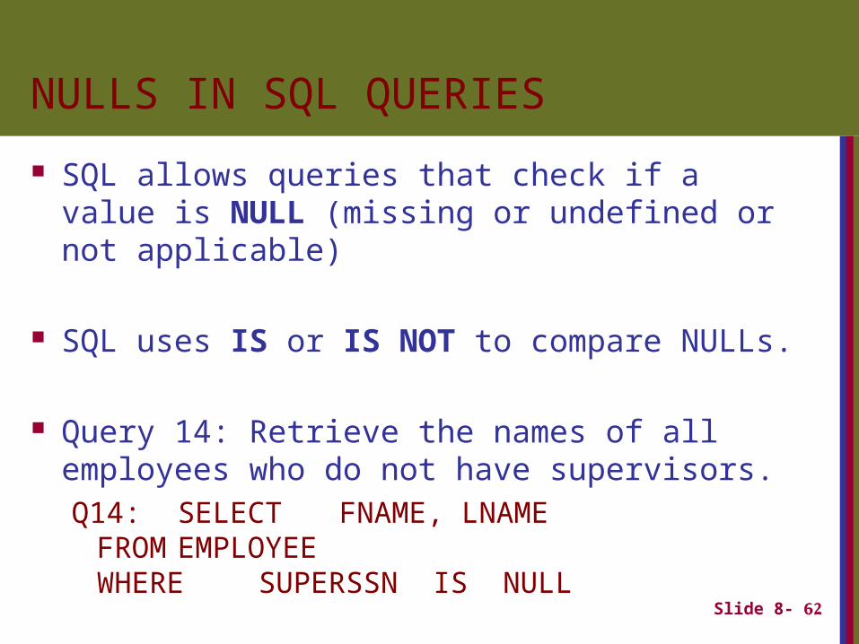
NULLS IN SQL QUERIES
SQL allows queries that check if a value is NULL (missing or undefined or not applicable)
SQL uses IS or IS NOT to compare NULLs.
Query 14: Retrieve the names of all employees who do not have supervisors.Q14: SELECT FNAME, LNAME
FROM EMPLOYEEWHERE SUPERSSN IS NULL
Slide 8- 63
Joined Relations Feature
Can specify a "joined relation" in the FROM-clause Looks like any other relation but is the result of a
join Allows the user to specify different types of joins
(regular "theta" JOIN, NATURAL JOIN, LEFT OUTER JOIN, RIGHT OUTER JOIN, CROSS JOIN, etc)
Slide 8- 64
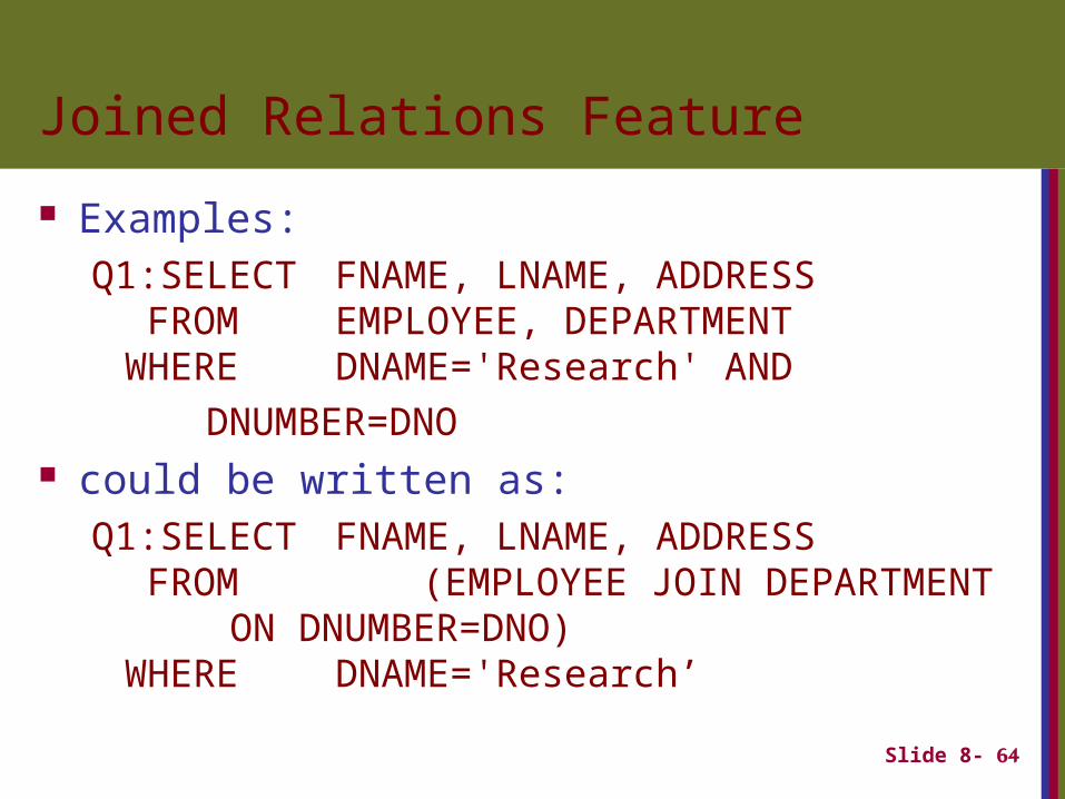
Joined Relations Feature
Examples:Q1:SELECT FNAME, LNAME, ADDRESS
FROM EMPLOYEE, DEPARTMENTWHERE DNAME='Research' AND
DNUMBER=DNO could be written as:
Q1:SELECT FNAME, LNAME, ADDRESS FROM (EMPLOYEE JOIN DEPARTMENT
ON DNUMBER=DNO)WHERE DNAME='Research’
Slide 8- 65
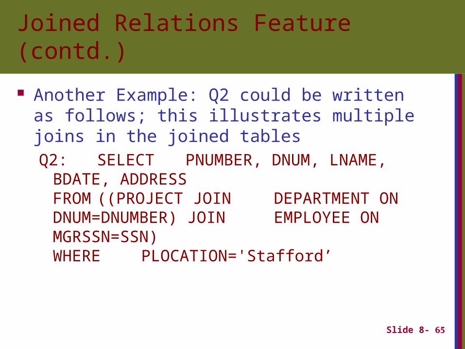
Joined Relations Feature (contd.)
Another Example: Q2 could be written as follows; this illustrates multiple joins in the joined tablesQ2: SELECT PNUMBER, DNUM, LNAME,
BDATE, ADDRESSFROM ((PROJECT JOIN
DEPARTMENT ON DNUM=DNUMBER)
JOIN EMPLOYEE ON MGRSSN=SSN)
WHERE PLOCATION='Stafford’
Slide 8- 66
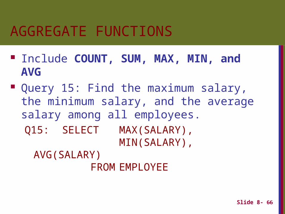
AGGREGATE FUNCTIONS
Include COUNT, SUM, MAX, MIN, and AVG Query 15: Find the maximum salary, the
minimum salary, and the average salary among all employees.Q15: SELECT MAX(SALARY),
MIN(SALARY), AVG(SALARY)FROM EMPLOYEE
Slide 8- 67
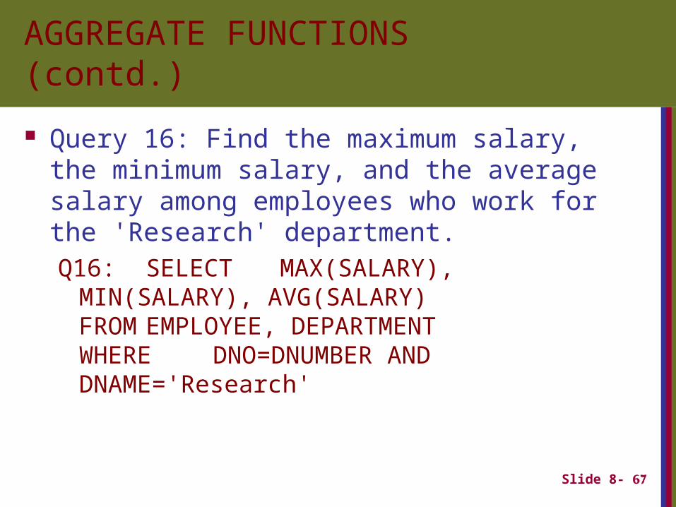
AGGREGATE FUNCTIONS (contd.)
Query 16: Find the maximum salary, the minimum salary, and the average salary among employees who work for the 'Research' department.Q16: SELECT MAX(SALARY),
MIN(SALARY), AVG(SALARY)FROM EMPLOYEE,
DEPARTMENTWHERE DNO=DNUMBER AND
DNAME='Research'
Slide 8- 68
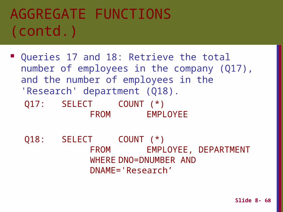
AGGREGATE FUNCTIONS (contd.)
Queries 17 and 18: Retrieve the total number of employees in the company (Q17), and the number of employees in the 'Research' department (Q18).Q17: SELECT COUNT (*)
FROM EMPLOYEE
Q18: SELECT COUNT (*)FROM EMPLOYEE, DEPARTMENTWHERE DNO=DNUMBER AND
DNAME='Research’
Slide 8- 69
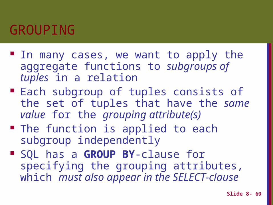
GROUPING
In many cases, we want to apply the aggregate functions to subgroups of tuples in a relation
Each subgroup of tuples consists of the set of tuples that have the same value for the grouping attribute(s)
The function is applied to each subgroup independently
SQL has a GROUP BY-clause for specifying the grouping attributes, which must also appear in the SELECT-clause
Slide 8- 70
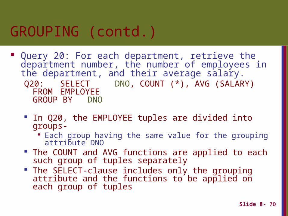
GROUPING (contd.)
Query 20: For each department, retrieve the department number, the number of employees in the department, and their average salary.Q20: SELECT DNO, COUNT (*), AVG (SALARY)
FROM EMPLOYEEGROUP BY DNO
In Q20, the EMPLOYEE tuples are divided into groups- Each group having the same value for the grouping attribute
DNO The COUNT and AVG functions are applied to each such
group of tuples separately The SELECT-clause includes only the grouping attribute
and the functions to be applied on each group of tuples
Slide 8- 71
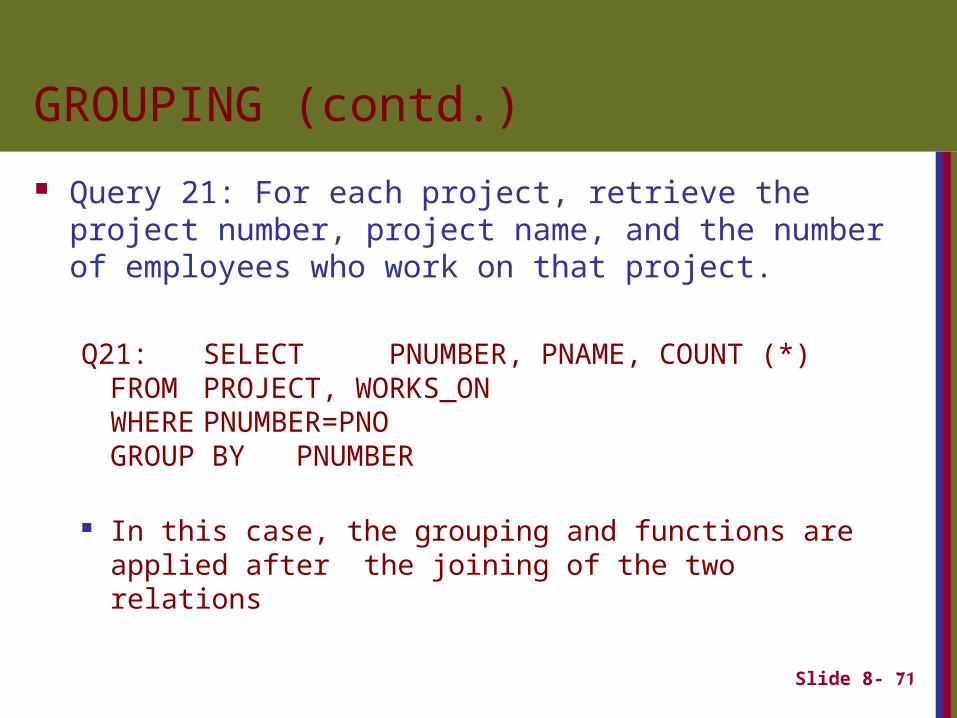
GROUPING (contd.)
Query 21: For each project, retrieve the project number, project name, and the number of employees who work on that project.
Q21: SELECT PNUMBER, PNAME, COUNT (*)FROM PROJECT, WORKS_ONWHERE PNUMBER=PNOGROUP BY PNUMBER
In this case, the grouping and functions are applied after the joining of the two relations


![Answering Conjunctive Queries under Updates - arxiv.org [8] and the studies of MSO queries on trees by Balmin, Papakonstantinou, and Vianu [5] and by Losemann and Martens [26], ...](https://static.fdocuments.us/doc/165x107/5af9c2787f8b9aac248ede05/answering-conjunctive-queries-under-updates-arxivorg-8-and-the-studies-of-mso.jpg)


