Slide 1 Statistics for HEP Roger Barlow Manchester University Lecture 3: Estimation.
23
Slide 1 Statistics for HEP Roger Barlow Manchester University Lecture 3: Estimation
-
date post
20-Dec-2015 -
Category
Documents
-
view
215 -
download
2
Transcript of Slide 1 Statistics for HEP Roger Barlow Manchester University Lecture 3: Estimation.

Slide 1
Statistics for HEPRoger Barlow
Manchester University
Lecture 3: Estimation

Slide 2
About Estimation
Theory Data
Statistical
Inference
TheoryData
Probability
Calculus
Given these distribution parameters, what can we
say about the data? Given this data, what can we say about the properties or parameters or correctness of
the distribution functions?

Slide 3
What is an estimator?
An estimator is a procedure giving a value for a parameter or property of the distribution as a function of the actual data values
2)ˆ(1
}{ˆ i
ixNxV
i
ixNx
1}{̂
2)ˆ(1
1}{ˆ
iixN
xV
2
}{ˆ minmax xxx

Slide 4
Minimum Variance Bound
What is a good estimator?
A perfect estimator is:• Consistent• Unbiassed
• Efficient minimum
aaLimitN
ˆ
adxdxaxPaxPaxPxxaa ...)...;();();(,...),(ˆ...ˆ 2132121
2ˆˆ)ˆ( aaaV
One often has to work with less-than-perfect estimators
2
2 ln
1)ˆ(da
LdaV
Slide 5
The Likelihood Function
Set of data {x1, x2, x3, …xN}
Each x may be multidimensional – never mind
Probability depends on some parameter a
a may be multidimensional – never mind
Total probability (density)
P(x1;a) P(x2;a) P(x3;a) …P(xN;a)=L(x1, x2, x3, …xN ;a)
The Likelihood

Slide 6
Maximum Likelihood Estimation
In practice usually maximise ln L as it’s easier to calculate and handle; just add the ln P(xi)
ML has lots of nice properties
0ˆ
aadA
dL
Given data {x1, x2, x3, …xN} estimate a by maximising the likelihood L(x1, x2, x3, …xN ;a)
a
Ln L
â
Slide 7
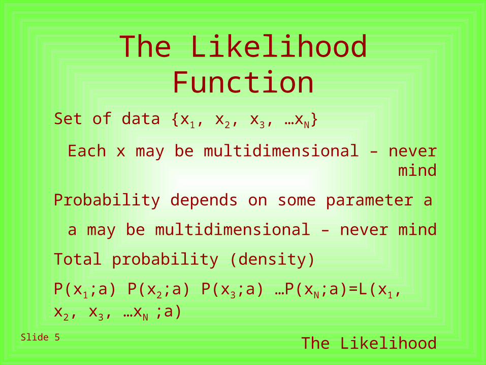
Properties of ML estimation• It’s consistent
(no big deal)• It’s biassed for small N
May need to worry• It is efficient for large N
Saturates the Minimum Variance Bound• It is invariant
If you switch to using u(a), then û=u(â)
a
Ln L
â u
Ln L
û

Slide 8
More about ML
• It is not ‘right’. Just sensible.
• It does not give the ‘most likely value of a’. It’s the value of a for which this data is most likely.
• Numerical Methods are often needed
• Maximisation / Minimisation in >1 variable is not easy
• Use MINUIT but remember the minus sign
Slide 9
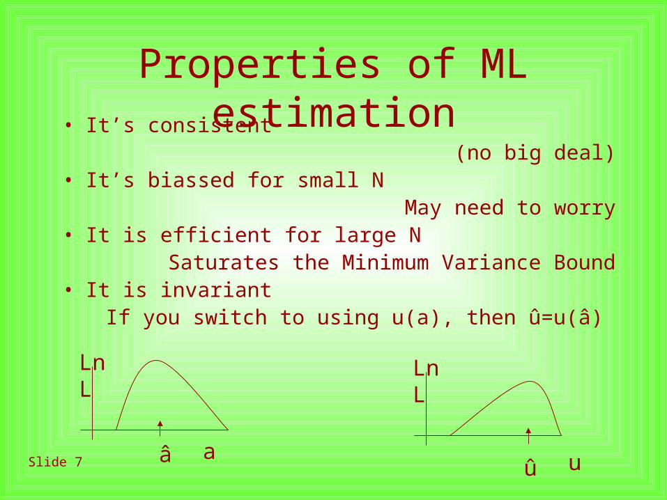
ML does not give goodness-of-fit
• ML will not complain if your assumed P(x;a) is rubbish
• The value of L tells you nothing
Fit P(x)=a1x+a0
will give a1=0; constant P
L= a0N
Just like you get from fitting

Slide 10
Least Squares
• Measurements of y at various x with errors and prediction f(x;a)
• Probability• Ln L
• To maximise ln L, minimise 2
22 2/));(( axfye 2
);(
2
1
ii
ii axfy
x
y
So ML ‘proves’ Least Squares. But what ‘proves’ ML? Nothing

Slide 11
Least Squares: The Really nice thing
• Should get 21 per data point• Minimise 2 makes it smaller – effect is 1
unit of 2 for each variable adjusted. (Dimensionality of MultiD Gaussian decreased by 1.)
Ndegrees Of Freedom=Ndata pts – N parameters
• Provides ‘Goodness of agreement’ figure which allows for credibility check
Slide 12
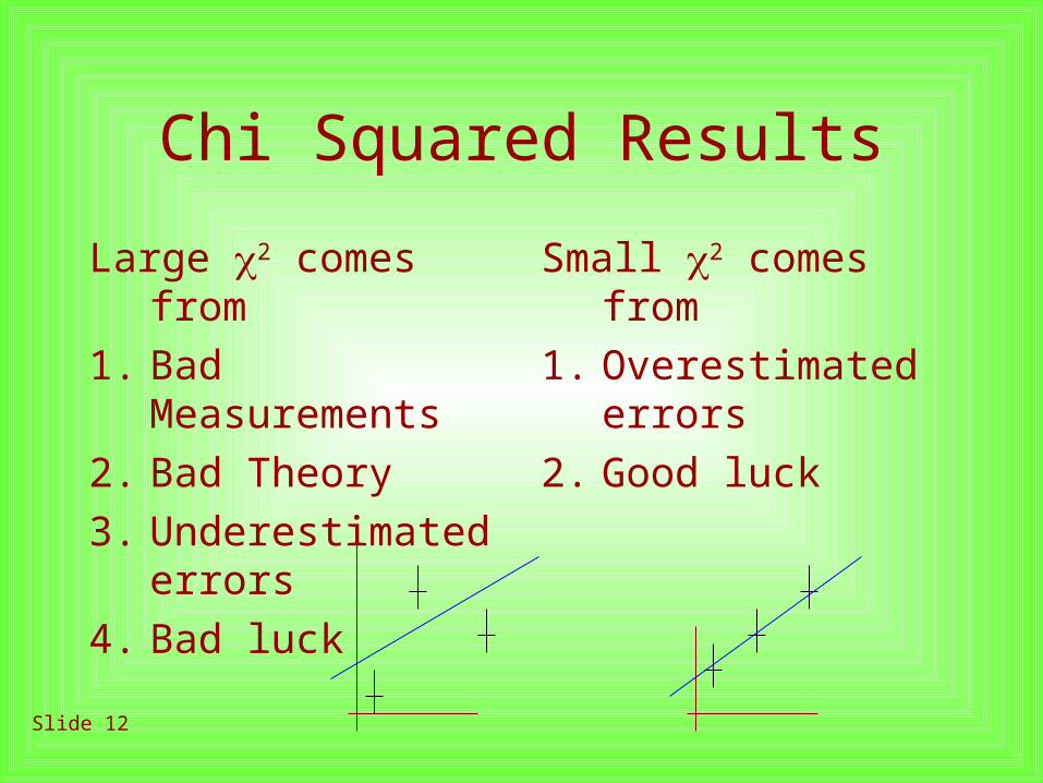
Chi Squared Results
Large 2 comes from
1. Bad Measurements
2. Bad Theory3. Underestimated
errors4. Bad luck
Small 2 comes from
1. Overestimated errors
2. Good luck
Slide 13
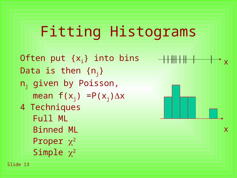
Fitting Histograms
Often put {xi} into bins
Data is then {nj}
nj given by Poisson,
mean f(xj) =P(xj)x4 Techniques
Full MLBinned MLProper 2
Simple 2
x
x
Slide 14
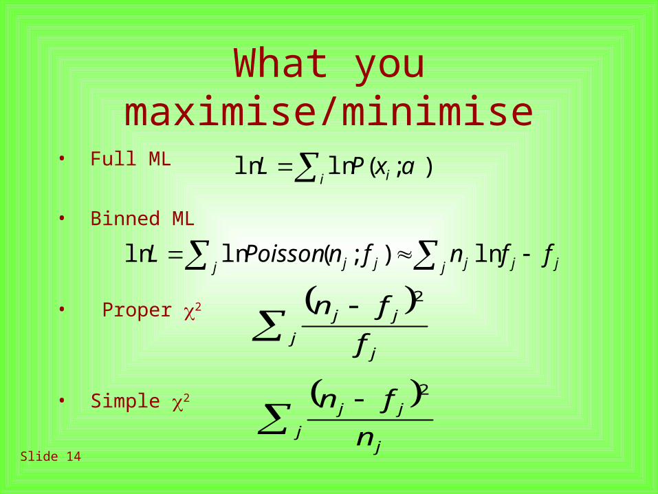
What you maximise/minimise
j j jjjjj ffnfnPoissonL ln);(lnln
j
j
jj
f
fn 2
j
j
jj
n
fn 2
• Full ML
• Binned ML
• Proper 2
• Simple 2
i i axPL );(lnln
Slide 15
Which to use?• Full ML: Uses all information but may be
cumbersome, and does not give any goodness-of-fit. Use if only a handful of events.
• Binned ML: less cumbersome. Lose information if bin size large. Can use 2 as goodness-of-fit afterwards
• Proper 2 : even less cumbersome and gives goodness-of-fit directly. Should have nj large so PoissonGaussian
• Simple 2 : minimising becomes linear. Must have nj large

Slide 16
Consumer tests show
• Binned ML and Unbinned ML give similar results unless binsize > feature size
• Both 2 methods get biassed and less efficient if bin contents are small due to asymmetry of Poisson
• Simple 2 suffers more as sensitive to fluctuations, and dies when bin contents are zero
Slide 17
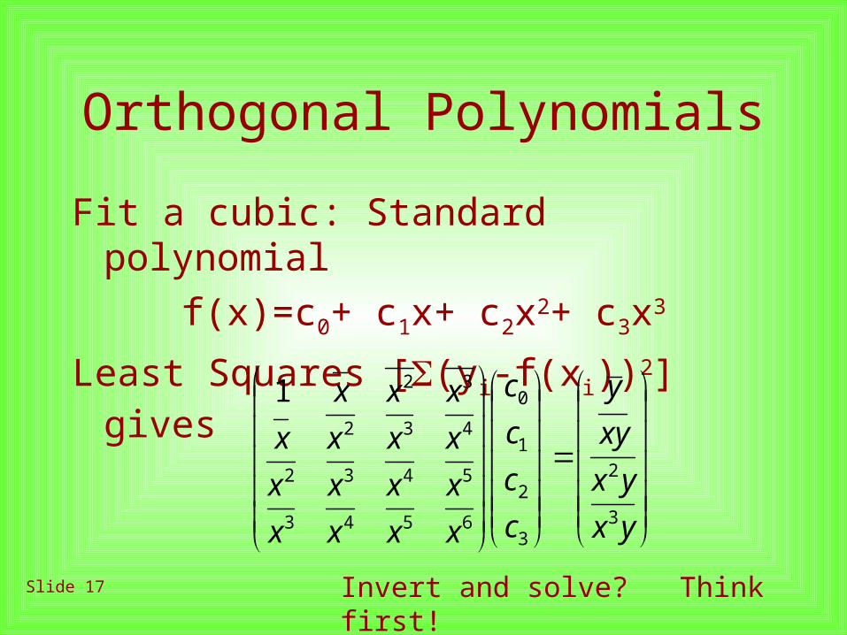
Orthogonal Polynomials
Fit a cubic: Standard polynomial f(x)=c0+ c1x+ c2x2+ c3x3
Least Squares [(yi-f(xi))2] gives
yx
yx
xy
y
c
c
c
c
xxxx
xxxx
xxxx
xxx
3
2
3
2
1
0
6543
5432
432
321
Invert and solve? Think first!
Slide 18
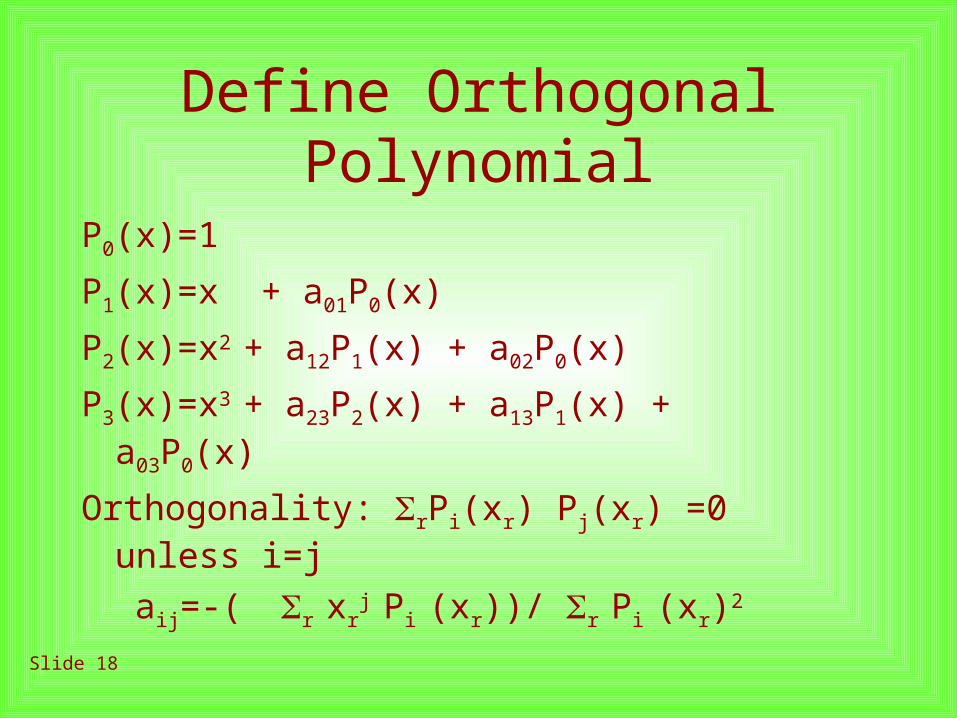
Define Orthogonal Polynomial
P0(x)=1
P1(x)=x + a01P0(x)
P2(x)=x2 + a12P1(x) + a02P0(x)
P3(x)=x3 + a23P2(x) + a13P1(x) + a03P0(x)
Orthogonality: rPi(xr) Pj(xr) =0 unless i=j
aij=-( r xrj Pi (xr))/ r Pi (xr)2

Slide 19
Use Orthogonal Polynomial
f(x)=c’0P0(x)+ c’1P1(x)+ c’2P2(x)+ c’3P3(x)
Least Squares minimisation givesc’i=yPi / Pi
2
Special Bonus: These coefficients are UNCORRELATED
Simple example: Fit y=mx+c ory=m(x -x)+c’
Slide 20
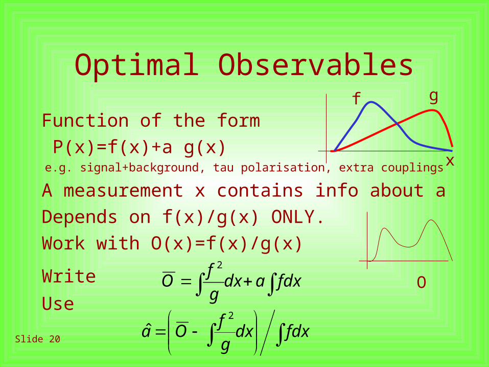
Optimal Observables
Function of the form P(x)=f(x)+a g(x)
e.g. signal+background, tau polarisation, extra couplings
A measurement x contains info about aDepends on f(x)/g(x) ONLY.Work with O(x)=f(x)/g(x)
Write Use
x
fdxadxg
fO
2
fdxdx
gf
Oa2
ˆ
g f
O
Slide 21
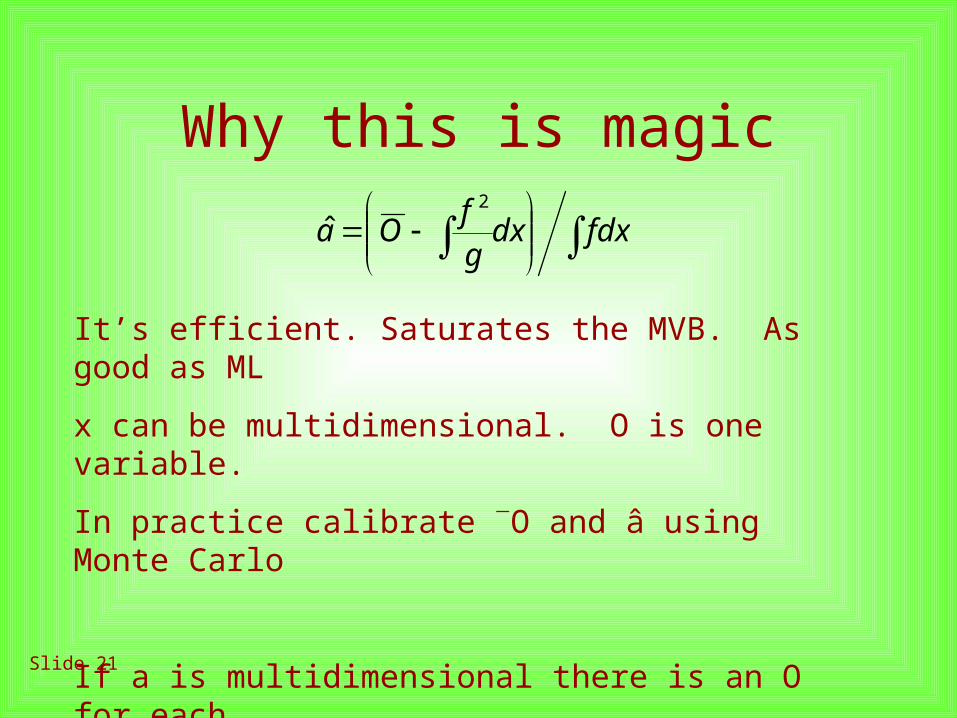
Why this is magic
fdxdx
gf
Oa2
ˆ
It’s efficient. Saturates the MVB. As good as ML
x can be multidimensional. O is one variable.
In practice calibrate O and â using Monte Carlo
If a is multidimensional there is an O for each
If the form is quadratic then use of the mean OO is not as good as ML. But close.
Slide 22
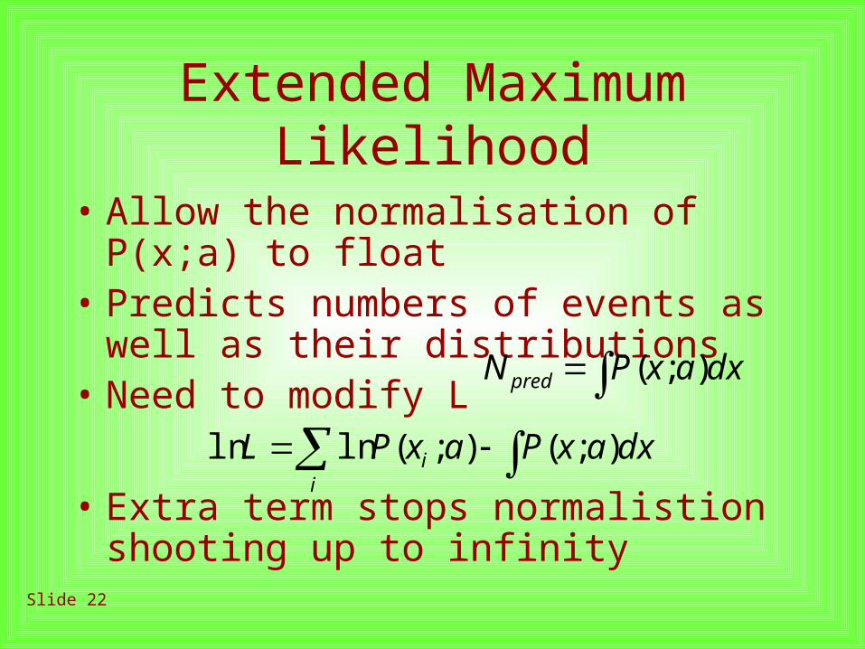
Extended Maximum Likelihood
• Allow the normalisation of P(x;a) to float
• Predicts numbers of events as well as their distributions
• Need to modify L
• Extra term stops normalistion shooting up to infinity
dxaxPaxPLi
i );();(lnln
dxaxPN pred );(

Slide 23
Using EML
• If the shape and size of P can vary independently, get same answer as ML and predicted N equal to actual N
• If not then the estimates are better using EML
• Be careful of the errors in computing ratios and such