Sketch Based 3D Modeling withCurvature Classification

Abstract

In this paper, we introduce a simple approach for sketching 3D models in arbitrary topology. Using this approach,we have developed a system to convert silhouette sketches to 3D meshes that mostly consists of quadrilaterals and4-valent vertices. Because of their regular structures, these 3D meshes can effectively be smoothed using Catmull-Clark subdivision. Our approach is based on the identification of corresponding points on a set of curves. Using thestructure of correspondences on the curves, we partition curves into junction, cap and tubular regions and constructmostly quadrilateral meshes using these partitions.

1. Introduction

Sketch based interfaces for modeling started almost20 years ago with the pioneering work by Tanaka et al.[1] and it gained significant attention with revolution-ary work by Igarashi et al. [2]. Since then a wide va-riety of methods have been introduced [3, 4]. In thispaper, we present a curvature based curve partitioningapproach for sketch based modeling of free-form 3Dshapes. For partitioning curves we have developed 2D-correspondence functions as an extension of shape di-ameter functions [5]. 2D-correspondence functions areused to identify correspondence points on curves andto robustly classify junction, cap and tubular regions ofcurves (see Figure 2). Based on this classification, itis easy to construct 3D meshes with mostly quadrilat-eral faces and 4-valent vertices. These meshes can ef-fectively be smoothed by Catmull-Clark subdivision [6]since they have only a few extraordinary vertices (seeFigure 1). We have also implemented the method todemonstrate the effectiveness of the new approach. Ourcurrent implementation construct 3D models only fromsketched silhouettes. We do not allow T-junctions (oc-cluded curves), which can provide additional informa-tion about the shapes [7, 8].

Our process for 3D sketching consists of 3 steps:curve construction, curve partitioning and mesh con-struction.(1) Curve Construction: This is a 1-manifold curve con-struction from a given set of arbitrary strokes. Section 3briefly describes this process.(2) Curve partitioning: This is the process of partition-ing the curves into positive, negative and zero curvature

regions using 2D-correspondence function. This is maincontribution of our paper and it is described in Section 4in detail.(3) Mesh construction. This is the final process that con-verts curves to 3D models. Section 5 provides a descrip-tion of this process.In the next section, we briefly discuss previous work onsketch based shape modeling.

2. Related Work

Sketch based modeling has been influential in creat-ing many exciting products and software. For instance,the ideas developed in papers [9] and [10] provided theconceptual basis of Sketchup software [11], which iswidely used for modeling simple architectural geometri-cal shapes. There also exists methods for modeling trees[12], modeling garments [13], modeling using symme-tries [14], modeling with 3D curve networks [15, 16],designing highways [17] and terrains [18].

In this paper, we are interested in sketching free formsmooth 3D shapes like Teddy [2], which is probably theone of the most influential work in sketch based mod-eling. Teddy is based on centroidal distance transformwhich is related to medial axis transform [19]. The dis-tance from a point on the boundary to the medial axisis the radius of the maximal ball, whose center lies onthe medial axis, touches the boundary at the point, andis completely contained in the object. This ball is calledthe medial-ball, and its radius can be seen as a form oflocal shape-radius connecting the boundary to the me-dial axis. The problem with medial axis transform isthat definition and extraction of the medial axis or even

Preprint submitted to Computer & Graphics February 22, 2012

(a) input stroke data (b) correspondence function applied (c) generated mesh (d) smoothed mesh

Figure 1: A Genus-2 Mesh created by our system. Our method can partition user drawn sketches shown in (a) into a set of junctions, tubes andcaps regions using a correspondence shown in (b). Using this partitioning it is easy to construct 3D models as shown in (c). These models caneffectively be smoothed since they consists mostly quadrilaterals as shown in (d).

of discrete approximations using skeletons are complexand often error prone [5]. Another problem with medialaxis transform is that the resulting meshes are usuallytriangulated, which may require a beautification step[20]. Our corresponding function approach, which is in-spired by 3D shape diameter function [5], is also relatedto medial axis transform but it is robust and guaranteesto construct meshes with mostly quadrilaterals and 4-valent vertices .

(a) input curves (b) curve region

(c) surface regions (d) 3D regions

Figure 2: Our correspondence function allows us to robustly classifythe portions of curves as junctions, caps and tubes. These regions cor-respond zero, negative and positive total Gaussian curvature regions.After this classification, it is easy construct 3D mesh surfaces thatconsist of mostly quadrilateral faces.

Our work is also related to Sketch-based subdivisionmethod [21], which presents a sketch-based interface todesign subdivision models. By taking profile curves ofthe surface as an input, it generates a coarse and quaddominant control mesh with few extraordinary verticesor faces. The corresponding limit surface interpolates

the profile curves with the capability of local controlacross these curves and of the model in general. How-ever, this approach creates models that are extrusions ofthe profile curves in z direction by resulting a flat look-ing model. Our approach can be seen as a combinationof the organic look of [2] and smoothness achieved bysubdivision surfaces suggested by Nasri et al. [21].

Implicit surfaces provide an alternative for sketch-ing free form smooth surfaces which includes convo-lution surfaces [22], Variational Hermite-RBF implicits[23], Shapeshop [24] and others [25, 26, 27, 28, 29].Since implicit surfaces can provide exact and approx-imate set operations, they are particularly attractive tomodel complicated surfaces. In this work, we do notuse an implicit based approach.

3. Curve Construction

We assume that the initial silhouette is drawn as aset of unorganized strokes. The directions of strokesmay not be consistent with how artists would draw.We assume that there is no self-intersections and/or T-junctions. Each stroke is represented as a poly-line.Curve construction process combine, resample and re-order these strokes in such a way that at the end ofthe process we obtain 1-manifold with well-defined in-side and outside. In practice, we allow 1-manifold withboundaries and we can still obtain consistent normals.

Curve construction starts with combining individualstrokes into longer curves. This process converts thestrokes to a set of closed or open parameterized poly-lines. We then re-sample the curves in equal distancessuch that the resulting curves are independent of thespeed of the sketching. We then turn the curves into 1-manifolds by giving a rotation order to each curve suchthat always right side indicates inside of the curve. Thisis done by using classical inside-outside test. This pro-cess connects the points by single-links that provide a

2

consistent rotation direction. We call the resulting set ofcurves 1-manifold since they can define a closed shapein 2D. For each sample point i, we record and calculatethe position Ci, normal Ni and tangent Ti.

4. Curve Partitioning with Point Classification

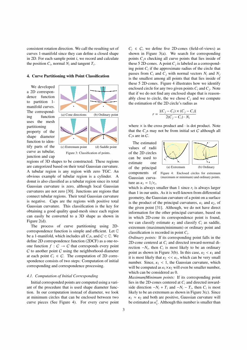
(a) Cone directions (b) Ordinary point

(c) Extremum point (d) Saddle point

Figure 3: Classification of points.

We developeda 2D correspon-dence functionto partition 1-manifold curves.The correspond-ing functionuses the meshpartitioningproperty of theshape diameterfunction to iden-tify parts of thecurve as tubular,junction and capregions of 3D shapes to be constructed. These regionsare categorized based on their total Gaussian curvature.A tubular region is any region with zero TGC. Anobvious example of tubular region is a cylinder. Adonut is also classified as a tubular region since its totalGaussian curvature is zero, although local Gaussiancurvatures are not zero [30]. Junctions are regions thatconnect tubular regions. Their total Gaussian curvatureis negative. Caps are the regions with positive totalGaussian curvature. This classification is the key forobtaining a good quality quad-mesh since each regioncan easily be converted to a 3D shape as shown inFigure 2(d).

The process of curve partitioning using 2D-correspondence function is simple and efficient. Let Cbe a 1-manifold, which includes all Cis, and C ⊂ C. Wedefine 2D correspondence function (2DCF) as a one-to-one function f : C → C that corresponds every pointC to another point C using the neighborhood-diameterat each point Ci ∈ C. The computation of 2D corre-spondence consists of two steps: Computation of initialcorresponding and correspondence processing.

4.1. Computation of Initial Corresponding

Initial corresponded points are computed using a vari-ant of the procedure that is used shape diameter func-tion. In our computation instead of diameter, we lookat minimum circles that can be enclosed between twocurve pieces (See Figure 4). For every curve point

Ci ∈ C, we define five 2D-cones (field-of-views) asshown in Figure 3(a). We search for correspondingpoints C js checking all curve points that lies inside ofthese 5 2D-cones. A point C j is labeled as a correspond-ing point Ci if the approximate radius of the circle thatpasses from Ci and C j with normal vectors Ni and N j

is the smallest among all points that that lies inside ofthese 5 2D-cones. Figure 4 illustrates how we identifyenclosed circle for any two given points Ci and C j. Notethat if we do not find any enclosed shape that is reason-ably close to circle, the we chose C j and we computethe estimation of the 2D circle’s radius as

r =|(C j −Ci) × (C j −Ci)|

2(C j −Ci) · Ni

where × is the cross product and · is dot product. Notethat the C js may not be from initial set C although allCis are in C.

(a) Extremum (b) Ordinary

Figure 4: Enclosed circles for extremum(maximum or minimum) and ordinary points.

The estimatedvalues of radiiof the 2D circlescan be used toestimate oneof the principalcomponents ofGaussian curva-ture as κ1 = 1/ri,which is always smaller than 1 since ri is always largerthan 1 in our units. As it is well-known from differentialgeometry, the Gaussian curvature of a point on a surfaceis the product of the principal curvatures, κ1 and κ2, ofthe given point [31]. Although, we do not have directinformation for the other principal curvature, based onin which 2D-cone its correspondence point is found,we can classify estimate κ2 and classify Ci as saddle,extremum (maximum/minimum) or ordinary point andclassification is recorded in point Ci.Ordinary points: If its corresponding point falls in the2D-cone centered at Ci and directed inward-normal di-rection −Ni, then Ci is most likely to be an ordinarypoint as shown in Figure 3(b). In this case, κ2 < κ1 andit is most likely that κ2 << κ1, which can be very smallnumber. Since, κ1 < 1, the Gaussian curvature, whichwill be computed as κ1×κ2 will even be smaller number,which can be considered as 0.Maximum/Minimum points: If its corresponding pointlies in the 2D-cones centered at Ci and directed inward-side direction −Ni + Ti and −Ni − Ti, then Ci is mostlikely to be an extremum as shown in Figure 3(c). Sinceκ1 ≈ κ2 and both are positive, Gaussian curvature willbe estimated as κ2

1. Although this number is smaller than

3

κ1, it is still a relatively large number comparing Gaus-sian curvatures of ordinary points.Saddle points: If its corresponding point lies in 2D-cones centered at Ci and directed outward-side direc-tion Ni + Ti and Ni − Ti, then Ci is most likely to be asaddle as shown in Figures 3(c) and 5(b). In this case.κ1 will be a negative number since the enclosed circleis found outside. There is another way to identify sad-dle points. If more than one ordinary point correspondto the same point C j as shown in Figure 5(a), they arealso considered saddle points. Using this additional in-formation, we actually estimate κ2, which is a positivenumber computed as curvature of ordinary points thatchooses C j as their correspondence.

The Gaussian curvature obtained from correspon-dence data is very noisy and includes some correspon-dence information (e.g. correspondence from saddlepoints) that is not needed to construct 3D model. Shapediameter function computation uses median filtering toremove similar type of noise. We, instead, process thecorrespondence data to distribute Gaussian curvatureamong the neighbors to remove the noise.

4.2. Correspondence Processing

Correspondence processing distributes the Gaussiancurvature among the neighbors. This process consistsof sx steps:1. Updating C: We extend C, to include all C js inaddition to original Cis.

(a) To saddle point (b) From saddle point

Figure 5: Correspondence to and from saddlepoints.

2. Splittingone-to-manycorrespon-dences: Asillustrated inFigure 5(a),more thanone ordinarypoint can

correspond to a saddle point, resulting in one-to-manycorrespondences. When this happens, we simply moveone correspondence to one of the neighborhood pointsuntil we obtain a one-to-one correspondence.3. Removing useless correspondences: We removecorrespondences of saddle points from C. As illustratedin Figure 5(b), since these correspondences go outsideof the shape, they are actually useless except for classi-fying the point as saddle and computing an estimate ofGaussian curvature.4. Reassign correspondences: Since correspondencesare now one-to-one, both ends of the corresponding

function refer to each other.5. Laplacian smoothing: We take the immediateneighbors of the point that we proccess. The parametricaverage of the correspondences of these neigbors

To do Laplacian smoothing we take the correspond-ing points of our intiail point’s neighbors. We thenmove the correspondence of our initial point to theparametric average of these corresponding points. Thisoperation removes the Gaussian noise resulted frominitial computation. Note that this operation replacessome of the elements of C with new points from thewhole set C.

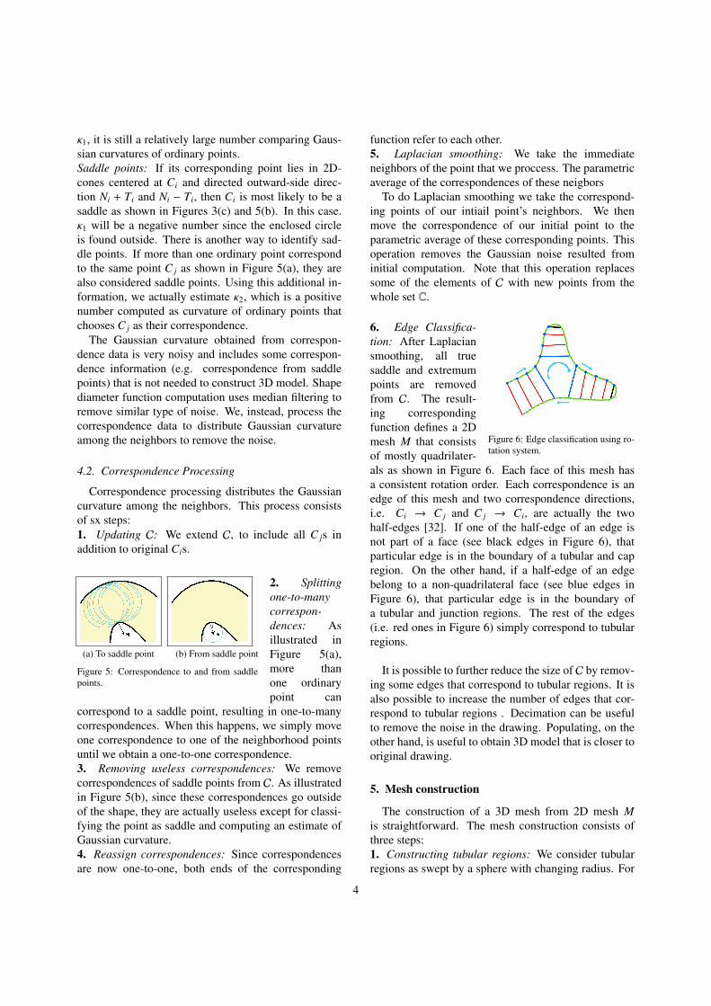
Figure 6: Edge classification using ro-tation system.

6. Edge Classifica-tion: After Laplaciansmoothing, all truesaddle and extremumpoints are removedfrom C. The result-ing correspondingfunction defines a 2Dmesh M that consistsof mostly quadrilater-als as shown in Figure 6. Each face of this mesh hasa consistent rotation order. Each correspondence is anedge of this mesh and two correspondence directions,i.e. Ci → C j and C j → Ci, are actually the twohalf-edges [32]. If one of the half-edge of an edge isnot part of a face (see black edges in Figure 6), thatparticular edge is in the boundary of a tubular and capregion. On the other hand, if a half-edge of an edgebelong to a non-quadrilateral face (see blue edges inFigure 6), that particular edge is in the boundary ofa tubular and junction regions. The rest of the edges(i.e. red ones in Figure 6) simply correspond to tubularregions.

It is possible to further reduce the size of C by remov-ing some edges that correspond to tubular regions. It isalso possible to increase the number of edges that cor-respond to tubular regions . Decimation can be usefulto remove the noise in the drawing. Populating, on theother hand, is useful to obtain 3D model that is closer tooriginal drawing.

5. Mesh construction

The construction of a 3D mesh from 2D mesh Mis straightforward. The mesh construction consists ofthree steps:1. Constructing tubular regions: We consider tubularregions as swept by a sphere with changing radius. For

4

every edge of M, i.e. Ci−C j pair, we place a sphere witha radius of the 2D circle that correspond the edge of M.We adjust the center of the sphere in such a way that therays coming from eye are tangent to the sphere. This ad-justment guarantees the correct silhouette. The centersof these spheres form skeletal 3D curves that are medialto the tubular regions. After choosing a great circle foreach sphere perpendicular to the skeletal 3D curve, wecan construct edge loops by connecting equidistant ver-tices placed around these circles. We then connect theseedge loops to construct tubular meshes in 3D. This pro-cess creates not one but a set of disconnected tubularmeshes.2.

Combining tubular regions with junctions: We con-nect the tubular meshes using junction regions in the2D mesh. For the border edges around each junction re-gion, we retrieve the edge loops constructed for them.We then connect the vertices of each half of an edgeloop to the adjacent half in the consequtive edge looporder one by one in the rotation .3. Adding caps: We can optionally cover the open polesof the tubular mesh with caps.

We have developed a simple sketch based model-ing system to show the feasibility of our method. Theshapes shown in Figures 1, 8 and 7 are examples thatare created using our system.

Figure 7: A genus-3 manifold mesh created by our system.

6. Conclusion and Discussion

This paper introduced an approach for sketching 3Dmodels of arbitrary genus. Our approach provides theorganic (non-flat) look obtained by Igarashi [2]. We de-veloped a system to convert silhouette sketches to 3Dmeshes that mostly consists of regular quadrilaterals.Because of their regular structures, these 3D meshes can

effectively be smoothed using Catmull-Clark subdivi-sion similar to Sketch-based subdivision method intro-duced by Nasri et al. [21]. We have introduced a robustcorrespondence function, which can be used as an alter-native to medial axis transformation and shape diame-ter functions in applications other than sketch modelingsince it can also help to partition even surfaces into ex-tremum, saddle or ordinary regions.

Our correspondence processing is a non-linear opera-tion that implicitly provides total Gaussian curvature ina given region. Therefore, we do not fully utilize theexpected Gaussian curvature information we have ob-tained. However, this information can be useful to cre-ate even better meshes by directly controlling vertex andface defects by creating 3 or 5-valence vertices [30].

Figure 8: A genus-0 manifold mesh created by our system.

We have also implemented a simple user interface todemonstrate the effectiveness of the new approach. Ourcurrent implementation can construct 3D models onlyfrom sketched silhouettes. We do not allow T-junctionsincluding occluded curves. Such T-junctions are es-sential to create more complicated shapes [7, 8]. Ourmethod can only create shapes whose medial axis are1-complexes, i.e. a connected set of 3D curves. Me-dial axes of general shapes can be 2-complexes. Ourmethod is specifically useful for the development of in-terfaces for cartoonists who draw and develop charac-ters that consists of tubular regions connected by junc-tions [33, 34].

References

[1] T. Tanaka, S. Naito, T. Takahashi, Generalized symmetry and itsapplication to 3d shape generation, The Visual Computer 5 (1-2)(1989) 8394.

5

[2] T. Igarashi, S. Matsuoka, H. Tanaka, A sketching interface for3d freeform design, in: Proceedings of ACM SIGGRAPH’99,1999, pp. 409–416.

[3] L. Olsen, F. F. Samavati, M. C. Sousa, J. A. Jorge, Sketch-basedmodeling: A survey, Computers & Graphics 33 (2) (2009) 85–103.

[4] J. LaViola, Sketch-based interfaces: techniques and applica-tions, ACM SIGGRAPH 2007 courses, 2007.

[5] L. Shapira, A. Shamir, D. Cohen-Or, Consistent mesh partition-ing and skeletonisation using the shape diameter function, Vi-sual Computing 24 (4) (2008) 249259.

[6] E. Catmull, J. Clark, Recursively generated b-spline surfaceson arbitrary topological meshes, Computer Aided Design (10)(1978) 350–355.

[7] O. Karpenko, J. Hughes, R. raskar, Smoothsketch: 3d free-form shapes from complex sketches, Proceedings of ACM SIG-GRAPH2006 30 (3) (2006) 589597.

[8] F. Cordier, H. Seo, Free-form sketching of self-occluding ob-jects, IEEE Computer Graphics and Applications 27 (1) (2007)5059.

[9] J. F. H. R. C. Zeleznik, K. P. Herndon, Sketch: An interface forsketching 3d scenes, in: Proceedings SIGGRAPH 96, 1996, pp.163–170.

[10] T. Igarashi, J. Hughes, A suggestive interface for 3d drawing, in:Proceedings of UIST’01, 2001, pp. 173–181.

[11] Google, Sketchup software, www.sketchup.com (2010).[12] M. Okabe, S. Owada, T. Igarashi, Interactive design of botanical

trees using free hand sketches and example-based editing, Com-puter Graphics Forum (Eurographics05) 24 (3) (2005) 487496.

[13] E. Turquin, M.-P. Cani, J. F. Hughes, Sketching garments forvirtual characters.

[14] A. C. Oztireli, U. Uyumaz, T. Popa, A. Sheffer, M. Gross,3d modeling with a symmetric sketch, in: Proceedings of theEighth Eurographics Symposium on Sketch-Based Interfacesand Modeling, SBIM ’11, 2011, pp. 23–30.

[15] S. Morigi, M. Rucci, Reconstructing surfaces from sketched 3dirregular curve networks, in: Proceedings of the Eighth Euro-graphics Symposium on Sketch-Based Interfaces and Modeling,SBIM ’11, 2011, pp. 39–46.

[16] G. Orbay, L. B. Kara, Sketch-based modeling of smooth sur-faces using adaptive curve networks, in: Proceedings of theEighth Eurographics Symposium on Sketch-Based Interfacesand Modeling, SBIM ’11, 2011, pp. 71–78.

[17] C. S. Applegate, S. D. Laycock, A. M. Day, A sketch-basedsystem for highway design, in: Proceedings of the Eighth Euro-graphics Symposium on Sketch-Based Interfaces and Modeling,SBIM ’11, 2011, pp. 55–62.

[18] M.-P. Cani, Sketching terrain, Tech-nical Report, LJK/EVASION, www-evasion.imag.fr/Positions/sujets/masterSketchTerrain2008.pdf(2008).

[19] H. Choi, S. Choi, H. Moon, Mathematical theory of medial axistransform, Pacific Journal of Mathematics 181 (1) (1997) 5788.

[20] T. Igarashi, J. Hughes, Smooth meshes for sketch-basedfreeform modeling, in: Proceedings of Symposium on Interac-tive 3D Graphics, 2003, p. 139142.

[21] A. Nasri, W. B. Karam, F. Samavati, Sketch-based subdivisionmodels, in: Proceedings of the 6th Eurographics Symposiumon Sketch-Based Interfaces and Modeling, SBIM ’09, 2009, pp.53–60.

[22] A. Alexe, L. Barthe, M.-P. Cani, Shape modeling by sketchingusing convolution surfaces, in: Proceedings of Pacific Graphics,2005.

[23] E. V. Brazil, I. Macedo, M. C. Sousa, L. H. de Figueiredo,L. Velho, Sketching variational hermite-rbf implicits, in: Pro-

ceedings of the Seventh Sketch-Based Interfaces and ModelingSymposium, SBIM ’10, 2010, pp. 1–8.

[24] R. Schmidt, B. Wyvill, C. M. Sousa, J. Jorge, Shapeshop:Sketch-based solid modeling with blobtrees (2005) 53–62.

[25] M. P. C. L. B. A. Bernhardt, A. Pihuit, Matisse: Painting 2dregions for modeling free-form shapes, in: EUROGRAPHICSWorkshop on Sketch-Based Interfaces and Modeling,(2008) C.Alvarado and M.- P. Cani (Editors), 2008.

[26] O. Karpenko, J. Hughes, R. Raskar, Free-form sketching withvariational implicit surfaces, Proceedings of Eurographics200221 (3) (2002) 585594.

[27] R. Schmidt, Interactive modeling with implicit surfaces, The-sis, Department of Computer Science, University of Calgary,Canada (2006).

[28] R. Schmidt, P. J. T. Isenberg, K. Singh, B. Wyvill, Sketching,scaffolding, and inking: A visual history for interactive 3d mod-eling, Proceedings of NPAR 2007.

[29] R. Schmidt, K. Singh, R. Balakrishnan, Sketching and com-posing widgets for 3d manipulation, Proceedings of EURO-GRAPHICS 2008, Editors: G. Drettakis and R. Scopigno 27 (2).

[30] E. Akleman, J. Chen, Practical polygonal mesh modeling withdiscrete gauss-bonnet theorem, in: Proceedings of GeometryModeling and Processing (GMP’06), 2006, pp. 287–298.

[31] E. W. Weisstein, Gaussian Curvature, FromMathWorld–A Wolfram Web Resource,http://mathworld.wolfram.com/GaussianCurvature.html,2011.

[32] M. Mantyla, An Introduction to Solid Modeling, Computer Sci-ence Press, Rockville, Ma., 1988.

[33] S. Lee, J. Buscema, How to Draw Comics the Marvel Way, Si-mon & Schuster, Inc., New York, 1984.

[34] S. McCloud, Understanding Comics: The Invisible Art, CollinsPublishers, Inc., New York, 1994.

6