Nature | www.nature.com | 1

Article

Six reference-quality genomes reveal evolution of bat adaptations

David Jebb, Zixia Huang, Martin Pippel, Graham M. Hughes, Ksenia Lavrichenko, Paolo Devanna, Sylke Winkler, Lars S. Jermiin, Emilia C. Skirmuntt, Aris Katzourakis, Lucy Burkitt-Gray, David A. Ray, Kevin A. M. Sullivan, Juliana G. Roscito, Bogdan M. Kirilenko, Liliana M. Dávalos, Angelique P. Corthals, Megan L. Power, Gareth Jones, Roger D. Ransome, Dina K. N. Dechmann, Andrea G. Locatelli, Sébastien J. Puechmaille, Olivier Fedrigo, Erich D. Jarvis20,, Michael Hiller ✉, Sonja C. Vernes ✉, Eugene W. Myers ✉ & Emma C. Teeling ✉

In the format provided by the authors and unedited

Supplementary information

https://doi.org/10.1038/s41586-020-2486-3

Nature | www.nature.com/nature

1

Supplementary Information

Title: Six reference-quality genomes reveal evolution of bat adaptations

David Jebb^1,2,3

, Zixia Huang^4, Martin Pippel^

1,3, Graham M. Hughes

4, Ksenia

Lavrichenko5, Paolo Devanna

5, Sylke Winkler

1, Lars S. Jermiin

4,6,7, Emilia C. Skirmuntt

8,

Aris Katzourakis8, Lucy Burkitt-Gray

9, David A. Ray

10, Kevin A. M. Sullivan

10, Juliana G.

Roscito1,2,3

, Bogdan M. Kirilenko1,2,3

, Liliana M. Dávalos11,12

, Angelique P.

Corthals13

, Megan L. Power4, Gareth Jones

14, Roger D. Ransome

14, Dina Dechmann

15,16,17,

Andrea G. Locatelli4, Sebastien J. Puechmaille

18,19, Olivier Fedrigo

20, Erich D. Jarvis

21,22,

Michael Hiller*1,2,3

, Sonja C. Vernes*5,23

, Eugene W. Myers*1,3,24

, Emma C. Teeling*4

1Max Planck Institute of Molecular Cell Biology and Genetics, Dresden, Germany

2Max Planck Institute for the Physics of Complex Systems, Dresden, Germany

3Center for Systems Biology Dresden, Dresden, Germany

4School of Biology and Environmental Science, University College Dublin, Dublin, Ireland

5Neurogenetics of Vocal Communication Group, Max Planck Institute for Psycholinguistics,

Nijmegen, The Netherlands 6Research School of Biology, Australian National University, Canberra, ACT, Australia

7Earth Institute, University College Dublin, Dublin, Ireland

8Peter Medawar Building for Pathogen Research, Department of Zoology, University of Oxford,

Oxford, United Kingdom 9Conway Institute of Biomolecular and Biomedical Science, University College Dublin, Dublin,

Ireland 10

Department of Biological Sciences, Texas Tech University, Lubbock, USA 11

Department of Ecology and Evolution, Stony Brook University, Stony Brook, Stony Brook, USA 12

Consortium for Inter Disciplinary Environmental Research, Stony Brook University, Stony Brook,

USA 13

Department of Sciences, John Jay College of Criminal Justice, New York, USA 14

School of Biological Sciences, University of Bristol, Bristol, United Kingdom 15

Department of Migration and Immuno-Ecology, Max Planck Institute of Animal Behavior,

Radolfzell, Germany 16

Department of Biology, University of Konstanz, Konstanz, Germany 17

Smithsonian Tropical Research Institute; Panama City, Panama 18

ISEM, University of Montpellier, Montpellier, France 19

Zoological Institute and Museum, University of Greifswald, Greifswald, Germany 20

Vertebrate Genomes Laboratory, The Rockefeller University, New York, NY, USA 21

Laboratory of Neurogenetics of Language, The Rockefeller University, New York, NY, USA 22

Howard Hughes Medical Institute, Chevy Chase, MD, USA 23

Donders Institute for Brain, Cognition and Behaviour, Nijmegen, The Netherlands 24

Faculty of Computer Science, Technical University Dresden, Dresden, Germany

2

This Supplementary Information includes:

Supplementary Methods and Results

Supplementary Figures 1-6, 8-20

Supplementary Tables 1-5, 11, 14-15, 17, 19-34, 37, 39

The materials presented as separate files include:

Supplementary Figure 7

Supplementary Tables 6-10, 12-13, 16, 18, 35-36, 38, 40-46

Supplementary Data File 1-3

3

Table of Contents

1. Samples, DNA extraction and genome sequencing

1.1. Ethical statements and sample storage

1.2. Genomic DNA isolation and library preparation (PacBio, Illumina, Hi-C, 10x

Genomics and Bionano)

1.2.1. Phenol-chloroform extraction of genomic DNA

1.2.2. Bionano agarose plug based isolation of megabase-size gDNA

1.2.3. PacBio long insert library preparation

1.2.4. Bionano optical mapping of megabase-size gDNA

1.2.5. 10x linked Illumina reads

1.2.6. Hi-C confirmation capture

1.3. Pacific Biosciences long reads transcriptome sequencing (Iso-seq)

1.3.1. Total RNA extraction

1.3.2. Library preparation

1.3.3. Sequencing

2. Genome assembly

2.1. Data sets and assembly inputs

2.1.1. PacBio reads

2.1.2. 10x Illumina read counts

2.1.3. Bionano restriction mapped molecules

2.1.4. Hi-C Illumina read pairs

2.2. Assembly pipeline

2.2.1. Setup phase

2.2.2. Read patching

2.2.3. De novo assembly

2.2.4. Error polishing

2.2.5. Haplotype phasing

2.2.6. Bionano scaffolding

2.2.6.1. De novo assembly

2.2.6.2. Hybrid scaffolding

2.2.7. Hi-C scaffolding

2.2.8. Manual curation

2.3. Assembly results

3. Genome annotation

3.1. Protein-coding gene annotation

3.1.1. Overview

3.1.2. TOGA projections

3.1.3. Alignments of protein and cDNA sequences of related bat species

3.1.4. Transcriptome data

3.1.5. De novo gene prediction

3.1.6. Integrating all gene evidence into a final gene annotation

3.1.7. Prediction of 3’UTR sequences from Iso-seq transcripts

4

3.1.8. Filtering transcripts for coding potential and assigning gene symbols

3.1.9. Computing annotation completeness

3.2. Analysis of ultraconserved elements

3.3. Repetitive element annotation

3.3.1. TE results

3.4. Annotation and analysis of endogenous viral elements (EVE) and endogenous

retrovirus (ERV)

3.4.1. EVE annotation and analysis

3.4.2. ERV annotation and analysis

3.4.3. EVE and ERV results

4. Genome evolution

4.1. Identification and alignment of one-to-one orthologs across Placentalia

4.2. Phylogenetic analysis

4.2.1. Phylogenetic inference and divergence time estimation

4.2.2. Exploring the impact of misalignment and incorrect homology on

supermatrix topology

4.3. Selection test

4.3.1. Genome-wide screen for signatures of positive selection

4.3.2. Candidate genes and selection tests

4.3.3. Selection in non-chiropteran branches

4.4 In silico analyses of protein structure

4.5. Systematic screen for gene losses

4.6. Protein family evolution

4.6.1. Evolution of the APOBEC3 gene cluster

5. Evolution of non-coding genomic regions

5.1. Annotation of conserved non-coding RNA genes

5.2. The evolution of conserved miRNA gene families

5.2.1. miRNA family expansion and contraction

5.2.2. miRNA gene gain and loss

5.2.3. Single-copy miRNA alignments across 48 mammals

5.3. Novel microRNAs that evolved in bats

5.3.1. Small RNA Illumina sequencing from brain, kidney and liver

5.3.2. miRNA profiling pipeline

5.3.3. Identification of known and novel miRNAs in each bat species

5.3.4. miRNA evolution in bats

5.3.5. 3’UTR and miRNA target prediction

5.4. Functional validation of novel miRNAs and their regulatory gene targets

5

1. Samples, DNA extraction and genome sequencing

Bat species were chosen to enable capture of the major ecological trait space and life histories

observed in bats while representing deep phylogenetic divergences. These six bat species belong to

five families that represent key evolutionary clades, unique adaptations and span both major lineages

in Chiroptera estimated to have diverged ~64 MYA1. In the suborder Yinpterochiroptera we

sequenced Rhinolophus ferrumequinum (Greater horseshoe bat; family Rhinolophidae) and Rousettus

aegyptiacus (Egyptian fruit bat; Pteropodidae), and in Yangochiroptera we sequenced Phyllostomus

discolor (Pale spear-nose bat; Phyllostomidae), Myotis myotis (Greater mouse-eared bat;

Vespertilionidae), Pipistrellus kuhlii (Kuhl’s pipistrelle; Vespertilionidae) and Molossus molossus

(Velvety free-tailed bat; Molossidae) (Supplementary Table 1).

1.1 Ethical statements and sample storage

The ethical statements of collecting and processing tissue samples for each species are listed

as follows:

Myotis myotis: All procedures were carried out in accordance with the ethical guidelines and permits

(AREC-13-38-Teeling) delivered by the University College Dublin and the Préfet du Morbihan,

awarded to Emma Teeling and Sébastien Puechmaille respectively. A single M. myotis individual

(MMY2607) was euthanized at a bat rescue centre given that she was missing all fingers and

plagiopatagium on the left wing, and dissected. Rhinolophus ferrumequinum: All the procedures

were conducted under the license (Natural England 2016-25216-SCI-SCI) issued to Gareth Jones. The

individual bat died unexpectedly and suddenly during sampling and was dissected immediately.

Pipistrellus kuhlii: The sampling procedure was carried out following all the applicable national

guidelines for the care and use of animals. Sampling was done in accordance with all the relevant

wildlife legislation and approved by the Ministry of Environment (Ministero della Tutela del

Territorio e del Mare, Aut.Prot. N˚: 13040, 26/03/2014). Molossus molossus: All sampling methods

were approved by the Ministerio de Ambiente de Panamá (SE/A-29-18) and by the Institutional

Animal Care and Use Committee of the Smithsonian Tropical Research Institute (2017-0815-2020).

Phyllostomus discolor: P. discolor bats originated from a breeding colony in the Department Biology

II of the Ludwig-Maximilians-University in Munich. Approval to keep and breed the bats was issued

by the Munich district veterinary office. Under German Law on Animal Protection, a special ethical

approval is not needed for this procedure, but the sacrificed animal was reported to the district

veterinary office. Rousettus aegyptiacus: Egyptian fruit bats originated from a breeding colony at

University of California (UC), Berkeley. All experimental and breeding procedures were approved by

the UC Berkeley Institutional care and use committee (IACUC).

Sampled tissues were snap-frozen in liquid nitrogen immediately after dissection and were

kept at -80ºC until further processed. Detailed information of samples is available in Supplementary

Table 19.

1.2 Genomic DNA isolation and library preparation (PacBio, Illumina, Hi-C, 10x Genomics and

Bionano)

1.2.1 Phenol-chloroform extraction of genomic DNA

Snap-frozen tissues of all bat species were pulverized into a fine powder in liquid nitrogen.

Powdered muscle tissue was lysed overnight at 55ºC in high-salt tissue lysis buffer (400 mM NaCl, 20

mM Tris base pH 8.0. 30 mM EDTA pH 8.0, 0.5% SDS, 100 µg/ml Proteinase K), and powdered

lung tissue was lysed overnight in Qiagen G2 lysis buffer (Cat. No. 1014636, Qiagen, Hilden,

Germany) containing 100 g/ml Proteinase K at 55ºC. RNA was removed by incubating in 50 g/ml

RNase A for 1 hour at 37ºC. High molecular weight genomic DNA (HMW gDNA) was purified with

two washes of Phenol-Chloroform-IAA equilibrated to pH 8.0, followed by two washes of

6

Chloroform-IAA, and precipitated in ice-cold 100% Ethanol. Filamentous HMW gDNA was either

spooled with shepherds’ hooks or collected by centrifugation. HMW gDNA was washed twice with

70% Ethanol, dried for 20 minutes at room temperature and eluted in TE. DNA molecule length was

between 50 and 300 kb as shown by pulse field gel electrophoresis (PFGE) (Pippin Pulse, SAGE

Science, Beverly, MA).

1.2.2 Bionano agarose plug based isolation of megabase-size gDNA

Megabase-size gDNA was extracted according to the Bionano PrepTM

Animal tissue DNA

isolation soft tissue protocol (Document number 30077, Bionano, San Diego, CA) for liver tissue and

according to the Bionano PrepTM

Animal tissue DNA isolation fibrous tissue protocol (Document

number 30071) for lung, muscle, and heart tissues. Fibrous tissues were mildly fixed in 2%

formaldehyde and homogenized. Nuclei were enriched by centrifugation. Soft tissues were

homogenized in a tissue grinder directly followed by a mild ethanol fixation. Nuclei or homogenized

tissues were embedded into agarose plugs and treated with Proteinase K and RNase A. Genomic DNA

was extracted from agarose plugs and purified by drop dialysis against 1x TE. PFGE revealed mega-

size DNA molecule length of 100 kb up to 500 kb. For P. discolor, additionally we extracted DNA

using the Qiagen MagAttract HMW DNA kit (according to manufacturer guidelines) using 25-30 mg

of tissue. The information regarding gDNA extraction is detailed in Supplementary Table 20.

1.2.3 PacBio long insert library preparation

Long insert libraries were prepared as recommended by Pacific Biosciences (PacBio, Menlo

Park, CA) according to the guidelines for preparing size-selected 20 kb SMRTbellTM

templates. The

MegaruptorTM

device (Diagenode, Liege, Belgium) was used for shearing 10-20 µg genomic DNA

following the manufacturer’s instructions. PacBio SMRTbellTM

libraries were size-selected for large

fragments using the SAGE BluePippinTM

devise. SMRT sequencing was done on the SEQUEL

system using sequencing chemistries 1.0 to 2.0. Movie time was 10 hours for all SMRT cells. The

detailed information regarding PacBio sequencing statistics is available in Supplementary Table 21.

1.2.4 Bionano optical mapping of megabase-size gDNA

Megabase-size gDNA of P. discolor and R. ferrumequinum was labelled as described in the

Bionano PrepTM

Labeling NLRS protocol (Document Number 30024). DNA was tagged with two

different enzymes each (BSPQI and BSSSI) to achieve the maximum labelling information. Labelled

gDNA of these species was run on the Saphyr platform at the Vertebrate Genome Lab at the

Rockefeller University. Megabase-size gDNA of the other four species (M. molossus, M. myotis, P.

kuhlii, and R. aegyptiacus) was labelled as described in the Bionano Prep direct label and stain (DLS)

protocol (Document number 30206). These DNAs were tagged with the nicking-free DLE enzyme.

One flow cell of M. molossus, M. myotis, and P. kuhlii labelled gDNA was run on the Bionano Saphyr

instrument at the MPI for Evolutionary Biology in Ploen, Germany. One flow cell of labelled R.

aegyptiacus gDNA was run on the Bionano Saphyr instrument at the DRESDEN concept Genome

Center (DcGC), Dresden, Germany. For all six species, at least 100X raw genome coverage was

achieved.

1.2.5 10x linked Illumina reads

Linked Illumina reads were generated using the 10x Genomics ChromiumTM

genome

application following the Genome Reagent Kit Protocol v2 (Document CG00043, Rev B, 10x

Genomics, Pleasonton, CA). In brief, 1 ng of long or megabase-size genomic DNA was partitioned

across 1 Million Gel bead-in-emulsions (GEMS) using the ChromiumTM

device. Individual gDNA

molecules were amplified in these individual GEMS in an isothermal incubation using primers that

contain a specific 16 bp 10x barcode and the Illumima® R1 sequence. After breaking the emulsions,

pooled amplified barcoded fragments were purified, enriched and went into Illumina sequencing

library preparation as described in the protocol. Pooled Illumina libraries were sequenced to at least

7

40X genome coverage on an Illumina HiSEQ4000 or an Illumina NovaSeq instrument at the MPI of

Molecular Genetics in Berlin, Germany, using the 2x 150 cycles paired-end regime plus 8 cycles of i7

index. The 16 bp 10x barcodes allow the reconstitution of long DNA molecules by linking reads that

carry the identical barcode. The detailed information regarding 10x Genomics sequencing is available

in Supplementary Table 22.

1.2.6 Hi-C confirmation capture

Hi-C confirmation capture of M. myotis, P. kuhlii, and R. ferrumequinum was outsourced to

Phase Genomics in Seattle, WA. Hi-C confirmation capture of P. discolor was done by Arima

Genomics in San Diego, CA. For M. molossus and R. aegyptiacus, Hi-C confirmation capture and

Illumina sequencing was done at the DcGC by applying the Arima Genomics Hi-C kit and sequencing

on the Illumina Nextseq device.

1.3 Pacific Biosciences long read transcriptome sequencing (Iso-seq)

1.3.1 Total RNA extraction

The overview of tissues and RNA samples used for Iso-seq is available in Supplementary

Table 23. All tissues were lysed in TRIzol reagent (No. 15596-018, Carlsbad, CA). Total RNA

extraction and purification was conducted either with a standard chloroform-isopropanol extraction

protocol or using the QIAGEN RNeasy kit (Cat. No. 74104) or the ReliaPrepTM

RNA cell miniprep

kit (Cat. No. Z6110, Promega Madison, WI). The quality and quantity of all RNAs were measured

using a Bioanalyzer 2100 or an Agilent 2200 Tapestation (Aligent Technologies, Santa Clara, CA).

RIN values are given in Supplementary Table 23.

1.3.2 Library preparation

PacBio Iso-seq libraries were prepared according to the ‘Procedure & Checklist - Iso-Seq™

Template Preparation for Sequel® Systems’ (PN 101-070-200 version 05) without Blue Pippin size

selection. Briefly, cDNA was reversely transcribed using the SMRTer PCR cDNA synthesis kit

(Clontech, Mountain View, CA) from 1 µg total RNA and amplified in a large-scale PCR. Two

fractions of amplified cDNA were isolated using either 1x AMPure beads or 0,4x AMPure beads.

Both fractions were pooled equimolar and went into the Pacbio SMRTbell template preparation v1.0

protocol following the manufacturer’s instruction.

1.3.3 Sequencing

PacBio Iso-seq libraries were sequenced on the SEQUEL device with PacBio sequencing

chemistry 3.0 and with 20 hours movie time. One SMRT cell was sequenced per Iso-seq library. Raw

sequence yield (polymerase yield) for all Iso-seq libraries was between 18 and 32 Gb per SMRT with

624,989 to 732,879 reads per library. The P. discolor testes sample was sequenced on one SMRTcell

using a 10-hour movie and chemistry 2.1, which resulted in 487,808 reads.

2. Genome assembly

2.1 Data sets and assembly inputs

The original data collection design was to produce 60X coverage in PacBio long reads, 50X

in 10x Illumina read clouds, and 10X in Hi-C read pairs2. The idea was that the latter two

technologies would be used for scaffolding contigs produced by an initial assembly of the PacBio

reads into contigs. However, early on, it became clear that the yield of long read clouds with the 10x

technology was very low. Even after switching to a plug-based DNA extraction method at a later

8

timepoint, the yield of long clouds, while better, was still not cost efficient. Therefore, we abandoned

the idea of using 10x read cloud data for scaffolding, albeit this data was still very useful for base

error correction and haplotype phasing, as each read cloud is itself phased. To compensate, and also in

part based on our experience with the VGP project3, we decided to generate a higher coverage in Hi-C

read pairs for P. discolor, R. aegyptiacus and M. molossus. Furthermore, we decided to collect

Bionano restriction mapped molecules and generate optical maps for all six bats since in the year after

our initial proposal2. Bionano’s optical map technology improved greatly in molecule length and has

since proved very powerful for scaffolding. In addition, the increased Hi-C coverage also gave us

more scaffolding power, to the extent that the largest scaffolds were effectively chromosomes. We

describe in the subsections 2.1.1 – 2.1.4 each of the four data sets for each of the six bats. The

genomic sequencing data of these 6 bat species are available in the NCBI BioProject PRJNA489245.

2.1.1 PacBio reads

The target coverage for long read sequencing was 60X. In Supplementary Table 24, we report

statistics on all the raw data that we collected for each species, and all the data used for assembly

which is the raw data except all those reads that were <4 kb in length. In the statistics for the raw data

we did not count multiple reads of an insert in a given well, but only the longest read from each well.

A gradual improvement is observed in yield per cell over the runtime of the project and the estimated

coverage of the trimmed data is above or very near the 60X target for 5 of the 6 bats. The only

exception is M. molossus with a trimmed data coverage of 52X; however, this species turned out to

have an unexpectedly larger genome size of 2.3 Gb (versus ~2 Gb or less for all the others). Despite

slightly lower read coverage, the PacBio reads for M. molossus are the longest (Extended Data Fig.

1a). The expected coverage reported is the total base pairs collected, divided by the post hoc genome

size of the resulting assemblies. The data for P. discolor was created at Rockefeller and Duke

University and the other five bats were sequenced in Dresden, Germany.

2.1.2 10x Illumina read counts

We collected about 50X Illumina reads organized into read clouds with the 10x Genomics

technology4 for M. myotis, P. kuhlii, and R. ferrumequinum. In this technology, a small number (e.g.

2-20) of ideally long molecules were isolated in an oil-immersion micro-well with a reagent payload

that produces roughly 0.2-0.3X amplicons with the same barcode. The resulting library was then

Illumina pair-read sequenced, resulting in “clouds” of reads with the same barcode. The reads were

phased as the template was single stranded and it is noteworthy that a given cloud should map to a

small number of regions whose size and number correspond to the molecules in the well. Locality

information is thus rather indirect, but sufficient with large numbers of clouds to achieve moderately

good assemblies5.

We were expecting a large fraction of the clouds to be 100 kb or longer. The size distribution

of the molecule lengths from which each cloud was derived cannot be measured directly. However,

cloud reads can be mapped to the contigs produced by an initial assembly of the PacBio data in order

to get a post hoc estimate of this distribution. This revealed that only 1% of the molecules were 100

kb or longer and most were much shorter. This can be seen clearly in Supplementary Figure 13, which

plots the Nx values for the putative estimates of molecule length. Therefore, the coverage in long

molecules was less than 1X and consequently this data provided very little scaffolding information.

Given that the reads in a cloud must be inferred, they also tended to have a very high scaffolding error

rate.

One could conjecture that the short molecule distribution was a protocol/lab error, but the

data set produced for P. discolor by the VGL at Rockefeller University had the same characteristics

(see Supplementary Table 25 and Supplementary Figure 13). Later in the project, when we started

using DNA extracted with the Bionano plug-based method (Document number 30077, Bionano, San

Diego, CA), the molecule length distribution improved significantly with a tail that put about 50% of

the data in molecules above 100 kb. However, this is still a relatively low yield of long molecules

9

compared to the Bionano data which will be described in the Supplementary Note 2.1.3. In summary,

while we produced ≥40X of 10x read clouds for all six bats, we only used this data for error polishing

and phasing in our assembly pipeline described in Supplementary Note 2.2.

2.1.3 Bionano restriction mapped molecules

Since Bionano proved to be producing very long restriction-mapped molecules (100-300 kb

on average), we begun to produce this data for all six bats. Supplementary Table 26 summarizes the

gross statistics for each data set.

While one could use each molecule directly to scaffold contigs, we chose to first assemble

each Bionano map using the company’s restriction map assembler Solve (Document number 30205,

Revision E, Bionano, San Diego, CA). This then gave us optical maps that we used in the sequence

assembly pipeline. Supplementary Table 27 summarizes the aggregate statistics for the assemblies.

The data sets of P. discolor and R. ferrumequinum were performed with two enzymes and therefore

had a distinct optical map assembly for each enzyme. One should note that while the coverage in

molecules was the lowest for R. aegyptiacus, the average and N50 map lengths were the highest. This

indicates that coverage alone does not determine the degree of assembly and may be less important

than the distribution of read lengths, which was the best for R. aegyptiacus.

2.1.4 Hi-C Illumina read pairs

Initially we contracted with Phase Genomics to produce 15X Hi-C data sets for M. myotis, P.

kuhlii and R. ferrumequinum. Later in the project it became clear that Hi-C data is extremely well

suited to give one the overall chromosomal view of a genome. Therefore, we increased the coverage

of this data to >60X for the remaining three genomes, contracting one data set to Arima (P. discolor)

and using the Arima kits in-house for the other two bats (R. aegyptiacus, M. molossus).

Supplementary Table 28 shows the Hi-C sequencing statistics.

2.2 Assembly pipeline

De novo genome assembly was performed with DAmar

(https://github.com/MartinPippel/DAmar). This assembler is based on an improved MARVEL

assembler (https://github.com/schloi/MARVEL, commit ID: 5e17326)6,7

and the integration of parts

from the DAZZLER (DALIGNER commit ID: 233274a; DAMASKER commit ID: bc7e49c;

DASCRUBBER commit ID: 3491b14; DAZZ_DB commit ID: 340fd89; DEXTRACTOR commit ID:

2f51ccb)8 and the DACCORD code base (version: 0.0.14-release-20180525105343)

9,10.

To assemble the bat genomes, we performed the following steps: setup, PacBio read patching,

assembly, error polishing, haplotype phasing, scaffolding and manual curation. Extended Data Fig. 1b

shows a schematic overview of the assembly pipeline.

2.2.1 Setup phase

In the setup phase, PacBio reads were filtered by choosing only the longest read of each zero-

mode waveguide (ZMW) and requiring subsequently a minimum read length of 4 kb. The resulting

6.7-11.4 million reads (52X - 70X coverage) for all 6 bats were stored in a DAZZLER database.

2.2.2 Read patching

The patch phase detects and corrects read artefacts including missed adapters, polymerase

strand jumps, chimeric reads and long low-quality read segments that are the primary impediments to

long contiguous assemblies. We first computed local alignments of all raw reads. Since local

alignment computation is the most time- and storage-consuming part of the pipeline, we reduced

10

runtime and storage by masking repeats in the reads as follows. First, low complexity intervals, such

as micro satellites or homopolymers, were masked with DBdust (all tools relate to the corresponding

git repositories that are specified above). Second, tandem repeats were masked by using datander and

TANmask. Third, as described in ref. 11

, we split all reads into groups representing 1X read coverage.

For each group, we then aligned all reads against all others with daligner and masked all local regions

in each read where at least 10 other reads aligned. The repeat masks were subsequently used to

prevent k-mer seeding in repetitive regions when computing all local alignments between all reads.

Repeat masking can sometimes be disadvantageous, especially in highly repetitive regions of

the genome. Low quality or noisy regions occur randomly in PacBio reads. In case such bad regions

are spread into repetitive regions, they induce premature alignment breaks and the repeat mask

prohibits further computation of local alignments within the repeat. This can result in alignment piles,

where the alignment patterns for chimeric reads, strand jumps and noisy regions cannot be detected

anymore. In the worst case the repetitive region is trimmed back in all PacBio reads, which creates

dead ends in the following assembly step.

To overcome this problem, we used LAseparate to find proper alignment chains that

prematurely end in repeat regions. For those alignment chains, we recomputed local alignments with

the repcomp tool without using the repeat mask. Then we applied LAfix, which we further improved

in the ability to detect chimeric breaks within repeat regions. Usually, the detection of chimeric reads

is based on the alignment pattern that is caused by the chimeric break point, i.e. the set of reads that

are aligned to the left of the chimer break point is disjoint with the set of reads that are aligned to the

right. Furthermore, a chimeric break induces a clear wall of alignment ends and starts at both sides. In

repetitive regions, especially in microsatellites, this is not necessarily the case and an interleaved

alignment pattern may occur, which complicates the detection of exact break points. To resolve those

issues for the bat assemblies, repetitive regions up to a length of 8 kb were analysed for chimers. Any

subread which included a repetitive region that could not be spanned by at least three valid alignment

chains was marked as chimeric read. This method identified between 0.51% (P. kuhlii) and 1.96% (P.

discolor) chimeric reads. Due to sufficient read coverage, all of them were discarded.

2.2.3 De novo assembly

In the assembly phase, we first calculated all overlaps between the patched reads using the

same masking and alignment strategy of the patch phase. In addition, we applied an overlap chain

rescue step. This step handles cases where a bad quality region was located at the tip of a subread, i.e.

the interval from the tip to the minimum overlap length of the local alignment step (default 1.5 kb). In

these cases, the bad quality region was not patched and therefore no proper overlaps were found. In

order to avoid this behaviour, all alignment chains that prematurely ended due to a bad quality

interval at subread tips were analysed with the Daccord tool forcealign. Forcealign tries to extend

alignments by applying an increased error rate. For the bat assemblies this value was set to 35%. Only

those alignments, which reached either a valid end in the A-read or in the B-read, were kept.

The subsequent steps were based on the generated overlaps and the original Marvel assembly

pipeline6,7

. First, the initial repeat annotation that only accounted for frequent repeats was updated by

running LArepeat. Repeat regions were determined based on the coverage of the overlaps. If a

potential repeat region had a coverage of more than twice the expected coverage of the genome, the

region was annotated as a repeat. All following bases that had a coverage of at least 1.5 times the

expected coverage were marked as repeat regions, in order to compensate for coverage fluctuations in

repeat regions. The end of a repeat region was defined as the point where the coverage fell below 1.5

times the expected coverage. The expected coverage was calculated from the overlaps itself and was

not given as an argument.

The minimum overlap length of 1.5 kb can result in missing repeat annotations if the ends of

reads are repetitive, but do not reach far enough into a repeat. To avoid this problem, we used

TKhomogenize to transitively transfer the existing repeat annotations between reads.

11

The remaining gaps shorter than 100 bp within the pairwise alignments were stitched with

LAstitch. Quality scores for all reads were then recalculated and trim tracks were generated by LAq.

Next, we used LAgap to rescan the reads for remaining gaps (points which were not spanned by any

overlap). Gaps at this stage usually exist due to left-overs of the “weak” regions in the reads that are

not detected in previous stages. In order to resolve a gap, the overlaps from the shorter side were

discarded. Gap resolution was followed by a round of trimming with LAq.

Based on the remaining overlaps and the updated trim track a final overlap filtering was

performed with LAfilter, which discarded local alignments and repeat induced overlaps. For the six

bats, we required that proper overlaps were at least 4 kb long and had at least 1000 anchor bases.

Based on the final set of overlaps, an overlap graph was built using OGbuild. Touring the

overlap graph was performed by OGtour. The look-ahead for finding all potential paths was set to 10.

Afterwards the touring paths were used to create raw-sequence contigs with tour2fasta. To correct

base errors of the raw sequence contigs, we used the Marvel correction module, which is also part of

DAmar. In this step, only alignment piles from reads, which were used in the touring, were used to

produce a consensus for the corrected contigs. This approach was very fast and reduced the error rate

down to 1-2%.

The resulting corrected contigs were analysed and classified with CTanalyze, which separated

the contigs into three different sets: primary, alternate and discarded. To this end, the contigs were

aligned against each other and these alignments were used to derive a repeat mask. Further

information, such as touring relation, patched-read mapping position, coverage, and repeat tracks, was

integrated without realigning all reads against the assembly. The main task of CTanalyze is the

haplotype separation into a primary contig set and an alternative contig set. For a reliable

classification, different contig relations were combined into a multi relation matrix and a consensus

classification was derived.

a) Graph touring relation: alternative contigs usually contain large structural variations that

differ from the corresponding primary contigs. The graph touring also reports alternative

contigs as bubbles or spurs.

b) Contig alignment relation: Contig overlap chains that allow for large structural variation

are analysed for containment, bridging and forking relations.

c) Patched read intersection relation: If no reliable contig alignment chain could be found or

the size of structural variation is larger than the alignment between two contigs, a) and b)

may provide ambiguous or even no information. In that case, the original patched read

overlap piles are analysed and if a major fraction of the PacBio reads is shared between

two contigs then the smaller contig is assigned as a containment relation.

Afterwards putative primary contigs were further filtered and contigs that had an average

coverage below 5, were more than 80% repetitive and were smaller than 20 kb were discarded. In

addition to the contig classification, CTanalyze also reported potential issues, such as putative false

joins, low coverage drops within contigs, and putative bridges between contigs. For the six bats, the

potential issues (between 2-10 per species) were manually inspected and corrected if necessary.

2.2.4 Error polishing

The primary and alternate contigs were further polished by using the raw PacBio reads and

applying two rounds of Arrow (https://github.com/PacificBiosciences/GenomicConsensus.git)

polishing. Arrow decodes polished sequence in capitals, whereas unpolished sequence was

represented in lower case bases. DAmar contigs tend to end within large repeats, which could not

12

always be fully polished. To facilitate the later scaffolding process, uncorrected contig ends that

remained after the second polishing round were trimmed back.

To further correct base errors and reduce remaining length errors in homopolymer regions,

10x read clouds were used. To map 10x read clouds to the Arrow-polished contigs, the 10x Genomics

Longranger align pipeline (https://github.com/10XGenomics/longranger, version 2.2.0) was applied,

which uses the barcode-aware mapping tool Lariat. Afterwards the variant detector FreeBayes

(version 1.2.0, default parameters + region argument to parallelise over number of contigs)12

detected

polymorphic positions and fixed erroneous non-polymorphic sites in the reference sequence using

bcftools consensus (version 1.9) (https://github.com/samtools/bcftools). 10x read cloud polishing was

iteratively applied in two rounds.

2.2.5 Haplotype phasing

So far, the assembly pipeline did not account for heterozygous events at the base level and the

contigs did contain a mixture of both alleles. To address this problem, the 10x Genomics Longranger

wgs pipeline with FreeBayes (version 1.2.0, default parameters + region argument to parallelise over

number of contigs)12

as the variant caller was used. Based on the phased VCF output file, bcftools

consensus was used to produce locally-phased primary contigs. Depending on the 10x molecule

lengths, the phased N50 of the bats ranged from 0.9 Mb (P. discolor) to 6 Mb (M. molossus).

2.2.6 Bionano scaffolding

2.2.6.1 De novo assembly

The Bionano raw molecules were assembled with Bionano Solve (Version 3.3) that offered

command line tools for analysing Bionano data. An additional signal to noise filtering

(filter_SNR_dynamic.pl) was required for two bat species (R. ferrumequinum, P. discolor) for which

data from BSSSI and BSPQI nicking enzymes of the Saphyr system was available. The other four bat

species, for which the newer DLE-1 direct labelling technique was used, did not require a SNR

filtering step.

To assemble the optical maps of the six bats, we used all molecules ≥150 kb that additionally

have at least 9 sites. The number of extension and search operations was set from the default 5 to 10,

but after the 7th iteration most optical map assemblies converged, and no major changes were

recognized. For each bat, we generated two maps using two different assembly option argument files:

nonhaplotype_noES_saphyr.xml (noES) and nonhaplotype_saphyr.xml (ES). The noES option file

resulted in more contiguous assemblies with higher N50 values. The nonhaplotype_saphyr.xml option

file resulted in assemblies that were larger due to uncollapsed heterozygous maps. Both assembly

versions were created for all six bats and evaluated in the following hybrid scaffolding step.

2.2.6.2 Hybrid scaffolding

The input to the Bionano hybrid scaffolding were the locally phased primary contigs, which

were in silico digested by using the corresponding restriction sites (DLE-1: M. myotis, P. kuhlii, R.

aegyptiacus, M. molossus; BSPQI and BSSSI: R. ferrumequinum, P. discolor) and the previously

created Bionano assemblies. For R. ferrumequinum and P. discolor, the two-enzyme hybrid

scaffolding procedure was performed using the wrapper script runTGH.R of Bionano Solve. The

other four bat assemblies were scaffolded with hybridScaffold.pl, which is also part of the Bionano

Solve command line tools. The conflict filter level for Bionano cmaps and contig cmaps were set to 2,

i.e. if the genome map does not have long molecule support at the conflict junction, then the map is

cut. Otherwise the sequence fragment is cut.

13

Scaffolds that were based on the noES-Bionano assembly had more contigs integrated and

therefore had a higher scaffold N50 compared to scaffolds that were based on the ES-Bionano

assembly. The correctness of the scaffolds was validated with Bionano Access and manual inspection

of the raw molecule coverage that supported each contig integration. Furthermore, the Hi-C reads

were mapped to the Bionano scaffolds, and HiGlass13

was used to explore the genomic contact matrix.

With the exception of R. aegyptiacus, the noES-Bionano assembly outperformed the ES version for

the other five bats. For R. aegyptiacus, the noES-based scaffolds included a 110 Mb scaffold, which

contained a 60 Mb gap. When inspecting the ES-based scaffolds the gap was filled with a 60 Mb

contig, which could not be integrated when using the noES-Bionano assembly. This could be

explained by the fact that R. aegyptiacus was the only bat for which we could not generate the

Bionano data from the same individual. As the Hi-C data indicated that all other noES-Bionano

scaffolds were valid, the missing 60 Mb contig was manually integrated into the gap location.

2.2.7 Hi-C scaffolding

To map the Hi-C Illumina read pairs to the previously created Bionano scaffolds the program

bwa (version 0.7.17-r1194)14

was used. The alignments were filtered according to the Arima filtering

protocol (https://github.com/ArimaGenomics/mapping_pipeline). The resulting alignments were

scaffolded with the Hi-C scaffolder Salsa2 (version 2.2)15

. The clean option that detects

misassemblies in the input assembly was enabled.

2.2.8 Manual curation

To visually inspect and validate the final scaffolds, we used the web-application HiGlass. To

this end, Hi-C reads were mapped with bwa (version 0.7.17-r1194) to the Salsa2 scaffolds and the

alignments were filtered und successively converted into multi-resolution cooler files.

Our inspection revealed that the overall scaffolding quality was already quite high (Extended

Data Fig. 1c). However, visualization revealed a few false joins and unique off-diagonal interaction

patterns that suggested joining scaffolds. Scaffolds were split if the Hi-C read mapping density around

the diagonal was not supported (Extended Data Fig. 1c – highlighted with ellipse 1). Scaffolds were

joined if the read mapping density in the off-diagonal was increased and the map resolution allowed a

unique placement (Extended Data Fig. 1c - highlighted with ellipse 2). For each bat, up to 10 splits

and 10 joins (P. discolor) were manually performed and the curated scaffolds were validated again by

HiGlass (version 0.6.3) (Extended Data Fig. 1c).

For P. kuhlii, we initially did not manually curate the assembly using Hi-C data and this

initial assembly (referred to as ‘non-curated’ below) was used for annotation and all analyses in this

manuscript. During the revision, we performed manual curation for P. kuhlii as well, which resulted

in 97.99% of the assembly being assigned to chromosome-level scaffolds, as detailed below. This

curated assembly is also provided on NCBI and GenomeArk.

2.3 Assembly results

After applying the DAmar assembler to the PacBio reads, two rounds of Arrow and

FreeBayes polishing, and haplotype phasing in combination with the 10x read clouds, the output of

this process (described above) is a collection of contigs that are either considered primary, alternate,

or contigs that we discarded due to their small size. For all 6 bats, we obtained assemblies comprising

just several hundred primary contigs. To determine N50 values, we used the Perl script

assemblathon_stats.pl that is part of the Assemblathon 2 analysis pipeline16

(https://github.com/ucdavis-bioinformatics/assemblathon2-analysis), defining assembly gaps as runs

of ≥10 N’s. The N50 of the contigs was >10 Mb in every case and correlated with the average read

length of the data set. The number of contigs also roughly inversely correlated with read length

adjusting for overall genome size (e.g. M. molossus had the highest average read length but 396

14

contigs versus only 260 for R. aegyptiacus because the latter has a 1.9 Gb genome whereas M.

molossus has a 2.3 Gb genome). Supplementary Table 29 gives the number of contigs, total base pairs

in these contigs, and N50 length for each species and each contig class. The number of alternate

contigs varied significantly, presumably reflecting the level of structural heterogeneity between the

haplotypes of the individual’s genome.

The results of scaffolding the locally-phased primary contigs with the assembled Bionano

optical maps are shown in Supplementary Table 30. In all cases, we obtained very large scaffolds just

using these optical maps. The assemblies of M. myotis and P. kuhlii were more fragmented, which

reflects the less contiguous assembled maps for these two genomes. The scaffolding process can

occasionally fuse contigs that are implied to actually overlap, and break contigs that clearly disagree

with the optical maps. Supplementary Table 30 also shows that very few such contig breaks were

introduced by Bionano scaffolding.

After Bionano scaffolding, we generated final scaffolds using the Hi-C data. This scaffolding

step again joined and broke scaffolds, but scaffold breaks typically occurred only at the tips, as shown

by the very small “delta” values for contig NG50 in Supplementary Table 31. For all six bats, Hi-C

scaffolding substantially increased scaffold N50 sizes by 25-100% and in particular spanned

centromeres brinding chromosome arms together in the same scaffold. We found that the bats for

which we generated only 15X of Hi-C data (M. myotis, P. kuhlii, and R. aegyptiacus) had slightly

smaller scaffold N50 values than the bats for which 60X was generated (Supplementary Table 31).

This suggests that a higher coverage of Hi-C read pairs is desirable for scaffolding and we aim at

generating 60X or more in future projects.

In a final step, Hi-C maps such as illustrated in Extended Data Fig. 1c, are used to manually

split and join scaffolds. The results of this manual curation are shown in Supplementary Table 3. It is

noteworthy that manual curation detected very few conflicts leading to scaffold breaks but rather

mostly involved joining scaffolds.

Unfortunately, the manual curation of P. kuhlii only occurred after the final, very time and

compute expensive annotation and analysis of the pre-curation assembly had been performed.

Therefore, the annotated genomes in the various public repositories do not reflect the curated result,

but the result prior to curation. In what follows we speak only to the statistics of the curated assembly,

but in Supplementary Tables 2-3 we give a row for the statistics of the assembly prior to curation.

Since this curation does not affect contigs, the annotation and analysis are unaffected other than

coordinate locations.

To assess whether our scaffolds often represent chromosomes, we used available karyotypes

for each species to estimate the length of each chromosome (https://git.mpi-

cbg.de/dibrov/chromosome_size). It should be noted that the length of small chromosomes (less than

20 Mb) is hard to estimate as these chromosomes are but a small blob in the karyotype images. We

plotted the estimated lengths of the chromosomes against the length of our final scaffolds. The

karyotype estimate was always larger than the next largest scaffold, presumably because the scaffolds

did not have accurate gap lengths for the large centromere between chromosome arms. Nevertheless,

as shown in Extended Data Fig. 2a for three of the bats, we found good agreement between estimated

chromosome lengths and the lengths of our scaffolds. Specifically, the correlation coefficient between

the N karyotypes of a species, and the N largest scaffolds is given in Supplementary Table 3 and was

always above 0.989. We further examined the remaining scaffolds not correlated with the karyotype

and characterized this residual into three informal categories: Cliff(x) = no scaffolds over 2 Mb

remain and x karyotypes have no corresponding scaffold, Incline(x) = x scaffolds over 2 Mb remain

but all were significantly smaller (35% or less) than the smallest karyotype, Tail(x) = x scaffolds over

2 Mb remain and the size distribution gradually declined from the last scaffold assigned to a

karyotype. We found that, with the exception of M. myotis and P. kuhlii, all other assemblies had Cliff

or Incline endings, suggesting that almost all the scaffolds corresponded to chromosomes. In

15

summary, for all six bats, more than 95.6% of the assembly was in the largest N chromosomes

(Supplementary Table 3).

Supplementary Table 2 shows the final assembly statistics for our locally-phased primary

contigs and our scaffolds of these. QV metrics were computed by mapping all the 10x read data to the

final contigs and analysing discrepancies with the Illumina reads. This showed that our assemblies

achieved the desired QV40 metric.

In summary, for all six bats, our sequencing and assembly strategy produced assemblies with

contig N50 values ranging from 10.6 to 22.2 Mb (Fig. 1b and Supplementary Table 2). Thus, our

contigs are much more contiguous than previous short read-based assemblies of bats (Extended Data

Fig. 1d). Our scaffold N50 values ranged from 92 to 171.1 Mb (excluding P. kuhlii pre-curation) and

were often limited by the size of chromosomes (Fig. 1b and Supplementary Table 2). We estimated

that 95.6 to 99% of each assembly is in chromosome-level scaffolds (Supplementary Table 3,

excluding uncurated P. kuhlii). Applying BUSCO to the genome assemblies, we found that between

92.9 and 95.8% of BUSCO genes were completely present in our assemblies, which is comparable to

the assemblies of human, mouse, and other Laurasiatheria (Extended Data Fig. 3a and Supplementary

Table 4). Consensus base accuracies across the entire assembly range from QV 40.8 to 46.2

(Supplementary Table 2) for the six bats (where QV 40 represents 1 error in 10,000 bp). Since the

algorithms for assembling, scaffolding, and haplotyping are an active area of research17

, we expect

that in the future even more complete genome reconstructions can be produced with the data we

collected. Importantly, our genomes meet the Vertebrate Genome Project18

(VGP:

https://vertebrategeomesproject.org/technology) minimum standard of 3.4.2QV40 (defined as a contig

N50 of 1 Mb or greater, a scaffold N50 of 10 Mb or greater, at least 90% of the assembly is assigned

to chromosome-level scaffolds, and a consensus accuracy of Q40 or better, see

https://vertebrategenomesproject.org/technology) and approach in fact 4.5.2.QV40. All assemblies

have been added to the VGP collection, same for the curated version of P. kuhlii.

3. Genome annotation

3.1 Protein-coding gene annotation

3.1.1 Overview

To annotate coding genes, we used a variety of approaches and data to obtain evidence of

coding genes in the bat genomes. These evidence comprise (i) projecting genes annotated in another

mammal to our bat genomes via whole genome alignments, (ii) aligning protein and cDNA sequences

of related mammals, (iii) mapping RNA-seq and Iso-seq data obtained for the six bats, and (iv) de

novo gene predictions using a bat-specific gene model. These evidence were integrated into a

consensus gene set, which was further enriched for high-quality isoforms. All individual evidence and

the final gene set can be visualized and obtained from the genome browser. Below, we detail how

each of the evidence was obtained and how they were integrated.

3.1.2 TOGA projections

As the first evidence, we projected annotations of coding genes from multiple reference

genomes to our bat genomes using TOGA (Tool to infer Orthologs from Genome Alignments, last

commit: 02/05/2019). Briefly, TOGA takes as input pairwise genome alignment chains between a

designated reference and query genome19

, coding transcript annotations for the reference species and

a file linking gene and transcripts isoforms. For each gene, TOGA identifies the chain(s) that aligns

the putative ortholog in the query using synteny and the amount of aligning exonic and intronic

sequence. To obtain the locations of coding exons of this gene, TOGA extracts the genomic region

16

corresponding to the gene on this chain from the query assembly and uses CESAR 2.0 (Coding Exon

Structure Aware Realigner)20

in multi-exon mode.

We applied TOGA to the genome alignments (see above) to project the Ensembl (version 96,

last accessed: 26/04/2016) gene annotation for human (hg38) and mouse (mm10) to our six bats.

Furthermore, the M. lucifugus (myoLuc2 assembly) Ensembl (v96) annotation was projected to our M.

myotis assembly and the final gene annotation of M. myotis produced for this project was projected to

the other 5 bat species. The number of projected genes for each of the six bats is listed in

Supplementary Table 32.

3.1.3 Alignments of protein and cDNA sequences of related bat species

As the second evidence for coding genes, we aligned protein and cDNA sequences of related

species to our six bat assemblies. For each of the six bats, we downloaded protein and RNA transcript

sequences from NCBI or Ensembl for one other close-related bat species that has annotated genes

(Supplementary Table 33). Protein and transcript sequences were filtered to retain only those with

matching peptide and mRNA sequence. Then, we used GenomeThreader (v1.7.0)21

to simultaneously

align protein and mRNA sequences to the respective target genome. GenomeThreader was run using

the Bayesian Splice Site Model (BSSM) trained for human and default parameters aside from those

detailed below. For protein alignments, we used a seed and minimum match length of 20 amino acids

(prseedlength 20, prminmatchlen 20) and allowed a Hamming distance of 2 (prhdist 2). For the

transcript alignments, we used a seed length and minimum match length of 32 nucleotides (seedlength

32, minmatchlen 32). At least 80% of the protein or mRNA sequence was required to be covered by

the alignment (-gcmincoverage 80), and potential paralogous genes were also computed (-paralogs).

For M. molossus, these stringent parameters produced much fewer gene predictions compared to the

other five bats, likely due to the increased phylogenetic distance between Molossus and Miniopterus

(from which we used annotated genes) compared to the other species pairings. Therefore, we

performed an additional GenomeThreader run for M. molossus using less stringent parameters

(default parameters for the seed, minimum match lengths and Hamming distance). The stringent

alignments were provided as hints to Augustus (below), while the less stringent gene predictions were

used for consensus gene prediction. For the other 5 genomes, the stringent alignments provided hints

for Augustus and were used for consensus gene prediction. The number of filtered gene alignments

for each of the six bats is listed in Supplementary Table 32.

3.1.4 Transcriptome data

As a third evidence for genes, we used RNA-seq and Iso-seq transcriptomic data that were

mostly newly-generated for each of the six bats in this project. Supplementary Table 34 provides

details of the tissues used to generate transcriptome data and lists Sequence Read Archive (SRA)

accession numbers used to download previously generated data.

For RNA-seq, reads were stringently mapped to the respective genome using HISAT2

(v2.0.0)22

, removing reads with greater than 5% ambiguous characters (-n-ceil L,0,0.05), disallowing

discordant and mixed alignments (--no-discordant --no-mixed), and using the --dta (downstream

transcriptome assembly) flag. The resulting SAM file was sorted and converted to BAM format using

Samtools (v1.9)23

. Transcripts were assembled using StringTie (v1.3.4d)24

with default settings.

Since RNA-seq data also contains non-coding transcripts, we next filtered for transcripts that

contain an open reading frame (ORF) and are not potential nonsense-mediated decay (NMD) targets.

To this end, we used the Transcriptome Annotation by Modular Algorithms (TAMA) package

(https://github.com/GenomeRIK/tama.git; accessed 21/5/2019; commit 58f9d98), which predicts

ORFs for all assembled transcripts. Putative peptide sequences were queried against the Swissprot

database (downloaded 20/05/2019) using blastp from the BLAST+ suite (v2.6.0) with default

parameters25

. BLAST results were parsed, designating a coding sequence (CDS) and mapping this to

the corresponding exon structure of each transcript. Transcripts identified as full length by TAMA

17

were retained and used as input for consensus gene models. The number of transcripts obtained from

RNA-seq for gene annotation is reported in Supplementary Table 32.

We used our Iso-seq data to produce high quality ORF predictions. To this end, raw reads

were first processed using the IsoSeq3 pipeline (version 3.1.0)

(https://github.com/PacificBiosciences/IsoSeq3) with the arrow polish flag on. The resulting high-

quality transcripts (HQ) (full-length and supported by more than one read) and FLNC reads (full-

length non-chimeric reads before the clustering step) were further processed in parallel. The FLNC

and HQ PacBio BAM files were converted into FASTA format using Bamtools (version 2.4.1) and

aligned to the reference genome with Minimap2 (-t 16 -ax splice -uf --secondary=no -C5, version

2.10-r784-dirty). The resulting BAM files were filtered to retain only primary alignments using

Samtools (version 1.9). TAMA collapse (https://github.com/GenomeRIK/tama.git) was applied to

both HQ and FLNC primary alignments to predict non-redundant transcript sets.

The resulting transcript coordinates were used to extract corresponding genomic sequences

with Bedtools (getfasta –split –name -s, version v2.27.1) for both the HQ and FLNC set. ORF

prediction was run in two steps. First, the TAMA-GO package was run on HQ transcript sequences

(see above) resulting in the annotation of a putative ORF in each transcript. The putative CDS

coordinates were used to determine and filter out potential targets of nonsense-mediated decay26

by

removing all transcripts that have more than one intron in the 3’UTR or transcripts in which an intron

is located more than 50 bp downstream from the stop codon. The resulting set (HQ.nonnmd) was used

to train an ANGEL ORF prediction model (https://github.com/PacificBiosciences/ANGEL). The

FLNC.nonnmd set was produced using TAMA-GO in the same way as described above and was used

as input for ANGEL in prediction mode (output_mode=best --min_angel_aa_length 100 --

min_dumb_aa_length 100) with the model trained in the previous step. The resulting annotations were

used to split the FLNC.nonmd transcript set into three groups: (i) ANGEL positive (with evidence of

an ORF predicted by ANGEL); (ii) ANGEL negative but with blastp hits; (iii) ANGEL negative and

no blastp hits. ANGEL positive, full length transcripts were provided as gene predictions for

consensus gene prediction. The number of putatively coding transcripts obtained with Iso-seq for each

of the six bats is listed in Supplementary Table 32.

3.1.5 De novo gene prediction:

As a fourth piece of evidence, we generated de novo gene predictions using Augustus

(v3.3.1)27

. To this end, we first trained a bat-specific Augustus model using M. myotis as a

representative species and the BRAKER pipeline (v2.1)28

. BRAKER uses extrinsic evidence (RNA

sequencing and/or proteins from a close-related species) as training data and performs iterative gene

prediction to train model parameters. We used an earlier contig assembly of M. myotis and provided

GenomeThreader alignments of M. lucifugus proteins (downloaded from Ensembl, date: 8/8/2018)

and a BAM file of mapped M. myotis RNA-seq data from several tissues (kidney, liver, heart and

brain) as input to BRAKER. The resulting “bat” model was used in subsequent Augustus runs.

Augustus is able to use extrinsic evidence as hints when predicting genes in a newly-

sequenced genome. We compiled the following data as Augustus hints. RNA-seq was used to produce

intron hints using the Augustus bam2hints module with the introns-only flag. RNA-seq derived hints

was given a ‘priority’ of 4. High quality ORFs predicted from Iso-seq transcripts and classified as

positive using ANGEL (described above) were converted to BAM format, and bam2hints was used to

produce intron, exon and exonpart hints. Iso-seq derived hints were given a priority of 6.

GenomeThreader alignments were converted to hints using the align2hints.pl script provided in the

BRAKER distribution. This produced CDSpart, intron, start and stop hints that were given a priority

of 4. Identical hints were merged using the join_mult_hints.pl script from Augustus. Further, human

(Gencode version 27) and mouse (Gencode version 16) gene annotations were provided as high

weight CDS and intron “manual” hints when running Augustus in comparative mode.

18

Augustus was run in two modes, in single genome mode for each of our six assemblies and

once in comparative mode using a multiple genome alignment. For single genome mode, human

TOGA projections were used to divide each genome into approximately 2.5 Mb regions with 250 kb

overlap, avoiding splits inside putative genes. Augustus was run with the trained “bat” model and a

custom extrinsic config file containing the bonus and malus parameter for each hint type. Alternative

splice forms were predicted from evidence (alternatives-from-evidence), and AT/AC splice sites were

allowed if supported by hints (allow_hinted_splicesites=atac). The resulting GTF files of gene

predictions for each region were merged using the Augustus joingenes module.

For Augustus in comparative mode, we used the multiple genome alignment (MAF format)

produced by MultiZ (v11.2) with M. myotis as the reference species as input. We used the split

regions determined for single genome mode for M. myotis to split the MAF file into non-overlapping

2.5 Mb regions. A database containing the genomes for the 6 bat species, human and mouse, and the

hint data was constructed, and a custom extrinsic config file was provided. All genomes were

provided as soft-masked (repetitive sequence indicated as lower case letters). The phylogeny with

branch lengths as estimated using IQ-Tree (see Supplementary Note 4.2 “Phylogenetic inference and

divergence time estimation” below) was trimmed to contain only the species in the MAF file, and also

provided to Augustus in Newick format. GTF files of gene predictions for each species were merged

using the Augustus joingenes module. The number of predicted transcripts for each of the six bats is

listed in Supplementary Table 32.

3.1.6 Integrating all gene evidence into a final gene annotation

We used EVidenceModeler (v1.1.1)29

to integrate the gene evidences from TOGA projections,

Genome Threader alignments, Augustus gene models and transcript ORF predictions from Iso-seq

and assembled RNA-seq reads into a consensus gene set. Augustus gene predictions from the single

and comparative mode were designated as ab initio predictions and given weights 2 and 1

respectively. GenomeThreader alignments were designated protein alignments with weight 2. The

TOGA projections were given as “other” predictions all with weight 8. Transcript ORF predictions

from assembled RNA-seq were filtered for those labelled as full length by TAMA and were provided

as “other” predictions with a weight of 10. ANGEL positive ORF predictions from Iso-seq data that

were also labelled as full length by TAMA were provided as “other” predictions with a weight of 12.

Genomes were partitioned using EVidenceModeler into 1 Mb chunks with 150 kb overlap. Consensus

gene models were called for each partition. EVidenceModeler output was converted into GTF format

using in-house Perl scripts. We used the joingenes function from Augustus to combine all outputs into

a consensus gene set.

EVidenceModeler does not, by default, produce consensus gene models for genes that are

nested in an intron of another gene. Although this behaviour can be enabled via a parameter, it also

produces a high number of likely false positive gene models. Therefore, in order to rescue these

intronic genes, we incorporated TOGA projections from human and mouse with no CDS overlap to

any already-detected consensus gene model. TOGA projections were only considered for

incorporation if the gene began and ended with canonical start and stop codons and contained no

internal stop codons. Further, only APPRIS “Principal” isoforms30

were considered. Transcripts were

added first from human and then from mouse.

As we used the M. myotis gene annotation as input for TOGA projections to the other five

bats, we visualised the gene annotation in a genome browser and screened for obvious annotation

errors such as potential genes lacking a consensus model, fused or split genes. Manual refinement and

correction of a few loci was performed where necessary.

EVidenceModeler produces a single consensus gene model for each locus, and therefore will

not annotate exons or splice sites that only occur in alternative isoforms of the same gene. We

therefore used evidence sources of high confidence to incorporate isoforms to already-detected gene

loci if an isoform provided novel splice information relative to the annotated consensus isoform. We

19

did not incorporate isoforms that are potential NMD targets, defined as transcripts having more than

two introns in the 3’UTR or transcripts in which an intron is more than 50 bp downstream of the stop

codon26

. Isoforms predicted from Iso-seq data were added as priority, followed by RNA-seq derived

transcripts and finally TOGA projections. RNA-seq transcripts were filtered to remove those which

may represent 5’ degraded transcripts, identified as a transcript with no novel splice sites and a start

codon nested within a previously annotated exon or having more than two 5’ non-coding exons. A

TOGA gene projection was only considered if it was an APPRIS Principal isoform, had canonical

start and stop codons, no internal stop codons and that all coding exons from the reference were

projected.

3.1.7 Prediction of 3’UTR sequences from Iso-seq transcripts

3’UTR sequences were predicted using FLNC.nonmd Iso-seq transcripts set as follows. First-

pass 3’UTR coordinates were created using CDS predictions, from the stop codon to the end of the

transcript. Then, a custom script was run to cluster all 3’UTR coordinates per gene locus that shared

the stop codon coordinate but varied in the 3’ most (end of 3’UTR) coordinate. For these cases, we

chose the longest 3’UTR per cluster and assigned it a weight, defined as the number of Iso-seq

transcripts that shared this stop codon coordinate. Next, if more than one clustered 3’UTR per gene

locus was found, the one with the highest weight was selected. Finally, the set of the candidate

3’UTRs was compared to gene annotations of our bats and only the sequences with a stop codon

within a 100 bp window from the end of the annotated CDS of a gene were retained.

3.1.8 Filtering transcripts for coding potential and assigning gene symbols

Manual inspection showed that integrating transcripts from a variety of evidence also included

a number of genes that are unlikely to code for a protein and may represent non-coding or erroneous

genes. In particular, many Iso-seq transcripts only had short and non-conserved predicted ORFs,

indicative of non-coding genes, but were included by EVidenceModeler because of the high weight we

gave this high-confidence transcript evidence. To remove putative erroneous or non-coding genes, all

putative peptide sequences were queried against the Swissprot database using blastp with a minimum

E-value of 1e-10

. Sequences with no match to a mammalian sequence in the database were removed if

they were smaller than 120 amino acids. Reported hits were further filtered, only retaining a match

which covered >75% of the query sequence and >50% of the subject, and >50% positive scoring

matches.

We assigned the human gene symbol to an annotated gene in bats if the CDS overlapped

between the locus and a single TOGA-projected human gene. Genes for which we could not assign a

gene symbol based on TOGA projections were assigned a symbol based on the previously computed

BLAST alignments. BLAST alignments were divided into complete matches (>65% query

coverage, >70% subject coverage, and >30% identity), and partial hits (>75% query coverage, >50%

subject coverage, and >50% positive scoring matches). Gene symbols were retrieved for all matches

with a bit-score no less than 85% the value of the top hit. Gene symbols from the majority of retained

hits were assigned to a gene. Genes with no complete matches were assigned a symbol from the partial

matches, with an appended ‘L’ to indicate the partial match. When multiple loci were assigned the

same symbol, they were distinguished by incrementing a trailing alphanumeric character.

3.1.9 Computing Annotation Completeness

In order to assess the completeness of the protein coding annotation, we used BUSCO

(version 3)31

with the mammalian (odb9) protein set. Predicted peptide sequences from the six bat

species along with annotated peptide sequences for seven other mammal species, including human

(hg38), mouse (mm10), pig (susScr11), cow (bosTau8), cat (felCat8), horse (equCab3) and dog

(canFam3), were downloaded from Ensembl (version 96) (Supplementary Table 1). BUSCO was run

in protein mode, and the number of complete, fragmented and missing genes were compared across

assemblies.

20

For the six bats, we annotated between 19,122 and 21,303 coding genes (Fig. 1e). These

annotations completely contain between 99.3 and 99.7% of the 4,104 highly conserved mammalian

BUSCO genes (Fig. 1d and Supplementary Table 4), showing that our six bat assemblies are highly

complete in coding sequences. Since every annotated gene is by definition present in the assembly,

one would expect that BUSCO applied to the protein sequences of annotated genes and BUSCO

applied to the genome assembly should yield highly similar statistics. However, the latter finds only

92.9 to 95.8% of the exact same gene set as completely present, showing that BUSCO applied to an

assembly only, underestimates the number of completely contained genes (Extended Data Fig. 3a).

3.2 Analysis of ultraconserved elements

To assess the completeness of non-exonic regions in mammalian assemblies, we determined

the number of aligning ultraconserved elements per assembly. Since the 481 ultraconserved elements

(UCEs) were originally defined as genomic regions ≥200 bp that are identical between human, mouse

and rat32

, we did not use the human and mouse genomes in this comparison as by definition all UCEs

are present in these assemblies. As in a previous study6, we focused on the 197 UCEs that do not

overlap exons according to the human Ensembl gene annotation and that align to chicken (galGal5

assembly) and teleost fish (zebrafish danRer10, medaka oryLat2). Given their strong conservation

across vertebrates, we expect that these 197 vertebrate non-exonic UCEs are present in mammalian

genomes.

To align these 197 ultraconserved sequences against mammalian genomes, we used Blat

(v36x2)33

with sensitive parameters (-minIdentity=60 -minScore=30 -minMatch=1 -stepSize=8 -

mask=lower). We kept those Blat hits where the alignment had a minimum identity of 85% and at

least 150 of the ≥200 bp in the ultraconserved sequence aligned. This number of aligning UCEs is

shown in Extended Data Fig. 2b.

As expected, the vast majority of UCEs were detected in all assemblies. To investigate why

15 UCEs did not align with these criteria to individual assemblies, we inspected these UCEs in the

human UCSC genome browser in the context of a multiple genome alignment of mammals and

pairwise alignment chains. Supplementary Table 5 lists the details of all these 15 UCEs. We used the

nearest up- and downstream aligning block in the chain to determine whether the UCE maps

completely or partially to a query genomic locus that includes an assembly gap, as shown in Extended

Data Fig. 2c. These UCEs were classified as ‘missing due to assembly gap’. This applied to two to

four UCEs that were not detected in Miniopterus, dog, cat, and cow (Supplementary Table 5).

Consistent with assembly gaps being the underlying issue, an analysis of the newer assemblies of cow

(bosTau9) and cat (felCat9) that recently became available showed that all UCEs that were missing in

their previous bosTau8 and felCat8 assemblies are now entirely present in the newer assemblies

(Extended Data Fig. 2c).

For M. myotis and P. kuhlii, one and three UCEs could not be detected when using an 85%

identity threshold. However, these UCEs are not missing due to assembly incompleteness. Instead,

these UCEs are present in our Myotis and Pipistrellus assemblies but were not detected because they

exhibited substitutions and smaller insertions/deletions that decreased the alignment identity below

our 85% threshold. For these UCEs, we used BLAST with default parameters for the 10x Genomics

Illumina reads and daligner with “-A -k11 -w5 -h35 -e.7 -l100 -M64” parameters for PacBio reads to

confirm that (i) the genomic sequence aligning to the UCE is supported by both PacBio and by

Illumina reads of the respective bat species and (ii) that the human ultraconserved sequence does not

have a better match in any of the read data acquired for the respective bat. To further corroborate real

sequence divergence in an otherwise ultraconserved element, we aligned the sequences of close-

related bats with sequenced genomes and found that most mutations were shared among other

independently-sequenced bats. These three diverged UCEs are shown in Supplementary Figures 1-3

and Extended Data Fig. 2d. Given the high degree of UCE sequence identity between mammals in

general34

, these UCEs with true sequence divergence in certain bat lineages represent striking

21

exceptions. In summary, this analysis shows that our six bat assemblies are highly complete in non-

coding regions.

3.3 Repetitive element annotation

We annotated each genome for transposable elements following the methods described in 35

.

Briefly, each assembly was mined for potential novel TEs using RepeatModeler36

. The resulting

putative TE libraries were masked with RepeatMasker (v4.0.9)36

and the results then processed using

calcDivergenceFromAlign.pl in the RepeatMasker package to generate Kimura-2-parameter (K2P)

distances. We presumed that younger TE families, defined as consensus sequences having hits with

K2P distances less than 6.6% (approximating ~30 Myrs or less since insertion, based on a general

mammalian neutral mutation rate of 2.2x10-9

)37

, were lineage-specific and potentially undescribed.

Consensus sequences were also filtered for size (>100 bp), subjected to iterative homology-based

searches against the genome, and manually curated35

. For each iteration, new consensus sequences

were generated to match the top 50 BLAST hits. Bioinformatically, this was accomplished by

aligning with MUSCLE (v3.8.31)38

, trimming the alignments with trimal (-gt 0.6 -cons 60) (v1.3)39

,

and estimating a consensus with the EMBOSS script ‘cons’ (-plurality 3 -identity 3)40

. Files with

fewer than 10 BLAST hits were discarded. Curation of the estimated consensus by eye ensured

accuracy by preventing inclusion of single indels and observing 5’ and 3’ TE ends to confirm the full

length of each element in each alignment.

To confirm TE type, each TE was compared to three online databases: BLASTx to confirm

the presence of known ORFs in autonomous elements, RepBase (v20181026) to identify known

elements, and TEclass41

to predict the TE type. We also used structural criteria as follows. For DNA

transposons, only elements with visible terminal inverted repeats were retained. For rolling circle

transposons, we required elements to have an identifiable ACTAG at one end. Putative novel SINEs

were inspected for a repetitive tail and A and B boxes. LTR retrotransposons were required to have

recognizable hallmarks such as TG, TGT or TGTT at their 5’ and the inverse at the 3’ ends. Finally,

duplicates were removed via the program cd-hit-est (v4.6.6)42,43

if they did not pass the 80-80-80 rule

as described in 44

.

The complete TE library for each bat was combined with a vertebrate library of known TEs in

RepBase (v20181026). This library is available as Supplementary Data File 1. RepeatMasker was

used to mask the genomes with this custom library. Postprocessing of output was performed using a

custom script, RM2Bed.py (https://github.com/davidaray/bioinfo_tools), which eliminated

overlapping hits and converted to Bed format. The same methods were used to analyse seven

mammalian outgroups (Supplementary Table 1). The resulting data is shown in Extended Data Fig.

3b-c and Supplementary Table 35.

3.3.1 TE Results

Our assemblies revealed noticeable genome size differences within bats, with assembly sizes

ranging from 1.78 Gb for P. kuhlii to 2.32 Gb for M. molossus (Extended Data Fig. 3b). As genome

size is often correlated with transposable element (TE) content and activity, we compared TE content

of the genomes of the six bats and seven other representative Boreoeutherian mammals

(Laurasiatheria + Euarchontoglires), selected for the highest genome contiguity. This showed that TE

content generally correlates with genome size (Extended Data Fig. 3b). Next, we compared TE copies

to their consensus sequence to obtain a relative age from each TE family. This revealed an extremely

variable repertoire of TE families with evidence of recent accumulation. For example, while the 1.89

Gb R. aegyptiacus genome exhibits few recent TE accumulations (~0.38%), while ~4.2% of the

similarly sized 1.78 Gb P. kuhlii genome is derived from recent TE insertions (Extended Data Fig. 3c).

The types of TE that underwent recent expansions also differ substantially in bats compared to other

mammals, particularly with regard to the evidence of recent accumulation by rolling-circle and DNA

transposons in the vespertilionid bats (Extended Data Fig. 3c). These two TE classes have been

largely dormant in most mammals for the past ~40 million years and recent insertions are essentially

22

absent from other Boreoeutherian genomes45

. These results add to previous findings revealing a

substantial diversity in TE content within bats, with some species exhibiting recent and ongoing

accumulation from TE classes that are extinct in most other mammals while other species show

negligible evidence of TE activity46

.

3.4 Annotation and analysis of endogenous viral elements (EVE) and endogenous retrovirus

(ERV)

3.4.1 EVE annotation and analysis

We analysed the bat genomes and seven additional mammalian genomes as outgroups

(Supplementary Table 1) for the presence of endogenous viral elements (EVEs). Mammalian

genomes were converted to nucleotide BLAST databases47

. A comprehensive library of viral proteins

(Supplementary Table 36) was queried against the mammalian genomes using tBLASTn (maximum

E-value 0.001; maximum number of 100 alignments reported). The viral proteins span the viral

classes and families listed in 48

and were updated to the current versions of the reference sequences for

each virus. The results were manually inspected and total viral insertions under 100 amino acids in

length were discarded. Reciprocal BLAST searches were run for each hit, with the best hit viral

family considered the true identity. BLAST hits in regions annotated as functional mammalian genes

were considered false hits. Nucleotide sequences for each identified viral family, plus extant

representatives of the family and previously identified EVEs, were aligned with Aliview49

.

3.4.2 ERV annotation and analysis

All 6 bat genomes and the 7 additional mammalian genomes were searched with local

BLAST47

using 14 probes of the viral proteins Gag, Pol and Env from each genus of Retroviridae:

alpha-, beta-, delta-, epsilon-, gamma-, lenti-, and spumaretroviruses (Supplementary Table 37).

Using the custom Python (version 3.6+) script ERVin (https://github.com/strongles/ervin), we

extracted all BLAST hits with an E-value ≤0.009 that comprised a length ≥400 amino acids for Pol

regions and ≥200 amino acids for both Gag and Env regions. We grouped sequences according to

their taxonomic relation to the first returned hit given by reciprocal BLAST. For the Pol region, we

extracted the highly conserved 200 amino acid region ending with a ‘Y[M/V]DD’ motif for all the

bats and the 7 other mammals, and aligned them using MUSCLE within the Aliview software

(v1.25)49

. We manually inspected sequences and corrected the alignment. We discarded all sequences

where the highly conserved region was shorter than 50 amino acids.

To reconstruct the phylogenetic tree of the retroviral Pol-like sequences for all 6 bat genomes

and the viral probes used in BLAST search, we first ran Prottest (v3.4.2)50

to determine which model

to use with RAxML (version 8) package51

. The best model was the VT+G model according to the

AICc scoring criteria.

3.4.3 EVE and ERV results

Our analysis showed that M. molossus displayed more gamma-like sequences for all 3 viral

proteins in comparison to other bat species. Apart from that, we detected integrations for the

following retroviral families: delta (M. molossus), epsilon (P. kuhlii), and spuma (M. molossus and R.

ferrumequinum) for the Pol region; lenti and epsilon for Gag region (both in P. kuhlii); and alpha for

the Env region (P. discolor, R. ferrumequinum, R. aegyptiacus) (Extended Data Fig. 8b). Overall, the

highest number of integrations was observed in M. myotis (with the exception of the Env region

which was observed most frequently in the M. molossus genome), while the greatest variety of genera

was observed in P. kuhlii. We also compared the numbers of Pol, Env, and Gag regions found in bats

to the 7 mammalian reference genomes (Supplementary Figure 6). Of all analysed genomes, M.

musculus displayed the highest number of integrations of viral protein sequences. The numbers of Pol

sequences found in the non-bat mammalian genomes and 5 of our 6 bat genomes were comparable to

23

each other, with M. myotis, whose genome contained twice more Pol and Gag integrations, being an

exception. Apart from mouse, all of analysed bats exhibited more Env and Gag integrations in

comparison to the other mammalian genomes.

We identified three predominant non-retroviral EVE families: Parvoviridae, Adenoviridae

and Bornaviridae (Extended Data Fig. 8a). Parvovirus and bornavirus integrations were found in all

bats except for Rousettus and Molossus respectively. A partial filovirus EVE was found to be present

in the Vespertilionidae (Pipistrellus and Myotis), but absent in the other bat species, suggesting that

vespertilionid bats have been exposed in the past to and can survive filoviral infections, corroborating

a previous study52

. Consistent with other mammals, the highest number of ERV integrations came

from beta- and gamma-like retroviruses53,54

, with beta-like integrations most common for Pol and Gag

proteins and gamma-like integrations most common for env proteins in most of the bats (Extended

Data Fig. 8b and Supplementary Figure 6). Overall, the highest number of integrations was observed

in Myotis (n=630), followed by Rousettus (n=334) with Phyllostomus containing the lowest (n=126;

Extended Data Fig. 8b and Supplementary Table 38). Additionally, we detected ERV sequences with

hits for alpha- and lenti-retroviruses in reciprocal BLAST searches. Until now, alpharetroviruses were

considered as exclusively endogenous avian viruses55

. Thus, our discovery of endogenous

alpharetroviral-like elements in bats is the first record of these sequences in mammalian genomes,

widening the known biodiversity of potential hosts for retrovirus transmission. We detected several

alpha-like Env regions in Phyllostomus, Rhinolophus, and Rousettus (Extended Data Fig. 8b),

showing that multiple and diverse bat species have been and possibly are being infected by

alpharetroviruses. We also detected lentivirus gag-like fragments in Pipistrellus, which are rarely

observed in endogenized form56

.

To identify historical ancestral transmission events, we reconstructed a phylogenetic tree from

our recovered ERVs with the known viral protein ‘probe’ sequences for all six bat genomes and seven

mammalian outgroups (Supplementary Figure 7). The majority of sequences group as single bat-

species clusters, suggesting that relatively recent integration events, more than ancestral transmission

(Supplementary Figure 7) govern the ERV diversity. While, most ERVs are simple retroviruses,

consisting of Gag, Pol and Env genes, we found an unusual diversity of complex retroviruses in bats,

which are generally rare in endogenous form56-58

(Supplementary Figure 7). We detected a clade of 5

Rhinolophus Pol sequences clustered together with reference foamy retroviruses – Feline Foamy

Virus (FFV) and Bovine Foamy Virus (BFV). Foamy retroviruses in bats were detected before from

metagenomic data from Rhinolophus affinis59

, however, until now it was unclear whether these

sequences represented exogenous or endogenous viruses60

. With the detection of these sequences, we

can now confirm the presence of endogenous spumaretroviruses in the R. ferrumequinum genome,

which furthers our understanding of the historical transmission dynamics of this pathogen. We also

detected Pol sequences in the Molossus genome clustering closely with reference delta sequences

(Bovine Leukemia virus – BLV, Human T-lymphotropic Virus – HTLV). Pol regions for delta

retroviruses in bats have not been detected before, with only partial Gag and a single LTR identified

previously in Miniopterus and Rhinolophus species57,61

.

Overall these results show that bat genomes contain a surprising diversity of ERVs, with

some sequences never previously recorded in mammalian genomes, confirming interactions between

bats and complex retroviruses, which endogenize exceptionally rarely. These integrations are

indicative of past viral infections, highlighting which viruses bat species have co-evolved with and

tolerated, and thus, can help us better predict potential zoonotic spillover events and direct routine

viral monitoring in key species and populations. In addition, bats, as one of the largest orders of

mammals, are an excellent model to observe how co-evolution with viruses can shape the mammalian

genome over evolutionary timescales. For example, the expansion of the APOBEC3 genes in bats

reported in this and other studies, could be a result of a co-evolutionary arms race shaped by ancient

retroviral invasions, and could contribute to the restriction in copy number of endogenous viruses in

some bat species. Given that these findings were generated from only six bat genomes we can be

confident that further cross-species comparison with similar quality bat genomes will bring even

greater insight.

24

4. Genome evolution

4.1 Identification and alignment of one-to-one orthologs across Placentalia

Human transcripts were projected to 41 additional mammal species (Supplementary Table 1)

using TOGA as described above. To avoid aligning non-homologous exons that belong to different

transcripts, we selected a single representative transcript for each gene. Selection of the representative

transcript was guided by the goal of selecting a transcript with an intact reading frame in our six bats

to ensure properly aligned coding regions for these bats. To this end, we considered for each human

gene all Principal APPRIS isoforms that were inferred to be 1:1 orthologs in any bat species. In the

case where no or multiple Principal isoforms were determined, we considered the longest annotated

transcript as a candidate. If this transcript did not contain an intact open reading frame (presence of

internal stop codons in all three forward frames or >20% ambiguous bases (N’s)) in all six bats, we

discarded this transcript as a candidate for the representative transcript and replaced it with a

functional alternative isoform where possible. The coding sequences of the final representative

transcripts were then extracted from human and the 41 other species using the CESAR 2.020

mapping.

Individual species were ignored if the representative transcript did not contain an intact reading frame.

To align coding sequences, we used the “alignSequences” module of MACSE (v2.01)62

,

trimming potential non-homologous fragments from individual sequences using its

“trimNonHomologousFragments” module. Sequences which contained an in-frame stop codon after

alignment were removed. Alignments were retained if they contained at least one Yinpterochiroptera

and one Yangochiroptera species. This resulted in a final set of 12,931 coding alignments, having a

median coverage of 44 mammals.

4.2 Phylogenetic analysis

4.2.1 Phylogenetic inference and divergence time estimation

The best-fit model of sequence evolution for each of the 12,931 nucleotide alignment files

was determined using ModelFinder63

(Supplementary Table 6), which is part of IQ-TREE (v1.6.10)64

,

with species trees inferred using the maximum-likelihood (ML) method of phylogenetic

reconstruction. A nucleotide supermatrix was generated by concatenating all 12,931 alignments into a

single file, which was used as input to infer a mammalian species tree using IQ-TREE and using

model partitions for each gene. Branch-support values were determined using UFBoot (v2.0.0)65

with

1000 bootstrap replicates. The tree was rooted with Atlantogenata (Trichechus manatus, Loxodonta

africana, Orycteropus afer, Echinops telfairi, Dasypus novemcinctus) as a sister group to all other

clades. This topology was then used to establish a time tree using r8s (v1.81)66

and the Langley-Fitch

(LF) ML method with Truncated Newton (TN) optimization to find objective function optima. We

constrained 14 nodes with fossil calibrations67

, as shown in Supplementary Figure 14. The final

divergence time estimate of the last common ancestor of bats (63.38 Mya, Supplementary Table 39) is

similar to previous estimates (64 Mya in 1, 66.5 Mya in

68). This time tree was used to infer coding

gene and miRNA family expansion and contraction (see Supplementary Notes 4.6 and 5.2.1). In

addition to coding sequences, the position of bats within Laurasiatheria was further investigated using

10,857 orthologous conserved non-coding elements (CNEs), using the aforementioned concatenation

method.

Given that two very short branches at the base of Scrotifera define relationships between its

four major clades ((Carnivora + Pholidota), Cetartiodactyla, Chiroptera, Perissodactyla), this region of

the placental tree may be in the “anomaly zone”, defined as a region of tree space where the most

common gene tree(s) differs from the species tree topology69

. In the case of four taxa and a rooted

pectinate species tree, anomalous gene trees should be symmetric rather than pectinate. To explore

how different genes may impact the tree space, we carried out topology tests that compare all 15

25

possible Laurasiatheria topologies to each individual protein-coding gene partition or CNE alignment

and their concatenated supermatrices, using approximately unbiased (AU) tests70

as implemented in

IQ-TREE. The 15 possible Laurasiatheria topologies that all have Eulipotyphla constrained as basal,

and Carnivora and Pholidota constrained as sister orders, are shown in Supplementary Figure 4 and

Supplementary Table 40. The number of protein-coding genes supporting each topology as the most

likely tree ranged from 476 (Tree 9) to 1,007 (Tree 1), with 2,104 genes showing more than one

topology as equally likely. Only 1,173 CNE alignments supported one unique topology

(Supplementary Table 41). The AU-tests of the protein-coding supermatrix and the 15 topologies

rejected all but Tree 1, while the CNE supermatrix rejected all but Tree 1 and Tree 2.

This suggests that the majority of the data supports a sister relationship between Chiroptera

and the other Scrotifera. That said, there were four other topologies that had support from >800 genes

(Tree14 882/10822; Tree04 862/10822; Tree15 820/10822; Tree13 806/10822) (Extended Data Fig.

5b). However, even with similar support levels for several topologies, the phylogenetic position for

Chiroptera is pectinate on the most common gene tree and does not qualify as anomalous. If the base

of Scrotifera is in the anomaly zone, as suggested by coalescence analyses of retroposon insertions71

,

then we may expect the most common gene tree(s) to be symmetric rather than pectinate. We may

also expect the species tree based on concatenation to be symmetric instead of pectinate69

. One

explanation for the absence of anomalous gene trees, and for a pectinate species tree based on

concatenation, is that both protein-coding genes and CNEs are generally under purifying selection,

which reduces both coalescence times and incomplete lineage sorting relative to neutrally evolving

loci72,73

.

Model misspecification due to an inadequate fit between phylogenetic data and the model of

sequence evolution used can cause biases in phylogenetic estimates74

. To assess whether model

misspecification or loss of the historical signal75

might have been a contributing factor to our

phylogenetic estimate (Fig. 2), we examined the 12,931 alignments of protein-coding genes for

evidence of violating the assumption of evolution under homogeneous conditions (assumed by the

phylogenetic methods used in this paper) and for evidence that the historical signal has decayed

almost completely (due to multiple substitutions at the same sites) (Supplementary Table 7). Either of

these two cases imply that the data provided by such a gene may not be fit for phylogenetic analysis.

To detect model misspecification and loss of historical signal, we used Homo 2.0

(https://github.com/lsjermiin/Homo2.0) and Saturation 1.0

(https://github.com/lsjermiin/SatuRation.v1.0), respectively. For each of the 12,931 protein-coding

genes and each codon site within these genes (including unlinked 1st and 2

nd codon sites), we surveyed

the alignment, using the match-pairs test of symmetry76

for evidence of violating the assumption of

evolution under homogeneous condition. Likewise, these datasets were analysed for evidence of

saturation of substitutions at variant sites.

A majority of the datasets were found to violate the phylogenetic assumption of evolution

under homogeneous conditions (1st codon sites: 29.0%; 2

nd codon sites: 13.5%; 3

rd codon sites: 88.8%;

1st

+ 2nd

codon sites: 41.7%; amino acids: 5.1%), implying that many of the datasets have evolved

under more complex conditions than assumed by the models of sequence evolution used (note that

concatenation of alignments does not mitigate the problem identified). The problem of loss of

historical signal was less pronounced (1st codon sites: 4.4%; 2

nd codon sites: 10.2%; 3

rd codon sites:

6.1%; 1st + 2

nd codon sites: 3.1%; amino acids: 3.4%). Based on these observations, and the

requirement of having a sequence from all 48 species (many of the genes did not have a complete

sequence for all species), we selected 1st + 2

nd codon sites from 488 genes. A concatenation of these

datasets was deemed fit for phylogenetic analysis assuming evolution under homogeneous conditions,

and thus was subjected to the methods above. This concatenated supermatrix consisted of 241,098

sites and 37,588 parsimony-informative sites, and inferred a tree using methods described above

(Extended Data Fig. 5c). However, these reduced data did not provide a clear phylogenetic estimate.

The best-supported tree differed in its position of Chiroptera, which is now sister to Carnivora +

Pholidota, but with a low bootstrap support of 59% (Extended Data Fig. 5c; topology 13 in

Supplementary Figure 4). Furthermore, the phylogeny inferred from the subset of 488 genes is also

26

symmetric for the four major lineages of Scrotifera, as may be expected if this node is in the ‘anomaly

zone’ and therefore concatenation is misleading.

Therefore, we further explored the position of bats in Laurasiatheria under a model of

coalescence using SVDquartets77

, as implemented in PAUP* (v4.0b10, Swofford 2003), with 500

bootstrap pseudoreplicates. SVDquartets is a single-site coalescence method that is ideally applied to

unlinked sites. However, this method also performs well with multigene alignments78

. Importantly,

SVDquartets avoids problems with the recombination ratchet and gene tree reconstruction error that

negatively impact sequence-based coalescence analyses with gene trees79-81

. The tree topology

inferred under a coalescence model showed the same branching pattern for laurasiatherian orders as

Tree 1, with bats as sister taxa to Fereuungulata (Extended Data Fig. 5d). The position of Tupaia

recovered in this topology (sister to Primates) is identical to the CNE topology (Extended Data Fig.

5a), but differs from the concatenation topologies based on 12,931 protein-coding genes and 488

genes that fit model assumptions where Tupaia is sister to Glires (Fig. 2 and Extended Data Fig. 5c).

4.2.2 Exploring the impact of misalignment and incorrect homology on supermatrix topology

To explore the impact of potential misalignment and incorrect homology statements on gene

tree and species tree topology, the distances between all gene trees for the 12,931 alignments and the

inferred supermatrix species tree (topology 01) were computed using the Robinson-Foulds (RF)

distance metric82

. The RF distances, determined here as sum total of splits present in the gene tree but

not species tree and splits present in the species tree but not gene tree, were computed using the

treedist function, part of the ‘Phangorn’83

library in R (Supplementary Table 42). RF distances can

range from zero (no difference) to 2n-6 (maximum dissimilarity). All trees used were unrooted. If a

gene tree contained fewer taxa than the species tree, the missing taxa were clipped from the species

tree using the R package ‘ape’84

.

Homology error, where a non-orthologous exon sequence was included in the alignment for at

least one species, can mislead phylogenetic inference. To estimate the frequency of putative

homology error in our datasets, the genes with the highest 100 RF-distances were visually inspected

and all putative cases of homology error were carefully investigated. This analysis revealed that nine

out of the 100 gene alignments showed evidence of homology errors after conservative classification

(AC007375, AC093423, PAQR3, RPL38, SUMO2, UBE2D3, UBE2V1, UBE2W, YAF2). Most of

these cases involve a very short (often < 30bp) non-homologous first or last coding exon, thus

affecting relatively few bases in the overall gene alignment. Some of these cases were caused by

incompleteness of current mammalian genome assemblies, where an assembly gap covers the real

exon and CESAR 2.0 detects a sufficiently similar but non-homologous exon candidate in the vicinity.

Importantly, for seven of these alignments, homology error affects only one species, and is thus less

likely to cause an incorrect grouping of unrelated taxa. Only two cases (AC007375, YAF2), showed

homology errors in more than one taxon. Thus, we estimate that homology errors are rare in our

dataset and very infrequently affect more than one taxon.

To investigate whether these cases of homology error may have an effect on our estimated

phylogenies, we removed the genes with the highest 100 (0.77% of 12,931) or the highest 500 (3.87%

of 12,931) RF-distances. In addition, we also removed 112 genes having sequences for fewer than 20

taxa, and thus potentially insufficient phylogenetic signal. IQTREE was used to infer the species tree

using the reduced datasets (212 genes removed: 21,218,095 columns, 7,856,816 parsimony-

informative sites; 612 genes removed: 21,027,949 columns, 7,808,153 parsimony-informative sites).

We found that removing these genes with distant tree topologies and low phylogenetic signal had no

effect on the overall species tree (Fig. 2), with all inferred evolutionary relationship maintained, and

negligible effects on all branch lengths (see Extended Data Fig. 4). This provides evidence that, even

though misalignment and homology errors exist in our dataset, our overall phylogenetic inference is

robust.

27

Taken together, multiple lines of evidence show the highest level of support for Chiroptera as

basal in Scrotifera and sister to Fereuugulata (Fig. 2). However, different regions of the genome can

and do support alternative evolutionary scenarios. This highlights the importance of generating

phylogenetic inferences from multiple genomic regions and the importance of screening these regions

for violations of phylogenetic assumptions and incongruent signals, especially when dealing with

short internal branches.

4.3 Selection test

4.3.1 Genome-wide screen for signatures of positive selection

First, the aBSREL85

model implemented in the Hyphy package (v2.3.11) was used to identify

genes that have experienced episodic selection during the evolution of bats. For each alignment, we

pruned the phylogeny, estimated from our amino acid supermatrix, to include only those species

present in the gene alignment. All branches in the bat subtree were labelled as test branches. For each

gene, aBSREL produces a corrected P-value if multiple branches are tested. This branch-corrected P-

value was extracted for each branch tested. To account for the fact that our genome-wide screen for

selection considered 12,931 genes, we further corrected the branch-corrected P-values by computing a

false discovery rate (FDR) using the p.adjust tool and the Benjamini–Hochberg procedure in R

(v3.3.1)86

, with an FDR cut-off of 0.05. We retained genes found to be under selection only at the bat

ancestor and not elsewhere in the bat subtree. Second, the branch-site test for positive selection

implemented in codeml from the PAML software suite (v9.4)87

, was used to independently verify

selection (FDR < 0.05) in genes identified under aBSREL and to identify putatively selected sites. To

assure correctness of our homology statement, we manually inspected the alignment of all genes with

significant evidence from aBSREL and codeml to detect obvious alignment errors. In addition to

manual inspection, we used T_Coffee88

to confirm a high quality of the entire alignment. Furthermore,

we carefully inspected the neighbourhood of sites reported to be under selection and used T_Coffee to

confirm a high alignment quality at these selected sites. For genes, where manual inspection or

T_Coffee found putative alignment ambiguities, we produced a manually-adjusted alignment and re-

ran aBSREL and codeml. We only reported selection in a gene if its manually-adjusted alignment also

showed significant evidence for selection (aBSREL FDR < 0.05, codeml FDR < 0.05). For example,

for the gene TJP2, a region of potential alignment ambiguity was identified during manual inspection.

The alignment produced by MACSE produced significant evidence for positive selection (aBSREL P-

value = 1.3x10-7

, FDR = 0.002), while the manually adjusted alignment lowered significance

(aBSREL P-value = 0.009, FDR = 0.813). However, the manual adjustment revealed a possible

echolocator specific insertion (Extended Data Fig. 6b), which is not considered as all

insertions/deletions are generally ignored by phylogenetic tests for positive selection. All final

alignments of genes with significant evidence for positive selection after manual curation are

provided in Supplementary Data File 2.

These analyses revealed 9 genes with a robust signal of positive selection at the bat ancestor

(Supplementary Table 8). While these 9 genes have diverse functions, they included two genes with

hearing-related functions, which may relate to the evolution of echolocation. These genes, LRP2 (low-

density lipoprotein receptor-related protein 2, also called megalin) and SERPINB6 (serpin family B

member 6) are expressed in the cochlea and associated with human disorders involving deafness.

LRP2 encodes a multi-ligand receptor involved in endocytosis that is expressed in the kidney,

forebrain and, importantly, is also expressed in the cochlear duct89

. Mutations in this gene are

associated with Donnai-Barrow Syndrome, an autosomal recessive disease with symptoms including

sensorineural deafness90

, and progressive hearing loss has also been observed in Lrp2 knockout mice91

.

Similarly, SERPINB6 is associated with non-syndromic hearing loss and this serine protease inhibitor

is expressed in cochlear hair cells92,93

. Sites identified as having experienced positive selection at the

bat ancestor showed bat specific substitutions in both genes. Interestingly, the laryngeal echolocating

bats showed a specific asparagine to methionine substitution in LRP2. In Rousettus, the only non-

laryngeal echolocator in our six bats, this site has been substituted for a threonine. Combined with

analysis of 6 other publicly available bat genomes (n=6), we confirmed the presence of a methionine

28

in all laryngeal echolocating bats (n=9) and a threonine residue in pteropodids, which do not have

laryngeal echolocation (n=3) (Extended Data Fig. 6a).

4.3.2 Candidate genes and selection tests

A list of human ageing-related genes was collated from GenAge94

. To augment these ageing-

related genes and identify genes associated with immunity and metabolism, we queried the Gene

Ontology (GO) database, AmiGO95

, with ‘ageing’, ’immunity’ and ‘metabolism’ as search terms. A

total of 2,453 genes were investigated across all 6 bats, using the same alignments as for the genome-

wide screen (Supplementary Table 43).

Each of the 2,453 gene alignments was analysed for signatures of positive selection using the

branch-site test. All branch-site tests were carried out using codeml, inferring the likelihood-derived

dN/dS () values under both the null (1, 2 constrained to be less than 1) and alternative (2 can

vary) hypotheses. As branch-site tests require a species tree, analyses were carried out using the best-

supported mammal topology, displayed in Fig. 2, with the ancestral bat lineage designated as

foreground branch. A likelihood ratio test (LRT = 2*(lnL alt – lnL null)), comparing the fit of both

null and alternative log-likelihood values, was carried out for each alignment. P-values were then

calculated assuming a chi-squared distribution87

and corrected for multiple testing using FDR

correction (p.adjust tool and the Benjamini–Hochberg procedure in R86

). Only significant genes at an

FDR cut-off of 0.05 having greater than 1 were considered for further interpretation. Sequence-

specific sites undergoing positive selection were identified based on significant Bayes Empirical

Bates (BEB) scores obtained from codeml (P-value > 0.95), and a subsequent visual inspection of

alignments to rule out false-positive results due to potentially misaligned sequences. Significant genes

showing values greater than 1, but with no identifiable BEB sites, were also reported

(Supplementary Table 9). Additionally, while six of the 15 genes showing significant P-values in

HyPhy were included in the candidate list of 2,453 (AZGP1, CXCL13, GLB1, HP, LRP2, SERPINB6;

see 4.3.1; Extended Data Fig. 6c), there were nine genes that were not (APOBEC3H, C17orf78,

INAVA, KBTBD11, NES, NPSR1, PALB2, TGM2, TRUB2). These extra genes were independently

explored for selection using codeml. P-values from these extra genes were added to the 2,453 genes

and the entire set of 2,462 P-values was corrected for multiple testing using FDR correction as

reported above (p.adjust tool and the Benjamini–Hochberg procedure in R86

). Only significant genes

at an FDR cut-off of 0.05 having greater than 1 were considered for further interpretation.

Sequence-specific sites undergoing positive selection were identified based on significant Bayes

Empirical Bates (BEB) scores obtained from codeml (P-value > 0.95), and a subsequent visual

inspection of alignments to rule out false-positive results due to potentially misaligned sequences.

Significant genes showing values greater than 1, but with no identifiable BEB sites, were also

reported (Supplementary Table 9).

A total of 23 out of the 2,453 genes relating to ageing, immunity and metabolism showed

evidence of positive selection in the ancestral bat lineage using codeml in PAML (Supplementary

Table 9). Branch-site tests showed evidence of positive selection in the ancestral bat branch for genes

associated with immune system modulation including both IL17D and IL-1β: cytokines playing roles

in recruitment of natural killer cells to tumours96

and the proinflammatory response, respectively. IL-

1β has also been shown to up-regulate DEFB197

, an antimicrobial defensin also significant in our

analyses. Similarly, CXCL13 connects innate and adaptive immune systems, promoting B-cell

survival and maturation98

, and elevated levels are associated with autoimmune inflammation99

.

Positive selection was found in SEMA4D, which plays a role in the regulation of the humoral immune

response100

. It is also involved in the interaction between T-cells and antigen-presenting cells (APCs).

These APCs can be activated by TSLP101

, another gene showing evidence of positive selection in the

ancestral bat branch. Genes involved in the recognition and response to pathogens such as GP2,

MRC1, TLR9, LCN2102-104

also show evidence of bat-specific positive selection. Though not showing

any specific adaptive sites, PURB had signatures of selection. In addition to a role in cell proliferation,

PURB also regulates MYC105,106

, an oncogene shown to be under divergent selection in bats107

and

29

which exhibits a unique anti-ageing transcriptomic profile in long lived Myotis bats108

. Selection was

found in NR1H2, encoding the Liver X receptor β receptor. This receptor is activated by lipophilic

ligands, such as oxysterols, binds to DNA and can interfere with the NF-kB signalling pathway,

suppressing pro-inflammatory responses109

. Additionally, NR1H2 also regulates cholesterol transport

and metabolism in the liver, thus demonstrating both immune and metabolic activity110

. Nine of the

genes showing significant PAML results were detected in HyPhy (see Supplementary Note 4.3.1),

showing a robust signal and agreement between different methods.

To further investigate overlap between both the aBSREL and codeml methods of selection

analysis, P-values estimated for the subset of 2,453 candidate genes, taken from genome-wide screen

of 12,931 genes with the HyPhy suite of software, were FDR corrected and compared with results

from codeml in PAML. A total of 14 out of the 23 genes showing signatures of selection with codeml

overlapped with those significant using aBSREL (Extended Data Fig. 6c), and included the

aforementioned LRP2, SERPINB6, IL17D, IL-1β, GP2, LCN2 and PURB. The remaining nine genes

showing significance with codeml that did not overlap had P-values less than 0.05 before FDR

correction. Combining both genome-wide and candidate gene screen approaches to selection analyses

has therefore identified robust signals of adaptive evolution in the ancestral bat for key genes involved

in both the function and regulation of immunity and the ability to tolerate various types of pathogens.

4.3.3 Selection in non-chiropteran branches

To explore whether the biological pathways under positive selection in the bat ancestor were

unique to bats we applied the same methods (see Supplementary Notes 4.3.1 and 4.3.2) to both the

ancestral Carnivora (HyPhy n=12,821; candidate genes n=2,436) and Cetartiodactyla (HyPhy

n=12,866; candidate genes n=2,443) lineages. Genome-wide screens using aBSREL detected 19 and

nine genes showing evidence of positive selection for Carnivora and Cetartiodactyla, respectively

(Supplementary Table 10), while codeml identified 22 and 12 genes (Supplementary Table 10). Using

the same strict requirements for detecting selection in the ancestral Chiroptera lineage (see

Supplementary Note 4.3.2), we identified seven genes in Carnivora (Supplementary Figure 15; CD86,

ICAM1, PGA3, PGA4, PGA5, RAMP2, TLR6) and six genes in Cetartiodactyla (Supplementary

Figure 15; CD300LG, FAM71B, RAB11FIP3, SPIB, TMEM176B, TRIM56) showing a robust signal

of lineage-specific positive selection.

In Carnivora, three genes in the pepsinogen A gene cluster (PGA3, PGA4, PGA5) had

evidence of positive selection, possibly reflecting the evolution of a carnivorous diet. All three PGA

genes have the same residue showing significant Bayes Empirical Bayes (BEB) scores, implying that

positive selection may have occurred in the ancestral pepsinogen sequence, which was subsequently

maintained across numerous instances of paralogous gene duplication111

. Carnivora had fewer

instances of positive selection in genes relating to immunity, showing selection in CD86 (Adaptive

immune response, stimulating T-cell activity112

), ICAM1 (migration of leukocytes during

inflammation113

) and TLR6 (non-viral pathogen sensing114

). Of the six genes showing a robust signal

of selection in Cetartiodactyla, four were involved in the immune system: CD300LG (regulation of

immune response115

), SPIB (dentritic and INF-producing cells116

), TMEM176B (dendritic cell

differentiation117

) and TRIM56 (innate immune response118

). While none of the genes showing robust

signals of selection in bats had evidence of sequence-specific positive selection in other

Laurasiatherian lineages tested, repeating the stringent genome-wide screen to detect selection on

comparable, ordinal branches leading to the ancestors of Carnivora and Cetartiodactyla revealed

fewer immune-related genes.

Using the candidate gene approach, we identified LRP2 as under selection at the base of

Cetartiodactyla. LRP2 was also initially suggested to be under selection by HyPhy (p<0.001) using

the genome-wide screen, however, was removed after filtering for genes showing selection on

multiple branches within the same clade (note that we consistently applied this filter to Chiroptera

too). Specifically, signatures of selection were found along the tip branches leading to cow (Bos

taurus) and camel (Camelus ferus), and the branch leading to artiofabula (Cetartiodactyla excluding

30

Camelidae). For this reason, we excluded LRP2 as a robust candidate for ancestral selection in

cetartiodactyla. HyPhy also suggested the Carnivora may show selection in LRP2 (p=0.048), however,

this signal was not recapitulated using PAML. Importantly, the sites that are under selection in the

Chiropteran ancestor are different to the sites under selection in the Cetartiodactyla ancestor. This

shows that the large LRP2 gene can be a target of selection in multiple lineages; however, potentially

different sites and functions may be selected for. Thus, experimental studies are required to reveal

which functional aspect of LRP2 has been altered by the selected changes in bats.

4.4 In silico analyses of protein structure

In order to explore the effects of positive selection further, all amino acid sequences showing

bat-specific instances of positive selection with significant Bayes Empirical Bayes (BEB) scores

(Supplementary Table 44) had their 3D structure modelled using in silico methods. For each of these

21 alignments, the bat taxon with the most complete gene coverage was chosen as the target sequence.

Protein structures were predicted using the Iterative Threading ASSEmbly Refinement (I-

TASSER119,120

) server. I-TASSER identifies reference PDB templates showing similar super-

secondary structures to the target amino acid sequences using the Local Meta-Threading Server

(LOMETS)121

, building unaligned (e.g. loop) regions via ab initio modelling. If no appropriate

template is found, I-TASSER builds the whole structure using ab initio modelling. In addition to the

bat taxon, all human structures were also modelled. For each amino acid sequence, the model with the

highest estimated confidence score (C-score; Supplementary Table 44) was used for all downstream

analyses (Supplementary Table 44). Bat and human structures were compared by superimposing both

via a pairwise alignment and subsequent fitting of residue pairs using the MatchMaker function in

UCSFChimera122

. Root-Mean-Square Deviation (RMSD) of atomic positions between the two

structures were also calculated (Supplementary Table 44). Putative ligand binding sites were

predicted for each protein using the COFACTOR and COACH methods123-125

, which utilize structural

comparisons, protein–protein interaction networks and known ligand-binding templates, to predict

binding sites within the I-TASSER software suite. The predicted sites were cross-references with the

loci showing evidence of positive selection.

C-scores for each bat model ranged from -4.45 (C17orf78) to 1.42 (SERPINB6), with higher

values indicating higher confidence (Supplementary Table 44). When overlapping human and bat

models, the predicted structure showing the most overlapping atomic pairs and lowest RMSD was

TLR9 (overlapping atomic pairs: 0.223Å, RMSD: 740 pairs; Supplementary Table 44). When cross-

referencing sites showing evidence of positive selection with predicted ligand binding sites, bat-

specific sites under selection in four genes (DEFB1, LCN2, SERPINB6, KBTBD11) were identified as

ligand-binding residues, while eight genes (AZGP1, ICOSLG, IL17A, IL17D, SEMA4D, TLR9, INAVA,

NPSR1) had predicted ligand-binding sites within three residues upstream or downstream of

positively-selected sites in the primary amino acid sequence. Due to its size (4653 amino acids in R.

ferrumequinum) and the maximum modelling limit on I-TASSER’s online server (1500 amino acids),

LRP2 could not be modelled in full. Therefore, a smaller region, consisting of 750 sites upstream and

downstream of each residue under selection was modelled for R. ferrumequinum, R. aegyptiacus, P.

kuhlii (Supplementary Table 44).

When comparing the residues at the 37 sites under selection in bats (Supplementary Table 44)

to their relative residue in humans, it was found that 21 of these sites had amino acids with differing

side-chain properties (e.g. a polar-uncharged asparagine in bats relative to a hydrophobic leucine in

humans for SERPINB6, Supplementary Figure 16). The impact of these bat-specific amino acid

changes on the overall protein structure were further explored by determining the predicted changes in

folding free energy (G), between ‘wild-type’ bat variants and human ‘mutants’ using the Dynamut

suite of software126

, and the I-TASSER predicted 3D structures. By calculating a predicted increase or

decrease in this Gibbs free energy, it was determined whether the bat residues undergoing positive

selection were stabilizing or destabilizing, by replacing them with the human amino acid at that loci.

Twenty mutations from bat wild-type to human residue (excluding LRP2 fragments) resulted in a net

31

de-stabilizing effect, indicating a more stable bat residue relative to the human sequence. Conversely,

replacing the human residue with the positively-selected bat amino acid resulted in a net-stabilizing

effect on the overall human protein structure. Not all bat-specific incidents of positive selection gave

rise to higher stability. In the case of SERPINB6, replacing the bat-specific asparagine at residue 108

with leucine, found in human and the 23 other taxa explored for this gene, resulted in a slight increase

in stability through the addition of ionic bonds and hydrophobic contacts (Supplementary Figure 16).

This would suggest that the bat SERPINB6 structure is less stable than the human version. However,

the difficulty in calculating free energy across multiple sites at once means that the greater context of

such a mutation cannot be explored using in silico methods. A similar pattern was found with the

majority of bat-specific residues for INAVA (Supplementary Figure 17 and Supplementary Table 44),

with multiple stabilizing and destabilizing mutations across positively selected sites.

The effect of ‘non-bat’ asparagine (N), and the non-echolocating threonine (T) compared to

the echolocating methionine (M) in LRP2 at amino acid site 1564 under selection was explored using

the modelled fragments for R. ferrumequinum (echolocating), R. aegyptiacus (non-laryngeal

echolocating) and P. kuhlii (echolocating). In all instances, the bat-specific methionine/threonine

represented a more stable residue, as replacing it with the ‘non-bat’ asparagine resulted in a

destabilizing increase of free energy (Supplementary Table 44). Interestingly, when replacing the

‘non-echolocating’ threonine with the ‘echolocating’ methionine, the overall effect was stabilizing,

resulting in a decrease of molecule flexibility and thus Gibbs free energy. This suggests a higher

degree of stability in the ‘echolocating’ protein sequence. However, as the mutation did not fall within

a predicted binding domain, and the structure represents roughly 33% of the full protein, further

effects of the potential function of LRP2 in echolocation cannot be explored in silico.

In summary, by changing stability or introducing different amino acid side-chains, the

selected mutations observed in bat proteins may affect function. Given the computational complexity

of exploring the effects of multiple mutations on structure and dynamics, it remains unclear what

additional effects such sites under selection might have, especially in the context of additional

mutations showing signals of selection or insertion/deletion events. However, future work using gene

editing, such as CRISPR, may allow in vivo validation of these results beyond computational

predictions. The information of predicted 3D protein structures of all candidate genes are available in

Supplementary Data File 3.

4.5 Systematic screen for gene losses

To search for gene losses that occurred in the stem Chiroptera branch, we used a previously-

developed approach to detect gene-inactivating mutations127

. This approach uses whole genome

alignments between a reference (here human hg38 assembly) and the six bat genomes presented here

to detect large deletions that cover exons or entire genes, insertions and deletions that shift the reading

frame, mutations that disrupt donor (GT/GC) or acceptor (AG) splice site dinucleotides, and

mutations that create premature stop codons. To overcome issues related to genome assembly and

alignment and evolutionary changes in the exon–intron structures of conserved genes, this approach

performs a series of filter steps to exclude false inactivating mutations. Specifically, the approach (i)

only considers those unaligning or deleted exons or genes where the respective locus does not overlap

an assembly gap in the other genome, (ii) realigns all coding exons with CESAR, a Hidden Markov

Model method that considers reading frame and splice site information to produce an intact exon

alignment whenever possible20,128

, (iii) excludes alignments to paralogous genes or processed

pseudogenes, and (iv) considers all principal or alternative APPRIS isoforms of a gene30

and outputs

the isoform with the smallest number of inactivating mutations. Our screen for lost genes is based on

the human Ensembl v96 gene annotation129

. The maximum proportion of the reading frame that

remains intact for any transcript for each gene was also calculated.

To extract genes likely lost in stem Chiroptera, we filtered for genes for which less than 80%

of the ORF is intact in all six bats. We excluded genes that are classified as lost in more than 20% of

32

the non-Chiroptera Laurasiatherian mammals contained in our multiple genome alignment34

(https://bds.mpi-cbg.de/hillerlab/120MammalAlignment/Human120way/). While we confirmed

previous findings that PYHIN genes (MNDA, PYHIN1, IFI16, AIM2) are completely deleted in

Chiroptera130 (Supplementary Figure 18), we excluded these genes in our screen because they were

not intact in at least 80% of non-Chiroptera laurasiatherians. For the lost genes listed in

Supplementary Table 11, we manually inspected the genome alignment chains to confirm that the

remnants of the lost gene are located in a context of conserved gene order and to rule out that a

duplicated intact copy of these genes exist in bats.

4.6 Protein Family Evolution

To investigate expansions and contractions of protein families, we used CAFE (v4.0)131

.

CAFE requires annotated proteins assigned to families. To this end, we downloaded GFF3 files from

Ensembl which were available for 25 of the 42 considered species. To obtain a single isoform from

each gene, we used genePredSingleCover (https://github.com/ENCODE-DCC/kentUtils.git) to obtain

the longest transcript from each locus, and translated this transcript to a peptide sequence. The

POrthoMCL pipeline (https://github.com/etabari/PorthoMCL, accessed 12/6/2019; commit dec8e5f),

a parallel implementation of the OrthoMCL algorithm, was used to cluster proteins into families. All

families were assigned PANTHER Database (v14.0) IDs, based on the human genes contained in a

family. Families assigned the same ID were merged. Where POrthoMCL families were composed of

multiple families, all families with overlap based on PANTHER IDs were merged. To obtain families

that were already present in the Placentalia root, we retained those families where at least one member

was present in all bats, at least one of human, mouse or rat (representative Euarchontoglires) and one

Atlantogenata species. Families which varied in size by more than 100 members between the species

with the highest and lowest count were also removed. CAFE was then used to identify families which

underwent expansion or contraction at the base of bats, using the previously produced ultrametric

time tree (see Supplementary Note 4.2 above). The caferror.py function was used to estimate an error

model for the data, which was used in further analysis. A single lambda, or birth/death parameter, was

inferred for the entire tree. Families were retained if estimated to have undergone a significant

expansion or contraction at the ancestor of all bats with an FDR value < 0.05 (Supplementary Table

12).

4.6.1 Evolution of the APOBEC3 gene cluster

Gene family PTHR13857 showed evidence of expansion along the ancestral bat lineage. In

order to identify which family members had expanded in bats, a phylogenetic tree was constructed

from all proteins assigned to PTHR13857. Protein sequences were aligned using the G-INS-i

algorithm in MAFFT (v7.310)132

. A phylogenetic tree was constructed using PhyML (v20120412)133

using the BLOSUM62 substitution matrix, with 4 gamma distributed rate categories, and invariant

sites. The APOBEC3 genes were found to be expanded within this family in bats. The APOBEC3

proteins from bats were classified into three classes based on the Z-domain, Z1, Z2 and Z3 using

previously published motifs134

. The Z2B motif, previously observed in Pteropid bats, was also used in

classification135

. Manual inspection of unclassified APOBEC3 proteins revealed small changes in the

length of the linker region between functional residues and adjusting this allowed classifying these

previously unclassified proteins. Finally, a Z1B motif observed in P. kuhlii (HxEx5xxx18-

19SWSPCx2Cx6Fx8Lx5xxxx5-9Lx2Lx9M) was produced by modifying the canonical Z1

(HxEx5xxx18-19SWSPCx2Cx6Fx8Lx5RIYx9Lx2Lx9M). Those which remained unclassified were

manually assigned to a class. All motifs used to classify APOBEC3 proteins are given in Fig. 3c.

Proteins were also designated as likely non-functional if they did not contain a deoxycytidine

deaminase domain motif, HxEx24-33PCxxC. In order to understand the duplication history of the

APOBEC3 proteins, the Z domains from all bat APOBEC3 proteins were aligned using MAFFT and a

phylogeny constructed based on amino acid distance using BioNJ (Supplementary Figure 5).

5. Evolution of non-coding genomic regions

33

5.1 Annotation of conserved non-coding RNA genes

In brief, the conserved non-coding RNA genes were annotated using the Infernal pipeline

(v1.1.2)136

. Initially, transposable elements (TEs) and low complexity DNA regions in each genome

(six bat genomes plus seven additional mammalian genomes as outgroups; see Supplementary Table 1)

were hard-masked using RepeatMasker (v4.0.9) (http://www.repeatmasker.org) by aligning the

genomic sequences against a custom library of known repeats (see Supplementary Note 3.3). This

library contains a collection of vertebrate TEs and the most up-to-date bat-specific TEs. It is

noteworthy that some regions containing certain tRNA genes, small nuclear RNA (snRNA) genes and

their pseudogenes were masked by RepeatMasker due to their high similarity to SINEs. The repeat-

masked genomes were queried against the Rfam database (v14.0)137

using Infernal (v1.1.2)136

with

default parameters. The alignments with an E-value < 10-6

were considered statistically significant

and their corresponding genomic regions were annotated as conserved non-coding RNA genes. Based

on the Rfam database, these candidates were further categorized into ribosomal RNA (rRNA), small

nuclear RNA (snRNA), small nucleolar RNA (snoRNA), microRNA (miRNA), and long non-coding

RNA (LncRNA). Other RNA types or uncharacterized RNA genes were grouped into miscellaneous

RNA (miscRNA). See Fig. 4a for the summary of non-coding RNAs in six bats. The number of

conserved ncRNAs that are shared between bats is shown in Supplementary Figure 8.

5.2 The evolution of conserved miRNA gene families

As the miRNA genes were predicted in silico, we further investigated the conserved miRNA

genes which had no copies in each of these 6 bat genomes using our miRNA-Seq data. Unexpectedly,

depending on the species we detected the expression of a few miRNA genes (~2%) which were not

predicted by Infernal and were initially considered to be lost. To understand the contradiction, we

investigated their genomic loci and noticed that they were masked as transposable elements in the

respective genomes in which they actually showed evidence of expression. As these miRNA genes

were also supported by stable secondary structures, we regarded them as real miRNA genes rather

than transposable element and manually curated them (Supplementary Table 13).

To gain an overview of the evolutionary patterns of conserved miRNA families along the bat

lineages, we performed two analyses that investigate (i) expansions or contractions of members with

miRNA gene families (see Supplementary Note 5.2.1) and (ii) gains or losses of miRNA families (see

Supplementary Note 5.2.2). These analyses compared 48 mammalian taxa (6 bat species plus 42 non-

bat taxa; see Supplementary Table 1). The masked genomes of these 42 non-bat species were obtained

from NCBI. miRNA gene families were predicted using the same pipeline as described above, and the

copy number for each miRNA family was subsequently determined. This pipeline reduced the number

of false-positive miRNA predictions, which overlapped with annotated TEs, to a minimal level. We

obtained a matrix containing the copy numbers of 286 conserved miRNA families across 48

mammalian species. This dataset was filtered by retaining those miRNA families present at least in

one Atlantogenata species and one Boreoeutherian species. As the current miRNA set is biased

towards conserved and highly expressed miRNA, the lineage-specific miRNAs could not be

discovered via ab initio genomic prediction, therefore, were not included in these analyses.

5.2.1 miRNA family expansion and contraction

miRNA family expansion and contraction analysis was carried out using CAFE (v4.2.1)131

. A

random birth and death model was used to infer the evolution of miRNA gene copy number across a

user-specified phylogenetic tree. We used the supermatrix tree that was inferred on the basis of the

alignments of 12,931 single-copy orthologous genes across 48 taxa (see Supplementary Note 4.1) and

calibrated as described in Supplementary Note 4.2. An error model was estimated to correct for

genome assembly error. The global parameter lambda, which indicates a universal miRNA birth and

death rate across all branches, was estimated using maximum likelihood. A P-value was calculated for

34

each family. The miRNA families with an FDR value < 0.05 were regarded to have a significantly

accelerated expansion and contraction rate. The genomic loci of the miRNA families exhibiting

expansions and contractions in bat lineages were manually checked and confirmed.

5.2.2 miRNA gene gain and loss

The gain and loss of miRNA families was inferred by using Dollop from the Phylip software

(v3.696) (http://evolution.genetics.washington.edu/phylip/doc/dollop.html). Dollop is based on the

Dollo parsimony principle, which assumes an independent evolution in each lineage and

irreversibility of gene loss. In the context of this study, it implies that once a miRNA gene family is

predicted to be lost in certain lineages, it cannot be regained during evolution. For Dollo inference,

the supermatrix tree (see Supplementary Note 4.2) and a binary matrix derived from the matrix used

for CAFE analysis (see Supplementary Note 5.2.1) were employed. In this binary matrix, ‘1’ and ‘0’

indicate the presence and absence of each miRNA family in each of the 48 taxa, respectively. The

number of miRNA family gain and loss in each branch and node was further extracted using in-house

Perl scripts.

To assess the performance of the Dollo parsimony principle, we generated a random matrix of

phylogenetic profiles where both miRNA family presence in each species and the phylogenetic tree

were shuffled. Based on this matrix, the number of losses required to explain the random profiles was

determined by Dollop. We observed a major difference in the number of inferred miRNA losses

between real and random data. In particular, the random data resulted in multiple losses, while the real

data could be generally explained by a limited number of losses (Supplementary Figure 10). This

result supports the Dollo assumption that the evolutionary patterns of most miRNA gene families can

be inferred by a single acquisition event. The miRNA families that were gained or lost in the bat

lineages are listed in Supplementary Table 45.

5.2.3 Single-copy miRNA alignments across 48 mammals

To ascertain the sequence conservation of these predicted miRNA families between bats and

other mammals, we focused on the single-copy miRNA genes across 48 taxa. We only considered the

single-copy miRNA genes that were present in at least 80% of all taxa and at least 3 bat species.

Based on these criteria, 98 single-copy miRNA genes were investigated and their precursor sequences

in each genome were retrieved using Bedtools (v2.25.0)138

, respectively. For each miRNA gene, the

precursor sequences were aligned using ClustalW (v2.1)139

and the alignments were visualized in

Geneious (v7.1.9) (https://www.geneious.com). For each miRNA, conservation of the mature 5’ and 3’

sequences and the hairpin loop was further investigated and manually curated (Supplementary Table

46).

5.3 Novel microRNAs that evolved in bats

5.3.1 Small RNA Illumina sequencing from brain, kidney and liver

To identify novel microRNAs that evolved in bats, we used Illumina technology to sequence

small RNA libraries from brain, kidney and liver for all 6 bat species (Supplementary Table 17).

Briefly, total RNA was extracted from respective tissue types using TRIzol reagents (No. 15596-018,

Carlsbad, CA) or the QIAGEN miRNeasy mini kit (Cat. No. 217004), following the manufacturer’s

instructions. The quality and quantity of RNA were measured using a Bioanalyzer 2100 (Aligent

Technologies). The samples with total RNA > 1 µg and an RNA integrity score (RIN) > 7 were

prioritized for Illumina small RNA library preparation. RNA libraries were prepared using the

Illumina TruSeq small RNA library preparation kit and were further sequenced on Illumina HiSeq

4000 platforms at the BGI (Hong Kong). Each sample was sequenced to a minimum depth of 30

million 50 bp single-end reads. The information of small RNA sequencing is summarized in

Supplementary Table 17. The raw miRNA-Seq data have been deposited in the NCBI SRA database

under the BioProject ID: 572574.

35

5.3.2 miRNA profiling pipeline

Our approach to identify novel miRNAs was based largely on miRDeep2 (v2.0.0.8)140

. Prior

to analyses, the 3’ adaptor sequence (5’-TGGAATTCTCGGGTGCCAAGGAACTCCAA-3’) and

low-quality bases (< Q25) were trimmed from the raw reads using Cutadapt (v1.14). We further

filtered the reads with low complexity and only retained the reads ranging from 16 bp to 25 bp in

length. Subsequently, identical reads were compressed to single entries with the headers indicating

their read counts using Mapper140

. These unique sequence tags were then mapped to the respective

genome and were analysed by miRDeep2 to predict mature miRNAs and their precursor sequences.

The prediction was based on the stability of their secondary structures and their sequence similarity to

the known miRNA curated in miRBase (release 22)141

. We considered miRNA candidates, which had

the read counts < 5 and the true positive probability < 60%, as unreliable and excluded them from

downstream analyses. miRDeep2 categorized miRNA into known and novel groups. We further

manually inspected the novel groups by comparing them against the miRBase (release 22)141

. For

each bat species, any miRNA in the novel category, which shared the same seed region (nucleotides

2-7 of the mature miRNA sequence) with a known miRNA, were moved to the respective known

groups. This filter ensures that the miRNAs in novel groups have a novel target specificity and

potentially a novel repertoire of gene targets.

5.3.3 Identification of known and novel miRNAs in each bat species

To identify known miRNA in each bat species, the raw reads from brain, kidney and liver

were first pooled together and the pipeline described above was employed. This pipeline resulted in

two categories of predicted miRNAs: known and novel miRNAs. The miRNAs in the known group

also exist in other mammalian species in miRBase. In general, novel miRNAs are usually expressed at

a lower level than known miRNAs142

, which makes it more likely that authentic novel miRNA are

falsely regarded as sequencing noise. To resolve this, we also predicted novel miRNAs for each bat

using small RNA-seq data from each individual tissue (brain, kidney and liver). In this second screen,

we considered miRNA candidates assigned to the novel group, if their expression was detected in at

least two of the three profiled tissues. To achieve this, for each species all novel precursor miRNA

predicted from brain, kidney and liver were pooled, and the sequence similarity was calculated using

CD-HIT (v4.6.7)42

. Only miRNAs, whose precursor sequences showed > 95% identity between

tissues, were considered as reliable novel miRNA. The number of known and novel miRNAs

identified in each species is listed in Supplementary Table 17. For each species we further analysed

the genomic coordinates of both known and novel miRNA based on gene annotation using Bedtools

(v2.27.0)138

. The distribution of miRNA locations in exons, introns, 3’UTRs and intergenic regions is

given in Supplementary Figure 19. Consistent with the observation in other species, a large proportion

of miRNAs are located in the intergenic and intronic regions in these 6 bat genomes (Supplementary

Figure 19).

5.3.4 miRNA evolution in bats

To better understand miRNA evolution in bats, we investigated and compared novel miRNAs

that evolved in our 6 bat species. miRNAs are often expressed in a time- and tissue-specific manner,

which implies that small RNA-seq data may not capture all novel miRNA that are shared among all 6

bats. Therefore, to identify novel miRNAs that are likely shared among all 6 bats but are not present

in any other of the 42 mammals, we integrated our small RNA-seq data and sequence similarity

searches. Briefly, we first merged all novel miRNA precursors predicted from small RNA-seq data of

our bats, and removed redundancy using CD-HIT (v4.6.7)42

. Next, to identify shared miRNAs by

sequence similarity, we mapped these nonredundant novel miRNA precursors to the 6 bat genomes

and the other 42 mammalian genomes using bowtie (v2.2.5)143

, with the -N 1 parameter to allow at

most one mismatch in the alignment seed. We allowed a maximum of 2 mismatches or indels outside

the seed region and required an identical seed sequence. The number of novel miRNA and novel

seeds shared across 6 bats was plotted in Supplementary Figure 12. Next, we only kept miRNA

36

precursors that were successfully mapped to all 6 bat genomes but did not map to any of the other 42

mammalian genomes. Subsequently, the filtered miRNA precursors were compared against the NCBI

nucleotide database47

and miRBase (release 22). We excluded any miRNA that exhibited homology to

non-bat genomic sequences (NCBI nt database) and or that exhibited homology to non-bat miRNAs.

This approach resulted in 12 novel miRNAs identified in all 6 bats. The details of these 12 novel

miRNAs, including precursor and mature sequences, seed regions, expression values in different

tissues, and hairpin structures, are listed in Supplementary Table 18.

5.3.5 3’UTR and miRNA target prediction

Our analysis of 3’UTRs inferred from Iso-seq data showed that many genes in each bat

species had alternative 3’UTRs (Supplementary Table 15). In order to obtain a comprehensive set of

3’UTRs that maximizes the potential target space for miRNA target prediction, we generated a

“pseudo 3’UTR” for each gene per species, defining the pseudo 3’UTR of a gene as the union of all

its annotated 3’ UTRs. To do this, we used Bedtools (v2.27.0) to merge the coordinates of alternative

3’UTRs for genes with more than one annotated 3’UTR where possible or concatenated different

3’UTRs with 20 'X's if they did not share overlapping coordinates using in-house scripts. For the few

cases, where the 3’UTRs of neighbouring genes overlapped in their genomic coordinates, we first

separated the 3’UTRs of each gene and processed them separately. The statistics of pseudo 3’UTRs is

summarized in Supplementary Table 15.

We found that miR-337-3p has a unique seed region in bats compared to all other 42 taxa (Fig.

4b and Extended Data Fig. 9b). To investigate whether this unique seed alters the predicted target

genes, we developed a pipeline to extrapolate different targets of miR-337-3p between bats and

human. As miR-337-3p mature sequences are conserved among all bats, we created a ‘master list’ of

3’UTRs by merging the pseudo 3’UTRs from the 6 bats to predict target genes. This procedure

produced a set of 13,083 genes that could be potentially regulated by miR-337-3p in all 6 bats. We

used the mature miR-337-3p sequence to predict targets in the master list of 3’UTRs using both

miranda (v3.3a)144

and RNAhybrid (v2.2.1)145

. For miranda, we determined the optimal minimum free

energy (MFE) cut-off by employing empirical data (real miRNA – target gene pairs predicted by

miranda)144

and plotting their distribution. As shown in Supplementary Figure 20, we observed a wide

range of MFE values and chose -10 kcal/mol as the cut-off. For RNAhybrid, no empirical data is

available, therefore we used the default cut-off of -20 kcal/mol. To increase the reliability of target

prediction, we only kept target genes that were predicted by both methods or target genes that were

predicted in multiple species (n > 1) by one method. To predict miR-337-3p targets in human, we

extracted 3'UTR sequences from the same 13,083 genes in the human genome (hg38) that had

corresponding 'pseudo' 3'UTRs found in 6 bats (the ‘master’ list). This allowed us to compare

predicted targets in 3’UTRs of the same set of genes in bats and humans, which is a requirement to

test whether the differences in the miR-337-3p seed region alters the set of predicted target genes.

Targets of human miR-337-3p were predicted using the same procedure as described above.

GO enrichment analysis was performed using DAVID146

. The non-redundant list of target

genes predicted above was used as a query list while the list of the non-redundant genes that had

3'UTR data supported by Iso-seq was used as the background list. Enrichment analysis was performed

on the first sublevel GO terms for Biological Process (BP), Cellular Component (CC) and Molecular

Function (MF), using Fisher’s exact tests. Enriched GO terms with a P-value < 0.05 after correcting

for multiple testing using the Benjamini-Hochberg method were considered statistically significant.

5.4 Functional validation of novel miRNAs and their regulatory gene targets

Luciferase assays to test the functionality of miRNAs were designed and performed as

described previously147,148

in HEK293 cells. Cells were obtained from ATCC, authenticated by visual

inspection of morphology and STR analysis, and free from mycoplasma contamination. The precursor

sequences predicted by miRDeep2 were cloned in the pLKO.1 vector (Invitrogen) carrying the

flanking sequences representing the primary transcript of the hsa-miR-342, which allowed optimal

37

transcription; we did this in order to ensure transcription from a known and reliably expressed pri-

miRNA. All insertions were confirmed by Sanger sequencing. To maximize the sensitivity of the

assay, we designed the miRNA sensors to contain two copies of the ideal targets of the to-be-tested

miRNA. To this end, we inserted two repetitions of a fully complementary sequence to the cognate

miRNA within the 3’UTR of the firefly luciferase gene in the pmiR-GLO vector (Promega). All

cloning oligonucleotides are listed in Supplementary Table 14. Luciferase assays were performed in

HEK293 cells as described in 147,148

. Briefly, 50ng of miRNA expression vector and 70ng of sensor

vector were combined and transfected in HEK293 cells (18K cells per well in 96well plate format,

density 5.625x105 cells per cm

2) using GeneJuice (Merck Millipore) transfection reagent. 48 h post-

transfection, firefly luciferase and renilla luciferase activities were measured as per manufacturer’s

instructions (Dual Luciferase reporter assay system, Promega), using a fully automated plate reader

(TECAN, F200PRO or TECAN MPLEX, both equipped with fully automated injectors). Ratios

between the firefly/renilla luciferase activity were normalized to account for technical variability. All

box plots displaying reporter assay results (Fig. 4c-d, main text) extend from the 25th to 75th

percentiles, the central line represents the median value, and whiskers are drawn using the function

“min to max” in GraphPad Prism7 (GraphPad Software, La Jolla California USA,

http://www.graphpad.com) and go down to the smallest value and up to the largest.

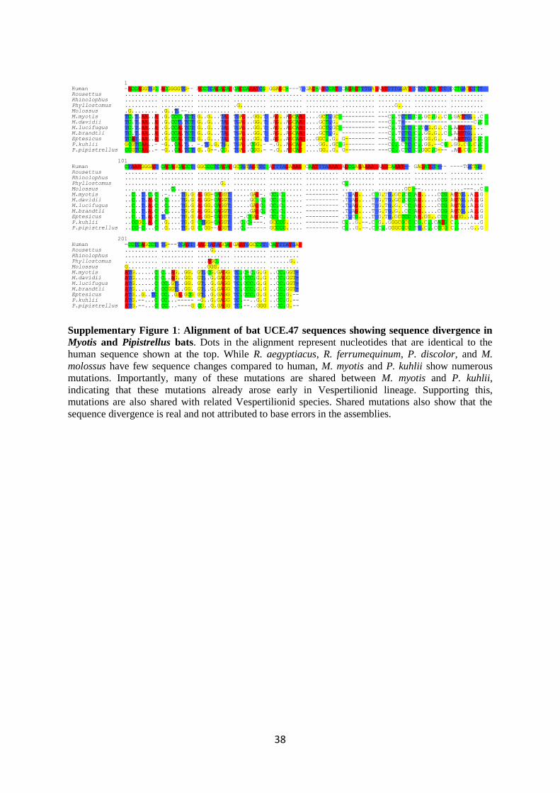
38

Supplementary Figure 1: Alignment of bat UCE.47 sequences showing sequence divergence in

Myotis and Pipistrellus bats. Dots in the alignment represent nucleotides that are identical to the

human sequence shown at the top. While R. aegyptiacus, R. ferrumequinum, P. discolor, and M.

molossus have few sequence changes compared to human, M. myotis and P. kuhlii show numerous

mutations. Importantly, many of these mutations are shared between M. myotis and P. kuhlii,

indicating that these mutations already arose early in Vespertilionid lineage. Supporting this,

mutations are also shared with related Vespertilionid species. Shared mutations also show that the

sequence divergence is real and not attributed to base errors in the assemblies.

1

Human -ACCAGGTGC ACGGGGTG-- ACCTCACACA CACCAAATCG GGAGC----T GAC-ATCCAT CACACTTTGA AATTTTGGAT TTCATCATTT CCTGATCTTTRousettus .......... .......... .......... .......... .......... .......... .......... .......... .......... ..........Rhinolophus .......... .......... .......... .......... .......... .......... .......... .......... .......... ..........

Phyllostomus .......... .......... .......... .G........ .......... .......... .......... .....G.... .......... ..........Molossus .G........ .G..T.--.. .......... .......... .......... .......... .......... .......... .......... ..........M.myotis TC.T.AA..A .G.CCC.TCT G..G...TA. TGA...GG.T .AG..AGCAA ....GCT.GC ---------- ---C..TCTC C..GC.G..C .GATTG...C

M.davidii TC.T.AA..A .G.CCT.TCT G..G...TA. TGA...GG.T .AG..AGCAA ....GCT.G. ---------- ---C..T--- ---------- -------C.CM.lucifugus TC.T.AA..A .G.CCA.TCT G..G...TA. TGA...GG.T .AG..AGCAA ....GCT.GC ---------- ---C..TCTC C.TGG.G..C .AATTG....M.brandtii TC.T.AA..A .G.CCA.TCT G..G...TA. TGA...GG.T .AG..AGCAA ....GCT.G. ---------- ---C..TCTC C..GG.G..C .AATTG....

Eptesicus TCAT.AA..A .G.CCA.TCT G..G...TA. TGA...GG.T .AG..AGCAA ...GGC..G. G--------- ---C..TCTC C..GG.G... .AATTG.C.CP.kuhlii GCGTCAA..- -G..CA.T.. -.TG.G.TG. TGA..CGG.- -.G..AGCAG ....GG..GC G--------- ---CC..CTC C..GG.--CG .GG.CG.C.CP.pipistrellus CCGTCAA..- -G..CA.TCT G..G--.CG. TGA..CGG.- -.G..AGCAG ....GG..G. G--------- ---CC..CTC C.GGC.G--- .AG.CG.C.C

101Human CTAAAGGGAT CACAGCACCT GGCCCTCACA GCTGTAGTTC ATTTAGAAAG CAATTTAAAA ACCGAGAAAA AAGCAAAT-- GACATCT--- ----TGCTG-

Rousettus .......... .......... .......... .......... .......... .......... .......... .......... .......... ..........Rhinolophus .......... .......... .......... .......... .......... .......... .......... .......... .......... ..........Phyllostomus .......... .......... .......G.. .......... .......... .......... C......... .......... .......... ..........

Molossus .......... ...C...... .......... .......... .......... .......... .......... ........GC --........ ....---..CM.myotis ..C..T.C.C .-....TG.G A.GG-CAGGT .....GA.-. CC.C...... ---------- .T.AG....C G.TG.GC.CC AG.....CCG AGTG..A..GM.davidii ..C..T.A.C .C....TG.G A.GG-CAGGT .....GC.C. CC.C...... ---------- .T.AG....T G.TG.GC.CC AG.....CCG AGTG..A..G

M.lucifugus ..C..T.A.C .C....TG.G A.GG.CAGGT .....GA.C. CC.C...... ---------- .T.AG....T G.TG.G..CC AG.....CCG AGTG..A..GM.brandtii ..C..T.A.C .C....TG.G A.GG.CAGGT .....GA.C. CC.C...... ---------- .T.AG....T G.TG.G..CC AG.....CCG AGTG..A..GEptesicus ..C..T.A.C T.....TG.G A.GG-CAGGT ..-.CGA.-. CC.C...... ---------- .T.CG....T G.TG.GCCCC AG.GG..CCG AGGG..A..G

P.kuhlii ..CCGC.A.C .G....TG.G CTGG-CAGGT ..C.C----. GCCCG..... ---------- C...G.--.C G..GGGCGCC CG.C..CACG C........GP.pipistrellus ..CC-C...C .G....TG.G C.GG--AGGT ..C.------ GCCCG..... ---------- C...G.--.C C..GGGCGCC TG.C..CGCG C.....G..G

201Human -CCTCAGCCT TG---TCATT AAGTATAGCA GAATGGCCTT CATTTATGARousettus .......... .......... ....G..... .......... .........

Rhinolophus .......... .......... .......... .......... .........Phyllostomus .......... .......... ...AGC.... .......... ......G..Molossus G......... .......... ...GGG.... .......... .........

M.myotis ATG......C C..AG..GG. GT.CG.GAGG TC.C-C.G.G ..CC.GGT-M.davidii ATG......C C..AG..GG. GT..G.GAGG TC.CCC.G.G ..CC.GGT-M.lucifugus ATG......C CC.GT..GG. GT..G.GAGG TC.CCC.G.G ..CC.GGT-

M.brandtii ATG......C CCGGT..GG. GT..G.GAGG TC.CCC.G.G ..CC.GGT-Eptesicus ATG..G..TC CC..GA.GCG GT..G.GAGG TC.CCC.G.G ..CC.G.--P.kuhlii ATG.--...C CC...----- -G..G.GAGG TC.--..G.G ..CC.G.--

P.pipistrellus ATG.--...C CC...----G CG..G.GAGG TC.--..GGG ..CC.G.--

39

Supplementary Figure 2: Genetic distance of Vespertilionid UCE.47 to other bats and canonical

human sequence. The heatmap shows that the UCE.47 sequences of Rousettus, Rhinolophus,

Phyllostomus, Molossus and human are highly conserved. In contrast, the sequence of Vespertilionid

bats, represented by Myotis, Eptesicus and Pipistrellus species, is substantially diverged from the

conserved UCE sequence but relatively similar within the clade.

40

Supplementary Figure 3: Alignment of bat UCE.394 sequences showing sequence divergence in

Pipistrellus bats. Dots in the alignment represent nucleotides that are identical to the human sequence

shown at the top. Compared to other bats, P. kuhlii shows an increased number of mutations in this

UCE sequence. These mutations are supported by Illumina reads (note that reads do not cover the

entire UCE locus). Furthermore, most mutations are shared with P. pipistrellus (which has two nearly

identical loci in the current genome assembly), indicating that the sequence divergence is real and not

attributed to base errors in the assembly.

1Human CGGCAAGGTA AATACTTTTG GAAAATAAGT GGAAATTTGC TGCAAATCAG TCCCTTTTGT GCATGGCCGC GGGAGCATGT TGAAATGTTTRousettus ...T...... .......... .......... .......... .......... .......... .......... .......... ..........

Rhinolophus ...T...... .......... .......... .......... .......... .-........ .......... .......... ..........

Phyllostomus ...T...... .......... .......... .......... .......... .......... ..G....... .......... ..........Molossus .......... .G........ .......... .......... .......... .......... ..C....... A......... ..........

Myotis ...G...... ..C....... .......... .......... .......... .......... .......... .......... ..........P._pipistrellus_locus_1 ...A...... .......... .......... .......... C......... C......... ..GC.....G ......G... ..........P._pipistrellus_locus_2 ...A...... .......... .......... .......... C......... C......... ..GC.....G ......G... ..........

P._kuhlii ...A...... .......... .......... .......... C......... C......... ..GC.....G ......G... ..........2218:0:437514365 ---------- ---------- .......... .......... C......... C......... ..GC.....G ......G... ..........1219:0:200095769 ---------- ---------- ---------- ---------- ---------- ---------- ---------- -------GT. C.........

2105:0:262043991 ---------- ---------- ---....... .......... C......... C......... ..GC.....G ......G... ..........1217:0:191913956 ---------- -------... .......... .......... C......... C......... ..GC.....G ......G... ..........1202:0:125676924 ---------- ---------- ---------- -.G..A.... C......... C......... ..GC.....G ......G... ..........

2110:0:280385277 ---------- ---------- ---------- ---------- ---------- ---------- ---------- ----..G... ..........1206:0:142783782 ---------- ---------- ---------- ---------- ---------- ------.... ..GC.....G ......G... ..........1125:0:104801572 ---------- ---------- ---------- ---------- ---------- ---------- --GC.....G ......G... ..........

1119:0:77880338 ---------- ---------- ---------- ---------- ---------- ---------- ---------- ......G... ..........1220:0:206019745 ---------- ---------- ---------- ---------- ---------- ---------- ---------- --------.. ..........1103:0:9981575 ---------- ---------- ---------- ---------- ---------- ---------- ---------- ---------- ----------

2213:0:415474342 ---------- ---------- ---------- ---------- ---------- ---------- ---------G ......C... ..........1111:0:46732173 ---------- ---------- ---------- ---------- ---------- ---------- ---------- ---------. ..........2225:0:469014465 ---------- ---------- ---------- ---------- ---------- ---------- ---------- ---------- ----------

2225:0:468965810 ---------- ---------- ---------- ---------- ---------- ---------- ---------- ---------- ----------

2119:0:323272794 ---------- ---------- ---------- ---------- ---------- ---------- ---------- ---------- ----------2119:0:323268082 ---------- ---------- ---------- ---------- ---------- ---------- ---------- ---------- ----------

1110:0:42758830 ---------- ---------- -----..... .......... C......... C......... ..GC.....G ......G... ..........1227:0:236630582 ---------- ---------- ---------- ---------- ---------- ---------- ---------- ----..G... ..........2202:0:369450373 ---------- ---------- ---------- ---------- ---------- -----..... ..GC.....G ......G... ..........

1115:0:60493502 ----...... .......... .......... .......... C......... C......... ..GC.....G ......G... ..........1119:0:81422856 ---------- ---------- ---------- ---------- ---------- ---....G.. ..GC.....G ......G... ..........1115:0:62606794 ---------- ---------- ---------- ---------- ---------- ------.... ..GC.....G ......G... ..........

2101:0:244763915 ---------- ---------- ---------- ---------- ---------- ---------- ---------- -----.G... ..........2219:0:443440196 ---------- ---------- ---------- ---------- ---------- ---------- ---------- ---------- ----------2212:0:411628431 ---------- ---------- ---------- ---------- ---------- ---------- ---------- ---------- ----------

2101:0:244760776 ---------- ---------- ---------- ---------- ---------- ---------- ---------- ------G... ..GG.....G1113:0:54413129 ---------- ---------- ---------- ---------- ---------- ---------- ---------- ---------- ---------.

91Human GGACACTAAT ACCCATTCAT TT-TCTTGGC -TCCATAAAT AAAAGCCGCC AGCTCTGTGG CGGCCGTGAA ATGGTATTCT TC-AGGGCCCRousettus .......... .......... .......... .......... ......T... .......... .T........ ...T....T. ....A...T.

Rhinolophus .......... .......... .......... .......... .......... .......... .......... .......... ..........Phyllostomus .......... .......... .......... .......... .....A.... G..A...... T......C.. .......... ...-......

Molossus .......... .......... .......... .......... .........T ....TG.... .......C.. .......... .T.G....T.

Myotis .......... .......... .......... .......... ........G. C..A.C.... ......CC.. ....C..... ...G......P._pipistrellus_locus_1 .......... T......... ...C.CC... T...C..... .......... C....G.... .A...ACC.. ....C..... C..C......P._pipistrellus_locus_2 .......... T......... ..CC.CC... T...C..... ......T... C....G.... .A...ACC.. ....C..... C..C......

P._kuhlii .......... T......... .....CC... T...C..... ....------ --------.. .A....CC.. ....C..... C..G......2218:0:437514365 .......... T......... .....CC... T...C..... ....------ --------.. .A....CC.. ....C..... --.-------1219:0:200095769 .......... T......... .....CC... T...C..... ....------ --------.. .A....CC.. ....C..... C..G......

2105:0:262043991 .......... T......... .....CC... T...C..... ....------ --------.. .A....CC.. ....C..... C..G------1217:0:191913956 .........- T......... .....CC... T...C..... ....------ --------.. .A....CC.. ....C...-- --.-------1202:0:125676924 .......... T......... .....CC... T...C..... ....------ --------.. .A....CC.. ....C..... C..G------

2110:0:280385277 .......... T......... ...-.CC... T...C..... ....------ --------.. .A....CC.. ....C..... C..G......

1206:0:142783782 .......... T......... .....CC... T...C..... ....------ --------.. .A....CC.. ....C..... C..G......1125:0:104801572 .......... T......... ...G.CC... T...C..... ....------ --------.. .A....CC.. ....C..... C..G......

1119:0:77880338 .......... T......... .....CC... T...C..... ....------ --------.. .A....CC.. ....C..... C..G......1220:0:206019745 .......... T......... .....CC... T...C..... ....------ --------.. .A....CC.. ....C..... C..G......1103:0:9981575 -------... T......... .....CC... T...C..... ....------ --------.. .A....CC.. ....C..... C..G......

2213:0:415474342 .......... T......... .....CC... T...C..... ....------ --------.. .A....CC.. ....C..... C..G......1111:0:46732173 .......... T......... .....CC... T...C..... ....------ --------.. .A....CC.. ....C..... C..G......2225:0:469014465 -----..... T......... .....CC... T...C..... ....------ --------.. .A....CC.. ....C..... C..G......

2225:0:468965810 -----..... T......... .....CC... T...C..... ....------ --------.. .A....CC.. ....C..... C..G......2119:0:323272794 -----..... T......... .....CC... T...C..... ....------ --------.. .A....CC.. ....C..... C..G......2119:0:323268082 -----..... T......... ...C.CC... T...C..... ....------ --------.. .A....CC.. ....C..... C..G......

1110:0:42758830 .......... T......... .....CC... T...C..... ....------ --------.. .A....CC.. ....C....- --.-------1227:0:236630582 .......... T......... ...-.CC... T...C..... ....------ --------.. .A....CC.. ....C..... C..G......2202:0:369450373 .......... T......... .....CC... T...C..... ....------ --------.. .A....CC.. ....C..... C..G......

1115:0:60493502 .......... T......... .....CC... T...C..... ....------ --------.. .A....CC.. ....C...-- --.-------1119:0:81422856 .......... T......... .....CC... T...C..... ....------ --------.. .A....CC.. ....C..... C..G......1115:0:62606794 .......... T......... .....CC... T...C..... ....------ --------.. .A....CC.. ....C..... C..G......

2101:0:244763915 .......... T......... .....CC... T...C..... ....------ --------.. .A....CC.. ....C..... C..G......2219:0:443440196 .......... T......... .....CC... T...C..... ....------ --------.. .A....CC.. ....C..... C..G......2212:0:411628431 -----...C. T......... .....CC... T...C..... ....------ --------.. .A....CC.. ....C..... C..G......

2101:0:244760776 ....G.G... G...G..... .....CC... G...C..... ....------ --------.. .A....CC.. ....C..... C..G......

1113:0:54413129 ........GA T......... ...G.CC... TG..CA.... ....------ --------.. .A....CC.. ....C..... C.GG......

181Human AGC--AGGAA CCCCCATCCT TATT-ACC

Rousettus .....T.... .T.T.G.... ....C...

Rhinolophus .......... ..T....... ........Phyllostomus .....-..G. A....C.... C.......Molossus ........GT .....C.... ........

Myotis .....-..GG G....C.T.. ........P._pipistrellus_locus_1 .....G..GG GA...C.T.. ........P._pipistrellus_locus_2 .....G..GG GA...C.T.. ........

P._kuhlii .....G..GG GA...C.T.. ........2218:0:437514365 ---..----- ---------- ----.---1219:0:200095769 .....G..GG GA...C.T.. ........

2105:0:262043991 ---..----- ---------- ----.---

1217:0:191913956 ---..----- ---------- ----.---1202:0:125676924 ---..----- ---------- ----.---

2110:0:280385277 .....G..GG GA...C.T.. ........1206:0:142783782 ...GGG..GG GA...C.T.. ........1125:0:104801572 .....G..GG GA...C.T.. ........

1119:0:77880338 .....G..GG GA...C.T.. ........1220:0:206019745 .....G..GG GA...C.T.. ........1103:0:9981575 .....G..GG GA...C.T.. ........

2213:0:415474342 .....G..GG GA...C.T.. ........1111:0:46732173 .....G..GG GA...C.T.. ........2225:0:469014465 .....G..GG GA...C.T.. ........

2225:0:468965810 .....G..GG GA...C.T.. ........2119:0:323272794 .....G..GG GA...C.T.. ........2119:0:323268082 .....G..GG GA...C.T.. ........

1110:0:42758830 ---..----- ---------- ----.---1227:0:236630582 .....G..GG GA...C.T.. ........2202:0:369450373 .....G..GG GA-------- ----.---

1115:0:60493502 ---..----- ---------- ----.---1119:0:81422856 .....G..GG GA...C.T.. ........1115:0:62606794 ...GGG..GG GA...C.T.. ........

2101:0:244763915 .....G..GG GA...C.T.. ........

2219:0:443440196 .....G..GG GA...C.T.. ........2212:0:411628431 .....G..GG GA...C.T.. ........

2101:0:244760776 .....G..GG GA...C.T.. ........1113:0:54413129 .....G..GG GA...C.T.. ........

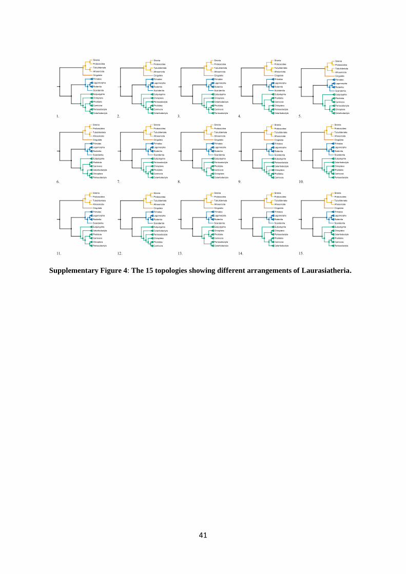
41

Supplementary Figure 4: The 15 topologies showing different arrangements of Laurasiatheria.

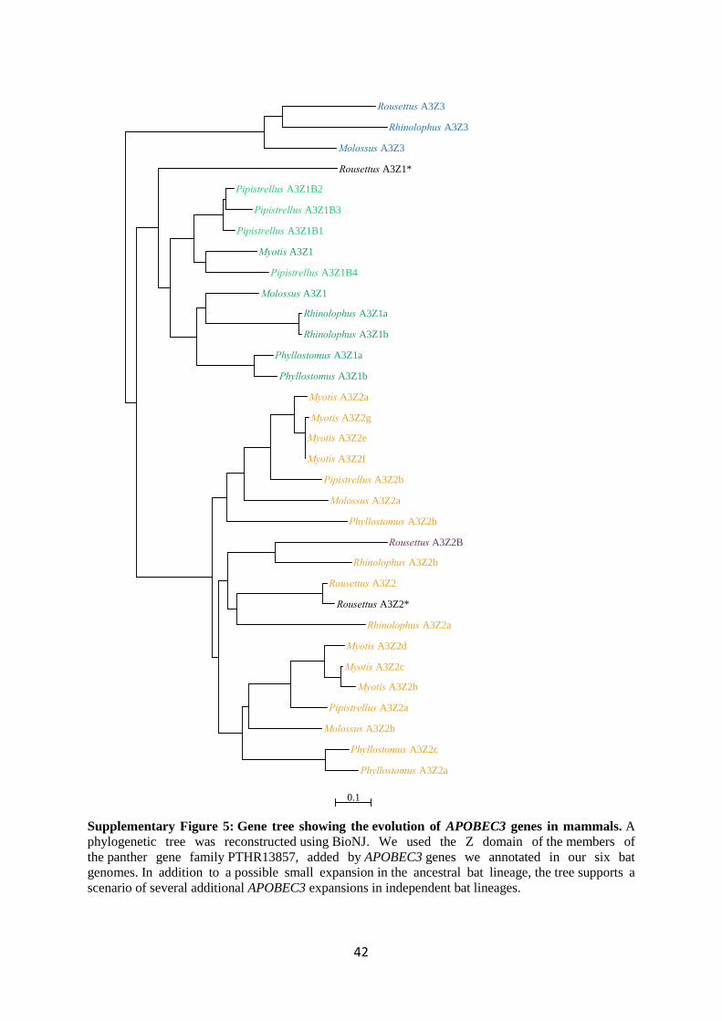
42

Supplementary Figure 5: Gene tree showing the evolution of APOBEC3 genes in mammals. A

phylogenetic tree was reconstructed using BioNJ. We used the Z domain of the members of

the panther gene family PTHR13857, added by APOBEC3 genes we annotated in our six bat

genomes. In addition to a possible small expansion in the ancestral bat lineage, the tree supports a

scenario of several additional APOBEC3 expansions in independent bat lineages.

Phyllostomus A3Z2a

Phyllostomus A3Z2c

Molossus A3Z2b

Pipistrellus A3Z2a

Myotis A3Z2b

Myotis A3Z2c

Myotis A3Z2d

Rhinolophus A3Z2a

Rousettus A3Z2*

Rousettus A3Z2

Rhinolophus A3Z2b

Rousettus A3Z2B

Phyllostomus A3Z2b

Molossus A3Z2a

Pipistrellus A3Z2b

Myotis A3Z2f

Myotis A3Z2e

Myotis A3Z2g

Myotis A3Z2a

Phyllostomus A3Z1b

Phyllostomus A3Z1a

Rhinolophus A3Z1b

Rhinolophus A3Z1a

Molossus A3Z1

Pipistrellus A3Z1B4

Myotis A3Z1

Pipistrellus A3Z1B1

Pipistrellus A3Z1B3

Pipistrellus A3Z1B2

Rousettus A3Z1*

Molossus A3Z3

Rhinolophus A3Z3

Rousettus A3Z3

0.1

43

Supplementary Figure 6: Mosaic plot showing the relative numbers of viral gene sequences

found in six bat genomes compared to seven mammalian reference genomes.

44

Supplementary Figure 7: Reconstructed phylogenetic tree of viral pol sequences found in six

species of bats. Each species used in the ERV search is marked with a colour: Phyllostomus (navy

blue), Myotis (green), Pipistrellus (orange), Rhinolophus (yellow), Molossus (light blue), Rousettus

(pink) and reference sequences (black). Bootstrap values are shown where the values are ≥ 70%. The

tips of the phylogeny are labelled with the species name, position in the reference genomes and the

direction of the sequences (N- negative/P- positive).

(See Separate File for Supplementary Figure 7)

45

Supplementary Figure 8: The number of conserved noncoding RNA genes shared across 6 bat

species. The figure was generated using UpSetR149

. Each black dot indicates each species. The

connected black dots indicate the number of noncoding RNA genes shared between them.

7 6 4 4 2 2 2 2 1 1 1 1 114

4 2 2 2 1 1 1 1 1 115 8 8 7 3 3

479

0

200

400

Nu

mb

er

of

ncR

NA

Rousettus

Rhinolophus

Phyllostomus

Molossus

Pipistrellus

Myotis

0200400

Number of ncRNA

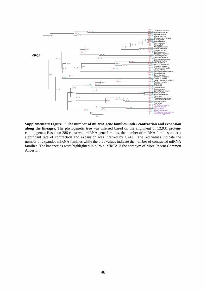
46

Supplementary Figure 9: The number of miRNA gene families under contraction and expansion

along the lineages. The phylogenetic tree was inferred based on the alignment of 12,931 protein-

coding genes. Based on 286 conserved miRNA gene families, the number of miRNA families under a

significant rate of contraction and expansion was inferred by CAFE. The red values indicate the

number of expanded miRNA families while the blue values indicate the number of contracted miRNA

families. The bat species were highlighted in purple. MRCA is the acronym of Most Recent Common

Ancestor.

47

Supplementary Figure 10: The performance of the Dollo parsimony principle on random and

real data. The real data refer to the observed phylogenetic tree inferred from the alignment of 12,931

protein-coding genes and the matrix containing the number of miRNA copies across 48 mammalian

species; while the random data refer to the relationship of species in the phylogenetic tree and the

number of miRNA copies that have been randomly shuffled. The figure indicates the number of losses

required to explain the observed phylogenetic pattern, both on real and random data.

0.00

0.05

0.10

0.15

0 10 20

Number of losses required

Fre

qu

ency

of

miR

NA

gen

e fa

mily

Real data

Random data

48

Supplementary Figure 11: The miRNA gene loss and acquisition based on the Dollo parsimony

principle. The red numbers indicate miRNA gain while the blue numbers indicate miRNA loss. The

bat species were highlighted in purple.

49

Supplementary Figure 12: The evolution of novel miRNA predicted in 6 bat species. a) The

number of novel mature miRNA shared across 6 bat species. b) The number of novel seeds shared

across 6 bat species.

248

234

215209

126117

5 4 3 2 2 1 1 1 1 1 1 10

100

200

Nu

mb

er

of

sha

red m

atu

re n

ove

l m

iRN

A

Rousettus

Rhinolophus

Phyllostomus

Molossus

Pipistrellus

Myotis

0100200

Number of novel miRNA

225

163

150149

8980

1811 9 9 9 8 7 6 6 5 4 3 3 2 1 4 3 3 3 2 2 1 1 1 1 1 1

0

50

100

150

200

250

Nu

mb

er

of

novel se

ed

s

Rousettus

Rhinolophus

Phyllostomus

Molossus

Pipistrellus

Myotis

050100150200250

Number of novel miRNA

a b

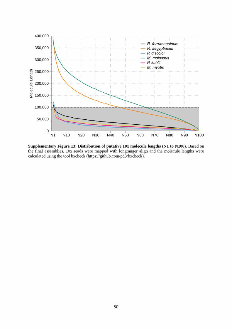
50

Supplementary Figure 13: Distribution of putative 10x molecule lengths (N1 to N100). Based on

the final assemblies, 10x reads were mapped with longranger align and the molecule lengths were

calculated using the tool bxcheck (https://github.com/pd3/bxcheck).

R. ferrumequinum

R. aegyptiacus

P. discolor

M. molossus

P. kuhlii

M. myotis

Mole

cu

le L

en

gth

0

50,000

100,000

150,000

200,000

250,000

300,000

350,000

400,000

N1 N10 N20 N30 N40 N50 N60 N70 N80 N90 N100

51

Supplementary Figure 14: The tree topology inferred with a supermatrix of 12,931 genes.

Divergence times are calculated using the tree topology inferred with a supermatrix of 12,931 genes.

Node calibrated with fossils are highlighted in red.

102030405060708090100 0

Trichechus manatus

Loxodonta africana

Orycteropus afer

Echinops telfairi

Dasypus novemcinctus

Gorilla gorilla

Homo sapiens

Pan troglodytes

Pongo abelii

Macaca fascicularis

Saimiri boliviensis

Calllithrix jacchus

Carlito syrichta

Microcebus murinus

Otolemur garnettii

Rattus norvegicus

Mus musculus

Microtus ochrogaster

Cricetulus griseus

Heterocephalus glaber

Cavia porcellus

Ictidomys tridecemlineatus

Ochotona princeps

Oryctolagus cuniculus

Tupaia belangeri

Sorex araneus

Erinaceus europaeus

Condylura cristata

Balaenoptera acutoristrata

Tursiops truncatus

Bos taurus

Sus scrofa

Camelus ferus

Equus caballus

Ceratotherium simum

Manis javanica

Manis pentadactyla

Leptonychotes weddellii

Mustela putorius

Ailuropoda melanoleuca

Canis lupus

Felis catus

Pipistrellus kuhlii

Myotis myotis

Molossus molossus

Phyllostomus discolor

Rhinolophus ferrumequinum

Rousettus aegyptiacus

Divergence Times (Mya)

52

Supplementary Figure 15: Genes under positive selection on Carnivora and Cetartiodactyla

branches (a) Genes showing evidence of significant positive selection after multiple test correction

across both aBSREL (12,821 genes) and codeml (2,436 genes) for Carnivora are shown. Genes not in

the candidate 2,453 genes that were significant in HyPhy and subsequently validated with codeml are

designated by ‘*’. (b) Genes showing evidence of significant positive selection across both aBSREL

(12,866 genes) and codeml (2,443 genes) for Cetartiodactyla are displayed.

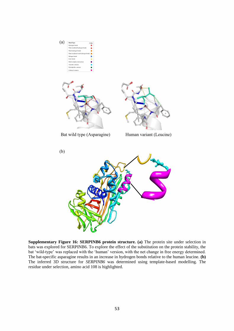
53

Supplementary Figure 16: SERPINB6 protein structure. (a) The protein site under selection in

bats was explored for SERPINB6. To explore the effect of the substitution on the protein stability, the

bat ‘wild-type’ was replaced with the ‘human’ version, with the net change in free energy determined.

The bat-specific asparagine results in an increase in hydrogen bonds relative to the human leucine. (b)

The inferred 3D structure for SERPINB6 was determined using template-based modelling. The

residue under selection, amino acid 108 is highlighted.

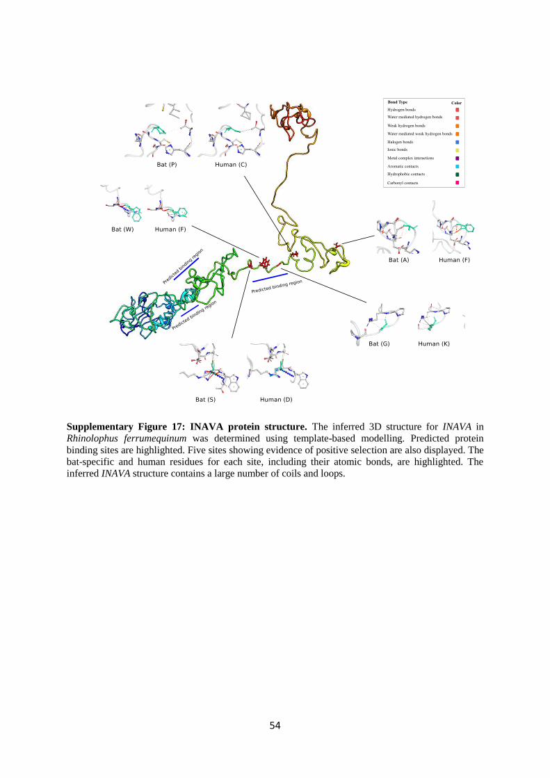
54

Supplementary Figure 17: INAVA protein structure. The inferred 3D structure for INAVA in

Rhinolophus ferrumequinum was determined using template-based modelling. Predicted protein

binding sites are highlighted. Five sites showing evidence of positive selection are also displayed. The

bat-specific and human residues for each site, including their atomic bonds, are highlighted. The

inferred INAVA structure contains a large number of coils and loops.

55

Supplementary Figure 18: Loss of PYHIN genes in bats. UCSC genome browser screenshot shows

the PYHIN genes in the human genome (blue highlight). The alignment nets show that all six bats

have large deletions that remove these genes, which is consistent with previous results that all bats

have lost these genes130

. Because these genes are also lost in several other mammals, we filtered them

out in our genome-wide screen for gene losses.

56

Supplementary Figure 19: Genomic annotation of predicted miRNA loci in 6 bat species. a) The

number of known and novel miRNA located in exonic, intronic and intergenic regions; b) The

percentage of known and novel miRNA located in exonic, intronic and intergenic regions.

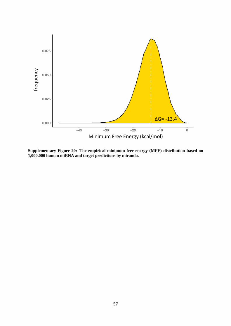
57

Supplementary Figure 20: The empirical minimum free energy (MFE) distribution based on

1,000,000 human miRNA and target predictions by miranda.

58

Supplementary Table 1: Information of 48 mammalian genomes used for comparative and

phylogenetic analyses in this study. The species highlighted in blue indicate 6 bat species whose

genomes were sequenced in this study while the species in red indicate 7 species used as references

for comparative analyses. For cow and cat, we additionally used the most recent bosTau9 and felCat9

assembly to assess completeness of BUSCO genes and UCEs.

59

Supplementary Table 2: The final genomes (all lengths in Mb). N50 values correspond to post hoc

genome size of the final assemblies (sum of the length of all scaffolds).

60

Supplementary Table 3: Manual curation and consistency with karyotypes. This table shows data

for both the non-curated and curated P. kuhlii assembly.

Species Splits / Joins# of Chromosomes

in Karyotype = N

Correlation with

top N ScaffoldsTail

Status

% of Data in N

Largest Scaffolds

M. myotis 2 / 6 21+2 0.993 Tail (18) 95.62%

P. kuhlii not curated 21+2 0.992 Tail (33) 86.54%

P. kuhlii 4 / 76 21+2 0.995 Tail (2) 97.99%

R. ferrumequinum 3 / 1 28+1 0.980 Incline (5) 98.89%

P. discolor 10 / 13 15+2 0.989 Cliff (0) 99.67%

R. aegyptiacus 0 / 5 17+2 0.995 Cliff (0) 99.85%

M. molossus 2 / 6 23+2 0.989 Incline (7) 98.52%

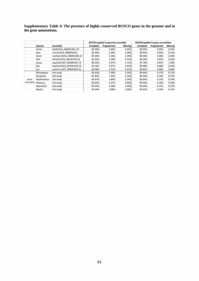
61

Supplementary Table 4: The presence of highly-conserved BUSCO genes in the genome and in

the gene annotations.

species assembly Complete Fragmented Missing Complete Fragmented Missing

Homo hg38 (GCA_000001405.27) 94.59% 2.46% 2.95% 99.95% 0.00% 0.05%

Mus mm10 (GCA_000001635) 95.30% 2.36% 2.34% 99.83% 0.02% 0.15%

Canis canFam3 (GCA_000002285.2) 95.30% 2.36% 2.34% 98.56% 1.00% 0.44%

Felis felCat9 (GCA_000181335.4) 95.30% 2.39% 2.31% 98.39% 0.97% 0.63%

Equus equCab3 (GCF_002863925.1) 96.22% 2.07% 1.71% 97.78% 0.85% 1.36%

Bos bosTau9 (GCA_002263795.2) 94.10% 2.97% 2.92% 98.98% 0.68% 0.34%

Sus susScr11 (GCF_000003025.6) 94.08% 3.51% 2.41% 98.85% 0.68% 0.46%

Rhinolophus this study 95.42% 2.36% 2.22% 99.66% 0.17% 0.17%

Rousettus this study 95.83% 1.92% 2.24% 99.34% 0.29% 0.37%

Phyllostomus this study 94.91% 1.80% 3.29% 99.66% 0.15% 0.19%

Molossus this study 92.93% 3.17% 3.90% 99.49% 0.19% 0.32%

Pipistrellus this study 95.35% 2.36% 2.29% 99.56% 0.17% 0.27%

Myotis this study 94.44% 2.88% 2.68% 99.63% 0.24% 0.12%

Bat1K

assemblies

BUSCO applied to gene annotationBUSCO applied to genome assembly

62

Supplementary Table 5: Analysis of ultraconserved elements (UCEs) that do not align with ≥ 85%

identity and at least 150 bp.

63

Supplementary Table 6: Best-fit models of sequence evolution for all coding genes, CNEs and

1st +2nd codon site alignments were determined using IQTREE.

(See separate file)

Supplementary Table 7: The metrics of the alignments of 12,931 genes.

(See separate file)

Supplementary Table 8: Results of the genome-wide screen for positive selection in coding genes.

Uncorrected P-values are calculated by using the likelihood ratio test as implemented for the aBSREL

model in HyPhy. These values are corrected using the Holm-Bonferroni correction for the number of

branches tested. The Gene-corrected P-values are produced by applying the false discovery rate

procedure over all genes tested (n=12,931) to the LRT derived p-value. The “Double-corrected” value

is the Branch-corrected p-value post FDR correction (n=12,931).

(See separate file)

Supplementary Table 9: The significant genes under positive selection along the bat ancestral

branch using PAML. The likelihood ratio test (LRT) was used to calculate p-values using a chi-

square distribution (one sided). P-values were adjusted using FDR correction (n=2,453).

(See separate file)

Supplementary Table 10: The lists of genes under positive selection on Carnivora and

Cetartiodactyla branches. The likelihood ratio tests (LRT) was used to calculate p-values using a

chi-square distribution (one sided). P-values were adjusted using FDR correction, n=2,436 and 2,443,

respectively.

(See separate file)

64

Supplementary Table 11: Genes that were inferred to be lost in all 6 bats analysed in this study.

Gene Symbol Ensembl Gene ID

AS3MT ENSG00000214435

HIST1H4K ENSG00000273542

IL36G ENSG00000136688

KLK4 ENSG00000167749

KRBA2 ENSG00000184619

LRRC70 ENSG00000186105

MS4A3 ENSG00000149516

U2AF1L4 ENSG00000161265

ZBED9 ENSG00000232040

ZFP30 ENSG00000120784

65

Supplementary Table 12: Gene families that were estimated to have undergone a contraction or

expansion in the ancestral bat lineage. Values shown are P-values calculated using the Viterbi

method as implemented in CAFE for evidence in shift in the rate of birth/death of a gene family along

the given branch. "Corrected Chiroptera" gives the Viterbi P-value after FDR correction along the

Chiroptera ancestral branch. The Family ID is the PANTHER family ID. Where multiple PANTHER

families were collapsed, IDs were concatenated. If no human protein was present in a family, no

PANTHER ID was not assigned, and an internal identifier used. Expansion/Contraction was

determined by comparing the Chiroptera ancestor to the inferred scrotiferan ancestor.

(See separate file)

Supplementary Table 13: The number of 286 conserved miRNA gene copies across 48

mammalian taxa based on the de novo genomic prediction using the Infernal pipeline.

(See separate file)

66

Supplementary Table 14: Oligonucleotide sequences used for cloning. Restriction site tags

and spacers between individual miRNA binding sites are highlighted in bold, mature

miRNAs are italic, and miRNA seed sequences are underlined.

Insert for cloning SENSE OLIGO (5’→3’) ANTISENSE OLIGO (5’→3’)

Bat-miR-19125

CTAGATCCCTTGGAAAGAGCCTTGTTTTGGAAGGGAAGGGGGAAGAGGCTCTGCC

CTTGACCTCTACCCTTTGTTTCCTTCCAGCCTTTGTCCAGGAGTTGAGGAAGAGGG

TCGACCCTCTTCCTCAACTCCTGGACAAAGGCTGGAAGGAAACAAAGGGTAGAGGTCAAGGGC

AGAGCCTCTTCCCCCTTCCCTTCCAAAACAAGGCTCTTTCCAAGGGAT

Bat-miR-4665

CTAGACCCCTACTTGCAGTTGGTCCGACGGTTGTGGGTTATTGTTAAGCTGATTAAC

ATTGTCTCCCTCCACACAACCACATTTGACTGACTTTGTATTTTGCCCTAGTCG

TCGACGACTAGGGCAAAATACAAAGTCAGTCAAATGTGGTTGTGTGGAGGGAGACAATGTTA

ATCAGCTTAACAATAACCCACAACCGTCGGACCAACTGCAAGTAGGGGT

Bat-miR-6665

CTAGAACAAAGTAGGTTAGATCTTGCCAGATTAGGTGGAGATTCTCGCAGGGGGA

GTTCAACTTCATATACCCTTGCAAGATACTCCTCTGTCTGGAAAGGTCTTCCTCTG

TCGACAGAGGAAGACCTTTCCAGACAGAGGAGTATCTTGCAAGGGTATATGAAGTTGAACTCC

CCCTGCGAGAATCTCCACCTAATCTGGCAAGATCTAACCTACTTTGTT

Bat-miR-19125_sensor TCGAGGCTGGAAGGAAACAAAGGGTAGAGAATATGCTGGAAGGAAACAAAGGGTAGAT

CTAGATCTACCCTTTGTTTCCTTCCAGCATATTCTCTACCCTTTGTTTCCTTCCAGCC

Bat-miR-4665_sensor TCGAGCTTAACAATAACCCACAAGAAT

ATCTTAACAATAACCCACAAT

CTAGATTGTGGGTTATTGTTAAGATATTCTTG

TGGGTTATTGTTAAGC

Bat-miR-6665_sensor TCGAGCCCTGCGAGAATCTCCACCTAAGAATATCCCTGCGAGAATCTCCACCTAAT

CTAGATTAGGTGGAGATTCTCGCAGGGATATTCTTAGGTGGAGATTCTCGCAGGGC

Bat-miR-337

CTAGAACAGTCAGTAAGTGGGGGGTGAGAACGGCTTCATCCAGGAGTTGATGCCC

AGTTATCCAGCGCCTAGATGATGCCTTTCTTCATCCCCTTCAAG

TCGACTTGAAGGGGATGAAGAAAGGCATCATCTAGGCGCTGGATAACTGGGCATCAACTCCTG

GATGAAGCCGTTCTCACCCCCCACTTACTGACTGTT

hsa-miR-337

CTAGAGTAGTCAGTAGTTGGGGGGTGGGAACGGCTTCATACAGGAGTTGATGCAC

AGTTATCCAGCTCCTATATGATGCCTTTCTTCATCCCCTTCAAG

TCGACTTGAAGGGGATGAAGAAAGGCATCATATAGGAGCTGGATAACTGTGCATCAACTCCTG

TATGAAGCCGTTCCCACCCCCCAACTACTGACTACT

Bat-miR-337_sensor TCGAGGAAGAAAGGCATCATCTAGGCGGAATATGAAGAAAGGCATCATCTAGGC

GT

CTAGACGCCTAGATGATGCCTTTCTTCATATTCCGCCTAGATGATGCCTTTCTTCC

hsa-miR-337_sensor

TCGAGGAAGAAAGGCATCATATAGGAG

GAATATGAAGAAAGGCATCATATAGGAGT

CTAGACTCCTATATGATGCCTTTCTTCATATTCCTCCTATATGATGCCTTTCTTCC

67

Supplementary Table 15: The statistics of 3’UTR analysis for 6 bat genomes.

Total 3UTR

Different genes with overlapped 3UTR

loci

After merging overlapped coordinates Pseudo 3UTR

M. molossus 13,671 290 11,912 8,613

M. myotis 13,263 406 11,024 8,811

P. kuhlii 6,891 182 6,372 5,612

P. discolor 15,122 476 12,196 9,030

R. ferrumequinum 7,913 226 7,194 6,346

R. aegyptiacus 16,115 327 13,394 9,519

68

Supplementary Table 16: The gene targets of human and bat miR-337 predicted by RNAhybrid

and miranda. The gene targets, which were specific to bat and human and were shared between bat

and human, are listed respectively.

(See separate file)

69

Supplementary Table 17: Summary of miRNA sequencing and analysis in 6 bat genomes. Note

that P. discolor brain includes samples of cortex, cerebellum and striatum.

Species Tissue Accession

Number

Raw reads Mapping

rate

Known

miRNA

Novel

miRNA

Myotis myotis

Brain SRR10153055 44,256,216 90.3%

329 242 Kidney SRR10153054 41,823,612 82.7% Liver SRR10153043 42,013,686 81.8%

Pipistrellus kuhlii

Brain SRR10153039 46,857,126 92.6% 258 122 Kidney SRR10153038 35,303,058 73.2%

Liver SRR10153037 39,045,247 75.0%

Molossus

molossus

Brain SRR10153042 35,168,361 93.8%

286 229 Kidney SRR10153041 44,074,092 91.6% Liver SRR10153040 36,055,759 86.5%

Phyllostomus discolor

Brain SRR10153046 SRR10153047 SRR10153048

107,798,649 94.7% 284 133

Kidney SRR10153045 39,805,199 91.7% Liver SRR10153044 27,597,872 89.9%

Rhinolophus

ferrumequinum

Brain SRR10153036 52,426,146 91.8% 332 261 Kidney SRR10153053 50,908,913 91.1%

Liver SRR10153052 48,450,654 86.2%

Rousettus aegyptiacus

Brain SRR10153051 25,458,780 91.6%

325 217 Kidney SRR10153050 45,673,617 91.6% Liver SRR10153049 33,831,764 91.0%

70

Supplementary Table 18: The summary of 12 novel miRNA at the ancestral bat lineage. These

newly-evolved miRNAs were not found in any other species.

(See separate file)

71

Supplementary Table 19: Overview of species and tissues used for high molecular weight

genomic DNA (HMW gDNA) extraction.

Species Sex Provided by Year of collection Location

Molossus

molossus male Dina Dechmann 2018

Gamboa, Panama

(9.1165° N, 79.6965° W)

Myotis

myotis female

Emma Teeling &

Sébastien Puechmaille

2015 Limerzel, France

(47.6333° N, 2.3500° W)

Pipistrellus

kuhlii male

Emma Teeling &

Andrea Locatelli 2017

Bergamo, Italy

(45.7430° N, 9.5831° E)

Phyllostomus

discolor male Sonja Vernes 2016

Munich, Germany

(Captive colony)

Rhinolophus ferrumequinum

female Gareth Jones 2016 United Kingdom

(51.7108° N, 2.2776° W)

Rousettus

aegyptiacus male Sonja Vernes 2017

Berkeley, USA

(Captive colony)

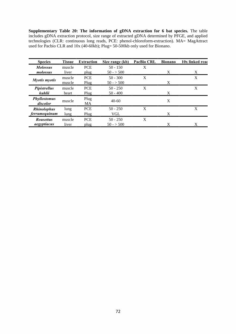
72

Supplementary Table 20: The information of gDNA extraction for 6 bat species. The table

includes gDNA extraction protocol, size range of extracted gDNA determined by PFGE, and applied

technologies (CLR: continuous long reads, PCE: phenol-chloroform-extraction). MA= MagAttract

used for Pacbio CLR and 10x (40-60kb); Plug= 50-500kb only used for Bionano.

Species Tissue Extraction Size range (kb) PacBio CRL Bionano 10x linked reads

Molossus

molossus

muscle PCE 50 - 150 X

liver plug 50 - > 500 X X

Myotis myotis muscle PCE 50 - 300 X X

muscle Plug 50 - > 500 X

Pipistrellus

kuhlii

muscle PCE 50 - 250 X X

heart Plug 50 - 400 X

Phyllostomus

discolor muscle

Plug

MA 40-60 X

Rhinolophus ferrumequinum

lung PCE 50 - 250 X X

lung Plug VGL X

Rousettus aegyptiacus

muscle PCE 50 - 250 X

liver plug 50 - > 500 X X

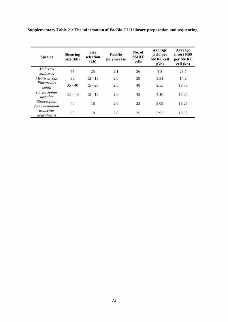
73

Supplementary Table 21: The information of PacBio CLR library preparation and sequencing.

Species Shearing

size (kb)

Size

selection (kb)

PacBio

polymerase

No. of

SMRT cells

Average yield per

SMRT cell

(Gb)

Average insert N50

per SMRT

cell (kb)

Molossus

molossus 75 25 2.1 26 4.8 23.7

Myotis myotis 35 12 - 15 2.0 39 3.31 14.3 Pipistrellus

kuhlii 35 - 40 15 - 20 2.0 48 2.55 13.76

Phyllostomus discolor

35 - 40 12 - 15 2.0 43 4.10 15.05

Rhinolophus

ferrumequinum 40 18 2.0 25 5.09 18.25

Rousettus

aegyptiacus 60 18 2.0 35 3.92 18.08

74

Supplementary Table 22: Sequencing depth, effective genome coverage and mean molecular

length calculated by the 10x Supernova tool.

Species Long

gDNA megasize

gDNA

Sequenced

fragments (Mi reads)

Genome

coverage (linked reads)

Mean

molecular length (kb)

Molossus

molossus - X 354 49x 131.9

Myotis myotis X - 319 44x 29.4 Pipistrellus

kuhlii X - 327 46x 19.7

Phyllostomus

discolor X - 789 109x 16.0

Rhinolophus ferrumequinum

X - 345 48x 28.8

Rousettus

aegyptiacus - X 365 51 97.9

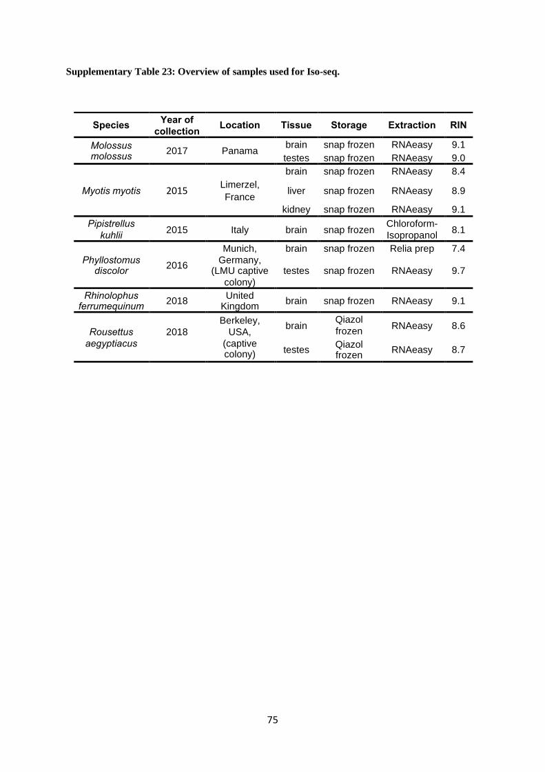
75

Supplementary Table 23: Overview of samples used for Iso-seq.

Species Year of

collection Location Tissue Storage Extraction RIN

Molossus molossus

2017 Panama brain snap frozen RNAeasy 9.1 testes snap frozen RNAeasy 9.0

Myotis myotis

brain snap frozen RNAeasy 8.4

2015 Limerzel,

France liver snap frozen RNAeasy 8.9

kidney snap frozen RNAeasy 9.1

Pipistrellus

kuhlii 2015 Italy brain snap frozen

Chloroform-

Isopropanol 8.1

Phyllostomus discolor

2016

Munich,

Germany, (LMU captive

colony)

brain snap frozen Relia prep 7.4

testes snap frozen RNAeasy 9.7

Rhinolophus ferrumequinum

2018 United Kingdom brain snap frozen RNAeasy 9.1

Rousettus

aegyptiacus

2018

Berkeley,

USA,

(captive colony)

brain Qiazol

frozen RNAeasy 8.6

testes Qiazol frozen

RNAeasy 8.7

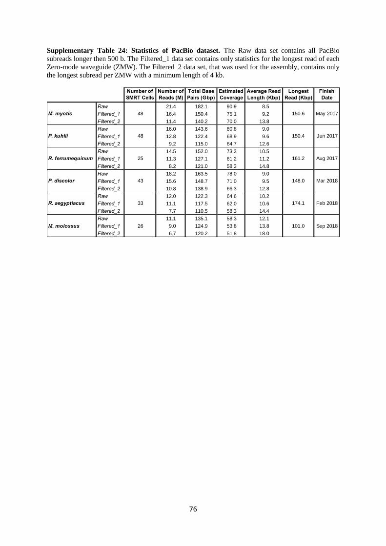
76

Supplementary Table 24: Statistics of PacBio dataset. The Raw data set contains all PacBio

subreads longer then 500 b. The Filtered_1 data set contains only statistics for the longest read of each

Zero-mode waveguide (ZMW). The Filtered_2 data set, that was used for the assembly, contains only

the longest subread per ZMW with a minimum length of 4 kb.

Number of

SMRT Cells

Number of

Reads (M)

Total Base

Pairs (Gbp)

Estimated

Coverage

Average Read

Length (Kbp)

Longest

Read (Kbp)

Finish

Date

Raw 21.4 182.1 90.9 8.5

Filtered_1 16.4 150.4 75.1 9.2

Filtered_2 11.4 140.2 70.0 13.8

Raw 16.0 143.6 80.8 9.0

Filtered_1 12.8 122.4 68.9 9.6

Filtered_2 9.2 115.0 64.7 12.6

Raw 14.5 152.0 73.3 10.5

Filtered_1 11.3 127.1 61.2 11.2

Filtered_2 8.2 121.0 58.3 14.8

Raw 18.2 163.5 78.0 9.0

Filtered_1 15.6 148.7 71.0 9.5

Filtered_2 10.8 138.9 66.3 12.8

Raw 12.0 122.3 64.6 10.2

Filtered_1 11.1 117.5 62.0 10.6

Filtered_2 7.7 110.5 58.3 14.4

Raw 11.1 135.1 58.3 12.1

Filtered_1 9.0 124.9 53.8 13.8

Filtered_2 6.7 120.2 51.8 18.0

26

M. myotis

P. kuhlii

R. ferrumequinum

P. discolor

R. aegyptiacus

M. molossus

48

48

25

43

33

May 2017

101.0

174.1

148.0

161.2

150.4

150.6

Sep 2018

Feb 2018

Mar 2018

Aug 2017

Jun 2017

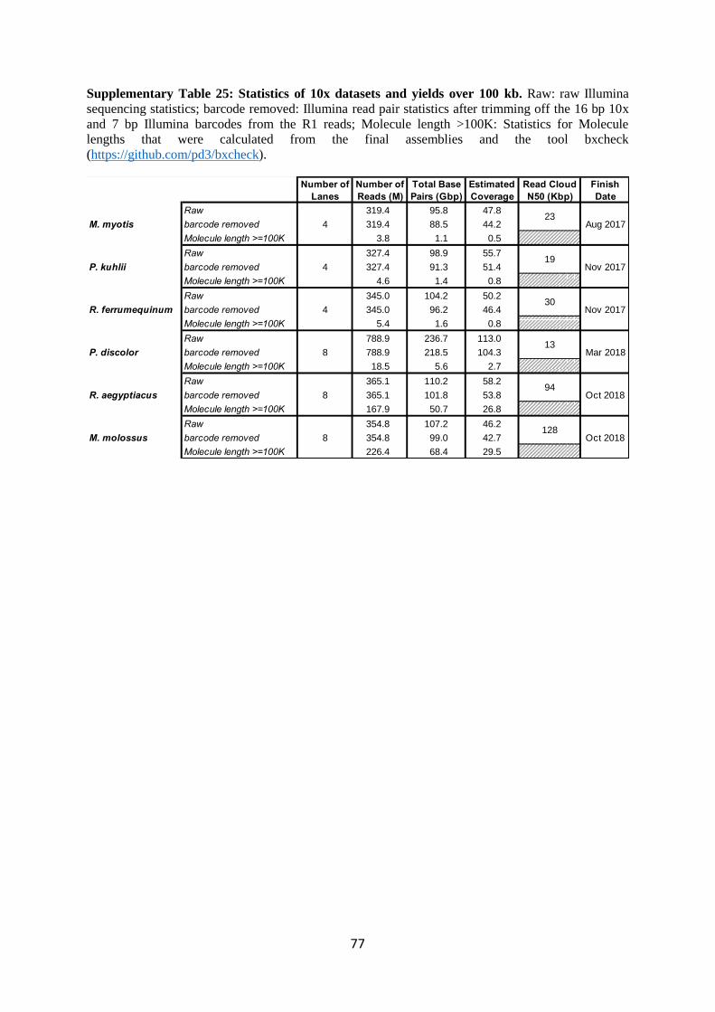
77

Supplementary Table 25: Statistics of 10x datasets and yields over 100 kb. Raw: raw Illumina

sequencing statistics; barcode removed: Illumina read pair statistics after trimming off the 16 bp 10x

and 7 bp Illumina barcodes from the R1 reads; Molecule length >100K: Statistics for Molecule

lengths that were calculated from the final assemblies and the tool bxcheck

(https://github.com/pd3/bxcheck).

Number of

Lanes

Number of

Reads (M)

Total Base

Pairs (Gbp)

Estimated

Coverage

Read Cloud

N50 (Kbp)

Finish

Date

Raw 319.4 95.8 47.8

barcode removed 319.4 88.5 44.2

Molecule length >=100K 3.8 1.1 0.5

Raw 327.4 98.9 55.7

barcode removed 327.4 91.3 51.4

Molecule length >=100K 4.6 1.4 0.8

Raw 345.0 104.2 50.2

barcode removed 345.0 96.2 46.4

Molecule length >=100K 5.4 1.6 0.8

Raw 788.9 236.7 113.0

barcode removed 788.9 218.5 104.3

Molecule length >=100K 18.5 5.6 2.7

Raw 365.1 110.2 58.2

barcode removed 365.1 101.8 53.8

Molecule length >=100K 167.9 50.7 26.8

Raw 354.8 107.2 46.2

barcode removed 354.8 99.0 42.7

Molecule length >=100K 226.4 68.4 29.5

R. aegyptiacus 8 Oct 2018

M. molossus 8 Oct 2018128

94

R. ferrumequinum 4 Nov 2017

P. discolor 8 Mar 201813

30

M. myotis 4 Aug 2017

P. kuhlii 4 Nov 2017

23

19

78

Supplementary Table 26: Statistics of Bionano dataset. The filtered data set were used for the de

novo Bionano assembly and consists of molecules with a minimum length of 150 kb and a minimum

of 9 label sites.

Technology Number of

Molecules (M)

Total Length

(Gbp)

Estimated

Coverage

Average Molecule

Length (Kbp)

Finish Date

Where

Raw 27.7 1960 979 71 Nov 2018

Filtered 2.0 396 198 195 Ploen

Raw 17.9 1419 799 79 Nov 2018

Filtered 1.9 460 259 242 Ploen

Raw 6.4 547 263 85 Dec 2017

Filtered 1.0 313 151 308 Rockefeller

Raw 12.0 1046 504 89 Dec 2017

Filtered 2.1 597 288 286 Rockefeller

Raw 6.7 764 365 114 Jun 2017

Filtered 1.8 480 229 265 Rockefeller

Raw 2.7 315 150 118 Jun 2017

Filtered 0.7 186 89 151 Rockefeller

Raw 2.4 410 216 169 Feb 2019

Filtered 1.0 320 169 309 Dresden

Raw 9.2 948 409 102 Oct 2017

Filtered 2.0 462 199 234 Ploen

R. aegyptiacus

M. molossus

DLE1

DLE1

P. discolor

BSPQI

BSSSI

BSPQI

BSSSI

M. myotis

P. kuhlii

DLE1

DLE1

R. ferrumequinum

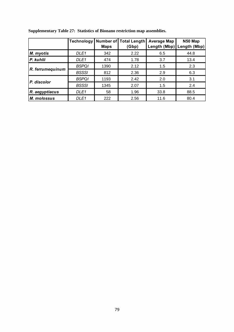
79

Supplementary Table 27: Statistics of Bionano restriction map assemblies.

Technology Number of

Maps

Total Length

(Gbp)

Average Map

Length (Mbp)

N50 Map

Length (Mbp)

M. myotis DLE1 342 2.22 6.5 44.8

P. kuhlii DLE1 474 1.78 3.7 13.4

BSPQI 1390 2.12 1.5 2.3

BSSSI 812 2.36 2.9 6.3

BSPQI 1193 2.42 2.0 3.1

BSSSI 1345 2.07 1.5 2.4

R. aegyptiacus DLE1 58 1.96 33.8 88.5

M. molossus DLE1 222 2.56 11.6 80.4

P. discolor

R. ferrumequinum

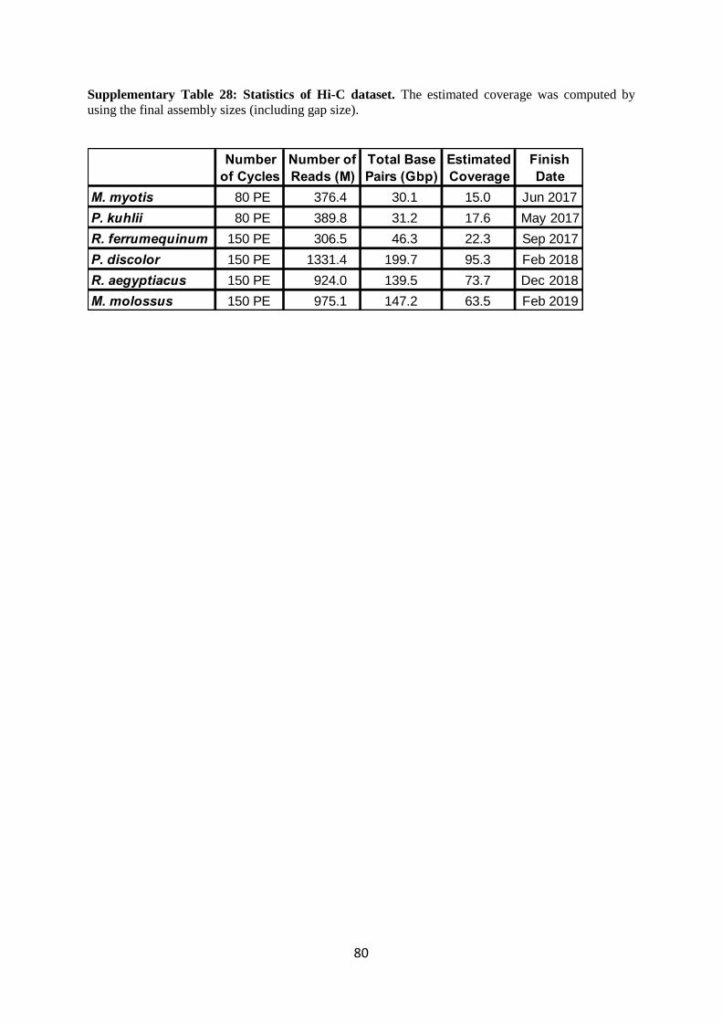
80

Supplementary Table 28: Statistics of Hi-C dataset. The estimated coverage was computed by

using the final assembly sizes (including gap size).

Number

of Cycles

Number of

Reads (M)

Total Base

Pairs (Gbp)

Estimated

Coverage

Finish

Date

M. myotis 80 PE 376.4 30.1 15.0 Jun 2017

P. kuhlii 80 PE 389.8 31.2 17.6 May 2017

R. ferrumequinum 150 PE 306.5 46.3 22.3 Sep 2017

P. discolor 150 PE 1331.4 199.7 95.3 Feb 2018

R. aegyptiacus 150 PE 924.0 139.5 73.7 Dec 2018

M. molossus 150 PE 975.1 147.2 63.5 Feb 2019

81

Supplementary Table 29: The genomes after read assembly. (all lengths in Mb, NG50 correspond

to post hoc genome size of the final assemblies.)

NumberTotal

LengthNG50 Number

Total

LengthN50 Number

Total

LengthN50

M. myotis 598 1,976 11.80 671 55 0.10 406 22 0.06

P. kuhlii 527 1,765 10.24 624 53 0.10 270 13 0.05

R. ferrumequinum 324 2,056 21.74 67 58 0.10 120 7 0.07

P. discolor 421 2,056 16.15 234 20 0.10 245 14 0.06

R. aegyptiacus 260 1,866 21.74 108 10 0.11 141 9 0.07

M. molossus 396 2,261 21.58 565 89 0.18 205 15 0.08

Species

Primary Contigs Alternate Contigs Discarded Contigs

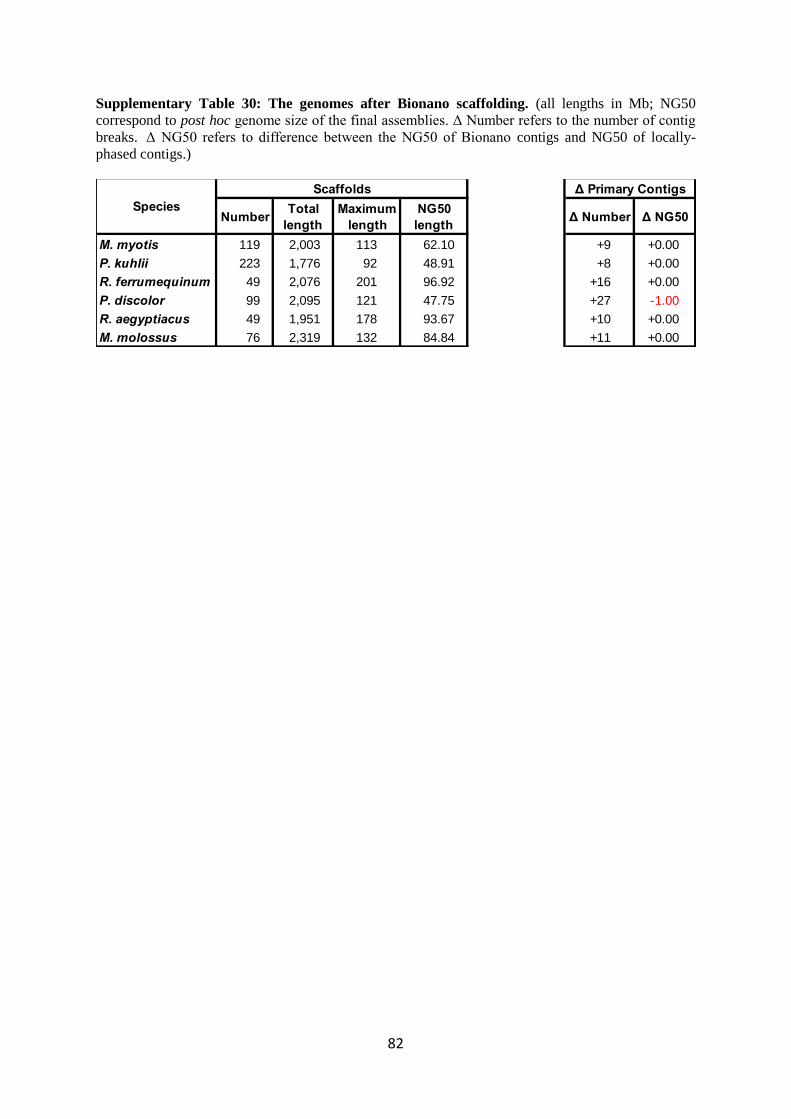
82

Supplementary Table 30: The genomes after Bionano scaffolding. (all lengths in Mb; NG50

correspond to post hoc genome size of the final assemblies. Δ Number refers to the number of contig

breaks. Δ NG50 refers to difference between the NG50 of Bionano contigs and NG50 of locally-

phased contigs.)

NumberTotal

length

Maximum

length

NG50

lengthΔ Number Δ NG50

M. myotis 119 2,003 113 62.10 +9 +0.00

P. kuhlii 223 1,776 92 48.91 +8 +0.00

R. ferrumequinum 49 2,076 201 96.92 +16 +0.00

P. discolor 99 2,095 121 47.75 +27 -1.00

R. aegyptiacus 49 1,951 178 93.67 +10 +0.00

M. molossus 76 2,319 132 84.84 +11 +0.00

Species

Scaffolds Δ Primary Contigs

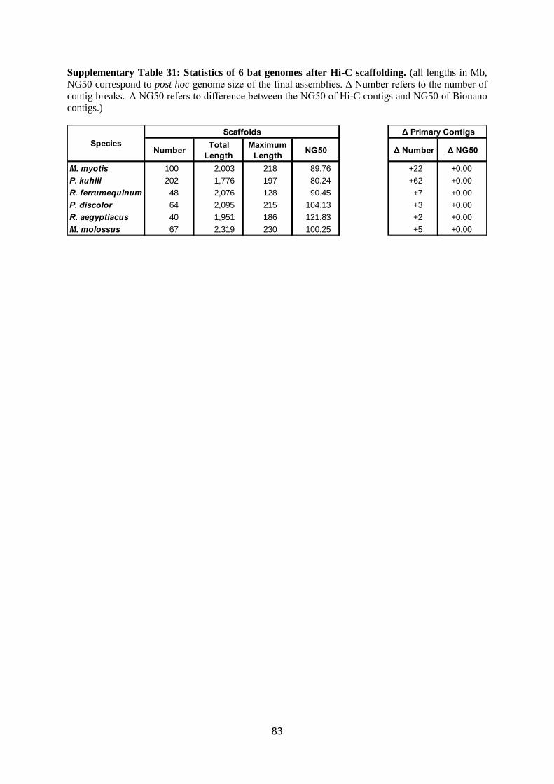
83

Supplementary Table 31: Statistics of 6 bat genomes after Hi-C scaffolding. (all lengths in Mb,

NG50 correspond to post hoc genome size of the final assemblies. Δ Number refers to the number of

contig breaks. Δ NG50 refers to difference between the NG50 of Hi-C contigs and NG50 of Bionano

contigs.)

NumberTotal

Length

Maximum

LengthNG50 Δ Number Δ NG50

M. myotis 100 2,003 218 89.76 +22 +0.00

P. kuhlii 202 1,776 197 80.24 +62 +0.00

R. ferrumequinum 48 2,076 128 90.45 +7 +0.00

P. discolor 64 2,095 215 104.13 +3 +0.00

R. aegyptiacus 40 1,951 186 121.83 +2 +0.00

M. molossus 67 2,319 230 100.25 +5 +0.00

Species

Scaffolds Δ Primary Contigs

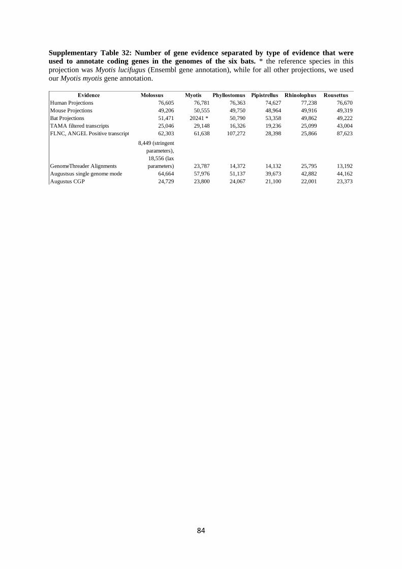
84

Supplementary Table 32: Number of gene evidence separated by type of evidence that were

used to annotate coding genes in the genomes of the six bats. * the reference species in this

projection was Myotis lucifugus (Ensembl gene annotation), while for all other projections, we used

our Myotis myotis gene annotation.

Evidence Molossus Myotis Phyllostomus Pipistrellus Rhinolophus Rousettus

Human Projections 76,605 76,781 76,363 74,627 77,238 76,670

Mouse Projections 49,206 50,555 49,750 48,964 49,916 49,319

Bat Projections 51,471 20241 * 50,790 53,358 49,862 49,222

TAMA filtered transcripts 25,046 29,148 16,326 19,236 25,099 43,004

FLNC, ANGEL Positive transcripts 62,303 61,638 107,272 28,398 25,866 87,623

GenomeThreader Alignments

8,449 (stringent

parameters),

18,556 (lax

parameters) 23,787 14,372 14,132 25,795 13,192

Augustsus single genome mode 64,664 57,976 51,137 39,673 42,882 44,162

Augustus CGP 24,729 23,800 24,067 21,100 22,001 23,373

85

Supplementary Table 33: Related species used for Genome Threader alignments. Details of

publicly available cDNA and protein data aligned to 6 genome assemblies for annotation from a

related species.

Reference species Query species Query source No. of query cDNA No. of query peptides Related at taxonomic rank

Molossus molossus Miniopterus natalensis Refseq 25,266 25,266 Superfamily: Vespertilionoidea

Myotis myotis Myotis lucifugus Ensembl 22,432 20,719 Genus: Myotis

Phyllostomus discolor Desmodus rotundus Refseq 28,829 28,829 Family: Phyllostomidae

Pipistrellus kuhlli Eptesicus fuscus Refseq 18,724 18,263 Subfamily: Vespertilioninae

Rhinolophus ferrumequinum Rhinolophus sinicus Refseq 29,785 29,785 Genus: Rhinolophus

Rousettus aegyptiacus Pteropus vampyrus Ensembl 18,086 17,053 Subamily: Pteropodinae

86

Supplementary Table 34: Sources of RNA-Seq and Iso-seq transcriptomic data that we used for

annotating genes.

Species Tissue Accession Number/ Bioproject

Brain SRR11528221

Heart SRR11528219; SRR11528220

Liver SRR11528217; SRR11528218

Kidney SRR11528215; SRR11528216

Molossus molossus Blood SRR11526509 - SRR11526516

Phyllostomus discolor Brain PRJNA291690

Pipistrellus kuhlii Fibroblast PRJNA565655

Brain SRR1048140

Brain SRR1048142

Liver SRR2754983

Liver SRR2757329

Intestine SRR6749599

Intestine SRR6749600

Intestine SRR6749601

Intestine SRR6749602

Testes SRR2914372

Liver SRR2914369

Kidney SRR2914360

Heart SRR2914359

Brain SRR2914295

Liver SRR2914059

Kidney SRR2913355

Heart SRR2913354

Brain SRR2913353

Myotis myotis

Rhinolophus ferrumequinum

Rousettus aegyptiacus

87

Supplementary Table 35: Base pair counts and genome proportion estimates of transposable

element classes in each examined taxon.

(See separate file)

Supplementary Table 36: The library of viral protein sequences used for endogenous viral

elements (EVE) analysis.

(See separate file)

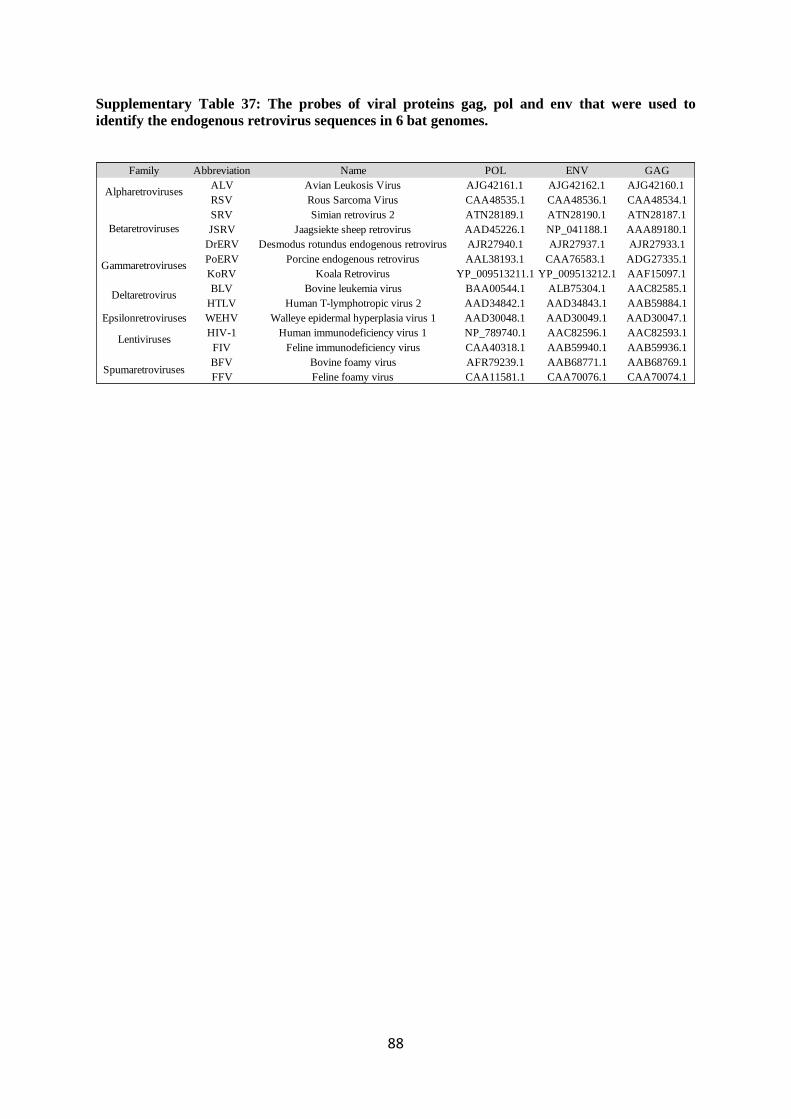
88

Supplementary Table 37: The probes of viral proteins gag, pol and env that were used to

identify the endogenous retrovirus sequences in 6 bat genomes.

Family Abbreviation Name POL ENV GAG

ALV Avian Leukosis Virus AJG42161.1 AJG42162.1 AJG42160.1

RSV Rous Sarcoma Virus CAA48535.1 CAA48536.1 CAA48534.1

SRV Simian retrovirus 2 ATN28189.1 ATN28190.1 ATN28187.1

JSRV Jaagsiekte sheep retrovirus AAD45226.1 NP_041188.1 AAA89180.1

DrERV Desmodus rotundus endogenous retrovirus AJR27940.1 AJR27937.1 AJR27933.1

PoERV Porcine endogenous retrovirus AAL38193.1 CAA76583.1 ADG27335.1

KoRV Koala Retrovirus YP_009513211.1 YP_009513212.1 AAF15097.1

BLV Bovine leukemia virus BAA00544.1 ALB75304.1 AAC82585.1

HTLV Human T-lymphotropic virus 2 AAD34842.1 AAD34843.1 AAB59884.1

Epsilonretroviruses WEHV Walleye epidermal hyperplasia virus 1 AAD30048.1 AAD30049.1 AAD30047.1

HIV-1 Human immunodeficiency virus 1 NP_789740.1 AAC82596.1 AAC82593.1

FIV Feline immunodeficiency virus CAA40318.1 AAB59940.1 AAB59936.1

BFV Bovine foamy virus AFR79239.1 AAB68771.1 AAB68769.1

FFV Feline foamy virus CAA11581.1 CAA70076.1 CAA70074.1Spumaretroviruses

Alpharetroviruses

Betaretroviruses

Gammaretroviruses

Deltaretrovirus

Lentiviruses

89

Supplementary Table 38: The Number of viral integrations in analysed genomes. The number of

all retroviral integrations found in six bat genomes for each viral class and protein (Pol, Gag, Env).

Pol sequences were additionally searched in seven reference genomes and their numbers were

compared.

(See separate file)

90

Supplementary Table 39: Divergence time estimates (in millions of years) using r8s. Their

respective nodes are relative to tree topology 1.

Node Divergence

Time (Mya) Eutherian Root 99.37

Atlantogenata 93.26

Afrotheria 71.7

Paenungulata 59.2

Tubulidentata+Afrosoricida 68.91

Boreoeutheria 94.67

Euarchontoglires 82.85

Primates 66

Haplorhini 61.26

Simiiformes 29.21

Catarrhini 20.55

Hominidae 10

Homininae 5.73

Pan+Homo 5.11

Saimiri+Callithrix 12.93

Strepsirrhini 48.84

Glires 81.85

Rodentia+Lagomorpha 78.81

Lagomorpha 50.76

Rodentia 66

Hystricomorpha 64.86

Muroidea 34.86

Murinae 21.61

Microtus+Cricetulus 28.24

Heterocephalidae+Caviidae 37.41

Laurasiatheria 88.14

Eulipotyphla 82.45

Erinaceidae+Soricidae 76.85

Scrotifera 77.26

Carnivora+Pholidota+Cetartiodactyla+Perissodactyla 74.67

Cetartiodactyla+Perissodactyla 73.13

Cetartiodactyla 55.86

Sus+Bos+Cetacea 52.74

Bos+Cetacea 47.51

Cetacea 34

Perissodactyla 55.5

Carnivora+Pholidota 69.9

Pholidota 8.03

Carnivora 43

Caniformia 34.64

Arctoidea 27.12

Leptonychotes+Mustela 25.53

Chrioptera 63.39

Yangochiroptera 52.79

Molossus+Vespertilionidae 47.39

Vespertilionidae 24.7

Yinpterochiroptera 56.64

91

Supplementary Table 40: The 15 topologies showing different arrangements of Laurasiatheria

and the number of gene trees supporting them with the highest likelihood. Positions of other

mammals are fixed relative to the coding-gene supermatrix topology (topology 1).

(See separate file)

Supplementary Table 41: The name, alignment length and number of taxa present for 10,857

conserved non-coding elements (CNEs).

(See separate file)

Supplementary Table 42: RF distances between all gene trees.

(See separate file)

Supplementary Table 43: All 2,453 genes relating to ageing/immunity/metabolism used in

selection analysis with PAML and their taxonomic representation.

(See separate file)

Supplementary Table 44: Protein structure prediction of the genes under positive selection in

bats.

(See separate file)

Supplementary Table 45: The miRNA families that were gained and lost in the bat lineages.

(See separate file)

Supplementary Table 46: Investigation of conserved one-to-one single-copy miRNA genes in 6

bat species compared to other 42 mammalian taxa. The conservation of mature miRNA and their

seed regions was manually curated. 5p and 3p indicate the coordinates of 5p & 3p mature miRNA in

multiple alignments. The empirical expression data were based on miRBase (release 22). The missing

values indicate that the miRNA does not have either 5p or 3p mature sequences.

(See separate file)

Supplementary Data File 1: De novo curated transposable elements combined with a vertebrate

library of known TEs in RepBase.

(See separate file)

Supplementary Data File 2: Alignments of 12,931 protein-coding genes across 48 mammals.

(See separate file)

Supplementary Data File 3: Predicted 3D protein structures of candidate genes.

(See separate file)

92

References

1 Teeling, E. C. et al. A molecular phylogeny for bats illuminates biogeography and the fossil

record. Science 307, 580-584 (2005).

2 Teeling, E. C. et al. Bat Biology, Genomes, and the Bat1K Project: To Generate

Chromosome-Level Genomes for All Living Bat Species. Annu Rev Anim Biosci 6, 23-46

(2018).

3 A reference standard for genome biology. Nat Biotechnol 36, 1121 (2018).

4 Kitzman, J. O. Haplotypes drop by drop. Nat Biotechnol 34, 296-298 (2016).

5 Mostovoy, Y. et al. A hybrid approach for de novo human genome sequence assembly and

phasing. Nat Methods 13, 587-590 (2016).

6 Nowoshilow, S. et al. The axolotl genome and the evolution of key tissue formation

regulators. Nature 554, 50-55 (2018).

7 Grohme, M. A. et al. The genome of Schmidtea mediterranea and the evolution of core

cellular mechanisms. Nature 554, 56-61 (2018).

8 Myers, E. W. The Dresden AZZembLER for long read projects. Available

at:https://dazzlerblog.wordpress.com/.

9 Tischler, G. & Myers, E. W. Non hybrid long read consensus using local de Bruijn graph

assembly. bioRxiv, 106252 (2017).

10 Tischler, G. Haplotype and repeat separation in long reads. bioRxiv, 145474 (2017).

11 Myers, E. W. Detecting and Masking Repeats, Available at:

https://dazzlerblog.wordpress.com/2016/04/01/detecting-and-soft-masking-repeats/.

12 Garrison, E. M., G. . Haplotype-based variant detection from short-read sequencing. arXiv,

arXiv:1207.3907 (2012).

13 Kerpedjiev, P. et al. HiGlass: web-based visual exploration and analysis of genome

interaction maps. Genome Biol 19, 125 (2018).

14 Li, H. & Durbin, R. Fast and accurate short read alignment with Burrows-Wheeler transform.

Bioinformatics 25, 1754-1760 (2009).

15 Ghurye, J., Pop, M., Koren, S., Bickhart, D. & Chin, C. S. Scaffolding of long read

assemblies using long range contact information. BMC Genomics 18, 527 (2017).

16 Bradnam, K. R. et al. Assemblathon 2: evaluating de novo methods of genome assembly in

three vertebrate species. GigaScience 2, 10 (2013).

17 Koren, S. et al. De novo assembly of haplotype-resolved genomes with trio binning. Nat

Biotechnol 36, 1174-1182 (2018).

18 Rhie, A. et al. Towards complete and error-free genome assemblies of all vertebrate species.

bioRxiv. doi: https://doi.org/10.1101/2020.05.22.110833 (2020).

19 Kent, W. J., Baertsch, R., Hinrichs, A., Miller, W. & Haussler, D. Evolution's cauldron:

duplication, deletion, and rearrangement in the mouse and human genomes. Proc Natl Acad

Sci U S A 100, 11484-11489 (2003).

20 Sharma, V., Schwede, P. & Hiller, M. CESAR 2.0 substantially improves speed and accuracy

of comparative gene annotation. Bioinformatics 33, 3985-3987 (2017).

21 Gremme, G., Brendel, V., Sparks, M. E. & Kurtz, S. Engineering a software tool for gene

structure prediction in higher organisms. Information and Software Technology 47, 965-978

(2005).

22 Kim, D., Langmead, B. & Salzberg, S. L. HISAT: a fast spliced aligner with low memory

requirements. Nat Methods 12, 357-360 (2015).

23 Li, H. et al. The Sequence Alignment/Map format and SAMtools. Bioinformatics 25, 2078-

2079 (2009).

24 Pertea, M. et al. StringTie enables improved reconstruction of a transcriptome from RNA-seq

reads. Nat Biotechnol 33, 290-295 (2015).

25 Camacho, C. et al. BLAST+: architecture and applications. BMC Bioinformatics 10, 421

(2009).

93

26 Colombo, M., Karousis, E. D., Bourquin, J., Bruggmann, R. & Muhlemann, O.

Transcriptome-wide identification of NMD-targeted human mRNAs reveals extensive

redundancy between SMG6- and SMG7-mediated degradation pathways. RNA 23, 189-201

(2017).

27 Stanke, M., Schoffmann, O., Morgenstern, B. & Waack, S. Gene prediction in eukaryotes

with a generalized hidden Markov model that uses hints from external sources. BMC

Bioinformatics 7, 62 (2006).

28 Hoff, K. J., Lomsadze, A., Borodovsky, M. & Stanke, M. Whole-Genome Annotation with

BRAKER. Methods Mol Biol 1962, 65-95 (2019).

29 Haas, B. J. et al. Automated eukaryotic gene structure annotation using EVidenceModeler

and the Program to Assemble Spliced Alignments. Genome Biol 9, R7 (2008).

30 Rodriguez, J. M. et al. APPRIS 2017: principal isoforms for multiple gene sets. Nucleic acids

Res 46, D213-D217 (2018).

31 Waterhouse, R. M. et al. BUSCO applications from quality assessments to gene prediction

and phylogenomics. Mol Biol Evol 35, 543-548 (2017).

32 Bejerano, G. et al. Ultraconserved elements in the human genome. Science 304, 1321-1325

(2004).

33 Kent, W. J. BLAT--the BLAST-like alignment tool. Genome Res 12, 656-664 (2002).

34 Hecker, N. & Hiller, M. A genome alignment of 120 mammals highlights ultraconserved

element variability and placenta-associated enhancers. GigaScience 9, giz159 (2020).

35 Platt, R. N., 2nd, Blanco-Berdugo, L. & Ray, D. A. Accurate Transposable Element

Annotation Is Vital When Analyzing New Genome Assemblies. Genome Biol Evol 8, 403-

410 (2016).

36 Smit, A., Hubley, R. & Green, P. RepeatMasker Open-4.0. 2013-2015. Available at:

http://www.repeatmasker.org.

37 Kumar, S. & Subramanian, S. Mutation rates in mammalian genomes. Proc Natl Acad Sci U S

A 99, 803-808 (2002).

38 Edgar, R. C. MUSCLE: multiple sequence alignment with high accuracy and high throughput.

Nucleic Acid Res 32, 1792-1797 (2004).

39 Capella-Gutierrez, S., Silla-Martinez, J. M. & Gabaldon, T. trimAl: a tool for automated

alignment trimming in large-scale phylogenetic analyses. Bioinformatics 25, 1972-1973

(2009).

40 Rice, P., Longden, I. & Bleasby, A. EMBOSS: the European Molecular Biology Open

Software Suite. Trends Genet 16, 276-277 (2000).

41 Abrusan, G., Grundmann, N., DeMester, L. & Makalowski, W. TEclass--a tool for automated

classification of unknown eukaryotic transposable elements. Bioinformatics 25, 1329-1330

(2009).

42 Fu, L., Niu, B., Zhu, Z., Wu, S. & Li, W. CD-HIT: accelerated for clustering the next-

generation sequencing data. Bioinformatics 28, 3150-3152 (2012).

43 Li, W. & Godzik, A. Cd-hit: a fast program for clustering and comparing large sets of protein

or nucleotide sequences. Bioinformatics 22, 1658-1659 (2006).

44 Wicker, T. et al. A unified classification system for eukaryotic transposable elements. Nat

Rev Genet 8, 973-982 (2007).

45 Pace, J. K., 2nd & Feschotte, C. The evolutionary history of human DNA transposons:

evidence for intense activity in the primate lineage. Genome Res 17, 422-432 (2007).

46 Platt, R. N., 2nd, Mangum, S. F. & Ray, D. A. Pinpointing the vesper bat transposon

revolution using the Miniopterus natalensis genome. Mob DNA 7, 12 (2016).

47 Altschul, S. F., Gish, W., Miller, W., Myers, E. W. & Lipman, D. J. Basic local alignment

search tool. J Mol Biol 215, 403-410 (1990).

48 Katzourakis, A. & Gifford, R. J. Endogenous viral elements in animal genomes. PLoS Genet

6, e1001191 (2010).

49 Larsson, A. AliView: a fast and lightweight alignment viewer and editor for large datasets.

Bioinformatics 30, 3276-3278 (2014).

50 Abascal, F., Zardoya, R. & Posada, D. ProtTest: selection of best-fit models of protein

evolution. Bioinformatics 21, 2104-2105 (2005).

94

51 Stamatakis, A. RAxML version 8: a tool for phylogenetic analysis and post-analysis of large

phylogenies. Bioinformatics 30, 1312-1313 (2014).

52 Taylor, D. J., Dittmar, K., Ballinger, M. J. & Bruenn, J. A. Evolutionary maintenance of

filovirus-like genes in bat genomes. BMC Evol Biol 11, 336 (2011).

53 Hayward, A., Grabherr, M. & Jern, P. Broad-scale phylogenomics provides insights into

retrovirus-host evolution. Proc Natl Acad Sci U S A 110, 20146-20151 (2013).

54 Skirmuntt, E. C. & Katzourakis, A. The evolution of endogenous retroviral envelope genes in

bats and their potential contribution to host biology. Virus Res 270, 197645 (2019).

55 Xu, X., Zhao, H., Gong, Z. & Han, G. Z. Endogenous retroviruses of non-avian/mammalian

vertebrates illuminate diversity and deep history of retroviruses. PLoS Patholog 14, e1007072

(2018).

56 Katzourakis, A., Tristem, M., Pybus, O. G. & Gifford, R. J. Discovery and analysis of the first

endogenous lentivirus. Proc Natl Acad Sci U S A 104, 6261-6265 (2007).

57 Farkasova, H. et al. Discovery of an endogenous Deltaretrovirus in the genome of long-

fingered bats (Chiroptera: Miniopteridae). Proc Natl Acad Sci U S A 114, 3145-3150 (2017).

58 Katzourakis, A., Gifford, R. J., Tristem, M., Gilbert, M. T. & Pybus, O. G. Macroevolution of

complex retroviruses. Science 325, 1512 (2009).

59 Wu, Z. et al. Virome analysis for identification of novel mammalian viruses in bat species

from Chinese provinces. J Virol 86, 10999-11012 (2012).

60 Katzourakis, A. et al. Larger mammalian body size leads to lower retroviral activity. PLoS

Pathog 10, e1004214 (2014).

61 Hron, T. et al. Remnants of an Ancient Deltaretrovirus in the Genomes of Horseshoe Bats

(Rhinolophidae). Viruses 10, 185 (2018).

62 Ranwez, V., Douzery, E. J. P., Cambon, C., Chantret, N. & Delsuc, F. MACSE v2: Toolkit

for the Alignment of Coding Sequences Accounting for Frameshifts and Stop Codons. Mol

Biol Evol 35, 2582-2584 (2018).

63 Kalyaanamoorthy, S., Minh, B. Q., Wong, T. K. F., von Haeseler, A. & Jermiin, L. S.

ModelFinder: fast model selection for accurate phylogenetic estimates. Nat Methods 14, 587-

589 (2017).

64 Nguyen, L. T., Schmidt, H. A., von Haeseler, A. & Minh, B. Q. IQ-TREE: a fast and effective

stochastic algorithm for estimating maximum-likelihood phylogenies. Mol Biol Evol 32, 268-

274 (2015).

65 Hoang, D. T., Chernomor, O., von Haeseler, A., Minh, B. Q. & Vinh, L. S. UFBoot2:

Improving the Ultrafast Bootstrap Approximation. Mol Biol Evol 35, 518-522 (2018).

66 Sanderson, M. J. r8s: inferring absolute rates of molecular evolution and divergence times in

the absence of a molecular clock. Bioinformatics 19, 301-302 (2003).

67 Foley, N. M., Springer, M. S. & Teeling, E. C. Mammal madness: is the mammal tree of life

not yet resolved? Philos Trans R Soc Lond B Bio Sci 371, 20150140 (2016).

68 Meredith, R. W. et al. Impacts of the Cretaceous Terrestrial Revolution and KPg extinction

on mammal diversification. Science 334, 521-524 (2011).

69 Degnan, J. H. & Rosenberg, N. A. Discordance of species trees with their most likely gene

trees. PLoS Genet 2, e68 (2006).

70 Shimodaira, H. An approximately unbiased test of phylogenetic tree selection. Syst Biol 51,

492-508 (2002).

71 Springer, M. S. & Gatesy, J. An ABBA-BABA Test for Introgression Using Retroposon

Insertion Data. bioRxiv (2019).

72 Charlesworth, B. Fundamental concepts in genetics: effective population size and patterns of

molecular evolution and variation. Nat Rev Genet 10, 195-205 (2009).

73 Hobolth, A., Andersen, L. N. & Mailund, T. On computing the coalescence time density in an

isolation-with-migration model with few samples. Genetics 187, 1241-1243 (2011).

74 Jermiin, L. S., Jayaswal, V., Ababneh, F. M. & Robinson, J. Identifying Optimal Models of

Evolution. Methods Mol Biol 1525, 379-420 (2017).

75 Ho, S. Y. & Jermiin, L. Tracing the decay of the historical signal in biological sequence data.

Syst Biol 53, 623-637 (2004).

95

76 Ababneh, F., Jermiin, L. S., Ma, C. & Robinson, J. Matched-pairs tests of homogeneity with

applications to homologous nucleotide sequences. Bioinformatics 22, 1225-1231 (2006).

77 Chifman, J. & Kubatko, L. Quartet inference from SNP data under the coalescent model.

Bioinformatics 30, 3317-3324 (2014).

78 Vachaspati, P. & Warnow, T. SVDquest: Improving SVDquartets species tree estimation

using exact optimization within a constrained search space. Mol Phylogenet Evol 124, 122-

136 (2018).

79 Springer, M. S. & Gatesy, J. Delimiting Coalescence Genes (C-Genes) in Phylogenomic Data

Sets. Genes 9, 123 (2018).

80 Springer, M. S. & Gatesy, J. The gene tree delusion. Mol Phylogenet Evol 94, 1-33 (2016).

81 Scornavacca, C. & Galtier, N. Incomplete Lineage Sorting in Mammalian Phylogenomics.

Syst Biol 66, 112-120 (2017).

82 Bogdanowicz, D. & Giaro, K. Comparing Phylogenetic Trees by Matching Nodes Using the

Transfer Distance Between Partitions. J Comput Biol 24, 422-435 (2017).

83 Schliep, K. P. phangorn: phylogenetic analysis in R. Bioinformatics 27, 592-593 (2011).

84 Paradis, E., Claude, J. & Strimmer, K. APE: Analyses of Phylogenetics and Evolution in R

language. Bioinformatics 20, 289-290 (2004).

85 Smith, M. D. et al. Less is more: an adaptive branch-site random effects model for efficient

detection of episodic diversifying selection. Mol Biol Evol 32, 1342-1353 (2015).

86 Team, R. C. R: A Language and Environment for Statistical Computing R Foundation for

Statistical Computing, Vienna, Austria (2016).

87 Yang, Z. PAML 4: phylogenetic analysis by maximum likelihood. Mol Biol Evol 24, 1586-

1591 (2007).

88 Notredame, C., Higgins, D. G. & Heringa, J. T-Coffee: A novel method for fast and accurate

multiple sequence alignment. J Mol Biol 302, 205-217 (2000).

89 Mizuta, K. et al. Ultrastructural localization of megalin in the rat cochlear duct. Hear Res 129,

83-91 (1999).

90 Kantarci, S. et al. Mutations in LRP2, which encodes the multiligand receptor megalin, cause

Donnai-Barrow and facio-oculo-acoustico-renal syndromes. Nat Genet 39, 957-959 (2007).

91 Konig, O. et al. Estrogen and the inner ear: megalin knockout mice suffer progressive hearing

loss. Faseb J 22, 410-417 (2008).

92 Sirmaci, A. et al. A truncating mutation in SERPINB6 is associated with autosomal-recessive

nonsyndromic sensorineural hearing loss. Am J Hum Genet 86, 797-804 (2010).

93 Tan, J., Prakash, M. D., Kaiserman, D. & Bird, P. I. Absence of SERPINB6A causes

sensorineural hearing loss with multiple histopathologies in the mouse inner ear. Am J Pathol

183, 49-59 (2013).

94 de Magalhaes, J. P. & Toussaint, O. Telomeres and telomerase: a modern fountain of youth?

Rejuvenation Res 7, 126-133 (2004).

95 Carbon, S. et al. AmiGO: online access to ontology and annotation data. Bioinformatics 25,

288-289 (2009).

96 O'Sullivan, T. et al. Interleukin-17D mediates tumor rejection through recruitment of natural

killer cells. Cell Rep 7, 989-998 (2014).

97 Chen, Q. X. et al. Genomic variations within DEFB1 are associated with the susceptibility to

and the fatal outcome of severe sepsis in Chinese Han population. Genes Immun 8, 439-443

(2007).

98 Alturaiki, W. et al. Expression of the B cell differentiation factor BAFF and chemokine

CXCL13 in a murine model of Respiratory Syncytial Virus infection. Cytokine 110, 267-271

(2018).

99 Bao, Y. Q. et al. Increased circulating CXCL13 levels in systemic lupus erythematosus and

rheumatoid arthritis: a meta-analysis. Clin Rheumatol 39, 193-219 (2019).

100 Maleki, K. T., Cornillet, M. & Bjorkstrom, N. K. Soluble SEMA4D/CD100: A novel

immunoregulator in infectious and inflammatory diseases. Clin Rheumatol 163, 52-59 (2016).

101 Liu, Y. J. et al. TSLP: an epithelial cell cytokine that regulates T cell differentiation by

conditioning dendritic cell maturation. Annu Rev Immunol 25, 193-219 (2007).

96

102 Hase, K. et al. Uptake through glycoprotein 2 of FimH(+) bacteria by M cells initiates

mucosal immune response. Nature 462, 226-230 (2009).

103 Killick, K. E. et al. Receptor-mediated recognition of mycobacterial pathogens. Cell

Microbiol 15, 1484-1495 (2013).

104 Flo, T. H. et al. Lipocalin 2 mediates an innate immune response to bacterial infection by

sequestrating iron. Nature 432, 917-921 (2004).

105 Xu-Monette, Z. Y. et al. Clinical and Biologic Significance of MYC Genetic Mutations in De

Novo Diffuse Large B-cell Lymphoma. Clin Cancer Res 22, 3593-3605 (2016).

106 Bergemann, A. D. & Johnson, E. M. The HeLa Pur factor binds single-stranded DNA at a

specific element conserved in gene flanking regions and origins of DNA replication. Mol Cell

Biol 12, 1257-1265 (1992).

107 Foley, N. M. et al. Growing old, yet staying young: The role of telomeres in bats' exceptional

longevity. Sci Adv 4, eaao0926 (2018).

108 Huang, Z. et al. Longitudinal comparative transcriptomics reveals unique mechanisms

underlying extended healthspan in bats. Nat Ecol Evol 3, 1110-1120 (2019).

109 Castrillo, A., Joseph, S. B., Marathe, C., Mangelsdorf, D. J. & Tontonoz, P. Liver X receptor-

dependent repression of matrix metalloproteinase-9 expression in macrophages. J Biol Chem

278, 10443-10449 (2003).

110 Laurencikiene, J. & Ryden, M. Liver X receptors and fat cell metabolism. Int J Obes 36,

1494-1502 (2012).

111 Castro, L. F., Lopes-Marques, M., Goncalves, O. & Wilson, J. M. The evolution of

pepsinogen C genes in vertebrates: duplication, loss and functional diversification. PloS One

7, e32852 (2012).

112 Linsley, P. S. et al. Human B7-1 (CD80) and B7-2 (CD86) bind with similar avidities but

distinct kinetics to CD28 and CTLA-4 receptors. Immunity 1, 793-801 (1994).

113 Figenschau, S. L. et al. ICAM1 expression is induced by proinflammatory cytokines and

associated with TLS formation in aggressive breast cancer subtypes. Sci Rep 8, 11720 (2018).

114 Liu, G. et al. Characterization of the peripheral blood transcriptome and adaptive evolution of

the MHC I and TLR gene families in the wolf (Canis lupus). BMC Genomics 18, 584 (2017).

115 Borrego, F. The CD300 molecules: an emerging family of regulators of the immune system.

Blood 121, 1951-1960 (2013).

116 Schotte, R. et al. The transcription factor Spi-B is expressed in plasmacytoid DC precursors

and inhibits T-, B-, and NK-cell development. Blood 101, 1015-1023 (2003).

117 Condamine, T. et al. Tmem176B and Tmem176A are associated with the immature state of

dendritic cells. J Leukoc Biol 88, 507-515 (2010).

118 Tsuchida, T. et al. The ubiquitin ligase TRIM56 regulates innate immune responses to

intracellular double-stranded DNA. Immunity 33, 765-776 (2010).

119 Roy, A., Kucukural, A. & Zhang, Y. I-TASSER: a unified platform for automated protein

structure and function prediction. Nat Protoc 5, 725-738 (2010).

120 Yang, J. et al. The I-TASSER Suite: protein structure and function prediction. Nat Methods

12, 7-8 (2015).

121 Zheng, W. et al. LOMETS2: improved meta-threading server for fold-recognition and

structure-based function annotation for distant-homology proteins. Nucleic Acids Res 47,

W429-W436 (2019).

122 Pettersen, E. F. et al. UCSF Chimera--a visualization system for exploratory research and

analysis. J Comput Chem 25, 1605-1612 (2004).

123 Zhang, C., Freddolino, P. L. & Zhang, Y. COFACTOR: improved protein function prediction

by combining structure, sequence and protein-protein interaction information. Nucleic Acids

Res 45, W291-W299 (2017).

124 Yang, J., Roy, A. & Zhang, Y. Protein-ligand binding site recognition using complementary

binding-specific substructure comparison and sequence profile alignment. Bioinformatics 29,

2588-2595 (2013).

125 Yang, J., Roy, A. & Zhang, Y. BioLiP: a semi-manually curated database for biologically

relevant ligand-protein interactions. Nucleic Acids Res 41, D1096-D1103 (2013).

97

126 Rodrigues, C. H., Pires, D. E. & Ascher, D. B. DynaMut: predicting the impact of mutations

on protein conformation, flexibility and stability. Nucleic Acids Res 46, W350-W355 (2018).

127 Sharma, V. et al. A genomics approach reveals insights into the importance of gene losses for

mammalian adaptations. Nat Commun 9, 1215 (2018).

128 Sharma, V. & Hiller, M. Coding Exon-Structure Aware Realigner (CESAR): Utilizing

Genome Alignments for Comparative Gene Annotation. Methods Mol Biol 1962, 179-191

(2019).

129 Zerbino, D. R. et al. Ensembl 2018. Nucleic Acids Res 46, D754-D761 (2018).

130 Ahn, M., Cui, J., Irving, A. T. & Wang, L. F. Unique Loss of the PYHIN Gene Family in

Bats Amongst Mammals: Implications for Inflammasome Sensing. Sci Rep 6, 21722 (2016).

131 Han, M. V., Thomas, G. W., Lugo-Martinez, J. & Hahn, M. W. Estimating gene gain and loss

rates in the presence of error in genome assembly and annotation using CAFE 3. Mol Biol

Evol 30, 1987-1997 (2013).

132 Katoh, K. & Standley, D. M. MAFFT multiple sequence alignment software version 7:

improvements in performance and usability. Mol Biol Evol 30, 772-780 (2013).

133 Guindon, S. & Gascuel, O. A simple, fast, and accurate algorithm to estimate large

phylogenies by maximum likelihood. Syst Biol 52, 696-704 (2003).

134 LaRue, R. S. et al. Guidelines for naming nonprimate APOBEC3 genes and proteins. J Virol

83, 494-497 (2009).

135 Hayward, J. A. et al. Differential Evolution of Antiretroviral Restriction Factors in Pteropid

Bats as Revealed by APOBEC3 Gene Complexity. Mol Biol Evol 35, 1626-1637 (2018).

136 Nawrocki, E. P. Annotating functional RNAs in genomes using Infernal. Methods Mol Biol

1097, 163-197 (2014).

137 Kalvari, I. et al. Rfam 13.0: shifting to a genome-centric resource for non-coding RNA

families. Nucleic Acids Res 46, D335-D342 (2018).

138 Quinlan, A. R. & Hall, I. M. BEDTools: a flexible suite of utilities for comparing genomic

features. Bioinformatics 26, 841-842 (2010).

139 Thompson, J. D., Higgins, D. G. & Gibson, T. J. CLUSTAL W: improving the sensitivity of

progressive multiple sequence alignment through sequence weighting, position-specific gap

penalties and weight matrix choice. Nucleic Acids Res 22, 4673-4680 (1994).

140 Friedlander, M. R., Mackowiak, S. D., Li, N., Chen, W. & Rajewsky, N. miRDeep2

accurately identifies known and hundreds of novel microRNA genes in seven animal clades.

Nucleic Acids Res 40, 37-52 (2012).

141 Kozomara, A. & Griffiths-Jones, S. miRBase: annotating high confidence microRNAs using

deep sequencing data. Nucleic Acids Res 42, D68-D73 (2014).

142 Berezikov, E. Evolution of microRNA diversity and regulation in animals. Nat Rev Genet 12,

846-860 (2011).

143 Langmead, B. & Salzberg, S. L. Fast gapped-read alignment with Bowtie 2. Nat Methods 9,

357-359 (2012).

144 Enright, A. J. et al. MicroRNA targets in Drosophila. Genome Biol 5, R1 (2003).

145 Kruger, J. & Rehmsmeier, M. RNAhybrid: microRNA target prediction easy, fast and flexible.

Nucleic Acids Res 34, W451-W454 (2006).

146 Huang da, W., Sherman, B. T. & Lempicki, R. A. Systematic and integrative analysis of large

gene lists using DAVID bioinformatics resources. Nat Protoc 4, 44-57 (2009).

147 Devanna, P. et al. Next-gen sequencing identifies non-coding variation disrupting miRNA-

binding sites in neurological disorders. Hum Genet 23, 1375-1384 (2018).

148 Devanna, P., van de Vorst, M., Pfundt, R., Gilissen, C. & Vernes, S. C. Genome-wide

investigation of an ID cohort reveals de novo 3'UTR variants affecting gene expression. Hum

Genet 137, 717-721 (2018).

149 Conway, J. R., Lex, A. & Gehlenborg, N. UpSetR: an R package for the visualization of

intersecting sets and their properties. Bioinformatics 33, 2938-2940 (2017).