DEPARTMENT OF ECONOMICS

Foreign exchange constraints and macroeconomic dynamics in a small open economy

Sisay Regassa Senbeta

UNIVERSITY OF ANTWERP Faculty of Applied Economics

Stadscampus

Prinsstraat 13, B.226

BE-2000 Antwerpen

Tel. +32 (0)3 265 40 32

Fax +32 (0)3 265 47 99

www.ua.ac.be/tew

FACULTY OF APPLIED ECONOMICS

DEPARTMENT OF ECONOMICS

Foreign exchange constraints and macroeconomic dynamics in a small open economy

Sisay Regassa Senbeta

RESEARCH PAPER 2013-023 SEPTEMBER 2013

University of Antwerp, City Campus, Prinsstraat 13, B-2000 Antwerp, Belgium

Research Administration – room B.226

phone: (32) 3 265 40 32

fax: (32) 3 265 47 99

e-mail: joeri.nys@uantwerpen.be

The papers can be also found at our website:

www.ua.ac.be/tew (research > working papers) &

www.repec.org/ (Research papers in economics - REPEC)

D/2013/1169/023

Foreign exchange constraints and macroeconomic dynamics in

a small open economy�

Sisay Regassa Senbetay

September 30, 2013

Abstract

Firms in most low-income countries depend almost entirely on imported capital and

intermediate inputs. As a result, the availability and cost of foreign exchange play a crucial

role on the macroeconomic performance of these countries. In this study we introduce

foreign exchange constraints that importing �rms face and the foreign exchange reserve

management problem of the central banks in such economies into a small open economy

New Keynesian model. We calibrated the model to the Ethiopian economy. Our simulation

experiments show that given the foreign exchange constraints and the standard monetary

policy rule, contractionary monetary policy leads to expansion in output and consumption

and contraction in employment. This e¤ect is more pronounced if the duration of price

stickiness for the imported goods is short relative to that of the domestically produced goods

which seems to be the case for countries like Ethiopia. This result, to the minimum, reminds

us that one needs to be cautious about the e¤ectiveness of conventional macroeconomic

policies when applied to low-income countries.

JEL Classi�cation: E32, F31, F41, O55

Keywords: New Keynesian DSGE, Foreign exchange constraint, Low income countries,

Ethiopia

�This is a very much modi�ed version of an earlier paper circulated under the title "A small open economy New

Keynesian DSGE model for a foreign exchange constrained economy". I am highly indebted and truly thankful

to Guido Erreygers (University of Antwerp), for many invaluable discussions, comments, and suggestions. I also

thank Nicola Acocella (Sapienza University of Rome), Benjamin Carton (CEPII, France), Mohammed Chahad

(Banque de France), and Raf Wouters (National Bank of Belgium) who identi�ed errors in the earlier paper and

provided me with many constructive comments and suggestions. The responsibility for all remaining errors is

mine.ySisayRegassa.Senbeta@uantwerpen.be or sisay.regasa@aau.edu.et

1

. . . the problem for many developing countries is the de�ciency of productive

capacity and not the anomaly of its underutilization. And, . . . , the availability

of foreign exchange may become, under many circumstances, the principal fac-

tor limiting economic activity. Demand constraints do exist, . . . , but supply

constraints� generated either by the availability of capital or by the availability

of foreign exchange� are more important. (Stiglitz et al. (2006: 56), emphasis

added)

1 Introduction

The crucial role that the availability and cost of foreign exchange play in the performance of the

macroeconomy of low-income countries such as those in Sub-Saharan Africa (SSA) is an issue

that has been raised time and again at least since the 1960s (see, for example, Chenery and

Bruno (1962) and McKinnon (1964)). This is related to the well documented fact that most

economic activities in these countries are import intensive: that is, these economies depend

heavily on imported capital, intermediate inputs, raw materials, and even basic consumption

goods. It is crucial, however, to emphasize that it is not the import intensity of the economic

activity that makes these countries peculiar, but their limited access to foreign exchange to

satisfy their import demands together with their inability to domestically produce substitutes

for some of the crucial inputs. As is well stated in the opening quotation from Stiglitz et al.

(2006) and other works that will be discussed in section 3, many developing economies (both

emerging and low-income countries) face a foreign exchange constraint to import crucial inputs

of production because their revenues from the rest of the world are, most often, not enough to

cover their import demand and they have imperfect access to international �nancial markets

to borrow and �nance the gap. Whenever such shortfalls occur the countries are forced to cut

on their imports which, in turn, decreases production and thereby their export earnings the

next period. The implication is that this constraint links production in these economies to the

performance of their external sectors. The literature shows that the component parts of the

external sectors of these economies are exogenous to the domestic economy as they are driven

by the circumstances of the economic environment of the rest of the world. Furthermore, these

countries have less absorptive capacity of the shocks. As a result, any shock that a¤ects the

expected or actual in�ow of foreign exchange to these countries is expected to have signi�cant

2

e¤ects on the domestic economy as it disrupts the production process of the economies. This

link does not exist for countries that can cover their import bills either by the revenues they

receive from the rest of the world or have perfect access to international �nancial markets to

borrow and �nance the shortfalls.

In most standard macroeconomic models either intermediate inputs and physical capital

are produced domestically or the economy faces no constraint in importing these inputs. In

a similar way, the New Keynesian DSGE model that has become the dominant toolkit for

macroeconomic research makes the same assumption (see, for example, the works in Adolfson

et al. (2005 and 2007) and Christiano et al. (2011), among others, for small open economy

New Keynesian DSGE models where part of consumption goods, investment goods, and in-

termediate inputs are imported but importers do not face foreign exchange constraint). It

is worth noting that in Christiano et al. (2011) importing �rms face a problem of currency

mismatch in the sense that their revenue is in domestic currency whereas their import bills

are in foreign currency. However, the �rms do not face foreign exchange constraints since it is

assumed that they can borrow as much foreign currency as they want at the ongoing foreign

interest rate. Consequently, this model, in its standard form, is of little use to investigate how

macroeconomic variables respond to various domestic and external shocks in economies that

face a foreign exchange constraint to import.1 The constraint forces the authorities in such

economies to ration the available foreign exchange, which puts a quantity restriction on imports

of consumption goods, intermediate inputs, and investment goods. This rationing introduces

its own distortion since it creates a quasi-rent to the �rms that have access to the foreign ex-

change, which in turn a¤ects the cost of production of goods that have large import contents,

the evolution of aggregate price level, and the overall economic performance.

In this paper we formally introduce the foreign exchange constraints faced by importing

�rms into an otherwise standard small open economy New Keynesian DSGE model. We cali-

brate the model to the Ethiopian economy and then use it to experiment on how key macro-

economic variables respond to various domestic and external shocks. The model built in this

1There is ample literature, as discussed in chapter 1, that models the constraints that households face to

convert their savings into capital, or the constraints that �rms face in the production process (like shortage of

working capital). But this literature is mainly about credit constraints and credit market frictions and does

not model foreign exchange constraints explicitly. As we will argue in this paper modeling the foreign exchange

constraint will also capture the credit constraint that �rms face.

3

paper is an attempt to capture one of the key features of many developing countries and is

therefore equally applicable to countries that face a foreign exchange constraint. We selected

Ethiopia as a case since it has many appealing features for the issue under consideration which

will be outlined in section 2. To the best of our knowledge, there is no study in the New

Keynesian DSGE framework that explicitly models the foreign exchange constraints that the

economies face to import and the associated foreign exchange reserves management problems

faced by the central banks.

It is important to emphasize, however, that there are many studies, both on developed and

developing countries, that introduce imported inputs (intermediate inputs or physical capital or

both) into the DSGE framework. For example, Kose and Reizman (2001) in their study of the

impact of external shocks on the macroeconomic performance of African economies recognized

the importance of imported intermediate inputs in determining production in these countries

and included these into the production function (of non-tradable goods). But their analysis

falls short of accounting for the role of the availability of foreign exchange in determining the

import of these intermediate inputs and thereby production. There are also other works such as

Houssa et al. (2010) that estimate the small open economy New Keynesian model of Adolfson et

al. (2005 and 2007) on data from a country in SSA. As we highlighted above, in Adolfson et al.

(2005 and 2007) part of consumption and investment goods are imported but �rms do not face

a foreign exchange constraint in importing these goods. We emphasize that what distinguishes

the economies we model in this study from other economies is not that they rely on imported

intermediate inputs or capital goods, but that they face a foreign exchange constraint to satisfy

their demands for these imports. As can be seen, for example, from the models in Adolfson

et al. (2005 and 2007) and Christiano et al. (2011) import of intermediate inputs, investment

goods, and consumption goods is not a unique feature of developing countries.

The novelty of this study is therefore the explicit modeling of the foreign exchange constraint

that many developing countries face and the consequent foreign exchange reserve management

problem faced by the central banks. As highlighted above, this constraint restricts the quan-

tity of imports - the largest proportion of which is capital goods and intermediate inputs -

which signi�cantly a¤ects the overall performance of the economy. Though a more complete

model considers the constraint on the imports of consumption goods, intermediate inputs, and

investment goods, for the short-run analysis a model with a constraint on the �rst two types of

imports seems su¢ cient since capital is expected to change only over the medium to long-run

4

period.

The rest of the paper is organized as follows. In section 2 we present some stylized facts

about the Ethiopian economy that are relevant to the question at hand. In section 3 we discuss

the literature on foreign exchange constraints and in section 4 we outline the model. In section 5

we calibrate and simulate the model and compare it with the standard model (a model without

foreign exchange constraint) to see which model corresponds better with the stylized facts. In

section 6 we present our conclusions and indicate areas for further research.

2 Some stylized facts

Ethiopia is one of the �ve largest economies in SSA, the second most populous country on the

continent, and one of the fastest growing economies of the world over the last few years. In

recent years, the fast growing economy and the subsequent growth of demand for imports - due

to increasing demand for imported consumption goods, investment goods, and intermediate

inputs - that is not balanced with the country�s receipts from its exports and other sources

of external �nancing put a strong pressure on the central bank and related authorities with

respect to the allocation of the available foreign exchange reserves. This pressure reached

its climax in the middle of the recent global �nancial crisis and the authorities resorted to

foreign exchange rationing that has had many macroeconomic implications (see Dorosh et al.

(2009) for details on this issue). According to Dorosh et al. (2009), the foreign exchange

shortage and the ensued rationing resulted in a fall in investment and lower incentive to the

production of tradable goods in addition to the fall in imports. Since imports of capital goods

and intermediate inputs constitute the largest proportion of total imports of Ethiopia and

there are hardly any domestically produced substitutes for imported inputs, the fall in imports

due to shortage of foreign exchange forced some �rms to suspend their production and others

to cut their level of production both of which led to a fall in output and employment. This

feature also implies that traditional policies that are used to overcome the foreign exchange

shortage are impotent, at least in the short-run, for the Ethiopian economy.2 These policies

increase the cost of production of goods and services and therefore lead to a rise in aggregate

2These are policies that aim at discouraging imports and therefore decreasing the demand for foreign exchange

reserves such as devaluation of domestic currency in the case of �xed exchange rate regime or allowing the

domestic currency to depreciate in a managed �oating exchange rate regimes.

5

price levels and a fall in both output and employment. Furthermore, closer examination of the

evolution of key macroeconomic variables of the country shows that there is no tendency for

this situation (the shortage of foreign exchange) to be reversed for good any time soon. This

assertion, however, is based on the existing resource base of the economy and does not take into

account the claims about the discovery of new natural resources, especially petroleum, that

could a¤ect the situation signi�cantly. In what follows, we present some of the facts about the

economy that enhances our understanding of the problem of the foreign exchange constraint

that the Ethiopian economy experiences.

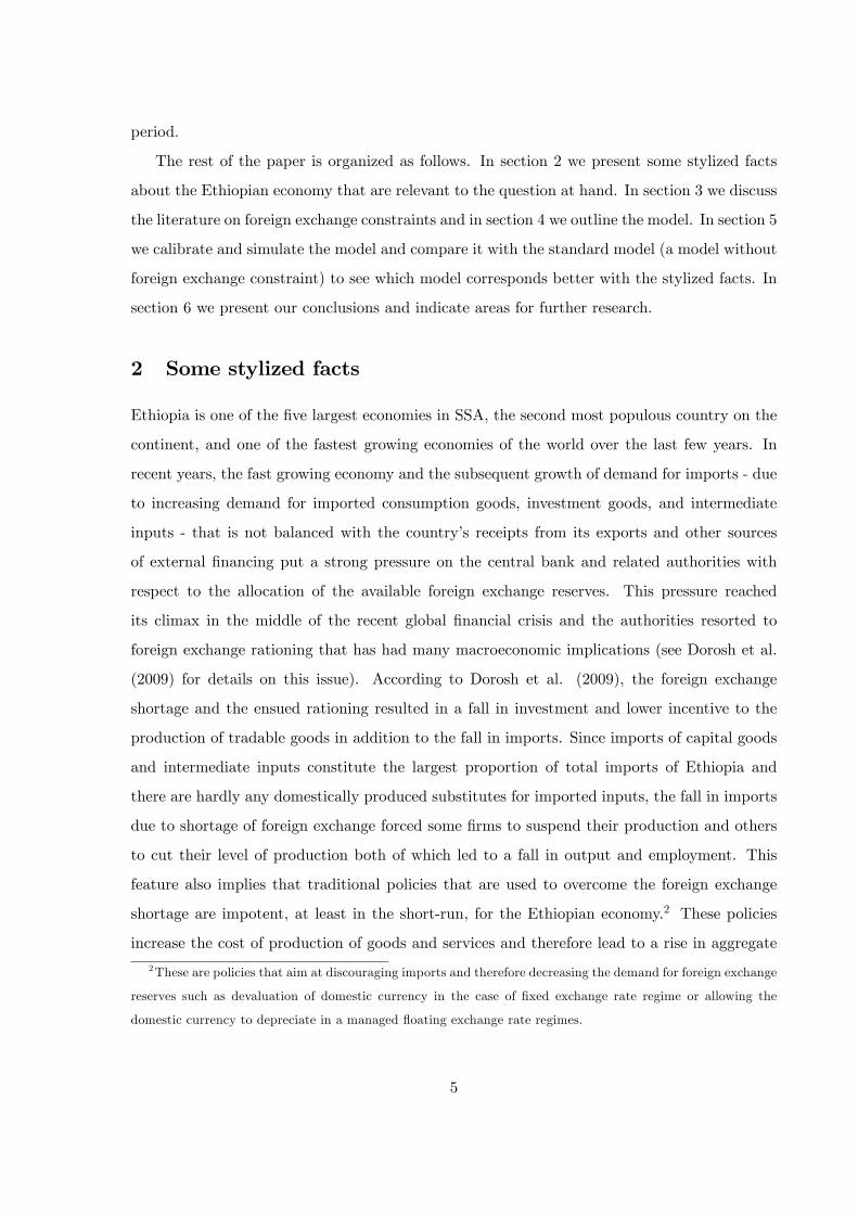
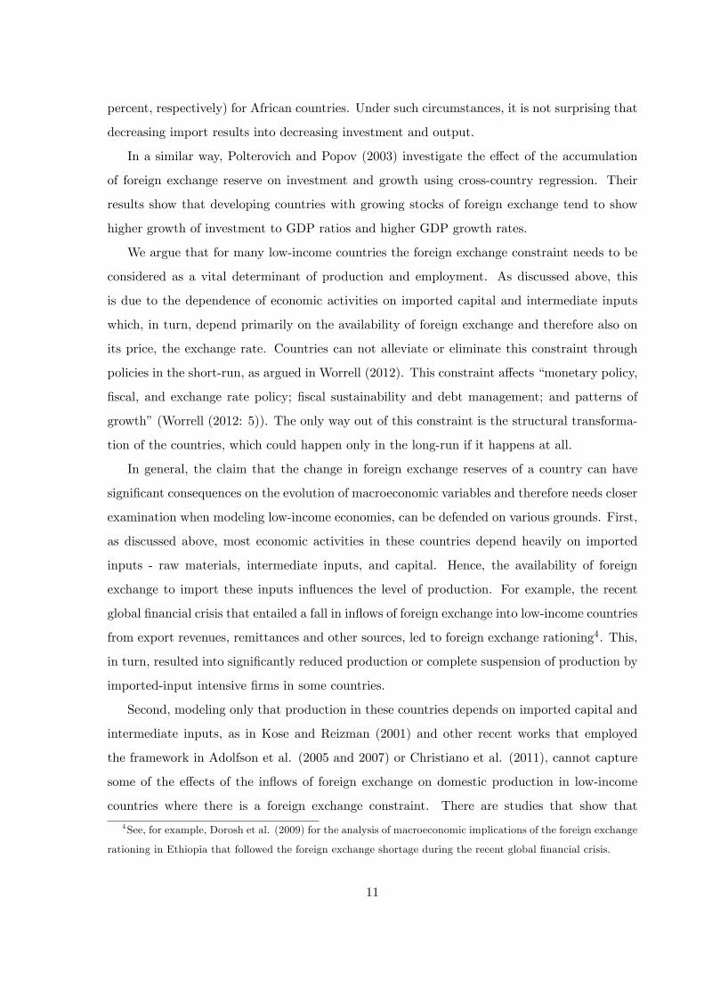
Figure 1: Export and import of goods and services

0 1965 1970 1975 1980 1985 1990 1995 2000 2005 20109.5

10

10.5

11

11.5

12Sub­Saharan Africa

Years

log

 (Exp

orts

) a

nd

 log

 (im

port

s)

importsexports

0 1985 1990 1995 2000 2005 20108.5

9

9.5

10Ethiopia

Years

log

(Exp

ort

s) a

nd

 log

(im

port

s)

importsexports

0 1985 1990 1995 2000 2005 20108.8

9

9.2

9.4

9.6

9.8

10Ethiopia

Years

log

 (Im

po

rts) 

an

d lo

g(X

+A+

Re

m)

importsX+A+Rem

Source: World Bank, WDI-GDF database, own calculation

First, the external sector of the Ethiopian economy has been characterized by signi�cant

imbalances for decades. For example, over the period 1981-2011, a period for which complete

data on the basic components of the national income accounts are available, the value of exports

of goods and services has always been signi�cantly lower than the value of imports of goods and

services. On average, the export earnings over the period amounted only to about 50 percent

of the import bills. For the SSA as a region the ratio of imports of goods and services to the

export of goods and services for the period 1981-2011 is almost 1. For Ethiopia this ratio comes

closer to 1 (0.95) only when one takes the ratio of imports of goods and services to the sum

of exports (X), net o¢ cial development assistance and o¢ cial aid received (A), and personal

remittances (Rem) as indicated in the lower panel of Figure 1.

6

Second, though there are no disaggregated long time series data on the composition of

imports, the largest proportion of imports seems to be intermediate inputs and capital goods.

According to Kose (2002) imports of capital goods and intermediate inputs represent about

75 percent of the total imports of goods (merchandise imports) for developing countries. For

Ethiopia, for the years 1995, 2005, and 2011 the proportions of imports of capital goods and

intermediate inputs in the total merchandise imports were 83.5, 87.2, and 85 percents, respec-

tively (UN (2012)).3 On the other hand, similar to the SSA region, imports of food constitute

only 11 percent of total imports of goods and services over the period 1993-2011, the period

for which data on this variable is available.

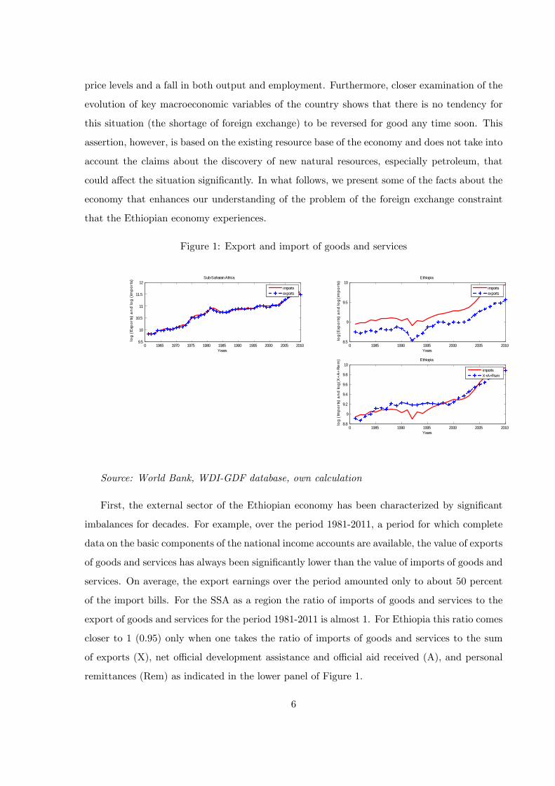
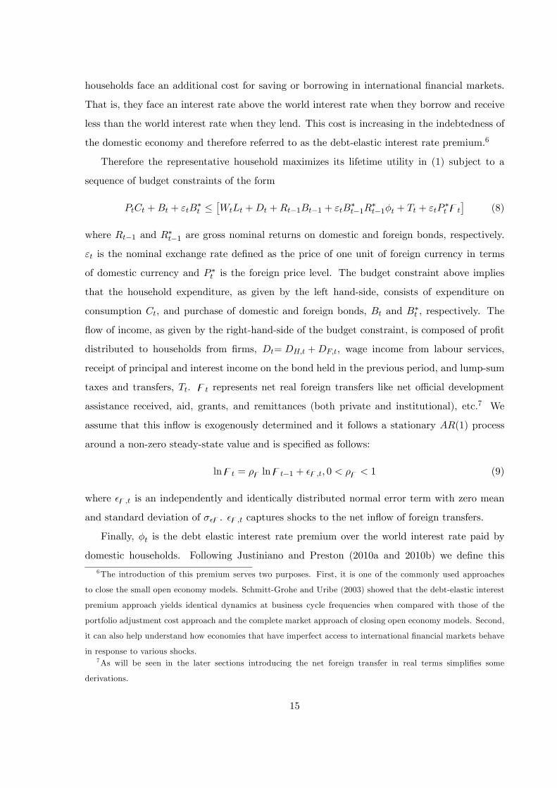
Figure 2: Growth rates of foreign exchange reserves, GDP, and imports of Ethiopia 1982-2009

1982 1986 1990 1994 1998 2002 2006 2010­1

0

1

2

3

4Growth of Reserves

Years

Per

cent

s

1982 1986 1990 1994 1998 2002 2006 2010­15

­10

­5

0

5

10

15Growth of GDP

Years

Per

cent

s

1982 1986 1990 1994 1998 2002 2006 2010­20

­10

0

10

20

30

40Growth of Imports

Years

Per

cent

s

Source: World Bank, WDI-GDF database

Third, close examination of the movements of some of the key macroeconomic variables of

the Ethiopian economy also shows some interesting insights. The growth rate of the foreign

exchange reserves moves in opposite direction relative to the growth rates of GDP and imports,

as shown in Figure 2. The correlation coe¢ cient between the growth rate of foreign exchange

reserves and GDP, both measured as annual percentage changes, is -0.45 while that between the

growth rates of foreign exchange reserves and imports is -0.2. The negative correlation between

3Following Kose (2002) we de�ned the imports of capital goods as imports of machinery and equipment

while imported intermediate inputs constitute imports of fuel plus all manufactured items minus machinery and

equipment.

7

the growth rate of foreign exchange reserves and growth rates of GDP and imports seems

to imply that periods of high economic growth are periods over which the foreign exchange

reserves run down due to high imports. The other feature of the macroeconomic variables of

the Ethiopian economy is that for almost all the variables we considered the variation of the

variables for Ethiopia are more than those of the regional averages as can be seen from Table

1. For example, the variability of the growth of GDP and the growth of imports of goods and

services are signi�cantly higher for Ethiopia than those of SSA region. Over the period 1981-

2011, Ethiopia had an average GDP growth rate of about 5 percent with a standard deviation

of 7 percent while the �gures for SSA are about 3 and 2 percents, respectively.

Table 1: Summary statistics for some relevant variables

SSA Ethiopia

Growth rates Mean Std Mean Std

GDP (a) 3.0624 1.9662 4.7900 6.9145

imports (b) 4.1319 6.1180 7.4105 11.0827

exports 3.5321 3.7314 6.2158 14.3759

Net ODA and Aid 1.7334 4.3962 2.7175 9.7533

reserves (c) 2.9450 27.1308

corr(a,c) -0.45

corr(b,c) -0.2

Source: World Bank, WDI-GDF database, own calculation

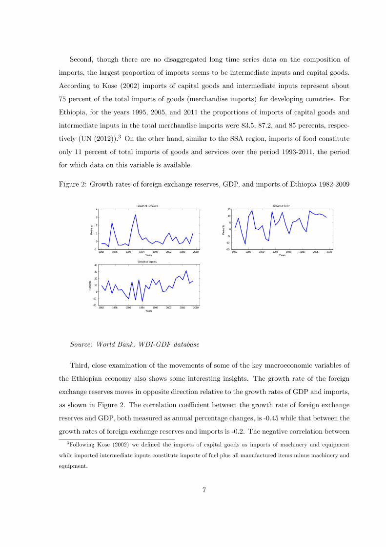
One of the measures of the health of the external sector of an economy is the foreign

exchange reserves that the economy has in its possession measured in terms of import cover

for certain months. The threshold varies from country to country depending on how much the

economy is vulnerable to exogenous shocks and the access it has to the international �nancial

markets. The IMF sta¤ report (IMF (2012)) on Ethiopia indicates that the country needs

to have foreign exchange reserves that can cover its import for at least 7.1 months. It is also

indicated in the same document that at the time of the preparation of the report (June - August

2012), Ethiopia�s import capacity was projected to be 1.8 months. The data over 1999-2009

show that the capacity of import cover of the economy on average was 3.3 months which was

decreasing over the last �ve years of the period (i.e., 2005-2009) to 2.6 months reaching its all

time low of 1.3 months in 2008.

8

Figure 3: The foreign exchange reserves in terms of the number of months of imports cover

1999 2000 2001 2002 2003 2004 2005 2006 2007 2008 20091

2

3

4

5

6

7

8

Mon

ths

Foreign exchange reserves in months of imports cover

actualrecommended (2012)

Source: World Bank, Global Economic Monitor, GEM data

Figure 3 shows the gap between the recommended foreign exchange reserves and what was

actually held over the period 1999-2009, assuming that the 7.1 months of imports was also the

appropriate threshold level during that speci�c period.

The absolute value of the quantity of the foreign exchange reserve for the threshold number

of months depends on the quantity and average prices of imports. The latter is exogenous

for economies like Ethiopia whereas the former changes only if preferences of households and

import content of domestic production change. However, both of these factors are not expected

to change in the short-run. Therefore, in the short-run, the central bank continues to grapple

with the problem of striking the right balance between satisfying the ever increasing demand for

foreign exchange due to an increasing demand for imports and maintaining some threshold level

of foreign exchange reserves to enhance the con�dence of both domestic and external economic

agents. This problem has also important implications on the availability and potency of policy

instruments that the central bank can employ to achieve the goals of stabilizing the economy in

the short-run and promoting growth in the long-run. The facts highlighted above are reasons

why we believe that Ethiopia is one of the best cases to analyze the e¤ects of foreign exchange

constraints and the shocks that a¤ect the in�ow of foreign exchange on the macroeconomic

dynamics of a country.

9

3 Foreign exchange constraints and developing countries

There are di¤erent studies, though not within the DSGE framework, that document the impor-

tant role that the availability and cost of foreign exchange play in the macroeconomic perfor-

mance of emerging and low-income countries (see, among others, Chenery and Bruno (1962),

McKinnon (1964), Porter and Ranney (1982), Marquez (1985), Khan and Knight (1988), Moran

(1989), Lensink (1995), Emran and Shilpi (1996), Polterovich and Popov (2003), Stiglitz et al.

(2006), and Agenor and Monteil (2008)). Porter and Ranney (1982), in a simple but very

instructive IS-LM framework, that is built based on a list of the characteristic features of the

macroeconomic environments of low-income economies, illustrate how the foreign exchange

constraint a¤ects the results of standard policy instruments. They argue that in a typical low-

income country, in the short run, expanding output without increasing cost of production could

be possible �provided only that foreign exchange can be located to purchase the needed raw

material imports� (p. 753). Agenor and Monteil (2008) and Stiglitz et al. (2006) also assert

that the availability of foreign exchange is a critical supply determining factor in developing

countries.

The empirical literature on this issue, though very limited, also supports this argument.

For instance, Moran (1989) studied the e¤ect of the fall in in�ow of foreign exchange in the

early 1980s due to declined foreign lending, rise in interest rates on debts, and fall in com-

modity prices, on volume and composition of imports of developing countries. His result shows

that most of the countries considered were a¤ected negatively. SSA countries, according to

Moran (1989), experienced a signi�cant fall in imports which, in turn, led to a deterioration of

investment and a fall or stagnant per capita output. Lensink (1995) also assessed the e¤ect of

the same phenomenon (fall in the foreign exchange in�ows into low-income countries in 1980s).

But unlike Moran (1989), Lensink (1995) investigated the e¤ect on overall macroeconomic

performance with an emphasis on economic growth. His simulation analysis shows that SSA

countries are among the hard-hit. He deduced that, other things being the same, improvement

of economic growth in low-income countries depends on the availability of foreign exchange

to import intermediate inputs. The results of these two studies imply that the imports of

low-income countries are mainly intermediate inputs and capital. This concurs with Kose and

Reizman (2001) that report that over the period 1970-1990 the proportion of intermediate

inputs and capital in the total imports was more than 75 percent (approximately 48 and 28

10

percent, respectively) for African countries. Under such circumstances, it is not surprising that

decreasing import results into decreasing investment and output.

In a similar way, Polterovich and Popov (2003) investigate the e¤ect of the accumulation

of foreign exchange reserve on investment and growth using cross-country regression. Their

results show that developing countries with growing stocks of foreign exchange tend to show

higher growth of investment to GDP ratios and higher GDP growth rates.

We argue that for many low-income countries the foreign exchange constraint needs to be

considered as a vital determinant of production and employment. As discussed above, this

is due to the dependence of economic activities on imported capital and intermediate inputs

which, in turn, depend primarily on the availability of foreign exchange and therefore also on

its price, the exchange rate. Countries can not alleviate or eliminate this constraint through

policies in the short-run, as argued in Worrell (2012). This constraint a¤ects �monetary policy,

�scal, and exchange rate policy; �scal sustainability and debt management; and patterns of

growth�(Worrell (2012: 5)). The only way out of this constraint is the structural transforma-

tion of the countries, which could happen only in the long-run if it happens at all.

In general, the claim that the change in foreign exchange reserves of a country can have

signi�cant consequences on the evolution of macroeconomic variables and therefore needs closer

examination when modeling low-income economies, can be defended on various grounds. First,

as discussed above, most economic activities in these countries depend heavily on imported

inputs - raw materials, intermediate inputs, and capital. Hence, the availability of foreign

exchange to import these inputs in�uences the level of production. For example, the recent

global �nancial crisis that entailed a fall in in�ows of foreign exchange into low-income countries

from export revenues, remittances and other sources, led to foreign exchange rationing4. This,

in turn, resulted into signi�cantly reduced production or complete suspension of production by

imported-input intensive �rms in some countries.

Second, modeling only that production in these countries depends on imported capital and

intermediate inputs, as in Kose and Reizman (2001) and other recent works that employed

the framework in Adolfson et al. (2005 and 2007) or Christiano et al. (2011), cannot capture

some of the e¤ects of the in�ows of foreign exchange on domestic production in low-income

countries where there is a foreign exchange constraint. There are studies that show that

4See, for example, Dorosh et al. (2009) for the analysis of macroeconomic implications of the foreign exchange

rationing in Ethiopia that followed the foreign exchange shortage during the recent global �nancial crisis.

11

increasing availability of foreign exchange in developing countries enhances the con�dence of

foreign investors (see, for instance, Polterovich and Popov (2003)). The argument is that an

increasing availability of foreign exchange in a country improves the ability of the country to

allow foreign investors to repatriate their pro�ts. This implies that the availability of foreign

exchange has also an external e¤ect since it attracts more �rms in addition to serving as an

input for already existing �rms. In other words, just like the relative resource abundance

attracts investors, at least in this part of the world, the availability of foreign exchange also

does.

Third, modeling the importance of the availability of foreign exchange can serve as a proxy

to capture the e¤ects of external �nancing (such as aid, loan, and remittance) on the perfor-

mance of the economy. Because in countries that face a foreign exchange constraint, in�ows

from these sources of external �nancing play a role beyond �lling the national resource gap;

that is they play a role that cannot be substituted by domestic savings (see McKinnon (1964)

and works cited there).

Fourth, according to Wyplosz (2007), some countries see accumulation of foreign exchange

reserves as an insurance against �nancial shocks which has signi�cant implications on macro-

economic performance. The argument is that accumulation of foreign exchange enhances the

con�dence of both domestic and foreign economic agents. For domestic producers and con-

sumers it implies that the country can a¤ord to continue imports while for foreign agents

dealing with the economy it gives the signal that the country can always meet its obligations,

even in the event of temporary shocks to the in�ow of foreign exchange.

Finally, modeling foreign exchange availability and its cost can also capture the e¤ect

of credit constraints faced by �rms in developing countries. Literature shows that one of

the constraints of �rms in developing countries is the lack of credit either as initial capital

(for investment � import of capital) or as working capital to import intermediate inputs or

both.5 This implies that the largest proportion of �rms�demand for credit is directly linked to

the foreign exchange constraint since most of both capital goods and intermediate inputs are

imported.

5Fafchamps (2004) in an extensive study of market institutions in SSA documents how the underdeveloped

�nancial markets lead to lack of credit for starting investment or for working capital by entrepreneurs. Fafchamps

(2004) also shows that most �rms in SSA countries are small and fail to grow to medium and large scale mainly

due to a shortage of formal credit to expand investment.

12

It is also important to indicate that, as a stylized fact, the in�ow of foreign exchange

into these countries shows signi�cant variability due to the erratic nature of export earnings,

aid, loans, and remittances. Furthermore, studies show that these in�ows from some of these

sources coincide with the performance of the domestic economy, with the shortage coming

when the economy needs foreign exchange most (see Bulir and Hamann (2008 and 2003)).

Thus, incorporating the foreign exchange constraint when modeling the macrodynamics of low-

income countries seems the most appropriate way to investigate how the economy responds to

global �nancial and trade shocks.

4 The model

The model in this paper is an extension of a model in Justiniano and Preston (2010a and

2010b) which builds on the work of Gali and Monacelli (2005) that lays out the structure of

a basic small open economy New Keynesian DSGE model. Therefore, many of the derivations

are based on Justiniano and Preston (2010a and 2010b) and Bäurle and Menz (2008).

4.1 Households

The household part of the model is captured by a representative, in�nitely lived household

that maximizes intertemporal utility from consumption and leisure. The household�s objective

function may be expressed as

E0

1Xt=0

�tUt (1)

where E is the expectation operator and � is the subjective discount factor of the households.

We assume that the representative household has the following instantaneous utility function:

Ut =(Ct � hCt�1)1��

1� � � � (Lt)1+'

1 + '(2)

where Ct and Lt, respectively, represent household consumption and labour time supplied to

market activities. � is the inverse of the elasticity of intertemporal substitution in consumption,

h is the coe¢ cient of habit persistence, ' is the inverse of the elasticity of labour supply, and

� is the marginal disutility (utility cost) of participating in the labour market.

Consumption Ct is a composite good consisting of home produced and imported goods that

13

can be given by the following CES aggregator:

Ct =

"(1� 1)

1�1 C

(�1�1)�1

H;t + 1�11 C

(�1�1)�1

F;t

#�1=(�1�1)(3)

where CH;t and CF;t denote consumption of domestic and imported goods, respectively. The

parameter �1 measures the elasticity of intratemporal substitution of consumption between

domestic and imported goods. 1 measures the proportion of imported goods in total household

consumption. The representative household aims at maximizing the utility from consumption of

both domestic and imported goods by minimizing the expenditure on these two varieties while

maintaining a certain target level of consumption. Solving this problem of optimal allocation

of expenditure on domestic and imported goods yields the following demand functions for these

goods:

CH;t = (1� 1)�PH;tPt

���1Ct (4)

and

CF;t = 1

�PF;tPt

���1Ct (5)

where PH;t, PF;t, and Pt are the price indices of domestic goods, imported goods, and overall

consumer goods, respectively. Both CH;t and CF;t are themselves bundles of di¤erentiated

goods where each variety is produced by a monopolistically competitive �rm. The overall

consumer price index is given by

Pt =h(1� 1) (PH;t)1��1 + 1 (PF;t)1��1

i1=(1��1)(6)

Total consumption expenditure by households is given by the sum of the expenditures on

domestic and imported goods they consume

PtCt = PF;tCF;t + PH;tCH;t (7)

Since they own the �rms in the economy, households earn dividends and also earn wage income

from the supply of their labour services. In this model there is no investment and therefore

no rental income from capital services. Furthermore, there is no �nancial sector and therefore

no �nancial intermediation. It is assumed that households can save in both domestic and

foreign one period bonds though their access to the international �nancial markets is imperfect.

This imperfection is captured by employing the debt-elastic interest rate premium approach

discussed in Benigno (2001). According to Benigno (2001), this approach assumes that domestic

14

households face an additional cost for saving or borrowing in international �nancial markets.

That is, they face an interest rate above the world interest rate when they borrow and receive

less than the world interest rate when they lend. This cost is increasing in the indebtedness of

the domestic economy and therefore referred to as the debt-elastic interest rate premium.6

Therefore the representative household maximizes its lifetime utility in (1) subject to a

sequence of budget constraints of the form

PtCt +Bt + "tB�t �

�WtLt +Dt +Rt�1Bt�1 + "tB

�t�1R

�t�1�t + Tt + "tP

�t zt

�(8)

where Rt�1 and R�t�1 are gross nominal returns on domestic and foreign bonds, respectively.

"t is the nominal exchange rate de�ned as the price of one unit of foreign currency in terms

of domestic currency and P �t is the foreign price level. The budget constraint above implies

that the household expenditure, as given by the left hand-side, consists of expenditure on

consumption Ct, and purchase of domestic and foreign bonds, Bt and B�t , respectively. The

�ow of income, as given by the right-hand-side of the budget constraint, is composed of pro�t

distributed to households from �rms, Dt= DH;t +DF;t, wage income from labour services,

receipt of principal and interest income on the bond held in the previous period, and lump-sum

taxes and transfers, Tt. zt represents net real foreign transfers like net o¢ cial development

assistance received, aid, grants, and remittances (both private and institutional), etc.7 We

assume that this in�ow is exogenously determined and it follows a stationary AR(1) process

around a non-zero steady-state value and is speci�ed as follows:

lnzt = �z lnzt�1 + �z;t; 0 < �z < 1 (9)

where �z,t is an independently and identically distributed normal error term with zero mean

and standard deviation of ��z. �z,t captures shocks to the net in�ow of foreign transfers.

Finally, �t is the debt elastic interest rate premium over the world interest rate paid by

domestic households. Following Justiniano and Preston (2010a and 2010b) we de�ne this

6The introduction of this premium serves two purposes. First, it is one of the commonly used approaches

to close the small open economy models. Schmitt-Grohe and Uribe (2003) showed that the debt-elastic interest

premium approach yields identical dynamics at business cycle frequencies when compared with those of the

portfolio adjustment cost approach and the complete market approach of closing open economy models. Second,

it can also help understand how economies that have imperfect access to international �nancial markets behave

in response to various shocks.7As will be seen in the later sections introducing the net foreign transfer in real terms simpli�es some

derivations.

15

premium as

�t = exp [�� (at�1 +$t)]

at�1 �"t�1B�t�1Y FPt�1

which is the real quantity of outstanding foreign debt expressed in terms of domestic currency

as a fraction of steady-state import and $t is a risk premium shock.8 Justiniano and Pre-

ston (2010a and 2010b) assert that the above functional form for the risk premium ensures

stationarity of the foreign debt level in a log-linear approximation to the model.

The optimization problem faced by the representative household can now be summarized

by the following Lagrangian function:

MaxCt;Lt;Bt;B�t

1Xt=0

�t

8>>>><>>>>:(Ct � hCt�1)1��

1� � � � (Lt)1+'

1 + '

��t

24 PtCt +Bt + "tB�t �Dt �W tLt�Rt�1Bt�1

�"tB�t�1R�t�1�t � Tt + "tP �t zt

359>>>>=>>>>; (10)

The �rst order conditions of the optimization problem of this household are given by

(Ct � hCt�1)�� = �tPt (11)

� (Lt)' = �tWt (12)

�Et�t+1Rt = �t (13)

�Et�t+1"t+1R�t�t+1 = �t"t (14)

Conditions (11) and (12) can be combined to give the marginal rate of substitution between

consumption and labour

� (Lt)' (Ct � hCt�1)� =

Wt

Pt

while combining (11) and (13) gives the domestic households�Euler equation of consumption

�Et(Ct+1 � hCt)��

(Ct � hCt�1)��PtPt+1

=1

Rt

Similarly, the combination of (13) and (14) yields the UIP condition

�Et�t+1Rt = �Et�t+1"t+1"t

R�t�t+1

8This risk premium is exogenous to the households as it depends on aggregate variables and, therefore, in

making their decisions households take the risk premium as given.

16

4.2 Firms

Domestic goods are produced by a continuum of identical monopolistically competitive �rms

using capital, labour, and imported intermediate inputs. This is standard speci�cation in the

literature. The main di¤erence between the production functions in the literature and ours

is that we assume that the intermediate inputs used in the production of domestic goods are

imported by �rms that face foreign exchange constraints. Therefore, the availability of foreign

exchange a¤ects the level of domestic production since the price and quantity of imported

intermediate inputs depend on the availability of foreign exchange, which in turn depends on

the export earnings of the country and the country�s access to international �nancial markets.

There are also a continuum of monopolistically competitive �rms that import homogenous

goods and package (brand name) and supply these goods to the domestic retailers. As indicated

in the previous section, the quantity of goods imported by these �rms is determined by the

quantity of foreign exchange made available to them by the central bank.

4.2.1 Domestic production

Domestic producers employ labour L, capital K, and imported intermediate inputs M , to

produce goods that are either consumed domestically or exported to the rest of the world.

However, capital does not appear in our model for the sake of simplicity and following the

tradition in many works in the area.9 The production function is a simple Cobb-Douglas type

with constant returns to scale

YH;t= ZH;tL�1t M

�2t , (�1 � 0; �2 � 0, �1 + �2 = 1) (15)

where YH;t denotes the output level of domestic production and ZH;t is the total factor pro-

ductivity of the domestic economy. We assume that the total factor productivity follows a

stationary autoregressive process of order one, AR(1), in its logarithm as follows:

lnZH;t = �H lnZH;t�1 + �H;t, 0 < �H < 1. (16)

where �H,t is an independently and identically distributed normal error term with zero mean

and standard deviation of ��H .9See Walsh (2010, p. 330) on why capital is absent in the New Keynesian DSGE model.

17

The objective of a representative �rm in this sector can be given as minimizing the cost of

production given the production level

minLN;t;Mt

(WtLt + PFtMt) subject to YH;t = ZH;tL�1t M

�2t (17)

Solving this problem for LH;t and Mt we obtain the conditional demand functions for the two

inputs given by

Lt =

��1�2

��2P�2F;tW

��2t YH;tZ

�1H;t (18)

and

Mt =

��2�1

��1P��1F;t W

�1t YH;tZ

�1H;t (19)

We can substitute these demand functions into the objective function to obtain the total cost

function of the �rm in terms of input prices, share parameters, total productivity term, and

output level from which the real marginal cost function is derived as

MCH;t =

"��2�1

��1+

��2�1

���2# P�2F;tW�1t Z�1H;tPt

(20)

4.2.2 Price setting by domestic producers

Domestic producers face price setting frictions. They set their prices according to the Calvo

staggered price setting mechanism allowing for indexation to past price in�ation of domestically

produced goods as in Justiniano and Preston (2010a and 2010b). Accordingly, in any period

t a random fraction 1� &H of �rms can optimally reset their prices while the remaining &H of

�rms index their prices to recent past in�ation as in

PH;t (i) = PH;t�1 (i)

�PH;t�1PH;t�2

��H(21)

where �H measures the weight these backward-looking �rms attach to past in�ation. On the

other hand, the �rm that can reoptimize its price in period t chooses its optimal price, P0H;t,

that maximizes the present discounted value of pro�ts taking into account the probability that

it may not be able to re-set prices for some time in the future. Since home goods are consumed

by both domestic and foreign households the �rm�s demand is the sum of the two demands.

Assuming symmetric preferences between domestic and foreign households we have the same

functional form for the two demands. Therefore, the demand curve faced in period t+ � by a

�rm that last re-set its price optimally in period t and since then just adjust prices according

18

to the indexation rule above is given by

CH;t+� jt =

P0H;t

PH;t+�

�PH;t+��1PH;t�1

��H!��1 �CH;t+� + C

�H;t+�

�(22)

The expected discounted pro�t for this �rm is given by

1X�=0

&�H�t;t+�CH;t+� jt

"P0H;t

�PH;t+��1PH;t�1

��H� PH;t+�MCH;t+�

#where �t;t+� is the stochastic discount factor and MCH;t+� is the real marginal cost of the

home goods producing �rms. The �rst order necessary condition of the above problem gives

P0H;t =

�2�2 � 1

P1�=0 &

�HEt

��t;t+�CH;t+� jtPH;t+�MCH;t+�

�P1�=0 &

�HEt

h�t;t+�CH;t+� jt (PH;t+��1=PH;t�1)

�Hi (23)

Since all �rms that can reset their prices face the same decision problem they set the same

price denoted by P0H;t. Therefore, the aggregate price index of domestically produced tradable

goods is given by the CES function of the two types of prices

PH;t =

24(1� &H)P 01��1H;t � &H

PH;t�1 (i)

�PH;t�1PH;t�2

��H!1��135 11��1

(24)

As we show in the appendix, log-linear approximation of the combination of (23) and (24)

yields the hybrid New Keynesian Phillips Curve for the domestically produced goods.

4.2.3 Importing �rms and the foreign exchange constraint

As indicated in the introductory section, the novelty of this study is the introduction of the

foreign exchange constraints that the economy faces to satisfy its demand for imports into an

otherwise standard small open economy New Keynesian model. The basic approach we follow

to model the import sector is the one developed in Christiano et al. (2011) with the main

di¤erences being the types of importing �rms and the foreign exchange constraints. Unlike

Christiano et al. (2011) who model three types of importing �rms (consumption goods, invest-

ment goods, and intermediate inputs) we have only one type of importing �rms that import

foreign goods used in the domestic economy as both consumption goods, CF;t, and intermedi-

ate inputs, Mt. Furthermore, in our model importing �rms face a foreign exchange constraint.

There are continuum of identical monopolistically competitive �rms of measure 1 that import

these goods. These �rms import homogenous goods and package (brand name) the homoge-

nous goods into di¤erentiated (specialized) �nal goods and sell them to domestic retailers who

19

are perfectly competitive. The importing �rms pay for their imports in foreign currency but

sell their goods to the domestic retailers in domestic currency. Therefore they need to locate

foreign currency at the beginning of the period. This characterization of the import sector is

identical to the one in Christiano et al. (2011). Our departure from their approach is that

the importing �rms in their model can borrow as much foreign currency as they want at the

on going foreign interest rate while those in our model cannot. For simplicity, we assume that

importers have the necessary amount in terms of domestic currency and their problem is ob-

taining the foreign currency equivalent.10 In the real world, this demand for foreign currency

is satis�ed by commercial banks that buy foreign currency from the central bank and sell or

lend it to importers. Since there are no commercial banks in our model, we assume that the

importing �rms buy the foreign exchange directly from the central bank.

The basic assumption underlying this study is that there is a gap between the quantity of

foreign exchange demanded by importing �rms (derived from households�and �rms�demand

for imports) and the quantity of foreign exchange that the central bank can make available.

One way to think about this problem is that at the beginning of every period t importing

�rms submit their request for foreign exchange to the central bank. The quantity of foreign

exchange requested by importing �rms, in turn, is derived from the quantities of imports de-

manded by households and �rms. Suppose the aggregate quantity of imported consumption

goods and intermediate inputs demanded at the price level without the foreign exchange con-

straints are given by (YF;t)u = (CF;t)

u + (Mt)u, where u denotes unconstrained quantity. The

existence of a foreign exchange constraint implies that the central bank can satisfy only a

certain fraction �F;t of the quantity demanded of the foreign exchange (or the quantity de-

manded of imports). Suppose we denote the actual (or the constrained) quantities of imports

by YF;t = CF;t +Mt. It follows that

YF;t = �F;t (YF;t)u , 0 < �F;t � 1 (25)

10Note that one can drop this assumption and in stead assume that importing �rms borrow the foreign

exchange they need at the beginning of the period as in Christiano et al. (2011). But the �rms still face the

constraint since the foreign exchange available for imports is less than the quantity demanded and as a result

the authorities resort to rationing what is available based on certain criteria. This assumption adds one more

dimension to the problem: the marginal cost of the importing �rms becomes a function of foreign interest rate

in addition to the exchange rate, the foreign currency price of imports, and the shadow price of the availability

of foreign exchange.

20

In other words, the central bank issues import licenses that are certain proportions of what

is demanded by importing �rms. There are many factors that the central bank takes into

consideration in determining YF;t the discussion of which we defer to a later section where we

discuss the central bank�s problem of foreign exchange reserves management.

In what follows we discuss how this problem translates into the decision making process of

individual importing �rms. Assume that at the beginning of every period t the central bank

rations a certain quantity of foreign exchange P �t YF;t. As indicated above, both types of goods

are imported by a continuum of identical monopolistically competitive �rms of measure 1 to

which the central bank rations the available foreign exchange. For the sake of simpli�cation, we

assume that the available foreign exchange is distributed equally; i.e., each importing �rm i faces

the same foreign exchange constraint P �t YiF;t. We assume that this constraint is always binding

except at the steady-state. At the aggregate level P �t YF;t =R 10 P

�t YiF;tdi. As we highlighted

in the preceding paragraph, the central bank can supply only a given fraction of the quantity

of foreign exchange demanded. Accordingly, we assume that a speci�c importing �rm submits

a request to import (YF;t (i))u but it is given foreign exchange that is a certain fraction �F;t

of the requested amount where 0 < �F;t � 1. That is, the foreign exchange distributed (or,

in other words, the importing license issued) to each �rm is YF;t (i) = �F;t (YF;t (i))u. Since,

by assumption, the constraint is not binding at the steady state the two quantities are equal -

that is, �F;t = 1.

It simpli�es the discussions and the derivations below to assume that there are perfectly

competitive �rms between the importing monopolistically competitive �rms and the end users

of imports - households and domestic goods producing �rms.11 These �rms package the di¤er-

entiated consumption goods and intermediate inputs and sell them to households and �rms and

are price takers at both the input and output markets. For an individual perfectly competitive

�rm that packages YF;t we have the following production function

YF;t =

�Z 1

0(YF;t (i))

�F�1�F di

� �F�F�1

The pro�t maximization problem of this perfectly competitive �rm is given by

PF;t

�Z 1

0(YF;t (i))

�F�1�F di

� �F�F�1

�Z 1

0PF;t (i)YF;t (i)

11This assumption is similar to the assumption in Christiano et al. (2011).

21

Solving this pro�t maximization problem we obtain its demand function for each specialized

input

YF;t (i) =

�PF;t (i)

PF;t

���FYF;t (26)

Equation (26) is the demand function of a perfectly competitive retailer for a speci�c variety

of imported goods, YF;t (i). In other words, it is the demand function faced by the �rm that

imports YF;t (i).

Now let�s discuss the optimization problems of the importing �rms. To see the e¤ect of the

foreign exchange constraint on optimal price of the �rm and the quantity imported we derive

and compare the outcomes under the two conditions. We �rst outline the optimal price of a

speci�c importing �rm without the constraint. The speci�c importing �rm takes the price of

its imports and the demand for its speci�c import, YF;t (i), given above to maximize its pro�t.

That is, the �rm solves the following maximization problem

maxPF;t(i)

(PF;t (i)� "tP �t )YF;t (i)

subject to (26). Solving the problem we have the optimal price that the �rm would like to

charge for its imports if there are no price setting frictions - the usual mark-up price

(PF;t (i))u =

�F(�F � 1)

"tP�t (27)

where the superscript u denotes the unconstrained condition.

Now assume that the importing �rms face the foreign exchange constraints and therefore

the quantity of their imports is always smaller than the level that they would like to import

without the constraint (the output level dictated by the demand for imported goods from the

households and �rms at the price level (27)). The objective of the speci�c importing �rm is to

maximize pro�t given the foreign price of its imports, the demand function it faces, and the

foreign exchange constraint. The problem of the �rm can be summarized as

maxPF;t(i)

(PF;t (i)� "tP �t )YF;t (i)

subject to (26) and

YF;t (i) � �F;t (YF;t (i))u

The Lagrangian of this speci�c �rm is given by

L = (PF;t (i)� "tP �t )�

PF;tPF;t (i)

��FYF;t � �F;t

""tP

�t

�PF;tPF;t (i)

��FYF;t � "tP �t �F;t (YF;t (i))

u

#

22

Solving the above problem of the importing �rm gives the optimal price that the �rm would

like to charge

PF;t (i) =�F

(�F � 1)"tP

�t

�1 + �F;t

�(28)

This is the optimal price that the importing �rm charges absent any price setting friction -

again the usual mark-up over its marginal cost except this time there is an additional term to

the �rm�s marginal cost - the Lagrangian multiplier to the foreign exchange constraint.

The Lagrangian multiplier �Ft in (28) measures the change in the optimal price that im-

porters would like to charge as a result of the change in the quantity of foreign exchange that the

central bank makes available for imports.12 Comparing (27) and (28) we can see that as long

as the constraint is binding, �F;t > 0, the price of imported goods under the foreign exchange

constraints is always greater than the price without the constraints. Furthermore, as usual

the value of �F;t depends on the tightness of the constraint - in this case the foreign exchange

constraint. That is, �F;t is some positive function of the di¤erence between the foreign exchange

requested and the quantity distributed by the central bank; when the constraint is not binding

the gap between the two is zero and �F;t is also zero. This tightness of the foreign exchange

constraint can be captured by the gap between the constrained and the unconstrained quantity

of imports. What are then the speci�c relationships between �F;t and (YF;t (i))u � YF;t (i)?

Since the introduction of a foreign exchange constraint is observed by the end users of

imports - households and �rms - in terms of changes in prices, the demand function of the

households and �rms for imported goods remain the same with and without the foreign ex-

change constraint. This implies that an importing �rm faces the same demand function for its

speci�c imports whether it faces the constraint or not. This, in turn, implies that YF;t= (PF;t)��F

for YF;t (i) importing �rm remains the same with and without the foreign exchange constraint.

Therefore, using these facts and the demand function faced by an individual importing �rm

(26) we can derive the speci�c relationship between the Lagrangian multiplier, �F;t, and the

ratio of the unconstrained imports, (YF;t)u, to constrained imports, YF;t, as

�F;t =

�1

�F;t

� 1�F � 1 (29)

or

�F;t =

�(YF;t)

u

YF;t

� 1�F � 1 (30)

12This multiplier can loosely be interpreted as a rent created due to the foreign exchange rationing.

23

The above relationship shows that as long as the ratio between the imports under the two

conditions is di¤erent from 1 (�F;t < 1), the constraint is binding and therefore the value of

the Lagrangian multiplier is greater than zero - implying that the optimal price charged by

the importing �rms is always greater than the optimal price without the constraint. At the

stedy-state when the foreign exchange constraint is assumed to be not binding (�F;t = 1),

�F;t = 0. This implies that the quantity restriction that is imposed by the foreign exchange

constraint allows the importing �rms to charge higher prices compared to their optimal prices

that they would like to charge without the constraint. This is consistent with both intuition

and economic theory. Furthermore, the di¤erence between the constrained and unconstrained

prices is increasing as the gap between the constrained and unconstrained imports increases

(that is, as �F;t decreases) while it decreases with increasing degree of substitutability between

the varieties imported. That is, all other things remaining the same, the higher the elasticity

of substitution between the varieties of the imported goods, the lower the value of Lagrangian

multiplier and vice versa.

The decisions of the central bank on the quantity of foreign exchange distributed to im-

porters and the desired quantity of imports by households and �rms determine the values of

�F;t which, in turn, determines the values of �F;t.13

4.2.4 Price setting by importing �rms

As indicated above, absent any price setting friction, the optimal price that importing �rms

would like to charge is PF;t (i) = (�F = (�F � 1))"tP �t�1 + �F;t

�. However, as with the domestic

goods producers, importing �rms face price setting frictions. Assume that in any period t a

random fraction 1� &F of �rms can optimally reset their prices while the remaining &F of �rms

index their prices to recent past in�ation as in

PF;t (i) = PF;t�1 (i)

�PF;t�1PF;t�2

��F(31)

13Note that our modeling assumes that the central bank does not have a bias between imports of consumption

goods and intermediate inputs. However, one can model the importers of consumption goods and intermediate

inputs separately and experiment on the e¤ects of the changes on the distribution of the available foreign exchange

reserves to the two types of imports on some key macroeconomic variables like output level, employment, and

in�ation rate. Our model assumes that the central bank distributes the same proportions of the requested foreign

exchange reserves for both types of �rms; that is, �ct = �mt = �Ft where c and m stand for the consumption

and intermediate inputs, respectively.

24

where �F measures the weight that these backward-looking �rms attach to past in�ation. On

the other hand, a �rm that resets its optimal price in period t maximizes the present discounted

value of pro�ts by choosing its optimal price P0F;t, taking into account the probability of not

being able to re-set prices in the future. The demand curve faced in period t + � for a �rm

that last re-set prices optimally in period t and henceforth just adjust prices according to the

indexation rule is given by

YF;t+� jt =

P0F;t

PF;t+�

�PF;t+��1PF;t�1

��F!��FYF;t+� (32)

The expected discounted pro�t for this �rm is given by

1X�=0

&�F�t;t+�YF;t+� jt

"P0F;t

�PF;t+��1PF;t�1

��F� PF;t+�MCF;t+�

#where �t;t+� is the stochastic discount factor and MCF;t+� is the real marginal cost of the

consumption goods importing �rms. The �rst order necessary condition of the above problem

gives

P0F;t =

�F�F � 1

P1�=0 &

�FEt

��t;t+�YF;t+� jtPF;t+�MCF;t+�

�P1�=0 &

�FEt

h�t;t+�YF;t+� jt (PF;t+��1=PF;t�1)

�Fi (33)

Since all �rms that can reset their prices face the same decision problem they set the same

price denoted by P0F;t. Therefore, the aggregate price index of imported consumption goods is

given by the CES function of the two types of prices

PF;t =

24(1� &F )P 01��FF;t � &F

PF;t�1 (i)

�PF;t�1PF;t�2

��F!1��F35 11��F

(34)

The log-linear approximation of the combination of (33) and (34) yields the hybrid New Key-

nesian Phillips Curve for the imported goods.

4.3 Market clearing conditions

Goods market clearing in the domestic economy requires that domestic output is equal to

the sum of domestic consumption and foreign consumption of domestically produced goods or

exports. This implies

Yt = YH;t = CH;t + C�H;t (35)

We know that

CH;t = (1� 1)�PH;tPt

���1Ct

25

then foreign consumption of domestically produced tradable goods (exports) must be

C�H;t = 1

�PH;t"tP �t

���1C�t (36)

The domestic currency denominated bond is held only by domestic economic agents. There-

fore, at the aggregate level the net supply of this bond is zero. Furthermore, assuming that

all households in the economy face the same budget constraint and aggregating for the whole

economy we have the net foreign asset position of the economy given by14

"tB�t = "tB

�t�1R

�t�1�t + "tP

�t zt + PH;tC�H;t � "tP �t YF;t (37)

4.4 The monetary policy rule

Many works indicate that low-income countries like Ethiopia employ monetary policy regimes

that are quite di¤erent from the simple or modi�ed Taylor rule common in the DSGE litera-

ture.15 However, our objective in this paper is to examine how the introduction of the foreign

exchange constraints a¤ects the behaviour of key macroeconomic variables given the other parts

of the standard model are maintained. Hence, we defer the modi�cation of monetary policy

rules to subsequent work and in this study we use the simple Taylor type rule where the mon-

etary authority is assumed to act to stabilize in�ation, output and exchange rate. According

to this rule, the monetary authority adjusts the nominal interest rate in response to deviations

of in�ation, output, and exchange rate from their steady-state or target values

Rt

R=

�Rt�1

R

��r "� PtPt�1

��� �YtY

��y � "t"t�1

���e#(1��r)�r;t (38)

where ��, �y, and �e are weights put by monetary authority, respectively, on in�ation, GDP,

and depreciation of the exchange rate. The lagged interest rate serves for interest rate smooth-

ing while �r denotes the extent of persistence of interest rate. The monetary policy shock is

captured by �r;t.

4.5 Foreign Exchange accumulation

As discussed in the previous section, the central bank also decides on the quantity of foreign

exchange it makes available for imports. This decision can also be seen as an important pol-14For the details see the appendix.15For details, see Adam et al. (2009, 2008). Also see Mishra and Montiel (2012) and Mishra et al. (2012) for

discussion on the weakness and/or absence of the conventional monetary transmission mechanism in low income

countries.

26

icy instrument for monetary authorities in countries that face foreign exchange constraint and

where almost all other components of their balance of payments are exogenously determined

(see Hemphill (1974)). This argument stems from the fact that for countries like Ethiopia the

e¤ect of domestic policies on their export revenues, remittances, foreign aid and assistance,

foreign investment, and access to foreign loan is very weak if any. But by changing the quan-

tity of foreign exchange available to imports the central bank can in�uence imports almost

immediately and thereby the external balance of the economy. The foreign exchange in�ow at

any period is given by the usual balance of payments identity as

t = t�1 +B�t +B

�t�1R

�t�1�t + P

�t zt + P �t C�H;t � P �t YF;t (39)

where t is end of period foreign exchange reserves of the central bank and the other variables

are as de�ned in the previous sections.

The central bank takes many factors into account in its decision on how much of the

available foreign exchange to distribute to importers and how much of it to hold as reserves.

For simpli�cation, we assume that there are three main factors that the bank considers. First,

the central bank is assumed to have a certain target (operational) level of foreign exchange

reserves as discussed in section 2. Therefore, it tries to minimize the deviation of the end-

of-period foreign exchange reserves from this target level. Large deviations are not consistent

with the objectives of the bank, since a large positive deviation implies ine¢ cient resource

utilization while a large negative deviation implies exposure of the economy to high risks of

external shocks. Second, the central bank tries to smooth imports by reducing the deviations of

current imports from that of the previous period. Third, the central bank aims at minimizing

the di¤erence between the quantity of imports demanded (or the desired import level) and the

actual quantity imported since this gap has rami�cations on other macroeconomic variables. In

our analysis, this gap is measured as the di¤erence between the quantity of imports demanded

by households and �rms at the price level without the foreign exchange constraint and the

actual quantity of imports (the foreign exchange that the central bank can make available

divided by the foreign price level). It is reasonable to assume that the central bank takes the

desired level of imports into consideration when it makes decision on the quantity of foreign

exchange that it distributes to the importing �rms since the larger the gap between the two

quantities, the larger will be the pressure on the in�ation of imported goods. This, in turn,

puts pressure on aggregate in�ation depending on the share of imported goods prices in the

27

aggregate price level. Since stabilizing prices is one of the goals of the central bank, it tries

to reduce this pressure on aggregate in�ation by reducing the gap between the two quantities.

Therefore, other things remaining the same, the central bank attempts to eliminate this gap.

Since the simultaneous achievement of the above goals is impossible the central bank faces

trade-o¤s that can be summarized by some form of loss function that it minimizes. We assume

that the central bank has some quadratic loss function which it minimizes by choosing optimal

values of end-of-period foreign exchange holdings t and imports YF;t. The functional form we

employed is inspired by the discussions in Hemphill (1974) and Moran (1989) and is given by

L =h��t �

�2+ �uP

�t (YF;t � (YF;t)

u)2 + �YF;t�1P�t (YF;t � YF;t�1)

2i

(40)

The central bank minimizes the above loss function subject to the change in foreign exchange

in�ows given in (39). The �is are weights that the central bank attaches to the deviation of the

end-of-period foreign exchange reserves from the target level, the deviation of current imports

from the desired level of imports, and the deviation of current imports from previous period

imports. Solving the loss minimization problem of the central bank we obtain the optimal level

of end of period foreign exchange holdings and the quantity of imports given below.

YF;t =�

�!t�1 + b�t + b

�t�1R

�t�1�t +zt + C�H;t

�� �! + �u (YF;t)u + �YF;t�1YF;t�1�

�u + �YF;t�1 + �

� (41)

and

!t =

264 !t�1 + b�t + b�t�1R

�t�1�t +zt + C�H;t

��(b�t+b�t�1R�t�1�t+zt)��!+�u(YF;t)

u+�YF;t�1YF;t�1�

�u+�YF;t�1+�

�375 (42)

where !t, !t�1, b�t , b�t�1, and ! are, respectively, t, B

�t , B

�t�1, and de�ated by the foreign

price level P �t (see the appendix for details).

4.6 The external sector

The model economy is small relative to the global economy and therefore it cannot a¤ect the

foreign variables like income, in�ation, interest rate, etc. Hence, the foreign economy can be

modelled as exogenous. Following the literature, we assume that the foreign variables (foreign

income, interest rate, and in�ation) follow stationary �rst order autoregressive AR(1) processes

in their logarithm.

28

5 Calibration and simulation

5.1 Calibration of parameters

To the best our knowledge this is the �rst New Keynesian model to be calibrated to the

Ethiopian economy. One of the problems with the calibration or estimation of macroeconomic

models for low-income countries like Ethiopia is the availability of appropriate data. The data

on some macroeconomic variables that are important for our study are either short time series

or not available at all. Furthermore, there are few works on macroeconomic dynamics of the

country and few microeconomic studies of macroeconomic relevance from which we can borrow

some of the parameters for our calibration. These make the calibration process somewhat

di¢ cult and, therefore, the resulting work is at best suggestive. We relied on the national

income accounts data of the country as much as possible to tie down the steady-state ratios

and estimate some of the parameters. The primary data used comes from the World Bank WDI-

GDF dataset and covers the period 1981-2012, and from the annual reports of the National Bank

of Ethiopia for various years. These data are used to tie down the steady-state ratios as long-run

averages. For the exogenous processes for which there is long time series data such as the net

foreign transfers and the variables of the rest of the world we estimated the parameters. Some

of the parameters and steady-state ratios are �xed in order to ensure the internal consistency

of the model. For parameters for which we are unable to determine values either because there

are no relevant data to estimate or there are no previous macro or microeconometric works on

Ethiopia, we used the values reported in other macroeconomic studies conducted on other SSA

countries or other low-income countries. In what follows we discuss the calibration process and

the values chosen for the steady-state ratios and the parameters. We �rst discuss the steady-

state ratios and then we present the parameters of preferences, technology, policy, and the rest

of the world in line with the order of our presentation of the model in the preceding section.

The complete list of the steady-state ratios and the parameters together with their values are

given in Tables 2-5.

The steady-state ratio of the real net foreign transfers to imports, �z, is �xed at 0:5 which

is based on our discussion in section 2 where we indicated that the long-run average of the ratio

of these in�ows to import is about 50 percent. On the other hand, the steady-state proportion

of imported consumption goods, �F , is �xed at 0:3 using the national income accounts data

for the period 2000 - 2011 - the period for which disaggregated data on imports by end users

29

is available. The steady-state ratio of prices of domestically produced goods to the overall

consumer price index, �H , is determined as the ratio of the price index of exports to CPI

assuming, as is the case in the model, that the LOP holds for exports and therefore domestic

currency prices of domestically consumed and exported domestically produced goods are the

same. In determining the value of �!, the steady-state ratio of imports to the central bank�s

foreign exchange reserves, we assume that the central bank�s target level of foreign exchange

reserve is the 7:1months of import cover recommended by IMF (2012), as discussed in section 2.

This implies that at the steady-state the foreign exchange reserves of the central bank equals

this operational target which �xes �! at 1:69. The proportions of imported consumption

goods and domestically consumed home produced goods are calculated such that the share of

consumption in GDP and the share of imports in GDP are inline with the data in the national

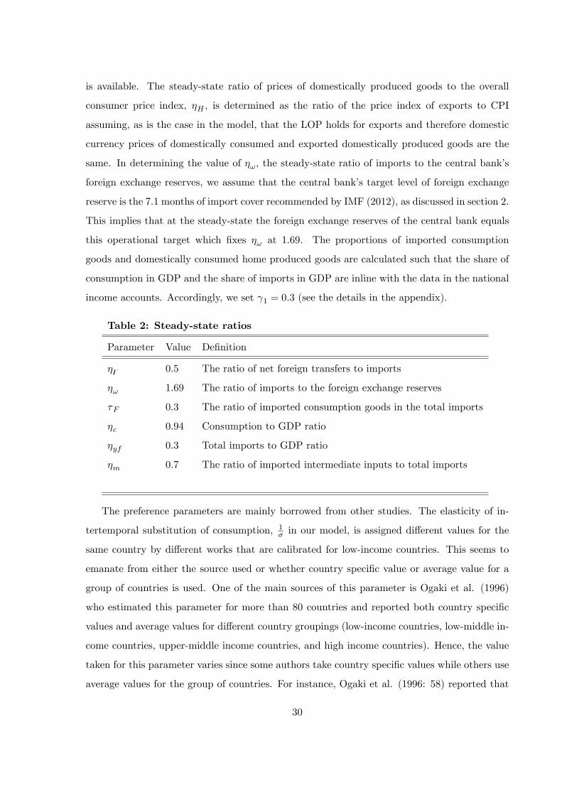
income accounts. Accordingly, we set 1 = 0:3 (see the details in the appendix).

Table 2: Steady-state ratios

Parameter Value De�nition

�z 0:5 The ratio of net foreign transfers to imports

�! 1:69 The ratio of imports to the foreign exchange reserves

�F 0:3 The ratio of imported consumption goods in the total imports

�c 0:94 Consumption to GDP ratio

�yf 0:3 Total imports to GDP ratio

�m 0:7 The ratio of imported intermediate inputs to total imports

The preference parameters are mainly borrowed from other studies. The elasticity of in-

tertemporal substitution of consumption, 1� in our model, is assigned di¤erent values for the

same country by di¤erent works that are calibrated for low-income countries. This seems to

emanate from either the source used or whether country speci�c value or average value for a

group of countries is used. One of the main sources of this parameter is Ogaki et al. (1996)

who estimated this parameter for more than 80 countries and reported both country speci�c

values and average values for di¤erent country groupings (low-income countries, low-middle in-

come countries, upper-middle income countries, and high income countries). Hence, the value

taken for this parameter varies since some authors take country speci�c values while others use

average values for the group of countries. For instance, Ogaki et al. (1996: 58) reported that

30

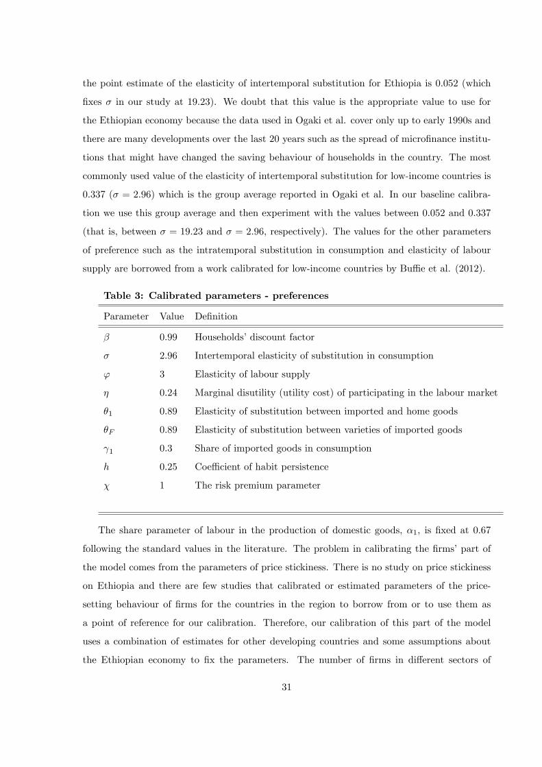
the point estimate of the elasticity of intertemporal substitution for Ethiopia is 0.052 (which

�xes � in our study at 19:23). We doubt that this value is the appropriate value to use for

the Ethiopian economy because the data used in Ogaki et al. cover only up to early 1990s and

there are many developments over the last 20 years such as the spread of micro�nance institu-

tions that might have changed the saving behaviour of households in the country. The most

commonly used value of the elasticity of intertemporal substitution for low-income countries is

0.337 (� = 2:96) which is the group average reported in Ogaki et al. In our baseline calibra-

tion we use this group average and then experiment with the values between 0.052 and 0.337

(that is, between � = 19:23 and � = 2:96, respectively). The values for the other parameters

of preference such as the intratemporal substitution in consumption and elasticity of labour

supply are borrowed from a work calibrated for low-income countries by Bu¢ e et al. (2012).

Table 3: Calibrated parameters - preferences

Parameter Value De�nition

� 0:99 Households�discount factor

� 2:96 Intertemporal elasticity of substitution in consumption

' 3 Elasticity of labour supply

� 0:24 Marginal disutility (utility cost) of participating in the labour market

�1 0:89 Elasticity of substitution between imported and home goods

�F 0:89 Elasticity of substitution between varieties of imported goods

1 0:3 Share of imported goods in consumption

h 0:25 Coe¢ cient of habit persistence

� 1 The risk premium parameter

The share parameter of labour in the production of domestic goods, �1, is �xed at 0:67

following the standard values in the literature. The problem in calibrating the �rms�part of

the model comes from the parameters of price stickiness. There is no study on price stickiness

on Ethiopia and there are few studies that calibrated or estimated parameters of the price-

setting behaviour of �rms for the countries in the region to borrow from or to use them as

a point of reference for our calibration. Therefore, our calibration of this part of the model

uses a combination of estimates for other developing countries and some assumptions about

the Ethiopian economy to �x the parameters. The number of �rms in di¤erent sectors of

31

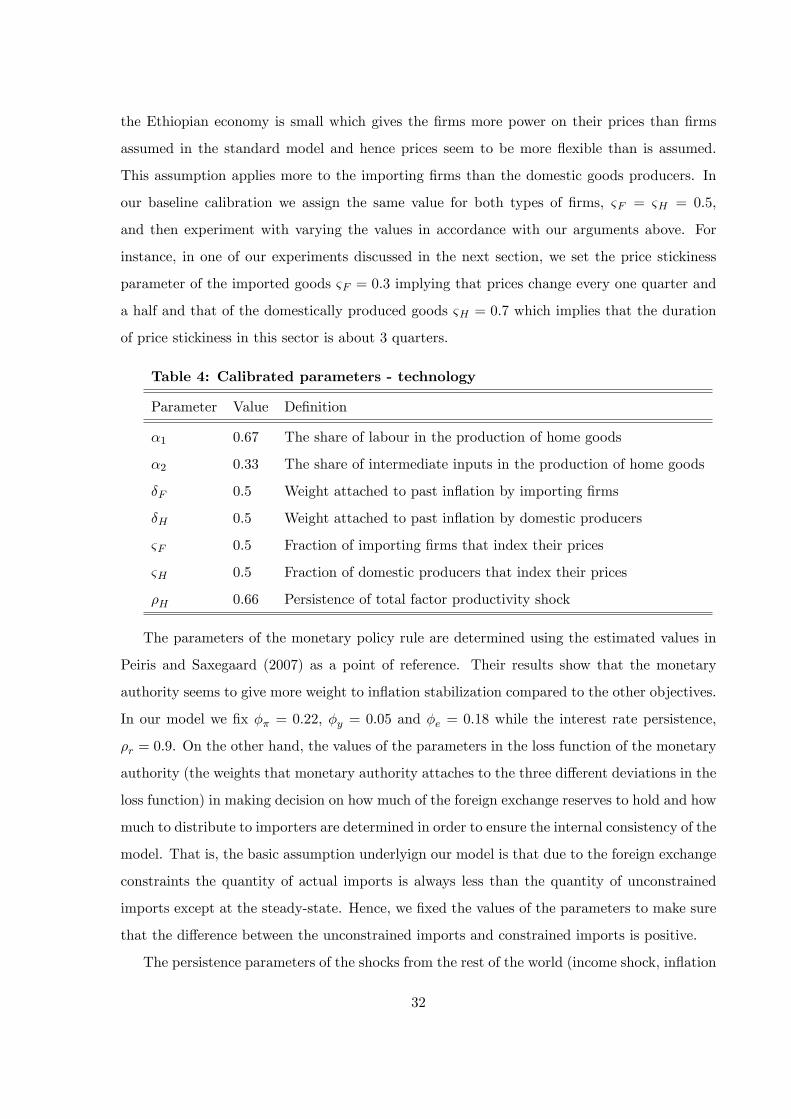
the Ethiopian economy is small which gives the �rms more power on their prices than �rms

assumed in the standard model and hence prices seem to be more �exible than is assumed.

This assumption applies more to the importing �rms than the domestic goods producers. In

our baseline calibration we assign the same value for both types of �rms, &F = &H = 0:5,

and then experiment with varying the values in accordance with our arguments above. For

instance, in one of our experiments discussed in the next section, we set the price stickiness

parameter of the imported goods &F = 0:3 implying that prices change every one quarter and

a half and that of the domestically produced goods &H = 0:7 which implies that the duration

of price stickiness in this sector is about 3 quarters.

Table 4: Calibrated parameters - technology

Parameter Value De�nition

�1 0:67 The share of labour in the production of home goods

�2 0:33 The share of intermediate inputs in the production of home goods

�F 0:5 Weight attached to past in�ation by importing �rms

�H 0:5 Weight attached to past in�ation by domestic producers

&F 0:5 Fraction of importing �rms that index their prices

&H 0:5 Fraction of domestic producers that index their prices

�H 0:66 Persistence of total factor productivity shock

The parameters of the monetary policy rule are determined using the estimated values in

Peiris and Saxegaard (2007) as a point of reference. Their results show that the monetary

authority seems to give more weight to in�ation stabilization compared to the other objectives.

In our model we �x �� = 0:22, �y = 0:05 and �e = 0:18 while the interest rate persistence,

�r = 0:9. On the other hand, the values of the parameters in the loss function of the monetary

authority (the weights that monetary authority attaches to the three di¤erent deviations in the

loss function) in making decision on how much of the foreign exchange reserves to hold and how

much to distribute to importers are determined in order to ensure the internal consistency of the

model. That is, the basic assumption underlyign our model is that due to the foreign exchange

constraints the quantity of actual imports is always less than the quantity of unconstrained

imports except at the steady-state. Hence, we �xed the values of the parameters to make sure

that the di¤erence between the unconstrained imports and constrained imports is positive.

The persistence parameters of the shocks from the rest of the world (income shock, in�ation

32

shock, and monetary policy shocks) are estimated from data. There are two alternatives to

estimate these parameters. The �rst is to generate the data for the rest of the world (world

minus Ethiopia) for each of the variables and estimate the parameters. The second alternative

is to estimate the parameters from the data for the OECD member countries. Though the

�rst alternative seems theoretically appealing, we believe that the second alternative is more

practical for two reasons. First, shocks from the OECD countries are more important for

Ethiopia since these are the countries with which Ethiopia has strong economic ties though

recent trends show the growing importance of emerging economies like China and India. Second,

the data for this group of countries is well organized and readily available for estimation.

Accordingly, we estimated the parameters from the annual data of OECD member countries

of the WDI-GDF for the period 1961-2011.

Table 5: Calibrated parameters- monetary policy and the rest of the world

Parameters Value De�nition

�r 0:9 Persistence of interest rate

�� 0:22 In�ation stabilization

�y 0:057 Output stabilization

�e 0:18 Exchange rate stabilization

�z 0:65 Persistence of shock to the net foreign transfers

� 3 The weight attached to deviations of end of period reserves from the target

�u 2:2 The weight put on the gap between unconstrained and constrained imports

�yf 1:22 The weight attached to import smoothing

�y� 0:54 Persistence of foreign income shock

��� 0:49 Persistence of foreign in�ation shock

�r� 0:51 Persistence of foreign interest rate shock

Using this baseline calibration we solved the log-linear approximation to the model and

simulated it for various domestic and external shocks.16 We made some experiments on how

the key macroeconomic variables of an economy that faces a foreign exchange constraint respond

to various shocks and how such a model di¤ers from the standard one. The results of these

simulation experiments are discussed below.

16The DYNARE toolbox (Adjemian et al. (2012)) is used to solve the model numerically and generate the

impulse response functions to di¤erent domestic and external shocks

33

5.2 Simulation results

Our main interest in this study is to understand how the introduction of foreign exchange

constraint to importers and the problem of foreign exchange rationing to central banks change

the dynamics of key macroeconomic variables compared to what is predicted by the standard

model. To this e¤ect, we solved and simulated both the model with the foreign exchange

constraint (the modi�ed model) and the model without the constraint (the standard model)

under the same parametrization and compared the behaviour of key macroeconomic variables

in response to various shocks.17 We consider shocks to productivity, domestic monetary policy,

net foreign transfers, terms of trade, foreign income, and foreign monetary policy. All shocks

are temporary and of the same magnitude. Since we solved and simulated the log-linear ap-

proximation to the original models, the �gures presented below show the percentage deviations

of the variables from their respective steady-states.18

Before the discussion of the comparison of the two models, however, we would like to

indicate one interesting feature of the modi�ed model. Given the foreign exchange constraint,

the standard Taylor type monetary policy rule, and the parametrization we used, monetary

policy leads to opposite and signi�cant e¤ects compared to what is predicted by the standard

model. To be speci�c, contractionary monetary policy leads to expansion of consumption

and output and contraction of employment in the modi�ed model. This is more so specially if

importing �rms can reoptimize their prices more frequently than the domestic producers. That

is, if the duration of the price stickiness in the import sector is shorter than that of the domestic

goods prices, the expansionary e¤ect of the contractionary monetary policy will be ampli�ed.

In our baseline calibration we assumed that both types of �rms face the same duration of

price stickiness, &F = &H = 0:5. As can be seen from Figure 4, decreasing the duration of

price stickiness for importing �rms to &F = 0:3 and increasing that of domestic goods prices to

&H = 0:7 leads the contractionay monetary policy to have more ampli�ed expansionary e¤ects

on output and consumption and contractionary e¤ects on employment.

17The two models are solved and simulated for the same parameters discussed in the calibration process above

except for risk premium parameter, �. In the modi�ed model we assigned this parameter a value that is used in

literature on low-income countries. In the standard model we assigned relatively larger value in order to solve

and obtain reasonable impulse responses of the model while keeping all the other parameters the same.18See the derivation of some model equations, steady-state conditions, and the details of the log-linear ap-

proximation to the model in the Appendix.

34

Figure 4: Impulse responses to a monetary policy shock with varying degree of price stickiness

0 2 4 6 8 100

0.2

0.4

0.6

0.8

1

1.2

1.4Income

Years

%ag

e de

viat

ions

 from

 SS

Both 0.50.3 and 0.7

0 2 4 6 8 100.2

0.4

0.6

0.8

1

1.2Consumption

Years

%ag

e de

viat

ions

 from

 SS

Both 0.50.3 and 0.7

0 2 4 6 8 10­0.24

­0.22

­0.2

­0.18

­0.16

­0.14

­0.12

­0.1

­0.08

­0.06Employment

Years

%ag

e de

viat

ions

 from

 SS

Both 0.50.3 and 0.7

0 2 4 6 8 100

0.2

0.4

0.6

0.8

1

1.2

1.4

1.6Marginal cost

Years

%ag

e de

viat

ions

 from

 SS

Both 0.50.3 and 0.7

0 2 4 6 8 10

0.7

0.8

0.9

1

1.1

1.2

1.3

1.4Inflation

Years

%ag

e de

viat

ions

 from

 SS

Both 0.50.3 and 0.7

As indicated in the discussion of the calibration of the model, there is no macro or micro-

econometric study on price stickiness in the Ethiopian economy. However, given the structure

of the economy and the number of �rms in the domestic production and the import sectors

it seems that the �rms in the latter sector experience more frequent price resetting. If this is

the case, contractionary monetary policy leads to expansion of output and consumption since

imports of both consumption goods and intermediate inputs will be reltively cheaper. The

contraction in employment seems to result from input substitution by domestic �rms. That

is, when imported intermediate inputs become relatively cheaper, depending on the degree of

substitutability between inputs, �rms employ more of the now cheaper input and decrease the

employment of others. This can be the case in our model since we assume that the labour

market is competitive and �rms can adjust their employment of labour easily. We will discuss

the details of the mechanisms of this shock when we compare the two models in Figure 6 below.

Next we present the comparison between the two models. One feature that is clearly

observable when comparing the two models is that the modi�ed model generates more variations

in most of the variables considered than the standard model. This is in line with the stylized

35

Figure 5: Impulse responses to a productivity shock

0 2 4 6 8 100

0.5

1

1.5

2

2.5Income

Years

%ag

e de

viat

ions

 from

 SS

modifiedstandard

0 2 4 6 8 10­0.5

0

0.5

1

1.5

2Consumption

Years

%ag

e de

viat

ions

 from

 SS

modifiedstandard

0 2 4 6 8 10­0.7

­0.6

­0.5

­0.4

­0.3

­0.2

­0.1

0

0.1

0.2Employment

Years

%ag

e de

viat

ions

 from

 SS

modifiedstandard

0 2 4 6 8 10­0.8

­0.6

­0.4

­0.2

0

0.2

0.4

0.6

0.8

1Marginal cost

Years

%ag

e de

viat

ions

 from

 SS

modifiedstandard

0 2 4 6 8 100

0.2

0.4

0.6

0.8

1Inflation

Years

%ag

e de

viat

ions

 from

 SS

modifiedstandard

facts about the behaviour of macroeconomic variables of low-income countries like Ethiopia.

For instance, according to Stiglitz et al. (2006: 57) one of the di¤erences in macroeconomic

behavior between developed and developing countries is that the latter are �less able to absorb

shocks, and the structures of their economies are more likely to amplify shocks than dampen

them� which is vividly observable in the impulse response presented in Figures 5-10. This

vulnerability of low-income countries to shocks and their inability to absorb the shocks are

discussed in many works (see, among others, Collier and Gunning (1999), Kose and Reizman

(2001), Cashin et al. (2004)).

The key macroeconomic variables we considered show the same behaviour in response to

a total factor productivity shock, as shown in Figure 5. The direction of the e¤ect of a

productivity shock is the same for both models but the magnitude is more pronounced for

the modi�ed model. The only exception is the marginal cost that behaves in an opposite

way in the two models. In the standard model it is expected that an increase in productivity

results into expansion of output and consumption and contraction of employment initially.19

19Note that it is not always the case that productivity shock leads to expansions. For example, Basu et al.

36

Figure 6: Impulse responses to a domestic monetary policy shock

0 2 4 6 8 10­0.1

0

0.1

0.2

0.3

0.4

0.5

0.6Income

Years

%ag

e de

viat

ions

 from

 SS

modifiedstandard

0 2 4 6 8 10­0.4

­0.2

0

0.2

0.4

0.6Consumption

Years

%ag

e de

viat

ions

 from

 SS

modifiedstandard

0 2 4 6 8 10­0.15

­0.1

­0.05

0

0.05

0.1

0.15

0.2

0.25Employment

Years

%ag

e de

viat

ions

 from

 SS

modifiedstandard

0 2 4 6 8 10­0.1

0

0.1

0.2

0.3

0.4

0.5

0.6

0.7Marginal cost

Years

%ag

e de

viat

ions

 from

 SS

modifiedstandard

0 2 4 6 8 100.5

0.6

0.7

0.8

0.9

1

1.1

1.2

1.3Inflation

Years

%ag

e de

viat

ions

 from

 SS

modifiedstandard

The increased productivity also decreases marginal costs. Furthermore, due to the decreasing

marginal costs there is a tendency for the domestic economy to experience de�ationary pressure.

In the modi�ed model, however, marginal costs increase in response to a positive productivity

shock. This can happen only if the negative e¤ect of the increasing productivity on marginal

costs is more than o¤set by its positive e¤ect on the terms of trade which makes import of

intermediate goods more expensive relative to the price of domestically produced goods and

hence increase the marginal costs of production. This will also put upward pressure on the

real exchange rate which increases cost of production and overall in�ation at which stage the

monetary authority�s intervention leads the economy to its steady-state.

The e¤ect of a domestic monetary policy shock is opposite to what is expected in the stan-

dard model, as discussed in the beginning of this section and illustrated in Figure 4 above.

Figure 6 shows the impulse responses to a domestic monetary policy shock in the two models.

The standard model shows the conventional results of contractionary monetary policy where

(2006) report that the initial impact of an improvement in productivity could be contractionary when �rms

cannot adjust their prices in a sticky price model.

37

all output, consumption, employment, marginal cost, and in�ation fall at least initially; that

is contractionary monetary policy does what its name implies. Economic theory indicates

that there are two channels through which the contractionary monetary policy shock a¤ects

macroeconomic variables of an open economy. First, an increasing interest rate leads to ap-

preciation of the nominal exchange rate which leads the real exchange rate to appreciate since

the domestic price index adjusts slowly. The appreciation of the real exchange rate leads to

a decreasing demand for domestic tradable goods by foreigners (that is, exports of the home

country decrease). On the other hand, the same event (that is, the appreciation of the exchange

rate of the home country) makes imports cheaper relative to home produced goods which leads

to an increasing demand for imports by domestic consumers. These decreasing exports and

increasing imports reinforce each other and lead to a decreasing domestic income.

The second channel through which the monetary policy shock a¤ects the economy is through

the e¤ect of the interest rate on households�expenditure. That is, an increasing interest rate

encourages domestic consumers to postpone their current consumption depending on the re-

sponsiveness of savings to changes in interest rates. The e¤ects through both channels augment

each other in reducing output and, therefore, consumption.

In the modi�ed model, however, appreciation of domestic currency makes imports of con-

sumption goods and intermediate inputs cheaper which leads to expansionary e¤ects. Depend-

ing on the degrees of substitution between labour and intermediate inputs, employment might

decrease as can be seen in both Figures 4 and 6.

The shocks to net foreign transfers lead to conventional results under both circumstances

though the magnitudes are di¤erent. The e¤ects of net foreign transfer is magni�ed in the

modi�ed model since increasing net foreign transfers leads to increasing availability of foreign

exchange for imports of both consumption goods and intermediate inputs.

As de�ned in our model, increasing terms of trade is deterioration of the terms of trade

for the domestic economy since it implies that the prices of imports are increasing relative to

the prices of exports. This deterioration of the terms of trade leads to decreasing capacity of

the economy to import and hence has a contractionary e¤ect on the domestic economy. In the

modi�ed model the e¤ects are magni�ed, as can be seen from Figure 8, due to the link of the

deterioration of the terms of trade to the foreign exchange constraints.

Figure 9 shows the responses of the key macroeconomic variables to a foreign income shock.

The responses of output, consumption, employment, and marginal costs to the shocks in foreign

38

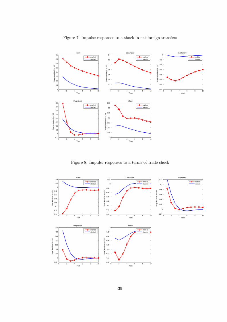
Figure 7: Impulse responses to a shock in net foreign transfers

0 2 4 6 8 100

0.1

0.2

0.3

0.4

0.5

0.6

0.7

0.8Income

Years

%ag

e de

viat

ions

 from

 SS

modifiedstandard

0 2 4 6 8 100

0.2

0.4

0.6

0.8

1

1.2

1.4Consumption

Years

%ag

e de

viat

ions

 from

 SS

modifiedstandard

0 2 4 6 8 10­0.7

­0.6

­0.5

­0.4

­0.3

­0.2

­0.1

0Employment

Years

%ag

e de

viat

ions

 from

 SS

modifiedstandard

0 2 4 6 8 10­0.1

0

0.1

0.2

0.3

0.4

0.5

0.6

0.7

0.8Marginal cost

Years

%ag

e de

viat

ions

 from

 SS

modifiedstandard

0 2 4 6 8 100

0.05

0.1

0.15

0.2

0.25

0.3

0.35Inflation

Years

%ag

e de

viat

ions

 from

 SS

modifiedstandard

Figure 8: Impulse responses to a terms of trade shock

0 2 4 6 8 10­0.14

­0.12

­0.1

­0.08

­0.06

­0.04

­0.02

0

0.02

0.04Income

Years

%ag

e de

viat

ions

 from

 SS

modifiedstandard

0 2 4 6 8 10­0.14

­0.12

­0.1

­0.08

­0.06

­0.04

­0.02

0

0.02Consumption

Years

%ag

e de

viat

ions

 from

 SS

modifiedstandard

0 2 4 6 8 10­0.02

0

0.02

0.04

0.06

0.08

0.1

0.12Employment

Years

%ag

e de

viat

ions

 from

 SS

modifiedstandard

0 2 4 6 8 10­0.05

0

0.05

0.1

0.15

0.2

0.25

0.3

0.35Marginal cost

Years

%ag

e de

viat

ions

 from

 SS

modifiedstandard

0 2 4 6 8 10­0.16

­0.14

­0.12

­0.1

­0.08

­0.06

­0.04

­0.02

0Inflation

Years

%ag

e de

viat

ions

 from

 SS

modifiedstandard

39

Figure 9: Impulse responses to a foreign income shock

0 2 4 6 8 10­0.4

­0.3

­0.2

­0.1

0

0.1

0.2

0.3Income

Years

%ag

e de

viat

ions

 from

 SS

modifiedstandard

0 2 4 6 8 100

0.05

0.1

0.15

0.2

0.25

0.3

0.35Consumption

Years

%ag

e de

viat

ions

 from

 SS

modifiedstandard

0 2 4 6 8 10­0.25

­0.2

­0.15

­0.1

­0.05

0

0.05

0.1Employment

Years

%ag

e de

viat

ions

 from

 SS

modifiedstandard

0 2 4 6 8 10­0.4

­0.3

­0.2

­0.1

0

0.1

0.2

0.3Marginal cost

Years

%ag

e de

viat

ions

 from

 SS

modifiedstandard

0 2 4 6 8 10­0.5

­0.4

­0.3

­0.2

­0.1

0

0.1

0.2Inflation

Years

%ag

e de

viat

ions

 from

 SS

modifiedstandard

income are di¤erent in the two models. In the standard model all of the 4 variables show

expansion at least initially due to this shock. This is so since in the standard model an increasing

foreign income a¤ects domestic output and consumption through an increasing demand for the

domestic exports and through the international risk sharing, respectively. In the modi�ed

model, however, all of the 4 variables show contraction at least initially due to the shock

in foreign income. This seemingly counterintuitive result may be explained as follows. The

increasing foreign income is expected to increase domestic income only if its direct e¤ect through

an increasing demand for domestic exports and increasing domestic income and consumption

through the international risk sharing is greater than its indirect e¤ect through the terms of

trade. All other things remaining the same, increasing foreign income leads to an increasing

demand for goods and services by households of the rest of the world that leads to increasing

foreign price levels which translate into increasing costs of imports of consumption goods and

intermediate inputs for the domestic economy. This indirect e¤ect is stronger in the modi�ed

model due to the foreign exchange constraints.

The two models seem to show signi�cantly di¤erent impulse responses to a foreign mone-

40

Figure 10: Impulse responses to a foreign monetary policy shock

0 2 4 6 8 10­1.2

­1

­0.8

­0.6

­0.4

­0.2

0

0.2Income

Years

%ag

e de

viat

ions

 from

 SS

modifiedstandard

0 2 4 6 8 10­1

­0.8

­0.6

­0.4

­0.2

0

0.2

0.4Consumption

Years

%ag

e de

viat

ions

 from

 SS

modifiedstandard

0 2 4 6 8 10­0.02

0

0.02

0.04

0.06

0.08Employment

Years

%ag

e de

viat

ions

 from

 SS

modifiedstandard

0 2 4 6 8 10­1.4

­1.2

­1

­0.8

­0.6

­0.4

­0.2

0

0.2Marginal cost

Years

%ag

e de

viat

ions

 from

 SS

modifiedstandard

0 2 4 6 8 10­1.2

­1

­0.8

­0.6

­0.4

­0.2

0

0.2Inflation

Years

%ag

e de

viat

ions

 from

 SS

modifiedstandard

tary policy shock as can be seen from Figure 10. In the standard model we expect that at least

consumption responds positively to a contractionary monetary policy in the rest of the world

due to the international risk sharing since we assumed that the economy has access to inter-

national �nancial markets though this access is imperfect or limited. In the modi�ed model,

an increasing foreign interest rate (say due to tight monetary policy) causes the domestic cur-

rency to depreciate which increases the cost of imported consumption goods and intermediate

inputs. As a result, import falls which, in turn, leads to a fall in both domestic income and

consumption.

6 Conclusions

In this paper we formalized the argument that the availability of foreign exchange is one of

the crucial factors that determine economic activity in developing countries. Many studies

documented that the shortage of foreign exchange to import capital and intermediate inputs

results into decreasing investment and fall in growth of GDP in these countries. This emanates

41

from the heavy reliance of these economies on imported capital and intermediate inputs. These

imports, in turn, depend on the availability and cost of foreign exchange at the disposal of the

economy. Hence, the performance of the external sector of the economy in generating foreign

exchange is critical to the performance of the rest of the macroeconomy of these countries. As

a result, in the event of a global �nancial crisis that a¤ects the actual or expected in�ow of

foreign exchange these economies are expected to be hard-hit.

It is worth mentioning that unlike other constraints such as credit constraints for investment

or for working capital that policy makers may address via various policy instruments, the foreign

exchange constraints cannot be alleviated in the short-run. Only the change in the structure

or the change in the natural resource base of the economy can change the severity of this

constraint. Therefore, understanding the behaviour of the macroeconomy of these countries

in response to various domestic and global shocks requires introducing the foreign exchange

constraints into the models that are meant to be applied to these economies. In this study we

introduced a foreign exchange constraint that importing �rms face and the problem of foreign

exchange reserve management that the monetary authority faces in such economies into a small

open economy New Keynesian DSGE model. Therefore, the main contribution of this study,

as a �rst study to incorporate a foreign exchange constraint into a DSGE model, is enhancing

our understanding of the macroeconomic dynamics of countries that face this constraint.

It is important to emphasize again that calibration of the model to the Ethiopian economy

is problematic as it is the case for many low-income countries. For some variables there are

no macro or microeconometric studies from which the parameter values could be borrowed or

there are no relevant data from which the parameters can be estimated. We made e¤orts to

make the calibration of parameters as reasonable as possible and hence we believe that the

analysis based on the parameters above su¢ ces to the objective of the study and there are

some interesting results from our simulation experiments which we summarize below.

As we indicated in the introductory section and in the survey of related literature, conven-

tional policy instruments may have di¤erent, and sometimes opposite, e¤ects when applied to

the economies of low-income countries. One of the �ndings of our simulation experiments con-

curs with this argument. That is, in the model with the foreign exchange constraints monetary

policy exhibits an opposite e¤ect compared to what is expected in the standard model. This

e¤ect is more pronounced with the relative degree of price stickiness of the imported and do-

mestically produced goods. For instance, as illustrated in the text, with shorter duration of the

42

price rigidity of the import sector relative to the domestic goods sector, which we believe is the

case for countries like Ethiopia, contractionary monetary policy will have strong expansionary

e¤ect.

Furthermore, the comparison of impulse response functions of the modi�ed model and of

the standard model shows that the modi�ed model generates more variability in most of the

key macroeconomic variables considered when hit by the same domestic and external shocks.

This result corresponds with the stylized facts about the behaviour of the key macroeconomic

variables of low-income countries in an event of shocks.

Finally, the model in this paper can easily be extended to incorporate the bias of a monetary

authority in the allocation of the available foreign exchange to importers of consumption goods

and intermediate inputs. This can be done by modeling the importers of consumption goods and

intermediate inputs separately and experiment on the e¤ects of the changes on the distribution

of the available foreign exchange reserves to the two types of imports on the key macroeconomic

variables.

References

[1] Adam, Christopher, Stephen O�Connell, and Edward Bu¢ e (2008) Aid volatility, monetary

policy rules and the capital account in African economies. World Economy & Finance

Research Programme, Birkbeck, University of London. Working Paper Series WEF 0037.

[2] Adam, Christopher, Stephen O�Connell, Edward Bu¢ e, and Catherine Pattillo (2009)

Monetary Policy Rules for Managing Aid Surges in Africa. Review of Development Eco-

nomics, Vol. 13, No. 3: 464�490.

[3] Adjemian, Stephane, Houtan Bastani, Michel Juillard, Ferhat Mihoubi, George Perendia,

Marco Ratto, and Sebastien Villemot (2012) Dynare: Reference Manual Version 4. Dynare

Working Papers Series, Working Paper no. 1.

[4] Adolfson, Malin, Stefan Laséen , Jesper Lindé, and Mattias Villani (2005) Bayesian esti-

mation of an open economy DSGE model with incomplete pass-through. Sveriges Riksbank

Working paper 179.

43

[5] Adolfson, Malin, Stefan Laséen , Jesper Lindé, and Mattias Villani (2007) Bayesian es-

timation of an open economy DSGE model with incomplete pass-through. Journal of

International Economics, 72: 481�511.

[6] Agenor, P.R. and P.J. Montiel (2008) Development Macroeconomics, 3rd ed. Princeton

University Press.

[7] Basu, Susanto, John G. Fernald, and Miles S. Kimball (2006) Are Technology Improve-

ments Contractionary? The American Economic Review, Vol. 96, No. 5: 1418-1448.

[8] Bäurle and Menz (2008) Monetary Policy in a Small Open Economy Model: A DSGE-VAR

Approach for Switzerland, Study Center Gerzensee, Working Paper 08.03.

[9] Benigno, Pierpaolo (2001) Price Stability with Imperfect Financial Integration. CEPR

Discussion Paper No. 2854.

[10] Bu¢ e, Edward E., Andrew Berg, Catherine Pattillo, Rafael Portillo, and Luis-Felipe Zanna

(2012) Public Investment, Growth, and Debt Sustainability: Putting Together the Pieces.

IMF Working Paper, WP/12/144.

[11] Bulir, Ales and Javier Hamann (2003) Aid Volatility: An Empirical Assessment. IMF Sta¤

Papers, Vol 50, No.1: 64-89.

[12] Bulir, Ales and Javier Hamann (2008) Volatility of Development Aid: From the Frying

Pan into the Fire? World Development, Vol.36, No.10: 2048�2066.

[13] Calvo, Guillermo A. (1983) Staggered prices in a utility-maximizing framework. Journal

of Monetary Economics, Vol. 12, No. 3: 383-98.

[14] Cashin, Paul, C. John McDermott, and Catherine Pattillo (2004) Terms of trade shocks

in Africa: are they short-lived or long-lived? Journal of Development Economics 73: 727�

744.

[15] Chenery, Hollis B. and Michael Bruno (1962) Development Alternatives in an Open Econ-

omy: The Case of Israel. The Economic Journal, Vol. 72, No. 285: 79-103.

[16] Christiano, Lawrence J., Mathias Trabandt, and Karl Walentin (2011a) Introducing Finan-

cial Frictions and Unemployment into a Small Open Economy Model. Journal of Economic

Dynamics & Control, 35: 1999�2041.

44

[17] Collier, Paul and Jan Willem Gunning (1999) Explaining African Economic Performance.

Journal of Economic Literature, Vol. 37, No. 1: 64-111.

[18] Dorosh, Paul, Sherman Robinson and Hashim Ahmed (2009) Economic Implications of

Foreign Exchange Rationing in Ethiopia. Development Strategy and Governance Division,

International Food Policy Research Institute � Ethiopia Strategy Support Program 2,

Ethiopia. Discussion Paper No. ESSP2 009.

[19] Emran, M. Shahe and Forhad Shilpi (1996) Foreign exchange rationing and the aggregate

import demand function. Economics Letters, 51: 315-322.

[20] Fafchamps, Marcel (2004) Market Institutions in Sub-Saharan Africa: Theory and Evi-

dence. The MIT Press.

[21] Gali, Jordi and Tommaso Monacelli (2005) Monetary Policy and Exchange Rate Volatility

in a Small Open Economy. Review of Economic Studies 72: 707�734.

[22] Hemphill, William L. (1974) The e¤ect of foreign exchange receipts on imports of less

developed countries. IMF Sta¤ Papers, Vol. 21, No. 3: 637-677.

[23] Houssa, Romain, Christopher Otrok, and Radu Puslenghe (2010) A Model for Monetary

Policy Analysis for Sub-Saharan Africa. Open Econ Rev. 21: 127-145, Springer Science +

Business Media, LLC 2009.

[24] IMF (2012) The Federal Democratic Republic of Ethiopia Sta¤Report for the 2012 Article

IV Consultation. http://www.imf.org/external/pubs/ft/scr/2012/cr12287.pdf.

[25] Justiniano and Preston (2010a) Can structural small open-economy models account for

the in�uence of foreign disturbances? Journal of International Economics, 81: 61�74 and

[26] Justiniano, Alejandro and Bruce Preston (2010b) Monetary policy and uncertainty in an

empirical small open-economy model. Journal of Applied Econometrics, 25: 93-128.

[27] Khan, Mohsin S. and Malcolm D. Knight (1988) Important Compression and Export

Performance in Developing Countries. The Review of Economics and Statistics, Vol. 70,

No. 2: 315-321.

[28] Kose, M. Ayhan and Raymond Riezman (2001) Trade shocks and macroeconomic �uctu-

ations in Africa. Journal of Development Economics, Vol. 65: 55�80.

45

[29] Kose, M. Ayhan (2002) Explaining business cycles in small open economies �How much

do world prices matter?� Journal of International Economics, 56: 299�327.

[30] Lensink, Robert (1995) Foreign exchange constraints and developing countries. Economic

Modelling, Vol. 12, No. 2: 179-191.

[31] Marquez, Jaime (1985) Foreign exchange constraints and growth possibilities in the LDCs.

Journal of Development Economics, 19: 39-57.

[32] McKinnon, Ronald I. (1964) Foreign Exchange Constraints in Economic Development and

E¢ cient Aid Allocation. The Economic Journal, Vol. 74, No. 294: 388-409.

[33] Mishra, Prachi and Peter Montiel (2012) How e¤ective is monetary transmission in low-

income countries? A survey of empirical evidence. IMF Working paper, WP/12/143.

[34] Mishra, Prachi, Peter J. Montiel and Antonio Spilimbergo (2012) Monetary transmission

in low-income countries: E¤ectiveness and policy implications. IMF Economic Review,

Vol. 60, No. 2: 270-302.

[35] Monacelli, Tommaso (2005) Monetary policy in a low pass-through environment. Journal

of Money, Credit and Banking 37: 1047�1066.

[36] Moran, Cristian (1989) Import under a Foreign Exchange Constraint. The World Bank

Economic Review, Vol. 3, No. 2: 279-295.

[37] Ogaki, Masao, Jonathan D. Ostry, and Carmen M. Reinhart (1996) Saving Behavior in

Low- and Middle-Income Developing Countries: A Comparison. IMF Sta¤ Papers, Vol.

43, No. 1: 38-71.

[38] Peiris, Shanaka J. and Magnus Saxegaard (2007) An Estimated DSGE Model for Monetary

Policy Analysis in Low-Income Countries. IMF Working Paper, WP/07/282.

[39] Polterovich, Victor and Vladimir Popov (2003) Accumulation of Foreign Ex-

change Reserves and Long Term Growth. http://www.nes.ru/english/about/10th-

Anniversary/papers-pdf/Popov-Polterovich.pdf.

[40] Porter, R. and S. Ranney (1982) An Eclectic Model of Recent LDC Macroeconomic Policy

Analysis. World Development, Vol. 10 No. 9: 751-765.

46

[41] Schmitt-Grohe, Stephanie and Martin Uribe (2003) Closing small open economy models.

Journal of International Economics 61: 163-185.

[42] Stiglitz, Joseph E., Jose Antonio Ocampo, Shari Spiegel, Ricardo Ffrench-Davis, and

Deepak Nayyar (2006) Stability with Growth: Macroeconomics, Liberalization, and Devel-

opment. Oxford University Press.

[43] United Nations (2012) UNCTAD Handbook of statistics 2012.

http://unctad.org/en/PublicationsLibrary/tdstat37_en.pdf.

[44] Worrell, DeLisle (2012) Policies for stabilization and growth in small very open economies.

The Group of Thirty, Occasional Paper 85.

[45] Wyplosz, Charles (2007) The Foreign Exchange Reserves Buildup: Business as Usual?

Paper presented on Workshop on Debt, Finance and Emerging Issues in Financial Inte-

gration, 6-7 March 2007, Commonwealth Secretariat, Marlborough House, London.

47

7 Appendix

In this appendix we provide the derivation of some key relationships, steady-state conditions,

and the log-linear approximation to the model. We log-linearized the equations that char-

acterize the equilibrium conditions around a steady-state to solve and simulate the model.

For most of the variables in the model the log deviation is represented by lower-cases, i.e.,

xt � lnXt � lnX where X is the steady state value of Xt. For some variables we used a

variable with a hat to represent the log-deviation, i.e., b!t = ln!t � ln! where ! is the steadystate value of !t. The log-linearized approximation to the model is given by equations (43-70)

below.

7.0.1 Households

The households�labour supply condition (the equality between the real wage and the marginal

rate of substitution of consumption for leisure) can be rewritten as

� (Lt)' (Ct � hCt�1)� Pt =Wt

which can be log-linearized

wt � pt = 'lt +�

(1� h)ct �h�

(1� h)ct�1 (43)

The consumption Euler equation (the households� optimal intertemporal allocation of con-

sumption) given by

�Et(Ct+1 � hCt)��

(Ct � hCt�1)��PtPt+1

=1

Rt

can be rewritten as

Rt = �Et(Ct+1 � hCt)�

(Ct � hCt�1)�Pt+1Pt

and can be log-linearized to yield

ct =1

1 + hEtct+1 +

h

1 + hct�1 �

(1� h)� (1 + h)

(rt � Et�t+1) (44)

Likewise, the households�optimality condition of asset holdings (the optimal holdings of do-

mestic and foreign bonds)

�Et�t+1Rt = �Et�t+1"t+1"t

R�t�t+1

48

which implies that

rt � Et�t+1 = r�t � Et��t+1 + Et�qt+1 + ln�t+1 � ln�

where �t is the risk-premium that households are required to pay on their foreign debt and is

given by

�t = exp [�� (at�1 +$t)]

where

at�1 ="t�1B�t�1Y FPt�1

Y F is the steady-state level of import and $t is the risk-premium shock. What is ln�t+1� ln�?

From the de�nition of �t we have

ln�t+1 = ��at � �$t+1

ln�t+1 � ln� = ��at � "rps;t

This implies that

rt � Et�t+1 = r�t � Et��t+1 + Et�qt+1 � �at � "rps;t (45)

where, as will be de�ned below, qt is the real exchange rate in its log-deviation, �t = lnPt �

lnPt�1 is the domestic rate of in�ation, and ��t = lnPt � lnPt�1 is the rate of in�ation in the

rest of the world.

Equations (43), (44), and (45) represent the log-linear approximations to the equilibrium

conditions of the household section. Before moving to the �rms section we introduce certain

relationships that will help the derivations that will follow.

7.0.2 Real Exchange rate, terms of trade, and other relationships

Log-linearizing the Law of One Price Gap, t ="tP �tPF;t

, around the symmetric steady-state

(simultaneous steady-state at both the domestic economy and the economy of the rest of the

world) we have

t = et + p�t � pF;t

and subtracting one period lag we obtain the following

t � t�1 = et � et�1 + ��t � �F;t (46)

49

Similarly, log-linearizing the real exchange rate, Qt ="tP �tPt, yields

qt = et + p�t � pt

We know that pt = (1� 1) pH;t + 1pF;t and from the de�nition of the Law of One Price

Gap (in log-linearized form) we have et + p�t = t + pF;t. Using these pieces, the log-linearized

equation of the real exchange rate can be rewritten as

qt = t + pF;t � [(1� 1) pH;t + 1pF;t]

qt = t + (pF;t � pH;t)� 1 (pF;t � pH;t)

From the de�nition of the terms-of-trade Vt =PF;tPH;t

, we have

vt = pF;t � pH;t

Employing the above de�nition of the terms of trade we obtain the following log-linearized

equation of the real exchange rate

qt = t + (1� 1) vt (47)

On the other hand, the evolution of the terms of trade is given by

vt = vt�1 + �F;t � �H;t + �tot;t (48)

where �tot;t is the terms of trade shock.

7.0.3 Firms

The New Keynesian Phillips Curves in this model are identical to those derived in Justiniano

and Preston (2010a and 2010b). The only di¤erence is the marginal costs in the New Keynesian

Phillips curve of the imported goods. In the present paper the marginal cost takes into account

the foreign exchange constraint through the Lagrangian multiplier as indicated below.

Home produced goods in�ation The equation of domestically produced goods in�ation

(the New Keynesian Phillips curve of home goods) is given by

�H;t � �H�H;t�1 = �Et (�H;t+1 � �H�H;t) + �HmcH;t (49)

50

where

�H =(1� &H) (1� &H�)

&H

Real marginal costs of the domestically produced goods is given by

MCH;t =

"��2�1

��1+

��2�1

���2# P�2F;tW�1t Z�1H;tPt

which can be log-linearized to yield

mcH;t = �1wt + �2pF;t � pt � zH;t

From the households�labour supply condition, assuming that the labour market is in equilib-

rium, we have

wt = pt + 'lt +�

(1� h)ct �h�

(1� h)ct�1

substituting into the real marginal cost equation we have

mcH;t = �1

�pt + 'lt +

�

(1� h)ct �h�

(1� h)ct�1�+ �2pF;t � pt � zH;t

mcH;t = �1

�'lt +

�

(1� h)ct �h�

(1� h)ct�1�+ �2pF;t + �1pt � pt � zH;t

mcH;t = �1

�'lt +

�

(1� h)ct �h�

(1� h)ct�1�+ �2pF;t � (1� �1) pt � zH;t

mcH;t = �1

�'lt +

�

(1� h)ct �h�

(1� h)ct�1�+ �2pF;t � �2pt � zH;t

we know that

pF;t � pt = pF;t � (1� 1) pH;t � 1pF;t

= (pF;t � pH;t)� 1 (pF;t � pH;t)

= (1� 1) vt

This implies that the real marginal cost of the home produced goods is given by

mcH;t = �1

�'lt +

�

(1� h)ct �h�

(1� h)ct�1�+ �2 (1� 1) vt � zH;t (50)

Importing Firms As discussed in the text, the importing �rms face foreign exchange con-

straints and their optimal price is given by

PF;t (i) =�F

(�F � 1)"tP

�t

�1 + �F;t

�51

The imported goods in�ation The New Keynesian Phillips curve of the importing �rms

is given by

�F;t � �F�F;t�1 = �Et (�F;t+1 � �F�F;t) + �F (mcF;t � pF;t) (51)

where

�F =(1� &F ) (1� &F�)

&F

and from the optimal mark-up price of the importing �rms we know that the marginal cost of

the importing �rms is given by

MCF;t = "tP�t (1 + �t)

After log-linearizing we have

et + p�t +

b�t(mcF;t � pF;t) =

�et + p

�t +

b�t�� pF;t = t +b�t

Note that when �rms do not face a foreign exchange constraint, we have only t - the law of

one price gap. As a result of the foreign exchange constraint that importing �rms face we have

additional term, b�t.Since the demand curve that the �rm faces remains the same with and without the foreign

exchange constraint, the ratio YF;t= (PF;t)��F for YF;t (i) importing �rm remain the same with

and without the foreign exchange constraint. This implies the following relationship between

the ratio of constrained to unconstrained imports and the Lagrangian multiplier of the foreign

exchange constraints

YF;t (i)

YF;t (i)u =

�PF;t(i)PF;t

���FYF;t�

(PF;t(i))u

(PF;t)u

���F(YF;t)

u

=

�PF;t (i)

(PF;t (i))u

���F (PF;t)u(YF;t)

u

��F YF;t

P��FF;t

�F;t =�1 + �F;t

���F ((PF;t)u)��F(YF;t)

uYF;t

(PF;t)��F

�F;t =�1 + �F;t

���F�F;t =

�1 + �F;t

���F(�F;t)

�1�F =

�1 + �F;t

�which can be log-linearized to yield

b�F;t = 1

�F((yF;t)

u � yF;t) (52)

52

7.0.4 Market clearing conditions

The goods market clearing condition (the resource constraint)

Yt = CH;t + C�H;t

can be log-linearized as

Y yt = CHcH;t + C�Hc

�H;t

where

cH;t = ��1 (pH;t � pt) + ct

from

pt � pH;t = 1vt

we have

cH;t = �1 1vt + ct

and from

C�H;t = 1

�PH;t"tP �t

���1C�t = 1

�PH;tQtPt

���1C�t

we have

c�H;t = �1 1vt + �1qt + c�t

which implies

Y yt = CH [�1 1vt + ct] + C�H [�1 1vt + �1qt + c

�t ]

Assuming a balanced trade steady-state, we have

C�H +z = Y F => C

�H = CF +M �z

This implies that

1 =CH

Y+CF

Y+M

Y� zY

1 =CH

C

C

Y+CF

C

C

Y+M

Y F

Y F

Y� zY F

Y F

Y

let CY= �c,

MY F

= �m,zY F

= �z, andY FY= �yf .

1 = (1� 1) �c + 1�c +��m � �z

��yf

which implies that

C�H=Y = 1�c +

��m � �z

��yf

53

Therefore, the domestic goods clearing condition is given by

yH;t = (1� 1) �c [�1 1vt + ct] +� 1�c +

��m � �z

��yf�[�1 1vt + �1qt + c

�t ] (53)

From

YF;t = CF;t +Mt

we have

yF;t = �F cF;t + (1� �F )mt

where �F = CF =Y F and (1� �F ) = M=Y F be the steady-state proportions of imported

consumption and intermediate goods in total imports. Furthermore, from the demand functions

of the households and �rms for imported goods, CF;t and Mt are given by

CF;t = 1

�PF;tPt

���1Ct

and

Mt =

��2�1

��1P��1F;t W

�1t YH;tZ

�1H;t

The log-linear approximation to the equation of the imported consumption goods is given by

cF;t = ��1 (pF;t � pt) + ct

Given pt = (1� 1) pH;t + 1pF;t

(pF;t � pt) = pF;t � [(1� 1) pH;t + 1pF;t]

= (1� 1) vt

cF;t = ��1 (1� 1) vt + ct

The log-linear approximation to the imported intermediate goods is given by

mt = ��1pF;t + �1wt � zH;t + yH;t

mt = �1 (wt � pF;t)� zH;t + yH;t

which can be simpli�ed to yield

mt = �1 (pt � pF;t) + 'lt +�1�

(1� h)ct ��1h�

(1� h)ct�1 � zH;t + yH;t

54

= 'lt +�1�

(1� h)ct ��1h�

(1� h)ct�1 � zH;t + yH;t � �1 (1� 1) vt (54)

We also have

(yF;t)u = �F (cF;t)

u + (1� �F ) (mt)u

(cF;t)u = ��1 (1� 1) (vt)u + (ct)u

(mt)u = ' (lt)

u +�1�

(1� h) (ct)u � �1h�

(1� h) (ct�1)u � zH;t + (yH;t)u � �1 (1� 1) (vt)u (55)

(ct)u =

1

1 + hEt (ct+1)

u +h

1 + h(ct�1)

u � (1� h)� (1 + h)

(rt � Et (�t+1)u) (56)

(vt)u = (vt�1)

u + (�F;t)u � (�H;t)u + etot (57)

(yH;t)u = zH;t + �1 (lt)

u + �2 (mt)u

(lt)u = �2 (pF;t)

u � �2 (wt)u + (yH;t)u � zH;t

(lt)u = �2

�pF;t �

�pt + 'lt +

�

(1� h)ct �h�

(1� h)ct�1��+ yH;t � zH;t

= �2 (pF;t � pt)� �2'lt ��2�

(1� h)ct +�2h�

(1� h)ct�1 + yH;t � zH;t

(lt)u + �2' (lt)

u = �2 (1� 1) (vt)u ��2�

(1� h) (ct)u +

�2h�

(1� h) (ct�1)u + (yH;t)

u � zH;t

(lt)u =

1

1 + �2'

��2 (1� 1) (vt)u �

�2�

(1� h) (ct)u +

�2h�

(1� h) (ct�1)u + (yH;t)

u � zH;t�

(58)

(�H;t)u � �H (�H;t�1)u = �Et ((�H;t+1)

u � �H (�H;t)u) + �H (mcH;t)u (59)

(mcH;t)u = �1

�'lt +

�

(1� h) (ct)u � h�

(1� h) (ct�1)u

�+ �2 (1� 1) (vt)u � zH;t (60)

(�F;t)u � �F (�F;t�1)u = �Et ((�F;t+1)

u � �F (�F;t)u) + �F (mcF;t � pF;t)u (61)

(mcF;t � pF;t)u = ( t)u (62)

Aggregation of the budget constraint and derivation of the net foreign asset po-

sition It is assumed that all households in the economy face the same budget constraint.

The domestic currency denominated bond is held only by domestic economic agents. There-

fore, at the aggregate level the net supply of domestic currency denominated bond is zero.

Furthermore, government transfers/taxes are chosen to o¤set the distortions stemming from

monopolistic competition. Using these assumptions and the budget constraint we can derive

55

the net foreign asset position of the economy. Assuming that the households�budget constraint

is always binding, we reproduce it below for reference as

PtCt +Bt + "tB�t =WtLt +Dt +Rt�1Bt�1 + "tB

�t�1R

�t�1�t + Tt + "tP

�t zt

where Dt = DH;t +DF;t, as discussed in the text, is households�share of pro�t from domestic

goods producing �rms and importing �rms. Note that in generalizing the above budget con-

straint to the aggregate economy, it is assumed that at equilibriumWtLt+DH;t +DF;t =PtYt+

(PF;t � "tP �t )YF;t for all households (total nominal income in each period equals total nominal

income from domestically produced goods plus pro�t from imported goods). This assump-

tion, according to Justiniano and Preston (2010a and 2010b), allows us to abstract from the

distribution of wealth across economic agents in the domestic economy.

For the sake of simpli�cation, assume that there is a perfectly competitive �rm that buys

and bundles domestically produced goods and imported goods and supplies to the households

and �rms. Then the pro�t of this �rm is given by

PtCt + PF;tMt � PH;tCH;t � PF;tYF;t

which is zero (by assumption of perfect competition). This implies that the pro�ts and the

transfers must ful�l the following condition

DH;t +DF;t + Tt = PtCt + PF;tMt �WtLt � PF;tMt + PH;tC�H;t � "tP �t YF;t

DH;t +DF;t = PtCt + PF;tMt �WtLt � PF;tMt + PH;tC�H;t � "tP �t YF;t � Tt

Replacing Dt = DH;t +DF;t in the budget constraint by the RHS of the above expression we

obtain the following equation for the net foreign asset position of the country

"tB�t = "tB

�t�1R

�t�1�t + "tP

�t zt + PH;tC�H;t � "tP �t YF;t

Dividing both sides of the equation of the net foreign asset position of the domestic economy

by PtY F and using the de�nition"tB�tPtY F

= at, we obtain the equation of motion of the real net

foreign asset position of the economy as a ratio of the steady-state imports

at ="t�1B�t�1R

�t�1

PtY F�t +

1

Y F

�"tPtP �t zt +

PH;tPt

C�H;t � "tP �tPtYF;t

�Multiplying the �rst term of the RHS of the expression above by

�P �tP �t

P �t�1P �t�1

"t�1"t�1

Pt�1Pt�1

�we obtain

at =QtQt�1

P �t�1P �t

R�t�1�tat�1 +1

Y F

�"tPtP �t zt +

PH;tPt

C�H;t �QtYF;t�

56

Note that at the steady-state the gross in�ation rates, P �tP �t�1

, the real exchange rate Q, and

risk premium, �t, are equal to unity. The net real in�ow of foreign transfers, zt, can be

log-linearized to obtain bzt = �zbzt�1 + �z;t (63)

Given these relationships the log-linear approximation to the equation of net foreign asset

position of the economy is given by

at = R�at�1 +1

Y F

�"

PP�z�et � pt + p�t + bzt�+ �HC�H �pH;t � pt + c�H;t�� Y F (qt + yF;t)�

where �H =PHP. Furthermore, combining the Euler equation of the domestic households with

the uncovered interest rate parity (UIP) condition at the steady state we have

�Et(Ct+1 � hCt)��

(Ct � hCt�1)��PtPt+1

=1

Rt

�Et�t+1Rt = �Et�t+1"t+1"t

R�t�t+1

� =1

Rand R = R� =>

1

�= R�

From the derivation of (47) above, we have

pt � pH;t = 1vt

which implies that

pH;t � pt = � 1vt

Therefore, we have

at =1

�at�1 +

1

Y F

�"

PP�z�et � pt + p�t + bzt�+ �HC�H �c�H;t � 1vt�� Y F (qt + yF;t)�

which implies that

at =1

�at�1 +

1

Y F

hz�qt + bzt�+ �HC�H �c�H;t � 1vt�� Y F (qt + yF;t)i

at =1

�at�1 + �z

�qt + bzt�+ �H �1� �z� �c�H;t � 1vt�� (qt + yF;t)

What is �H? From

Pt =h(1� 1) (PH;t)1��1 + 1 (PF;t)1��1

i1=(1��1)

57

we have

1 = (1� 1)�PH

P

�(1��1)+ 1

�PN

P

�(1��1)From the Law of One Price Gap we have PF = "P

� ���1

which yields

1 = (1� 1)�PH

P

�(1��1)+ 1

"P

� ���1

P

!(1��1)

1 = (1� 1) �(1��1)H + 1

���1 "P �

P

!(1��1)1� 1

���(1��1) = (1� 1) �(1��1)H

�H =

"1� 1

���(1��1)

(1� 1)

# 1(1��1)

at =1

�at�1 + �z

�qt + bzt�+ �H �1� �z� �c�H;t � 1vt�� (qt + yF;t)

Substituting for c�H;t = �1 1vt + �1qt + c�t

at =1

�at�1 + �z

�qt + bzt�+ �H �1� �z� ((�1 � 1) 1vt + �1qt + c�t )� (qt + yF;t)

or

at =1

�at�1 +

��z +

�1� �z

��1 � 1

�qt + �zbzt + �H �1� �z� ((�1 � 1) 1vt + y�t )� yF;t (64)

7.0.5 Monetary policy and accumulation of foreign exchange reserves

The monetary policy rule can be log-linearized to obtain

rt = �rrt�1 + (1� �r)(���t + �yyt + �e�et) + �r;t (65)

As indicated in the text, the central bank has some quadratic loss function which it tries to

minimize by choosing the values of end-of-period real foreign exchange reserves !t = tP �t, and

imports of the current period, YF;t.

L = � (!t � !)2 + �u (YF;t � (YF;t)u)2 + �YF;t�1 (YF;t � YF;t�1)

2

subject to

!t � !t�1 � b�t � b�t�1R�t�1�t �zt � C�H;t + YF;t = 0

58

The Lagrangian of this problem is given by

L =

24 � (!t � !)2 + �u (YF;t � (YF;t)u)2 + �YF;t�1 (YF;t � YF;t�1)

2

��th!t�1 + b�t + b

�t�1R

�t�1�t +zt + C�H;t � YF;t � !t

i35

@L@t

= 0 => 2� (!t � !) = ��!t

@L@YF;t

= 0 =>h2�u (YF;t � (YF;t)u) + 2�YF;t�1 (YF;t � YF;t�1)

i= ��!t

@L@�t

= 0 => !t = !t�1 + b�t + b

�t�1R

�t�1�t +zt + C�H;t � YF;t

� (!t � !) =h�u (YF;t � (YF;t)u) + �YF;t�1 (YF;t � YF;t�1)

i24 �

�!t�1 + b�t + b

�t�1R

�t�1�t +zt + C�H;t � YF;t

�� �!

=h�u (YF;t � (YF;t)u) + �YF;t�1 (YF;t � YF;t�1)

i35

24 �uYF;t + �YF;t�1YF;t + �YF;t

= �

�!t�1 + b�t + b

�t�1R

�t�1�t +zt + C�H;t

�� �! + �u (YF;t)u + �YF;t�1YF;t�1

3524 �

�u + �YF;t�1 + �

�YF;t

= �

�!t�1 + b�t + b

�t�1R

�t�1�t +zt + C�H;t

�� �! + �u (YF;t)u + �YF;t�1YF;t�1

35

YF;t =�

�!t�1 + b�t + b

�t�1R

�t�1�t +zt + C�H;t

�� �! + �u (YF;t)u + �YF;t�1YF;t�1�

�u + �YF;t�1 + �

�

!t =

264 !t�1 + b�t + b�t�1R

�t�1�t +zt + C�H;t

��(!t�1+b�t+b�t�1R�t�1�t+zt+C�H;t)��!+�u(YF;t)

u+�YF;t�1YF;t�1�

�u+�YF;t�1+�

�375

Multiplying the two terms that contain the foreign bond in both equation by "tP �tPtY F

PtY F"tP �t

we

have

YF;t =1

�

24 �

�!t�1 +zt + C�H;t

�+�"tP �t b

�t

PtY F+

"tP �t b�t�1R

�t�1�t

PtY F

�PtY F"tP �t

+��u (YF;t)

u + �YF;t�1YF;t�1 � �!�

35and

!t =�!t�1 +zt + C�H;t

�+

�"tP

�t b�t

PtY F+"tP

�t b�t�1R

�t�1�t

PtY F

�PtY F"tP �t

� YF;t

where � = �u + �YF;t�1 + �. We can also replacePt"tP �t

by 1Qt

YF;t =1

�

24 �

�!t�1 +zt + C�H;t

�+�at +

QtQt�1

P �t�1P �t

R�t�1�tat�1�

1QtY F

+��u (YF;t)

u + �YF;t�1YF;t�1 � �!�

3559

and

!t =�!t�1 +zt + C�H;t

�+

�at +

QtQt�1

P �t�1P �t

R�t�1�tat�1

�1

QtY F � YF;t

Now we can log-linearize the above two equations. The log-linear approximation to the equation

of imports (constrained imports) is given by

Y F yF;t =

24 �!b!t�1 + �zbzt + �C�Hc�H;t + (at +R�at�1)Y F+�uY F y

uF;t + �YF;t�1Y F yF;t�1

35

yF;t =

24 �

�1�!b!t�1 + �zbzt + �1� �z� (�1 1vt + �1qt + y�t )�+(at +

1�at�1) + �uy

uF;t + �YF;t�1yF;t�1

35 (66)

while the log-linearized end of period foreign exchange holdings is given by

!b!t = !b!t�1 +zbzt + C�Hc�H;t + (at +R�at�1)Y F � Y F yF;twhere ! and z are the real foreign exchange holdings and the real net in�ow of foreign transfers

at the steady-state.

b!t = b!t�1 + z!bzt + C

�H

!c�H;t + (at +R

�at�1)

Y F!� Y F

!yF;t

b!t = b!t�1 + �zY F! bzt + �1� �z� Y F! c�H;t + (at +R�at�1)

Y F!� Y F

!yF;t

b!t = �b!t�1 + ��zbzt + �1� �z� (�1 1vt + �1qt + c�t ) + (at + 1

�at�1)� yF;t

��!

�(67)

where �! =Y F! .

Finally, it is worth mentioning that in deriving the log-linear approximation to the real net

foreign asset position and the central bank�s chosen levels of imports and end-of-period foreign

exchange reserves, the real net foreign asset at is linearized (not log-linearized) since it can take

negative values and has steady-state value of zero. This is also consistent with the way this

variable enters the Euler equation (45).

7.0.6 The rest of the world

Given our assumptions of the rest of the world, the log-linear approximation to the variables

of the rest of the world (income, in�ation, and interest rate) is straight forward and is given by

y�t = �y�y�t�1 + �y�;t, 0< �y� <1 (68)

��t = �����t�1 + ���;t, 0< ��� <1 (69)

r�t = �r�r�t�1 + �r�;t, 0< �r� <1 (70)

60

where ��t , and r�t represent the foreign economy variables in�ation and interest rate, respec-

tively. y�t is the log-deviation of foreign GDP from its steady-state and �i;t is an independently

and identically distributed normal error term with zero mean and standard deviation of �i,

where i stands for y�t , ��t and r

�t .

61