sintesis filtros

8/12/2019 sintesis filtros

http://slidepdf.com/reader/full/sintesis-filtros 1/98

Lecturer: James Grimbleb

URL: http://www.personal.rdg.ac.uk/~stsgrimb/

email: .b. rimbleb readin .ac.uk

Number of Lectures: 5

Reference text:

Circuits (3rd edition)

McGraw-Hill 2003 ISBN 0071207031

School of Systems Engineering - Electronic Engineering Slide 1James Grimbleby



Design with Operational

Integrated Circuits (3rd ed)

McGraw-Hill 2003

A rox £43




This course of lectures deals with the design of passive andactive analogue filters

e op cs a w e covere nc u e:

Fre uenc -domain filter a roximations

Filter transformations

Passive e uall -terminated ladder filtersPassive ladder filters from filter design tables

Active filters – cascade synthesis

Component value sensitivityCopying methods

Generalised immittance converter (GIC)

Inductor simulation using GICs




You should be familiar with the following topics:

Circuit analysis using Kirchhoff’s Laws

Thévenin and Norton's theorems

The Superposition Theorem

Semiconductor devicesComplex impedances

Frequency response function – gain and phase

The infinite-gain approximation




a signal and are therefore specified in the frequency domain:

Gain(dB)

Max pass-band gain

-Max

sto -Max stop-band gain

band

gain

lo fre

Stop-band

ed e

Stop-band

ed e

Pass-band

ed es




stages

In the first stage a frequency response function H (jω) is

In the second sta e an electronic circuit is desi ned togenerate the required frequency response function

Filter circuits can be constructed entirely from passivecomponents or can contain active elements such as

operational amplifiers




-

-

deriving a low-pass prototype filter normalised to a cut-off

fre uenc of 1 rad/s

This rotot e filter is then transformed to the re uired t e

and cut-off frequency:

-

High-pass

Band-stop

This procedure results in a frequency response function

which meets the specification




-

An ideal normalised sharp cut-off low-pass filter has a

frequency response:

Gain

.

Angular

ω =1.0 frequency

.

0.0

n or una e y suc a er s no rea sa e an s

necessary to use approximations to the ideal response




-

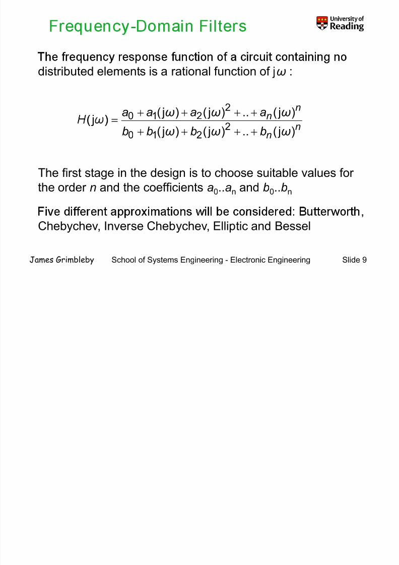
distributed elements is a rational function of jω :

nnaaaa ) j(..) j() j( 2

210 ωωω ++++n

nbbbb ) j(..) j() j( 2210 ωωω ++++

The first stage in the design is to choose suitable values for

the order n and the coefficients a0..an and b0..bn

,

Chebychev, Inverse Chebychev, Elliptic and Bessel




e u erwor approx ma on ga n s max ma y a

-as possible

The gain falls off monotonically in both pass-band (below

= - =

nH

21) j(

ω

ω

+=




(dB)

0-3

g s

log(freq)ω=1 ω= ωs




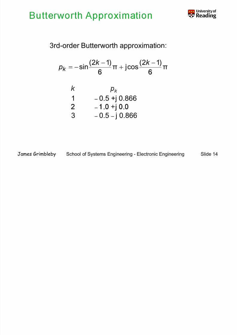
The poles pk of a Butterworth frequency response function

k k k y x p j+=

where:

k k )12()12( −−−

nk

nn

,,2,1

22

K=

Values of k from 1 to n are substituted into this formula

giving the n poles




e po es o e u erwor response p1, p2 , ... , pn are

then combined to give the Butterworth frequency response

) j().. j() j(

) j(

21 n p p p

H

−−−

=ωωω

ω

-

there are no zeros




Poles of H (jω):

– 0.5 + j 0.866 – 0.5 – j 0.866 – 1.0 + j 0.0

Combining the poles:

1) j( =ωH

1

.....

=

+++−+ ωωω

)0.1 j(1.0) j) j((2

+++ ωωω

1.02.0j) j(0.2) j( 23 +++=

ωωω




What order n is required to meet specification?

Gain (dB)

0-

g s

log(freq)ω

=1 ω

=ω




The gain g of a Butterworth filter, expressed in dB, is giveny:

) j(log20 10 H g ω=

og2

-10

n

ω

−=+=

The stop-band edge is at ωs, and the stop-band gain isrequired to be less than g s dB:

sssss

ng

g

ω

ωω

101010

log20

ogog

−≥

−≈+−≥

sg n

−≥




-

( d B )

≥ -3 dB

G a i

g s ≤ -40 dB

ω = 1.0

ωs = 1.5


..



e e yc ev approx ma on ga n osc a es e ween

dB and g p dB in the pass-band (below ω=1)

In the stop-band (above ω=1) the gain falls off

approximation for each n, but a group of approximations

- p

approximation is an all-pole response




(dB)

0g p

g s

log(freq)ω=1 ω= ωs




Res onse of 6th-order Cheb chev a roximation:

(

d B )

g p ≥ -3 dB

G a i n g s ≤ -40 dB

ω p = 1.0

ω

s

= .

Fre uenc Hz 1.00.01School of Systems Engineering - Electronic Engineering Slide 26James Grimbleby



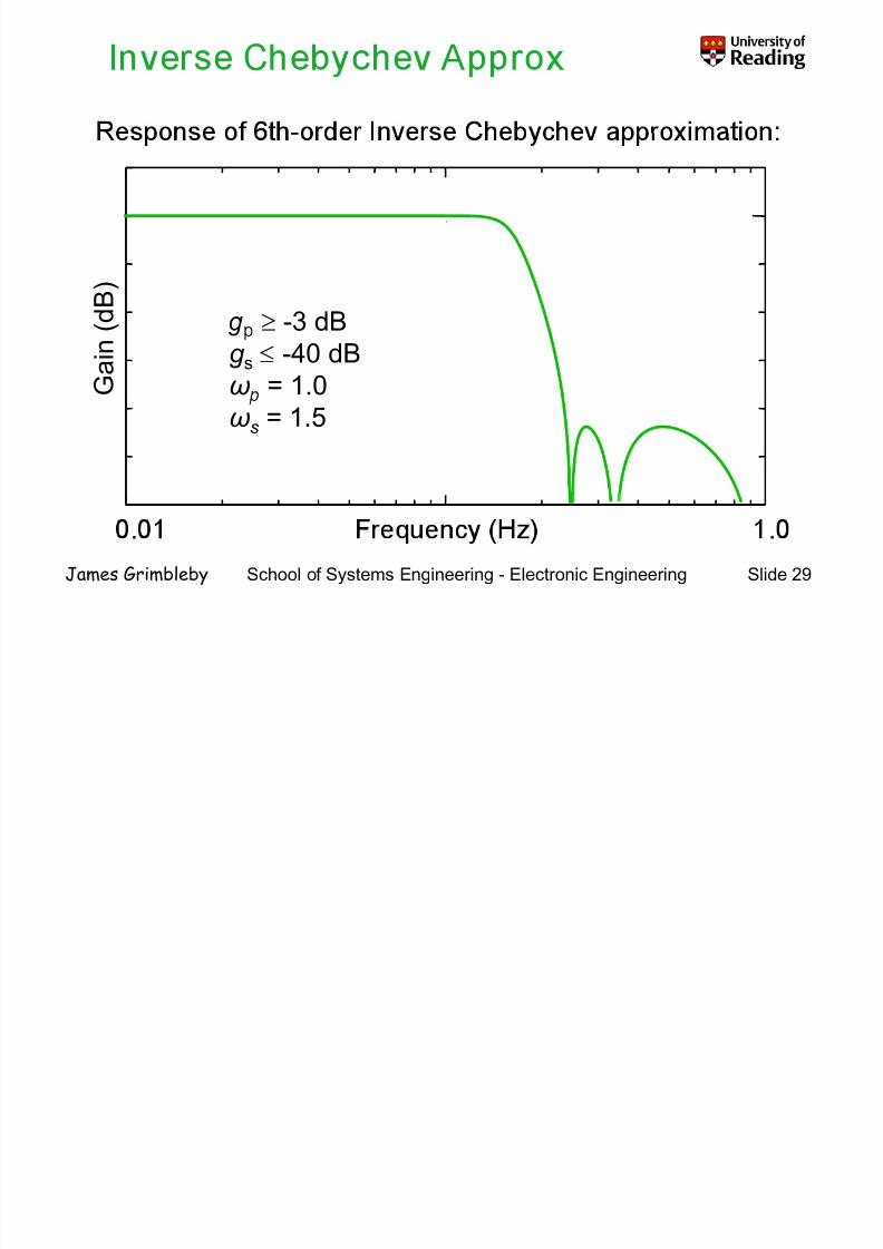
The Inverse Chebychev approximation gain falls off

monotonically in the pass-band (below ω=1)

In the stop-band (above ω=1) the gain at first falls to -∞ dB,

an en osc a es e ween -∞ an g s

approximation for each n, but a group of approximations with

- s




( d B )

≥ -3 dB


ω = 1.0

ωs = 1.5


..



The elliptic response gain oscillates between 0 and g p dB in

-

-

g s dB and -∞ dB

The elliptic approximation has imaginary zeros

For a given filter specification the elliptic approximation givesthe lowest order fre uenc res onse function




a n

(dB)

0g

g s

log(freq)ω=1 ω= ω

s




-

( d B )

≥ -3 dB


ω = 1.0

ωs = 1.5


..



-

- -

1.0

g ( t

0.0


. .



e esse approx ma on s use w ere a requency- oma n

filter is required which also has a good time-domain

-

frequency and the different frequency components are

-

seriously distorted




The Bessel approximation has an all-pole frequencyresponse function:

a0

nnbbbb ) j(..) j() j( 2210 ωωω ++++

n e g - requency m ω→∞:

an

nb ω

≈

00 ba =

)!2( i nb

i ni

−

−=

−




-

d

B )

G a i n


..



- -

.

t ) g (

0.0


. .



- -

TransformationThis transformation shifts the cut-off frequency to ω0:

j jω

ωω →

ω= ω0 ω=1.0




- -

Transformation

Design example: A Chebychev low-pass filter is required with

e o ow ng spec ca on:

ass- an ga n: g p -

Stop-band gain: g s ≤ -50 dB

- p

Stop-band edge: f s = 2000 Hz

This corresponds to a normalised low-pass filter with ωp=1.0,s .




- -

TransformationNormalised low-pass filter:

ass- an ga n: g p ≥ -Stop-band gain: g s ≤ -50 dB

ass- an e ge: ωp= .

Stop-band edge: ωs=2.0

This specification can be met by a 5th-order Chebychev

62650.0=

-

) j(415.1) j(5745.0) j(

2

345 ++ ωωω

School of Systems Engineering - Electronic Engineering Slide 40James Grimbleby...



- -

Transformation Applying the low-pass to low-pass transformation with

ω0=2π×1000=6283:

j j.) j( 345

⎫⎧⎫⎧⎫⎧=

ωωω

ωH

6283.

6283.

6283

2

⎭⎩⎭⎩⎭⎩

06265.06283

4080.06283

5489.0 +⎭⎬

⎩⎨+

⎭⎬

⎩⎨+

ωω

10705.510686.310021.1

62650.0312416519 ×+×+×= −−−

ωωω

06265.0) j(10493.6) j(10390.1 528 +×+×+ −−ωω




- -

Transformation5th-order Chebychev low-pass with cut-off frequency 1000 Hz :

d

B )

a i n




- -

TransformationThis transformation converts to a high-pass response and

shifts the cut-off frequency to ω0:

ωω j 0→

ω= ω0ω=1.0




- -

TransformationDesign example: A Chebychev high-pass filter is required

- p -

Stop-band gain: g s ≤ -25 dB

- =p Stop-band edge: f s = 1000 Hz

This corresponds to a normalised low-pass filter withω =1.0 ω =2.0




- -

TransformationNormalised low-pass filter:

Pass-band gain: g p ≥ -3 dBStop-band gain: g s ≤ -25 dB

Pass-band edge: ωp=1.0

Stop-band edge: ω

s=2.0

This specification can be met by a 3rd-order Chebychev

approx ma on w pass- an r pp e:

2506.0) j(9284.0) j(5972.0) j(

.) j(

23 +++=

ωωω

ωH


- -



- -

Transformation

2506.0) j(9284.0)(5972.0) j(

2506.0) j(

23 +++=

ωωω

ωH

Applying the low-pass to high-pass transformation with

ω0=2π×2000:2506.0

ω =H

2506.012566

9284.012566

5972.012566

ωωω

+⎬⎫

⎨⎧

+⎬⎫

⎨⎧

+⎬⎫

⎨⎧

324712 2506.010167.110431.910984.1

)(2506.0

ωωω

ω

+×+×+×=


- -



- -

Transformation3rd-order Chebychev high-pass with cut-off frequency 2000 Hz :

( d B

G a i


- -



TransformationThis transformation converts to a band-pass response

centred on ω0 with relative bandwidth k 2 :

⎬⎫⎨⎧ +0 jωω

k → 0 jω


0.

- -



Transformation

with relative bandwidth k 2=4:

d

B )

a i n

School of Systems Engineering - Electronic Engineering Slide 49James GrimblebyFrequency (Hz)1000



- -



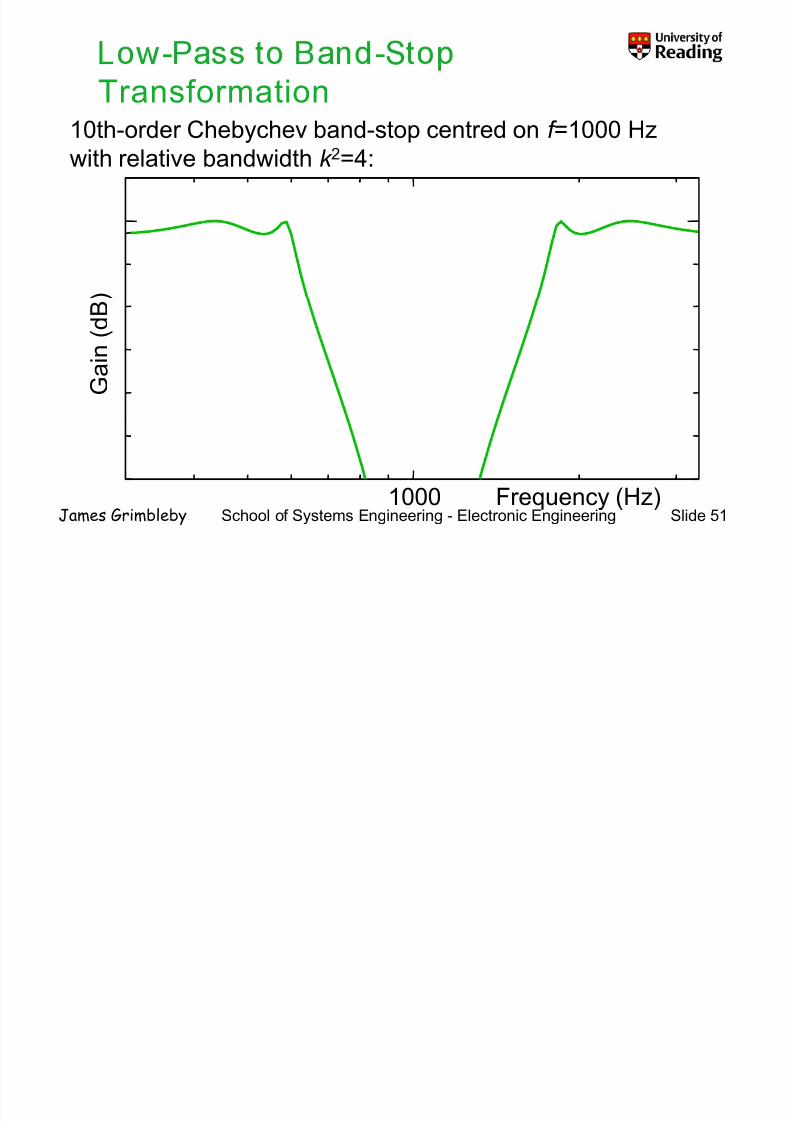
Transformation10th-order Chebychev band-stop centred on f =1000 Hz

with relative bandwidth k 2=4:

)

n ( d B

G

a i

School of Systems Engineering - Electronic Engineering Slide 51James GrimblebyFrequency (Hz)1000



Passive filters are usually realised as equally-terminated

ladder filters

This type of filter has a resistor in series with the input and a

resistor of nominally the same value in parallel with the

output; all other components are reactive (that is inductors orcapacitors)

Passive equally-terminated ladder filters are not normally

used at frequencies below about 10 kHz because they

contain inductors




Equally-terminated low-pass all-pole ladder filter:

R

This type of filter is suitable for implementing all-pole,

=School of Systems Engineering - Electronic Engineering Slide 53James Grimbleby



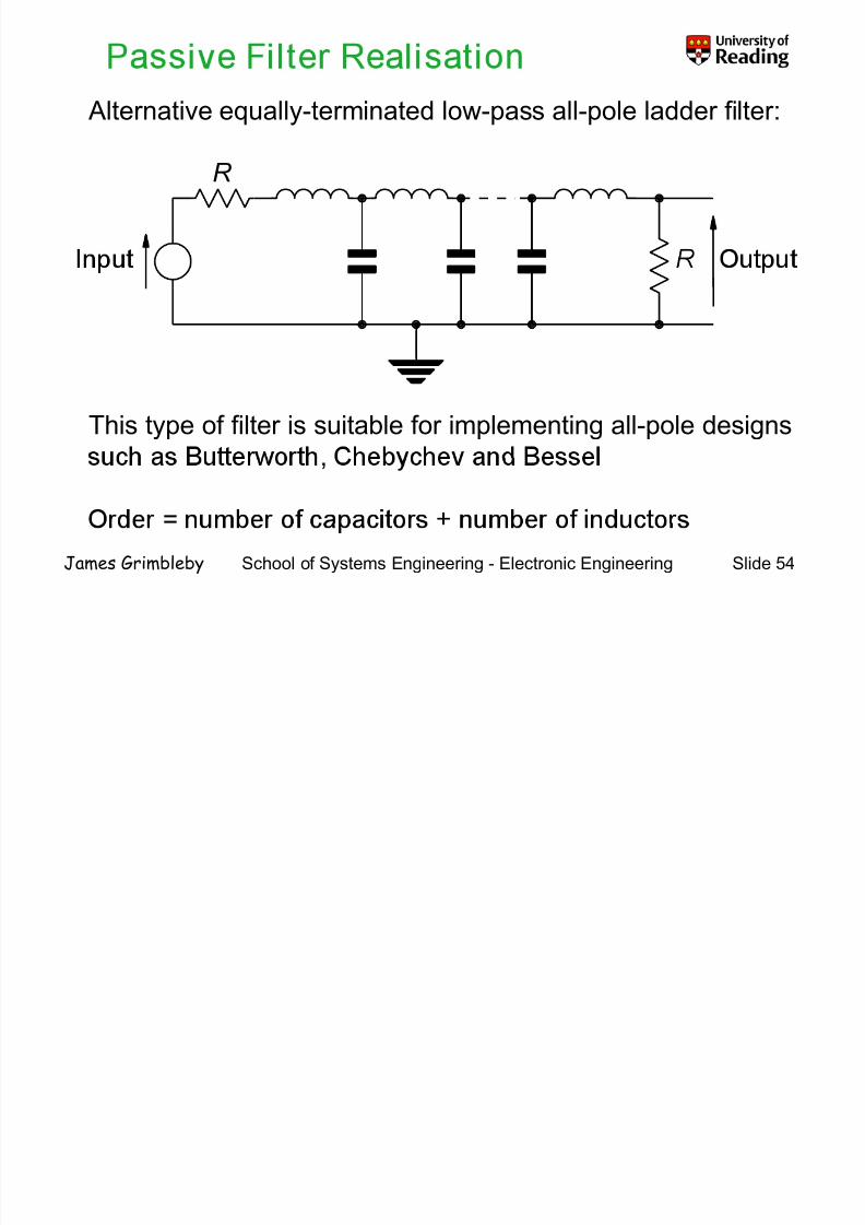
Alternative equally-terminated low-pass all-pole ladder filter:

R

This type of filter is suitable for implementing all-pole designs,

=School of Systems Engineering - Electronic Engineering Slide 54James Grimbleby



- -zeros in response:

R

R Input Output

This type of filter is suitable for implementing an Inverse

Chebychev or Elliptic response




- -imaginary zeros in response:

R Input

Out ut

This type of filter is suitable for implementing an Inverse

Chebychev or Elliptic response




- -replacing the inductors by capacitors, and the capacitors

b inductors:

R

R In ut Out ut

This type of filter is suitable for implementing all-pole

designs such as Butterworth, Chebychev and Bessel




- -

replacing the inductors and capacitors by LC combinations

C L

1=

C

0ω

C LL 1

L2

0ω

=

where ω0 is the geometric centre frequency of the

passband




replacing the inductors and capacitors by LC combinations

R

R Input Output

This type of filter is suitable for implementing all-pole

designs such as Butterworth, Chebychev and Bessel




following procedure:

1. Select a suitable filter circuit

2. Obtain its frequency-response function in symbolic

form

3. Equate coefficients of the symbolic frequency-

response function and the required response

4. Solve the simultaneous non-linear equations to

obtain the component values




-

(R = 1.0 Ω, ω0 = 1.0 rad/s):

n C1 L2 C3 L4 C5 L6 C7

2 1.414 1.4143 1.000 2.000 1.000

4 0.765 1.848 1.848 0.765

5 0.618 1.618 2.000 1.618 0.618

6 0.518 1.414 1.932 1.932 1.414 0.518

7 0.445 1.247 1.802 2.000 1.802 1.247 0.445




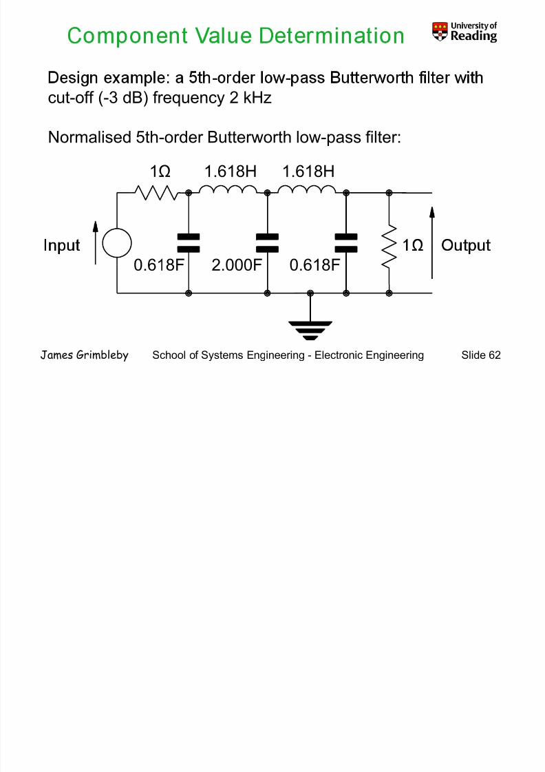
- -cut-off (-3 dB) frequency 2 kHz

Normalised 5th-order Butterworth low-pass filter:

1Ω 1.618H 1.618H

0.618F 0.618F2.000F




k , divide capacitor values by k

Choose k = 10000

10kΩ 10kΩ16.18kH 16.18kH

61.8μF 61.8μF200μF




ca e requency: v e n uc or an capac or va ues y

where k = 2π×2000 = 1.257×104

10kΩ 10kΩ1.288H 1.288H

Input Output

. n . n . n




- -

( d B )

G a i n




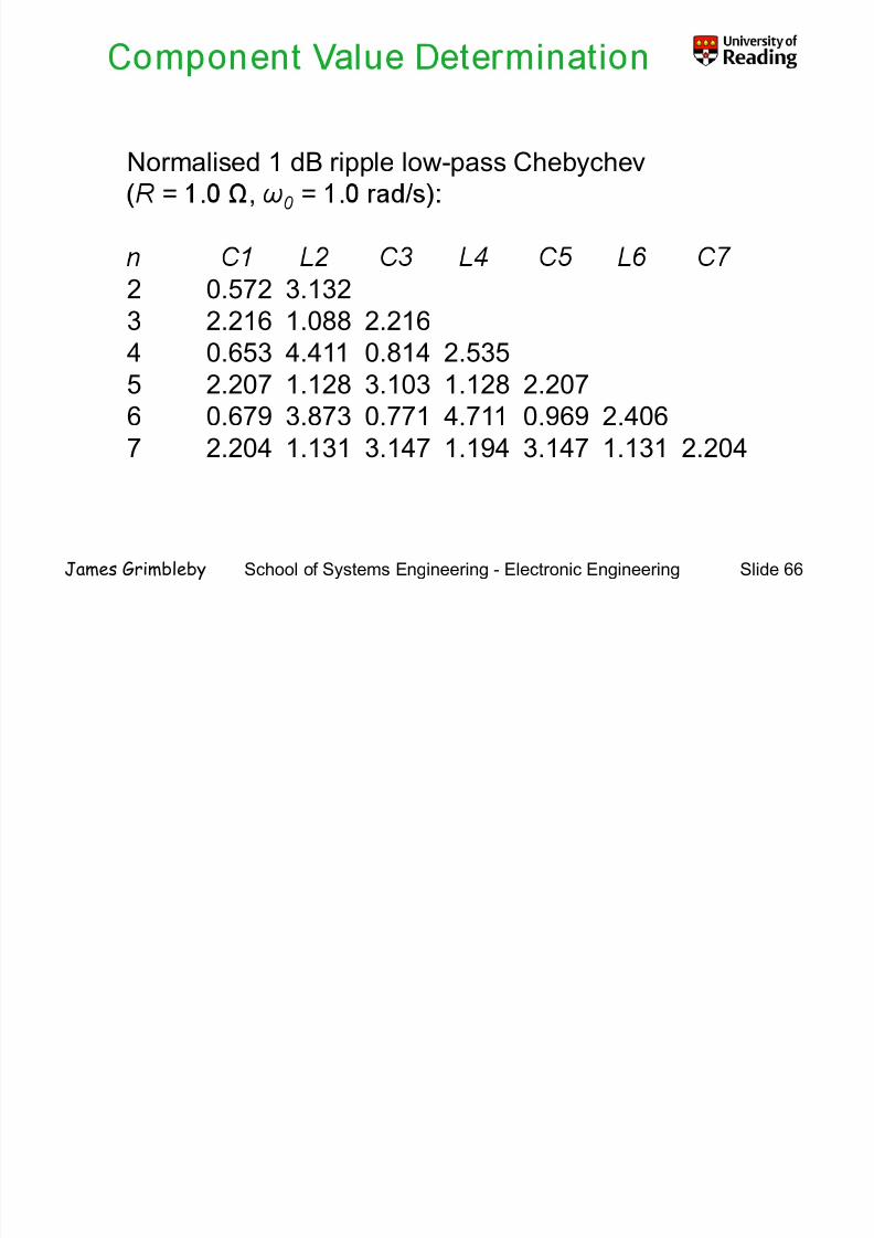
Normalised 1 dB ripple low-pass Chebychev

= =. , .

2 0.572 3.132

3 2.216 1.088 2.2164 0.653 4.411 0.814 2.535

5 2.207 1.128 3.103 1.128 2.207

6 0.679 3.873 0.771 4.711 0.969 2.406

7 2.204 1.131 3.147 1.194 3.147 1.131 2.204




- -1 dB ripple and a cut-off (-3 dB) frequency 5 kHz

Normalised 3rd-order Chebychev high-pass filter:1

1Ω .088.1

1ΩIn ut Out ut0.451H 0.451H

216.2

1




divide capacitor values by k

Choose k = 1000

1000Ω 1000Ω

In ut Out ut451H 451H





where k = 2π×5000 = 3.142×105

1000Ω . 1000Ω

In ut Out ut

14.36mH 14.36mH




- -

( d B )

G a i n




- -1 dB ripple and a cut-off (-3 dB) frequency 5 kHz

Normalised 3rd-order Chebychev high-pass filter:1

.216.2

.

1Ω

1Ω0.919HIn ut Out ut

088.1

1




divide capacitor values by k

Choose k = 1000

919HIn ut Out ut





where k = 2π×5000 = 3.142×105

1000Ω 14.36nF 1000Ω14.36nF

29.25mHInput Output




5th-order 3dB ripple low-pass Chebychev equally-terminated ladder filter with cut-off frequency 1000 Hz:

B )

a i n ( d

±10% variation of

G




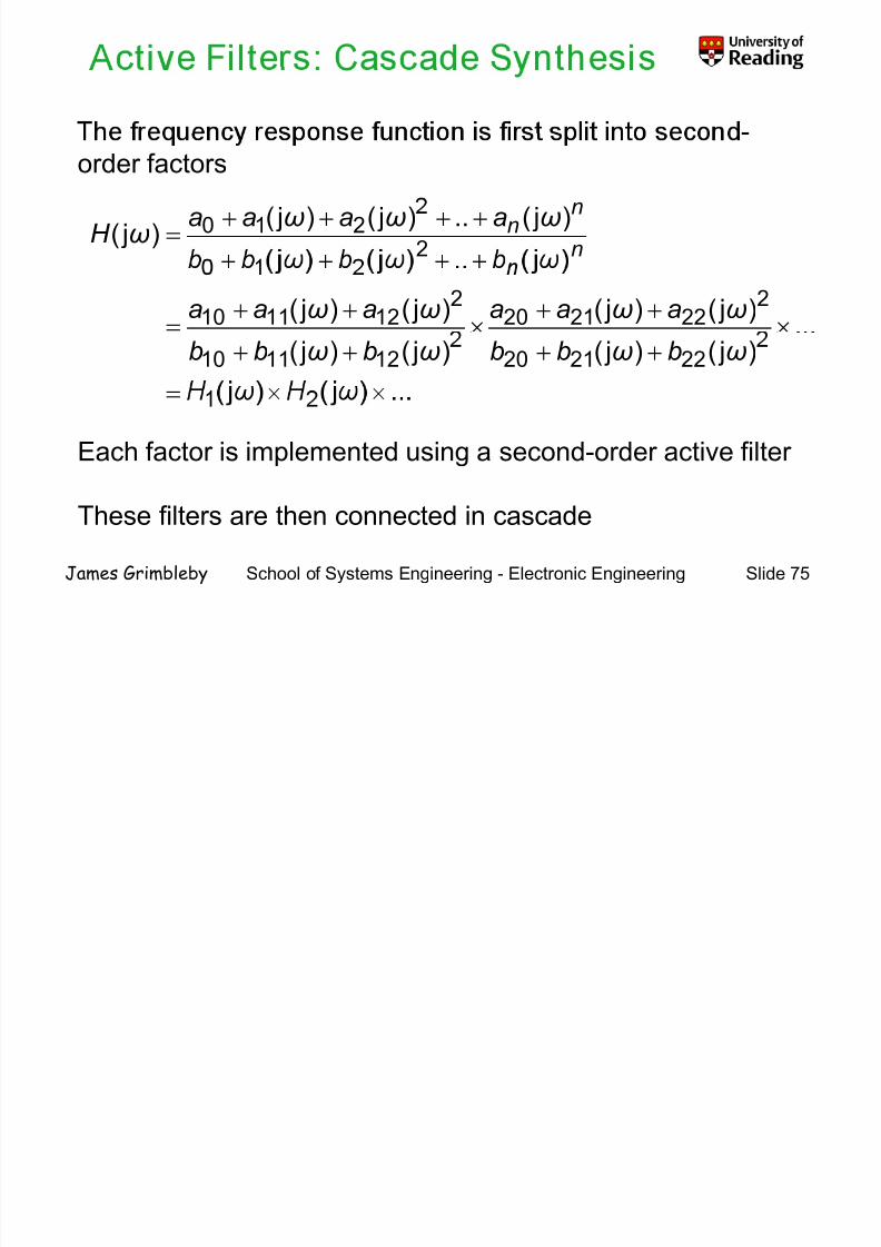
order factors

) j(..) j() j() j( 2210 ++++= ωωω

ω aaaaH n

n

n

) j() j() j() j( 2222120

2121110

×

++

×

++

=

ωωωω aaaaaa

) j() j() j() j( 222120121110

=

++++ ωωωω bbbbbb

Each factor is implemented using a second-order active filter

These filters are then connected in cascade




If the response to be implemented is derived from an all-

pole approximation then the second-order factors will be of

s mp e ow-pass lp , an -pass bp or g -pass hp

form:

2210

0

) j() j() j(

ωω

ω

bbb

aH lp

++=

21 ) j(

) j( ω

ωa

H bp =

22 ) j( ωa2

210 ) j() j( ωω bbb p

++


- -



C 1

R 1 R 2

OutputInputC 2

1) j(H l =ω

22211121

212

:where C R T C R T R R ===

++ ωω


-



2212 ) j() j(21

) j(ωω

ω

T T T H lp

++=Sallen-Key:

Standard response:2

1) j( ω =H lp

200

1ωω

++Q

Thus: 221 211

T T T ==00ω

or:2

1

20210

22 T T Q

T T ===

ω

ω


- -

Gain(dB)



Gain(dB)

20 dB

2=Q 10=Q

0 dB

2

1=Q

-20 dB-

1000 10000 10000010010-40 dB


- -



R

C 1 C 2

u puInputR 2

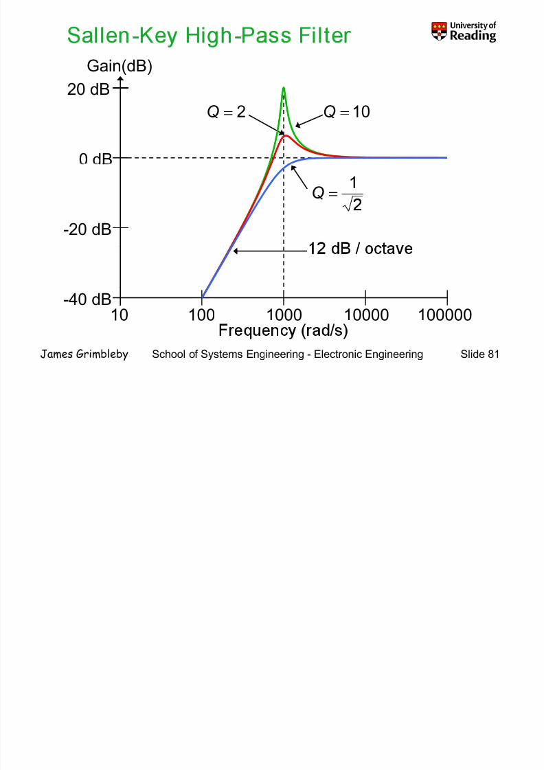
221 ) j() j( T T H = ωω

211

:where

) j() j(21

C R T C R T C C

T T T

===

++ ωω


- -

Gain(dB)



Gain(dB)

20 dB

2=Q 10=Q

0 dB

1=Q

-20 dB

1000 10000 10000010010-40 dB


-



R C 2

R 2 C

1

OutputInput

21 )() j( T H bp −= ω

ω

22211121

212

:where C R T C R T R R ===


-

Gain(dB)



( )

40 dB 10=Q

20 dB 5=Q

2=Q

0 dB

1000 10000 10000010010


-



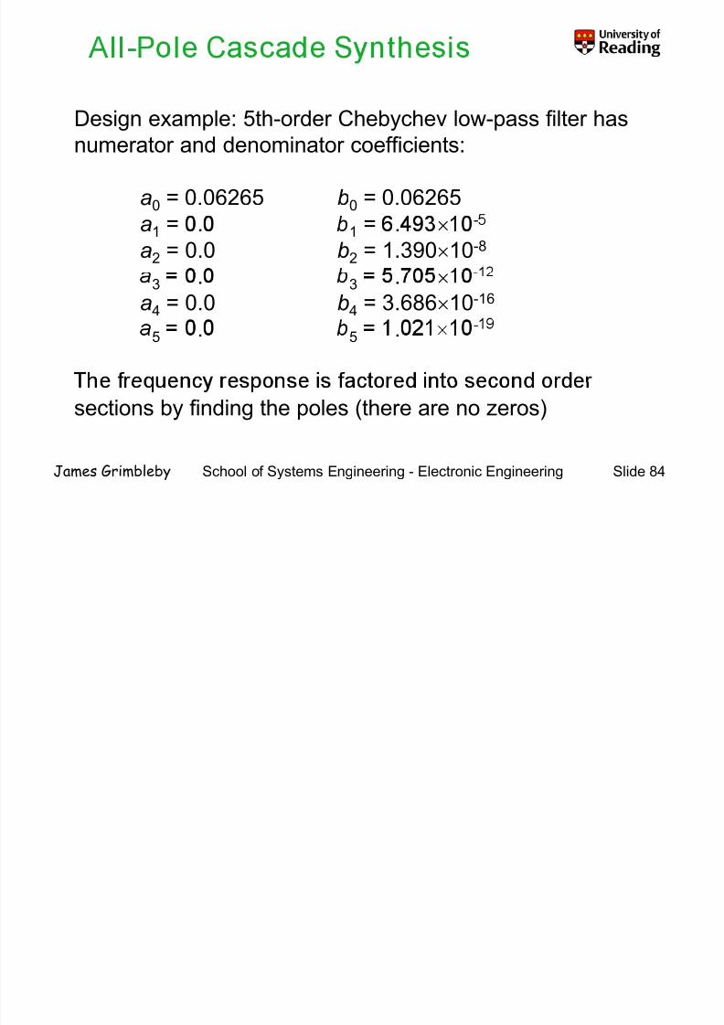
Design example: 5th-order Chebychev low-pass filter has

numerator and denominator coefficients:

a0 = 0.06265 b0 = 0.06265a1 = . 1 = . × -

a2 = 0.0 b2 = 1.390×10-8

-3 . 3 . ×a4 = 0.0 b4 = 3.686×10-16

-5 . 5 .

sections by finding the poles (there are no zeros)


-



The poles are the roots of the equation obtained by setting

the denominator polynomial to zero:

-9.011×10+2 + j3.751×10+3

- . × - . ×-3.463×10+2 + j6.070×10+3

- . × - . ×-1.115×10+3 + j0.0

The frequency response is of 5th-order so that the factors

root


-



Conjugate pole pairs are combined:-9.011×10+2 + j3.751×10+3

+2 +3- . - .

32

32 )10751.3 j109.011(j

..

×+×+

−

ω

2) j(= ω

322

) j)(109.011109.011(

2

×+×+ ω

732 10488.1) j(10802.1) j(

..

++ ×+×+= ωω


-



310115.1 j) j() j( +×+=−= ωωω pD

Dividing through by 1.115×10+3:

Fre uenc res onse function of 1st-order filter:

) j(10966.81) j( ωω −×+=D

1) j( ωH =

Thus: 4×

Let R =10 kΩ; then C =89.66 nF.

. ×


-



Denominator of the 1st 2nd-order section:732 10488.1) j(10802.1) j() j( ++ ×+×+= ωωωD

v ng roug y . × :

284 −−=

Frequency response function of 2nd-order filter:

..

2212 ) j() j(21

) j(ωω

ω

T T T H lp

++=

Thus:

5

2

4

2 10054.610211.12

−−

×=→×= T T

= = = =

121 10110.110718.6 −− ×=→×= T T T


. , .

-



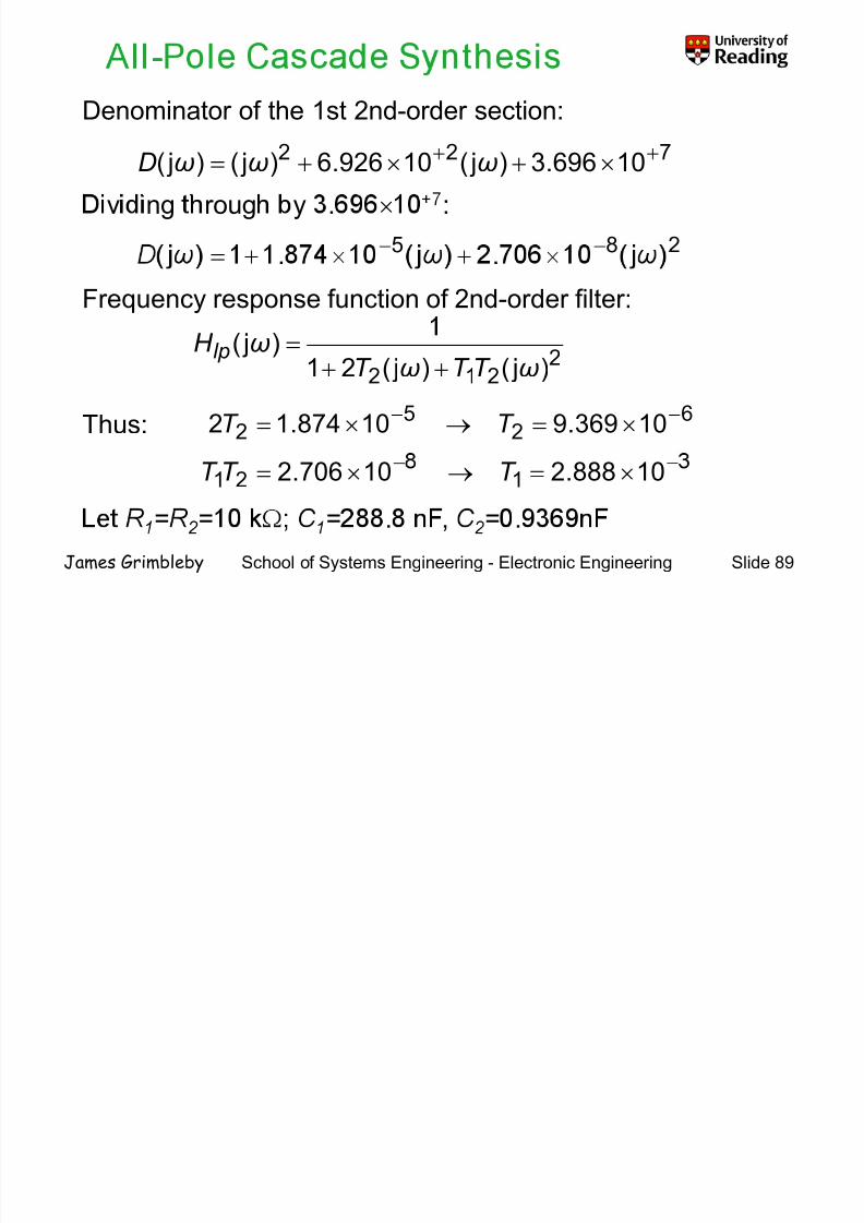
Denominator of the 1st 2nd-order section:722 10696.3) j(10926.6) j() j( ++ ×+×+= ωωωD

v ng roug y . × :

285 −−=

Frequency response function of 2nd-order filter:

..

2212 ) j() j(21

) j(ωω

ω

T T T H lp

++=

Thus:

6

2

5

2 10369.910874.12

−−

×=→×= T T

= = = =

121 10888.210706.2 −− ×=→×= T T T


. , .

-



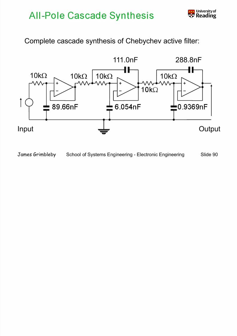
Complete cascade synthesis of Chebychev active filter:

111.0nF 288.8nF

10kΩ 10kΩ 10kΩ 10kΩ

. . .

Input Output




e response s no er ve rom an a -po e approx ma on

then the second-order factors will be of general form:

2210 ) j() j( ωωω

aaaH ++=

210 ) j() j( ωω bbb ++

Rauch or Sallen-Key second-order filters are unsuitable and

- - - -

filter) can be used


5th-order Chebychev low-pass implemented as a cascade



of active Sallen-Key sections:

d B )

a i n




the same low sensitivity properties of passive equally-

passive filter

This is then copied in some way which preserves the

desirable ro erties of the assive filters but which

eliminates the inductors

The copying method that will be described here is based on

inductor simulation




1

3

4131 Z I V V +=3

V 1 322

3231

Z Z V

Z Z V V

++

+=

2 V 210

021

Z Z V V

+=

Z 1

V Z 0


4131 Z I V V +=



41313

22

31Z Z

Z V

Z Z

Z V V

++

+=

021

Z V V =

Substitute to remove V and V :

10

3223321 )( Z V Z V Z Z V +=+

013

123

)(

Z

Z Z Z

V Z V

+

+=

01314112

)()(

Z Z Z V Z I V Z

++−=

School of Systems Engineering - Electronic Engineering Slide 95James Grimbleby0

0



0

−=

)( 30311 Z Z Z Z V ++

Remove cancelling terms:

4201311 Z Z Z I Z Z V =

i

311 Z Z I Z i ==


e an e res s ors o va ue an e a



e 0, 1 , 2,an 4 e res s ors o va ue , an 3 e acapacitor of value C :

23

420 j CR R Z Z Z Z i ω===

or:2

i ==

CR 2

By correct choice of R and C the PIC can be made to

simulate an re uired inductance.


or er e yc ev g pass pass ve er:



-or er e yc ev g -pass pass ve er:

. . .

Input Output4.178H 4.178H 10kΩ

=

F10178.4H178.4 82 ×C CR


5th-order Chebychev high-pass active filter:

9 134 F 9 134 F7 015 F



9.134nF 9.134nF7.015nF10kΩ

10kΩ 10kΩ

u t O

41.78nF41.78nF

I n t p

u t

Ω

Ω10kΩ




395nF382nF

Input Output815nF

1kΩ

2.29H

Let R =1 kΩ; then:62

×


×



high-pass 815nF 395nF382nF1kΩ

1kΩ

2.29μF

Ω

1kΩ1kΩ


sintesis filtros

Documents

Transcript of sintesis filtros