
Sino-German Symposium on Modern Numerical...
33
Sino-German Symposium on Modern Numerical Methods for Compressible Fluid Flows and Related Problems Beijing, May 21-27, 2014 Hyperbolic Techniques for Diffuse Interfaces in Multiphase Flow Christian Rohde Universit¨ at Stuttgart May 23, 2014 1
Transcript of Sino-German Symposium on Modern Numerical...
Sino-German Symposium on
Modern Numerical Methods for Compressible Fluid Flows
and Related Problems
Beijing, May 21-27, 2014
Hyperbolic Techniques for Diffuse Interfaces in Multiphase Flow
Christian RohdeUniversitat Stuttgart
May 23, 2014 1

Plan of the Talk
1) Compressible Navier-Stokes-Korteweg Equations
2) A Hyperbolic Relaxation Approximation
3) The Korteweg/Relaxation Limit
4) Summary and Outlook
Joint work withA. Corli (Ferrara), J. Neusser, V. Schleper (Stuttgart), A. Viorel (Cluj)
May 23, 2014 2
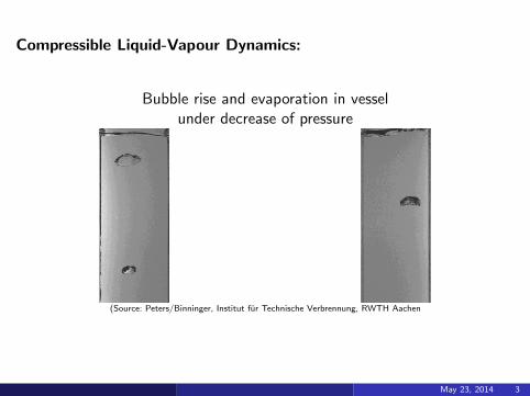
Compressible Liquid-Vapour Dynamics:
Bubble rise and evaporation in vesselunder decrease of pressure
(Source: Peters/Binninger, Institut fur Technische Verbrennung, RWTH Aachen
May 23, 2014 3
1) Compressible Navier-Stokes-Korteweg Equations
(NSK Equations)
May 23, 2014 4
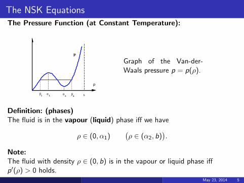
The NSK Equations
The Pressure Function (at Constant Temperature):
ρ
α2 b
α1
β1
β2
p
Graph of the Van-der-Waals pressure p = p(ρ).
Definition: (phases)The fluid is in the vapour (liquid) phase iff we have
ρ ∈ (0, α1)(ρ ∈ (α2, b)
).
Note:The fluid with density ρ ∈ (0, b) is in the vapour or liquid phase iffp′(ρ) > 0 holds.
May 23, 2014 5

The NSK Equations
The Free Energy (at Constant Temperature):
Graph of the free energy W = W (ρ):
p′(ρ) = ρW ′′(ρ).
May 23, 2014 6
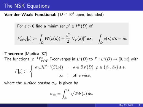
The NSK Equations
Van-der-Waals Functional: (D ⊂ Rd open, bounded)
For ε > 0 find a minimizer ρε ∈ H1(D) of
F εvdW [ρ] :=
∫DW (ρ(x)) +
ε2
2|∇ρ(x)|2 dx,
∫Dρ(x) dx = m.
Theorem: [Modica ’87]The functional ε−1F εvdW Γ-converges in L1(D) to F : L1(D)→ [0,∞] with
F [ρ] :=
{σ∞Hd−1(S(ρ)) : ρ ∈ BV (D), ρ ∈ {β1, β2} a.e.
∞ : otherwise,
where the surface tension σ∞ is given by
σ∞ =
∫ β2
β1
√2W (s) ds.
May 23, 2014 7
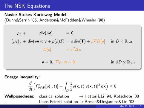
The NSK Equations
Navier-Stokes-Korteweg Model:(Dunn&Serrin ’85, Anderson&McFadden&Wheeler ’98)
ρt + div(ρv) = 0
(ρv)t + div(ρv ⊗ v + p(ρ)I) = ε div(T) + ρ∇D[ρ]
D[ρ] = ε2∆ρ
in D × R>0,
v = 0, ∇ρ · n = 0 in ∂D × R>0
Energy inequality:
d
dt
(F εvdW [ρ(·, t)] +
∫D
1
2ρ(x, t)|v(x, t)|2 dx
)≤ 0
Wellposedness: classical solution → Hattori&Li ’94, Kotschote ’08Lions-Feireisl solution→ Bresch&Desjardins&Lin ’03
May 23, 2014 8
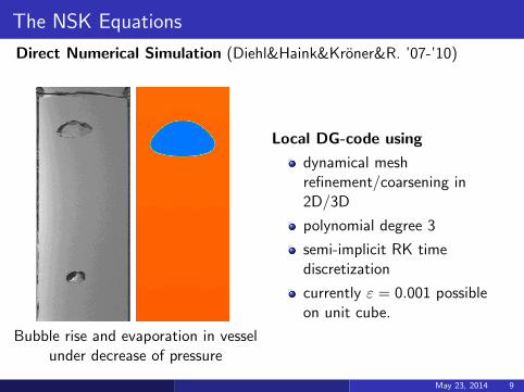
The NSK Equations
Direct Numerical Simulation (Diehl&Haink&Kroner&R. ’07-’10)
Bubble rise and evaporation in vesselunder decrease of pressure
Local DG-code using
dynamical meshrefinement/coarsening in2D/3D
polynomial degree 3
semi-implicit RK timediscretization
currently ε = 0.001 possibleon unit cube.
May 23, 2014 9
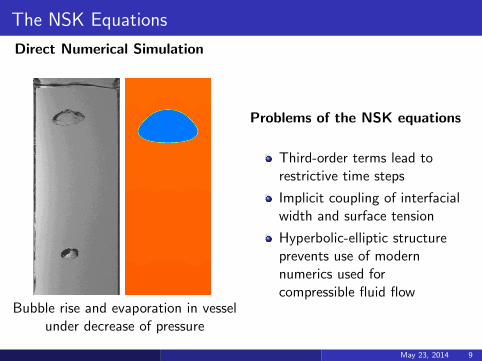
The NSK Equations
Direct Numerical Simulation
Bubble rise and evaporation in vesselunder decrease of pressure
Problems of the NSK equations
Third-order terms lead torestrictive time steps
Implicit coupling of interfacialwidth and surface tension
Hyperbolic-elliptic structureprevents use of modernnumerics used forcompressible fluid flow
May 23, 2014 9
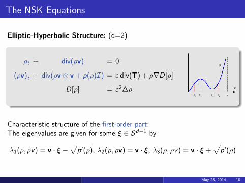
The NSK Equations
Elliptic-Hyperbolic Structure: (d=2)
ρt + div(ρv) = 0
(ρv)t + div(ρv ⊗ v + p(ρ)I) = ε div(T) + ρ∇D[ρ]
D[ρ] = ε2∆ρ ρ
α2 b
α1
β1
β2
p
Characteristic structure of the first-order part:The eigenvalues are given for some ξ ∈ Sd−1 by
λ1(ρ, ρv) = v · ξ −√p′(ρ), λ2(ρ, ρv) = v · ξ, λ3(ρ, ρv) = v · ξ +
√p′(ρ)
May 23, 2014 10
2) A Relaxation Approximation
May 23, 2014 11
Relaxation Approximation
A Relaxed Functional: (Brandon et al.’95, Rogers&Truskinovsky ’97 )
For ε, α > 0 find a minimizer (ρα, cα) ∈ L2(D)× H1(D) of
F ε,αRelax [ρ, c] :=
∫D
(W (ρ) +
α
2(ρ− c)2 +
ε2
2|∇c |2
)dx,
∫Dρ dx = m.
Theorem: [Solci&Vitali ’03]
(i) There is a function σ : (0,∞)→ (0,∞) such that for each α > 0 thefunctional ε−1F ε,αRelax Γ-converges in (L1(D))2 toF : (L1(D))2 → [0,∞] with
F [ρ, c] :=
{σ(α)Hd−1(S(ρ)) : ρ = c ∈ {β1, β2} a.e., ρ, c ∈ BV (D)
∞ : otherwise
(ii) The (surface tension) function σ is monotone increasing and satisfies
limα→∞
σ(α) = σ∞.
May 23, 2014 12
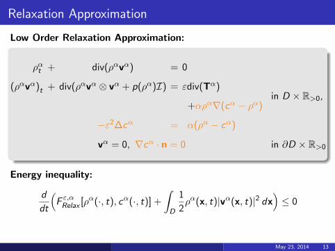
Relaxation Approximation
Low Order Relaxation Approximation:
ραt + div(ραvα) = 0
(ραvα)t + div(ραvα ⊗ vα + p(ρα)I) = εdiv(Tα)
+αρα∇(cα − ρα)
−ε2∆cα = α(ρα − cα)
in D × R>0,
vα = 0, ∇cα · n = 0 in ∂D × R>0
Energy inequality:
d
dt
(F ε,αRelax [ρα(·, t), cα(·, t)] +
∫D
1
2ρα(x, t)|vα(x, t)|2 dx
)≤ 0
May 23, 2014 13
Relaxation Approximation
Low Order Relaxation Approximation:
ραt + div(ραvα) = 0
(ραvα)t + div(ραvα ⊗ vα + p(ρα)I) = εdiv(Tα)
+αρα∇(cα − ρα)
−ε2∆cα = α(ρα − cα)
in D × R>0,
vα = 0, ∇cα · n = 0 in ∂D × R>0
Asymptotic Limits:
(i) Korteweg limit α→∞ towards NSK system
(ii) Sharp-interface limit ε→ 0 towards Euler system
May 23, 2014 13
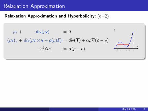
Relaxation Approximation
Relaxation Approximation and Hyperbolicity: (d=2)
ρt + div(ρv) = 0
(ρv)t + div(ρv ⊗ v + p(ρ)I) = div(T) + αρ∇(c − ρ)
−ε2∆c = α(ρ− c)ρ
α2 b
α1
β1
β2
p
May 23, 2014 14

Relaxation Approximation
Relaxation Approximation and Hyperbolicity: (d=2)
ρt + div(ρv) = 0
(ρv)t + div(ρv ⊗ v +
(p(ρ) +
α
2ρ2︸ ︷︷ ︸
=:pα(ρ)
))= εdiv(T) + αρ∇c
−ε2∆c = α(ρ− c)
The new first-order part is strictly hyperbolic for α > max{−W ′′(ρ)}:
λ1(ρ, ρv) = v · ξ −√
p′α(ρ), λ2(ρ, ρv) = v · ξ, λ3(ρ, ρv) = v · ξ +√pα(ρ)
Note: Relaxation approximation has the structure of the shallow-watersystem with bottom topography c .
May 23, 2014 15
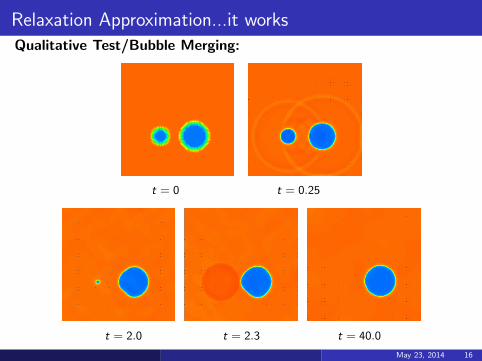
Relaxation Approximation...it works
Qualitative Test/Bubble Merging:
t = 0 t = 0.25
t = 2.0 t = 2.3 t = 40.0
May 23, 2014 16
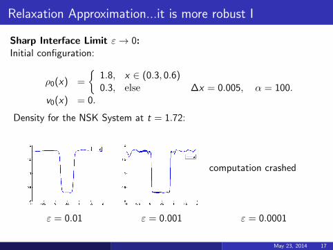
Relaxation Approximation...it is more robust I
Sharp Interface Limit ε→ 0:Initial configuration:
ρ0(x) =
{1.8, x ∈ (0.3, 0.6)0.3, else
v0(x) = 0.∆x = 0.005, α = 100.
Density for the NSK System at t = 1.72:
computation crashed
ε = 0.01 ε = 0.001 ε = 0.0001
May 23, 2014 17

Relaxation Approximation...it is more robust I
Sharp Interface Limit ε→ 0:Initial configuration:
ρ0(x) =
{1.8, x ∈ (0.3, 0.6)0.3, else
v0(x) = 0.α = 100.
Energy evolution for the NSK system with ε = 0.01:
May 23, 2014 17
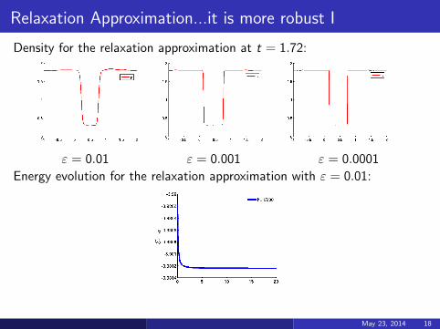
Relaxation Approximation...it is more robust I
Density for the relaxation approximation at t = 1.72:
ε = 0.01 ε = 0.001 ε = 0.0001
Energy evolution for the relaxation approximation with ε = 0.01:
May 23, 2014 18

Relaxation Approximation...it is more robust II
Larger Density Ratio:Initial configuration:
ρ0(x) =
{36, x ∈ (0.3, 0.6)6.0, else
v0(x) = 0.∆x = 0.00025, α = 400, ε = 0.01.
Density evolution for the relaxation approximation:
t = 0.01 t = 0.2 t = 0.5
May 23, 2014 19

Relaxation Approximation
An Energy-Dissipative Discretization:The first-order-part of the relaxation approximation for d = 1:(
ρm := ρv
)t
+ fα
((ρm
))x
= 0⇔ ut + fα(u)x = 0
It is equipped with the entropy/entropy flux pair
ηα(ρ,m) = Wα(ρ) +m2
2ρ, qα(ρ,m) =
m
ρ
(ηα(ρ,m) + pα(ρ)
).
The convexity of ηα implies that the mapping
u 7→ w(u) := ∇ηα(u)
is one-to-one. The relaxation approximation can be rewritten in the form
u(w)t + gα(w)x = 0.
May 23, 2014 20

Relaxation Approximation
Theorem (Tadmor ’84, ’03)For the relaxation approximation there is a 2-parameter family ofnumerical fluxes g∗ = g∗(w, z) such that the scheme
u′j(t) = − 1
∆x
(g∗j+ 1
2(t)− g∗
j− 12(t)), g∗
j+ 12(t) = g∗(wj(t),wj+1(t)),
is entropy-conservative, i.e. there is a numerical entropy flux q∗ = q∗(w, z)that satisfies q∗(w,w) = qα(w) with
ηα(uj(t))′ = − 1
∆x
(q∗j+ 1
2(t)− q∗
j− 12(t))
for all t ∈ (0,T ) and j ∈ Z.
May 23, 2014 21

Relaxation Approximation
Theorem: (Neusser&R.’14)There exists at least one Tadmor flux g∗ = g∗(w, z) such that for
h∗(w, z) =
g∗
1 (w,z)w2
: w2 6= 0,
W ′−1α
(w1 + w2
2
): w2 = 0.
the solution of
u′ +1
∆x
(g∗j+ 1
2− g∗
j− 12
)=
α
∆x
(0
h∗(wj ,wj−1)(cj+1 − cj
)),
ε2
∆x2(cj+1 − 2cj + cj−1) = α(cj − ρj)
satisfies the energy equality
d
dt
∑j∈Z
(m2
j
2ρj+ W (ρj) +
α
2(ρj − cj)
2 +ε2
2∆x2(cj+1 − cj)
2
)= 0.
May 23, 2014 22
3) Analysis of the Korteweg Limit
May 23, 2014 23

Korteweg Limit
A Numerical Example: Let d = 1, ε = 0.01, and ∆x = 0.00125
ρ0(x) =
{1.8 : x ∈ (0.3, 0.6) ∪ (0.85, 1.05)0.3 : else
, v0(x) = 0
Evolution for relaxation approximation uα∆x
t = 0.02 t = 0.04 t = 4
Numerical convergence towards NSK solution u∆x
α 1 5 10 100 1000
‖uα∆x − u∆x‖L2 1.039e-1 3.333e-2 1.802e-2 1.909e-3 1.683e-4
EOC - 0.708 0.885 0.975 1.055
May 23, 2014 24
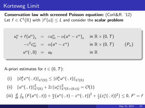
Korteweg Limit
Conservation law with screened Poisson equation: (Corli&R. ’12)Let f ∈ C 1(R) with |f ′(u)| ≤ L and consider the scalar problem
uαt + f (uα)x = εuαxx − α(uα − cα)x in R× (0,T )
−ε2cαxx = α(uα − cα) in R× (0,T )
uα(·, 0) = u0 in R
(Pα)
A-priori estimates for t ∈ (0,T ):
(i) ‖∂kx cα(·, t)‖L2(R) ≤ ‖∂kx uα(·, t)‖L2(R)
(ii) ‖uα(., t)‖2L2(R) + 2ε‖uαx ‖
2L2(R×(0,t)) = O(1)
(iii) ddt
∫R(F (uα(·, t)) + α
2 (uα(·, t)− cα(·, t))2 + ε2 (cαx (·, t))2
)≤ 0, F ′ = f
May 23, 2014 25
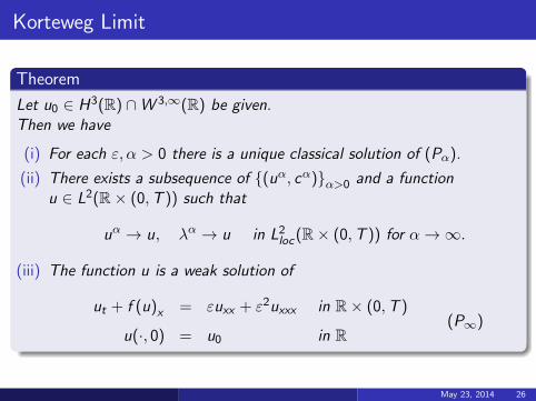
Korteweg Limit
Theorem
Let u0 ∈ H3(R) ∩W 3,∞(R) be given.Then we have
(i) For each ε, α > 0 there is a unique classical solution of (Pα).
(ii) There exists a subsequence of {(uα, cα)}α>0 and a functionu ∈ L2(R× (0,T )) such that
uα → u, λα → u in L2loc(R× (0,T )) for α→∞.
(iii) The function u is a weak solution of
ut + f (u)x = εuxx + ε2uxxx in R× (0,T )
u(·, 0) = u0 in R(P∞)
May 23, 2014 26
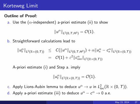
Korteweg Limit
Outline of Proof:
a. Use the (α-independent) a-priori estimate (ii) to show
‖uα‖L2(0,T ;H3) = O(1).
b. Straightforward calculations lead to
‖uαt ‖L2(R×(0,T )) ≤ C (‖uα‖L2(0,T ;H2)) + α‖uαx − cαx ‖L2(R×(0,T ))
= O(1) + ε2‖cαxxx‖L2(R×(0,T ))
A-priori estimate (i) and Step a. imply
‖uαt ‖L2(R×(0,T )) = O(1).
c. Apply Lions-Aubin lemma to deduce uα → u in L2loc(R× (0,T )).
d. Apply a-priori estimate (iii) to deduce uα − cα → 0 a.e.
May 23, 2014 27

Korteweg Limit
Extensions of the Analysis:
Conservation law with screened heat equation (Corli&R.&Schleper ’14)
uαt + f (uα)x = εuαxx − α(uα − cα)xεαc
αt − ε2cαxx = α(uα − cα)
NSK system in Lagrangean coordinates (R.&Viorel ’14)
ταt − vαx = 0vαt + p(τα)x = εvαxx − α(τα − cα)x
ε2cαxx = α(uα − cα)
Note: Korteweg limit for NSK systems in Charve ’13 and Giesselmann ’14.
May 23, 2014 28
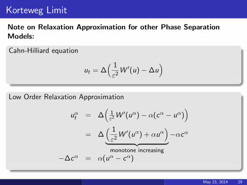
Korteweg Limit
Note on Relaxation Approximation for other Phase SeparationModels:
Cahn-Hilliard equation
ut = ∆( 1
ε2W ′(u)−∆u
)
Low Order Relaxation Approximation
uαt = ∆(
1ε2W
′(uα)− α(cα − uα))
= ∆( 1
ε2W ′(uα) + αuα
)︸ ︷︷ ︸monotone increasing
−αcα
−∆cα = α(uα − cα)
May 23, 2014 29
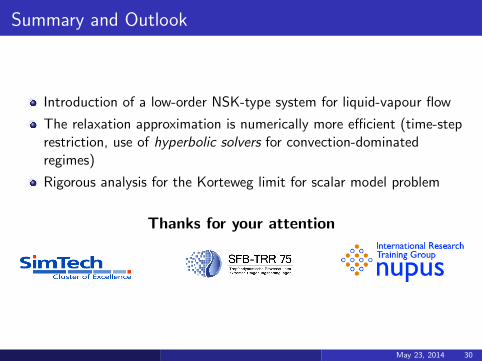
Summary and Outlook
Introduction of a low-order NSK-type system for liquid-vapour flow
The relaxation approximation is numerically more efficient (time-steprestriction, use of hyperbolic solvers for convection-dominatedregimes)
Rigorous analysis for the Korteweg limit for scalar model problem
Thanks for your attention
May 23, 2014 30