Singular sources mining using evidential conflict analysis

International Journal of Approximate Reasoning 52 (2011) 1433–1451

Contents lists available at SciVerse ScienceDirect

International Journal of Approximate Reasoning

j o u r n a l h o m e p a g e : w w w . e l s e v i e r . c o m / l o c a t e / i j a r

Singular sources mining using evidential conflict analysis

John Klein ∗, Olivier ColotLAGIS – FRE CNRS 3303, University of Lille1, France

A R T I C L E I N F O A B S T R A C T

Article history:

Received 27 January 2011

Received in revised form 10 August 2011

Accepted 12 August 2011

Available online 25 August 2011

Keywords:

Dempster–Shafer theory

Conflict analysis

Outlier detection

Singular sourcesmining is essential inmany applications like sensor fusion or dataset analy-

sis. A singular source of information provides pieces of evidence that are significantly dif-

ferent from the majority of the other sources. In the Dempster–Shafer theory, the pieces of

evidence collected by a source are summarized by basic belief assignments (bbas). In this

article, we propose to mine singular sources by analyzing the conflict between their corre-

sponding bbas. By viewing the conflict as a function of parameters called discounting rates,

new developments are obtained and a criterion that weights the contribution of each bba to

the conflict is introduced. The efficiency and the robustness of this criterion is demonstrated

on several sets of bbas with various specificities.

© 2011 Elsevier Inc. All rights reserved.

1. Introduction

The Belief Function Theory (BFT), also known as the Dempster–Shafer theory [1,2], has gained popularity because it can

process data that are not only uncertain but also imprecise and then aggregate these different data using a combination

rule. When tackling data fusion problem, a major difficulty to resolve is how to deal with conflicting pieces of information.

The BFT allows the computation of a measure called the degree of conflict. This measure is an indication on how much the

sources of information, from which data are originated, are in conflict. Smets [3] analyzed combination processes in case of

conflicting sources i.e. when the degree of conflict is positive. Yet the degree of conflict has a major drawback in the sense

that it does not evaluate how each source individually contributes to the conflict.

A more refined analysis of conflicting pieces of evidence can indeed bring valuable information as it allows to outline

that some data appears to be singular as compared to the whole data collection. Singularity ranges from a situation where

a piece of evidence is completely isolated to a situation where a piece of evidence shares common view with a substantial

proportion of the collected pieces. It is thus a notion that needs to be gradually evaluated in order to be efficiently integrated

inside an information processing system.

Individual evaluations of the singularity of pieces of evidence are notably of great importance in the field of outlier,

fault or novelty detection. Hodge and Austin [4] propose an extensive survey of outlier detection methodologies. The safety

performances at stake are presented and a broad range of approaches are analyzed amongwhich statistical methods, neural

networks andmachine learningare found. There are ties betweenconflicting andoutlyingdata andwebelieve that thedegree

of conflict encompasses precious information toward the identification of singular or outlying data, hence the motivation to

investigate on new conflict analysis criteria.

Martin et al. [5] and Schubert [6,7] have both proposed criteria that allow an individual measure of conflict for each bba

involved into a combination process. However both of these approaches are highly dependent on the proportion of singular

bbas and the total number of processed bbas.

These dependencies make them difficult to use in contexts where these two quantities may vary. We propose in this

article a new criterion that is more robust to the variations of the proportion of conflicting bbas as well as to the number

∗ Corresponding author.

E-mail addresses: [email protected] (J. Klein), [email protected] (O. Colot).

0888-613X/$ - see front matter © 2011 Elsevier Inc. All rights reserved.

doi:10.1016/j.ijar.2011.08.005

http://dx.doi.org/10.1016/j.ijar.2011.08.005

http://www.sciencedirect.com/science/journal/0888613X

www.elsevier.com/locate/ijar

http://dx.doi.org/10.1016/j.ijar.2011.08.005

1434 J. Klein, O. Colot / International Journal of Approximate Reasoning 52 (2011) 1433–1451

of bbas. This criterion is derived by analyzing the degree of conflict as a function of discounting rates. Discounting rates are

used as part of a belief updating mechanism. A bba yielded by a source that is known to be unreliable is assigned a large

discounting rate so that its weight in the combination process is reduced.

In this paper Section 1 presents general facts about belief functions and the BFT. Section 2 contains an overview of

conflicting bba characterization methods. Our new criterion is presented and justified. Section 3 presents experiments on

synthetic sets of bbas. These sets are mainly made of simple support bbas so as to highlight the differences between the

proposed criterion and existing criteria.

2. Dempster–Shafer theory: fundamental concepts

2.1. Problem modeling

The BFT provides a formal framework for dealing with both imprecise and uncertain data. The finite set of mutually

exclusive solutions is denoted by Ω = {ω1, . . . , ωK} and is called the frame of discernment. The set of all subsets of Ω is

denoted by 2Ω . A source Si collects pieces of evidence leading to the assignment of belief masses to some elements of 2Ω .

The mass of belief assigned to A by Si is denotedmi (A). The functionmi is called basic belief assignment (bba) and is such

that:

mi : 2Ω → [0, 1] (1)∑A⊆Ω

mi (A) = 1 (2)

The set of all bbas is denoted by BΩ .

A set A such that mi (A) > 0 is called a focal element of mi. Two elements of 2Ω represents hypotheses with noteworthy

interpretations:

• ∅: the solution of the problem may not lie within Ω .• Ω: the problem’s solution lies in Ω but is undetermined.

Considering the interpretation of ∅, two assumptions can be made concerning the frame of discernment. The open-world

assumption states that m (∅) > 0 is possible. The closed-world assumption bans ∅ from any belief assignment.

A bba is denoted by Amx if it has two focal elements: Ω and A � Ω , and if:

Amx (A) = 1− x and Amx (Ω) = x (3)

with x ∈ [0, 1]. Such bbas are called simple bbas (sbbas). By extension of this notation, the bba denoted by Am0, or simplyAm, stands for the certainty that the truth belongs to A. Thus, Ωm stands for total ignorance (Ωm(Ω) = 1); it is called the

vacuous bba. This set of bbas are called categorical bbas.

Furthermore, a bba such that m (Ω) = 0 is said to be dogmatic. It is said to be normalized if m (∅) = 0.

2.2. Pieces of evidence combination

Suppose one has obtained two bbas from two distinct 1 pieces of evidence Ev1 and Ev2 collected respectively by sources

S1 and S2. Let us further imagine that Ev2 states that the solution of the problem lies for sure in a set A ⊂ Ω . This piece of

information is thus represented by the bba m2 = Am.

Thebasic combinationproblemconsists infinding away to aggregatem1 andAm. In thebayesian framework, this situation

is known as conditioning and it is named likewise in the BFT. To integrate the information represented by Am into m1, an

intuitive solution is to reassign any mass allocated to a focal element B ofm1 to the intersection of A and B. This leads to the

following formula :

m1 [A] (X) = ∑B|B∩A=X

m1 (B) (4)

with m1 [A] the bba m1 conditioned on A. Now, one can generalize this process to define a combination rule between any

bbas m1 andm2. This leads to the definition of the most commonly used combination rule in the BFT : the conjunctive rule∩© :

∀X ∈ 2Ω, m1 ∩©2 (X) = ∑B,C|B∩C=X

m1 (B)m2 (C) (5)

1 Pieces of evidence are distinct if the construction of beliefs according to one piece of evidence does not restrict the construction of beliefs using another piece

of evidence.

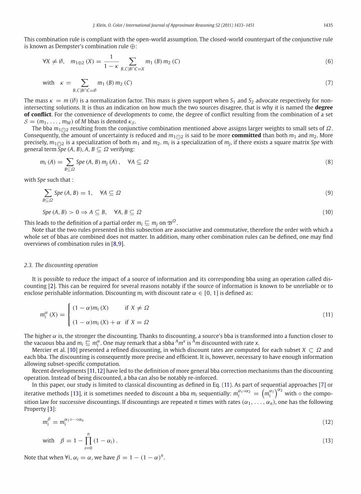
J. Klein, O. Colot / International Journal of Approximate Reasoning 52 (2011) 1433–1451 1435

This combination rule is compliant with the open-world assumption. The closed-world counterpart of the conjunctive rule

is known as Dempster’s combination rule⊕:

∀X �= ∅, m1⊕2 (X) = 1

1− κ

∑B,C|B∩C=X

m1 (B)m2 (C) (6)

with κ = ∑B,C|B∩C=∅

m1 (B)m2 (C) (7)

The mass κ = m (∅) is a normalization factor. This mass is given support when S1 and S2 advocate respectively for non-

intersecting solutions. It is thus an indication on how much the two sources disagree, that is why it is named the degree

of conflict. For the convenience of developments to come, the degree of conflict resulting from the combination of a set

S = (m1, . . . ,mM) of M bbas is denoted κS .The bba m1 ∩©2 resulting from the conjunctive combination mentioned above assigns larger weights to small sets of Ω .

Consequently, the amount of uncertainty is reduced and m1 ∩©2 is said to be more committed than both m1 and m2. More

precisely, m1 ∩©2 is a specialization of both m1 and m2. mi is a specialization of mj , if there exists a square matrix Spe with

general term Spe (A, B), A, B ⊆ Ω verifying:

mi (A) =∑B⊆Ω

Spe (A, B)mj (A) , ∀A ⊆ Ω (8)

with Spe such that :∑B⊆Ω

Spe (A, B) = 1, ∀A ⊆ Ω (9)

Spe (A, B) > 0⇒ A ⊆ B, ∀A, B ⊆ Ω (10)

This leads to the definition of a partial order mi mj on BΩ .

Note that the two rules presented in this subsection are associative and commutative, therefore the order with which a

whole set of bbas are combined does not matter. In addition, many other combination rules can be defined, one may find

overviews of combination rules in [8,9].

2.3. The discounting operation

It is possible to reduce the impact of a source of information and its corresponding bba using an operation called dis-

counting [2]. This can be required for several reasons notably if the source of information is known to be unreliable or to

enclose perishable information. Discounting mi with discount rate α ∈ [0, 1] is defined as:

mαi (X) =

⎧⎪⎨⎪⎩

(1− α)mi (X) if X �= Ω

(1− α)mi (X)+ α if X = Ω

(11)

The higher α is, the stronger the discounting. Thanks to discounting, a source’s bba is transformed into a function closer to

the vacuous bba and mi mαi . One may remark that a sbba Amx is Am discounted with rate x.

Mercier et al. [10] presented a refined discounting, in which discount rates are computed for each subset X ⊂ Ω and

each bba. The discounting is consequently more precise and efficient. It is, however, necessary to have enough information

allowing subset-specific computation.

Recent developments [11,12] have led to the definition of more general bba correctionmechanisms than the discounting

operation. Instead of being discounted, a bba can also be notably re-inforced.

In this paper, our study is limited to classical discounting as defined in Eq. (11). As part of sequential approaches [7] or

iterative methods [13], it is sometimes needed to discount a bba mi sequentially: mα1◦α2

i =(m

α1

i

)α2with ◦ the compo-

sition law for successive discountings. If discountings are repeated n times with rates (α1, . . . , αn), one has the following

Property [3]:

mβi = m

α1◦···◦αn

i (12)

with β = 1−n∏

i=0(1− αi) . (13)

Note that when ∀i, αi = α, we have β = 1− (1− α)n.


3. Singular bbas mining using the degree of conflict

3.1. Problem statement and related works

Aclassical tricky situationwithwhichdata fusion systemdevelopershave todealwith is to combinea set of sources among

which some conflicting sources are found. As experienced by these developers, the conflict observed does not originate from

conflicting sources in identical proportions. In particular, singular sources prevail in conflict generation. By singular, one

may understand a source that delivers information that is significantly different from the rest of the sources. Being singular

or not is thus dependent on the fact that a source is in accordance with the majority opinion or not.

The difficulty is that a source can either be singular or outlying:

• because the device or the agent from which information is derived are respectively faulty or unreliable,• because this source has detected some evidence to which other sources are blind, and this source is consequently

very informative.

In the first case, singular sources must be detected and treated as erroneous to make the fusion process more robust. In the

second case, singular sources must be identified and trigger an ad hoc process so that the information it contains is not lost

or under-weighted as compared to the majority opinion.

In theBFT, each source Si yields a bbami and consequently, singular sourcemining and singular bbamining areunderstood

in the same way in the rest of the paper. BFT approaches for outlier detection are proposed in [14,15] but they do not use

BFT tools for the outlier detection itself. The BFT is used to aggregate pieces of evidence on the presence of an outlier or

not. Instead, we propose here to investigate how the singularity of some evidence can be pinpointed by the BFT. Indeed,

combining a set S = (m1, . . . ,mM) ofM bbas derived from singular sources will always result in a positive value for κ . Thegreater the discordance is, and the larger the number of singular sources are, the higher κ will be. Some criteria related to

the degree of conflict can consequently be defined so as to detect singular bbas but a more detailed analysis than a single

valued measure is needed.

First, multiple bba-dependent values are needed in order to obtain an evaluation of the contribution of each bba to the

conflict. Second, for each bba this value must represent its singularity as compared to the values assigned to the other bbas.

There are many ways to obtain a criterion of this kind. Defining new criteria is a task that requires specifications before

starting to design such a mathematical tool. As part of such specifications, formal properties need to be defined. Properties

are a simple and clear way of stating the goal that we intend to reach.

As reasoning in the general case is not an easy task in the BFT, let us focus on a specific situation that is easy to interpret

and analyze. Suppose one has to process the following bba set Sspe: Sspe = s1 ∪ s2 and ∀m ∈ s1, m = Amx , ∀m ∈ s2,

m = Bmx with A∩B = ∅. Let us denoteM = ∣∣Sspe

∣∣ (with |X| the cardinal of set X) and ri = |si||S| . r1 represents the proportionof bbas belonging to s1 and if |s1| < |s2| these bbas are singular as compared to those belonging to s2 which correspond to

the majority group. All bbas are identically committed in this example therefore the conflict contribution value assigned to

a bba should be a simple expression of r1 or r2. We thus propose the definition of the following homogeneity property:

Property 1. Let Sspe be a bba set defined as above and γi the value assigned to mi and representing its contribution to the conflict.

The criterionγ is homogeneous if,∀i ∈ {1, . . . ,M} and j ∈ {1, 2}, whenmi ∈ sj, we haveγi = h(rj)with h :]0, 1] → [0,+∞)

a bijective decreasing function independent of M with h (1) = 0.

The function h has to be decreasing because a gradual evaluation of the singularity is needed: the larger the proportion

of bbas belonging to a group is, the smaller its contribution to the conflict is. Note that when one has r1 = r2 = 0.5, then a

homogeneous criterion assigns the same value to all bbas. It is also desirable for h to be bijective so that one can fully control

the criterion on this simple specific situation: one proportion of singular bbas is associated to one value and conversely.

Finally, h is also independent ofM because the same proportion of singular bbas implies the same contribution to the conflict

whether the bba set is large or not.

Recently, Schubert [6,7] proposed a criterion ci, called the degree of falsity, that identifies to some extent the contribution

of each individual bba mi involved in the computation of κS :

ci = κS − κS\{mi}1− κS\{mi}

(14)

where S \ {mi} is the set difference of S and {mi}. It is clear that if mi is the only bba advocating for a particular solution,

there will be a huge drop from κS to κS\{mi}. Consequently, this very singular bba will have a large degree of falsity.

This criterion can be addressed a criticism because if there are at least two singular bbas in S , the drop will be far less

large. Looking at the specific situation depicted by the set Sspe, the degree of falsity is very efficient but when r > 1/M,

the detection of singular bbas may be impaired. ci is obviously non-linear with respect to r and these non-linearities are

dependent on the total numberM of bbas involved in the fusionprocess. Thedegree of falsity fails to possess thehomogeneity

property and cannot be fully controlled on such a simple set as Sspe.


Anotherminor drawback of ci is alsometwhen categorical bbas are aggregated. Onemaywell have κS\{mi} = 1, meaning

that removingmi does not suffice to avoid the full conflict case. In this situation, the falsity criterion reaches an undetermined

value. In this paper, we consider that this value is 0 since it is not possible to conclude on the falsity ofmi. It may be possible

to introduce a parameter to prevent bbas from being categorical, but this implies an additional parameter tuning.

Martin et al. [5] have also introduced several criteria, called conflict measures, evaluating the conflict provoked by a

bba as compared to a set of bbas. These criteria are defined using a distance dBPA between bbas introduced by Jousselme

et al. [16]:

dBPA (m1,m2) =√1/2 ( �m1 − �m2)

tD ( �m1 − �m2) (15)

with �m a vector form2 of the bba m and D a 2N × 2N matrix whose elements are D (A, B) = |A ∩ B| / |A ∪ B|. Martin et al.

propose then the following conflict measures Confi :

Confi = 1

M − 1

M∑j=1,i �=j

dBPA(mi,mj

)(16)

or Confi = dBPA (mi,m∗) (17)

with m∗ the combination of bbas in S \ {mi}. m∗ can be obtained using different combination rules or by using the mean.

Furthermore, the authors propose to tune this measure using a function f :

f (Confi) (18)

The heuristic choice for f indicated by the authors is f (x) = 1−(1− xλ

)1/λand λ = 1.5.

For some of the conflictmeasures, it can be shown that a bijective decreasing function h can be foundwhen one processes

a bba set such as Sspe. However, these functions fail to be independent of M and consequently conflict measures are not

homogeneous.

In this paper, we intend to introduce a new criterion that also evaluates the contribution to the conflict of each individual

bba and that possesses the homogeneity property. Thanks to this property, the behavior of this criterion would be more

easily predictable and thus more robust and easy to adapt when used in real problems.

3.2. Analyzing the degree of conflict as a function of discounting rates

The degree of conflict is ameasure that indicates the intensitywithwhich a set of bbas S = (m1, . . . ,mM) are in conflict.

When this set is discounted using predefined rates (α1, . . . , αM) for each bba, one may wonder what is the impact on the

degree of conflict, hence, the idea of analyzing κS as a function of discounting rates:

κS (�α) =( ∩©M

i=1mαi

i

)(∅) (19)

with �α = (α1, . . . , αM). Note that when brackets are omitted, we define κS = κS(�0). Following this idea, new develop-

ments and interpretations can be derived. We present a few of them hereafter.

Using this representation, one of the first idea that comes to mind is to investigate partial derivatives of function κS . Thisleads to Proposition 1:

Proposition 1. ∀S = {mi}Mi=1 ⊂ BΩ , |S| = M > 1, ∀�α ∈ [0, 1]M,

∂κS∂αi

(�α) = κS\{mi}(pS\{mi} (�α)

)− κS (�α − αi �ei) (20)

with (�ei)Mi=1 the canonical basis of RM and ps (�α), the projection of �α on the vectorial space generated by (�ei)i|mi∈s.

Proof. See Appendix 5. �One first remark is that the derivatives are always negative because the calculation of κS (�α − αi �ei) involves the same

bbas as κS\{mi}(pS\{mi} (�α)

)plus mi and adding a bba to the combination can only increase the degree of conflict. This is

also linked to the fact that κS decreases as one of the discounting rate increases.

In addition, a rather surprising result is that∂κS∂αi

(�α) is a constant function with respect to variable αi and∂2κS∂α2

i

(�α) = 0.

2 Subsets of Ω can be indexed as Ai using a binary order and the vector form ofm is just(m (A1) , . . . ,m

(A|2Ω |

)).


Furthermore the most conflicting bbas among S at point �α yield the steepest slope. Indeed, the same remark as for the

degree of falsity can be made : if mi is the only bba advocating for a particular solution, there will be a huge drop from

κS (�α − αi �ei) to κS\{mi}(pS\{mi} (�α)

)and consequently the value of

∣∣∣ ∂κS∂αi

(�α)∣∣∣ will be high. Note that the numerator of the

degree of falsity ci is∂κS∂αi

(�0).Looking at these remarks,

∂κS∂αi

(�α) appears to be a relevant measure to assess a bba’s contribution to the conflict. Yet,

it suffers from the same criticisms as the degree of falsity and the conflict measures as it is not a homogeneous criterion.

Notably, the response it provides on bba sets like Sspe is dependent on the number M of bbas.

Another question that may be raised when investigated the global degree of conflict κS produced by a set S ofM bbas is

its links with other degrees of conflict produced by subsets of S . Indeed, if one intends to estimate the impact of mi on the

combination, it may be interesting to compute κ{mi}∪s with s a subset of bbas in conflict mi.

In the rest of this article, we define as sub-degree of conflict a quantity κs such that s � S . A mathematical link between

the sub-degrees of conflict and the global degree of conflict is expressed through the following proposition :

Proposition 2. ∀S = {mi}Mi=1 ⊂ BΩ , |S| = M > 1, ∀�α ∈ [0, 1]M,

κS (�α) = ∑s⊆S,s �=∅

κs

M∏i=1

fs (αi) (21)

with fs (αi) =⎧⎪⎨⎪⎩

αi if mi /∈ s

1− αi if mi ∈ s

Proof. See Appendix 5. �

At first sight, this proposition might not seem very interesting in the sense that the right term is a weighted sum of

sub-degrees whose expression makes it hard to understand the meaning behind it. However, it is simply noteworthy that

such a mathematical link between the sub-degrees of conflict and the global degree of conflict exists. More interestingly,

one may apply this formula for a very specific vector of discounting rates : �α = 12�u, with �u = (1, . . . , 1). We thus derive

the following corollary:

Corollary 1. ∀S ⊂ BΩ , |S| = M > 1,

κS(1

2�u)= 1

2M

∑s⊆S,s �=∅

κs (22)

Proof. Using Proposition 2 with ∀i, αi = 12, one gets ∀s, ∀i, fs (αi) = 1

2. The result is then immediately obtained. �

This result shows that the sumof all sub-degrees of conflict normalized by 2M is equivalent to the global degree of conflict

when all bbas are discounted by 12. If we differentiate Eq. (22), we deduce the following proposition:

Proposition 3. ∀S = {mi}Mi=1 ⊂ BΩ , |S| = M > 1,

∂κS∂αi

(1

2�u)= 1

2M−1∑

s⊆S,s �=∅,mi∈s

[κs\{mi} − κs

](23)

Proof. From Corollary 1 we have ∀�α ∈ [0, 1]M , κS(12�u ◦ �α

)= 1

2M

∑s⊆S,s �=∅ κs (�α). Now by differentiating, we obtain:

∂

∂αi

κS(1

2�u ◦ �α

)= 1

2M

∑s⊆S,s �=∅

∂

∂αi

κs (�α) (24)

Using Proposition 1, we have

1

2

∂κS∂αi

(1

2�u ◦ �α

)= 1

2M

∑s⊆S,s �=∅,mi∈s

κs\{mi}(ps\{mi} (�α)

)− κs (�α − αi �ei) (25)

If we use the equation above with �α = �0, the proposition result is obtained. �


This result appears to be more interesting to achieve our goal of determining howmuch a bba contributes to the conflict.

Indeed∣∣∣ ∂κS∂αi

(12�u)∣∣∣ is understood as the average drop of sub-degress of conflictwhen removingmi from the combination.

As compared to∂κS∂αi

(�α), this criterion can better detect singular bbas when their number is large. Yet it is still a non-

homogeneous criterion, hence the idea to further discount all bbaswith 12. Discounting n times by 1

2is equivalent to discount

one time by[1−

(12

)n], see Eq. (13). This leads to Proposition 4:

Proposition 4. ∀S = {mi}Mi=1 ⊂ BΩ , |S| = M > 1, ∀n ∈ N∗

κS

([1−

(1

2

)n]�u)= ∑

s⊆S,s �=∅γMn (|s|) κs (26)

with γMn (|s|) = (2n−1)M−|s|

2nM.

Proof. See Appendix 5. �

This result is a particular case of Proposition 2 where the actual values of the weights can be expressed using γMn (|s|).

Again, we may differentiate this result and obtain the following proposition:

Proposition 5. ∀S = {mi}Mi=1 ⊂ BΩ , |S| = M > 1, ∀n ∈ N∗

1

2n

∂κS∂αi

([1−

(1

2

)n]�u)= ∑

s⊆S,mi∈sγMn (|s|) [κs\{mi} − κs

](27)

Proof. Similar proof as Proposition 3, using Propositions 4 and 1. �

As compared to Proposition 3, it is now possible to obtain easily a weighted sum of drops of sub-degrees of conflict

when removing mi from the combination. By examining these weights γMn (|s|), one may note that they are dependent on

the cardinal of the subset of bbas whose sub-degrees of conflict is evaluated. If bbas are normalized, the most prominent

weights are obtained for pairwise sub-degrees of conflict, i.e. when |s| = 2. Indeed, we have

γMn (2)

γMn (q)

= (2n − 1)q−2

. (28)

with q > 2 an integer number. So the smallest ratio is obtained for q = 3 and this ratio is (2n − 1), therefore when n is

large, weights for sub-degrees of conflict involving more than 2 bbas are negligible as compared to the weights for pairwise

sub-degrees of conflict. Given that when n is large γMn (2) ≈ 1

4n, we have for any set S = {mi}Mi=1 of M normalized bbas

such that ∃mj,mk ∈ S with κ{mj,mk} > 0,

2n

∣∣∣∣∣∂κS∂αi

([1−

(1

2

)n]�u)∣∣∣∣∣ ≈

∑mj∈S\{mi}

κ{mi,mj} when n� 1 (29)

In practice, bba sets without any pairwise degree of conflict but a positive global degree of conflict are rarely found (see 5)

for an example of such a situation). However, in this general case, given that when n is large γMn (q) ≈ 1

2qn, we have for any

set S = {mi}Mi=1 of M normalized bbas

2n(q−1)∣∣∣∣∣∂κS∂αi

([1−

(1

2

)n]�u)∣∣∣∣∣

≈ ∑s⊆S, mi∈s|s|=q

[κs\{mi} − κs

]when n� 1 (30)

with q = min {|s| , s ∈ S such that κs > 0} the size of the smallest subset with a positive sub-degree of conflict. We thus

introduce criterion ξi:

ξi = 1

Cq−1M

∑s⊆S,mi∈s,|s|=q

[κs\{mi} − κs

](31)


with Cq−1M the binomial coefficient. When one processes a bba set such as Sspe, we have q = 2. It can be shown that under

such circumstances ifmi ∈ sj we obtain ξi = rj (1− x)2. So not only ξ is a homogeneous criterion, but its function h is linear

with respect to the proportion of singular bbas.

3.3. Implementation details and parameter tuning for criterion ξi

This subsection gives an algorithmic solution to compute criterion ξi anddiscusses the influenceof theparameters needed

for its computation.

Indeed, two parameters arise from Eq. (30): n and q. Parameter n is related to the precision of the estimation of ξi, butthe exact precision cannot be determined beforehand. Indeed, suppose the bba set is such that q = 2, the risk is that the

chosen value of n is not enough to prevent a sub-degree of conflict κs with |s| = 3 from polluting the estimation. To obtain a

reliable estimation, nmust be incremented until the absolute difference between two subsequent estimations of ξi becomes

smaller than the desired precision ε. The initial value of n, denoted as ninit , should be such that 12ninit−1 � ε, so that only

two successive computations are likely to be enough. In addition, ninit should also be chosen so that the machine precision

is not reached and a bba m1− 1

2

n

i does not turn into the vacuous bba.

Note that there remains a slight possibility that after convergence of the loop, the estimation obtained may be 1

Cp−1M∑

s∈S,mi∈s,|s|=p[κs\{mi} − κs

]with p > q, but this would mean that sub-degrees of conflict κs with |s| < r are negligible as

compared to sub-degrees of conflicts κs with |s| = r. Consequently, ξi remains a fair and relevant estimation of the conflict

induced by bbami.

Concerning parameter q, it can be estimated easily using two subsequent estimations of ξi. Using Eq. (30), we can write:

1 ≈2(n+1)(q−1)

∣∣∣∣ ∂κS∂αi

([1−

(12

)n+1] �u)∣∣∣∣2n(q−1)


([1−

(12

)n] �u)∣∣∣ (32)

2q−1 ≈∣∣∣ ∂κS∂αi

([1−

(12

)n] �u)∣∣∣∣∣∣∣ ∂κS∂αi

([1−

(12

)n+1] �u)∣∣∣∣(33)

q ≈ 1+ log2

⎛⎜⎜⎝


([1−

(12

)n] �u)∣∣∣∣∣∣∣ ∂κS∂αi

([1−

(12

)n+1] �u)∣∣∣∣

⎞⎟⎟⎠ (34)

with log2 the logarithm to base 2. The procedure to obtain criteria {ξi}Mi=1 from a set S of M normalized bbas is given by

Algorithm 1.

Algorithm 1 Computation of criterion ξi

entries : ninit , ε, S , Mn← ninitrepeat

for i=1 to M do

Compute Kni ← ∂κS

∂αi

([1−

(12

)n] �u) using Eq. (20)

Compute Kn+1i ← ∂κS

∂αi

([1−

(12

)n+1] �u) using Eq. (20)

Compute q using Eq. (34)

n← n+ 1

end for

until maxi

∣∣∣2n(q−1)Kni − 2(n+1)(q−1)Kn+1

i

∣∣∣ < ε

for i=1 to M do

ξi ← 2n(q−1)M

Kni

end for

return {ξi}Mi=1 and q.

End

In addition to these comments, it is also worth mentioning that criterion ξi can be used as an input of a function g (r)corresponding to a specific desired behaviorwith respect to r the proportion of singular bbas. Indeed since ξi is homogeneous

and that its h function is linear, one can simply directly use g (ξi) as an adapted criterion. In other words, one can easily


derive a new criterion with any shape as a function of r. Examples of possible g functions are evoked in the experiments

presented in the following section.

4. Experiments on synthetic sets of bbas

In this section several criteria evaluating the contribution to the conflict of bbas are compared using synthetic sets of

bbas. We compare :

• the degree of falsity ci,• the conflict measure Confi withm∗ the mean of bbas (m∗ is involved in the computation of Confi, see Eq. (17)),• the criterion ξi with ninit = 20 and ε = 0.001.

The two first experiments are meant to outline that ξi is homogeneous and why this property makes it easier to use

than other criteria. The third experiment evaluates the performances of the three examined criteria in terms of conflict

contribution evaluation. The fourth experiment describes the behavior of the three examined criteria in a more general

context.

4.1. Sets of sbbas with a varying proportion of singular bbas

In this experiment, we use the three criteria for the set Sspe presented in Section 3.1. This set is the union of two subsets

s1 and s2 that are respectively made of bbas Amx and Bmx with A ∩ B = ∅. We choose M = 20 bbas. For a given value

of x, all bbas in Sspe are identically committed. Fig. 1 shows the linearity of criterion ξi with respect to r1 = |s1|M

for

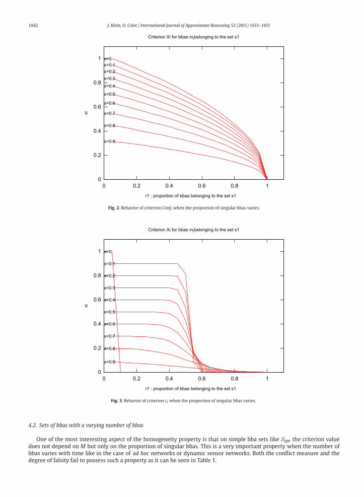
several values of x. The same curves are obtained for the set s2. Fig. 2 shows the non-linearity of criterion Confi with

respect to r1 for several values of x. The same curves are obtained for the set s2. It can be shown that Conf 2i is linear with

respect to r1. Consequently, if one chooses g (r) = √r, g (ξi) is an adapted criterion whose behavior is close to Confi.

Fig. 3 shows the non-linearity of criterion ci with respect to r1 for several values of x. The same curves are obtained for

the set s2. Regarding this experiment, criterion ci is the one whose behavior is the most difficult to predict because an

expression relating r1 to ci is hard to obtain. The value it takes appears to be rather binary depending on the fact that|s1| < |s2| or |s1| > |s2|. Note that if one chooses a sigmoid function for g (r), g (ξi) is an adapted criterion whose behavior

is likely to be close to ci. In addition, as explained in Section 3.1, the criterion ci fails when x = 0 i.e. when bbas are

categorical.

Fig. 1. Behavior of criterion ξi when the proportion of singular bbas varies.


Fig. 2. Behavior of criterion Confi when the proportion of singular bbas varies.

Fig. 3. Behavior of criterion ci when the proportion of singular bbas varies.

4.2. Sets of bbas with a varying number of bbas

One of the most interesting aspect of the homogeneity property is that on simple bba sets like Sspe the criterion value

does not depend on M but only on the proportion of singular bbas. This is a very important property when the number of

bbas varies with time like in the case of ad hoc networks or dynamic sensor networks. Both the conflict measure and the

degree of falsity fail to possess such a property as it can be seen in Table 1.


Table 1

Values of ci , Confi and ξi for several bba sets of type Sspe with a varying size M. The proportion of singular bbas is r = 0.25. All bbas are

identically committed and |Ω| = 3. – means that the criterion could not be computed because the machine precision was reached.

bba set of type Sspe with∣∣Sspe

∣∣ = Mbba type Degree of falsity ci Conflict measure Confi Criterion ξi

M=4bba mi ∈ s1, s1 =

{1× {a}m0.1

}0.79 0.89 0.48

bba mi ∈ s2, s1 ={3× {b}m0.1

}0.11 0.52 0.16

M=8bba mi ∈ s1, s1 =

{2× {a}m0.1

}0.80 0.83 0.48

bba mi ∈ s2, s1 ={6× {b}m0.1

}6.10e−3 0.48 0.16

M=16bba mi ∈ s1, s1 =

{4× {a}m0.1

}0.80 0.80 0.48

bba mi ∈ s2, s1 ={12× {b}m0.1

}1.00e−5 0.46 0.16

M=32bba mi ∈ s1, s1 =

{8× {a}m0.1

}0.80 0.79 0.48

bba mi ∈ s2, s1 ={24× {b}m0.1

}≈0 0.45 0.16

M=64bba mi ∈ s1, s1 =

{16× {a}m0.1

}– 0.78 0.48

bba mi ∈ s2, s1 ={48× {b}m0.1

}– 0.45 0.16

M=128bba mi ∈ s1, s1 =

{32× {a}m0.1

}– 0.78 0.48

bba mi ∈ s2, s1 ={96× {b}m0.1

}– 0.45 0.16

M=256bba mi ∈ s1, s1 =

{64× {a}m0.1

}– 0.78 0.48

bba mi ∈ s2, s1 ={192× {b}m0.1

}– 0.45 0.16

M=512bba mi ∈ s1, s1 =

{128× {a}m0.1

}– 0.78 0.48

bba mi ∈ s2, s1 ={384× {b}m0.1

}– 0.45 0.16

M=1024bba mi ∈ s1, s1 =

{256× {a}m0.1

}– 0.77 0.48

bba mi ∈ s2, s1 ={768× {b}m0.1

}– 0.45 0.16

Note that the dependency of Confi decreases asM increases. Again, there is a computational limit for ci whenM is large.

4.3. Sets of bbas with random masses

The two aspects highlighted in the previous subsections are only valid for a particular kind of bba sets. In broader cases,

these properties are no longer valid, however, it can be expected from criterion ξi to maintain a satisfying behavior in the

general case thanks to the homogeneity property. To compare the three criteria on a more general basis, random sets of

sbbas were generated. A randomly chosen sbba mi = Amx is obtained as follows:

• a focal set A is randomly chosen in{2Ω \Ω,∅

}(with equal probability for each subset),

• the mass assigned to this set is 1− x with x randomly chosen in [0, 1] using a uniform distribution.

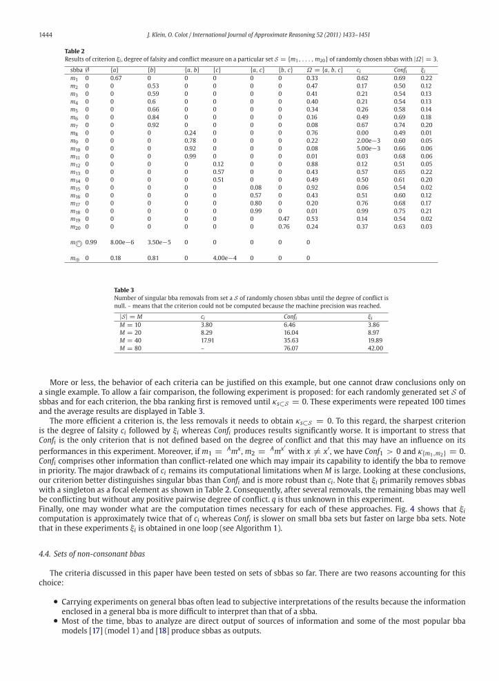
We first present aworked out example on a particular sbba set S withM = 20 in Table 2.We note that this bba set contains a

majority of bbas in favor of hypothesis b. This is pointed out by the bba combination using the conjunctive rule or Dempster’s

rule. Let us discuss the results of each criterion individually :

• the degree of falsity is the sharpest criterion. It assigns large values to bbas in direct conflict with b like m1 and m13

to m18. However a large value c7 (ranking 3) is also found for m7 = {b}m0.08 because of its strong commitment. c7exceeds c1 whereas m7 supports b.• In its raw form, Confi is the criterion with the smallest variability and appears consequently less discriminative. The

two bbas with the highest conflict measure value are m7 = {b}m0.08 and m18 = {a,c}m0.01. As m7 is in accordance

with the majority opinion, this can be seen as a dangerous behavior. Again, m7 is considered more conflicting than

m1.• Concerning criterion ξi, the smallest values are found for bbasm8 tom12,m19 andm20. These bbas have a focal element

of cardinal 2 that contains b. Like the two other criteria, m7 is assigned a rather high value but it ranks 4th and we

have ξ7 < ξ1.


Table 2

Results of criterion ξi , degree of falsity and conflict measure on a particular set S = {m1, . . . ,m20} of randomly chosen sbbas with |Ω| = 3.

sbba ∅ {a} {b} {a, b} {c} {a, c} {b, c} Ω = {a, b, c} ci Confi ξim1 0 0.67 0 0 0 0 0 0.33 0.62 0.69 0.22

m2 0 0 0.53 0 0 0 0 0.47 0.17 0.50 0.12

m3 0 0 0.59 0 0 0 0 0.41 0.21 0.54 0.13

m4 0 0 0.6 0 0 0 0 0.40 0.21 0.54 0.13

m5 0 0 0.66 0 0 0 0 0.34 0.26 0.58 0.14

m6 0 0 0.84 0 0 0 0 0.16 0.49 0.69 0.18

m7 0 0 0.92 0 0 0 0 0.08 0.67 0.74 0.20

m8 0 0 0 0.24 0 0 0 0.76 0.00 0.49 0.01

m9 0 0 0 0.78 0 0 0 0.22 2.00e−3 0.60 0.05

m10 0 0 0 0.92 0 0 0 0.08 5.00e−3 0.66 0.06

m11 0 0 0 0.99 0 0 0 0.01 0.03 0.68 0.06

m12 0 0 0 0 0.12 0 0 0.88 0.12 0.51 0.05

m13 0 0 0 0 0.57 0 0 0.43 0.57 0.65 0.22

m14 0 0 0 0 0.51 0 0 0.49 0.50 0.61 0.20

m15 0 0 0 0 0 0.08 0 0.92 0.06 0.54 0.02

m16 0 0 0 0 0 0.57 0 0.43 0.51 0.60 0.12

m17 0 0 0 0 0 0.80 0 0.20 0.76 0.68 0.17

m18 0 0 0 0 0 0.99 0 0.01 0.99 0.75 0.21

m19 0 0 0 0 0 0 0.47 0.53 0.14 0.54 0.02

m20 0 0 0 0 0 0 0.76 0.24 0.37 0.63 0.03

m ∩© 0.99 8.00e−6 3.50e−5 0 0 0 0 0

m⊕ 0 0.18 0.81 0 4.00e−4 0 0 0

Table 3

Number of singular bba removals from set a S of randomly chosen sbbas until the degree of conflict is

null. – means that the criterion could not be computed because the machine precision was reached.

|S| = M ci Confi ξiM = 10 3.80 6.46 3.86

M = 20 8.29 16.04 8.97

M = 40 17.91 35.63 19.89

M = 80 – 76.07 42.00

More or less, the behavior of each criteria can be justified on this example, but one cannot draw conclusions only on

a single example. To allow a fair comparison, the following experiment is proposed: for each randomly generated set S of

sbbas and for each criterion, the bba ranking first is removed until κs⊂S = 0. These experiments were repeated 100 times

and the average results are displayed in Table 3.

The more efficient a criterion is, the less removals it needs to obtain κs⊂S = 0. To this regard, the sharpest criterion

is the degree of falsity ci followed by ξi whereas Confi produces results significantly worse. It is important to stress that

Confi is the only criterion that is not defined based on the degree of conflict and that this may have an influence on its

performances in this experiment. Moreover, if m1 = Amx , m2 = Amx′ with x �= x′, we have Conf1 > 0 and κ{m1,m2} = 0.

Confi comprises other information than conflict-related one which may impair its capability to identify the bba to remove

in priority. The major drawback of ci remains its computational limitations when M is large. Looking at these conclusions,

our criterion better distinguishes singular bbas than Confi and is more robust than ci. Note that ξi primarily removes sbbas

with a singleton as a focal element as shown in Table 2. Consequently, after several removals, the remaining bbas may well

be conflicting but without any positive pairwise degree of conflict. q is thus unknown in this experiment.

Finally, one may wonder what are the computation times necessary for each of these approaches. Fig. 4 shows that ξicomputation is approximately twice that of ci whereas Confi is slower on small bba sets but faster on large bba sets. Note

that in these experiments ξi is obtained in one loop (see Algorithm 1).

4.4. Sets of non-consonant bbas

The criteria discussed in this paper have been tested on sets of sbbas so far. There are two reasons accounting for this

choice:

• Carrying experiments on general bbas often lead to subjective interpretations of the results because the information

enclosed in a general bba is more difficult to interpret than that of a sbba.• Most of the time, bbas to analyze are direct output of sources of information and some of the most popular bba

models [17] (model 1) and [18] produce sbbas as outputs.


Fig. 4. Computation time of criteria ci , Confi and ξi with respect to the number of bbas.

Table 4

Impact of a non-consonant bba on conflict analysis criteria.

Conflict analysis in S Conflict analysis in S ′ifmi ={a} m0.5 ifmi ={b} m0.5 ifmi ={a} m0.5 ifmi ={b} m0.5 ifmi ={a} m0.5 ∩©{b}m0.5

Raw value Percent Raw value Percent Raw value Percent Raw value Percent Raw value Percent

ξi 7.49e−3 10.00 2.50e−3 3.33 7.65e−6 1.30 2.51e−6 0.40 5.35e−4 89.00

Confi 0.28 7.30 0.16 4.20 0.28 7.90 0.16 4.40 0.25 8.00

ci 7.17e−2 12.70 1.37e−2 2.40 7.17e−2 12.80 1.37e−2 2.40 8.16e−2 14.60

Nonetheless, there exists models producing more general bbas [19,20] or [17] (model 2) and futhermore, evaluating bbas

arising from combination process may also be of great importance. It is therefore interesting to observe the behavior of

the criteria when processing general bbas and to examine if their performances may degrade. Among non-simple bbas, we

will only focus on a special kind of bbas that are non-consonant bbas. This type of bbas is the only one likely to provoke

unforeseen issues. Indeed, a non-consonant bba is such that it has two focal elements A and B with A ∩ B = ∅. In other

words, there is some conflict encoded within the bba.

To understand the impact of a non-consonant bba on the criteria, let us carry this simple experiment: let us consider a

set S of 20 sbbas. Suppose 5 of them are equal to {a}m0.5 and the 15 remaining ones are equal to {b}m0.5. We already know

how the three criteria respond to this situation. Now, let us process another bba set S′ that contains 19 bbas. 4 of them are

equal to {a}m0.5 and 14 of them are equal to {b}m0.5 and the 19th one is equal to {a}m0.5 ∩©{b}m0.5.

Formally, the two sets contain the same pieces of evidence, but these pieces are not distributed the sameway. The results

for the three criteria are presented in Table 4.

In this experiment, it can be argued that each criterion produces a satisfactory response in its way. Indeed, for both the

degree of falsity and the conflict measure, the raw values remain nearly unchanged and this can be regarded as normal

since the same pieces of evidence are considered in both cases. In addition, the non-consonant bba is given a degree of

falsity or conflict measure that is slightly higher than the singular bbas (i.e. when mi = {a}m0.5). The criterion ξi has a

dramatically different behavior in the sense that the non-consonant bba drags 89% of the estimated conflict. This is perfectly

well understood when one looks at Eq. (29). The non-consonant bba is the only one that has a positive pairwise degree

of conflict with all other bba of S ′ and its value is a lot higher. This can be also regarded as an interesting result because

non-consonant bba can be viewed as contradictory bba that deserves a to be processed in priority.

4.5. Concluding remarks on the experiments

Throughout this section, theproposed conflict analysis criterion ξi has been compared to two state-of-the-art approaches:

the degree of falsity ci and the conflict measure Confi. The experiments in Sections 4.1 and 4.2 have pointed out that ξi


offers some possibilities beyond reach of the two other criteria. These possibilities are expressed via the homogeneity

property.

In terms of performances, it cannot be concluded that one of the criteria outperforms the other ones in all situations.

Looking at the experiments in Sections 4.3, ξi should be preferred when the number of bbas is large but when it is small, ciobtains slightly better performances. Confi appears to be less efficient when one intends to get rid of the most conflicting

bbas but if another goal is sought, it may reveal itself as efficient as the two other ones. Moreover, ξi turns out to be useful

when it is intended to mine non-consonant bbas in priority as shown in Section 4.4.

The collectionof the remarks andconsiderations above justify thepractical interest of our contribution.Note that although

non-consonant bbas are studied in the experiment of Section 4.4, most of the the results presented in this study are obtained

onthespecial caseof simplesupportbbas. It is therefore important tooutline that conflict evaluationcriteriamaybeusedwith

caution on sets of more general bbas simply because defining what is conflictual in such bbas is a much more complex task.

5. Conclusion

In this article, the way bbas conflict with one another has been studied under a new perspective. Viewing the degree of

conflict as a function of discounting rates has led to newdevelopments and the introduction of a newcriterion assessing a bba

contribution to the conflict. As compared to existing approaches, this criterion appears to be more robust to parameters like

the proportion of conflicting bbas and thenumber of bbaswith a better or equivalent efficiency. In addition the interpretation

and the justification of this criterion are easily understood.

Various perspectives arise from this contribution on both theoretical and practical grounds. Concerning theoretical as-

pects, wewould like to further investigate the relationship between sub-degrees of conflict in connectionwith recent works

on the discounting operation [12]. We would like also to investigate how this criterion could be re-injected inside a combi-

nation rule, Liu et al. [21] have recently proposed an approach following this idea but using another criterion. Furthermore,

this study is mainly focussed on the analysis of simple support bbas and other developments are necessary to characterize

more accurately the conflict between more general bbas.

We also intend to demonstrate the interest of this criterion through real-world problems. Detecting conflicting bbas

allows to identify singular sources of information. These kind of sources correspond to deficient sources or to sources that

collected a piece of information that cannot be perceived by the others. Concerning outlier detection, the criterion could be

used to analyze datasets and mine data points of particular interest. Outlier detection is also essential in sensor networks.

Some sensors may indeed be faulty or used in some conditions for which they are not calibrated, thus yielding unreliable

information. Our criterion would be particularly useful in networks with a varying number of information sources.

Appendix A. Proofs of propositions

This appendix contains the proofs of the propositions presented in this article.

A.1. Proof of Proposition 1

∀S ⊂ BΩ , |S| = M, ∀�α ∈ [0, 1]M , we have

∂κS∂αi

(�α) = ∂

∂αi

( ∩©M

j=1mαj

j

)(∅) (A.1)

Following the definition of the conjunctive rule, the expression becomes

∂κS∂αi

(�α) = ∂

∂αi

∑∀j,Bj⊆Ω

∩Mj=1Bj=∅

mα1

1 (B1)× · · · × mαMM (BM) (A.2)

Using the definition of the discounting operation on bba mi, we get

∂κS∂αi

(�α) = ∂

∂αi

⎧⎪⎪⎪⎪⎨⎪⎪⎪⎪⎩

∑∀j,Bj⊆Ω

∩Mj=1Bj=∅,Bi �=Ω

mα1

1 (B1)× · · · × (1− αi)mi (Bi)× · · · × mαMM (BM)

+ ∑∀j,Bj⊆Ω

∩Mj=1Bj=∅Bi=Ω

mα1

1 (B1)× · · · × ((1− αi)mi (Ω)+ αi)× · · · × mαMM (BM)

⎫⎪⎪⎪⎪⎪⎪⎬⎪⎪⎪⎪⎪⎪⎭


These sums can be re-organized as follows:

∂κS∂αi

(�α) = ∂

∂αi

⎧⎨⎩(1− αi)

∑∀j,Bj⊆Ω,

∩Mj=1Bj=∅

mα1

1 (B1)× · · · × mi (Bi)× · · · × mαMM (BM)

+αi

∑∀j �=i,Bj⊆Ω

∩Mj=1,j �=iBj=∅

mα1

1 (B1)× · · · × mαMM (BM)

⎫⎪⎪⎪⎪⎬⎪⎪⎪⎪⎭

= ∂

∂αi

{(1− αi) κS (�α − αi�ei)+ αiκS\{mi}

(pS\{mi} (�α)

)}(A.3)

Since κS (�α − αi�ei) and κS\{mi}(pS\{mi} (�α)

)are both independent from the variable αi, using derivation rules, we obtain

∂κS∂αi

(�α) = −κS (�α − αi�ei)+ κS\{mi}(pS\{mi} (�α)

)(A.4)


Proof by recurrence on the number M of bbas:

• Lets us first examine Proposition 2 for M = 2: S = {m1,m2}. In this case, the degree of conflict writes as:

κS (α1, α2) =∑

B1,B2⊆Ω

B1∩B2=∅

mα1

1 (B1)mα2

2 (B2) (A.5)

Using the definition of the discounting operation on bba m1, we get

κS (α1, α2)=∑

B1,B2⊆Ω

B1∩B2=∅B1 �=Ω

(1− α1)m1 (B1)mα2

2 (B2)

+ ∑B1,B2⊆Ω

B1∩B2=∅B1=Ω

[(1− α1)m1 (Ω)+ α1]mα2

2 (B2)

These sums can be re-organized as follows:

κS (α1, α2)= (1− α1)∑

B1,B2⊆Ω

B1∩B2=∅

m1 (B1)mα2

2 (B2)

+α1

∑B2⊆Ω

Ω∩B2=∅

mα2

2 (B2)

The second sum reduces to a single term as the only subset B2 of Ω such that B2 ∩Ω = ∅ is B2 = ∅:κS (α1, α2) = (1− α1)

∑B1,B2⊆Ω

B1∩B2=∅

m1 (B1)mα2

2 (B2)+ α1mα2

2 (∅)

= (1− α1)∑

B1,B2⊆Ω

B1∩B2=∅

m1 (B1)mα2

2 (B2)+ α1 (1− α2)m2 (∅)

For the remaining sum, one can apply the same process as above on bba m2, and we thus have:

κS (α1, α2) = (1− α1)

⎡⎢⎢⎣(1− α2)

∑B1,B2⊆Ω

B1∩B2=∅

m1 (B1)m2 (B2)+ α2m2 (∅)⎤⎥⎥⎦+ α1 (1− α2)m2 (∅)


By definition of function κs, this expression writes as:

κS (α1, α2) = (1− α1) (1− α2) κS + (1− α1) α2κ{m1} + α1 (1− α2) κ{m2}Finally, following the definition of function fs, we get

κS (α1, α2) = fS (α1) fS (α2) κS + f{m1} (α1) f{m1} (α2) κ{m1} + f{m2} (α1) f{m2} (α2) κ{m2}The proposition is thus verified for M = 2.

• Let us now investigate Proposition 2 at rankM + 1 supposing that the it is verified at rankM (i.e. for any set s of bbas in

S = {m1, . . . ,mM+1} such that |s| = M). We have

κS (�α) =( ∩©M+1

j=1 mαj

j

)(∅) (A.6)

= ∑∀j,Bj⊆Ω

∩M+1j=1 Bj=∅

mα1

1 (B1)× · · · × mαM+1M+1 (BM+1)

with �α = (α1, . . . , αM+1). Using the same idea as in the case of M = 2, the expression can be expanded using the

definition of the discounting operation on bba mM+1 :

κS (�α)= ∑∀j,Bj⊆Ω

∩M+1j=1 Bj=∅BM+1 �=Ω

mα1

1 (B1)× · · · × (1− αM+1)mM+1 (BM+1)

+ ∑∀j,Bj⊆Ω

∩M+1j=1 Bj=∅BM+1=Ω

mα1

1 (B1)× · · · × [(1− αM+1)mM+1 (Ω)+ αM+1]

= (1− αM+1)∑∀j,Bj⊆Ω

∩M+1j=1 Bj=∅

mα1

1 (B1)× · · · × mM+1 (BM+1)

+αM+1∑∀j,Bj⊆Ω

∩Mj=1Bj=∅

mα1

1 (B1)× · · · × mαMM (BM)

= (1− αM+1) κS (α1, . . . , αM, 0)+ αM+1κS\{mM+1} (α1, . . . , αM) (A.7)

In the expression above, the problem comes from the term κS (α1, . . . , αM, 0) which remains a function of the M + 1

variables. However, the same expansion can be applied to this term using the discounting operation definition for bba

mM and because the result obtained by Eq. (A.7) is true ∀�α ∈ [0, 1]M+1. We can thus write

κS (α1, . . . , αM, 0)= (1− αM) κS (α1, . . . , αM−1, 0, 0) (A.8)

+αMκS\{mM} (α1, . . . , αM−1, 0) (A.9)

Onemaynote that the term κS\{mM} (α1, . . . , αM−1, 0) is a function of the followingM variables: {α1, . . . , αM−1, αM+1}(the value of αM+1 being 0 in this case).

Now expression (A.9) can be inserted within expression (A.7) and we have

κS (�α)= (1− αM+1) (1− αM) κS (α1, . . . , αM−1, 0, 0)+ (1− αM+1) αMκS\{mM} (α1, . . . , αM−1, 0)+αM+1κS\{mM+1} (α1, . . . , αM) (A.10)

The principle used to obtain expression (A.10) can be iterated M times so as to obtain:

κS (�α) =M+1∏i=1

(1− αi) κS(�0)

+α1

M+1∏i=2

(1− αi) κS\{m1} (0, . . . , 0)+ · · ·


+αj

M+1∏i=j

(1− αi) κS\{mj}(α1, . . . , αj−1, 0, . . . , 0

)+ · · ·+αM+1κS\{mM+1} (α1, . . . , αM) (A.11)

which can be written in a more condensed form as

κS (�α) =M+1∏i=1

(1− αi) κS(�0)

+M+1∑j=1

αj

M+1∏i=j

(1− αi) κS\{mj}(α1, . . . , αj−1, 0, . . . , 0

)(A.12)

Now we can use the hypothesis of recurrence at rank M for all the terms of the type κS\{mj}(α1, . . . , αj−1, 0, . . . , 0

).

Indeed, we have

κS\{mj}(α1, . . . , αj−1, 0, . . . , 0

) = ∑s⊆S\{mj},s �=∅

κs

j−1∏i=1

fs (αi)M+1∏i=j+1

fs (0) (A.13)

Considering that fs (0) =⎧⎨⎩ 0 if i /∈ s

1 if i ∈ s, all sets s that do not include

{mj+1, . . . ,mM+1

}can be discarded. We thus have

κS\{mj}(α1, . . . , αj−1, 0, . . . , 0

) = ∑s⊆{m1,...,mj−1},s �=∅

κs∪{mj+1,...,mM+1}j−1∏i=1

fs∪{mj+1,...,mM+1} (αi) (A.14)

Expression (A.14) can be inserted in Eq. (A.12):

κS (�α)=M+1∏i=1

(1− αi) κS(�0)

+M+1∑j=1

αj

M+1∏i=j

(1− αi)∑

s⊆{m1,...,mj−1},s �=∅κs∪{mj+1,...,mM+1}

j−1∏i=1

fs∪{mj+1,...,mM+1} (αi)

By definition of function fs, fs∪{mj+1,...,mM+1}(αj

) = αj because mj /∈ s ∪ {mj+1, . . . ,mM+1}. Similarly, ∀i > j

fs∪{mj+1,...,mM+1} (αi) = 1 − αi, because i ∈ s ∪ {mj+1, . . . ,mM+1}and ∀i fS (αi) = 1 − αi because mi ∈ S . Con-

sequently, we obtain

κS (�α)= κSM+1∏i=1

fS (αi)

+M+1∑j=1

∑s⊆{m1,...,mj−1},s �=∅

κs∪{mj+1,...,mM+1}M+1∏i=1

fs∪{mj+1,...,mM+1} (αi)

Let us now investigate the sets indexed as s ∪ {mj+1, . . . ,mM+1}in the double-sum in the expression above so as to

determine if they can be re-organized. Let A be the set of all subsets of S except S itself:

A = {s � S} . (A.15)

Let B the set that contains all sets of type s ∪ {mj+1, . . . ,mM+1}indexed in the double-sum:

B = ∪M+1j=1{s ∪ {mj+1, . . . ,mM+1

}with s ⊆ {m1, . . . ,mj−1

}}. (A.16)

Now let us compare A with B:

– A is the set of all subsets of S except S itself. B is composed of such subsets, therefore, clearly we have B ⊆ A.

– Looking at the double sum for j = M + 1, we note that, we have AM+1 = {s ⊆ {m1, . . . ,mM}} ⊆ B. This result

is independent from the order with which the bbas are processed, so if one switches bba mM+1 with bba mi using

a permutation, the double sum remains identical and we have Ai ⊆ B. Consequently, ∀i, Ai ⊆ B, which implies

∪M+1i=1 Ai ⊆ B which by definition of A is equivalent to A ⊆ B.

– Finally, since B ⊆ A and A ⊆ B, we conclude A = B.


We thus obtain

κS (�α)= κSM+1∏i=1

fS (αi)

+ ∑s�S,s �=∅

κs

M+1∏i=1

fs (αi)

= ∑s⊆S,s �=∅

κs

M+1∏i=1

fs (αi) (A.17)

The hypothesis is thus verified at rank M + 1 which concludes the proof of Proposition 2.


Proof by recurrence on the number n of discounting operations with rates 12�u:

• Lets us first examine Proposition 4 for n = 1: we have

γM1 (x)= (2− 1)M−x

2M(A.18)

= 1

2M

This case reduces to Corollary 1, it is thus verified.• Let us now investigate Proposition 4 at rank n+ 1 supposing that the it is verified at rank n. The result at rank 1 can

be used on κS([

1−(12

)n+1] �u) to obtain

κS

([1−

(1

2

)n+1]�u)= ∑

s⊆S,s �=∅γM1 (|s|) κs

([1−

(1

2

)n]�u)

Using the hypothesis at rank n, we can write

κS

([1−

(1

2

)n+1]�u)= ∑

s⊆S,s �=∅γM1 (|s|) ∑

s′⊆s,s′ �=∅γMn

(∣∣∣s′∣∣∣) κs′ (A.19)

The expression above is a weighed sum of sub-degrees of conflict, it can thus be re-written as∑

s⊆S γMn+1 (|s|) κs

where γMn+1 (|s|) are weights to determine. The values of weights can be found by analyzing expression A.19. Let us

separate this analysis for different values of∣∣s′∣∣ and count how many times each term κs′ occurs:

– when∣∣s′∣∣ = M, there is only one possible choice: s′ = s = S . We conclude

γMn+1 (M)= γM

1 (M) γMn (M)

= 1

2M× 1

2nM

= 1

2(n+1)M . (A.20)

– when∣∣s′∣∣ = M − 1, there are two possible choice for s. The term κs′ is found behind the coefficient:

* γM1 (M) γM

n (M − 1) one time (case s = S),* γM

1 (M − 1) γM−1n (M − 1) one time (case s = s′).

We conclude

γMn+1 (M − 1)= γM

1 (M) γMn (M − 1)+ γM

1 (M − 1) γM−1n (M − 1)

= 1

2M× 2n − 1

2nM+ 1

2M× 1

2n(M−1)

= 2n+1 − 1

2(n+1)M . (A.21)


– when∣∣s′∣∣ = M − i with 0 < i < M − 1 (general case), the term κs′ is found C

ji times behind the coefficient

γM1 (M − j) γ

M−jn (M − i) with j such that |s| = M − j and C

ji the binomial coefficient (number of choices if j

items among i). This statement is true for j varying from 0 to i. We can thus write

γMn+1 (M − i) =

i∑j=0

Cjiγ

M1 (M − j) γM−j

n (M − i)

=i∑

j=0Cji

1

2M

(2n − 1)M−j−(M−i)

2n(M−j)

= 1

2M(n+1)i∑

j=0Cji

(2n − 1

)i−j (2n)j

= 1

2M(n+1)(2n − 1+ 2n

)i

=(2n+1 − 1

)i2M(n+1) (A.22)

The result above is equivalent to γMn+1 (|s|) = (2n+1−1)M−|s|

2M(n+1) . Consequently, the hypothesis is verified at rank

n+ 1, which concludes the proof of Proposition 4.

Appendix B. Example of a bba set with a positive global degree of conflict but without any positive pairwise degree of

conflict

Let Ω = {a, b, c} be a frame of discernment. Suppose one has obtained the following bba set: S = {m1,m2,m3}with:

• m1 = {a,b}mx ,• m2 = {a,c}mx ,• m3 = {b,c}mx ,• x ∈]0, 1].

We have κS > 0 but κ{m1,m2} = κ{m1,m3} = κ{m2,m3} = 0.

References

[1] A. Dempster, Upper and lower probabilities induced by a multiple valued mapping, Annals of Mathematical Statistics 38 (1967) 325–339.

[2] G. Shafer, A Mathematical Theory of Evidence, Princeton University press, Princeton (NJ), USA, 1976.[3] P. Smets, Analyzing the combination of conflicting belief functions, Information Fusion 8 (2007) 387–412.

[4] V.J. Hodge, J. Austin, A survey of outlier detection methodologies, Artificial Intelligence Review 22 (2004) 85–126.[5] A. Martin, A.-L. Jouselme, C. Osswald, Conflict measure for the discounting operation on belief functions, in: Proceedings of the Eleventh International

Conference on Information Fusion, 2008, pp. 1–8.[6] J. Schubert, Specifying nonspecific evidence, International Journal of Intelligent Systems 11 (1996) 525–563.

[7] J. Schubert, Conflictmanagement in Dempster–Shafer theory using the degree of falsity, International Journal of Approximate Reasoning 52 (2010) 449–460.

[8] J. Klein, C. Lecomte, P. Miché, Hierarchical and conditional combination of belief functions induced by visual tracking, International Journal of ApproximateReasoning 51 (2009) 410–428.

[9] K. Sentz, S. Ferson, Combination of evidence in Dempster–Shafer theory, Tech. Rep. SAND2002-0835, Sandia National Laboratories, 2002.[10] D. Mercier, B. Quost, T. Denoeux, Refined modeling of sensor reliability in the belief function framework using contextual discounting, Information Fusion

9 (2008) 246–258.[11] A. Kallel, S.L. Hégarat-Mascle, Combination of partially non-distinct beliefs: the cautious-adaptative rule, International Journal of Approximate Reasoning

50 (2009) 1000–1021.[12] D. Mercier, E. Lefevre, F. Delmotte, Belief functions contextual discounting and canonical decompositions, International Journal of Approximate Reasoning,

(2011), in press, doi:10.1016/j.ijar.2011.06.005.

[13] P. Zhang, I. Gardin, P. Vannoorenberghe, Information fusion using evidence theory for segmentation of medical images, in: International Colloquium onInformation Fusion, Xi’an, PR China, 2007, pp. 265–272.

[14] W. Li, A. Joshi, Outlier detection in ad hoc networks usingDempster–Shafer theory, in: Tenth International Conference onMobile DataManagement: Systems,Services and Middleware, Los Alamitos (CA), USA, 2009, pp. 112–121.

[15] S. Panigrahi, A. Kundu, S. Sural, A.Majumdar, Credit card frauddetection: a fusion approachusingDempster–Shafer theory andBayesian learning, InformationFusion 10 (2009) 354–363.

[16] A.-L. Jousselme, D. Grenier, E. Bossé, A new distance between two bodies of evidence, Information Fusion 2 (2001) 91–101.

[17] A. Appriou, Probabilités et incertitude en fusion de données multi-senseurs, Revue scientifique de la defense 11 (1991) 27–40.[18] T. Denoeux, A k-nearest neighbour classification rule based on Dempster–Shafer theory, IEEE Transactions on Systems Man and Cybernetics 25 (5) (1995)

804–813.[19] G. Shafer, R. Logan, Implementing Dempster’s rule for hierarchical evidence, Artificial Intelligence 33 (1987) 271–298.

[20] L. Xu, A. Krzyzak, C.Y. Suen,Methods of combiningmultiple classifiers and their applications to handwriting recognition, IEEE Transactions on Systems,Man,and Cybernetics 22 (1992) 418–435.

[21] Z.-G. Liu, Q. Pan, Y.-M. Cheng, J. Dezert, Sequential adaptive combination of unreliable sources of evidence, in: Proceedings of the Workshop on the Theory

of Belief Functions, Brest, France, 2010, pp. 1–6 (paper 89).

doi:10.1016/j.ijar.2011.06.005

Singular sources mining using evidential conflict analysis

Documents

Transcript of Singular sources mining using evidential conflict analysis