Single Variable Minimization - Stanford...

AA222: MDO 37 Sunday 1st April, 2012 at 19:48

Chapter 2

Single Variable Minimization

2.1 Motivation

Most practical optimization problems involve many variables, so the study of single variable mini-mization may seem academic. However, the optimization of multivariable functions can be brokeninto two parts: 1) finding a suitable search direction and 2) minimizing along that direction. Thesecond part of this strategy, the line search, is our motivation for studying single variable mini-mization.

Consider a scalar function f : R → R that depends on a single independent variable, x ∈ R.Suppose we want to find the value of x where f(x) is a minimum value. Furthermore, we want todo this with

• low computational cost (few iterations and low cost per iteration),

• low memory requirements, and

• low failure rate.

Often the computational effort is dominated by the computation of f and its derivatives so someof the requirements can be translated into: evaluate f(x) and df/dx as few times as possible.

2.2 Optimality Conditions

We can classify a minimum as a:

1. Strong local minimum

2. Weak local minimum

3. Global minimum

As we will see, Taylor’s theorem is useful for identifying local minima. Taylor’s theorem statesthat if f(x) is n times differentiable, then there exists θ ∈ (0, 1) such that

f(x+ h) = f(x) + hf ′(x) +1

2h2f ′′(x) + · · ·+ 1

(n− 1)!hn−1fn−1(x) +

1

n!hnfn(x+ θh)︸︷︷︸O(hn)

(2.1)


Now we assume that f is twice-continuously differentiable and that a minimum of f exists atx∗. Then, using n = 2 and x = x∗ in Taylor’s theorem we obtain,

f(x∗ + ε) = f(x∗) + εf ′(x∗) +1

2ε2f ′′(x∗ + θε) (2.2)

For x∗ to be a local minimizer, we require that f(x∗+ε) ≥ f(x∗) for a range −δ ≤ ε ≤ δ, whereδ is a positive number. Given this definition, and the Taylor series expansion (2.2), for f(x∗) to bea local minimum, we require

εf ′(x∗) +1

2ε2.f ′′(x∗ + θε) ≥ 0 (2.3)

For any finite values of f ′(x∗) and f ′′(x∗), we can always chose a ε small enough such that εf ′(x∗)�12ε

2f ′′(x∗). Therefore, we must consider the first derivative term to establish under which conditionswe can satisfy the inequality (2.3).

For εf ′(x∗) to be non-negative, then f ′(x∗) = 0, because the sign of ε is arbitrary. This is thefirst-order optimality condition. A point that satisfies the first-order optimality condition is calleda stationary point.

Because the first derivative term is zero, we have to consider the second derivative term. Thisterm must be non-negative for a local minimum at x∗. Since ε2 is always positive, then we requirethat f ′′(x∗) ≥ 0. This is the second-order optimality condition. Terms higher than second ordercan always be made smaller than the second-order term by choosing a small enough ε.

Thus the necessary conditions for a local minimum are:

f ′(x∗) = 0; f ′′(x∗) ≥ 0 (2.4)

If f(x∗ + ε) > f(x∗), and the “greater or equal than” in the required inequality (2.3) canbe shown to be greater than zero (as opposed to greater or equal), then we have a strong localminimum. Thus, sufficient conditions for a strong local minimum are:

f ′(x∗) = 0; f ′′(x∗) > 0 (2.5)

The optimality conditions can be used to:

1. Verify that a point is a minimum (sufficient conditions).

2. Realize that a point is not a minimum (necessary conditions).

3. Define equations that can be solved to find a minimum

Gradient-based minimization methods find a local minima by finding points that satisfy theoptimality conditions.

2.3 Numerical Precision

Solving the first-order optimality conditions, that is, finding x∗ such that f ′(x∗) = 0, is equivalentto finding the roots of the first derivative of the function to be minimized. Therefore, root findingmethods can be used to find stationary points and are useful in function minimization.

Using machine precision, it is not possible find the exact zero, so we will be satisfied with findingan x∗ that belongs to an interval [a, b] such that the function g satisfies

g(a)g(b) < 0 and |a− b| < δ (2.6)

where δ is a “small” tolerance. This tolerance might be dictated by the machine representation(using double precision this is usually 1×10−16), the precision of the function evaluation, or a limiton the number of iterations we want to perform with the root finding algorithm.


2.4 Convergence Rate

Optimization algorithms compute a sequence of approximate solutions that we hope converges tothe solution. Two questions are important when considering an algorithm:

• Does it converge?

• How fast does it converge?

Suppose you we have a sequence of points xk (k = 1, 2, . . .) converging to a solution x∗. For aconvergent sequence, we have

limk→∞

xk − x∗ = 0 (2.7)

The rate of convergence is a measure of how fast an iterative method converges to the numericalsolution. An iterative method is said to converge with order r when r is the largest positive numbersuch that

0 ≤ limk→∞

‖xk+1 − x∗‖‖xk − x∗‖r

<∞. (2.8)

For a sequence with convergence rate r, asymptotic error constant, γ is the limit above, i.e.

γ = limk→∞

‖xk+1 − x∗‖‖xk − x∗‖r

. (2.9)

To understand this better, lets assume that we have ideal convergence behavior so that condi-tion (2.9) is true for every iteration k+ 1 and we do not have to take the limit. Then we can write

‖xk+1 − x∗‖ = γ‖xk − x∗‖r for all k. (2.10)

The larger r is, the faster the convergence. When r = 1 we have linear convergence, and ‖xk+1 −x∗‖ = γ‖xk − x∗‖. If 0 < γ < 1, then the norm of the error decreases by a constant factor forevery iteration. If γ > 1, the sequence diverges. When we have linear convergence, the number ofiterations for a given level of convergence varies widely depending on the value of the asymptoticerror constant.

If γ = 0 when r = 1, we have a special case: superlinear convergence. If r = 1 and γ = 1, wehave sublinear convergence.

When r = 2, we have quadratic convergence. This is highly desirable, since the convergenceis rapid and independent of the asymptotic error constant. For example, if γ = 1 and the initialerror is ‖x0−x∗‖ = 10−1, then the sequence of errors will be 10−1, 10−2, 10−4, 10−8, 10−16, i.e., thenumber of correct digits doubles for every iteration, and you can achieve double precision in fouriterations!

For n dimensions, x is a vector with n components and we have to rethink the definition of theerror. We could use, for example, ||xk − x∗||. However, this depends on the scaling of x, so weshould normalize with respect to the norm of the current vector, i.e.

||xk − x∗||||xk||

. (2.11)

One potential problem with this definition is that xk might be zero. To fix this, we write,

||xk − x∗||1 + ||xk||

. (2.12)


Another potential problem arises from situations where the gradients are large, i.e., even if we havea small ||xk − x∗||, |f(xk)− f(x∗)| is large. Thus, we should use a combined quantity, such as,

||xk − x∗||1 + ||xk||

+|f(xk)− f(x∗)|

1 + |f(xk)|(2.13)

Final issue is that when we perform numerical optimization, x∗ is usually not known! However,you can monitor the progress of your algorithm using the difference between successive steps,

||xk+1 − xk||1 + ||xk||

+|f(xk+1)− f(xk)|

1 + |f(xk)|. (2.14)

Sometimes, you might just use the second fraction in the above term, or the norm of the gradient.You should plot these quantities in a log-axis versus k.

2.5 Method of Bisection

Bisection is a bracketing method. This class of methods generate a set of nested intervals and requirean initial interval where we know there is a solution.

In this method for finding the zero of a function f , we first establish a bracket [x1, x2] for whichthe function values f1 = f(x1) and f2 = f(x2) have opposite sign. The function is then evaluatedat the midpoint, x = 1

2(x1 + x2). If f(x) and f1 have opposite signs, then x and f become x2 andf2 respectively. On the other hand, if f(x) and f1 have the same sign, then x and f become x1

and f1. This process is then repeated until the desired accuracy is obtained.For an initial interval [x1, x2], bisection yields the following interval at iteration k,

δk =x1 − x2

2k(2.15)

Thus to achieve a specified tolerance δ, we need log2(x1 − x2)/δ evaluations.Bisection yields the smallest interval of uncertainty for a specified number of function evalua-

tions, which is the best you can do for a first order root finding method. From the definition ofrate of convergence, for r = 1,

limk→∞

=δk+1

δk=

1

2(2.16)

Thus this method converges linearly with asymptotic error constant γ = 1/2.To find the minimum of a function using bisection, we would evaluate the derivative of f at

each iteration, instead of the value.

2.6 Newton’s Method for Root Finding

Newton’s method for finding a zero can be derived from the Taylor’s series expansion about thecurrent iteration xk,

f(xk+1) = f(xk) + (xk+1 − xk)f ′(xk) +O((xk+1 − xk)2) (2.17)

Ignoring the terms higher than order two and assuming the function next iteration to be the root(i.e., f(xk+1) = 0), we obtain,

xk+1 = xk −f(xk)

f ′(xk). (2.18)


9.4 Newton-Raphson Method Using Derivative 357

Sample page from

NUMERICAL RECIPES IN FO

RTRAN 77: THE ART OF SCIENTIFIC CO

MPUTING

(ISBN 0-521-43064-X)Copyright (C) 1986-1992 by Cam

bridge University Press.Programs Copyright (C) 1986-1992 by Num

erical Recipes Software. Perm

ission is granted for internet users to make one paper copy for their own personal use. Further reproduction, or any copying of m

achine-readable files (including this one) to any servercom

puter, is strictly prohibited. To order Numerical Recipes books

or CDROM

s, visit websitehttp://www.nr.com

or call 1-800-872-7423 (North America only),or send em

ail to directcustserv@cam

bridge.org (outside North America).

1

2

3x

f (x)

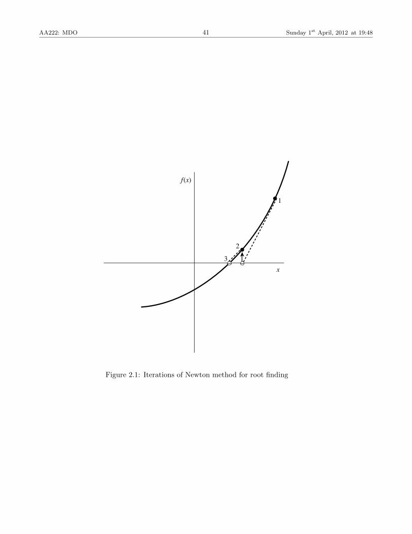
Figure 9.4.1. Newton’s method extrapolates the local derivative to find the next estimate of the root. Inthis example it works well and converges quadratically.

f (x)

x

1

23

Figure 9.4.2. Unfortunate case where Newton’s method encounters a local extremum and shoots off toouter space. Here bracketing bounds, as in rtsafe, would save the day.

Figure 2.1: Iterations of Newton method for root finding


9.4 Newton-Raphson Method Using Derivative 357

Sample page from



MPUTING







or CDROM





1

2

3x

f (x)

Figure 9.4.1. Newton’s method extrapolates the local derivative to find the next estimate of the root. Inthis example it works well and converges quadratically.

f (x)

x

1

23

Figure 9.4.2. Unfortunate case where Newton’s method encounters a local extremum and shoots off toouter space. Here bracketing bounds, as in rtsafe, would save the day.

358 Chapter 9. Root Finding and Nonlinear Sets of Equations

Sample page from



MPUTING







or CDROM





x

f (x)

2

1

Figure 9.4.3. Unfortunate case where Newton’s method enters a nonconvergent cycle. This behavioris often encountered when the function f is obtained, in whole or in part, by table interpolation. Witha better initial guess, the method would have succeeded.

This is not, however, a recommended procedure for the following reasons: (i) Youare doing two function evaluations per step, so at best the superlinear order ofconvergence will be only

√2. (ii) If you take dx too small you will be wiped out

by roundoff, while if you take it too large your order of convergence will be onlylinear, no better than using the initial evaluation f ′(x0) for all subsequent steps.Therefore, Newton-Raphsonwith numerical derivatives is (in one dimension) alwaysdominated by the secant method of §9.2. (In multidimensions, where there is apaucity of available methods, Newton-Raphson with numerical derivatives must betaken more seriously. See §§9.6–9.7.)

The following subroutine calls a user supplied subroutine funcd(x,fn,df)which returns the function value as fn and the derivative as df. We have includedinput bounds on the root simply to be consistent with previous root-finding routines:Newton does not adjust bounds, and works only on local information at the pointx. The bounds are used only to pick the midpoint as the first guess, and to rejectthe solution if it wanders outside of the bounds.

FUNCTION rtnewt(funcd,x1,x2,xacc)INTEGER JMAXREAL rtnewt,x1,x2,xaccEXTERNAL funcdPARAMETER (JMAX=20) Set to maximum number of iterations.

Using the Newton-Raphson method, find the root of a function known to lie in the interval[x1, x2]. The root rtnewt will be refined until its accuracy is known within ±xacc. funcdis a user-supplied subroutine that returns both the function value and the first derivativeof the function at the point x.

INTEGER jREAL df,dx,f

Figure 2.2: Cases where the Newton method fails

This iterative procedure converges quadratically, so

limk→∞

|xk+1 − x∗||xk − x∗|2

= const. (2.19)

While having quadratic converge is a desirable property, Newton’s method is not guaranteedto converge, and only works under certain conditions. Two examples where this method fails areshown in Figure 2.2.

To minimize a function using Newton’s method, we simply substitute the function for its firstderivative and the first derivative by the second derivative,

xk+1 = xk −f ′(xk)

f ′′(xk). (2.20)

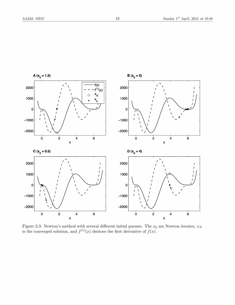
Example 2.1. Function Minimization Using Newton’s MethodConsider the following single-variable optimization problem

minimize f(x) = (x− 3)x3(x− 6)4

w.r.t. x

Solve this using Newton’s method. The results are shown in Figure ??

2.7 Secant Method

Newton’s method requires the first derivative for each iteration (and the second derivative whenapplied to minimization). In some practical applications, it might not be possible to obtain thisderivative analytically or it might just be troublesome.

If we use a forward-difference approximation for f ′(xk) in Newton’s method we obtain

xk+1 = xk − f(xk)

(xk − xk−1

f(xk)− f(xk−1)

). (2.21)


Figure 2.3: Newton’s method with several different initial guesses. The xk are Newton iterates, xNis the converged solution, and f (1)(x) dentoes the first derivative of f(x).


which is the secant method (also known as “the poor-man’s Newton method”).Under favorable conditions, this method has superlinear convergence (1 < r < 2), with r ≈

1.6180.

2.8 Golden Section Search

The golden section method is a function minimization method, as opposed to a root finding algo-rithm. It is analogous to the bisection algorithm in that it starts with an interval that is assumedto contain the minimum and then reduces that interval.

Say we start the search with an uncertainty interval [0, 1]. We need two evaluations within theinterval to reduce the size of the interval. We do not want to bias towards one side, so choose thepoints symmetrically, say 1− τ and τ , where 0 < τ < 1.

If we evaluate two points such that the two intervals that can be chosen are the same size andone of the points is reused, we have a more efficient method. This is to say that

τ

1=

1− ττ⇒ τ2 + τ − 1 = 0 (2.22)

The positive solution of this equation is the golden ratio,

τ =

√5− 1

2= 0.618033988749895 . . . (2.23)

So we evaluate the function at 1 − τ and τ , and then the two possible intervals are [0, τ ] and[1− τ, 1], which have the same size. If, say [0, τ ] is selected, then the next two interior points wouldbe τ(1− τ) and ττ . But τ2 = 1− τ from the definition (2.22), and we already have this point!

The Golden section exhibits linear convergence.

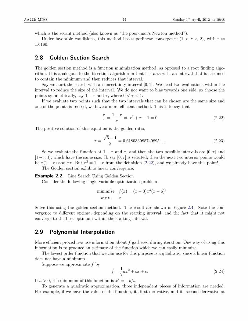
Example 2.2. Line Search Using Golden SectionConsider the following single-variable optimization problem

minimize f(x) = (x− 3)x3(x− 6)4

w.r.t. x

Solve this using the golden section method. The result are shown in Figure 2.4. Note the con-vergence to different optima, depending on the starting interval, and the fact that it might notconverge to the best optimum within the starting interval.

2.9 Polynomial Interpolation

More efficient procedures use information about f gathered during iteration. One way of using thisinformation is to produce an estimate of the function which we can easily minimize.

The lowest order function that we can use for this purpose is a quadratic, since a linear functiondoes not have a minimum.

Suppose we approximate f by

f̃ =1

2ax2 + bx+ c. (2.24)

If a > 0, the minimum of this function is x∗ = −b/a.To generate a quadratic approximation, three independent pieces of information are needed.

For example, if we have the value of the function, its first derivative, and its second derivative at


Figure 2.4: The golden section method with initial intervals [0, 3], [4, 7], and [1, 7]. The horizontallines represent the sequences of the intervals of uncertainty.

point xk, we can write a quadratic approximation of the function value at x as the first three termsof a Taylor series

f̃(x) = f(xk) + f ′(xk)(x− xk) +1

2f ′′(xk)(x− xk)2 (2.25)

If f ′′(xk) is not zero, and setting x = xk+1 this yields

xk+1 = xk −f ′(xk)

f ′′(xk). (2.26)

This is Newton’s method used to find a zero of the first derivative.

2.10 Line Search Techniques

Line search methods are related to single-variable optimization methods, as they address the prob-lem of minimizing a multivariable function along a line, which is a subproblem in many gradient-based optimization method.

After a gradient-based optimizer has computed a search direction pk, it must decide how far tomove along that direction. The step can be written as

xk+1 = xk + αkpk (2.27)

where the positive scalar αk is the step length.Most algorithms require that pk be a descent direction, i.e., that pTk gk < 0, since this guarantees

that f can be reduced by stepping some distance along this direction. The question then becomes,how far in that direction we should move.

We want to compute a step length αk that yields a substantial reduction in f , but we do notwant to spend too much computational effort in making the choice. Ideally, we would find the


Algorithm 1 Backtracking line search algorithm

Input: α > 0 and 0 < ρ < 1Output: αk

1: repeat2: α← ρα3: until f(xk + αpk) ≤ f(xk) + µ1αg

Tk pk

4: αk ← α

global minimum of f(xk + αkpk) with respect to αk but in general, it is to expensive to computethis value. Even to find a local minimizer usually requires too many evaluations of the objectivefunction f and possibly its gradient g. More practical methods perform an inexact line search thatachieves adequate reductions of f at reasonable cost.

2.10.1 Wolfe Conditions

A typical line search involves trying a sequence of step lengths, accepting the first that satisfiescertain conditions.

A common condition requires that αk should yield a sufficient decrease of f , as given by theinequality

f(xk + αpk) ≤ f(xk) + µ1αgTk pk (2.28)

for a constant 0 ≤ µ1 ≤ 1. In practice, this constant is small, say µ1 = 10−4.

Any sufficiently small step can satisfy the sufficient decrease condition, so in order to preventsteps that are too small we need a second requirement called the curvature condition, which canbe stated as

g(xk + αpk)T pk ≥ µ2g

Tk pk (2.29)

where µ1 ≤ µ2 ≤ 1, and g(xk + αpk)T pk is the derivative of f(xk + αpk) with respect to αk. This

condition requires that the slope of the univariate function at the new point be greater. Since westart with a negative slope, the gradient at the new point must be either less negative or positive.Typical values of µ2 are 0.9 when using a Newton type method and 0.1 when a conjugate gradientmethods is used.

The sufficient decrease and curvature conditions are known collectively as the Wolfe conditions.

We can also modify the curvature condition to force αk to lie in a broad neighborhood of a localminimizer or stationary point and obtain the strong Wolfe conditions

f(xk + αpk) ≤ f(xk) + µ1αgTk pk. (2.30)∣∣g(xk + αpk)

T pk∣∣ ≤ µ2

∣∣gTk pk∣∣ , (2.31)

where 0 < µ1 < µ2 < 1. The only difference when comparing with the Wolfe conditions is that wedo not allow points where the derivative has a positive value that is too large and therefore excludepoints that are far from the stationary points.

2.10.2 Sufficient Decrease and Backtracking

One of the simplest line search algorithms is the backtracking line search, listed in Algorithm 1.This algorithm in guessing a maximum step, then successively decreasing that step until the newpoint satisfies the sufficient decrease condition.


Figure 2.5: Acceptable steps for the Wolfe conditions

2.10.3 Line Search Algorithm Satisfying the Strong Wolfe Conditions

To simplify the notation, we define the univariate function

φ(α) = f(xk + αpk) (2.32)

Then at the starting point of the line search, φ(0) = f(xk). The slope of the univariate function,is the projection of the n-dimensional gradient onto the search direction pk, i.e.,

φ(α)′ = gTk pk (2.33)

This procedure has two stages:

1. Begins with trial α1, and keeps increasing it until it finds either an acceptable step length oran interval that brackets the desired step lengths.

2. In the latter case, a second stage (the zoom algorithm below) is performed that decreases thesize of the interval until an acceptable step length is found.

The first stage of this line search is detailed in Algorithm 2.

The algorithm for the second stage, the zoom(αlow, αhigh) function is given in Algorithm 3. Tofind the trial point, we can use cubic or quadratic interpolation to find an estimate of the minimumwithin the interval. This results in much better convergence that if we use the golden search, forexample.

Note that sequence {αi} is monotonically increasing, but that the order of the argumentssupplied to zoom may vary. The order of inputs for the call is zoom(αlow, αhigh), where:


2. Evaluate function value at point

1. Choose initial point

3. Does point satisfy sufficient decrease?

5. Does point satisfy the curvature condition?

4. Evaluate function derivative at point

End line search

Point is good enough

YES

3. Bracket interval between previous point and current

point

Call "zoom" function to find good point in interval

NO

YES

NO 6. Is derivative positive?

6. Bracket interval between current

point and previous point

YES

NO7. Choose new point beyond current one

"zoom" function

Figure 2.6: Line search algorithm satisfying the strong Wolfe conditions


1. Interpolate between the low value point and high value point to find a trial point in

the interval

2. Evaluate function value at trial point

3. Does trial point satisfy sufficient decrease and is less or equal than low

pointNO 3. Set point to be new high

value point

YES

4.1 Evaluate function derivative at point

4.2 Does point satisfy the curvature condition?

Point is good enough

Exit zoom (end line search)

YES

4.3 Does derivative sign at point agree with interval trend?NO 4.3 Replace high point with low

pointYES

NO

4.4 Replace low point with trial point

Figure 2.7: “Zoom” function in the line search algorithm satisfying the strong Wolfe conditions


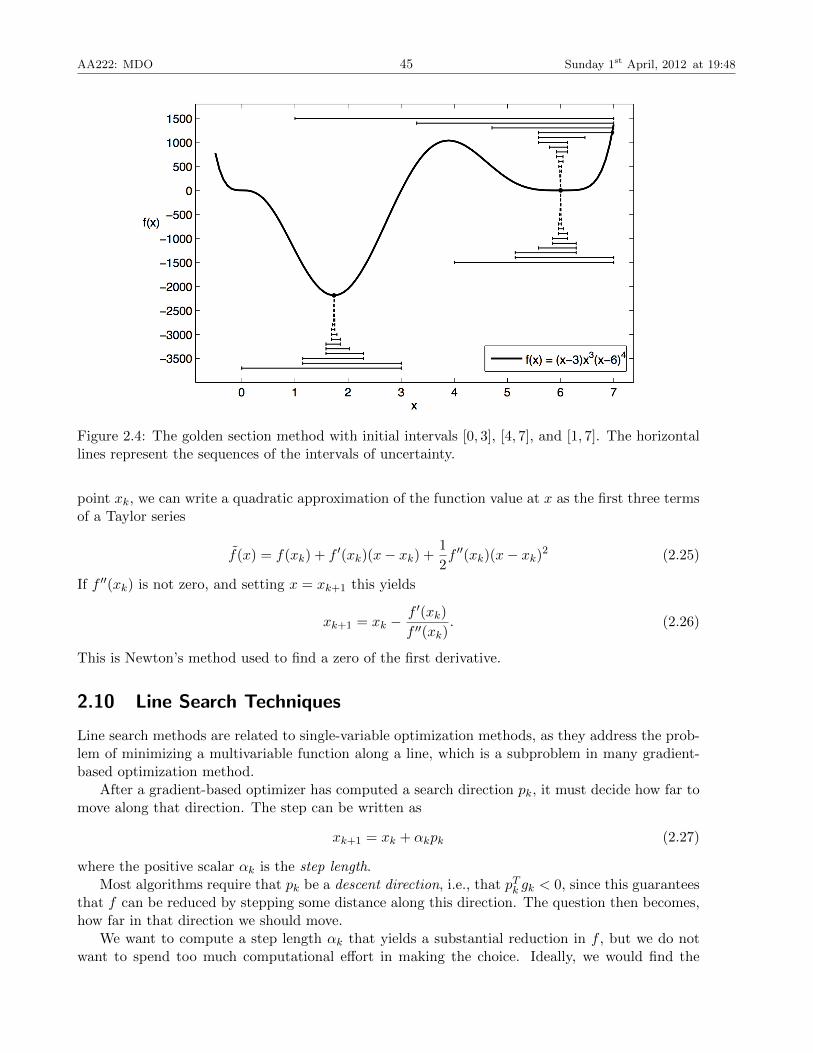
Algorithm 2 Line search algorithm

Input: α1 > 0 and αmax

Output: α∗1: α0 = 02: i← 13: repeat4: Evaluate φ(αi)5: if [φ(αi) > φ(0) + µ1αiφ

′(0)] or [φ(αi) > φ(αi−1) and i > 1] then6: α∗ ← zoom(αi−1, αi)7: return α∗8: end if9: Evaluate φ′(αi)

10: if |φ′(αi)| ≤ −µ2φ′(0) then

11: return α∗ ← αi12: else if φ′(αi) ≥ 0 then13: α∗ ← zoom(αi, αi−1)14: return α∗15: else16: Choose αi+1 such that αi < αi+1 < αmax

17: end if18: i← i+ 119: until

1. the interval between αlow, and αhigh contains step lengths that satisfy the strong Wolfe con-ditions

2. αlow is the one giving the lowest function value

3. αhigh is chosen such that φ′(αlow)(αhigh − αlow) < 0

The interpolation that determines αj should be safeguarded, to ensure that it is not too closeto the endpoints of the interval.

Using an algorithm based on the strong Wolfe conditions (as opposed to the plain Wolfe condi-tions) has the advantage that by decreasing µ2, we can force α to be arbitrarily close to the localminimum.


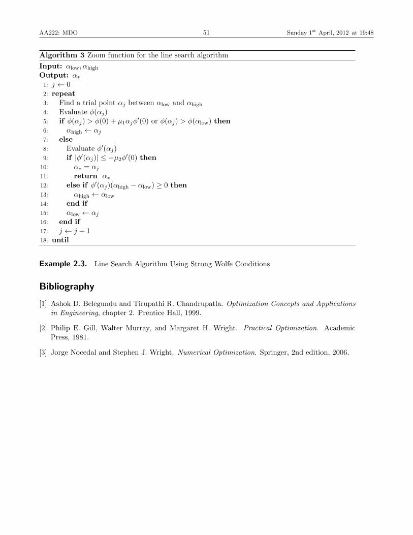
Algorithm 3 Zoom function for the line search algorithm

Input: αlow, αhigh

Output: α∗1: j ← 02: repeat3: Find a trial point αj between αlow and αhigh

4: Evaluate φ(αj)5: if φ(αj) > φ(0) + µ1αjφ

′(0) or φ(αj) > φ(αlow) then6: αhigh ← αj7: else8: Evaluate φ′(αj)9: if |φ′(αj)| ≤ −µ2φ

′(0) then10: α∗ = αj11: return α∗12: else if φ′(αj)(αhigh − αlow) ≥ 0 then13: αhigh ← αlow

14: end if15: αlow ← αj16: end if17: j ← j + 118: until

Example 2.3. Line Search Algorithm Using Strong Wolfe Conditions

Bibliography

[1] Ashok D. Belegundu and Tirupathi R. Chandrupatla. Optimization Concepts and Applicationsin Engineering, chapter 2. Prentice Hall, 1999.

[2] Philip E. Gill, Walter Murray, and Margaret H. Wright. Practical Optimization. AcademicPress, 1981.

[3] Jorge Nocedal and Stephen J. Wright. Numerical Optimization. Springer, 2nd edition, 2006.


Figure 2.8: The line search algorithm iterations. The first stage is marked with square labels andthe zoom stage is marked with circles.

Single Variable Minimization - Stanford...

Documents

Transcript of Single Variable Minimization - Stanford...