Single-Particle Dynamics in Theoretical Minimum Emittance Cell
30
Single-Particle Dynamics in Theoretical Minimum Emittance Cell Yunhai Cai SLAC National Accelerator Laboratory, 2575 Sand Hill Road, Menlo Park, 94205, USA (Dated: September 26, 2018) Abstract We have developed a parameterization of the linear optics in a theoretical minimum emittance cell with three quadrupoles. It consists of five independent parameters: two phase advances, a dimensionless horizontal beta function at the center of the dipole, and a bending angle φ and a length L of the dipole. For the zero chromaticity cell, we again find that the dynamic aperture in the normalized phase space is scaled according to, ¯ A ∝ φ √ L. Moreover, we study nonlinear dynamics near the third-order coupled resonances in the framework of the resonance normal form. In particular, we derive the effective Hamiltonians using the Lie algebra method and show that the periodic orbits in tracking can be interpreted as solutions of the Hamilton’s equations. Surprisingly, we discover that the scheme is not only applicable to the single resonance but also to the double resonances. 1 SLAC-PUB-17346 This material is based upon work supported by the U.S. Department of Energy, Office of Science, under Contract No. DE-AC02-76SF00515.
Transcript of Single-Particle Dynamics in Theoretical Minimum Emittance Cell

Single-Particle Dynamics in Theoretical Minimum Emittance Cell
Yunhai Cai
SLAC National Accelerator Laboratory,
2575 Sand Hill Road, Menlo Park, 94205, USA
(Dated: September 26, 2018)
Abstract
We have developed a parameterization of the linear optics in a theoretical minimum emittance
cell with three quadrupoles. It consists of five independent parameters: two phase advances, a
dimensionless horizontal beta function at the center of the dipole, and a bending angle φ and a
length L of the dipole. For the zero chromaticity cell, we again find that the dynamic aperture
in the normalized phase space is scaled according to, A ∝ φ√L. Moreover, we study nonlinear
dynamics near the third-order coupled resonances in the framework of the resonance normal form.
In particular, we derive the effective Hamiltonians using the Lie algebra method and show that the
periodic orbits in tracking can be interpreted as solutions of the Hamilton’s equations. Surprisingly,
we discover that the scheme is not only applicable to the single resonance but also to the double
resonances.
1
SLAC-PUB-17346
This material is based upon work supported by the U.S. Department of Energy, Office of Science, under Contract No. DE-AC02-76SF00515.
I. INTRODUCTION
Historically, the theoretical minimum emittance (TME) cell [1] has played an essential
role in the advance to a lower emittance in the electron storage rings. Teng illustrated how
the equilibrium emittance is scaled according to the beam energy and deflecting angle of the
dipole and perhaps, most importantly, how it can be minimized to reach its theoretical min-
imum without a specific design of the cell. The optimization scheme was further advanced
by Potier and Rivkin [2, 3] who characterized the cell with a set of the detuned parameters,
namely the ratio to the minimum values, relating them to the horizontal phase advance. The
parameterization laid a solid foundation for a systematic approach [4] to the design of the
low-emittance storage rings [5] and the damping rings [6]. The parameterization provides a
strategical guidance for designing a cell, but it still relies on a computer program to find a
periodic solution of the cell. In this sense, the optimization scheme is not yet complete.
In this paper, we will develop a complete parameterization of the TEM cell that consists of
a dipole magnet, three quadrupoles, and three sextupoles. For simplicity, the sextupoles are
set to make the chromaticity zero. The system is chosen to be a good approximation of the
TME lattice and yet simple enough to be studied analytically. For single-particle dynamics,
we will continue the work of the parameterized FODO cell [7] and explore applications
of the Kolmogorov-Arnold-Moser (KAM) theory [8–11] to particle accelerators. To avoid
repetition, our focus will be placed only on the invariant tori near the nonlinearly coupled
resonances. Mostly, the resonance studies [12–14] were carried out in the framework of the
canonical perturbation theory. Here, our investigation will be from a modern viewpoint of
the Lie Algebra [15] with an emphasis on comparisons to direct tracking.
We will introduce a geometrical parameterization of the focusing system based on the
paraxial optics and apply it to a half cell with a reflection symmetry in section II. Continuing
in section III, we will develop the linear optics, derive the emittance, and then compensate
the chromaticities in the periodic cell. Nonlinear aberrations will be given with a brief
outline in section IV using the Lie Algebra method. Most importantly, we will study the
Hamiltonian dynamics in comparison to the tracking in V and VI sections for one and two
resonances respectively. Finally, in section VII, we will make some concluding remarks. A
solution of the cubic equation and the detailed derivation of the effective Hamiltonian [16]
in a vicinity of resonance and normal form [17] will be given in the Appendix.
2
II. PARAMETERIZATION
A. Paraxial Optics
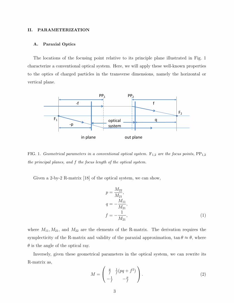
The locations of the focusing point relative to its principle plane illustrated in Fig. 1
characterize a conventional optical system. Here, we will apply these well-known properties
to the optics of charged particles in the transverse dimensions, namely the horizontal or
vertical plane.
in plane out plane
PP2
q
f
F2
PP1
F1
-f
-popticalsystem
FIG. 1. Geometrical parameters in a conventional optical system. F1,2 are the focus points, PP1,2
the principal planes, and f the focus length of the optical system.
Given a 2-by-2 R-matrix [18] of the optical system, we can show,
p =M22
M21
,
q = −M11
M21
,
f = − 1
M21
, (1)
where M11,M21, and M22 are the elements of the R-matrix. The derivation requires the
symplecticity of the R-matrix and validity of the paraxial approximation, tan θ ≈ θ, where
θ is the angle of the optical ray.
Inversely, given these geometrical parameters in the optical system, we can rewrite its
R-matrix as,
M =
qf
1f(pq + f 2)
− 1f
− pf
. (2)
3

B. Doublet
Let us consider a doublet drawn schematically in Fig. 2. Its R-matrix can be obtained
by multiplying the three R-matrices of the elements. Then applying Eq. (1), we have its
geometrical parameters,
-f1f2
g
FIG. 2. A schematic layout of a doublet. f1,2 are focus lengths of the defocusing and focusing
quadrupoles respectively. g is the distance between the quadrupoles.
p =f1(g − f2)
f1 − f2 + g,
q =f2(g + f1)
f1 − f2 + g,
f =f1f2
f1 − f2 + g. (3)
Here we have to use the thin lens calculation for the quadrupoles. Sometimes it is useful
to have its inverse,
f1 = −f2 + pq
f − q,
f2 =f 2 + pq
f + p,
g =f 2 + pq
f. (4)
To focus the charged particles in both transverse planes simultaneously, a doublet is often
required because a magnetic quadrupole focuses in one plane while defocuses in the other.
4

C. A Half Cell
We now consider a half of a cell with a reflection symmetry as shown in Fig. 3, where the
position s1 is the starting and s2 the reflecting points. Here we represent the doublet with
their geometrical parameters, p, q, and f . And L1, L2 are the distances between the doublet
to s1, s2 respectively.
(p,q,f)
s1 s2
L1 L2
FIG. 3. A schematic layout of a half cell for a cell with a reflection symmetry. p, q, and f are the
geometrical parameters of the doublet. L1, L2 are the distances to the entry and exit of the half cell
respectively.
Using the matrix in Eq. (2) for the doublet and the matrix of drift, we compute the
transfer matrix from s1 to s2 and find,
Ms1→s2 =
q−L2
f1f[(p+ L1)(q − L2) + f 2]
− 1f
− (p+L1)f
. (5)
Note that the matrix has the same functional form in Eq. (2) with replacements q → q−L2
and p → p + L1. This property is consistent with the interpretation of the geometrical
parameters, p, q, and f . Also, the matrix can be represented by [19],
Ms1→s2 =
√β2
β1cosπν
√β1β2 sin πν
− 1√β1β2
sin πν√
β1
β2cosπν
, (6)
where β1, β2 are the beta functions [20] at the positions s1, s2 respectively, ν the betatron
tune of the cell. Here we have used the property of the reflection points, namely α1 = α2 = 0.
Comparing it with the matrix in Eq. (5), we obtain,
p = −L1 − β1 cotπν,
q = L2 + β2 cot πν,
f =√β1β2 csc πν. (7)
5

Given these geometrical parameters, the focus lengths of the quadrupoles and separation
distance can be calculated. Substituting Eq. (7) into Eq. (4), we have,
f1 =β1β2 − L1L2 − (L2β1 + L1β2) cotπν
L2 + β2 cotπν −√β1β2 csc πν
,
f2 =L1L2 − β1β2 + (L2β1 + L1β2) cotπν
L1 + β1 cotπν −√β1β2 csc πν
,
g =(β1β2 − L1L2) sinπν − (L2β1 + L1β2) cosπν√
β1β2
. (8)
The formulas in this section are equally applicable to either the horizontal or vertical
plane. In this paper, we choose the horizontal lattice functions to fix the physical parameters
such as the quadrupole strengths since one of our main concerns is the natural emittance, to
which the horizontal tune: ν and the beta function: β2 at the center of the bending dipole
play essential roles [2, 3].
III. PERIODIC CELL
A. Layout
We would like to illustrate how the map works using a periodic TME cell that contains
three quadrupoles as shown in Fig. 4. The cell is chosen because it contains the most essential
ingredients in the common TME cell and yet is analytically solvable. The quadrupoles and
sextupoles are lumped together as a thin multipole with a sector bending dipole in between.
Here ff and fd are the focal lengths of the focusing and de-focusing quadrupoles respectively.
Also φ and L are the bending angle and length of the dipole.
Applying Eq. (8) with a substitution of L1 = 0, L2 = L/2, f1 = 2fd and f2 = ff , we find
the settings of the doublet,
f =
√β1(cotπν − 2β2)
2(√β1 cot πν −
√β2 csc πν)
,
d =β1(2β2 − cotπν)
2(1 + 2β2 cot πν − 2√β1β2 csc πν)
,
g =
√β1(2β2 sin πν − cos πν)
2√β2
, (9)
where d = fd/L, f = ff/L are the dimensionless focusing lengths of the quadrupoles, nor-
malized by the bend length L. Similarly, we use ”bar” to note the scaling of L for the
6

φ
L
ff,κf-fd,-κd ff,κf -fd,-κd
g g
FIG. 4. A periodic theoretical minimum emittance cell with dipole, quadrupole, and sextupole
magnets. φ and L are the bending angle and length of the dipole, ff,d the focus lengths of the
quadrupoles, κf,d the strengths of the sextupoles.
other parameters in the formulas. As we will show later, β1,2 can also be represented by a
function of the betatron tunes. As a result, these dimensionless parameters can be plotted
as a function of the betatron tunes as shown in Fig. 5. The figure shows that higher horizon-
tal tune or smaller emittance is essentially achieved by a combination of stronger focusing
quadrupole and larger separation between the quadrupoles. The larger the spacing between
the quadrupoles in the doublet, the smaller the packing factor of the magnets is. This is a
significant drawback in the TME cell at high tunes.
0.5 0.6 0.7 0.8 0.9 1.0
0.26
0.28
0.30
0.32
νx
f
0.5 0.6 0.7 0.8 0.9 1.0
0.29
0.30
0.31
0.32
0.33
0.34
0.35
0.36
νx
d
0.5 0.6 0.7 0.8 0.9 1.0
0.35
0.40
0.45
0.50
νx
g
FIG. 5. Dimensionless parameters of the doublet as a function of the betatron tunes with various
ratios: νy : νx = 1:4, 1:3, and 1:2 represented by blue, red, and black color respectively.
7
B. Optics
Given the importance of the dipole in generating the natural emittance, we choose the
reference point in the middle of the dipole. The transfer map Mcell of the cell can be
obtained by initializing an identity map and then concatenating it through the maps of
the elements. Here we use the explicit maps of Eqs. (2.5) and (2.6) in reference [21] for
the bends and kicks respectively. The computation is carried out using Mathematica [22].
Taking the Jacobian of the transfer map for the R-matrix and then comparing it with the
Courant-Synder matrix [20] of a periodical system, we find that the betatron tunes, defined
as the phase advances in units of 2π, are given by,
νx = 1− 1
2πcos−12d[f 2 + g − f(2g + 1)] + (f − g)[f(2g + 1)− g]
2df 2,
νy =1
2πcos−12d[f 2 + g + f(2g + 1)]− (f + g)[f(2g + 1) + g]
2df 2. (10)
Moreover, we have the beta functions at the center of the dipole,
βx =[4df − 2d+ f(2g + 1)− g][f(2g + 1)− g]L
4df 2 sin 2πνx,
βy =[4df + 2d− f(2g + 1)− g][f(2g + 1) + g]L
4df 2 sin 2πνy, (11)
and the horizontal dispersion,
ηx =(8df + 4f g − 2d+ f − g)Lφ
8(2d− f + g). (12)
αx,y = 0 and ηpx = 0 due to the reflection symmetry.
C. Emittance
Substituting the physical parameters in Eq. (9) into Eqs. (10, 11, 12) for the optical
functions in the horizontal plane, we obtain,
νx = ν,
βx = β2L,
ηx =1
8Lφ(1 + 4β2 cotπν) (13)
The first two equations are merely a consistency check of the parameterization introduced
in the previous section. The third equation, namely the relationship between the horizontal
8

tune and dispersion, was first derived by Rivkin [3]. Given the beta and dispersion functions,
we evaluate the radiation integrals [23] and derive the form factor,
F =1 + 10β2
2 + 10β2 cotπν + 30β22 cot2 πν
120β2
, (14)
which is defined by the natural emittance εx = CqFγ2φ3 where Cq = 3.8319 × 10⁻¹³m and
γ is the Lorentz factor. It can be minimized and reduced to,
F =1
60(5 cotπν +
√10 + 30 cot2 πν), (15)
by setting,
β2 =1√
10 + 30 cot2 πν. (16)
To minimize the emittance, we alway use this optimal value of β2 in this paper.
0.5 0.6 0.7 0.8 0.9 1.0
0.02
0.03
0.04
0.05
0.06
0.07
0.08
νx
F
FIG. 6. The form factor of emittance in Eq. (15) as a function of the horizontal betatron tune.
As shown in Fig. 6, it can be further minimized by selecting: νmin = 1 − 1π
cot−1√
5/3
with the well-known minimum: [1] Fmin = 1/12√
15. The reduction factor of the emittance
from ν = 0.5 to νmin is about 2.45.
9

D. Linear Stability
Similarly, we can calculate the optical parameters in the vertical plane. In particular, we
find that the betatron tune is given by,
cos 2πνy =1
2β1β2(2β2 sin πν − cosπν)8√β1β2(β1 + 4β2)− β2(47β1 + 16β2) cosπν
+ 8
√β1β2(β1 + 2β2) cos 2πν − 3β1β2 cos 3πν + [30β1β
22 − (β1 + 8β2)] sinπν
+ 2
√β1β2[3− 4(β1β2 + β2
2)] sin 2πν + β1(2β22 − 1) sin 3πν. (17)
This condition has to be satisfied for a stable cell. Essentially, it defines β1 since β2 should
be set according to Eq. (16) for a minimal emittance. In fact, β1 as a function of νx, νy, β2
can be obtained explicitly by solving a cubic equation. The solution is given in Appendix
A. As a result, we have found that five independent parameters, namely νx, νy, β2, φ, L, can
characterize a stable TME cell. It is worth noting that the only dimensional parameter
is the length of the dipole L. The dimensionless horizontal beta functions β1 and β2 as a
function of the betatron tunes are shown in Fig. 7. They depend similarly on the horizontal
tune and hardly any on the vertical tune.
0.5 0.6 0.7 0.8 0.9 1.0
0.00
0.05
0.10
0.15
0.20
0.25
0.30
νx
β1
0.5 0.6 0.7 0.8 0.9 1.0
0.00
0.05
0.10
0.15
0.20
0.25
0.30
νx
β2
FIG. 7. The horizontal beta functions at the end (left) and center (right) of the cell as a function
of the betatron tunes with various ratios: νy : νx = 1:4, 1:3, and 1:2 represented by blue, red, and
black color respectively.
We check the parameterization for the TME cell at the minimum emittance against the
computer program MAD [24]. In particular, the lattice functions computed numerically
using MAD, shown in Fig. 8, excellently agree to the analytical calculations. A drawback of
10

0.0 1.0 2.0 3.0 4.0 5.0 6.0 7.0 8.0 9.0 10.0s (m)
δE/ p0c = 0.0Table name = TWISS
Lattice FunctionsTheoretical Minimum Emittance CellUnix version 8.52/0s 24/09/18 17.11.37
0.0
5.0
10.0
15.0
20.0
25.0
30.0
35.0
40.0
45.0
50.0
β(m
)
0.010
0.015
0.020
0.025
0.030
0.035
0.040
0.045
Dx(m
)
βx βy Dx
FIG. 8. Lattice functions of TME cell at the minimum emittance with νx = νmin, νy = νmin/3,
φ = π/64, and L = 5 m.
the cell is that the vertical beta function at the defocusing quadrupole is too large. As we
will see later, that leads to larger nonlinear aberrations in the vertical plane.
E. Chromatic Compensation
The Courant-Synder parameters with δ dependence can be calculated [21] using the
symplectic maps. In particular, by computing the phase advances up to the first-order of δ,
we derive the natural chromaticity,
ξx0 = − [4df + 3g2 − 4f g(g + 1)− 2df(2g + 1) + f 2(2g + 1)
2π√
(f − g)(2d− f + g)[f(2g + 1)− g + 4df − 2d][f(2g + 1)− g],
ξy0 = − [−4df + 3g2 + 4f g(g + 1)− 2df(2g + 1) + f 2(2g + 1)
2π√
(f + g)(2d− f − g)[f(2g + 1) + g − 4df − 2d][f(2g + 1) + g]. (18)
They are plotted in Fig. 9 as a function of the betatron tunes. The amplitude of horizontal
chromaticity increases rapidly beyond νmin ≈ 0.79. From the viewpoint of the chromaticity
in the vertical plane, the ratio of νy : νx = 1 : 4 or 1 : 3 seems reasonable while 1 : 2 is too
high, largely due to the high vertical beta function at the defocusing quadrupole.
Clearly, we can use the two sextupoles to zero out the natural chromaticity. Solving two
11

0.5 0.6 0.7 0.8 0.9 1.0
-7
-6
-5
-4
-3
-2
-1
0
νx
ξ x0
0.5 0.6 0.7 0.8 0.9 1.0
-4.0
-3.5
-3.0
-2.5
-2.0
-1.5
-1.0
νx
ξ y0
FIG. 9. The natural chromaticity in the horizontal (left) and vertical (right) planes as a function
of the betatron tunes with various ratios: νy : νx = 1:4, 1:3, and 1:2 represented by blue, red, and
black color respectively.
linear equations, we find the necessary strengths,
κf =2(2d− f + g)
(2d+ g)f 2L2φ,
κd =(2d− f − g)
d2fL2φ. (19)
It is worth noting that the settings are identical for the values necessary for the local
0.5 0.6 0.7 0.8 0.9 1.012
14
16
18
20
22
24
26
νx
L2ϕκf
0.5 0.6 0.7 0.8 0.9 1.0
20
22
24
26
28
30
32
34
νx
L2ϕκd
FIG. 10. The settings of focusing (left) and de-focusing (right) sextupoles as a function of the
betatron tunes with various ratios: νy : νx = 1:4, 1:3, and 1:2 represented by blue, red, and black
color respectively.
compensation. As a result, the chromaticities are well corrected. With the formulae, we
plot the strengths of the sextupoles in Fig. 10, which shows that the de-focusing sextupole
is stronger and it can be significantly reduced by lowering the vertical tune.
12

IV. NONLINEARITY
For simplicity, we set the values of the sextupoles at the zero chromaticity in the study
of nonlinear dynamics. It is a good approximation in a single cell because typical circu-
lar accelerators contain many cells and each cell shares only little positive chromaticities.
Moreover, the zero chromaticity reduces the impact of the path lengthening.
Given the settings of the sextupoles in Eq. (19), the third-order Lie polynomial can be
derived similarly to the parameterized FODO cell [7] using the Dragt-Finn factorization [25].
Since the chromaticity is well compensated, the chromatic aberration is negligible. The
geometric part consists of five resonance driving terms and is given by,
f3 =1
φ√L(C2100J
3/2x + C1011J
1/2x Jy) cos(ψx − πνx) + C3000J
3/2x cos 3(ψx − πνx)
+J1/2x Jy[C1020 cos(ψx + 2ψy − πνx − 2πνy) + C1002 cos(ψx − 2ψy − πνx + 2πνy)], (20)
where Jx,y, ψx,y are the action and angle variables [26] in the horizontal and vertical planes
respectively. It should be emphasized that the only dependence on the bending angle φ and
length L of the dipole is in a combination of φ√L in its denominator. This property leads to
the scaling law of the dynamic aperture in the normalized coordinates. Here the coefficients
Cjklm are functions of the remaining parameters: νx,y and β2. Their subscripts indicate the
indices of power series in the complex variables.
0.5 0.6 0.7 0.8 0.9 1.0
0
20
40
60
80
νx
C3000
0.5 0.6 0.7 0.8 0.9 1.0
-80
-60
-40
-20
νx
C1020
FIG. 11. The coefficients of resonance driving terms: 3νx (left) and νx + 2νy (right) as a function
of the betatron tunes with various ratios: νy : νx = 1:4, 1:3, and 1:2 represented by blue, red, and
black color respectively.
13
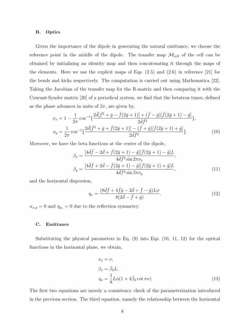
For the horizontal resonances, their coefficients can be written as,
C2100 =1
F[
√β1β2(1 + 8β2
2) cosπνx − β2(1 + 4β1β2 + 4β22 − 2
√β1β2 sin πνx)],
C3000 =1
3F[β2(1− 4β1β2 + 4β2
2) + 2
√β1β2(2β2
2 − 1) cosπνx
+ 2β2(1− 4β22) cos 2πνx −
√β1β2(1− 4β2
2) cos 3πνx
+ 6β2
√β1β2 sin πνx − 8β2
2 sin 2πνx + 4β2
√β1β2 sin 3πνx], (21)
where F = β22
√2β1(2β2 − cot πνx).
Moreover, we obtain the expressions for the three coupled resonances as well. But the
formulas are too lengthy to write out. Here we choose to plot the coefficients of two reso-
nances: 3νx and νx + 2νy in Fig. 11. Their amplitudes are largely following the pattern of
the natural chromaticity in Fig. 9. This finding agrees with an estimate by Levichev and
Kvardakov [27].
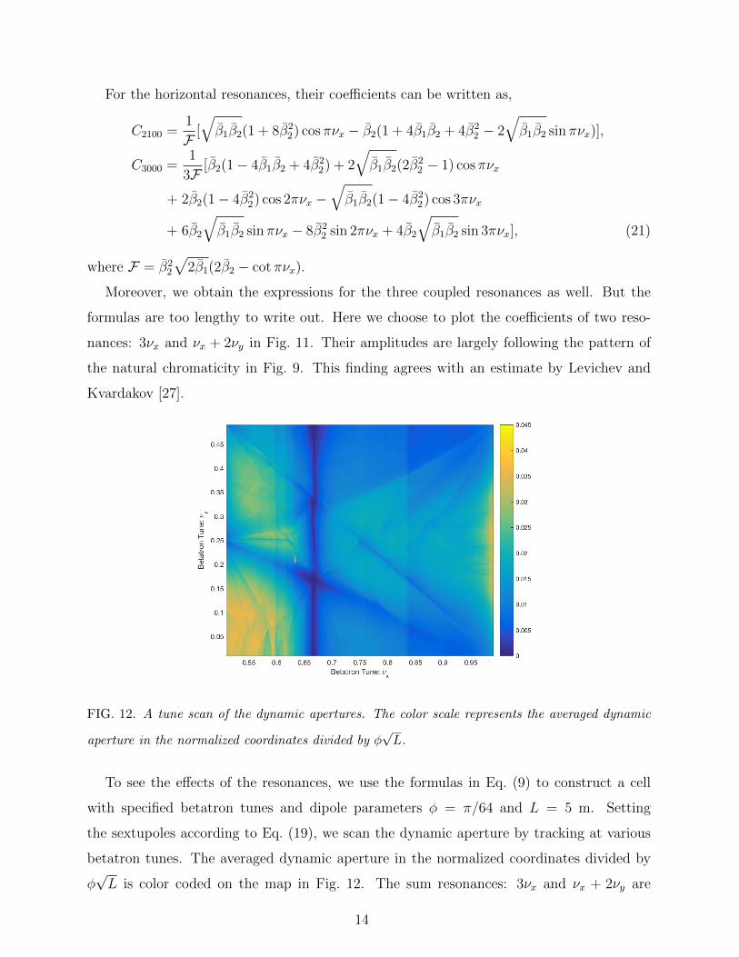
FIG. 12. A tune scan of the dynamic apertures. The color scale represents the averaged dynamic
aperture in the normalized coordinates divided by φ√L.
To see the effects of the resonances, we use the formulas in Eq. (9) to construct a cell
with specified betatron tunes and dipole parameters φ = π/64 and L = 5 m. Setting
the sextupoles according to Eq. (19), we scan the dynamic aperture by tracking at various
betatron tunes. The averaged dynamic aperture in the normalized coordinates divided by
φ√L is color coded on the map in Fig. 12. The sum resonances: 3νx and νx + 2νy are
14

clearly seen and dominant in the tune scan. The dynamic aperture is more than an order
of magnitudes smaller than the one in the parameterized FODO cell [7].
Taking an example of the TME cell with the minimum emittance shown in Fig. 8, 128
cells make an electron storage ring with a circumference of 1210 meter. At an energy of 6
GeV, the natural emittance is 135 pm, which reaches the range of the incoming synchrotron
light sources [28]. Since there are no dispersion-free straights to place the undulators in the
ring, the comparison should be taken only as an estimate. Moreover, the dynamic aperture
at the center of the dipole is 1 mm in the horizontal plane and 2 mm in vertical one, which
is too small for off-axis injection. To increase the dynamic aperture, the phase advances
should be carefully selected for cancellation of the resonance driving terms[4, 29].
V. SINGLE RESONANCE
Near the horizontal resonance 3νx, we obtain similar results as in the study of the pa-
rameterized FODO cell [7]. To avoid repetition, we choose not to write out the finding.
A. Sum Resonance
In the vicinity of the sum resonance: νx+2νy = p+∆ν, where p is an integer, the effective
Hamiltonian can be written as,
H =2π∆ν
5(Jx + 2Jy)−
π∆νC1020
φ√L sin π(p+ ∆ν)
J1/2x Jy cos(ψx + 2ψy). (22)
A derivation will be given in Appendix B. Rewriting the Hamiltonian in terms of the
normalized coordinates, we have,
H =π∆ν
5[(x2 + p2
x) + 2(y2 + p2y)] + θ[x(y2 − p2
y)− 2ypxpy], (23)
where θ is given by,
θ = − π∆νC1020
2φ√
2L sin π(p+ ∆ν). (24)
It is important to know that K = (x2 + p2x)− (y2 + p2
y)/2 is an invariance in this Hamiltonian
system. The invariance can be checked easily by showing that the Poisson bracket of H and
K is zero.
15

1. Invariant Tori
Even with the invariance, the general solution of the Hamilton’s equation is not known.
Here, we would like to find a specific solution,
x = Ax cos(−2µn),
px = −Ax sin(−2µn),
y = Ay cos(µn),
py = −Ay sin(µn), (25)
where n is the turn number as the time variable. Substituting it into the Hamilton’s equation,
we find that it is indeed a solution provided,
4π∆ν + 10Axθ − 5µ = 0,
5A2yθ + 2Ax(π∆ν + 5µ) = 0. (26)
Together with the constant of motion, K = A2x−A2
y/2, we solve these equations and obtain,
Ax =−π∆ν +
√π2∆ν2 + 12Kθ2
6θ,
Ay =1
3
√π2∆ν2 − 12Kθ2 − π∆ν
√π2∆ν2 + 12Kθ2
θ2. (27)
Note that there are other solutions but they are not seen in the tracking.
The solution requires that the condition, π2∆ν2 + 12Kθ2 ≥ 0, is satisfied. Most impor-
tantly, the largest invariant tori is determined by, π2∆ν2 + 12Kθ2 = 0, and we have,
A(max)x = −π∆ν
6θ,
A(max)y =
√2
3|π∆ν
θ|. (28)
The special solution is compared against tracking with the same initial condition in the
vertical plane as shown in Fig. 13. The large amplitudes, the bigger deviation is between
the tracking and analytical solution, indicating strongly the higher order nonlinear effects
in the tracking. The equal increment beyond the largest tori shown in the figure is unstable
in tracking. This is predicted according to the maximal tori in Eq. (28), which is plotted as
the black lines in the figure.
It is worth noting that these invariant tori were first discovered in the Hamiltonian per-
turbation theory by Franchetti and Schmidt [30], who called them “fixed lines” in the 4D
phase space. In fact, they are the periodic orbits.
16

-1 -0.5 0 0.5 1
7x=?p
L #10 -3
-1
-0.5
0
0.5
1
7px=?
pL
#10 -3
-2 -1 0 1 2
7y=?p
L #10 -3
-2
-1
0
1
2
7py=?
pL
#10 -3
-1 -0.5 0 0.5 1
7x=?p
L #10 -3
-2
-1
0
1
2
7y=?
pL
#10 -3
-1 -0.5 0 0.5 1
7px=?p
L #10 -3
-2
-1
0
1
2
7py=?
pL
#10 -3
FIG. 13. A set of invariant tori in the normalized 4D phase spaces near the sum resonance: νx+2νy
with νx = 0.618 and νy = 0.196. The red dots represent the periodic orbits from tracking with bend
length L = 5 m and angle φ = π/64, the blue lines are the special solutions of the Hamiltonian in
Eq. (23) with ∆ν = 0.01 and θ = −76.73 m−1/2, the black lines are the maximal tori predicted by
the theory.
2. Dynamic Aperture
In the design of storage rings, an adequate dynamic aperture is often required. To
compute the dynamic aperture, we track the particles with different amplitudes as shown in
Fig. 14.
Taking a similar approach for the parameterized FODO cell [7], we would like to examine
contours defined by a constant value of the Hamiltonian in Eq. (23) and find a singular
contour. The difference here is that there is another constant of motion K. This allows us
first to solve px with a fixed value of K and substitute it into the Hamiltonian and then
solve py. We find a singularity at,
y =1√2x− π∆ν
2√
2θ. (29)
17

-2 -1.5 -1 -0.5 0 0.5 1 1.5 27x=?
pL #10-3
0
0.5
1
1.5
2
2.5
7y=?p
L
#10-3
trackingtheory: singularitytheory: maximum tori
FIG. 14. Comparison of the dynamic apertures between the theory (blue solid and black dashed
lines) and the tracking (red cross) at a vicinity of the sum resonance: νx + 2νy = 1 + ∆ν with
∆ν = 0.01.
This singularity defines a contour that leads to infinity in the direction of the momentum
py. This line along with an arc with a radius,
√(A
(max)x )2 + (A
(max)y )2 = |π∆ν
2θ|, are plotted
in Fig. 14 for a comparison to the tracking. The theory gives a reasonably good estimate of
the dynamic aperture.
B. Difference Resonance
The effective Hamiltonian near the vicinity of the difference resonance: νx−2νy = p+∆ν,
where p is an integer, can also be derived similarly to the sum resonance and is given by,
H =2π∆ν
5(Jx − 2Jy)−
π∆νC1002
φ√L sin π(p+ ∆ν)
J1/2x Jy cos(ψx − 2ψy). (30)
Here K = (x2 + p2x) + (y2 + p2
y)/2 is the invariance in the Hamiltonian system. Rewriting
the Hamiltonian in the normalized coordinates, we have,
H =π∆ν
5[(x2 + p2
x)− 2(y2 + p2y)] + θ[x(y2 − p2
y) + 2ypxpy], (31)
where θ is given by,
θ = − π∆νC1002
2φ√
2L sin π(p+ ∆ν). (32)
18

1. Invariant Tori
Again, we would like to find a specific solution,
x = Ax cos(2µn),
px = −Ax sin(2µn),
y = Ay cos(µn),
py = −Ay sin(µn). (33)
Note a different sign in the horizontal oscillation in comparison to the sum resonance. Solving
the Hamilton’s equation, along with the constant of motion, K = A2x + A2
y/2, we obtain,
Ax =π∆ν +
√π2∆ν2 + 12Kθ2
6θ,
Ay =1
3
√−π2∆ν2 + 12Kθ2 − π∆ν
√π2∆ν2 + 12Kθ2
θ2. (34)
Unlike the sum resonance, the condition: π2∆ν2+12Kθ2 ≥ 0 is always satisfied and therefore
does not provide any restriction on the stability.
Similarly, the special solution is compared against tracking as shown in Fig. 15. At small
amplitude, we see good agreement between the theory and tracking. As the amplitude grows
large, so does the deviation between the theory and tracking. It strongly reflects the higher
order nonlinear effects.
2. Tune Shifts
It is well known [31] that the most important nonlinear effects in the next order are the
amplitude-dependent tune shifts,
νx(Jx, Jy) = νx + αxxJx + αxyJy,
νy(Jx, Jy) = νy + αxyJx + αyyJx, (35)
where the three coefficients can be computed using the normal form [17] or the Hamiltonian
perturbation theory [26]. As outlined in Appendix C, here we have modified the normal form
to avoid the so-called small denominator near the resonance. For the case being studied,
we numerically evaluate the resonance normal form using differential algebra [32] and find
19

-4 -2 0 2 4
7x=?p
L #10 -3
-4
-2
0
2
4
7px=?p
L
#10 -3
-0.01 -0.005 0 0.005 0.01
7y=?p
L
-0.01
-0.005
0
0.005
0.01
7py=?
pL
-5 0 5
7x=?p
L #10 -3
-0.01
-0.005
0
0.005
0.01
7y=?p
L
-4 -2 0 2 4
7px=?p
L #10 -3
-0.01
-0.005
0
0.005
0.01
7py=?
pL
FIG. 15. A set of invariant tori in the normalized 4D phase spaces near the difference resonance:
νx− 2νy with νx = 0.618 and νy = 0.314. The red dots represent the orbits from tracking with bend
length L = 5 m and angle φ = π/64 and the blue lines are the special solutions of the Hamiltonian
in Eq. (31) with ∆ν = −0.01 and θ = 72.81 m−1/2.
αxx = 1.23× 10³ m−1, αxy = −6.13× 10³ m−1 and αyy = 1.30× 10⁴ m−1. These values are
quite large for a single cell, specially in the vertical plane.
Based on the normal form in Eq. (C8), the effective Hamiltonian in Eq. (31) is a function
of the same nonlinear normalized coordinates as the fourth-order Hamiltonian that generates
the tune shifts. Combining them according to the Cambell-Baker-Hausdorf (CBH) theorem,
we derive the fourth-order effective Hamiltonian,
H =π∆ν
5[(x2 + p2
x)− 2(y2 + p2y)] + θ[x(y2 − p2
y) + 2ypxpy]
+π
4[αxx(x
2 + p2x)
2 + 2αxy(x2 + p2
x)(y2 + p2
y) + αyy(y2 + p2
y)2]. (36)
The solution in Eq. (33) remains a special solution of the Hamilton’s equation with the
following conditions,
π(αxx − 4αxy + 4αyy)A3x − 6θA2
x + 2π[∆ν + (αxy − 2αyy)K]Ax + 2Kθ = 0, (37)
20

-4 -2 0 2 4
7x=?p
L #10 -3
-3
-2
-1
0
1
2
3
7px=?
pL
#10 -3
-0.01 -0.005 0 0.005 0.01
7y=?p
L
-0.01
-0.005
0
0.005
0.01
7py=?p
L-5 0 5
7x=?p
L #10 -3
-0.01
-0.005
0
0.005
0.01
7y=?p
L
-4 -2 0 2 4
7px=?p
L #10 -3
-0.01
-0.005
0
0.005
0.01
7py=?p
L
FIG. 16. A set of invariant tori in the nonlinear normalized 4D phase spaces near the difference
resonance: νx − 2νy with νx = 0.618 and νy = 0.314. The red dots represent the transformed
periodic orbits from tracking and the blue lines are the special solutions of the Hamiltonian in
Eq. (36).
and Ay =√
2(K − A2x). The cubic equation can be solved analytically using the third root:
x2 in Appendix A. The special solution is compared again to the tracking in the nonlinear
normalized coordinates with the same K values as shown in Fig. 16. The displayed orbits
have been transformed to the normalized coordinates by a third-order Taylor map obtained
in the normal form procedure as outlined in Appendix C.
VI. DOUBLE RESONANCES
At the vicinity of two resonances: νx + 2νy = p + ∆ν and 3νx = q + δν, where p, q are
integers, the third-order effective Hamiltonian defined by the three-turn map can be derived
similarly to the sum resonance. First, since the Lie operator associated with the integer p
and q is again an identity , we have
e:−3H0: = e:−π[2δνJx+(3∆ν−δν)Jy ]:, (38)
21
where, H0 = 2π(νxJx + νyJy), is the free Hamiltonian. Secondly, we go through the same
derivation in Appendix B with the replacements, −6π∆ν5J → −π[2δνJx + (3∆ν− δν)Jy] and
µJ → H0. As a result, Eq. (B6) should be replaced by,
−3H = −π[2δνJx + (3∆ν − δν)Jy] +: −π[2δνJx + (3∆ν − δν)Jy] :
(1− e:H0:)f
(r)3 , (39)
where f(r)3 cab be read from Eq. (20),
f(r)3 =
1
φ√L
[C3000J3/2x cos 3(ψx − πνx) + C1020J
1/2x Jy cos(ψx + 2ψy − πνx − 2πνy)]. (40)
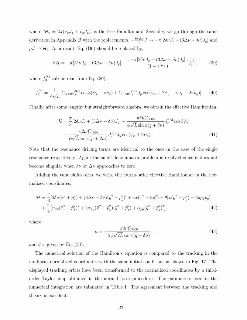
Finally, after some lengthy but straightforward algebra, we obtain the effective Hamiltonian,
H =π
3[2δνJx + (3∆ν − δν)Jy]−
πδνC3000
φ√L sin π(q + δν)
J3/2x cos 3ψx
− π∆νC1020
φ√L sin π(p+ ∆ν)
J1/2x Jy cos(ψx + 2ψy). (41)
Note that the resonance driving terms are identical to the ones in the case of the single
resonance respectively. Again the small denominator problem is resolved since it does not
become singular when δν or ∆ν approaches to zero.
Adding the tune shifts term, we write the fourth-order effective Hamiltonian in the nor-
malized coordinates,
H =π
6[2δν(x2 + p2
x) + (3∆ν − δν)(y2 + p2y)] + κx(x2 − 3p2
x) + θ[x(y2 − p2y)− 2ypxpy]
+π
4[αxx(x
2 + p2x)
2 + 2αxy(x2 + p2
x)(y2 + p2
y) + αyy(y2 + p2
y)2]. (42)
where,
κ = − πδνC3000
2φ√
2L sin π(q + δν), (43)
and θ is given by Eq. (24).
The numerical solution of the Hamilton’s equation is compared to the tracking in the
nonlinear normalized coordinates with the same initial conditions as shown in Fig. 17. The
displayed tracking orbits have been transformed to the normalized coordinates by a third-
order Taylor map obtained in the normal form procedure. The parameters used in the
numerical integration are tabulated in Table I. The agreement between the tracking and
theory is excellent.
22

-5 0 5
7x=?p
L #10 -4
-6
-4
-2
0
2
4
6
7px=?p
L
#10 -4
-2 -1 0 1 2
7y=?p
L #10 -3
-2
-1
0
1
2
7py=?p
L
#10 -3
-6 -4 -2 0 2 4
7x=?p
L #10 -4
-2
-1
0
1
2
7y=?p
L
#10 -3
-6 -4 -2 0 2 4
7px=?p
L #10 -4
-2
-1
0
1
2
7py=?
pL
#10 -3
FIG. 17. A set of invariant tori in the nonlinear normalized 4D phase spaces on the resonance
3νx and near the sum resonance: νx + 2νy with νx = 2/3 and νy = (1/6) + 0.005. The red dots
represent the transformed periodic orbits from tracking and the blue lines are the numerical solution
in Eq. (42).
TABLE I. Parameters for the Double Resonances.
δν ∆ν θ [m−1/2] κ [m−1/2] αxx [m−1] αxy [m−1] αyy [m−1]
0.00 0.01 -90.2402 -22.9766 -6.6074×10² 1.3255×10³ 2.4174×10⁴
VII. CONCLUSION
We have analytically solved the linear optics in a TME cell with three quadrupoles.
The cell can be completely characterized by five independent parameters: its betatron tunes
νx, νy, the dimensionless horizontal beta function at the center of the dipole β2, bending angle
φ, and length L of the dipole. Ideally, β2 should be fixed according to a minimum emittance.
Formulas of the lattice functions, emittance, and natural chromaticity are derived. Three
23

sextupoles in two families are introduced to zero out the chromaticity.
After the chromatic compensation, we derive the complete third-order Lie factor, includ-
ing chromatic and geometric aberrations. The chromatic aberration has been reduced to a
minimum because of the local compensation and hence neglected. The geometric aberration
contains an explicit overall factor of 1/φ√L, leading to a scaling law, A ∝ φ
√L, of the
dynamic aperture in the normalized phase space. We find that the dynamic aperture is
much smaller than that in the FODO cell.
We have studied the third-order coupled resonances in the framework of the resonance
normal form. Near a single sum resonance νx + 2νy, the third-order effective Hamiltonian is
sufficient to explain the dynamics, including the dynamic aperture. It is a strong resonance
resulting in a very small stable region, which is confined by the largest invariant tori.
For the single difference resonance νx − 2νy, again its invariant tori can be described by
the effective Hamiltonian but with the tune-shift terms. More importantly, it is a weak
resonance with a large stable region. The Hamiltonian seems not to define the stability.
Finally, we find that the double resonances 3νx and νx + 2νy can be analyzed similarly to
the single resonance. Its stable region is also similar to the case of the single sum resonance
νx + 2νy.
Our model is greatly simplified in comparison to realistic circular accelerators. Dynamics
of the off-momentum particles can significantly differ from the on-momentum ones. Espe-
cially, we have ignored the high-order terms in energy for the chromaticity or momentum
compaction factor, which can play an important role in full six-dimension tracking with
synchrotron oscillation. To include these effects, the model has to be extended to include a
straight section without any dispersion so that a RF cavity can be placed. A double-bend [33]
or multi-bend [34] achromat could be a good choice for the next investigation.
Acknowledgments
I would like to thank Yuri Nosochkov, Frank Schmidt, Robert Warnock, and Yiton Yan for
helpful discussions. This work was supported by the Department of Energy under Contract
Number: DE-AC02-76SF00515.
24

APPENDIX
Appendix A: Solution of the Cubic Equation
Setting x =√β1, the stability condition in Eq. (17) can be rewritten as a cubic equation,
ax3 + bx2 + cx+ d = 0, (A1)
with the coefficients,
a = −8
√β2(1 + cos 2πν − β2 sin 2πν),
b = 3β2 cos 3πν + β2(47− 2 cos 2πνy) cosπν
+ 2[1− 16β22 + (1− 2β2
2) cos 2πν + 2β22 cos 2πνy] sinπν,
c = 2
√β2[(4β2
2 − 3) sin 2πν − 8β2(2 + cos 2πν)],
d = 8β2(2β2 cosπν + sin πν). (A2)
The solution of the cubic equation is well known. One needs to compute first,
∆0 = b2 − 3ac,
∆1 = 2b2 − 9abc+ 27a2d,
Ω =∆1 +
√∆2
1 − 4∆30
2(A3)
And then the roots are given by,
xk = − 1
3a(b+ ξkΩ1/3 +
∆0
ξkΩ1/3), k ∈ 0, 1, 2, (A4)
where ξ = −12
+ i2
√3. In this paper, we use β1 = x2
0.
Appendix B: Effective Hamiltonian of the Sum Resonance: νx + 2νy
Near the sum resonance, it is well known in the canonical perturbation theory [35] that
J = Jx + 2Jy is the new action and K = 2Jx − Jy is an invariance. Moreover, the free part
of the Hamiltonian can be written as,
−2πνxJx − 2πνyJy = −2π(νx + 2νy)
5J − 2π(2νx − νy)
5K. (B1)
25

Since K is a constant of the motion, the second term can be dropped out from an effective
Hamiltonian. To transfer to the rotating frame, we define the effective Hamiltonian by the
three-turn map,
M3 = e:−3H:. (B2)
This treatment is so obvious as in the case of 3νx [16], seeing a slower variation of the
horizontal betatron phase every three-turn in the tracking. Here, we see a similar pattern
in the tracking of the invariant tori, especially in the vertical plane.
Given µ = 2π(νx + 2νy)/5, we compute the three-turn map,
M3 = (e:−µJ :e:f(r)3 :)3
= e:−3µJ :e:2µJ :e:f(r)3 :e:−2µJ :e:µJ :e:f
(r)3 :e−:µJ :e:f
(r)3 :
= e:−3µJ :e:e:2µJ:f(r)3 :e:e:µJ:f
(r)3 :e:f
(r)3 : (B3)
We start with inserting two identity maps and then apply the similarity transformation
to the Lie operators. Since the Lie operator associated with the integer p is an identity, the
first Lie operator is reduced to,
e:−3µJ : = e:− 6π∆ν5
J :. (B4)
For the next three, we use the CBH theorem for the approximation up to the first order of
f(r)3 and combine them into a single Lie operator,
e:e:2µJ:f(r)3 :e:e:µJ:f
(r)3 :e:f
(r)3 :
≈ e:(e:2µJ:+e:µJ:+1)f(r)3 :
= e:( 1−e:3µJ:
1−e:µJ: )f(r)3 :
= e:( 1−e:
6π∆ν5 J:
1−e:µJ: )f(r)3 :
(B5)
Applying the second form of the CBH theorem to combine two Lie operators in Eqs. (B4)
and (B5) and using the definition of the effective Hamiltonian, M3=e:−3H:, we have,
−3H ≈ −6π∆ν
5J +
: −6π∆ν5J :
(1− e: 6π∆ν5
J :)
(1− e: 6π∆ν5
J :)
(1− e:µJ :)f
(r)3
= −6π∆ν
5J +
: −6π∆ν5J :
(1− e:µJ :)f
(r)3 . (B6)
In addition, the resonance driving term can be read directly from Eq. (20),
f(r)3 =
C1020
φ√LJ1/2x Jy cos(ψx + 2ψy − πνx − 2πνy). (B7)
26
After some straightforward algebra of computing the Poisson brackets, we obtain the Hamil-
tonian,
H =2π∆ν
5(Jx + 2Jy)−
π∆νC1020
φ√L sin π(p+ ∆ν)
J1/2x Jy cos(ψx + 2ψy). (B8)
It is worth noting that it is consistent with the reflection symmetry and more importantly
well behaved as ∆ν approaches zero.
Appendix C: Normal Form in Vicinity of Single Resonance or Double Resonances
We start from the well-known procedure of the normal form [17]. For a nonlinear Taylor
map M truncated at an order o, we make a following transformation,
R−1AMA−1 = I2, (C1)
whereA−1 is a linear map that transforms to the normalized coordinates,R = e:−2π(νxJx+νyJy):
the rotation maps, and I2 is a nonlinear map near the identity. Its lowest perturbation is
the second order, indicated with its subscript.
Similarly, we would like to make a transformation in the next order of perturbation,
e−:N3(z):R−1e:F3(z):AMA−1e−:F3(z): = I3. (C2)
Here we would like to absorb the second-order terms in I2 to F3 and N3. N3 is the driving
term of a single resonance. Inserting an identity map after e:F3:,
e−:N3(z):R−1e:F3(z):RR−1AMA−1e−:F3(z): = I3. (C3)
and using Eq. (C1), and then performing a similarity transformation of the Lie operator
e:F3:, we obtain,
e−:N3(z):e:F3(R−1z):I2e−:F3(z): = I3. (C4)
To solve F3 and N3, we could rewrite this equation as,
e−:N3(z):e:F3(R−1z):e:f(n)3 (z)+f
(r)3 (z):e−:F3(z): = I3, (C5)
where f(n)3 +f
(r)3 is the Lie operator that generates I2 and applying again the CBH theorem,
we obtain
e−:N3(z)+F3(R−1z)+f(n)3 (z)+f
(r)3 (z)−F3(z): = ¯I3. (C6)
27

The solution is given by,
F3(z) = f(n)3 (
1
1−R−1z),
N3(z) = f(r)3 (z). (C7)
It is clear from the solution that N3 has been introduced to absorb all terms that have
1−R−1 near zero value. Once F3 and N3 are calculated, we can compute I3 using Eq. (C4)
and proceed to the next order of perturbation.
This procedure can be continued until the right-hand side becomes identity due to the
order of the truncation of the map. Inverting the Lie operators and maps, we derive the
normal form presentation of the map,
M = A−1e−:F3(~z):...e−:Fo+1(~z):Re:f(r)3 (~z):...e:No+1(~z):e:Fo+1(~z):...e:F3(~z):A. (C8)
[1] L. C. Teng, “Minimizing the Emittance in Designing the Lattice of an Electron Storage Ring,”
Fermilab Report No. TM-1269, 1984.
[2] J. P. Potier and L. Rivkin, “A Low Emittance Lattice for the CLIC Damping Ring,” PAC
Proceedings, p476. Vancouver, B.C. Canada, (1997).
[3] L. Rivkin, in Proceedings of the 7th International Workshop on Linear Colliders (LC97),
Zvenigorod, Russia (INP, Provino, Russia, 1997), p. 644.
[4] P. Emma and T. Raubenheimer, “Systematic Approach to Damping Ring Design,” Phys. Rev.
ST Accel. Beams 4, 021001 (2001).
[5] Y. Jiao, Y. Cai, and A. W. Chao, “Modified Theoretical Minimum Emittance Lattice for an
Electron Storage Ring with Extreme-low Emittance,” Phys. Rev. ST Accel. Beams 14, 054002
(2011).
[6] F. Antoniou and Y. Papaphilippou, “Analytical Considerations for Linear and Nonlinear Op-
timization of the Theoretical Minimum Emittance Cells: Application to the Compact Linear
Collider Predamping Rings,” Phys. Rev. ST Accel. Beams 17, 064002 (2014).
[7] Y. Cai, “Singularity and stability in a periodic system of particle accelerators”, Phys. Rev.
Accel. Beams 21, 054002 (2018).
[8] A. N. Kolmogorov, “On Conservation of Conditionally Periodic Motions of Small Perturbation
of Hamiltonian,” Dokl. Akad. Nauk. SSSR 98 (4), 527 (1954).
28

[9] V. I. Arnold, “Proof of a theorem of A. N. Kolmogokov on the invariance of quasiperoidic
motions under small perturbations of the Hamiltonian,” Usp. Mat. Nauk 18 (5): 13-40 English
translation: Russ. Math. Surv. 18 (5): 9-36 (1963).
[10] J. Moser, “On Invariant Curves of Area-Preserving Mappings on an Annulus,” Nachr. Akad.
Wiss. Gottingem, Math. Phys. K1 2: 1-20 (1962).
[11] A. Morbidelli and A. Giorgilli, “Superexponential Stability of KAM Tori,” Journal of Statis-
tical Physics, Vol. 78, Nos. 5/6, (1995).
[12] R. Hagedorn, “Stability and Amplitude Ranges of Two Dimensional Non-Linear Oscillators
with Periodical Hamiltonian,” CERN 57-1 (1957).
[13] A. Schoch, “Theory of Linear and Non-Linear Perturbations of Betatron Oscillations in Al-
ternating Gradient Synchrotrons,” CERN 57-21 (1958).
[14] G. Guignard, “A General Treatment of Resonances in Accelerators,” CERN 78-11 (1978).
[15] A. J. Dragt, “Lie Algebraic Theory of Geometrical Optics and Optical Aberrations,” J. Opt.
Soc. Am., 72, 372 (1982). A. Dragt et al. “Lie Algebraic Treatment of Linear and Nonlinear
Beam Dynamics”, Ann. Rev. Nucl. Part. Sci., 38, 455 (1988).
[16] A. Chao, “Lecture Notes on Topics in Accelerator Physics,” SLAC-PUB-9574, (2002).
[17] E. Forest, M. Berz, and J. Irwin, “Normal Form Methods for Complicated Periodic Systems:
A Complete Solution Using Differential Algebra and Lie Operators,” Part. Accel. 24 91 (1989).
[18] K. L. Brown, “A First- and Second-Order Matrix Theory for the Design of Beam Transport
Systems and Charged Particle Spectrometers,” SLAC Rep. No 75; Adv. Particle Phys. 1
71-134 (1967).
[19] D. A. Edwards and M. J. Syphers, An Introduction the Physics of High Energy Accelerators,
John Wiley & Sons, Inc., New York (1993).
[20] E. D. Courant and H. S. Snyder, “Theory of the Alternating-Gradient Synchrotron,” Annals
of Physics: 3, 1-48 (1958).
[21] Y. Cai, “Symplectic Maps and Chromatic Optics in Particle Accelerators”, Nucl. Instr. Meth.
A797, p172 (2015).
[22] Mathematica version 9, “A System for Doing Mathematics by Computer,” Wolfram Research.
Inc. (2014).
[23] H. Wiedemann, “Radiation Integrals,” p220 in Handbook of Accelerator Physics and Engi-
neering, Second Edition, Edited by A. Chao, K.H. Mess, M. Tigner, F. Zimmermann, World
29

Scientific, (2013).
[24] H. Grote and F. C. Iselin, “The MAD Program (Methodical Accelerator Design) Version 8.15,”
CERN/SL/90-13 (AP), (1990).
[25] A. J. Dragt and J. M. Finn, “Normal Form for Mirror Machine Hamiltonian, ” J. Math. Phys.
20(12), (1979).
[26] R. D. Ruth, “Single-Particle Dynamics in Circular Accelerator,” AIP Conference Proceedings
No. 153, Vol.1 p150, M. Month and M. Dienes editors (1985).
[27] E. Levichev and V. Kvardakov, “Nonlinear Characteristics of the TME Cell,” RuPAC Pro-
ceedings, p. 327, Novosibirsk, Russia, (2006).
[28] D. Einfeld, “Performance and Perspective of Modern Synchrotron Light Sources,” MOOTH4,
Proceedings of eeFACT2016, Daresbury, UK, (2016).
[29] Y. Cai, “Single-Particle Dynamics in Electron Storage Rings with Extremely Low Emittance,”
Nucl. Instr. Meth. A645, p168 (2011).
[30] G. Franchetti and F. Schmidt, “Extending the Nonlinear-Beam-Dynamics Concept of 1D
Fixed Points to 2D Fixed Lines,” Phys. Rev. Lett. 114, 234801 (2015).
[31] S. Y. Lee, K.Y. Ng, H. Liu, and H. C. Chao, “Evolution of Beam Distribution in Crossing a
Walkinshaw Resonance”, Phys. Rev. Lett. 110, 094801 (2013).
[32] M. Berz, “Differential Algebra Description of Beam Dynamics to Very High Order,” Part.
Accel. 24, 109 (1989).
[33] M. Sommer, “Optimizing of the Emittance Of Electrons (Positrons) Storage Rings”,
LAL/RT/83-15, LAL, November (1983).
[34] D. Einfeld, J. Schaper, and M. Plesko, “A Lattice Design to Reach the Theoretical Minimum
Emittance for a Storage Ring,” p638-640, Proceeding of the 5th European Particle Accelerator
Conference, Barcelona, Spain, Institute of Physics Pub., Bristol, Philadelphia, (1996).
[35] L. Michelotti, “Phase Space Concept,” AIP Conference Proceedings No. 184, Vol.1 p891, M.
Month and M. Dienes editors (1989).
30