Single Organic Molecules and Light Transport in Thin Films
188
I D A M P C XXVIII Coordinatore Prof. Roberto R Single Organic Molecules and Light Transport in Thin Films S S D FIS/ Dottorando Dott. Giacomo M Tutor Dott.ssa Costanza T Coordinatore Prof. Roberto R –
Transcript of Single Organic Molecules and Light Transport in Thin Films

International Doctorate in Atomic and Molecular PhotonicsCiclo XXVIII
Coordinatore Prof. Roberto Righini
Single Organic Molecules and LightTransport in Thin Films
Settore Scientifico Disciplinare FIS/03
DottorandoDott. Giacomo Mazzamuto
TutorDott.ssa Costanza Toninelli
CoordinatoreProf. Roberto Righini
2012–2015


Summary
Two important processes are at the base of light-matter interaction: absorption and scattering.The first part of this work focuses on the interaction of light with single absorbers/emittersembedded in thin films. In the second part, diffusion of light through thin films of scatteringmaterials is numerically investigated.Quantum emitters based on organic fluorescent molecules in thin films are investigated
in the first part of this thesis. The focus of this work is on the experimental characterizationof a specific system consisting of single Dibenzoterrylene (DBT) molecules embedded in athin crystalline matrix of anthracene. The system under investigation exhibits some uniqueoptical properties that enable its use in many applications, especially as a single-photonsource and as a sensitive nanoprobe. In particular, single DBT molecules are very bright andstable within the anthracene matrix. At cryogenic temperatures, dephasing of the moleculardipole due to interactions with the phonons of the matrix vanishes, and as a result the purelyelectronic transition or 00-Zero-Phonon Line becomes extremely narrow, approaching thelimit set by its natural linewidth. Under pulsed excitation, the system can be operated as asource of indistinguishable, lifetime-limited single photons. Furthermore, the spectral shiftsof the narrow ZPL can be exploited as a sensitive probing tool for local effects and fields.In this work we perform a complete optical characterization of the DBT in anthracene
system. Using a home-built scanning epifluorescence microscope, we study its optical prop-erties at room temperature: fluorescence saturation intensity, dipole orientation and emissionpattern, fluorescence and triplet lifetime are investigated. At temperatures down to 3K, weobserve a lifetime-limited absorption line. Also, we demonstrate photon antibunching fromthis system. We then show that single DBT molecules can be effectively used for sensingapplications. Indeed, at the nanometre scale, i.e. on a scale of the order of their physical size,the optical properties of a single molecule are affected by the surrounding environment.In particular, we here demonstrate energy transfer between single DBT molecules and agraphene sheet, a process that can be exploited to measure the distance d between a singlemolecule and the graphene layer. Based on the universality of the energy transfer processand its sole dependence on d, we provide a proof of principle for a nanoscopic ruler.In the second part of this thesis we look at the interaction of light with matter from
a different perspective. By means of numerical simulations, we address the problem oflight transport in turbid media, with a particular focus on optically thin systems. Theproblem is usually modelled by the Radiative Transport Equation and its simple DiffusionApproximation which holds for the case of a single, thick slab of turbid material but failsdramatically for thin systems. Alternatively, the problem of light transport can be modelled
iii

as a random walk process and therefore it can be numerically investigated by means ofMonte Carlo algorithms.
In this work we develop a Monte Carlo software library for light transport in multilayeredscattering samples, introducing several advancements over existing Monte Carlo solutions.We use the software to build a lookup table which allows us to solve the so-called inverseproblem of light transport in a thin slab, i.e. the determination of the microscopic propertiesat the base of light propagation (such as the scattering mean free path ls and the scatteringanisotropy g) starting from macroscopic ensemble observables. We then study diffusionof light in thin slabs, with a particular attention on transverse transport. Indeed, even ifa diffusive behaviour is usually associated with thick, opaque media, as far as in-planepropagation is concerned, transport is unbounded and will eventually become diffusiveprovided that sufficiently long times are considered. By means of Monte Carlo simulations,we characterise this almost two-dimensional asymptotic diffusive regime that sets in evenfor optically thin slabs (OT = 1). We show that geometric and boundary conditions, such asthe refractive index contrast, play an active role in redefining the very asymptotic value ofthe diffusion coefficient by directly modifying the statistical distributions underlying lighttransport in a scattering medium.
iv

Contents
Preface ix
List of publications xv
Acronyms xvii
Symbols xix
I. Organic quantum emitters in thin films 1
1. Quantum light from single emitters 31.1. Different flavours of light . . . . . . . . . . . . . . . . . . . . . . . . . . . . . . 3
1.1.1. Photon statistics . . . . . . . . . . . . . . . . . . . . . . . . . . . . . . . 31.1.2. Second-order correlation function . . . . . . . . . . . . . . . . . . . . 5
1.2. Experimental techniques . . . . . . . . . . . . . . . . . . . . . . . . . . . . . . 71.2.1. Hanbury Brown-Twiss experiment . . . . . . . . . . . . . . . . . . . . 71.2.2. Time-Correlated Single Photon Counting . . . . . . . . . . . . . . . . 9
1.3. Single-photon sources . . . . . . . . . . . . . . . . . . . . . . . . . . . . . . . 101.3.1. Historical notes . . . . . . . . . . . . . . . . . . . . . . . . . . . . . . . 111.3.2. Microscopic single-photon sources in condensed matter . . . . . . . 121.3.3. Applications of single-photon sources . . . . . . . . . . . . . . . . . . 14
2. Single molecules 172.1. Single molecules as sensitive probes and single-photon sources . . . . . . . 172.2. Optical properties of dye molecules in solid matrices . . . . . . . . . . . . . 19
2.2.1. Energy levels and transitions . . . . . . . . . . . . . . . . . . . . . . . 192.2.2. Line shape and homogeneous broadening . . . . . . . . . . . . . . . 222.2.3. Inhomogeneous broadening . . . . . . . . . . . . . . . . . . . . . . . . 24
2.3. Single-molecule detection: fluorescence excitation microscopy . . . . . . . . 252.4. Overview of recent research . . . . . . . . . . . . . . . . . . . . . . . . . . . . 26
3. Spectroscopy and photophysics of single DBT molecules 293.1. DBT in anthracene crystals: an optimal dye-matrix match . . . . . . . . . . . 29
v

Contents
3.2. Methods . . . . . . . . . . . . . . . . . . . . . . . . . . . . . . . . . . . . . . . 313.2.1. Sample preparation . . . . . . . . . . . . . . . . . . . . . . . . . . . . . 313.2.2. Experimental setup . . . . . . . . . . . . . . . . . . . . . . . . . . . . . 343.2.3. Data acquisition and control software . . . . . . . . . . . . . . . . . . 36
3.3. Optical characterization . . . . . . . . . . . . . . . . . . . . . . . . . . . . . . 393.3.1. Photon antibunching . . . . . . . . . . . . . . . . . . . . . . . . . . . . 403.3.2. Saturation behaviour . . . . . . . . . . . . . . . . . . . . . . . . . . . . 413.3.3. Dipole orientation and emission pattern . . . . . . . . . . . . . . . . . 443.3.4. Resonant excitation linewidth at cryogenic temperatures . . . . . . . 473.3.5. Fluorescence lifetime . . . . . . . . . . . . . . . . . . . . . . . . . . . . 483.3.6. Triplet lifetime . . . . . . . . . . . . . . . . . . . . . . . . . . . . . . . 48
3.4. Nano-manipulation of anthracene crystals with AFM . . . . . . . . . . . . . 50
4. Proof of principle for a graphene-based nanoscopic ruler 554.1. Fluorescence near interfaces . . . . . . . . . . . . . . . . . . . . . . . . . . . . 554.2. Graphene: a truly 2D material . . . . . . . . . . . . . . . . . . . . . . . . . . . 564.3. A fundamental nanoscopic ruler by optical means . . . . . . . . . . . . . . . 584.4. A single graphene layer . . . . . . . . . . . . . . . . . . . . . . . . . . . . . . 604.5. Statistical survey of lifetime measurements . . . . . . . . . . . . . . . . . . . 624.6. Discussion . . . . . . . . . . . . . . . . . . . . . . . . . . . . . . . . . . . . . . 644.7. Conclusions . . . . . . . . . . . . . . . . . . . . . . . . . . . . . . . . . . . . . 68
References 69
II. Light transport in thin films 85
5. Theoretical background 875.1. Wave theory of light . . . . . . . . . . . . . . . . . . . . . . . . . . . . . . . . 875.2. Single scattering . . . . . . . . . . . . . . . . . . . . . . . . . . . . . . . . . . . 895.3. Multiple scattering . . . . . . . . . . . . . . . . . . . . . . . . . . . . . . . . . 915.4. The Radiative Transport Equation . . . . . . . . . . . . . . . . . . . . . . . . . 935.5. The Diffusion Approximation . . . . . . . . . . . . . . . . . . . . . . . . . . . 945.6. Diffusion in bounded media . . . . . . . . . . . . . . . . . . . . . . . . . . . . 965.7. Modelling light transport with RandomWalks . . . . . . . . . . . . . . . . . 101
6. MCPlusPlus: a Monte Carlo C++ code for radiative transport 1076.1. Introducing MCPlusPlus . . . . . . . . . . . . . . . . . . . . . . . . . . . . . 1076.2. The Monte Carlo method . . . . . . . . . . . . . . . . . . . . . . . . . . . . . . 1106.3. Software implementation of a random walk for light . . . . . . . . . . . . . . 112
6.3.1. Sample description . . . . . . . . . . . . . . . . . . . . . . . . . . . . . 1136.3.2. Source term . . . . . . . . . . . . . . . . . . . . . . . . . . . . . . . . . 113
vi

Contents
6.3.3. Walker propagation . . . . . . . . . . . . . . . . . . . . . . . . . . . . 1156.3.4. Output . . . . . . . . . . . . . . . . . . . . . . . . . . . . . . . . . . . . 117
7. Deducing effective light transport parameters in optically thin systems 1197.1. Introduction . . . . . . . . . . . . . . . . . . . . . . . . . . . . . . . . . . . . . 1197.2. Methods: simulations and analysis . . . . . . . . . . . . . . . . . . . . . . . . 1227.3. Discussion . . . . . . . . . . . . . . . . . . . . . . . . . . . . . . . . . . . . . . 1247.4. Look-up table approach . . . . . . . . . . . . . . . . . . . . . . . . . . . . . . 1287.5. Conclusions . . . . . . . . . . . . . . . . . . . . . . . . . . . . . . . . . . . . . 133
8. Diffusion of light in thin slabs 1358.1. Introduction . . . . . . . . . . . . . . . . . . . . . . . . . . . . . . . . . . . . . 1358.2. Transport in a thin slab geometry . . . . . . . . . . . . . . . . . . . . . . . . . 1368.3. Methods . . . . . . . . . . . . . . . . . . . . . . . . . . . . . . . . . . . . . . . 1398.4. Discussion . . . . . . . . . . . . . . . . . . . . . . . . . . . . . . . . . . . . . . 1408.5. Conclusions . . . . . . . . . . . . . . . . . . . . . . . . . . . . . . . . . . . . . 143
References 145
III. Attachments 153
Necklace state hallmark in disordered 2D photonic systems 155
Supporting Info: Necklace state hallmark in disordered 2D photonic systems 163
Acknowledgements 167
vii


Preface
This thesis is a handbook of the things I have done and learnt during almost four years ofwork in the Quantum Nanophotonics group at LENS, the European Laboratory for Non-Linear Spectroscopy. Here, I have had the unique opportunity to work both on experimentalactivities as well as on simulations andmodelling, focusing on two diverse aspects regardingthe interaction between light and matter. During this time, I enjoyed intellectual freedom inmy research activity and I had many chances to apply my skills — especially those relatedto software development, of which it seems there is ubiquitous need, both in the laboratoryand for simulation purposes — in the most diverse situations.Two important processes are at the base of light-matter interaction: absorption and scat-
tering. In the first case, probing matter with light allows one to determine its chemicalproperties, since different molecular and atomic species give rise to unique absorptionspectra. Studying how light interacts with matter at the level of a single photon and a singleabsorber/emitter is of fundamental and practical interest. Indeed, strong nonlinear interac-tions are needed for the implementation of schemes for quantum information processingand quantum networks, and they can be obtained already in the few-photon regime from thesaturation of a simple two-level system under efficient excitation. For the class of applica-tions just mentioned, a single-photon source is a fundamental building block. In the secondcase, by studying elastic scattering of a light beam by a turbid medium, information on themicroscopic physical structure of matter can be investigated starting from the observation ofhow light macroscopically spreads in space and time. Besides being of fundamental interest,the study of light transport in particular through thin scattering media has a number ofapplications especially in the field of biomedical optics and diagnostics. In this work, thesetwo aspects of light-matter interaction are covered.
The focus of Part I of this thesis is on the experimental investigation of single-photonsources based on single organic molecules. Such a quantum object produces indeed single-photon states, as described in Chapter 1, where related measurement techniques are alsointroduced. Sources of single, indistinguishable photons are a fundamental building blockfor quantum computation schemes completely relying on linear optics and quantum in-terference effects. While the first single-photon sources were demonstrated with trappedatoms and ions in the gas phase, systems based on emitters in condensed matter — suchas quantum dots, NV centres in diamonds or dye molecules — have recently become moreattractive due to their ease of operation and integration in embedded circuits.
ix

Preface
In Chapter 2 the focus is specifically on (organic) dye molecules embedded in a thin, solidhost matrix. Here we discuss some unique electronic and optical properties emerging insuch configuration. First of all, the crystalline matrix stabilises and protects the organicmolecules from quencher agents such as oxygen, thus strongly preventing photobleaching.Furthermore, when cooled down to cryogenic temperatures, dephasing of the electronicdipole due to interactions with the phonons of the matrix vanishes. Consequently, thepurely electronic Zero-Phonon Line (ZPL) between the first excited state and the groundstate becomes extremely narrow and, for certain host-molecule combinations, it reachesthe limit set by its natural broadening. A lifetime-limited transition is a source of trulyindistinguishable single photons, therefore the system can be employed as a triggered single-photon source, e.g. by means of pulsed excitation. Moreover, the narrow ZPL acts as aresonator with a high quality factor, and as such it can be used to probe very small changesin the nanoenvironment surrounding the molecule. In practice, the frequency shift of theZPL of a single molecule or other effects can be used as extremely sensitive probes for localfields and physical processes occurring at the nanoscale. For all these applications, theisolation and optical detection of a single molecule is a great experimental advancement,often achieved by means of single-molecule fluorescence microscopy.The next chapters are devoted to report the experimental activity in which I took part
in the first two years of this PhD program. In Chapter 3 we propose a specific system ofemitters, consisting of single Dibenzoterrylene (DBT) molecules embedded in thin films ofanthracene, which looks very promising as a single-photon source and for sensing applica-tions. Using a home-built epifluorescence scanning microscope, a complete characterizationof the system’s optical properties was carried out. Several properties were investigated atroom temperature, such as fluorescence saturation intensity, dipole orientation and emis-sion pattern, fluorescence and triplet lifetime. At temperatures down to 3K, we observedlifetime-limited Zero-Phonon Lines. Also, photon antibunching was demonstrated. Theexperimental activity regarding these measurements was particularly challenging and alsoexciting, since the experimental setup had to be built from scratch. In this phase, my maincontribution was the conception and full development of the measurement automation anddata acquisition software — presented in section 3.2.3 — which coordinates the operation ofseveral hardware devices: APDs for fluorescence acquisition, piezo translational stages andgalvo mirrors for sample scanning, a device for Time-Correlated Single Photon Counting(TCSPC), etc. Later, I took part in the measurements and developed some data analysisscripts. Finally, at the Humboldt University in Berlin (Germany) I took part in the explorationof an experimental technique based on combined fluorescence microscopy and Atomic ForceMicroscopy (AFM) aimed at manipulating anthracene crystals on a sub-µm scale.
In Chapter 4we show how our system of single DBT molecules in thin anthracene filmscould be successfully employed as the key ingredient to build a nanosensor. Indeed, at thenanometre scale, i.e. on a scale of the order of their physical size, the optical properties of alight emitter are affected by the surrounding environment. In particular, we demonstrate
x

energy transfer between single DBT molecules and a graphene sheet, a process that can beexploited to measure the distance d between a single molecule and the graphene layer. In ourparticular configuration, DBT molecules close to undoped graphene relax by transferringenergy into the creation of electron-hole pairs in graphene, via a dipole-dipole interactionmechanism similar to Förster Resonance Energy Transfer (FRET). The consequent increase ofthe fluorescence decay rate results in a measurable reduction of the excited state lifetime. Inthis chapter we perform a statistical characterization of the fluorescence lifetimemodificationof single DBT molecules in the presence of graphene. The results are then compared with asimple universal model showing the characteristic d−4 dependence. The simplicity of themodel is such that d appears as the sole unknown, the other parameters being universalquantities. This suggests that the energy transfer mechanism could be used as a nanoruler,i.e. a tool to measure distances at the nanometre scale.In the quest for efficient light-matter interfaces, an experimental effort in our laboratory
is directed towards the coupling of light produced by single DBT molecules with severalkinds of photonic nanostructures or dielectric waveguides. While I did not take part on thisside of the experimental activities, I was instead involved in the numerical study of a specialkind of structures based on thin, disordered 2D photonic crystals. Within such structuresand under certain conditions, localized quasimodes of the electromagnetic field emerge.In some cases coupled modes may appear; these are so-called necklace states. Besides theirfundamental interest, our theoretical investigation was driven by the possibility of exploitingsuch coupled electromagnetic modes to make two remote molecules interact with each other.We performed Finite-Difference Time-Domain simulations of slightly disordered photoniccrystals where the localised quasimodes are excited with point-like dipoles (representingsingle emitters such as single molecules). Since the identification of necklace states in2D is not straightforward, we devised a recipe for their recognition based on the spatialdistribution of the phase of the electromagnetic field. My contribution to this project was inthe development of the analysis software for the calculation of the Fourier transform of thesimulated fields, from which the spatial maps of amplitude and phase that are at the base ofour identification method can be extracted. The task was particularly challenging, given theheavy footprint of the simulations in terms of the size of the output data. I also contributedin the definition of the initial idea of using the phase spatial distribution to assess the natureof localised coupled modes. For the sake of brevity, this work is not presented within themain body of this thesis but the corresponding paper is included in the Attachments part.
Part II of this thesis deals with the numerical investigation of light transport through thinlayers of scattering materials. This was a joint project in which I worked in close cooperationwith dott. Lorenzo Pattelli from the Complex Systems group at LENS. In this study, weinvestigate light transport through turbid media by means of Monte Carlo simulations —using a software package that was entirely developed as part of this thesis — with a specificfocus on optically thin systems.
xi

Preface
In Chapter 5 the theory at the base of the modelling of light transport through a scatteringmedium is introduced. At its core, the Radiative Transport Equation (RTE) simply describesthe energy conservation within a small volume of a scattering material, taking into accountthe losses and gains originating from the scattering process. While simple in its formulation,the RTE cannot be easily solved analytically. In the case of a single, thick slab of turbidmaterial, where a multiple-scattering regime sets in, light transport is very well described interms of the simple Diffusion Approximation, which provides simple analytical formulas forthe most important macroscopic observables (such as the total fraction of transmitted lightand its profile in space and time). However, the approximation fails for optically thin samples,which is a typical case in biomedical optics, since biological materials often naturally comein the form of thin tissues or membranes. Furthermore, no analytical solutions can be foundfor more complicated geometries such as a sample made of multiple layers of differentscattering materials.Given the complexity of a deterministic description of light transport in the multiple-
scattering regime, a solution to the RTE can be found by adopting instead a statisticalapproach in which the scattering process is modelled as a random walk of fictitious, energy-carrying particles. A Monte Carlo method can be used to generate a high number of randomtrajectories within a scattering material and to find an exact solution for the RTE which isonly affected by statistical noise. For the investigations presented in this work, I developeda Monte Carlo software library for light transport in a multilayered system of scatteringmaterials called MCPlusPlus, which is introduced in Chapter 6. This software presentssome significant advantages over existing solutions: it makes possible to access the time-resolved statistics of transmitted light, it comes with an easy-to-use programming interfaceand is capable of efficiently running on modern multi-core computer architectures.In Chapter 7 we tackle the so-called inverse problem of light transport in thin slabs, i.e.
the determination of the microscopic properties at the base of light propagation (such asthe scattering mean free path ls and the scattering anisotropy g) starting from macroscopicensemble observables. This is a problem of primary importance both from the point of viewof fundamental science as well as application-wise, since for example the scattering of lightcan be used as a non-invasive tool to quantitatively measure the properties of in vivo tissues.In our study we simulate light transport through a single thin slab of scattering material byfocusing on two experimental observables. The decay lifetime of the spatially-integratedtransmitted intensity in response to a light pulse impinging on the slab has long beenaccessible experimentally and used used to determine the diffusion properties. Notably, weconsider another robust observable which became experimentally accessible with modernoptical gating techniques, i.e. the Mean Square Width (MSW) growth of the spatial profileof the transmitted pulse. Such quantity grows linearly in time in a diffusive regime, andis inherently robust since by definition it does not depend on absorption and its slope isdirectly related to the diffusion coefficient. In our study we build a large database of thesetwo observables over a broad parameter space in terms of ls, g and optical thickness (ranging
xii
from 1 to 10). With the combined use of these two macroscopic quantities, which are bothexperimentally accessible, we develop a look-up table routine that allows us to retrieve themicroscopic transport properties such as ls and g in the relevant case of a thin slab.
In Chapter 8 we study diffusion of light in thin slabs with a particular focus on transversetransport. Light diffusion is usually associated with thick, opaque media. Indeed, multiplescattering is necessary for the onset of the diffusive regime and such condition is generallynot met in almost transparent media. However, as far as in-plane propagation is concerned,transport is unbounded and will eventually become diffusive provided that sufficientlylong times are considered. By means of Monte Carlo simulations, we characterise thisalmost two-dimensional asymptotic diffusive regime that sets in even for optically thin slabs(OT = 1). We again make extensive use of the MSW growth in time, since this observable isrelated to transverse propagation. Even at such low optical thickness, we find a signatureof diffusive behaviour in the linear increase of the MSW slope with time, which howeverobviously deviates from the prediction cast by the Diffusion Approximation. We show thatgeometric and boundary conditions, such as the refractive index contrast, play an active rolein redefining the very asymptotic value of the diffusion coefficient by directly modifying thestatistical distributions underlying light transport in a scattering medium.
Sesto Fiorentino, 27th November 2015
xiii


List of publications
• G. Mazzamuto, A. Tabani, S. Pazzagli, S. Rizvi, A. Reserbat-Plantey, K. Schädler, G.Navickaite, L. Gaudreau, F. Cataliotti, F. Koppens, and C. Toninelli. “Single-moleculestudy for a graphene-based nano-position sensor”. In: New Journal of Physics 16, 11(2014), p. 113007.
• G. Mazzamuto, A. Tabani, S. Pazzagli, S. Rizvi, A. Reserbat-Plantey, K. Schädler, G.Navickaite, L. Gaudreau, F. Cataliotti, F. Koppens, and C. Toninelli. “Coupling ofsingle DBT molecules to a graphene monolayer: proof of principle for a graphenenanoruler”. In: MRS Proceedings. Cambridge University Press. 2015, p. 1728.
• G. Mazzamuto, L. Pattelli, D. Wiersma, and C. Toninelli. Deducing effective light trans-port parameters in optically thin systems. Sept. 2015.arXiv: 1509.04027 [physics.optics]. Accepted for publication in NJP.
• L. Pattelli, G. Mazzamuto, C. Toninelli, and D. Wiersma. Diffusion of light in semitrans-parent media. Sept. 2015.arXiv: 1509.04030 [physics.optics]
• G. Mazzamuto. Sistema di acquisizione dati e controllo per misure su singole molecole contecniche di microscopia di fluorescenza. National Instruments case study.url: http://sine.ni.com/cs/app/doc/p/id/cs-15965
• G. Kewes, M. Schoengen, G. Mazzamuto, O. Neitzke, R.-S. Schönfeld, A. W. Schell,J. Probst, J. Wolters, B. Löchel, C. Toninelli, and O. Benson. Key components for nano-assembled plasmon-excited single molecule non-linear devices. Jan. 2015.arXiv: 1501.04788 [physics.optics]
• F. Sgrignuoli, G. Mazzamuto, N. Caselli, F. Intonti, F. S. Cataliotti, M. Gurioli, andC. Toninelli. “Necklace state hallmark in disordered 2D photonic systems”. In: ACSPhotonics 2, 11 (2015), pp. 1636–1643. Full text attached on page 155.
xv


Acronyms
AFM Atomic Force Microscopy.APD Avalanche Photo Diode.
BFP Back Focal Plane.
CCD Charge-Coupled Device.CQED Cavity Quantum Electrodynamics.CW Continuous-Wave.
DA Diffusion Approximation.DAQ Data Acquisition.DBATT Dibenzanthanthrene.DBT Dibenzoterrylene.DBT:anth DBT molecules embedded in thin anthracene crystals.DE Diffusion Equation.DFB Distributed FeedBack.DT Diffusion Theory.
EBC Extrapolated Boundary Condition.ECDL External Cavity Diode Laser.
FRET Förster Resonance Energy Transfer.
HBT Hanbury Brown – Twiss.HOMO Highest Occupied Molecular Orbital.
IC Internal Conversion.IRF Instrument Response Function.ISC Inter System Crossing.
LUMO Lowest Unoccupied Molecular Orbital.LUT Look-Up Table.
xvii

Acronyms
MC Monte Carlo.MSW Mean Square Width.
NA Numerical Aperture.
OT Optical Thickness.
PAH Polycyclic Aromatic Hydrocarbons.PDF Probability Density Function.PMMA poly(metyl methacrylate).PRNG Pseudo-Random Number Generator.PS poly(styrene).PSB Phonon Side Band.PVA poly(vinyl alcohol).
QD Quantum Dot.QIP Quantum Information Processing.QY Quantum Yield.
RNG Random Number Generator.RPM Revolutions Per Minute.RTE Radiative Transport Equation.RTT Radiative Transport Theory.
SEM Scanning Electron Microscope.SLD Step Length Distribution.SLOC Single Lines Of Code.SMS Single Molecule Spectroscopy.SNR Signal-to-Noise Ratio.SPAD Single Photon Avalanche Diode.
TCSPC Time-Correlated Single Photon Counting.Ti:sa Titanium-Sapphire.TLS Two-Level System.TTL Transistor-Transistor Logic.TTTR Time-Tagged–Time-Resolved.
ZBC Zero Boundary Condition.ZPL Zero-Phonon Line.
xviii

Symbols
|S0〉 electronic ground state (singlet).|S1〉 first electronic excited state (singlet).|T1〉 first electronic excited state (triplet).
a† creation operator.a annihilation operator.αDW Debye-Waller Factor.αFC Frank-Condon Factor.
D diffusion coefficient.DDA diffusion coefficient as predicted by the Diffusion Approximation (DA).∆νhom homogeneous linewidth.∆νnat natural linewidth.
φF fluorescence quantum yield.
g anisotropy factor.g(2) second-order correlation function.Γ0 decay rate in free space.γhom homogeneous linewidth.γnat homogeneous linewidth.Γ2 total dephasing rate of the |S1〉 → |S0〉 coherence.Γg decay rate of an emitter on top of a graphene monolayer.Γng decay rate in the reference case, i.e. without graphene.Γnrad decay rate for non-radiative emission.Γrad decay rate for radiative emission.
h Planck constant, 6.626 070 040× 10−34 J s.
I(r, t, s) radiance or specific intensity.IS saturation intensity.
k21 rate of direct decay from |S1,ν=0〉 to |S0,ν=0〉.
xix

Symbols
kB Boltzmann constant.kISC Inter System Crossing rate.kT total decay rate from the lowest triplet state.
Leff effective thickness.la absorption mean free path.ls scattering mean free path.lt transport mean free path.
µa absorption rate.µe extinction coefficient.µ′s reduced scattering coefficient.
n refractive index or refractive index contrast, photon number.NA Avogadro constant.n photon number operator.
p(s, s′) scattering phase function.p(l) Step Length Distribution.
σp absorption cross section.
T1 population decay time of the |S1〉 → |S0〉 transition.T2 total dephasing time of the |S1〉 → |S0〉 coherence.T∗2 pure dephasing time of the |S1〉 → |S0〉 coherence.τ decay lifetime, time lag in correlation measurements.τDA decay lifetime as predicted by the Diffusion Approximation (DA).τF fluorescence lifetime.τnrad non-radiative decay lifetime.τrad radiative decay lifetime.
Ud(r, t) average diffuse intensity.
w2(t) Mean Square Width of a transmitted profile.
ze extrapolated length.
xx
Part I.
Organic quantum emitters in thinfilms


Chapter 1.
Quantum light from single emitters
In this chapter we provide a broad introduction on single quantum emitters and their impact onsingle-photon sources. We start by laying out some fundamental concepts that are specific to thephysics of individual quantum objects and that will be later used in the rest of this work. Weshall first recall the quantum properties of light produced by single emitters by introducing threeclassifications of light based on the photon statistics and on the photon distribution in time. Inparticular, the concepts of sub-Poissonian and antibunched light are introduced. We then reviewsome experimental techniques that can be used to assess the quantum nature of light and to measureother time-resolved processes, such as the excitation and relaxation dynamics of a quantum emitter:the Hanbury Brown – Twiss (HBT) experiment and the Time-Correlated Single Photon Counting(TCSPC) technique. Finally, an overview on single-photon sources and their applications is given,with a greater emphasis on condensed matter systems.
1.1. Different flavours of light
1.1.1. Photon statistics
Light emitted by a single quantum source exhibits unique properties that can be used in anumber of applications. In this section we will briefly discuss how different classificationsof light can be made in terms of photon statistics and in terms of how photons are spaced intime in a light beam.
As a reference case, let’s consider a perfectly coherent light beam:
E(x, t) = E0 sin(kx−ωt + φ) (1.1)
where E(x, t) is the electric field module of the light wave and where the angular frequencyω and phase φ are constant in time. The beam intensity I is proportional to the square of theamplitude and is constant since we have assumed ω and φ independent of time. A perfectlycoherent light of constant intensity in the classical sense exhibits, from the point of view ofits fundamental constituents, Poissonian photon statistics, i.e. the distribution of the photonnumber n is given by [1]:
P(n) = nn!
e−n n ∈N (1.2)
Poisson statistics generally describes processes that are intrinsically random, such as thenumber of counts registered by a Geiger counter in front of a radioactive source. In this case,
3

Chapter 1. Quantum light from single emitters
60 80 100 120 140
0
2
4
6
8
·10−2
sub-Poissonian
Poissonsuper-Poissonian
n = 100
n
P(n)
(a)
0 5 10 15 20
0
0.5
1
1.5
2
τ
g(2)(τ)
bunchedcoherent (random)antibunched
(b)
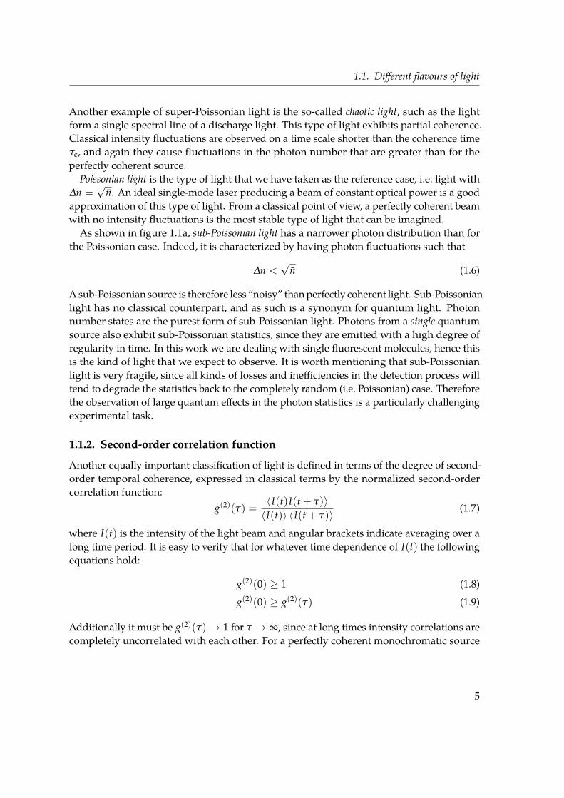
Figure 1.1.: (a) Comparison of the photon statistics for Poissonian, super-Poissonian and sub-Poissonian light. All the distributions shown have an average photon number of n = 100; being n sohigh, the discrete nature of the distributions cannot be appreciated. (b) Second-order correlationfunction g(2)(τ) for bunched, perfectly coherent and antibunched light. The inset shows how photonsare spaced out in the photon stream for the three cases.
the observed counts fluctuate around the average value n because of the random nature ofthe decay process. A similar distribution applies to the count rate registered by a photon-counting device able to detect individual photons in a light beam of constant intensity asthe one considered above. Here the randomness is due to the discrete nature of photons,with an equal probability of finding a photon within any given time interval. A Poissondistribution is only characterized by the mean value n and its standard deviation is given by
∆n =√
n (1.3)
With respect to the reference case described above, we define three types of light basedon their standard deviation of their photon number distribution (see figure 1.1a) which arebriefly described below.Super-Poissonian light is defined by the relation:
∆n >√
n (1.4)
Light following a super-Poissonian distribution is the most frequently found, since allclassical forms of light showing intensity fluctuations in time are expected to exhibit largerphoton number fluctuations than for the case with a constant intensity. Thermal light orblack-body radiation is indeed a notable example of super-Poissonian light. In this case, thephoton statistics of a single mode of the radiation field is the Bose-Einstein distribution:
Pω(n) =1
n + 1
(n
n + 1
)n
(1.5)
4
1.1. Different flavours of light
Another example of super-Poissonian light is the so-called chaotic light, such as the lightform a single spectral line of a discharge light. This type of light exhibits partial coherence.Classical intensity fluctuations are observed on a time scale shorter than the coherence timeτc, and again they cause fluctuations in the photon number that are greater than for theperfectly coherent source.
Poissonian light is the type of light that we have taken as the reference case, i.e. light with∆n =
√n. An ideal single-mode laser producing a beam of constant optical power is a good
approximation of this type of light. From a classical point of view, a perfectly coherent beamwith no intensity fluctuations is the most stable type of light that can be imagined.
As shown in figure 1.1a, sub-Poissonian light has a narrower photon distribution than forthe Poissonian case. Indeed, it is characterized by having photon fluctuations such that
∆n <√
n (1.6)
A sub-Poissonian source is therefore less “noisy” thanperfectly coherent light. Sub-Poissonianlight has no classical counterpart, and as such is a synonym for quantum light. Photonnumber states are the purest form of sub-Poissonian light. Photons from a single quantumsource also exhibit sub-Poissonian statistics, since they are emitted with a high degree ofregularity in time. In this work we are dealing with single fluorescent molecules, hence thisis the kind of light that we expect to observe. It is worth mentioning that sub-Poissonianlight is very fragile, since all kinds of losses and inefficiencies in the detection process willtend to degrade the statistics back to the completely random (i.e. Poissonian) case. Thereforethe observation of large quantum effects in the photon statistics is a particularly challengingexperimental task.
1.1.2. Second-order correlation function
Another equally important classification of light is defined in terms of the degree of second-order temporal coherence, expressed in classical terms by the normalized second-ordercorrelation function:
g(2)(τ) =〈I(t)I(t + τ)〉〈I(t)〉 〈I(t + τ)〉 (1.7)
where I(t) is the intensity of the light beam and angular brackets indicate averaging over along time period. It is easy to verify that for whatever time dependence of I(t) the followingequations hold:
g(2)(0) ≥ 1 (1.8)
g(2)(0) ≥ g(2)(τ) (1.9)
Additionally it must be g(2)(τ)→ 1 for τ → ∞, since at long times intensity correlations arecompletely uncorrelated with each other. For a perfectly coherent monochromatic source
5
Chapter 1. Quantum light from single emitters
photons1 4
3
2 D4
D3
startstop
counter/timer
(a)
CFD
start
CFD ∆t
stopTAC ADC
memory
(b)
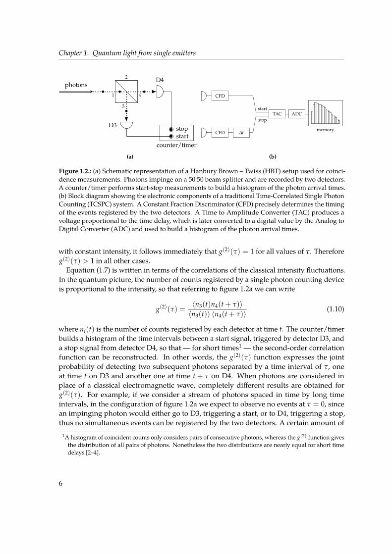
Figure 1.2.: (a) Schematic representation of a Hanbury Brown – Twiss (HBT) setup used for coinci-dence measurements. Photons impinge on a 50:50 beam splitter and are recorded by two detectors.A counter/timer performs start-stop measurements to build a histogram of the photon arrival times.(b) Block diagram showing the electronic components of a traditional Time-Correlated Single PhotonCounting (TCSPC) system. A Constant Fraction Discriminator (CFD) precisely determines the timingof the events registered by the two detectors. A Time to Amplitude Converter (TAC) produces avoltage proportional to the time delay, which is later converted to a digital value by the Analog toDigital Converter (ADC) and used to build a histogram of the photon arrival times.
with constant intensity, it follows immediately that g(2)(τ) = 1 for all values of τ. Thereforeg(2)(τ) > 1 in all other cases.Equation (1.7) is written in terms of the correlations of the classical intensity fluctuations.
In the quantum picture, the number of counts registered by a single photon counting deviceis proportional to the intensity, so that referring to figure 1.2a we can write
g(2)(τ) =〈n3(t)n4(t + τ)〉〈n3(t)〉 〈n4(t + τ)〉 (1.10)
where ni(t) is the number of counts registered by each detector at time t. The counter/timerbuilds a histogram of the time intervals between a start signal, triggered by detector D3, anda stop signal from detector D4, so that — for short times1 — the second-order correlationfunction can be reconstructed. In other words, the g(2)(τ) function expresses the jointprobability of detecting two subsequent photons separated by a time interval of τ, oneat time t on D3 and another one at time t + τ on D4. When photons are considered inplace of a classical electromagnetic wave, completely different results are obtained forg(2)(τ). For example, if we consider a stream of photons spaced in time by long timeintervals, in the configuration of figure 1.2a we expect to observe no events at τ = 0, sincean impinging photon would either go to D3, triggering a start, or to D4, triggering a stop,thus no simultaneous events can be registered by the two detectors. A certain amount of1A histogram of coincident counts only considers pairs of consecutive photons, whereas the g(2) function givesthe distribution of all pairs of photons. Nonetheless the two distributions are nearly equal for short timedelays [2–4].
6

1.2. Experimental techniques
time has to be waited for a second photon to trigger a stop pulse, therefore detected eventsare expected to increase in time. This clearly violates equations (1.8) and (1.9) for classicalfields. If instead we consider a stream of photons arriving in bunches, simultaneous countsfrom the two detectors are highly probable, with a large number of events registered nearτ = 0 and fewer at longer delays, since the probability of detecting a stop photon after astart one has been registered decreases with time. This picture is in perfect agreement witha classical framework. Again, since we have found different behaviours for light which canhave a classical counterpart or be purely quantum, we make another threefold distinctionbased on the second-order correlation function g(2)(τ).Bunched light occurs when g(2)(0) > g(2)(τ), i.e. when photons arrive grouped together
in bunches. Therefore, if a photon is detected at t = 0, there’s a higher probability to detectanother photon at short times rather than at long delays. From equations (1.8) and (1.9), itfollows that classical light is bunched, as is chaotic light from a discharge lamp.As already anticipated, perfectly coherent light has g(2)(τ) = 1. Indeed, since it is charac-
terized by Poissonian photon statistics, photons are randomly spaced in time. Therefore,once a photon is detected, the probability to detect another photon is the same for all valuesof τ. Coherent light is compatible with a classical picture, since it satisfies equations (1.8)and (1.9).Antibunched light is a pure quantum phenomenon, having
g(2)(0) < g(2)(τ) (1.11)
which violates equation (1.9). In antibunched light, photons tend to arrive evenly spaced intime, rather than with random spacing. The regularity with which photon arrives meansthat there will be relatively long time delays between successive photons, i.e. a lower proba-bility of observing counts at short delays. Photon antibunching is usually, but not always2,accompanied by sub-Poissonian photon statistics, in which case g(2)(0) < 1.
1.2. Experimental techniques
1.2.1. Hanbury Brown-Twiss experiment
The experimental configuration of figure 1.2a is commonly known as Hanbury Brown –Twiss (HBT) arrangement, after the two scientists who first used this setup while studyingthe coherence properties of astrophysical sources [7]. The setup consists of a 50:50 beamsplitter, which equally divides incident photons between the two output ports. The photonsthen impinge on two single-photon counting Avalanche Photo Diodes (APDs). Every timethey detect a photon, the APDs produce a pulse which is fed into an electronic counter/timer
2Antibunched light does not necessarily exhibit sub-Poissonian statistics [5]. Additionally, a two-mode statecan be constructed in which the counting statistics are sub-Poissonian, while photons exhibit bunching intime [6].
7

Chapter 1. Quantum light from single emitters
which we will better describe in section 1.2.2. This electronic device records the time delaysbetween pulses from detectors D3 and D4, and builds a histogram of the registered delayswhich approximates the g(2) function at short times. A HBT experiment allows to observephoton antibunching, therefore it makes it possible to assess the quantum nature of light.In a typical antibunching measurement, a single emitting species (such as an individualatom, molecule, quantum dot or colour centre) is excited using laser radiation and itsfluorescence is collected by detectors arranged in the HBT configuration. Once a photonis emitted, a subsequent photon can only be emitted following another excitation cycle, i.e.on average after an amount of time approximately equal to the radiative lifetime of thetransition. Since the photons arrive at the detectors with long gaps in between them, this willresult in the observation of the typical dip associated with antibunched light (figure 1.1b).Photon antibunching was first successively observed by Kimble et al. in 1977 in resonancefluorescence experiments with sodium atoms [8]. As far as single molecules are concerned,the first experimental evidence of photon antibunching was found in 1992 by Basché et al.with single pentacene molecules embedded in a p-terphenyl crystal at 1.5K [9].
In section 1.1.2 we highlighted how the second-order correlation function classically de-scribes intensity correlations, whereas in a quantum picture it depends on the simultaneousprobability of counting photons at time t on D3 and at time t + τ on D4. For a quantumanalysis of the HBT experiment, we can rewrite equation (1.10) as [1]:
g(2)(τ) =⟨
a†3(t)a†
4(t + τ)a4(t + τ)a3(t)⟩
⟨a†
3(t)a3(t)⟩ ⟨
a†4(t + τ)a4(t + τ)
⟩ (1.12)
where we have used the photon number operator n = a† a. We are particularly interested inthe value for g(2)(0), since this gives a clear evidence of quantum behaviour:
g(2)(0) =⟨
a†3 a†
4 a4 a3⟩
⟨a†
3 a3⟩ ⟨
a†4 a4⟩ (1.13)
The expressions for the annihilation operators for the output ports are:
a3 = (a1 − a2)/√
2
a4 = (a1 + a2)/√
2(1.14)
and the corresponding creation operators are found by taking the Hermitian conjugates. Ina HBT experiment, photons impinge only on input port 1, so that the vacuum state has to beconsidered at port 2. The input state is therefore written as:
|Ψ〉 = |ψ1, 02〉 (1.15)
where ψ1 is the input state at port 1 and 02 is the vacuum state at port 2. Having the vacuumstate at one port greatly simplifies the final expression, which after some easy calculationscan be written as:
g(2)(0) =〈ψ1|n1(n1 − 1)|ψ1〉/4
(〈ψ1|n1|ψ1〉/2)2 (1.16)
8

1.2. Experimental techniques
If the input state is the photon number state |n〉, then we obtain:
g(2)(0) =n(n− 1)
n2 = 1− 1n
(1.17)
Therefore, for a single-photon source, i.e. a source emitting photon number states with n = 1,we expect to obtain the highly non-classical result of g(2)(0) = 0 from a HBT measurement.
1.2.2. Time-Correlated Single Photon Counting
The relaxation dynamics of an emitter following an excitation event can be investigated bymeans of time-resolved detection of the emitted photons. Time-Correlated Single PhotonCounting (TCSPC) is a well established and common technique for fluorescence lifetimemeasurements [10, 11], but it can also be used for photon coincidence correlation measure-ments in a HBT setup to observe antibunching effects. The method consists in the accurateregistration of the arrival times of single photons relative to a reference signal. By periodicexcitation, e.g. from a pulsed laser source, the fluorescence decay profile is reconstructedover multiple excitation cycles.A detector, typically a Single Photon Avalanche Diode (SPAD), generates a pulse per
each detected photon with very accurate timing of the photon arrival (typical timing jitter≈ 100 ps). The pulse is then fed to the TCSPC electronics, which globally operate as a stop-watch. Figure 1.2b shows a block diagram of a traditional TCSPC system. In a fluorescencespectroscopy laboratory, it was not uncommon to implement a TCSPC system by chainingtogether the single standalone blocks shown in the figure. Today, more modern and compactcommercial solutions exist, which embed sophisticated electronics in a single device. This isthe case for example of the PicoHarp module by PicoQuant, which we have used for allthe TCSPC measurements in this work. The first block in the electronic chain is a ConstantFraction Discriminator (CFD). It is used to extract the precise timing of pulses which mayvary in amplitude, which is typical when the detectors used are Photomultiplier Tubes(PMT) or Microchannel Plates (MCP). In addition to the detector signal, the reference orsync signal is a required input for the electronics. Both signals are directed to a Time toAmplitude Converter (TAC), which is basically a highly linear integrator. The sync signaltriggers the start of a ramp generator, which is later stopped by the signal coming from thedetector. Therefore, the resulting signal at the TAC output is a voltage proportional to thetime lag between the two inputs. The voltage produced by the TAC is digitized by an Analogto Digital Converter (ADC) and used to address the corresponding bin in the histogram ofarrival times. In time-resolved fluorescence measurements, the reconstructed histogramshows an exponential drop of counts at later times.
The configuration described above is called forward mode, in which the periodic excitationsource provides the sync signal and the detected fluorescence photon provides the stopsignal. However, the repetition rate of the excitation laser is much higher than the rate ofdetected photons, since not all the excitation pulses cause a photon event. Therefore, when
9

Chapter 1. Quantum light from single emitters
working in this mode, the TAC overflows and has to be reset every time, i.e. the electronicsis uselessly kept busy. To use the electronics at its full capability without decreasing thecount rates, the TCSPC can be operated in reverse mode, by connecting the reference signalto the stop input while using the detected photon as the start signal. The consequence ofusing this approach is that the measured times are those between a fluorescence photonand the following laser pulse, instead of those between a laser pulse and a correspondingphoton event. This can be however circumvented by inserting a long delay cable so that thereference signal arrives at the TAC later than the start pulse from the detector.
In an ideal scenario, where excitation pulses are infinitely narrow and the detector responseis instantaneous, the Instrument Response Function (IRF) would be infinitely narrow. Inpractice though, the overall timing precision of a TCSPC system is given by a finite-widthIRF. The IRF is indeed broadened by the timing error of the detectors and of the referencesignal, and to a lesser extent by the jitter of the electronic components. Usually the IRFis measured by sending some scattered excitation light to the detector and later used todeconvolve the data, so that lifetimes down to 1/10 of the IRF width can be recovered. Theupper limit on the lifetime range is instead set by the repetition rate of the excitation sourceand the dark count rate of the detector. Indeed, it should be ensured that fluorescence hasenough time to complete a full decay. Moreover the fall time of the excitation pulse shouldbe as short as possible, as this affects the resolution. When working with an ensembleof emitters, one has to maintain a low probability of registering more than a photon perexcitation cycle. This is to guarantee that the reconstructed histogram be the same that onewould obtain with a single-shot analogue recording of the intensity decay. If this were notthe case, detectors would register only the first photon while missing the following ones(because of their dead time), leading to an effect called pile-up — an over-representationof early photons in the histogram. For the purposes of this work we will always deal withsingle emitters, hence the requirement of no more than a detected photon per excitationcycle is always met. In fact, in our case the lifetime of the quantum emitter is a statisticalaverage, and the registered decay histogram represents the time distribution of the emittedphotons. Finally, a favourable Signal-to-Noise Ratio (SNR) can be obtained by pumping theemitter at an excitation intensity close to the saturation of the transition.
1.3. Single-photon sources
In the first part of this chapter we laid out the fundamental concepts related to the physicsof single quantum emitters. Most prominently, we saw that light emitted by single quantumemitters possesses completely different properties compared to classical light. Indeed, singleemitters deliver photons one at a time, or antibunched light. While the concept of photon ismore than a century old, only in the past few years single quantum emitters began attractingincreasing interest as viable sources of on demand single photons. A single-photon source is aquantum object capable of delivering number states with n = 1, ideally in response to an ex-
10
1.3. Single-photon sources
ternal trigger. As wewill see shortly, such states are the fundamental elements in many appli-cations. With the recent progress in the optical detection, manipulation and characterizationof single quantum objects, several schemes for single-photon sources were proposed andsuccessfully demonstrated. In this section we give a brief overview on this fast-growing field;for a more in- depth discussion the reader is referred to the review by Lounis and Orrit [4].
1.3.1. Historical notes
Single photons were successfully generated for the first time by Clauser in 1974 based on acascade transitions in calcium atoms [12]. This early single-photon source delivered heraldedphotons: the atom emits two photons at different frequencies and, by spectrally filtering theobservation of one of the two photons, the presence of the companion photon is signalled. Asalready mentioned, a few years later (1977) the first demonstration of photon antibunchingwas produced by Kimble et al. from the fluorescence of an attenuated beam of sodium atoms,so that at most one atom at a time was excited [8]. Some important results were obtainedusing this kind of source, such as the testing of Bell’s inequalities [13] and the observation ofinterference between individual photons [14]. Nonetheless, this single-photon system waslimited by its low brightness and by the density and transit time of the atomic beam, whichcould not be easily controlled. Later in the mid-1980s, Diedrich and Walther were able to ob-serve, for an extended period of time, the fluorescence coming from a single atomic ion storedin a radio-frequency trap [15]. At the same time, an important step forward was made byHong and Mandel who managed to realize a localized one-photon state by means of Sponta-neous Parametric Down-Conversion (SPDC), a process in which a short high-frequency laserpulse (pump) impinging on a nonlinear crystals generates pairs of lower-frequency correlatedphotons called signal and idler, which can be used as heralded single photons. Parametricsources have been used extensively in quantum-optics experiments, yet they have their ownlimitations as well. Indeed, the two photons produced by SPDC cannot be considered fullyindependent— aswewill see, a fundamental requirement for Quantum Information Process-ing (QIP)— as they are produced by the same pump photon in the same region of the crystal.
Single-photon states can also be approximated by coherent states having a very low averagephoton number, such as faint laser pulses. However, this and all the other macroscopicsources described above (i.e. entangled photon pairs produced by atomic cascade or SPDC)have Poissonian photon statistics, meaning that the probability of producing more thanone photon is never nil. Therefore, they typically require strong attenuation to keep theprobability of producing more than a photon to a minimum. More recently, importantencouraging results towards the realization of a single-photon source have been producedwith single atoms in the gas phase [17, 18]. Atom traps are however rather difficult to operate,requiring complicated experimental apparatuses where efficient collection of light is hard toachieve. In order to tackle these shortcomings and build a truly single-photon source, in thepast decades microscopic quantum emitters have been considered as a viable alternative,mostly in the solid state. In the next section we will shortly review them.
11

Chapter 1. Quantum light from single emitters
1.3.2. Microscopic single-photon sources in condensed matter
Single excited quantum emitters produce light with sub-Poissonian photon statistics. Indeed,a single excitation cycle takes a finite amount of time, therefore the emitted photons arespaced out in time. Microscopic-single photon sources are built around this kind of quantumobjects. Compared to the other conventional sources, for the same brightness the probabilityof emitting two ore more photons can be completely neglected, as the processes involvedintrinsically lead to the emission of photons one at a time. The emission process is usuallyspontaneous, so that two subsequent photons are truly indistinguishable, since they areproduced by two independent excitation events. Single-photon sources in the solid statesare naturally suited to be integrated in embedded structures, a configuration which greatlyfacilitates coupling to cavities or waveguides and the realization of quantum circuits forquantum computing.
When appropriately operated, microscopic single emitters are able to deliver single pho-tons at high repetition rates. First of all, the emitter must be efficiently prepared — ideallywith certainty — into an excited state. Two schemes are usually employed. With incoherentpumping, fast relaxation from a higher state is leveraged to prepare the emitter in the excitedstate. A typical example, which we will study in greater detail in chapter 2, is that of a dyemolecule pumped to a vibrational level of the lowest excited electronic state, from which itquickly relaxes to the vibrational ground state, i.e. the emitting state. Having a lifetime about1000 times longer than the vibronic state, several pump photons contribute to efficientlytransfer the population from the ground state into a 100% population in the emitting state.With coherent pumping, the emitter is directly prepared into the emitting state. In this case,one has to separate the emitted photon from the pump photon, either temporally by delayingdetection or spectrally by looking at the red-shifted fluorescence resulting from the decay to avibrational level of the ground state (with a consequent loss of signal due to the cutting of theresonant fluorescence). For example, a π-pulse or rapid adiabatic resonant excitation couldbe used [4]. A second requirement for efficient operation of single-photon sources basedon single quantum emitters is that the emitting species should have a high quantum yield.This depends on the photophysical properties of the object, but can be greatly improved byenhancing spontaneous emission through coupling with resonant cavities.
Organic molecules Organic dyes and aromatic molecules show very promising charac-teristics for being employed as single-photon sources. Since they are the main focus of thiswork, they will be described in greater detail in chapters 2 and 3. The molecular species usu-ally considered as candidates for single-photon sources typically feature a strong electricaldipole and a high fluorescence yield. As opposed to atoms, molecular eigenstates includealso vibrations and phonons, therefore electronic transition are broadened by the creationof additional vibrations and phonons. However, at cryogenic temperatures, the so-calledZero-Phonon Line (ZPL) of the purely-electronic transition becomes very narrow, and oftenlifetime-limited as dephasing due to interactions with the environment vanishes. A lifetime-
12

1.3. Single-photon sources
(a) (b) (c)
Figure 1.3.: (a) Fluorescence from single terrylene molecules in a p-terphenyl crystal at room tem-perature. Reprinted by permission from Macmillan Publishers Ltd: B. Lounis and W. Moerner.“Single photons on demand from a single molecule at room temperature”. In: Nature 407, 6803 (2000),pp. 491–493. [19] (b) Atomic structure of a Nitrogen-Vacancy (NV) centre in diamond. A carbon atomis replaced with a nitrogen atom, and a neighbouring atom is missing. Reprinted by permissionfrom Macmillan Publishers Ltd: N. Bar-Gill et al. “Suppression of spin-bath dynamics for improvedcoherence of multi-spin-qubit systems”. In: Nature Communications 3 (2012), p. 858. [20]. (c) SEMimage of a matrix of InGaAs pyramidal quantum dots. Reprinted by permission from MacmillanPublishers Ltd: G. Juska et al. “Towards quantum-dot arrays of entangled photon emitters”. In:Nature Photonics 7, 7 (2013), pp. 527–531. [21].
limited transition is only broadened by its natural lifetime of spontaneous emission, hencetwo subsequent photons are truly indistinguishable. As will shall see, a narrow ZPL also actsas a sensitive probe for the nearby nanoenvironment. At room temperature, absorption andemission bands are very broad, however fluorescence still shows very strong antibunchingdue to the very short lifetime of higher vibronic levels, which make the incoherent excitationscheme feasible even at room temperature. Photostability of the molecule is a major issueespecially at room temperature, but if the molecules are embedded in a crystalline matrix,they are shielded from quenching agents such as oxygen and by virtue of this their stabilityis greatly increased.
Colour centres Point defects and vacancies in inorganic crystals often give rise to colourcentres with very strong absorption and fluorescence bands. Since these are inorganicmaterials, a great advantage is that of a high photostability andmechanical rigidity, especiallyin the case of diamond. Nitrogen-Vacancy (NV) centres in diamonds were the first singlecolour centre ever detected [22]. Their behaviour as single-photon source was demonstratedby means of antibunching measurements [23, 24], and important experiments using NVcentres in the field of QIP have been performed [25, 26]. Their quantum yield is close to unity,even though they have dark states, and the spontaneous emission lifetime is 11.6 ns. The ZPLaround 637 nm is visible even at room temperature thanks to the stiffness of the diamondlattice, however the transition is very far from being lifetime-limited because of the influenceof the matrix [27] and is affected by spectral diffusion. Furthermore, the branching ratio into
13

Chapter 1. Quantum light from single emitters
the ZPL is poor even at low temperatures (Debye-Waller factor ≈ 0.04). Since diamond hasa high refractive index, extraction of fluorescence light is rather difficult, however resortingto nanocrystals [28, 29] improves collection efficiency. For more detailed information on NVcentres in diamonds see the review by Doherty et al. [30]. Very recently, Silicon-Vacancy(SiV) centres in diamonds have emerged as a more attractive alternative. Their ZPL is narrowand very intense (Debye-Waller factor ≈ 0.8) and, being at 738 nm, it falls in a region wherebackground fluorescence from diamond is low. Single photon emission from SiV centres hasbeen demonstrated [31, 32], and as such they are good single-photon source candidates [33].
Quantum dots A Quantum Dot (QD) consists of nanoscale islands of a lower band gapsemiconductor, such asGaAs, embedded in higher band gap semiconductor, such asAlGaAs.The band offset gives rise to a three-dimensional electronic confinement. In the initial state,electrons are present in the valence band and holes in the conduction band. By opticalor electrical excitation, electron-hole pairs are formed which quickly nonradiatively decayinto the QD excited state, forming an exciton state. A photon is emitted following theradiative decay of the exciton state. Quantum dots are grown epitaxially on single-crystallinesubstrate by chemical vapour deposition. Thanks to this well-controlled growth process,the photostability and radiative decay rate of quantum dots are very high; quantum yield isalso close to unity. Furthermore, the fabrication process is standard in the semiconductorindustry, therefore quantum dots can be easily integrated in embedded structures. Atcryogenic temperatures, a single QD gives a narrow line, close to natural width. Quantumdots are often placed inside a resonant cavity, which enhances the spontaneous emissionrate by Purcell effect and helps collecting the photon in a well-defined spatial mode, sinceextraction of the emitted light is not easy because of the high index of refraction of theembedding semiconductor. One disadvantage of quantum dots is that they suffer fromspectral diffusion and blinking [34–36]. Furthermore, in self-assembled quantum dots,multiple excitations are possible, leading to multi-exciton lines. For a single-photon source,these must be eliminated to ensure that only photons from the single-exciton transition areselected. Non-classical emission of light form quantum dots has been demonstrated [2],even at room temperature [37]. For more information on quantum dots as single-photonsources refer to the review by Buckley et al. [38].
1.3.3. Applications of single-photon sources
A wealth of applications in spectroscopy and quantum optics based on bright single-photonsources have been proposed, and probably completely new and unsuspected applicationswill emerge in the future.
A single-photon source delivers amplitude-squeezed light. In fact, it acts as a strongnonlinear filter, eliminating the shot noise from the excitation source (laser). An ideal single-photon source can therefore be used to measure arbitrarily weak absorption signals whichwould be impossible to measure with a Poissonian source such as a laser beam.
14

1.3. Single-photon sources
Single-photon sources can be used to implement Random Number Generators (RNGs).Random numbers generated from numerical algorithms by a computer are called pseudo-random; indeed, these form a deterministic series of numbers that appear to be random, but inpractice are periodic sequences with a very high period. While these sequences are perfectlyuseful in many applications, their non-true randomness makes them not suitable for allapplications concerning cryptography. True random numbers can be generated by observingan inherently random physical process, such as radioactive decay. A quantum coin tossingexperiment can be implemented using a 50:50 beam splitter [39]. The probability of a singlephoton of being reflected or transmitted by the beam splitter is truly randomand independentof previous events, i.e. it can be used to generate truly random bits. Alternatively, photonarrival times can also be used to build a random number generator [40]. A single-photonsource can therefore be used to generate truly random numbers at high rates.Quantum Information Processing (QIP) is perhaps the domain where single-photon
sources find their most interesting and promising applications. Photons indeed naturallylend themselves for the implementation of a quantum bit, or qbit [41]. For example, quantuminformation can be encoded in the polarization eigenstates of a single photon (vertical andhorizontal in a given basis) or in the absence/presence of a photon (vacuum state andn = 1 state). Being propagating particles, photons could carry the encoded informationacross nodes in a hypothetical quantum network [41, 42]. What distinguishes a qbit from aclassical bit is that a qbit can exist in a quantum superposition state. This opens tremendouspossibilities, indeed specifically designed quantum algorithms have been devised to efficientlysolve problems that are inaccessible to classical computers. Photons are easily manipulated,but the processing of quantum information by logical gates requires strong interactionsbetween single photons. Huge nonlinearities are needed to make them interact. A solutionto this problem was proposed by Knill et al. [43], who suggested a completely differentapproach known as Linear Optics Quantum Computation (LOQC). They showed how aquantum computer could be implemented solely by means of linear optics, where the onlynonlinearity lies in the detection process. Single-photon sources— together with other linearoptical elements such as beam splitters, phase shifters and mirrors — are a key ingredientto this scheme. In the realm of hypothetical quantum computers by means of LOQC, acontrolled-NOT (or CNOT) gate has been proposed as the universal gate [44], much like theNAND gate for classical computing. It negates a target qbit depending on the value of acontrol qbit, a highly nonlinear operation. Many quantum effects exploited for quantumcomputation rely on the indistinguishability of single photons; that is the reason whywe emphasized the importance of having lifetime-limited transitions, since they producephotons with a spectrum solely affected by the natural broadening due to spontaneousdecay. A notable example is that of photon coalescence: when two indistinguishable singlephotons impinge on different input ports of a 50:50 beam splitter, two-photon interferenceoccurs [45], so that the two photons end up exiting together from the same output port [46,47]. Interference needs to be fully constructive on one exit port and destructive on the other
15
Chapter 1. Quantum light from single emitters
port, which can happen only when the two photon wavepackets are identical. Finally, it isworth mentioning that among all applications of quantum information processing, quantumcryptography is the closest to practical realization, and as such it is actively driving thedevelopment of single-photon sources [48]. Of prominent importance are secure methods forexchanging encryption keys, known as Quantum Key Distribution (QKD), whose securityrelies on the impossibility of measuring an unknown quantum state without altering it.The concept of a quantum network goes hand in hand with QIP. Indeed, while photons
act as flying qbits, it is also needs to be possible to store, retrieve and process quantuminformation at the nodes of such network. The realization of an interface for controlledlight-matter interaction at the single-photon level — allowing reversible, coherent transfer ofquantum information between light and matter — is therefore a fundamental building blockfor quantum networks. Single photons in the strong coupling regime of Cavity QuantumElectrodynamics (CQED) are a promising route to this goal. A single-photon source placedin a resonant cavity not only acts as an emitter but also as a receiver of single-photon states,therefore mediating photon-photon interactions. In this respect, single atoms stronglyinteracting with optical cavities have long been considered an attractive system [49–57]. Inmore recent years, emitters in condensed matter coupled to photonic structures such asphotonic crystal cavities, waveguides and fibres have also emerged as a possible alternative,since they are more easily operated and naturally lend themselves for the integration inembedded, on-chip circuits [58–69].
In the following chapter we will specifically address organic molecules embedded ina crystalline matrix, highlighting the properties that make them usable as single-photonsources and sensitive nanoprobes.
16
Chapter 2.
Single molecules
In this chapter we focus on single dye molecules embedded in solid host matrices. We discuss some ofthe peculiar optical properties that emerge from this configuration, and highlight their potential forseveral applications. In particular, single molecules in a crystalline matrix show high sensitivity toperturbations in the local environment and as such they can be used as sensitive probes to measurelocalized electric and strain fields or other physical phenomena occurring at the nanoscale. Whencooled down to cryogenic temperatures, dephasing of the transition due to interactions with thephonons of the matrix vanishes. As a consequence, the purely electronic line or 00-Zero-PhononLine (ZPL) between the first excited state and the ground state becomes extremely narrow, reachingthe limit set by its natural broadening. Such narrow lines act as resonators with high quality factors,which can therefore be used to probe very small changes in the nanoenvironment. Furthermore, alifetime-limited ZPL produces photons that are truly indistinguishable, a fundamental requirementfor many schemes for quantum information processing. Detection of single molecules is mainlydone through fluorescence excitation spectroscopy, which is here briefly described. Finally, somerecent experimental results are mentioned, showing the state of current research in the use of singlemolecules for sensing and as single-photon sources.
2.1. Single molecules as sensitive probes and single-photonsources
Compared to the first systems of quantum emitters that were briefly described in section1.3.1, such as attenuated atomic beams or single ions in traps, experiments with singlemolecules in condensed matter developed at a slower rate. Indeed, as we will describein section 2.3, several experimental difficulties need to be addressed in order to be ableto observe a single molecule; namely, one has to first isolate a single molecule and thendetect its weak fluorescence signal over the background, while ensuring the stability of thesystem against photobleaching for extended periods of time. A single molecule was for thefirst time detected by optical means in 1989 by Moerner and Kador [70], who performed asensitive measurement of its optical absorption at cryogenic temperatures. A year later, Orritand Bernard observed single pentacene molecules embedded in a p-terphenyl crystal bydetecting their fluorescence after excitation [71], with a higher Signal-to-Noise Ratio (SNR)compared to absorption-based methods. Since then, over the last 25 years, the field hasexpanded considerably as new applications were demonstrated, especially in biophysics.Single-molecule methods are of current importance, in fact they were the subject of last
17
Chapter 2. Single molecules
year’s Nobel Prize in Chemistry awarded to Betzig, Hell and Moerner himself for theircontributions in the development of super-resolved fluorescence microscopy [72].The experimental access to single molecules is an achievement of fundamental interest.
Before the advent of single-molecule methods, experiments usually involved a huge numberof (presumably identical) molecules, called ensembles. Conversely, the observation of a singlemolecule completely eliminates ensemble averaging. As experimental procedures becameavailable on a single-molecule basis, it was immediately demonstrated that molecules of thesame chemical species do exhibit different physical properties. Indeed, a single moleculecan be thought of as a sensitive reporter of the surrounding nanoenvironment, i.e. a probe forthe exact configuration of atoms, ions, electrostatic charges and strain fields in its proximity.The physical properties of single molecules thus follow a statistical distribution, of whichensemble methods are capable of probing only its moments, such as the mean.
With single-moleculemethods, several behaviours and properties that would be otherwiseburied within ensemble averaging become accessible. For example, the heterogeneity ofsingle biomolecules can be probed; this provides informations on the different folded statesand configurations in which a single protein is found, or on the different catalytic states of anenzymatic system [73]. The observation of individual molecules also eases the measurementof some time-dependent photophysical properties such as the rate of intersystem crossingand triplet lifetime, since by definition the need for synchronization of many differentmolecules is removed. Slow fluctuations of the transition frequency of single moleculesembedded in a solid matrix — a process known as spectral diffusion— provides dynamicalinformation on its neighbourhood. For example, by illuminating a single molecule with alaser with fixed frequency, the shifting of the absorption line in and out of resonance resultsin detectable amplitude fluctuations in the fluorescence signal which, upon analysis, canbe related to the physical processes happening on the nanometre scale. Alternatively, a“spectral trajectory” can be reconstructed— i.e. the change of frequency as a function of time— another aspect that cannot be accessed in conventional ensemble studies.
Of no secondary importance, a single-molecule is a simple quantum object, and as suchit can be used to probe quantum-mechanical effects and nonlinear optical interactions.Quantum light can be produced from the excitation and subsequent relaxation of a singlefluorophore. Periodic excitation of a single fluorescent molecule, e.g. by means of a pulsedlaser source, can be used to trigger the emission of single-photon states, i.e. a single moleculecan be operated as a single-photon source (section 1.3). Nonlinear optical effects can alsobe observed, such as the shifting of the molecular transition frequency by the electric fieldof a laser beam [74]. In section 2.4 an overview of some recent experimental results will bepresented.
18

2.2. Optical properties of dye molecules in solid matrices
ν0 HOMOν1|S0〉ν2
ν0 LUMOν1|S1〉ν2
ν0ν1|S2〉ν2
ν0ν1 |T1〉ν2
hνexc
excitation hνfluo
fluorescence
hνpho
phosphorescence
k 12
00-Z
PL k21
internal conversion
ISC
(a)
|S0〉
|S1〉k
21
(b)
Figure 2.1.: (a) Jablonski diagram showing molecular levels and transitions between them. Verticalcoloured arrows indicate radiative transitions (green: excitation; orange: resonant excitation andemission; red: red-shifted fluorescence). Vertical wiggly or dashed lines indicate non-radiativeconversion processes. For the purposes of this work we are mainly going to focus on the transitionsshown in panel (b), which approximate the behaviour of a Two-Level System (TLS) as far as theelectronic levels are concerned.
2.2. Optical properties of dye molecules in solid matrices
The optical properties of a molecule originate from the structure of its energy levels. Elec-tronic, vibrational and rotational excitations together contribute to the shaping of the overallenergy structure of a molecule. Such excitations occur at different energy scales. Electronictransitions generally occur in the visible range of the electromagnetic spectrum, while vibra-tional and rotational excitations lie in the infrared and microwave region, respectively; theexact energy ranges depend on the molecular size and shape. Rotational levels are not ofinterest for the purposes of this work— since we are going to studymolecules embedded in asolid matrix which effectively hinders molecular rotations — and will therefore be neglected.In the following we are going to describe the physical mechanisms behind electronic andvibrational transitions in a molecule. Later in this short introduction we will specificallydiscuss how a solid host matrix influences the energy levels of a molecule.
2.2.1. Energy levels and transitions
Let us consider a single dye molecule. A multilevel system such as the one depicted infigure 2.1a is suitable to describe its energy levels. Such representation is called a Jablonskidiagram [75], and shows the vibronic eigenstates with energy increasing along the verticalaxis. In a molecule at its electronic ground state, electrons are usually paired with theirspin antiparallel inside the bonding molecular orbital; the fundamental electronic level istherefore a singlet state, which we denote with |S0〉. Electronic excited states can be both
19

Chapter 2. Single molecules
singlet |Si〉 or triplet states |Ti〉. In the organicmolecule jargon, the ground state is often calledHighest Occupied Molecular Orbital (HOMO), whereas the first excited state is the LowestUnoccupied Molecular Orbital (LUMO). This picture is further complicated by the presenceof energy levels linked to the vibrational degrees of freedomof themolecule; indeed, atoms ina molecule vibrate about their bonds, and vibrational energy must be considered in additionto electronic energy: each electronic state is accompanied by a band of vibrational levelssitting on top of it, indicated as νi. Transitions between energy levels happen following eitheran excitation event such as absorption, or a relaxation process through which the moleculedissipates the excess energy. Because of spin selection rules, the strongest transitions areof the singlet-singlet type, whereas singlet-triplet transitions are only weakly allowed andtherefore happen with much lower probability. At room temperature, the thermal energy issmall compared to a quantum of vibrational energy, therefore excitations usually start fromthe vibrational ground state of the HOMO. A purely electronic transition brings an electronfrom the ground state |S0〉 to a higher electronic excited state |Si〉 via the absorption of aphotonwith energy E = |ESi − ES0 | = hνexc, usually in the visible spectrum. Especially whenconsidering the first excited state |S1〉, this excitation scheme is called resonant excitationor coherent pumping. A vibronic transition instead both promotes an electron to a higherelectronic level and brings the molecule to an excited vibrational state, which is knownas non-resonant excitation or incoherent pumping. Absorption is very fast, happening on thefemtosecond time scale. From the |Si,ν=n〉 state, the molecule usually quickly decays to the|S1,ν=0〉 state mainly through one of these non-radiative1 processes:
vibrational relaxation occurs when the molecule decays to a lower vibrational state withinthe same electronic level. Dissipation is mostly in the form of transfer of thermalenergy through collisions with the surrounding environment. This process is very fast,happening on the scale of picoseconds, therefore it immediately follows an absorptionevent.
internal conversion is very similar to vibrational relaxation, but it involves a transition betweenvibrational levels of different electronic states. This process is more likely to dominateat high electronic states, where it is facilitated by the strong energy overlap betweenelectronic states and the manifold of vibrational levels.
Through this chain of relaxation processes taking place after photon absorption, themoleculeis prepared in the |S1,ν=0〉 state. This state has a much longer lifetime, with typical values onthe scale of 1–10 ns. Indeed, at least for efficient fluorescent molecules, internal conversionfrom |S1〉 to |S0〉 is very slow— or, equivalently, very unlikely — because of poor overlapof vibrational and electronic levels and because of the large energy difference between theelectronic ground and first excited states. Therefore other mechanisms now compete todetermine the lifetime of the |S1,ν=0〉 state and its final relaxation to the ground state:1Assuming we are not dealing with isolated molecules in the gas phase. Otherwise vibrational energy can belost with the emission of an infrared photon.
20

2.2. Optical properties of dye molecules in solid matrices
fluorescence is the relaxation to the electronic ground state through the emission of a photon,typically in the visible spectrum. Finally, this is the radiative transition of interest forall applications. Several fluorescence lines are observed, corresponding to transitionsto the different vibrational levels of the |S0〉 state. Fluorescence is thus red-shiftedcompared to the excitation wavelength, which is known as Stokes shift.
intersystem crossing or ISC involves a change in the spin multiplicity between excited states,in this particular case from |S1〉 to |T1〉. According to electronic selection rules it is aforbidden transition, but spin-orbit coupling makes it weakly allowed. For the samereason, the radiative deexcitation |T1〉 → |S0〉 is very slow, taking place in the rangefrom 1µs to 10 s, and is termed phosphorescence.
In general, relaxation through other non-radiative processes is still possible, for example viainternal conversion or energy transfer to another structure, as we will see in chapter 4. Wedefine the fluorescence efficiency or Quantum Yield (QY) as [76, 77]:
φF =Γrad
Γrad + Γnrad(2.1)
where Γrad and Γnrad are the total decay rate for radiative and non-radiative emission. Inpractice the QY measures the efficiency with which fluorescence is produced, by countinghow many fluorescence photons are generated per absorbed photon.
For reasonswhichwill become clear in the immediate following, it is interesting to evaluatewhich portion of fluorescence goes into the purely electronic transition line by defining thebranching ratio between the decay rate k21 to the ground state |S0,ν=0〉 and the rate k2tot ofdecay to all vibrational sublevels of the ground state:
BR =k21
k2tot(2.2)
The branching ratio can be understood in terms of the Frank-Condon principle, which statesthat electronic transitions occur without altering the molecular configuration, i.e. they don’tchange the interatomic distance in the molecule. This follows from the Born-Oppenheimerapproximation, according to which electronic and nuclear motion are treated separately.The approximation holds because electrons have a much smaller mass than nuclei andtherefore move on shorter time scales, which allows to factor the total wavefunction into anelectronic and a nuclear component. As a consequence of the Frank-Condon principle, ina configuration diagram as the one shown in figure 2.2a transitions are drawn as verticalarrows since they are so fast that the atomic coordinates (on the horizontal axis) remainunchanged. The intensity of the purely electronic line (or 0-0 line) is measured in terms ofthe Frank-Condon factor αFC which expresses the overlap integral of the ground vibrationalwavefunction between the electronic states. If the wavefunction overlap is poor, then thepurely electronic line has a lower fluorescence probability, in favour of other vibronic red-shifted lines. A typical value for αFC is 0.4 for the case of terrylene in hexadecane at cryogenictemperatures [78].
21
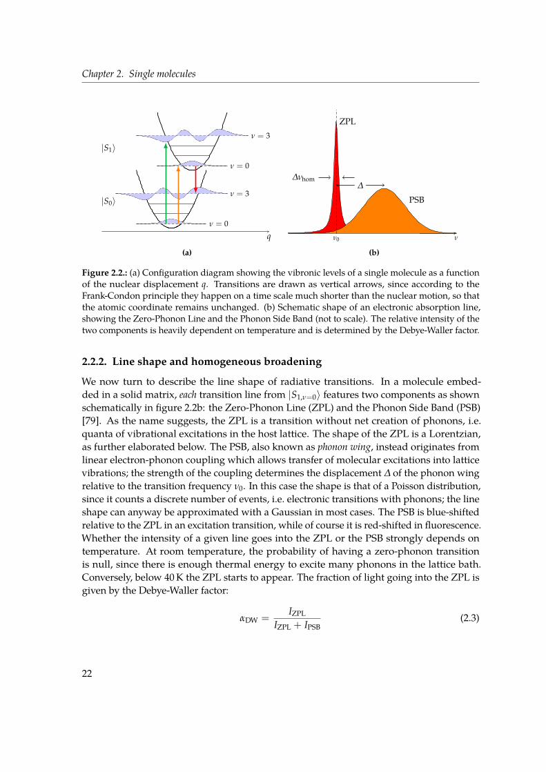
Chapter 2. Single molecules
ν = 0
ν = 3|S0〉
ν = 0
ν = 3
|S1〉
q
(a)
ν0 ν
ZPL
PSB∆
∆νhom
(b)
Figure 2.2.: (a) Configuration diagram showing the vibronic levels of a single molecule as a functionof the nuclear displacement q. Transitions are drawn as vertical arrows, since according to theFrank-Condon principle they happen on a time scale much shorter than the nuclear motion, so thatthe atomic coordinate remains unchanged. (b) Schematic shape of an electronic absorption line,showing the Zero-Phonon Line and the Phonon Side Band (not to scale). The relative intensity of thetwo components is heavily dependent on temperature and is determined by the Debye-Waller factor.
2.2.2. Line shape and homogeneous broadening
We now turn to describe the line shape of radiative transitions. In a molecule embed-ded in a solid matrix, each transition line from |S1,ν=0〉 features two components as shownschematically in figure 2.2b: the Zero-Phonon Line (ZPL) and the Phonon Side Band (PSB)[79]. As the name suggests, the ZPL is a transition without net creation of phonons, i.e.quanta of vibrational excitations in the host lattice. The shape of the ZPL is a Lorentzian,as further elaborated below. The PSB, also known as phonon wing, instead originates fromlinear electron-phonon coupling which allows transfer of molecular excitations into latticevibrations; the strength of the coupling determines the displacement ∆ of the phonon wingrelative to the transition frequency ν0. In this case the shape is that of a Poisson distribution,since it counts a discrete number of events, i.e. electronic transitions with phonons; the lineshape can anyway be approximated with a Gaussian in most cases. The PSB is blue-shiftedrelative to the ZPL in an excitation transition, while of course it is red-shifted in fluorescence.Whether the intensity of a given line goes into the ZPL or the PSB strongly depends ontemperature. At room temperature, the probability of having a zero-phonon transitionis null, since there is enough thermal energy to excite many phonons in the lattice bath.Conversely, below 40K the ZPL starts to appear. The fraction of light going into the ZPL isgiven by the Debye-Waller factor:
αDW =IZPL
IZPL + IPSB(2.3)
22

2.2. Optical properties of dye molecules in solid matrices
The Zero-Phonon Line of the purely electronic transition is called 00-ZPL, and it is the sourceof a fraction α equal to αFCαDW of the emitted fluorescence light. Rigid molecules tend tohave larger values of α, thus approaching the behaviour of a Two-Level System (TLS) (figure2.1b).Of all the Zero-Phonon Lines, the 00-ZPL is the most important one, since it is also the
narrowest one. Transitions ending in a vibrational level of the electronic ground state areindeed very broad, because of the short lifetime of the final state which is on the order ofpicoseconds. Conversely, the purely electronic line has a longer lifetime, in the 1–10 ns range.The lifetime τF of the |S1,ν=0〉 state is written in terms of the decay rates (reciprocals of τ) as
1τF
=1
τrad+
1τnrad
(2.4)
taking into account both radiative and non-radiative decays. All these processes determinea depopulation of the excited state and therefore contribute to the spectral broadening of thetransition line. Unfortunately, this is not the only source of broadening. In a solid environ-ment we also have to take into account dephasing of the wevefunction due to collisions withimpurities or lattice vibrations (phonons). These scattering processes destroy the coherenceof the wavefunction (yet without altering the population) therefore significantly increasingthe spectral width of the transition. This is often called pure dephasing to make a distinctionwith the damping of the wavefunction caused by population depletion. In the density matrixformalism, the off-diagonal elements, or coherences, are responsible for this kind of damping[80]. If we name T2 the total characteristic time of coherences, then the total dephasing rateis written as [1]:
Γ2 =1T2
=1
2T1+
1T∗2
(2.5)
where T1 = τF accounts for dephasing due to population decay, whereas T∗2 accounts fordephasing by population-conserving scattering processes2. The normalized line shapefunction of a ZPL is a Lorentzian3 [76, 79]:
I(ν− ν0) =1
4π2∆νhom
(ν− ν0)2 + (∆νhom/2)2 (2.6)
where the homogeneous linewidth γhom is related to the dephasing time of the opticaltransition by the following equation:
γhom = ∆νhom =1
πT2=
12πT1
+1
πT∗2(2.7)
2This notation dates back to Bloch’s original treatment of nuclear magnetic resonance [81]. A T2 process isalso called transverse relaxation because in the Bloch sphere representation it is given by a projection of theBloch vector on the z axis (thus conserving population); a T1 process is instead referred to as a longitudinalrelaxation since it does not conserve population [1].
3In a solid environment pseudolocal phonons can lead to deviations from a pure Lorentzian, resulting in amore complicated shape [82].
23

Chapter 2. Single molecules
While T1 is in practice independent of temperature, the pure dephasing time T∗2 instead dom-inates at room temperature but can be strongly suppressed by cryogenic cooling. The actualamount of pure dephasing depends on the excitation of low frequencymodes (local phonons,molecular librations4) that couple to the electronic transition of the dye molecule. In particu-lar, quadratic electron-phonon coupling results in a temperature dependent broadening ofthe ZPL by phonon scattering [79]. In a crystalline host matrix at cryogenic temperatures(T ≤ 4 K) T∗2 tends to infinity, therefore the ZPL is only limited by its natural broadeningwhich depends on the lifetime of the electronic excited state:
γnat = ∆νnat =1
2πT1(2.8)
In the simplest cases, we can express the linewidth as a function of temperature using theArrhenius law [83]:
γhom = γhom(0) + A exp(− Ea
kBT
)(2.9)
where Ea is the activation energy (equal to the energy of the local phonon or molecularlibration), γhom(0) = γnat and A depends on the strength of the electron-phonon coupling.When cooled down to cryogenic temperatures, a dye molecule in a solid matrix is thereforeable to deliver lifetime-limited photons through the fluorescence of the 00-ZPL.
2.2.3. Inhomogeneous broadening
To complete the picture about the spectral characteristics of molecules in solid matrices, weare left with discussing the effects that the host matrix itself has on the energy levels of theguest molecule. Indeed, the local environment surrounding a singlemolecule determines theexact energy of the electronic levels, and consequently the exact frequency of the excitationline. Local defects, random internal strain fields, crystal edges, impurities and dislocationsin the host matrix all contribute to create slightly different electrostatic environments fordifferent molecules. This results in the inhomogeneous broadening of the transition due toeach molecule feeling a different nanoenvironment in its immediate surroundings. Differentmolecules will therefore present transition frequencies centred on different values. Thedistribution of frequencies is a Gaussian, since the environmental fluctuations causingthis kind of broadening are different for each individual molecule. The inhomogeneousbroadening of the transition can be smaller than 1GHz in the best crystals, and as highas 10 THz (≈ 330 cm−1) in polymers [84, 85]. The amount of inhomogeneous broadeningis determined by the particular choice of the dye-matrix pair and even by the samplepreparation technique. For example, slowly grown crystals feature a linewidth distributionthat is typically smaller than for shock-frozen ones.
4Molecular librations are hindered rotations, or small oscillations around a preferential orientation.
24
2.3. Single-molecule detection: fluorescence excitation microscopy
As we will see, at cryogenic temperatures the inhomogeneous broadening of the lifetime-limited 00-ZPLs can be exploited to spectrally address individual molecules. The inhomo-geneous distribution of frequencies can also be viewed under a different light. Indeed, itshows how a molecule could be used as an extremely sensitive probe for the nanoscopicenvironment. Given that a lifetime-limited transition can be as narrow as a few MHz andconsidering that the optical transition frequency is of the order of 500 THz (visible light),the quality factor Q of the 00-ZPL can be as high as 108. It is therefore clear that very smallchanges in the nanoenvironment, such as weak perturbations produced by local electric,magnetic or strain fields, do cause a detectable shift in the resonance [86]. In absence ofother unwanted phenomena such as spectral diffusion, the line shift can therefore be usedas a sensitive probing tool for the local environment at the nanometre scale [87–90].
2.3. Single-molecule detection: fluorescence excitation microscopy
Optical detection of single molecules is conventionally accomplished by means of fluores-cence excitation spectroscopy: a light source (laser) excites the molecule and the resultingfluorescence is observed. The task of detecting a single molecule presents several experimen-tal challenges. Broadly speaking, two apparently simple conditions must hold. Firstly, atmost one molecule should be excited by the laser and, secondly, the resulting signal shouldbe efficiently collected and detected against background and dark counts from the detectors.In addition, the molecular system under investigation should be photostable over extendedperiod of times, have a quantum yield ideally close to unity and negligible bottleneck effects— originating from triplet or metastable states — which limit the fluorescence rate.
The first requirement, i.e. the optical isolation of a single molecule, can be ensured eitherspatially or spectrally, or by a combination of the two. In the first case, a very diluted samplewhere the molecule is embedded as an impurity within a transparent matrix is prepared, soas to ensure that a single molecule lies within the excitation spot. Tightly focused laser beamsthrough a microscope objective (spot diameter ≈ µm) also help in reducing the size of theprobed volume. At cryogenic temperatures, inhomogeneous broadening due to interactionswith the environment causes random shifts in the lifetime-limited lines. A narrow-bandlaser (linewidth ≈ 1 MHz) tuned into the wings of the inhomogeneous line, where fewermolecules are found, can therefore be used to successfully excite single molecules by spectralselection.
Excitation is usually done throughmicroscope objectives. They provide diffraction-limitedspot sizes and collect light over a wide solid angle, especially oil-immersion objectives. Infact, the same objective is often used both in excitation and collection, a configuration calledepifluorescence microscopy. In confocal excitation the sample is illuminated point by pointwith a diffraction-limited spot. Since only a small spot is illuminated, other parts of thesample are addressed by scanning either the spot itself or by moving the sample underneaththe excitation spot. Additionally, in single-molecule detection experiments this technique
25

Chapter 2. Single molecules
is often used in conjunction with a pinhole in the detection path, so as to prevent lightoriginating from out-of-focus planes on the sample to reach the detector, thus increasingcontrast and resolution. Conversely, in wide-field illumination a greater portion of the sampleis illuminated, as in a traditional microscope. Other experimental techniques include TotalInternal Reflection Fluorescence (TIRF) microscopy, in which a molecule is probed with theevanescent field generated upon total internal reflection at a boundary with a high refractiveindex contrast5, and Scanning Near-field Optical Microscopy (SNOM), in which excitation isdone through a small aperture such as a tapered, metal-coated fibre.
Collection and detection are other critical aspects of a single-molecule experiment. As an-ticipated, a high-Numerical Aperture (NA) objective is used to efficiently collect fluorescencefrom the sample. In general the excited dipole will not emit in the direction of the objective,therefore having a high NA also helps in ensuring that light emitted at high angles is stillcollected. Spectral filtering is needed to separate the red-shifted fluorescence signal from theexcitation light. Several optical elements, such as notch filters, longpass filters and dichroicmirrors can be used to this purpose. The elimination of background light is particularlycrucial. Background sources include residual laser emission in the spectral range of thedetected fluorescence, residual transmission of backscattered laser light through the filtersand fluorescence from the filters themselves. Additionally, impurities on the sample can alsogive rise to unwanted fluorescence, therefore special care has to be taken while preparingand handling the samples.
2.4. Overview of recent research
Dibenzoterrylene (DBT) molecules embedded in anthracene crystals (DBT:anth), the systemthat we are going to study in greater detail in the next chapter, have been proposed andsuccessfully operated as sensitive nanodetectors [91]. Recently, that system has been usedas a sort of nanomicrophone to probe acoustic strain, i.e. to detect localized low-frequencyacoustic vibrations, which is a first step towards detection and control of nanomechanicaloscillators by optical means [88, 90]. Detection of Stark shifts in single DBT molecules hasbeen used to investigate transport of electrical charge in organic crystals such as anthracenein a field-effect transistor configuration [92].
A lot of ongoing research closely related to single-molecule detection and sensing makesuse of optical antennas [93, 94] to optimize the energy transfer between a localized emitterand propagating light. Metallic nanoparticles have been used to enhance fluorescence ofweak emitters [95–97] and to enhance the rate of spontaneous emission [98, 99]. Furthermore,active research in the field of super-resolution microscopy using optical antennas is ongoing[100, 101]. Notable examples of important results enabled by the development of thesetechniques are the recent findings on single light-harvesting complexes [102], in whichquantum behaviours such as coherent energy transfer [103] and photon antibunching [104]
5This technique is typically employed for vertically oriented molecules to optimise polarization matching.
26

2.4. Overview of recent research
have been observed. Finally, optical antennas can also be used to direct single-moleculeemission and enhance collection efficiency [105–107].Organic dye molecules such as Dibenzanthanthrene (DBATT) and DBT have been suc-
cessfully used as single-photon sources [108, 109] and as such have been the subject ofseveral important experiments. Operation of single DBATTmolecules as an optical transistorhas been demonstrated [110]. Indistinguishable photons from remote DBATT moleculeshave been used to demonstrate two-photon interference [111] and to perform single-photonspectroscopy [112]. The latter is an important step towards the realization of nonlinearcoupling between few emitters and few propagating photons [113]. Coherent manipulationof single-molecule states is also actively investigated [114–116]. Very recently, new schemesfor efficient coherent interaction between light and single DBT molecules in a dielectricnanoguide have been proposed [117]. Indeed, from the point of view of applications, animportant achievement would be the implementation of large optical nonlinearities on achip, using single dye molecules as embedded single-photon sources [64].
In the following chapter we are going to present a particular combination of a matrix-dyesystem, based on single Dibenzoterrylene molecules embedded in thin anthracene crystals.We will perform a full optical characterisation of this system, highlighting its promisingcharacteristics as a single-photon source.
27


Chapter 3.
Spectroscopy and photophysics of single DBTmoleculesIn this chapter we present a specific system of emitters based on single Dibenzoterrylene moleculesembedded in a thin matrix of crystalline anthracene. The system looks very promising as a single-photon source and for sensing applications. Using a home-built epifluorescence scanning microscope,a full optical study is performed, aimed at characterizing several photophysical properties of theDBT:anth system. An overview of the employed methods is given, comprising sample fabrication andexperimental setup. Several properties are investigated at room temperature, such as fluorescencesaturation intensity, dipole orientation and emission pattern, fluorescence and triplet lifetime. Attemperatures down to 3K, we observe a lifetime-limited absorption line. Also, we demonstrate photonantibunching from this system. Finally, an AFM-based nanomanipulation technique is presented,allowing positioning of anthracene crystals at the sub-µm level.
3.1. DBT in anthracene crystals: an optimal dye-matrix match
Single molecule experiments typically involve samples in which the molecule under investi-gation is embedded as a dopant in a solid host matrix. Such a system ensures optical stabilityof the dye molecule and protects it against oxidation from quencher agents. A careful choiceof both the guest emitter and the host matrix must be made to obtain the best performance.Most works published so far have concentrated on the family of Polycyclic Aromatic Hy-drocarbons (PAH) as for the organic emitter. Typical investigated dye molecules includepentacene, terrylene, dibenzoterrylene (DBT) and dibenzantanthrene (DBATT, whereascommon host crystals are naphtalene and anthracene. Besides crystals, a host matrix canalso be a polymer — such as poly(styrene) (PS) and poly(metyl methacrylate) (PMMA) —or a so-called Shpol’skii matrix, such as frozen hexadecane, nonane and tetradecane. Ingeneral, molecular crystals are more attractive than other hosts, since they tend to embedthe guest molecule at well-defined insertion sites, resulting in particularly stable systemsand narrow Zero-Phonon Lines (ZPL) limited only by the excited state lifetime. On the otherhand, molecules embedded in polymer films are much more subject to spectral diffusionphenomena and photobleaching. A more comprehensive review of the most used dyes,hosts and their properties can be found in the literature [85, 86].The host-guest combination that we propose and study in this work is made of single
Dibenzoterrylene (DBT) molecules embedded in thin anthracene crystals (n ≈ 1.6). Asthe host matrix, anthracene has several advantages. It is cheap and can be easily purified
29
Chapter 3. Spectroscopy and photophysics of single DBT molecules
and handled; as detailed in section 3.2.1, thin anthracene crystals can be easily obtainedby means of spin coating or sublimation. Furthermore, anthracene is stable both at roomand cryogenic temperatures, without undergoing any phase transition during the cooldown process. Both DBT and anthracene are aromatic compounds, consisting of 8 and 3benzene rings respectively (figure 3.1b). Due to their similar chemical structure, DBT nicelyfinds its place within the crystalline structure of anthracene. Two main insertion sites havebeen identified [83]. Most molecules are embedded in the main insertion site with a 00-ZPLcentred at 785.1 nm at cryogenic temperatures; few molecules will instead end up in the redsite at 794.3 nm. The optical lines can be tuned by applying a Stark voltage [83, 88]. Theirproximity to the atomic lines of rubidium and potassium is of particular interest, indeedinterfacing of molecular photons to atomic alkali vapours has already been proposed as afundamental step towards the realization of quantum memories [118]. Furthermore, thespectral region covered by this system conveniently lies in the operating range of silicon-based photodetectors, whose detection efficiency peaks around 750 nm. Thanks to thegood structural match between host and guest, the Zero-Phonon Lines are very stableagainst photobleaching and spectral diffusion; indeed, the system has been shown to resistseveral hours of strong illumination [119]. The stability of the transition frequency is a verydesirable property, if the shift in the spectral line is to be used as a probe for electrical orother dynamical processes taking place at the nanoscale. In practice, the stability of theoverall system is only limited by the slow sublimation of the thin anthracene crystals atroom temperature, taking place over several days or weeks. A protective layer of poly(vinylalcohol) (PVA) can be deposited on top of the anthracene crystals to further increase thecrystals’ lifetime.
Other than for their similar chemical structure, the dye-matrix pair that we are studying isa good match also for the relative position of the energy levels. Indeed, in order to have highfluorescence count rates, the guest molecule should have a very weak Inter System Crossing(ISC) between the first excited singlet and triplet states (|S1〉 → |T1〉), so that the probabilitythat the molecule becomes momentarily trapped in the triplet state is low. When the host’striplet state lies at a lower energy than the guest’s singlet state, ISC in the guest molecule isstrongly facilitated, resulting in a weaker fluorescence signal that can make single moleculedetection impossible in the worst cases [120]. As a matter of fact, anthracene’s first tripletstate is located around 680 nm [121], that is to say at an energy well above DBT’s first excitedsinglet state (785 nm). The intersystem crossing yield is very low at 10−7 [83], and the tripletstate is short-lived, with a lifetime of 1.5µs [119]. The effect of the triplet state is thereforenegligible so that, in the absence of external loss channels, a DBT molecule in the excitedstate will relax through radiative decay with a Quantum Yield (QY) close to unity. All theproperties described so far make the DBT:anth system an ideal candidate for a stable andbright single-photon source.
Figure 3.1a shows the energy level structure of DBT in themain insertion site, as well as thetransitions involved in the different excitation and detection schemes. We usually performsingle-molecule experiments with individual DBT molecules by pumping the molecule, by
30

3.2. Methods
ν0ν1|S0〉ν2
ν0ν1|S1〉ν2
ν0ν1 |T1〉ν2
767n
m
00-ZPL
785n
m
fluorescence
ISC
(a)
760 780 800 820 840 860
wavelength (nm)
inte
nsity
(a.u
.)
(b)
Figure 3.1.: (a) Jablonski diagram for DBT molecules embedded in an anthracene crystal showingthe energy levels and the transitions used in the different excitation and detection schemes. (b)Fluorescence spectrum of DBT in anthracene, obtained with 767 nm excitation. The inset shows themolecular structure of DBT (top) and anthracene (bottom).
means of laser excitation, into a vibrational state of the first electronic excited state |S1〉 (modeat 300 cm−1, λexc = 767 nm). The molecule then quickly relaxes (in the ps time scale) to thefundamental vibrational mode of the first electronic excited state |S1,ν=0〉 through vibrationalrelaxation, a fast non-radiative process. The red-shifted fluorescence is then observed,originating from the decay to the vibrational modes of the |S0〉 state. This excitation schemeallows fluorescence from the 00-ZPL to be collected, but is not suitable for spectral selectionof single molecules at cryogenic temperatures, as the excitation linewidth is of the order of40GHz at 2K [109]. Instead, excitation spectra at cryogenic temperatures are investigatedby pumping the 00-ZPL at 785 nm (resonant excitation). Below 4K indeed, dephasing due tophonons vanishes and the line becomes almost lifetime-limited, showing a natural width ofabout 40MHz corresponding to a lifetime of 4.2 ns. Because of inhomogeneous broadening,different molecules will have this transition centred at different energies, as their levels areshifted depending on the environment inside the crystalline matrix; thanks to its narrowwidth, the 00-ZPL transition can therefore be used to spectrally address single moleculesbelow 4K (figure 3.3b).
3.2. Methods
3.2.1. Sample preparation
One advantage of our systemof emitters is that anthracene crystals embeddingDBTmoleculesare relatively easy to fabricate. Depending on the application and type of measurement,we consider two different fabrication techniques that yield different kinds of crystals: spin-coating and co-sublimation [119, 122].
31
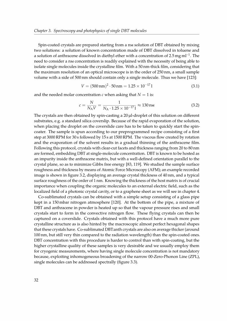
Chapter 3. Spectroscopy and photophysics of single DBT molecules
Spin-coated crystals are prepared starting from a nm solution of DBT obtained by mixingtwo solutions: a solution of known concentration made of DBT dissolved in toluene anda solution of anthracene dissolved in diethyl ether with a concentration of 2.5mgml−1. Theneed to consider a nm concentration is readily explained with the necessity of being able toisolate single molecules inside the crystalline film. With a 50 nm-thick film, considering thatthe maximum resolution of an optical microscope is in the order of 250 nm, a small samplevolume with a side of 500 nm should contain only a single molecule. Thus we have [123]:
V = (500 nm)2 · 50 nm = 1.25× 10⁻¹⁷ l (3.1)
and the needed molar concentration c when asking that N = 1 is:
c =N
NAV=
1NA · 1.25× 10−17 l
≈ 130 nm (3.2)
The crystals are then obtained by spin-casting a 20µl-droplet of this solution on differentsubstrates, e.g. a standard silica coverslip. Because of the rapid evaporation of the solution,when placing the droplet on the coverslide care has to be taken to quickly start the spin-coater. The sample is spun according to our preprogrammed recipe consisting of a firststep at 3000RPM for 30 s followed by 15 s at 1500RPM. The viscous flow created by rotationand the evaporation of the solvent results in a gradual thinning of the anthracene film.Following this protocol, crystals with clear-cut facets and thickness ranging from 20 to 80 nmare formed, embedding DBT at single-molecule concentration. DBT is known to be hosted asan impurity inside the anthracene matrix, but with a well-defined orientation parallel to thecrystal plane, so as to minimize Gibbs free energy [83, 119]. We studied the sample surfaceroughness and thickness by means of Atomic Force Microscopy (AFM); an example recordedimage is shown in figure 3.2, displaying an average crystal thickness of 40 nm, and a typicalsurface roughness of the order of 1 nm. Knowing the thickness of the host matrix is of crucialimportance when coupling the organic molecules to an external electric field, such as thelocalized field of a photonic crystal cavity, or to a graphene sheet as we will see in chapter 4.Co-sublimated crystals can be obtained with a simple setup consisting of a glass pipe
kept in a 150mbar nitrogen atmosphere [120]. At the bottom of the pipe, a mixture ofDBT and anthracene in powder is heated up so that the vapour pressure rises and smallcrystals start to form in the convective nitrogen flow. These flying crystals can then becaptured on a coverslide. Crystals obtained with this protocol have a much more purecrystalline structure as is also hinted by the macroscopic almost perfect hexagonal shapesthat these crystals have. Co-sublimatedDBT:anth crystals are also on average thicker (around100 nm, but still very thin compared to the radiation wavelength) than the spin-coated ones.DBT concentration with this procedure is harder to control than with spin-coating, but thehigher crystalline quality of these samples is very desirable and we usually employ themfor cryogenic measurements, where having single molecule concentration is not mandatorybecause, exploiting inhomogeneous broadening of the narrow 00-Zero-Phonon Line (ZPL),single molecules can be addressed spectrally (figure 3.3).
32

3.2. Methods
0 10 20 300
10
20
30
µm
µm
0
20
40
60
80
100
nm(a)
0 5 1030
40
50
60
70
µm
nm
(b)
Figure 3.2.: (a) Typical AFM topography image of a spin-coated anthracene crystal. Following ourfabrication protocol, crystals with clear-cut facets and thickness ranging from 20 to 80 nm are formed.(b) Cross section showing the crystal thickness profile along the red line in panel (a).
(a) (b)
Figure 3.3.: (a) SEM image of a co-sublimated anthracene crystal with its typical hexagonal shape.(b) Fluorescence image in wide field illumination from DBT molecules embedded in a co-sublimatedanthracene crystal at a temperature of 3K. The hexagonal shape of the crystal is clearly visible thanksto a guiding effect of light along the crystal perimeter (nanthracene ≈ 1.6). This image is obtainedfrom the superposition of 350 frames taken while varying the laser excitation frequency in a 3GHzrange. As the laser frequency is scanned, different single molecules are turned on/off thanks to theinhomogeneous broadening of the narrow 00-ZPL. Animated version available online [124].
33

Chapter 3. Spectroscopy and photophysics of single DBT molecules
3.2.2. Experimental setup
To perform single molecule spectroscopy and study the photophysics of our DBT:anthsystem,weuse a home-built, versatile epifluorescence scanningmicroscope. In epifluorescenceconfiguration, the same objective is used both to excite the sample and to collect fluorescence.Figure 3.4 shows a simplified version of the setup, whichwe are here going to briefly describe.
Excitation arm
At the head of the excitation arm, we use several laser sources depending on the moleculartransition that we want to excite and the type of measurement that we want to perform. Weemploy two narrowband (linewidth ≈ 1 MHz) Toptica tunable single-mode diode lasers: aDL100 External Cavity Diode Laser (ECDL) emitting at 785 nm and a DL DFB (DistributedFeedBack), emitting at 767 nm. These are Continuous-Wave (CW) lasers, while for lifetimemeasurementswe employ a pulsed Ti:sapphire laser (Tsunami by Spectra-Physics) optimizedto emit 200 fs-long pulses at 767 nm. A white light (WL) lamp is instead used for simpleimaging of the sample.As far as the diode lasers are concerned, optical isolators prevent scattered light to be
reflected back into the laser head; additional elements such as anamorphic prism pairsand cylindrical lenses (not shown) are used to optimize the laser spot into a collimatedcircular shape. The laser beams are monitored for stability with a Fabry-Pérot cavity and anoscilloscope. Laser light is then coupled to a polarization-maintaining single-mode opticalfibre with a core diameter of 4µm. At the entrance of the fibre, we place a polarizing beamsplitter cube and two half-wave plates. The first plate is used to adjust the power transmittedby the beam splitter, while the second one is used to rotate the linear polarization to matchthat of the fibre. At the fibre output, a bandpass (BP) filter (Semrock FF01-769/41, TBP01-790/12) is used to remove unwanted spectral components and residual fluorescence fromthe laser beam.Following the light path along the excitation arm, a half-wave plate is used to rotate
the polarization while neutral density filters are used to attenuate the beam as needed.A widefield (WF) lens can be used for fluorescence imaging. Indeed, when this lens isinserted, the laser beam is focused onto the objective back-aperture, causing a wider area(≈ 20 × 20 µm) to be illuminated on the sample than in confocal excitation. Finally, adichroic mirror (Semrock FF776-Di01) sends the excitation light to the sample while lettingthe collected fluorescence light into the detection box.
Sample accommodation
The final segment of the excitation path is divided into two independent lines, one for roomtemperature measurements and another one for cryogenic cooling. The cryostat that weuse for low temperature measurements is the Cryostation by Montana Instruments. It is aclosed cycle helium cryostat, specifically designed for fluoresce confocal microscopy. The
34

3.2. Methods
cryost
at
EMCCDEM
CC
D
EC
DL
Ti:sa
OI
DM GM
λ/2
λ/2
fiber
NA
=1.4
NA
=0.7
WL
WF
λ/2
PH
APD
APD
piezoBP
LP
ND
Figure 3.4.: Simplified diagram of the experimental setup. CW laser diodes emitting at 767 nm and785 nm are used to excite the 0-1 and 0-0 transitions, respectively. A pulsed Ti:sa laser emitting200 fs-long pulses at 767 nm is used for lifetime measurements. A white light lamp (WL) is used toimage the sample, whereas a widefield lens (WF) can be inserted to perform fluorescence imaging.High Numerical Aperture (NA) objectives are used to efficiently collect fluorescence light. Samplescan be mounted either on a piezo stage for room temperature measurements or inside a cryostat formeasurements down to 3K. In the latter case, the laser spot is scanned on the sample by using agalvo mirror (GM) and a telecentric system. Detection devices are placed inside a box which acts asa shield for residual light. They comprise two Avalanche Photo Diodes (APDs) arranged in HanburyBrown – Twiss configuration, an EM-gain CCD camera and a grating spectrograph. A telescope anda pinhole (PH) act as a spatial filter, increasing resolution and contrast.
35

Chapter 3. Spectroscopy and photophysics of single DBT molecules
sample is mounted inside the cryostat’s vacuum chamber, at the top of a cold finger. A lowworking distancewindowensures optical access and allows regular room temperature opticalcomponents to be placed as close as 1mm from the cooled sample. In this configurationwe use an air objective with NA = 0.7 and a working distance of 6mm (Mitutoyo 100XPlan Apochromat). The excitation light enters the objective through a telecentric system.Together with a dual-axis galvo mirror, the telecentric system allows the laser spot to bescanned over different points on the sample. This is necessary since at the moment we don’thave a system of nanopositioners inside the cryostat chamber.
For room temperature measurement, the sample is mounted on a piezoelectric nanoposi-tioner (NanoCube® by Physik Instrumente), which in turn is fixed on a dual-axis goniometerand amanual translation stage for coarse positioning. In this case an air objective can be used,but most often we use an oil-immersion objective for a much greater Numerical Aperture(Zeiss Plan Apochromat, 100X, NA=1.4).
Detection box
All detection devices are placed inside a box to shield them from non-signal light. Fluores-cence light collected through the objective enters the detection box through the dichroicmirror and a longpass (LP) filter (Semrock RazorRedge®-785RS-25) to selectively let into thebox only the red-shifted fluorescence and cut residual excitation light. A telescope systemand a pinhole act as a spatial filter, by cutting light originating from out-of-focus planeson the sample and from nearby emitters, thus greatly increasing resolution and contrast.Two APDs arranged in Hanbury Brown – Twiss (HBT) configuration are used for Time-Correlated Single Photon Counting (TCSPC) measurements in conjunction with PicoHarp,a standalone TCSPC system by PicoQuant. The APDs that we use are τ-SPAD-50 SinglePhoton CountingModules by PicoQuant; they feature low dark count rates (< 50 cps), shortdead time (< 70 ns) and detection efficiency up to 70%. Alternatively, light can be focusedon an EM gain (Electron-Multiplying) CCD camera (Andor iXon 885, 1004× 1002 pixels,pixel size 8 µm× 8 µm) for fluorescence or white-light imaging. When enabled, EM gainensures high performance in low light scenarios, thanks to the generation of secondaryelectrons via impact-ionization processes. Finally, light can be spectrally analysed using agrating spectrograph (Andor Shamrock 303i).
3.2.3. Data acquisition and control software
The experimental setup described in the previous subsection comprises several electronicdevices that must be operated together and with the proper timings in order for the experi-ment to be run smoothly. A dedicated acquisition software, tailored to our specific needs,not only guarantees the optimal functioning of the overall setup but also allows to automatecrucial phases of the data taking procedures. To meet these requirements and to ease theexperimental workflow during everyday operations, a complete measurement and control
36

3.2. Methods
software was developed from scratch entirely in the framework of this present thesis. Abrief description of its functionalities and structure is therefore given in this section. Oursoftware is also featured on National Instruments’ catalogue of case studies [125].The control software was initially prototyped in its early form using LabVIEW, the
widespread platform from National Instruments for data acquisition, instrument con-trol and automation. With time and a growing need to add more features to the software,continuing development with LabVIEW became impractical so that a new version of the soft-ware was entirely rewritten following a new approach. The new software is written in C++,a widely used high-level programming language, and makes use of the Qt libraries whichprovide the main application framework and user interface (UI). Since C++ is an object-oriented programming language, the source code is highly modularized and abstracted intoreusable components that make development easier and will allow easy integration of newhardware in the future. As new features were added, the source base grew considerablyin size, reaching 9286 Single Lines Of Code (SLOC) at the time of writing. The UI is conve-niently organized in detachable tabs, each dedicated to a single instrument or a specificmeasurement (figure 3.5).
Themain purpose of the software is to control the PCIe6351 Data Acquisition (DAQ) boardfrom National Instruments. To do so, it makes use of the vendor-provided NI-DAQmxprogramming libraries for C/C++. Of all the features onboard the multifunction card,the control software makes heavy use of the digital counters in order to count the singlephotons seen by the APDs; indeed the τ-SPAD generates a digital TTL pulse upon detectinga single photon. An additional digital counter, internal to the board, is configured as a gatingcounter to enable/disable counting during an integration cycle, so that the exposure timingis performed in hardware rather than in software. The measured count rates are displayedin real time which is useful to perform alignment operations on the optical table.
Acquisition of count rates is most useful when done in sync with some action performedby an actuator on the experimental setup. For example, we use an analogue output channelof the DAQ card to drive the grating movement inside the tunable diode laser, which resultsin a detuning of the laser frequency. The software makes it possible to measure fluorescencecount rates while varying the excitation laser frequency; this allows for example to measurethe width of a molecular absorption line as presented in section 3.3.4. A remarkable opportu-nity for measurement automation comes from the possibility to acquire fluorescence countrates while physically scanning the sample under the objective, so that the laser confocal spotilluminates different points on the sample. The software allows to collect a fluorescence map ofa portion of a sample, by sending through the serial port the appropriate commands to movethe piezo NanoCube® horizontally in the sample plane. For each pixel of the fluorescencemap, photon counts are measured while the piezo stage dwells in position for the specifiedintegration time, then the software moves the sample to the adjacent pixel repeating thecount rate measurement. With this procedure, fluorescence maps such as the one shown infigure 3.6a are acquired. When the sample is mounted inside the cryostation, scanning is
37

Chapter 3. Spectroscopy and photophysics of single DBT molecules
(a)
(b)
Figure 3.5.: Screenshots of the custom data acquisition and control software. (a) Interface to PicoHarpfor TCSPC measurements showing an antibunching measurement with live fitting. (b) Interface forfluorescence scan using the piezo translational stage or the galvo mirrors. An acquired fluorescencemap is shown, with single molecules automatically tagged.
38

3.3. Optical characterization
instead performed bymoving the galvo head placed at the pivot point of a telecentric system,so that the laser confocal spot is directed to different points on the sample. The softwareoversees the movement of the two galvo mirrors separately, by sending an analogue voltagethrough two analogue output channels of the DAQ board. The acquisition of a fluorescencemap is often the very first step of a measurement session, since it allows single moleculesto be easily identified as diffraction-limited spots. Indeed, for the sake of convenience thesoftware allows single points to be labelled on the map: single molecules can be taggedautomatically — by looking for spots with a signal to noise ratio above a certain threshold— or specified manually on the map. Once a fluorescence scan has been acquired and themolecules have been tagged, it is possible to move the excitation spot directly on a givenmolecule to perform other measurements. Manual controls are also available, allowing afine control of both sample position and laser focus.In addition to controlling the piezo translational stage and the DAQ board, the software
also interfaces directly with the PicoHarpmodule via the proprietary programming librariesprovided by PicoQuant. It is therefore possible to collect time-resolved measurementsdirectly from within our custom software, while having access to the full range of theinstrument’s configuration options. Additionally, antibunching and lifetime curves maybe fitted in real time during the data-taking process. Speaking again of automation, time-resolved measurements can be taken automatically by sequentially moving the sample onmolecules that have been previously marked on the fluorescence map. This feature is veryconvenient in that it could be used for example to considerably shorten the time needed tocollect lifetime measurements on many molecules, not only making it possible to collecthigher statistics in less time, but also making the measurements themselves less sensitiveto instabilities or drifts in the setup. In the future, by fully exploiting the combination oftime-resolved measurements and sample scanning, the software can be easily expanded totake lifetime maps, for example to image a graphene flake by taking lifetime measurementsof a layer of dyes deposited on top of it (figure 4.5).
Finally, our custom software also allows to control flippable mounts on the optical table —such as the mirror in front of the CCD camera and the pinhole acting as a spatial filter — bysending a toggle pulse either through an analogue or a digital output channel of the DAQcard.
3.3. Optical characterization
In this section we present a complete optical characterization of singleDBTmolecules embed-ded in a thin anthracene crystal. The measurements here discussed allow us to test the newlybuilt experimental setup and assess its performance, as well as build a knowledge of thetypical expected values for the experimental observables. When appropriate, we will alsohighlight how the observed optical properties relate to the characteristics of single-photonsources as described in section 1.3. Unless otherwise specified, all measurements were taken
39

Chapter 3. Spectroscopy and photophysics of single DBT molecules
0 2 4 6 8 100
2
4
6
8
10
µm
µm
20
40
60
80
kcou
nt/s
(a)
0 20 40 60
0.5
1
τ (ns)
norm
.coi
ncid
ence
s
(b)
Figure 3.6.: (a) Typical confocal fluorescence scan showing single DBTmolecules as diffraction-limitedspots. (b) Measured coincidences from a single DBT molecule (total integration time 900 s, laserpower 150µW). The strong reduction (93%) of the detected coincidences at zero time delay is a clearindication of the quantum nature of the observed light.
at room temperature on single DBTmolecules in spincoated anthracene crystals, exciting the0-1 transition with a CW laser at 767 nm. Excitation spectra at cryogenic temperatures wereinstead investigated on sublimated crystals, exciting the resonant 0-0 transition at 785 nm.Finally, fluorescence lifetime measurements were taken using a pulsed Titanium-Sapphire(Ti:sa) laser at 767 nm.
3.3.1. Photon antibunching
While time-resolved measurements will be presented as the last two sub-topics of thissection, we nonetheless start this overview by studying the photon statistics of the collectedfluorescence light. Indeed, ideally the first step to undertake before studying whicheveroptical property is to make sure that the observed fluorescence originates from a single DBTmolecule. As explained previously, at room temperature single molecule selection can onlybe achieved by ensuring that exactly one molecule is found underneath the laser excitationspot. In practical terms, this is tantamount to a sample prepared with a very low DBTconcentration. The ultimate proof that the diffraction-limited spots observed in a confocalscan as the one shown in figure 3.6a really do originate from a single molecule is to look forphoton antibunching in a coincidence correlation measurement.
Coincidences between photon counting events are acquired with the PicoHarp, to whichthe two APDs arranged in Hanbury Brown – Twiss (HBT) configuration are connected.Figure 3.6b shows the histogram of the observed coincidences from a single DBT moleculein CW excitation, featuring a strong antibunching dip. The experimental data is fitted at
40

3.3. Optical characterization
short delays with the function
g(2)(τ) = 1− b exp(−|τ|
∆t
)(3.3)
where ∆t accounts for the excitation and spontaneous emission rates [109, 126] and b, thedip depth, is found to be 93% in the measurement shown. Such a strong reduction of thedetected coincidences at zero time delay is a clear indication of the quantum nature of theobserved light, since a new excitation-emission cycle is necessary for a single quantumsource to emit a second photon, which requires an average delay. If the emitter is excitedwith an intense and short trigger pulse, exactly one photon will be emitted after an averagetime equal to the radiative lifetime, i.e. we can use our DBT:anth system as a source ofon-demand single photons [109].Photon statistics is critically affected by optical losses and noise, therefore a high SNR
is required to observe a pronounced antibunching dip. Indeed, background photons areresponsible for false start-stop measurements, leading to coincidence counts higher than 0at zero delay. The depth of the observed dip can be understood in terms of the expectedprobabilities to detect fluorescence signal (S) or background counts (BG):
PS =IS
IS + IBGPBG =
IBGIS + IBG
(3.4)
The expected value for the correlation function at zero delay is thus:
g(2)(0) = PSPBG + PBGPS + PSPS + PBGPBG ≈ 2PSPBG + PBGPBG (3.5)
where we have neglected the probability to detect two fluorescence photons simultaneously(antibunching). For the reported measurement, we have a typical count rate of 300 kcpsfor the fluorescence signal and 15 kcps for the background noise (SNR≈ 20), yielding anexpected reduction of the observed coincidences of 1− g(2)(0) ≈ 91 %.
3.3.2. Saturation behaviour
Having a high signal to noise ratio is a crucial requirement to perform Single MoleculeSpectroscopy (SMS) successfully. In order to maximize the fluorescence emission rate,the molecule must be pumped to the excited state with high probability. It is thereforeimportant to understand the saturation behaviour of the emitter in order to choose theproper excitation power. For example, when the highest count rates are desired, it is bestnot to exceed saturation intensity, as doing so would have the sole effect of increasing thebackground due to residual unfiltered laser light and matrix fluorescence, in addition toincreasing the likelihood of photobleaching.If we call σp the absorption cross section and Ii the excitation intensity, to a first approx-
imation the rate of absorption Γa is given by σp Ii [127], or equivalently the probability of
41
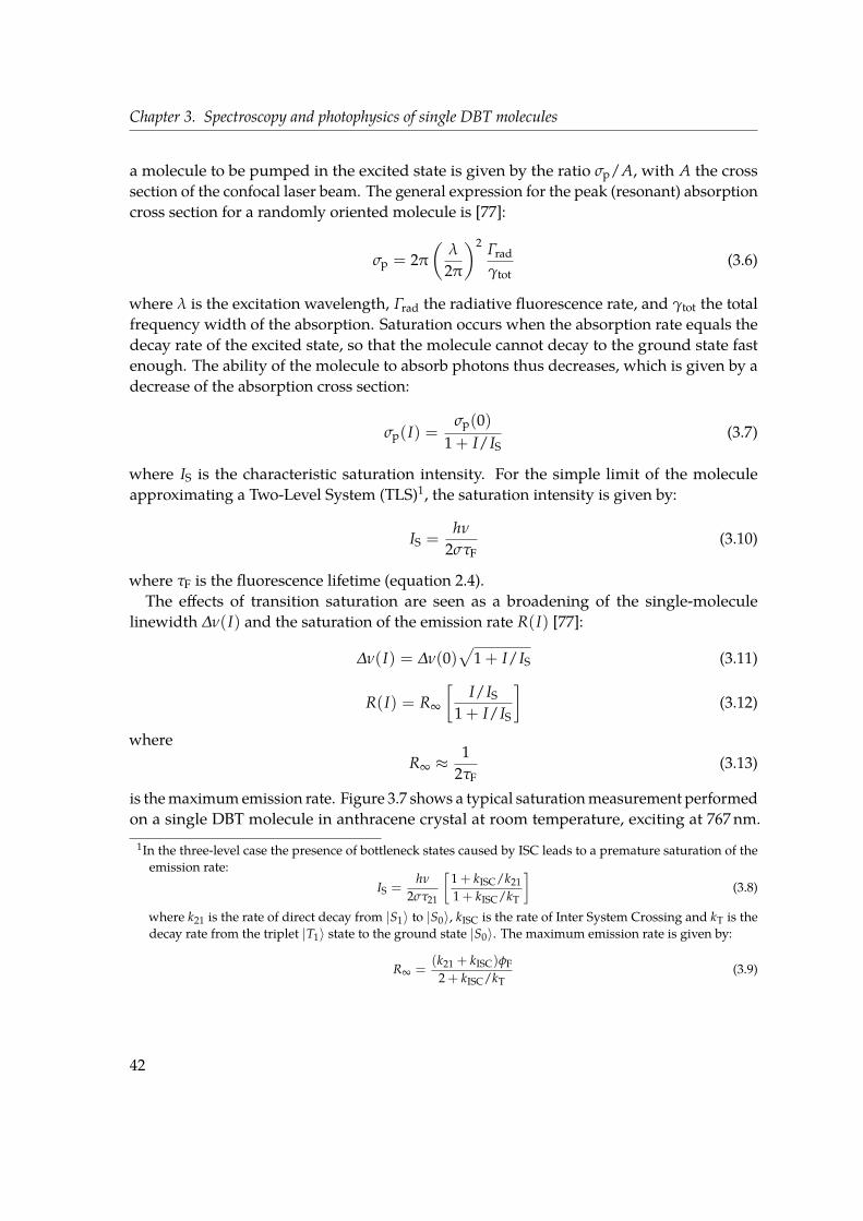
Chapter 3. Spectroscopy and photophysics of single DBT molecules
a molecule to be pumped in the excited state is given by the ratio σp/A, with A the crosssection of the confocal laser beam. The general expression for the peak (resonant) absorptioncross section for a randomly oriented molecule is [77]:
σp = 2π(
λ
2π
)2 Γradγtot
(3.6)
where λ is the excitation wavelength, Γrad the radiative fluorescence rate, and γtot the totalfrequency width of the absorption. Saturation occurs when the absorption rate equals thedecay rate of the excited state, so that the molecule cannot decay to the ground state fastenough. The ability of the molecule to absorb photons thus decreases, which is given by adecrease of the absorption cross section:
σp(I) =σp(0)
1 + I/IS(3.7)
where IS is the characteristic saturation intensity. For the simple limit of the moleculeapproximating a Two-Level System (TLS)1, the saturation intensity is given by:
IS =hν
2στF(3.10)
where τF is the fluorescence lifetime (equation 2.4).The effects of transition saturation are seen as a broadening of the single-molecule
linewidth ∆ν(I) and the saturation of the emission rate R(I) [77]:
∆ν(I) = ∆ν(0)√
1 + I/IS (3.11)
R(I) = R∞
[I/IS
1 + I/IS
](3.12)
whereR∞ ≈
12τF
(3.13)
is themaximumemission rate. Figure 3.7 shows a typical saturationmeasurement performedon a single DBT molecule in anthracene crystal at room temperature, exciting at 767 nm.1In the three-level case the presence of bottleneck states caused by ISC leads to a premature saturation of theemission rate:
IS =hν
2στ21
[1 + kISC/k211 + kISC/kT
](3.8)
where k21 is the rate of direct decay from |S1〉 to |S0〉, kISC is the rate of Inter System Crossing and kT is thedecay rate from the triplet |T1〉 state to the ground state |S0〉. The maximum emission rate is given by:
R∞ =(k21 + kISC)φF
2 + kISC/kT(3.9)
42
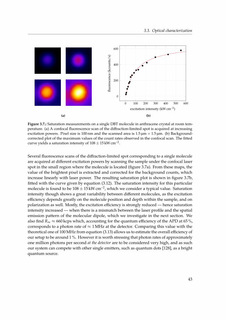
3.3. Optical characterization
(a)
0 100 200 300 400 500 600
0
200
400
600
excitation intensity (kWcm−2)flu
orescenc
e(kcoun
ts/s
)
(b)
Figure 3.7.: Saturation measurements on a single DBT molecule in anthracene crystal at room tem-perature. (a) A confocal fluorescence scan of the diffraction-limited spot is acquired at increasingexcitation powers. Pixel size is 100 nm and the scanned area is 1.5 µm× 1.5 µm. (b) Background-corrected plot of the maximum values of the count rates observed in the confocal scan. The fittedcurve yields a saturation intensity of 108± 15 kWcm−2.
Several fluorescence scans of the diffraction-limited spot corresponding to a single moleculeare acquired at different excitation powers by scanning the sample under the confocal laserspot in the small region where the molecule is located (figure 3.7a). From these maps, thevalue of the brightest pixel is extracted and corrected for the background counts, whichincrease linearly with laser power. The resulting saturation plot is shown in figure 3.7b,fitted with the curve given by equation (3.12). The saturation intensity for this particularmolecule is found to be 108± 15 kWcm−2, which we consider a typical value. Saturationintensity though shows a great variability between different molecules, as the excitationefficiency depends greatly on the molecule position and depth within the sample, and onpolarization as well. Mostly, the excitation efficiency is strongly reduced — hence saturationintensity increased — when there is a mismatch between the laser profile and the spatialemission pattern of the molecular dipole, which we investigate in the next section. Wealso find R∞ ≈ 660 kcps which, accounting for the quantum efficiency of the APD at 65%,corresponds to a photon rate of ≈ 1 MHz at the detector. Comparing this value with thetheoretical one of 100MHz from equation (3.13) allows us to estimate the overall efficiency ofour setup to be around 1%. However it is worth stressing that photon rates of approximatelyone million photons per second at the detector are to be considered very high, and as suchour system can compete with other single emitters, such as quantum dots [128], as a brightquantum source.
43
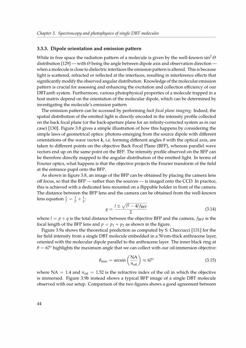
Chapter 3. Spectroscopy and photophysics of single DBT molecules
3.3.3. Dipole orientation and emission pattern
While in free space the radiation pattern of a molecule is given by the well-known sin2 Θ
distribution [129] —with Θ being the angle between dipole axis and observation direction—when amolecule is close to dielectric interfaces the emission pattern is altered. This is becauselight is scattered, refracted or reflected at the interfaces, resulting in interference effects thatsignificantlymodify the observed angular distribution. Knowledge of themolecular emissionpattern is crucial for assessing and enhancing the excitation and collection efficiency of ourDBT:anth system. Furthermore, various photophysical properties of a molecule trapped in ahost matrix depend on the orientation of the molecular dipole, which can be determined byinvestigating the molecule’s emission pattern
The emission pattern can be accessed by performing back focal plane imaging. Indeed, thespatial distribution of the emitted light is directly encoded in the intensity profile collectedon the back focal plane (or the back-aperture plane for an infinity-corrected system as in ourcase) [130]. Figure 3.8 gives a simple illustration of how this happens by considering thesimple laws of geometrical optics: photons emerging from the source dipole with differentorientations of the wave vector k, i.e. forming different angles θ with the optical axis, aretaken to different points on the objective Back Focal Plane (BFP), whereas parallel wavevectors end up on the same point on the BFP. The intensity profile observed on the BFP canbe therefore directly mapped to the angular distribution of the emitted light. In terms ofFourier optics, what happens is that the objective projects the Fourier transform of the fieldat the entrance pupil onto the BFP.As shown in figure 3.8, an image of the BFP can be obtained by placing the camera lens
off focus, so that the BFP — rather than the sources — is imaged onto the CCD. In practice,this is achieved with a dedicated lens mounted on a flippable holder in front of the camera.The distance between the BFP lens and the camera can be obtained from the well-knownlens equation 1
f = 1p +
1q :
q =l ±√
l2 − 4l fBFP2
(3.14)
where l = p + q is the total distance between the objective BFP and the camera, fBFP is thefocal length of the BFP lens and p = p1 + p2 as shown in the figure.Figure 3.9a shows the theoretical prediction as computed by S. Checcucci [131] for the
far field intensity from a single DBT molecule embedded in a 50 nm-thick anthracene layer,oriented with the molecular dipole parallel to the anthracene layer. The inner black ring atθ = 67° highlights the maximum angle that we can collect with our oil-immersion objective:
θmax = arcsin(NAnoil
)≈ 67° (3.15)
where NA = 1.4 and noil = 1.52 is the refractive index of the oil in which the objectiveis immersed. Figure 3.9b instead shows a typical BFP image of a single DBT moleculeobserved with our setup. Comparison of the two figures shows a good agreement between
44

3.3. Optical characterization
objective BFP lensobj. BFP CCDsources
A
B
fBFP
p2p1
q
pinhole
telescopefoc. pl. foc. pl.
φθ
Figure 3.8.: Schematic representation of the optical configuration used to acquire Back Focal Plane(BFP) images. Light emerging from the source dipoles with different orientations of the wave vectork is taken to different points on the objective BFP, which is imaged onto the CCD with the BFP lens.A spatial filter made of a telescope and a pinhole cuts light from nearby unwanted molecules on thesource plane and on out-of-focus planes, increasing resolution and contrast.
θ
0
0.2
0.4
0.6
0.8
1
0
45
90
135
180
225
270
315
φ
(a)
p-pol
s-po
l
(b)
−60−40−20 0 20 40 60
θ (deg)
norm
.int
ensi
ty
s-polp-pol
(c)
Figure 3.9.: (a) Theoretical prediction for the normalized intensity, collected on a plane in the far field,from a dipole embedded in a 50 nm-thick anthracene layer emitting at 785 nm (in-plane orientation,see S. Checcucci [131] for more details). The black circle at θ = 67° shows themaximum angle that ourobjective can collect (NA = 1.4). φ is the azimuthal angle on the BFP. (b) BFP image of a single DBTmolecule in confocal illumination (excitation power: 25µW; integration time: 2 s) after backgroundsubtraction and despeckling, observedwith our setup. (c) Cross cuts showing the angular distributionof the emitted light along the s and p polarizations. Dashed lines are theoretical predictions [131].
45

Chapter 3. Spectroscopy and photophysics of single DBT molecules
90
60
300
30
60
90
120
150180
150
120
0 0.5 1
(a)
90
60
300
30
60
90
120
150180
150
120
0 5 10 15
s polp pol
(b)
Figure 3.10.: (a) Normalized emission pattern in polar coordinates showing the total power densityas a function of the emission angle θ, as predicted from the theoretical model [131]. The emissionpattern is strongly modified compared to the free space case, exhibiting two side lobes . (b) Crosscuts showing the power density for the two s and p polarizations.
the theoretical model and the observed profile. The radial distance h of a point on the BFPimage can be related to the emission angle θ by noting that h(θ) = fobjnoil sin θ. Figure3.9c shows crosscuts of the BFP image along the two cross sections corresponding to sand p polarizations. The dipole emission pattern is strongly modified compared to thefree space case, featuring two side lobes — that are best appreciated in figure 3.10 — atangles greater than the critical angle θc = arcsin (nair/nanth) ≈ 39°, where nanth ≈ 1.6 isanthracene’s refractive index. Supercritical emission is a typical phenomenon of dipolesclose to interfaces in the near field, and is the result of the conversion of evanescent wavesinto travelling waves [132].
Different single molecules exhibit very similar emission patterns, the geometry of whichallows us to conclude that DBT molecules are embedded inside anthracene with their dipolepreferentially parallel to the crystal plane [130, 133], or at most out of plane by just a fewdegrees, in agreement with previous studies [83, 119]. Since the dipole emission pattern isstrongly influenced by its surrounding environment, engineering of the angular distributionof the emission of a single molecule can be achieved by embedding DBT molecules ina multilayer structure made not only of anthracene but also other dielectric, metallic orpolymeric layers [131]. Being able to tailor the spatial distribution of light coming from asingle molecule is indeed crucial — for example when coupling with some other photonicnanostructure is desired, or to channel light within the objective acceptance angles in such away to increase collection efficiency — and is therefore advised as a promising direction forfuture research.
46

3.3. Optical characterization
0 2 4 6 8 100
200
400
600
800
1 000
temperature (K)
∆ν h
om(M
Hz)
(a)
−400 −200 0 200 400
3 000
4 000
5 000
6 000
detuning (MHz)
coun
ts(b)
Figure 3.11.: (a) Linewidth dependence on temperature for DBTmolecules in anthracene crystal (mainsite) showing the exponential increase given by the Arrhenius law, modelled after the measurementsby Nicolet et al. [83]. (b) Resonant excitation spectrum of a single DBT molecule measured at atemperature below 3K. Fitting a Lorentzian yields a natural linewidth of 42± 1MHz.
3.3.4. Resonant excitation linewidth at cryogenic temperatures
As we have outlined in section 1.3, many applications of single-photon sources requirephotons that must be completely indistinguishable. In an ideal two-level system, purespontaneous emission generates photons that are truly indistinguishable and with thenatural linewidth determined only by the excited state lifetime. In reality (section 2.2.2), ina solid environment pure optical dephasing originating from scattering with the phononbath leads to a considerable broadening of the transition. Since these processes are stronglydependent on temperature, they can be eliminated by cryogenic cooling (figure 3.11a).As part of the optical characterization, we studied excitation spectra of single DBT
molecules embedded in sublimated anthracene crystals at temperatures below 3K. Duringthe preliminary step of looking at the sample in widefield illumination to identify singlemolecules, we immediately notice a first hint of a strong reduction of the linewidth. Indeed,as the laser excitation frequency is varied over just a fewGHz around a central wavelength of785 nm, we can clearly observe diffraction-limited spots being turned on and off (figure 3.3b).These spots are single DBT molecules that fluoresce only when the excitation frequency is atresonance with their ZPLs. Here we are also observing the effect of inhomogeneous broad-ening, which causes the transition frequencies of an ensemble of molecules to be normallydistributed (section 2.2.3). While spectacular, the effect shown in figure 3.3b highlights a keytechnique enabling single-molecule spectroscopy at cryogenic temperatures. Indeed, singlemolecules can be addressed spectrally one at a time, simply by tuning a narrowband laser.
47

Chapter 3. Spectroscopy and photophysics of single DBT molecules
Figure 3.11b shows the excitation spectrum of a single DBT molecule below 3K, illumi-nated in confocal excitation at 785 nm. The measurement is performed by scanning theexcitation frequency of the pump laser around the resonance of the ZPL. This is achievedby sending an increasing voltage to the piezo actuator that drives the grating movementinside the ECDL laser. The voltage-to-frequency conversion is calibrated beforehand. Asthe laser frequency is scanned, fluorescence counts are acquired by an APD. In the figure, atotal detuning of 800MHz is shown, in which range only a single molecule is excited. Theline shape of a homogeneously broadened transition is a Lorentzian (see eq. 2.6); fittingthis particular spectrum yields a linewidth of 42± 1MHz. Such a narrow transition is to beconsidered lifetime-limited, corresponding to an average fluorescence decay time of about4 ns as we will show in the immediate following.
3.3.5. Fluorescence lifetime
The relaxation dynamics of a single DBT molecule is investigated by means of TCSPCmeasurements. The molecule is excited using a Ti:sapphire laser optimized to emit pulsesof 200 fs around a wavelength of 767 nm with a repetition rate of 81.2MHz, i.e. pulses arespaced 12.3 ns apart from one another, which is sufficient to observe an expected lifetime of4 ns. The sync input (start signal) of the PicoHarp is connected to an APD which detectsfluorescence photons. The other channel (stop signal) is instead connected to the output ofa fast photodiode which detects laser pulses, i.e. we are working in reverse TCSPC mode.The decay curve is then reconstructed over many excitation cycles, by histogramming themeasured start-stop delays.Figure 3.12a shows the fluorescence decay curve obtained for a single DBT molecule in
anthracene. Fitting with a single exponential decay at long times yields an excited statelifetime of 4.4± 0.1 ns, which is in agreement with previous results [119] and confirms thelifetime-limited nature of the 00-ZPL linewidth found in the previous subsection. While theexcited state lifetime of an isolated molecule is an intrinsic molecular property, in a solidmatrix several effects contribute to a spreading of the observed values. This will be treatedin greater detail in chapter 4, where a full statistical study on lifetimes is presented alongwith the analysis procedure followed to deconvolve the effects of the Instrument ResponseFunction (IRF). We will also show that fluoresce decay is an ideal nanoscale probe, since itcan be highly influenced by its surrounding environment.
3.3.6. Triplet lifetime
The triplet state lifetime is usually much longer compared to the first excited singlet level,because a transition to the singlet ground state involves a change in spin multiplicity whichis forbidden according to electronic selection rules. A |T1〉 → |S0〉 transition is only madeweakly allowed by spin-orbit coupling. As said previously, triplet states act as a bottleneckfor fluorescence, since a molecule there trapped is not able to cycle through the |S0〉 and |S1〉
48

3.3. Optical characterization
0 5 10
0.1
1
time delay (ns)
norm
.cou
nts
(a)
0 5 10 15 20
100
102
104
time delay (µs)
coun
ts
(b)
Figure 3.12.: (a) Time-resolved measurement of the fluoresce decay of a single DBT molecule. Asingle exponential fit yields an excited state lifetime of 4.4± 0.1 ns. (b) Histogram of the inter-photonarrival times seen while illuminating a single DBT molecule for 10 s at saturation. Fitting to a singleexponential decay for long time delays yields a triplet lifetime of 1.47± 0.05µs.
states. The continuous stream of photon is therefore interrupted, at least until the moleculefinally decays back to the ground state after an average time equal to the triplet lifetime.Obviously a good fluorescent source is required to have both a small ISC and a short tripletlifetime.To make an estimate of the triplet lifetime, we record the photon arrival times while
exciting the molecule with a pump rate sufficient to saturate the transition so that, at longtimes, the dark intervals in the observed fluorescence are limited only by the triplet lifetime.To this purpose we use PicoHarp in the Time-Tagged–Time-Resolved (TTTR) mode [134].While operating in this mode, both APDs are connected to the PicoHarp inputs in HBTconfiguration and are treated equally, maximizing the number of detected photons whilemitigating the detector’s dead times. The device records the absolute photon arrival timesfrom both photodiodes since the start of the experiment with a very high resolution of 4 ps.In TTTR mode an additional coarse time tag representing the macroscopic arrival time ofthe photon since the start of the measurement is stored along the fine TCSPC time. Whenthe time tag overflows, a special record in inserted in the data stream so that a theoreticallyinfinite time span can be reconstructed at full resolution upon processing. The result of thismeasurement is a tagged time trace that can be elaborated to extract the time delays betweentwo consecutive photons. The inter-photon arrival times are then histogrammed as shownin figure 3.12b. Fitting to a single exponential decay for long time delays yields a tripletlifetime of 1.47± 0.05µs, in agreement with previous measurements [119]. Such a low valueof the triplet lifetime, together with an estimated ISC yield of 10−7, again confirms the goodperformance of our system of emitters, and allows us to treat it as a two-level system as faras the electronic transitions are concerned, with a quantum yield close to unity.
49

Chapter 3. Spectroscopy and photophysics of single DBT molecules
Ti:sa
DM
NA
=1.4
AFM
sample
PHLP BS APD1
APD2HBT
Figure 3.13.: Simplified layout of the combined optical and AFM setup used to image andmanipulateanthracene crystals. A Ti:Sa laser (λ ≈ 767 nm) is used in excitation. An AFM mounted on topof the sample is used for topography measurements (when operated in tapping mode) and crystalmanipulation (contact mode). Fluorescence is collected through a 1.4-NA objective, a dichroic mirror(DM), a longpass (LP) and a spatial filter (pinhole, PH) then acquired by two APDs arranged in aHBT configuration to perform photon correlation measurements.
3.4. Nano-manipulation of anthracene crystals with AFM
In the realm of nanophotonics and Cavity Quantum Electrodynamics (CQED), typical real-life experiments involve the coupling of single-photon emitters with nanostructures suchas photonic crystal cavities [135–137], waveguides [64], or optical nanoantennas [93, 105,138]. A resonant cavity of any kind can indeed be exploited to enhance and tailor theemitter’s spontaneous emission rate by means of Purcell effect or strong coupling, or toshape the emitter’s emission pattern — i.e. channel the emitted light into a well-definedspatial mode — so as to improve collection efficiency or coupling to another structure. Toobtain efficient coupling, these experiments require a sub-µm control of the relative positionbetween the emitter and the nanostructure. Having so far outlined the qualities of oursystem as a standalone single-photon source, we now briefly describe a proof of concept foramanipulation technique allowing control of the crystal’s position on the typical scales of theaforementioned photonic structures. This proof provides a broader picture of the possibleapplications involving the engineering of our crystalline system in embedded nanostructuresand its coupling to localized electromagnetic fields. In fact, anthracene crystals preparedfollowing the spin coating procedure outlined in section 3.2.1 are formed at random locationson the glass substrate, therefore it is not possible to control their position at fabrication time.After the sample has been prepared though, the availability of a manipulation technique tomove crystals at specific desired positions — e.g. on top of a photonic crystal microcavity —is indeed desirable.
50

3.4. Nano-manipulation of anthracene crystals with AFM
We explored a manipulation technique based on Atomic Force Microscopy (AFM) at theHumboldt University in Berlin (Germany), in cooperation with the Nanooptik group led byprof. Benson [139]. The experimental setup that we used, shown in figure 3.13, combinesan optical and an Atomic Force Microscope to allow simultaneous acquisition of both thecrystal topography and the fluorescence signal. It consists of an inverse confocal microscope,observing the sample from the bottom of the glass coverslide, and an AFM (NT-MDT withNC-50 nanoworld silicon tips) mounted on top of the sample holder [140]. The AFM tip canbe scanned along all the three directions, whereas the optical microscope has a piezo stageto move the sample on the horizontal xy plane and a piezo actuated objective positioningsystem for focusing along the z direction. In this way it is possible to independently positionthe sample and the AFM tip relative to the laser focus.
During normal workflow, the AFM is operated in tapping mode to acquire the topographymap of a sample containing spin coated anthracene crystals; additionally, a fluorescencemap from the same region is acquired through a 1.4-NA objective while scanning the samplein confocal excitation. Once the topography and fluorescence maps have been acquired,crystal manipulation can be performed by operating the AFM in contact mode. In this way thecantilever tip can be used for example to push a crystal to another position; alternatively, bypressing the tip against a crystal, it is even possible to make the crystal adhere to the tip itselffor later repositioning at another distant location [140]. Figure 3.14a shows a topographymap of a sample region containing several anthracene crystals. By operating the AFM incontact mode, we were able to cut a crystal into two sub-µm sized pieces as shown in figure3.14b. Also, it was possible to push the fragments several hundreds of nm across the sample;while doing so we found the stability of DBT fluorescence to be not affected by the cuttingand pushing procedure.
Being able to cut the anthracene crystals opens the possibility to reduce their dimensionsin a controlled way, eventually isolating small crystals containing a certain number ofDBT molecules. To demonstrate this, we performed g(2) measurements shown in figures3.14c to 3.14f. Looking at a confocal fluorescence scan (figure 3.14c), we identified a brightdiffraction-limited spot containing DBT molecules. By performing Time-Correlated SinglePhoton Counting (TCSPC) measurements with the usual setup consisting of a beamsplitterand two APDs arranged in Hanbury Brown – Twiss (HBT) configuration, we can estimatethe number of DBT molecules contained inside a fluorescence spot from the normalizedsecond-order correlation function g(2)(τ). For n identical emitters we can use the expressionthat we derived in equation (1.17) [1, 80, 141]
g(2)(0) = 1− 1n
(3.16)
to estimate from figure 3.14d a number of n ≈ 3–4 molecules (g(2)(0) ≈ 0.75). We thenapplied the cutting and pushing procedure to divide the host crystal in two parts, and as aresult we now observe two separate diffraction-limited spots (figure 3.14e). Measurementsof the autocorrelation functions (figure 3.14f) now yield a number of n ≈ 2–3 molecules
51

Chapter 3. Spectroscopy and photophysics of single DBT molecules
0 1 2 3 40
1
2
3
4
µm
µm
2
2.05
2.1
2.15
2.2
arb.
units
(a)
0 1 2 3 40
1
2
3
4
µm
µm
2
2.05
2.1
2.15
2.2
(b)
0 2 4 60
2
4
6
µm
µm
0
0.2
0.4
0.6
0.8
1ar
b.un
its
(c)
20 40 60 80 1000
0.5
1
1.5
τ (ns)
g2 (τ)
(d)
0 2 4 60
2
4
6
µm
µm
0
0.2
0.4
0.6
0.8
1
arb.
units
(e)
0
0.5
1
g2 (τ)
20 40 60 80 1000
0.5
1
τ (ns)
g2 (τ)
(f)
Figure 3.14.: Demonstration of the nanomanipulation technique [139]. (a-b) The anthracene crystallocated at (2µm,2µm) is divided in two sub-µm crystals by operating the AFM in contact mode. (c,e)Confocal fluorescence scan of an anthracene crystal before and after AFM cutting. (d,f) Fluorescenceautocorrelation functions measured at the encircled spots in panels (c,e). The original crystal contain-ing n ≈ 4 molecules is divided in two parts, one containing n ≈ 3 molecules and another containingn ≈ 1 molecule.
52

3.4. Nano-manipulation of anthracene crystals with AFM
for the brightest spot and probably a single molecule (g(2)(0) < 0.5, without backgroundcorrection) for the second spot. In practice, we were able to selectively carve a portion of ananthracene crystal containing just a single molecule. As said above, the ability to preciselymanipulate anthracene crystals on this scale is crucial for the integration of our quantumemitter in embedded devices.
53


Chapter 4.
Proof of principle for a graphene-basednanoscopic ruler
In this chapter we show how our single DBT molecules could be successfully employed as the keyingredient to build a nanosensor. Indeed, at the nanometre scale, i.e. on a scale of the order of theirphysical size, the optical properties of a light emitter are affected by the surrounding environment.In particular, we here demonstrate energy transfer between single DBT molecules and a graphenesheet, a process that can be exploited to measure the distance d between a single molecule and thegraphene layer. In our particular configuration, DBT molecules close to undoped graphene relax bytransferring energy into the creation of electron-hole pairs in graphene, via a dipole-dipole interactionmechanism similar to Förster Resonance Energy Transfer (FRET). The consequent increase of thefluorescence decay rate results in a measurable reduction of the excited state lifetime. In this workwe perform a statistical characterization of the fluorescence lifetime modification of single DBTmolecules in the presence of graphene. The results can be compared with a simple universal modelshowing the characteristic d−4 dependence. The simplicity of the model is such that d appears asthe sole unknown, the other parameters being universal quantities. This suggests that the energytransfer mechanism could be used as a nanoruler, i.e. a tool to measure distances at the nanometrescale. The work presented in this chapter is published in New Journal of Physics [142] and in theMRS Proceedings [122].
4.1. Fluorescence near interfaces
The presence of an interface nearby an excited molecule may significantly alter the way themolecule loses energy. First, it can alter the spatial emission pattern and, by affecting thePhotonic Mode Density (PMD), the radiative decay rate too. Second, the excited moleculecan transfer its energy to the interface via non-radiative energy transfer, a process whichboth induces a modification of the decay rate and quenching of the fluorescence [143].The problem of how an interface modifies the emission properties of a molecule is oneof fundamental and also practical interest, since many optical processes take place nearinterfaces.
Especially in the case where the interface is a metallic surface, the fluorescence of a nearbymolecule is highly affected [144]. The nature of this influence depends on the distance dbetween the emitter and the interface. At distances grater than the emission wavelength,the emitter couples to radiation in the far field, i.e. de-excitation is primarily radiative with
55

Chapter 4. Proof of principle for a graphene-based nanoscopic ruler
the emission of a photon. Fluorescence rate, hence lifetime, shows an oscillatory behaviourwith d which originates from the interference effects between the direct and reflected fieldsdriving the optical dipole: depending on the delay, the reflected field will be in phase or outof phase thus enhancing or suppressing the decay rate. In the 1960s, pioneering experimentsby Drexhage and coworkers were the first ones to observe the oscillatory dependence on d ofthe lifetime of Eu3+ ions in front of an Agmirror [145–147]. The problem is usually modelledby considering the emitter as an oscillating dipole driven by its own field reflected off themetal; the dipole field is expanded as a summation of plane waves and then the reflectedand source fields are recombined to deduce the spontaneous emission rate [148, 149].
At distances shorter than the emission wavelength, fluorescence is quenched by couplingbetween the molecule and the propagating Surface Plasmon Polaritons (SPPs) on the metal-dielectric interface [150]. At even shorter distances, when d < λ/4, other non-radiativeprocesses dominate the decay rate, such as interband absorption or electron-hole pairexcitation [143, 151]. In these cases, if we assume that energy is transferred from the exciteddipole to a dipole in the substrate, then the transfer mechanism will be of the dipole-dipolekind. The transfer rate predicted by the standard Förster model [152] for the dipole-dipoleenergy transfer has a d−6 dependence, originating in the distance dependence of the nearfield of both the donor and acceptor dipoles. If the acceptor is in the form of a line of dipoles,integration over all transfer sites yields instead a d−5 dependence, whereas transfer to a sheetof acceptors (i.e. a surface) and to the bulk yield a d−4 and a d−3 dependence respectively.
The “surface” that we are concerned with in this work is graphene, a material with uniqueproperties that we are going to briefly introduce in the following section.
4.2. Graphene: a truly 2D material
Graphene is the name given to a 2D single atomic layer of carbon. Undoubtedly, carbon isone of the most interesting elements in the periodic table [153, 155]. Being a small tetravalentatom, carbon gives rise to an incredibly rich chemistry which is also at the base of DNA andall life on Earth. Several allotropes of carbon exist, such as diamond and graphite, havingcompletely different properties. Diamond is the hardest known material and is transparent,while graphite is malleable and opaque, yet very strong. In the last decades, new forms ofmolecular carbon such as fullerenes [156] and nanotubes [157, 158] received much attentionin the hope they could revolutionize nano-electronics thanks to their low electrical resistanceand microscopic dimensions. The properties of graphitic materials of all dimensions — 0Dfullerenes, quasi-1D nanotubes or 3D graphite — originate from those of graphene, the 2Dbuilding block from which the other forms are derived (figure 4.1a). That graphite is madeof hexagonal carbon sheets stacked on top of each other was a well known fact, and in factthe properties of 2D graphite have been theoretically studied for decades. Yet, 2D graphiteserved only as a reference case, and was believed to be unstable and consequently not to existin the free state [159]. It therefore came as a surprise when in 2004 Konstantin Novoselov
56

4.2. Graphene: a truly 2D material
(a) (b)
Figure 4.1.: (a) Graphene, a one-atom-thick sheet of carbon atoms arranged in a honeycomb lattice, isthe base of other graphitic forms such as C60 fullerenes, carbon nanotubes or graphite. Reprinted bypermission from Macmillan Publishers Ltd: Nature Materials [153], © 2007. (b) Electronic bands ingraphene, showing the six double cones intersecting at the K-points. The Fermi energy of undopedgraphene lies at their connection points. Reprinted figure with permission from A. C. Neto et al.“The electronic properties of graphene”. In: Reviews of Modern Physics 81, 1 (2009), p. 109. © 2009 bythe American Physical Society.
and Andre Geim were able to isolate and electrically characterize a 2D carbon sheet [160,161] and other 2D atomic crystals such as Boron-Nitride (BN) and Molybdenum-disulphide(MoS2) [161], an accomplishment for which they were awarded the Nobel Prize in Physicsin 2010 [155]. The single layer of carbon that they identified is what we now call graphene.
In a graphene sheet, carbon atoms are arranged in a hexagonal lattice with an interatomicseparation of 1.42Å. Each atom is sp2 hybridized, forming three σ bonds and a π bond(oriented out of plane) with the neighbouring atoms. The σ bonds are responsible for therobustness and structural flexibility of the lattice, while π bonds hybridize together to formthe π and π∗ bands, which are responsible for most of the unique electronic properties ofgraphene. The electronic structure evolves rapidly with the stacking of layers, approachingthe 3D limit of graphite already at 10 layers [153]. As a consequence, the most interestingproperties are found only in the monoatomic layer.
From the point of view of its electronic properties, graphene is a zero-gap semiconductor[153]. Its cosine-like energy bands give rise to a peculiar Fermi surface as shown in figure4.1b. The two bands intersect at zero energy near the edges of the Brillouin zone, generatingsix double cones in the energy spectrum for |E| < 1 eV. At the connection points of thesecones lies the Fermi level of undoped graphene; the Fermi surface therefore reduces to a setof points, referred to as the K-points. The electrical conductivity of intrinsic graphene is quitelow, of the order of the conductance quantum σ ≈ e2/h, since the density of states is zero at
57

Chapter 4. Proof of principle for a graphene-based nanoscopic ruler
those points. However the Fermi level can be changed chemically or by applying an electricfield, so that thematerial becomes n or p doped and, depending on the level of extrinsic disor-der, carrier mobilities as high as 105 cm2V−1 s−1 can be obtained [162, 163]. Such high levelsof mobility translate into quasi-ballistic transport at room temperature, making graphenean interesting material for nanoelectronics [164, 165] and high frequency applications [166].The fact that sections of the energy bands are conical at the K points means that the
dispersion relation for electrons and holes is locally linear, which corresponds to a zeroeffective mass for the charge carriers. Therefore, excitations in graphene are more easilydescribed in terms of the Dirac (relativistic) equation rather than Shrödinger equation.Charge carriers in graphene are massless Dirac fermions and as such they mimic relativisticparticles, with the difference that they travel at the Fermi speed of vF ≈ 106 m s−1, i.e. 300times smaller than the speed of light c [153, 154, 167].As for the optical properties, in the optical region of the electromagnetic spectrum
graphene is practically transparent. Indeed, it absorb only a fraction πα ≈ 2.3 % of theincident light, a value that is interestingly determined only by universal constants (α beingthe fine structure constant) [168, 169]. Anyway this percentage is relatively high, consideringthat it comes from just a one-atom-thick layer, and allows graphene to be seen even with thenaked eye. Furthermore, being a gapless semiconductor, all frequencies are absorbed withequal efficiency, making graphene interesting also as a broadband photodetector [170, 171].
Recently, hybrid systemsmade of light absorbers/emitters efficiently coupled to a graphenesheet have been attracting increasing interest. For example, as we will demonstrate in theremainder of this chapter, such a system can be exploited as a nanoscopic ruler. In additionto sensing at the nanoscale, other important applications of these hybrid systems can be en-visioned, where efficient energy transfer between graphene and light absorbers/emitters isexploited to enhance graphene absorption. Acting as an extraordinary energy sink, grapheneis a promising material in the realms of photodetection and energy harvesting. Indeed, awealth of applications have been proposed in photonics and optoelectronics, from solar cellsand LEDs to touch screens, photodetectors and ultrafast lasers. See Bonaccorso et al. for acomplete review [171]. In the field of photonics, graphene can be used to investigate thedynamics of dark molecules (i.e. molecules that have an intrinsically low quantum yield) bycapturing the energy from the molecule’s excited state. Additionally, active control of theemission properties and relaxation pathways of quantum emitters using graphene has beendemonstrated [172].
4.3. A fundamental nanoscopic ruler by optical means
In the previous sections we showed that fluorescence from an excited photoemitter isquenched by means of resonance energy transfer in the vicinity of a metallic surface. Con-versely, when placed in the proximity of a transparent isolating surface, no transfer isexpected. Graphene, being an almost transparent one-atom-thick semimetal, represents aninteresting intermediate case both from a fundamental and an application point of view.
58
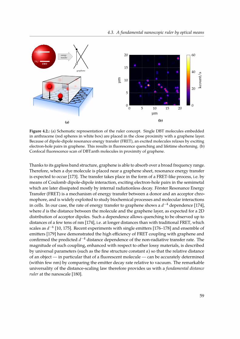
4.3. A fundamental nanoscopic ruler by optical means
|S0〉DBT
|S1〉
graphene
energytransfer
(a)
0 5 10 15 200
5
10
15
20
µmµm
0
20
40
60
kcou
nt/s
(b)
Figure 4.2.: (a) Schematic representation of the ruler concept. Single DBT molecules embeddedin anthracene (red spheres in white box) are placed in the close proximity with a graphene layer.Because of dipole-dipole resonance energy transfer (FRET), an excited molecules relaxes by excitingelectron-hole pairs in graphene. This results in fluorescence quenching and lifetime shortening. (b)Confocal fluorescence scan of DBT:anth molecules in proximity of graphene.
Thanks to its gapless band structure, graphene is able to absorb over a broad frequency range.Therefore, when a dye molecule is placed near a graphene sheet, resonance energy transferis expected to occur [173]. The transfer takes place in the form of a FRET-like process, i.e. bymeans of Coulomb dipole-dipole interaction, exciting electron-hole pairs in the semimetalwhich are later dissipated mostly by internal radiationless decay. Förster Resonance EnergyTransfer (FRET) is a mechanism of energy transfer between a donor and an acceptor chro-mophore, and is widely exploited to study biochemical processes and molecular interactionsin cells. In our case, the rate of energy transfer to graphene shows a d−4 dependence [174],where d is the distance between the molecule and the graphene layer, as expected for a 2Ddistribution of acceptor dipoles. Such a dependence allows quenching to be observed up todistances of a few tens of nm [174], i.e. at longer distances than with traditional FRET, whichscales as d−6 [10, 175]. Recent experiments with single emitters [176–178] and ensemble ofemitters [179] have demonstrated the high efficiency of FRET coupling with graphene andconfirmed the predicted d−4 distance dependence of the non-radiative transfer rate. Themagnitude of such coupling, enhanced with respect to other lossy materials, is describedby universal parameters (such as the fine structure constant α) so that the relative distanceof an object — in particular that of a fluorescent molecule — can be accurately determined(within few nm) by comparing the emitter decay rate relative to vacuum. The remarkableuniversality of the distance-scaling law therefore provides us with a fundamental distanceruler at the nanoscale [180].
59

Chapter 4. Proof of principle for a graphene-based nanoscopic ruler
In the near-field range, plasmonic rulers have been proposed [181, 182] and employedto measure nuclease activity [183], to follow dimer assembly and DNA hybridization [184].In the simplest geometry, two metal nano particles, integrated into the sample as a probe,interact with each other, yielding a shift of the plasmonic resonance which obeys a 1/d3
distance dependence. Different schemes helped improving sensitivity (up to about 10–15 nm)or maximum range (40 nm [185]), by means of nanoparticle-induced lifetime modification.The promise of plasmonic rulers, however, has been partially compromised by a lack ofuniversality, as the actual scaling laws typically depend on the nano-particle shape [186].The work that we present in this chapter represents a key extension of another ruler species,based on FRET [10, 152, 187], which may be employed to measure distances beyond 10 nm.More specifically, our method relies on the efficient coupling between single DBT moleculesand a graphene monolayer.
A schematic viewof our proof of concept for a graphene nanoruler is depicted in figure 4.2a.Single DBT molecules embedded in an anthracene crystal are brought in close proximitywith a one-atom-thick sheet of undoped graphene. Considering the typical thickness ofthe anthracene crystals (section 3.2.1) we are always working in the limit where d < λ/4;furthermore, since we are using undoped graphene, coupling to surface plasmons is notpossible so that the main relaxation mechanism in our configuration is FRET-like. DifferentDBT molecules, embedded at different depths inside the crystal, will exhibit differentdegrees of coupling. The otherwise almost unitary quantum yield defined by equation (2.1)is quenched by the onset of the new nonradiative decay channel:
φF =Γrad
Γrad + Γnrad(4.1)
Fluorescence lifetime (equation 2.4) is also strongly reduced, since the Förster-like transfertakes place on time scales that are shorter than the radiative lifetime (τnrad < τrad):
1τF
=1
τrad+
1τnrad
(4.2)
In the following, we perform a full statistical survey on the lifetimes of single DBT moleculesshowing the effect of coupling to graphene. At the single emitter level, a quantitative analysisfor the decay rate modification was still missing to date.
4.4. A single graphene layer
The graphene monolayers under investigation have been fabricated by chemical vapour de-position (CVD) on copper [188]. Polycrystalline graphene is then transferred on amicroscopeslide and annealed in H2-Ar (1:5) at 300 C for 3 hours. Later, anthracene crystals contain-ing single DBT molecules are spin-casted on the same coverslide following the proceduredescribed in section 3.2.1.
60

4.4. A single graphene layer
1 500 1 600 1 700 1 800 1 900 2 000 2 100 2 200 2 300 2 400 2 500 2 600 2 700 2 800
G 2D
Raman shift (cm−1)
Inte
nsity
(a.u
.)
Figure 4.3.: Raman spectrum of the CVD pristine graphene sample, obtained with a CW solid statediode laser (640 nm), exhibiting the characteristic lines at ≈ 1581 cm−1 and ≈ 2640 cm−1. The singleLorentzian profile of the 2D band, the respective positions and relative amplitude for G and 2Dbands show unambiguously a signature of a graphene monolayer.
Prior to the spincoating of DBT:anth crystals, we verify the presence of a single graphenelayer by performing Raman spectroscopy on the sample. Across graphene-related research,Raman spectroscopy is the preferred tool to investigate doping, stress and structural proper-ties [189]. Indeed, it is a fast and non-invasive technique allowing unambiguous identificationof graphene layers and their properties. Electron-phonon scattering processes involvingneighbouring Dirac cones give rise to characteristic Raman lines, providing information onboth electron and phonon bands. In particular, a clear signature for single layer graphenewould be the observation of the G peak at ≈ 1580 cm−1 and the 2D (also known as G′) bandat ≈ 2700 cm−1 [190]. The G band originates from one-phonon processes involving thedoubly degenerate phononmode E2g at the centre of the Brillouin zone. The 2D peak insteadoriginates from a two-phonon scattering process. In a single layer of graphene, the 2D peakis roughly four times more intense than the G peak and has a narrow shape [190]. For anincreasing number of layers, the 2D band is up-shifted and becomes broader, consisting ofmultiple components.The experimental setup that we use is the standard configuration for confocal Raman
spectroscopy. We employ a 100X objective with NA= 0.7 and excite the sample using acontinuous wave solid state diode laser, with central emission wavelength around 640 nmand TEM00 spatial mode. A narrow (2 nm) bandpass filter is used in excitation to clean thelaser beam, whereas a longpass filter in the detection path only lets the Stokes shifted lightthrough, while filtering out Rayleigh scattered light. Finally, the Raman spectra are collectedwith a grating spectrometer with a spectral resolution of 3 cm−1.
Figure 4.3 shows the measured Raman spectrum of a graphene specimen prepared asdescribed above. The two prominent features of a graphene monolayer can be readilyidentified, i.e. the G and 2D bands. The G band position is measured at 1581 cm−1 and has
61

Chapter 4. Proof of principle for a graphene-based nanoscopic ruler
0 2 4 6 8 10 12
0.1
1
t (ns)
Norm.inten
sity
(cou
nts/
s)τA = 1.6 nsτB = 4.0 nsfitIRF
0
0.2
0.4
0.6
0.8
1
arb.
units
Figure 4.4.: Time-resolved measurements of the fluorescence decay for single DBT:anth molecules,situated at different distances from a graphene layer. Solid black lines are fit to the experimentaldata with the convolution between the Instrument Response Function (IRF) (light grey) and a single-exponential-decay. The longer lifetime of molecule B compared to A is associated to a brighter signal,as displayed on the right in the close-up of a bigger confocal fluorescence scan. The quenching offluorescence and the shortening of its lifetime suggest that molecule A sits closer to graphene thanmolecule B.
pure Lorentzian shape. The profile of the Raman 2D band at 2640 cm−1 is Lorentzian andshows correct agreement with the expected line shape for monolayer graphene [190, 191].The D band at≈ 1350 cm−1 —which is activated only in the presence of structural defects —is not observed, suggesting the purity of the sample.
4.5. Statistical survey of lifetime measurements
The decay rate of molecules coupled and uncoupled to graphene are compared in terms ofexcited-state lifetime measurements. The fluorescence dynamics are probed as described insection 3.3.5, using a pulsed Ti:sa laser and the PicoHarpmodule for TCSPC. We performthe analysis in a systematic way, starting from a scan similar to the one in figure 4.2b anddefining an intensity threshold for the faintest detectable molecule according to a minimumSNR of 3. On each selected molecule, we then measure the relaxation dynamics and extracta value for the excited-state lifetime. Figure 4.4a shows particularly clean single-exponentialdecays of DBT fluorescence in the vicinity of graphene. As anticipated in chapter 3, suchsignals can be associated to a single optically active system with a simple level structure, i.e.with no contribution from the host matrix [119].
In fitting the decay curves, we have to take into account that the excitation pulse is nota delta-function and that the instrumentation has a finite response time, quantified by theInstrument Response Function (IRF) or L(t), which can be determined by measuring theinstrument response profile to the backscattered laser light (grey solid line in figure 4.4a).
62

4.5. Statistical survey of lifetime measurements
(a) (b) (c)
Figure 4.5.: A graphene flake, seen through an optical microscope (a) can be imaged by observingthe fluorescence quenching (b) or lifetime shortening (c) of a layer of rhodamine molecules. Adaptedwith permission from L. Gaudreau et al. “Universal Distance-Scaling of Nonradiative Energy Transferto Graphene”. In: Nano Lett. 13, 5 (Mar. 2013), pp. 2030–2035. © 2013 American Chemical Society.
The IRF is approximately a Gaussian with σ ≈ 400 ns, corresponding mainly to the APD’sjitter. If we think L(t) as a series of delta-excitation pulses with varying amplitude, thenthe measured intensity at time t, N(t), is the convolution integral between L(t) and thefluorescence intensity I(t) from the emitter:
N(t) =∫ t
0L(t′)I(t− t′)dt′ (4.3)
In fitting the decay curves we account for the IRF by employing DecayFit, a fluorescencedecay analysis software based on MATLAB [192]. In the fitting procedure no actual de-convolution takes place; rather, iterative reconvolution is implemented, i.e. decay times arederived from the best fit of the convolution between the IRF and a single-exponential decaymodel.The proximity to a graphene monolayer is clearly reflected in lifetime measurements: a
molecule, say molecule A in the example shown in figure 4.4, is characterized by a shortlifetime due to efficient energy transfer to the graphene sheet, also resulting in fluorescencequenching. On the other hand, molecule B appears brighter and with a longer lifetime, andis supposedly further away from the graphene layer compared to the other molecule. Aswe have anticipated, shorter lifetimes are due to the non-radiative decay rate enhancement,which results in a decreased quantum efficiency (equation 4.1), and lifetime shortening(equation 4.2). Fluorescence quenching [176, 179, 193] or even lifetime mapping [176, 179]can be exploited to image a graphene monolayer (figure 4.5), or to characterize the couplingefficiency between emitters and graphene [177].
As a reference test sample we consider our usual DBT:anth crystals spincoated on a bareSiO2 coverslide, and collect lifetime measurements for 75 molecules. In the histogram shownin figure 4.6a we observe a symmetric distribution of lifetimes around 4.1 ns with σ ' 0.4 ns,
63
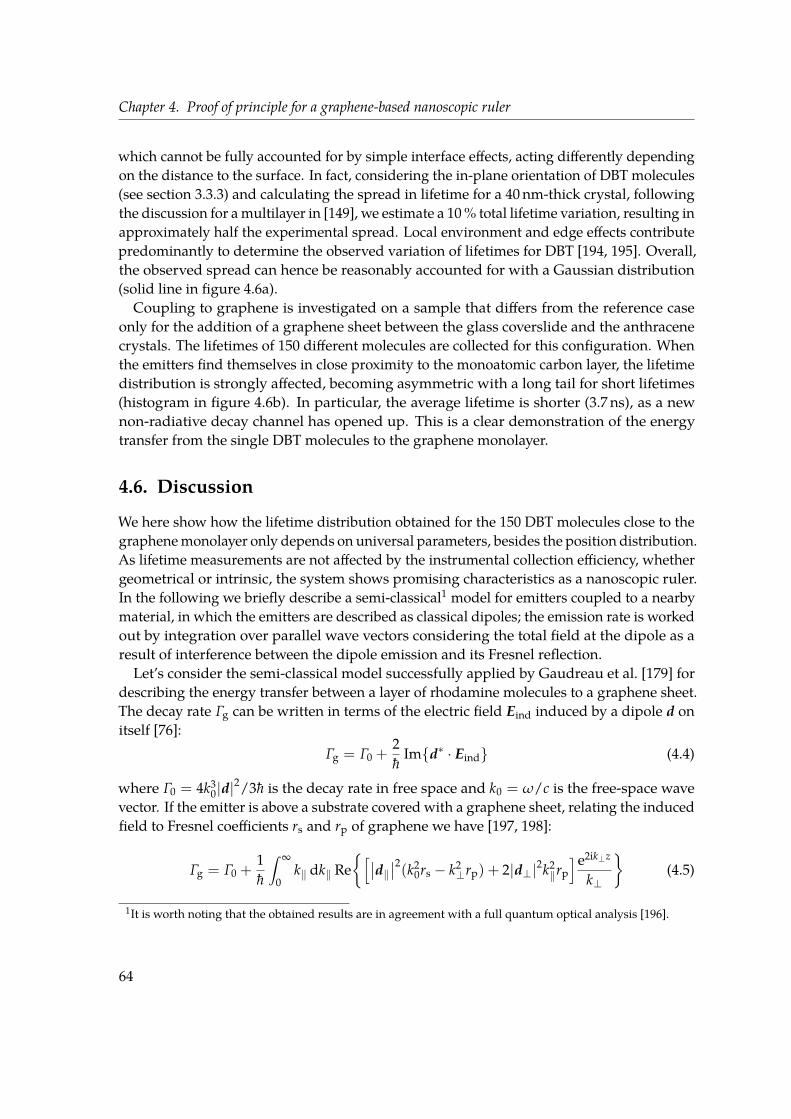
Chapter 4. Proof of principle for a graphene-based nanoscopic ruler
which cannot be fully accounted for by simple interface effects, acting differently dependingon the distance to the surface. In fact, considering the in-plane orientation of DBT molecules(see section 3.3.3) and calculating the spread in lifetime for a 40 nm-thick crystal, followingthe discussion for amultilayer in [149], we estimate a 10% total lifetime variation, resulting inapproximately half the experimental spread. Local environment and edge effects contributepredominantly to determine the observed variation of lifetimes for DBT [194, 195]. Overall,the observed spread can hence be reasonably accounted for with a Gaussian distribution(solid line in figure 4.6a).
Coupling to graphene is investigated on a sample that differs from the reference caseonly for the addition of a graphene sheet between the glass coverslide and the anthracenecrystals. The lifetimes of 150 different molecules are collected for this configuration. Whenthe emitters find themselves in close proximity to the monoatomic carbon layer, the lifetimedistribution is strongly affected, becoming asymmetric with a long tail for short lifetimes(histogram in figure 4.6b). In particular, the average lifetime is shorter (3.7 ns), as a newnon-radiative decay channel has opened up. This is a clear demonstration of the energytransfer from the single DBT molecules to the graphene monolayer.
4.6. Discussion
We here show how the lifetime distribution obtained for the 150 DBT molecules close to thegraphenemonolayer only depends on universal parameters, besides the position distribution.As lifetime measurements are not affected by the instrumental collection efficiency, whethergeometrical or intrinsic, the system shows promising characteristics as a nanoscopic ruler.In the following we briefly describe a semi-classical1 model for emitters coupled to a nearbymaterial, in which the emitters are described as classical dipoles; the emission rate is workedout by integration over parallel wave vectors considering the total field at the dipole as aresult of interference between the dipole emission and its Fresnel reflection.Let’s consider the semi-classical model successfully applied by Gaudreau et al. [179] for
describing the energy transfer between a layer of rhodamine molecules to a graphene sheet.The decay rate Γg can be written in terms of the electric field Eind induced by a dipole d onitself [76]:
Γg = Γ0 +2h
Imd∗ · Eind (4.4)
where Γ0 = 4k30|d|2/3h is the decay rate in free space and k0 = ω/c is the free-space wave
vector. If the emitter is above a substrate covered with a graphene sheet, relating the inducedfield to Fresnel coefficients rs and rp of graphene we have [197, 198]:
Γg = Γ0 +1h
∫ ∞
0k‖ dk‖ Re
[∣∣d‖∣∣2(k2
0rs − k2⊥rp) + 2|d⊥|2k2
‖rp]e2ik⊥z
k⊥
(4.5)
1It is worth noting that the obtained results are in agreement with a full quantum optical analysis [196].
64

4.6. Discussion
1 2 3 4 50
0.5
1
1.5
τ (ns)
P(τ)
experimentGaussian
(a)
1 2 3 4 50
0.2
0.4
0.6
0.8
τ (ns)P(τ)
experimentmodel
(b)
0 20 40 60 800
1
2
·10−2
d (nm)
P(d)
(c)
0 10 20 300
5
10
d (nm)
∆d
(nm
)
(d)
Figure 4.6.: Probability Density Function (PDF) of the excited state lifetimes of single DBT:anthmolecules on a bare glass substrate (a) and on the same substrate with an added graphene sheet (b).Histograms represent experimental values, while blue solid lines result from the theoretical modelsdiscussed in the text. The bin size is given by the time resolution of the setup, amounting to 400 psafter deconvolution with the instrument response function. A PDF of a normal distribution (solidline), centred around 4.2 ns is used to reproduce the intrinsic spread in lifetimes of DBT molecules ina thin anthracene film. The PDF for lifetimes on graphene is obtained from the model by assumingthe Gaussian distribution of panel (a) for the lifetimes in the uncoupled case, and the PDF reportedin panel (c) for the molecule-graphene distances. The expected potential accuracy in operating oursystem to measure distances is plotted in panel (d) as a function of the relative distance.
65

Chapter 4. Proof of principle for a graphene-based nanoscopic ruler
where z is the emitter-graphene distance and the integral is computed over wave vectorsparallel to graphene (k‖). In the long wavelength limit, i.e. for small distances compared tothe emission wavelength, we obtain:
Γg ≈ Γ0 +1h(∣∣d‖∣∣2 + 2|d⊥|2)
∫ ∞
0k2‖ dk‖ Im
rp
e−2k‖z (4.6)
from which the ratio of decay rates is written as [179]:
Γg
Γ0= 1 +
3νλ30
32π3
∫ ∞
0k2‖ dk‖ Im
rp
e−2k‖z (4.7)
where λ0 is the light wavelength and ν = 1 (ν = 2) when the dipole is oriented parallel(perpendicular) to the surface. The k‖ dependence of the Fresnel coefficient is at the originof the distance dependence of decay rate. For graphene, we have
Im
rp= Im
−2
ε + 1 + 4πiσk‖/ω
(4.8)
where σ is the graphene conductivity, ω the photon frequency and ε the permittivity of thesubstrate supporting graphene. By taking σ = e2/4h, the above integral has a closed-formanalytical solution written as Γg/Γ0 = 1+ νCI(x)where C = 3(ε + 1)2/2(πα)3 is a constant,x = 4(ε + 1)d/αλ0 and I(x) ≈ 1/(x2 + x3/3 + x4/6). In the distance range of interest forour work, the solution reduces to a simple elegant formula:
Γg
Γ0≈ 1 +
9να
256π3(ε + 1)2
(λ0
d
)4
(4.9)
having the well-known d−4 dependence. In the formula above, d is the sole unknown, theother quantities being universal constants, the substrate permittivity and the wavelength.There are no material-dependent parameters related to graphene. The universality of thismodel lies in the universal value of the optical conductivity that we used, which in turnderives from graphene’s pure 2D structure and gapless band structure.We now go back to our case of single DBT molecules in anthracene in close proximity
to a graphene layer. The effect of energy transfer to graphene is compared to the referencecase of DBT:anth molecules on the substrate without graphene. To keep the model simple,we consider the DBT molecules as embedded in a semi-infinite anthracene medium, wherethe lifetimes of DBT molecules are characterized by the homogeneous (phenomenological)Gaussian distribution as shown in figure 4.6a. This assumption is motivated by theoreticalcalculations according to which the finite-size effect of the anthracene crystal on the emitterlifetime spread is of secondary importance compared to local-field and edge effects [149].We thus find the following simple model to be effective in describing the energy transferbetween single DBT molecules and a graphene sheet:
Γg
Γng≈ 1 +
9α
256π3(εsub + εanthr)2
(λ0
d
)4
(4.10)
66
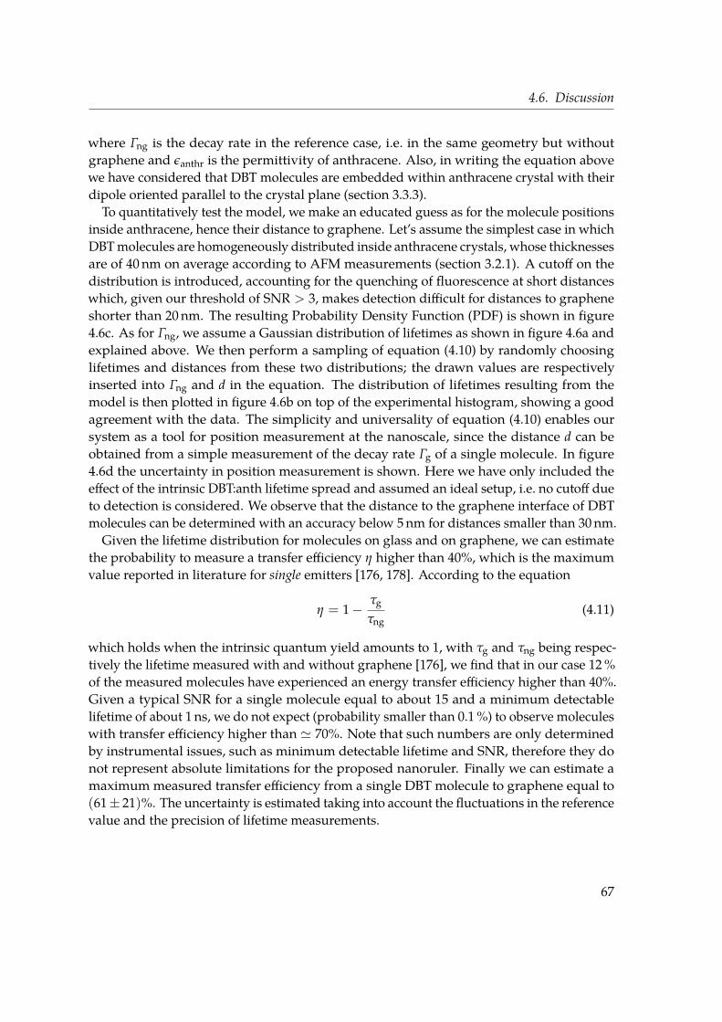
4.6. Discussion
where Γng is the decay rate in the reference case, i.e. in the same geometry but withoutgraphene and εanthr is the permittivity of anthracene. Also, in writing the equation abovewe have considered that DBT molecules are embedded within anthracene crystal with theirdipole oriented parallel to the crystal plane (section 3.3.3).
To quantitatively test the model, we make an educated guess as for the molecule positionsinside anthracene, hence their distance to graphene. Let’s assume the simplest case in whichDBTmolecules are homogeneously distributed inside anthracene crystals, whose thicknessesare of 40 nm on average according to AFM measurements (section 3.2.1). A cutoff on thedistribution is introduced, accounting for the quenching of fluorescence at short distanceswhich, given our threshold of SNR > 3, makes detection difficult for distances to grapheneshorter than 20 nm. The resulting Probability Density Function (PDF) is shown in figure4.6c. As for Γng, we assume a Gaussian distribution of lifetimes as shown in figure 4.6a andexplained above. We then perform a sampling of equation (4.10) by randomly choosinglifetimes and distances from these two distributions; the drawn values are respectivelyinserted into Γng and d in the equation. The distribution of lifetimes resulting from themodel is then plotted in figure 4.6b on top of the experimental histogram, showing a goodagreement with the data. The simplicity and universality of equation (4.10) enables oursystem as a tool for position measurement at the nanoscale, since the distance d can beobtained from a simple measurement of the decay rate Γg of a single molecule. In figure4.6d the uncertainty in position measurement is shown. Here we have only included theeffect of the intrinsic DBT:anth lifetime spread and assumed an ideal setup, i.e. no cutoff dueto detection is considered. We observe that the distance to the graphene interface of DBTmolecules can be determined with an accuracy below 5nm for distances smaller than 30 nm.Given the lifetime distribution for molecules on glass and on graphene, we can estimate
the probability to measure a transfer efficiency η higher than 40%, which is the maximumvalue reported in literature for single emitters [176, 178]. According to the equation
η = 1− τg
τng(4.11)
which holds when the intrinsic quantum yield amounts to 1, with τg and τng being respec-tively the lifetime measured with and without graphene [176], we find that in our case 12%of the measured molecules have experienced an energy transfer efficiency higher than 40%.Given a typical SNR for a single molecule equal to about 15 and a minimum detectablelifetime of about 1 ns, we do not expect (probability smaller than 0.1%) to observe moleculeswith transfer efficiency higher than ' 70%. Note that such numbers are only determinedby instrumental issues, such as minimum detectable lifetime and SNR, therefore they donot represent absolute limitations for the proposed nanoruler. Finally we can estimate amaximum measured transfer efficiency from a single DBT molecule to graphene equal to(61± 21)%. The uncertainty is estimated taking into account the fluctuations in the referencevalue and the precision of lifetime measurements.
67

Chapter 4. Proof of principle for a graphene-based nanoscopic ruler
4.7. Conclusions
In conclusion, we have presented a full statistical study of the coupling between singlelong-lived organic molecules and a graphene monolayer sheet. We have reported the highest— to our knowledge — ever measured transfer efficiency from single emitters to graphene,amounting to 61± 21%. The molecule excited-state lifetime is strongly affected by the pres-ence of the monoatomic carbon layer, because of its two-dimensionality, high conductivityand gapless dispersion relation. As a result, we can detect a FRET-like effect to distanceswell beyond the characteristic range of 10 nm of standard acceptor-donor energy transfer.The semi-classical model yielding a universal d−4 dependence of the coupling efficiency[179, 180] was successfully verified in the near-field range against a statistical distribution ofthe molecule lifetimes. The presented investigation on our favourable DBT:anth platformconstitutes a proof of principle for a graphene-based nano ruler, where ideally the distanceto a surface can be measured by extracting the lifetime of a well-referenced single emitter,serving as a marker. We expect a N-fold increase of the effect for a N-layer system becausethe optical conductivity (and thus the energy transfer rate) increases linearly with N for atleast up to 5 layers [199].
In the near future, the use of single emitters will be essential to focus on local effects suchas mapping the local Fermi energy in graphene, useful for electron-transport engineering ingraphene-based devices. Dibenzoterrylene molecules, emitting single photons on demandin the near infrared, are also particularly promising candidates to launch deterministicsingle plasmons into heavily-doped graphene. Recently, new hybrid electro-optomechanicalsystems exploiting the excellent mechanical properties of graphene have been proposed, inwhich the strength of coupling between single quantum emitters and a graphene resonatoris controlled by the electrostatic deflection of a suspended graphene membrane [200]. In asimilar geometry, quantum emitters such as our DBT:anth system could be used in anotherkind of conceptual nanorulers, based on the Casimir interaction with a surface such asgraphene or MoS2. In this case, the physical mechanism on which the ruler is based is themodification of the energy of the emitter’s electronic states — hence its transition frequency— due to the vacuum fluctuations in the presence of a nearby surface [201]. The field ofquantum sensing is today a very thriving one, and new interesting applications are to beexpected in the coming years.
68

References
[1] M. Fox. Quantum Optics: An Introduction. 6. Oxford university press, 2006.[2] B. Lounis, H. Bechtel, D. Gerion, P. Alivisatos, andW.Moerner. “Photon antibunching
in single CdSe/ZnS quantum dot fluorescence”. In: Chemical Physics Letters 329, 5(2000), pp. 399–404.
[3] R. Verberk and M. Orrit. “Photon statistics in the fluorescence of single moleculesand nanocrystals: Correlation functions versus distributions of on-and off-times”. In:The Journal of Chemical Physics 119, 4 (2003), pp. 2214–2222.
[4] B. Lounis and M. Orrit. “Single-photon sources”. In: Reports on Progress in Physics 68,5 (2005), p. 1129.
[5] S. Singh. “Antibunching, sub-poissonian photon statistics and finite bandwidtheffects in resonance fluorescence”. In: Optics Communications 44, 4 (1983), pp. 254–258.
[6] X. Zou and L. Mandel. “Photon-antibunching and sub-Poissonian photon statistics”.In: Phys. Rev. A 41, 1 (1990), p. 475.
[7] R. Hanbury Brown and R. Q. Twiss. “Correlation between photons in two coherentbeams of light”. In: Nature 177 (1956), pp. 27–29.
[8] H. Kimble, M. Dagenais, and L. Mandel. “Photon antibunching in resonance fluores-cence”. In: Phys. Rev. Lett. 39, 11 (1977), p. 691.
[9] T. Basché, W. Moerner, M. Orrit, and H. Talon. “Photon antibunching in the fluores-cence of a single dye molecule trapped in a solid”. In: Phys. Rev. Lett. 69, 10 (1992),p. 1516.
[10] J. R. Lakowicz. Principles of Fluorescence Spectroscopy. Springer, 2006.[11] M. Wahl. Time-Correlated Single Photon Counting. PicoQuant Technical Note.[12] J. F. Clauser. “Experimental distinction between the quantum and classical field-
theoretic predictions for the photoelectric effect”. In: Phys. Rev. D 9, 4 (1974), p. 853.[13] A. Aspect, P. Grangier, and G. Roger. “Experimental tests of realistic local theories
via Bell’s theorem”. In: Phys. Rev. Lett. 47, 7 (1981), p. 460.[14] P. Grangier, G. Roger, and A. Aspect. “Experimental evidence for a photon anticorre-
lation effect on a beam splitter: a new light on single-photon interferences”. In: EPL(Europhysics Letters) 1, 4 (1986), p. 173.
69

References
[15] F. Diedrich and H. Walther. “Nonclassical radiation of a single stored ion”. In: Phys.Rev. Lett. 58, 3 (1987), p. 203.
[16] C. Hong and L. Mandel. “Experimental realization of a localized one-photon state”.In: Phys. Rev. Lett. 56, 1 (1986), p. 58.
[17] J. Beugnon, M. P. Jones, J. Dingjan, B. Darquié, G. Messin, A. Browaeys, and P. Grang-ier. “Quantum interference between two single photons emitted by independentlytrapped atoms”. In: Nature 440, 7085 (2006), pp. 779–782.
[18] P. Maunz, D. Moehring, S. Olmschenk, K. Younge, D. Matsukevich, and C. Monroe.“Quantum interference of photon pairs from two remote trapped atomic ions”. In:Nature Physics 3, 8 (2007), pp. 538–541.
[19] B. Lounis and W. Moerner. “Single photons on demand from a single molecule atroom temperature”. In: Nature 407, 6803 (2000), pp. 491–493.
[20] N. Bar-Gill, L. Pham, C. Belthangady, D. Le Sage, P. Cappellaro, J. Maze, M. Lukin,A. Yacoby, and R. Walsworth. “Suppression of spin-bath dynamics for improvedcoherence of multi-spin-qubit systems”. In: Nature Communications 3 (2012), p. 858.
[21] G. Juska, V. Dimastrodonato, L. O. Mereni, A. Gocalinska, and E. Pelucchi. “Towardsquantum-dot arrays of entangled photon emitters”. In: Nature Photonics 7, 7 (2013),pp. 527–531.
[22] A. Gruber, A. Dräbenstedt, C. Tietz, L. Fleury, J. Wrachtrup, and C. Von Borczysko-wski. “Scanning confocal optical microscopy andmagnetic resonance on single defectcenters”. In: Science 276, 5321 (1997), pp. 2012–2014.
[23] C. Kurtsiefer, S. Mayer, P. Zarda, and H. Weinfurter. “Stable solid-state source ofsingle photons”. In: Phys. Rev. Lett. 85, 2 (2000), p. 290.
[24] R. Brouri, A. Beveratos, J.-P. Poizat, and P. Grangier. “Photon antibunching in thefluorescence of individual color centers in diamond”. In: Optics Letters 25, 17 (2000),pp. 1294–1296.
[25] F. Jelezko, T. Gaebel, I. Popa, M. Domhan, A. Gruber, and J. Wrachtrup. “Observa-tion of coherent oscillation of a single nuclear spin and realization of a two-qubitconditional quantum gate”. In: Phys. Rev. Lett. 93, 13 (2004), p. 130501.
[26] P. Neumann, R. Kolesov, B. Naydenov, J. Beck, F. Rempp, M. Steiner, V. Jacques,G. Balasubramanian, M. Markham, D. Twitchen, et al. “Quantum register based oncoupled electron spins in a room-temperature solid”. In: Nature Physics 6, 4 (2010),pp. 249–253.
[27] F. Jelezko, C. Tietz, A. Gruber, I. Popa, A. Nizovtsev, S. Kilin, and J. Wrachtrup.“Spectroscopy of single NV centers in diamond”. In: Single Molecules 2, 4 (2001),pp. 255–260.
70

References
[28] A. Beveratos, R. Brouri, T. Gacoin, J.-P. Poizat, and P. Grangier. “Nonclassical radiationfrom diamond nanocrystals”. In: Phys. Rev. A 64, 6 (2001), p. 061802.
[29] J. Rabeau, A. Stacey, A. Rabeau, S. Prawer, F. Jelezko, I. Mirza, and J. Wrachtrup.“Single nitrogen vacancy centers in chemical vapor deposited diamond nanocrystals”.In: Nano letters 7, 11 (2007), pp. 3433–3437.
[30] M. W. Doherty, N. B. Manson, P. Delaney, F. Jelezko, J. Wrachtrup, and L. C. Hol-lenberg. “The nitrogen-vacancy colour centre in diamond”. In: Physics Reports 528, 1(2013), pp. 1–45.
[31] C. Wang, C. Kurtsiefer, H. Weinfurter, and B. Burchard. “Single photon emissionfrom SiV centres in diamond produced by ion implantation”. In: Journal of Physics B:Atomic, Molecular and Optical Physics 39, 1 (2006), p. 37.
[32] E. Neu, D. Steinmetz, J. Riedrich-Möller, S. Gsell, M. Fischer, M. Schreck, and C.Becher. “Single photon emission from silicon-vacancy colour centres in chemicalvapour deposition nano-diamonds on iridium”. In:New Journal of Physics 13, 2 (2011),p. 025012.
[33] E. Neu, M. Agio, and C. Becher. “Photophysics of single silicon vacancy centers indiamond: implications for single photon emission”. In: Optics Express 20, 18 (2012),pp. 19956–19971.
[34] M.Abbarchi, F. Troiani, C.Mastrandrea, G. Goldoni, T. Kuroda, T.Mano, K. Sakoda, N.Koguchi, S. Sanguinetti, A. Vinattieri, et al. “Spectral diffusion and line broadening insingle self-assembled GaAs/ AlGaAs quantum dot photoluminescence”. In: AppliedPhysics Letters 93, 16 (2008), p. 162101.
[35] M. Orrit and T. Basché. “Steady light from quantum dots, at last. But how?” In:ChemPhysChem 10, 14 (2009), pp. 2383–2385.
[36] M. J. Fernée, T. Plakhotnik, Y. Louyer, B. N. Littleton, C. Potzner, P. Tamarat, P.Mulvaney, and B. Lounis. “Spontaneous spectral diffusion in CdSe quantum dots”.In: The Journal of Physical Chemistry Letters 3, 12 (2012), pp. 1716–1720.
[37] P. Michler, A. Imamoğlu, M. Mason, P. Carson, G. Strouse, and S. Buratto. “Quantumcorrelation among photons from a single quantum dot at room temperature”. In:Nature 406, 6799 (2000), pp. 968–970.
[38] S. Buckley, K. Rivoire, and J. Vučković. “Engineered quantum dot single-photonsources”. In: Reports on Progress in Physics 75, 12 (2012), p. 126503.
[39] J. Rarity, P. Owens, and P. Tapster. “Quantum random-number generation and keysharing”. In: Journal of Modern Optics 41, 12 (1994), pp. 2435–2444.
[40] M. Wahl, M. Leifgen, M. Berlin, T. Röhlicke, H.-J. Rahn, and O. Benson. “An ultrafastquantum random number generator with provably bounded output bias based onphoton arrival time measurements”. In:Applied Physics Letters 98, 17 (2011), p. 171105.
71

References
[41] T. D. Ladd, F. Jelezko, R. Laflamme, Y. Nakamura, C. Monroe, and J. L. O’Brien.“Quantum computers”. In: Nature 464, 7285 (2010), pp. 45–53.
[42] H. J. Kimble. “The quantum internet”. In: Nature 453, 7198 (2008), pp. 1023–1030.[43] E. Knill, R. Laflamme, and G. J. Milburn. “A scheme for efficient quantum computa-
tion with linear optics”. In: Nature 409, 6816 (2001), pp. 46–52.[44] T. Sleator and H. Weinfurter. “Realizable universal quantum logic gates”. In: Phys.
Rev. Lett. 74, 20 (1995), p. 4087.[45] C. Hong, Z. Ou, and L. Mandel. “Measurement of subpicosecond time intervals
between two photons by interference”. In: Phys. Rev. Lett. 59, 18 (1987), p. 2044.[46] P. Grangier. “Quantum physics: Single photons stick together”. In: Nature 419, 6907
(2002), pp. 577–577.[47] C. Santori, D. Fattal, J. Vučković, G. S. Solomon, and Y. Yamamoto. “Indistinguishable
photons from a single-photon device”. In: Nature 419, 6907 (2002), pp. 594–597.[48] M. Leifgen, T. Schröder, F. Gädeke, R. Riemann, V. Métillon, E. Neu, C. Hepp, C.
Arend, C. Becher, K. Lauritsen, and O. Benson. “Evaluation of nitrogen-and silicon-vacancy defect centres as single photon sources in quantum key distribution”. In:New Journal of Physics 16, 2 (2014), p. 023021.
[49] J. I. Cirac, P. Zoller, H. J. Kimble, and H. Mabuchi. “Quantum state transfer andentanglement distribution among distant nodes in a quantum network”. In: Phys.Rev. Lett. 78, 16 (1997), p. 3221.
[50] X. Maitre, E. Hagley, G. Nogues, C. Wunderlich, P. Goy, M. Brune, J. Raimond, andS. Haroche. “Quantum memory with a single photon in a cavity”. In: Phys. Rev. Lett.79, 4 (1997), p. 769.
[51] S. Brattke, B. T. Varcoe, and H. Walther. “Generation of photon number states on de-mand via cavity quantum electrodynamics”. In: Phys. Rev. Lett. 86, 16 (2001), p. 3534.
[52] A. Kuhn, M. Hennrich, and G. Rempe. “Deterministic single-photon source for dis-tributed quantum networking”. In: Phys. Rev. Lett. 89, 6 (2002), p. 067901.
[53] J. McKeever, A. Boca, A. Boozer, R. Miller, J. Buck, A. Kuzmich, and H. Kimble.“Deterministic generation of single photons from one atom trapped in a cavity”. In:Science 303, 5666 (2004), pp. 1992–1994.
[54] T. Wilk, S. C. Webster, A. Kuhn, and G. Rempe. “Single-atom single-photon quantuminterface”. In: Science 317, 5837 (2007), pp. 488–490.
[55] S. Ritter, C. Nölleke, C. Hahn, A. Reiserer, A. Neuzner, M. Uphoff, M. Mücke, E.Figueroa, J. Bochmann, and G. Rempe. “An elementary quantum network of singleatoms in optical cavities”. In: Nature 484, 7393 (2012), pp. 195–200.
[56] T. Northup and R. Blatt. “Quantum information transfer using photons”. In: NaturePhotonics 8, 5 (2014), pp. 356–363.
72

References
[57] D. E. Chang, V. Vuletić, andM. D. Lukin. “Quantum nonlinear optics [mdash] photonby photon”. In: Nature Photonics 8, 9 (2014), pp. 685–694.
[58] D. Englund, A. Faraon, I. Fushman, N. Stoltz, P. Petroff, and J. Vučković. “Controllingcavity reflectivity with a single quantum dot”. In: Nature 450, 7171 (2007), pp. 857–861.
[59] D. Englund, A. Faraon, B. Zhang, Y. Yamamoto, and J. Vučković. “Generation andtransfer of single photons on a photonic crystal chip”. In: Optics Express 15, 9 (2007),pp. 5550–5558.
[60] D. Press, S. Götzinger, S. Reitzenstein, C. Hofmann, A. Löffler, M. Kamp, A. Forchel,and Y. Yamamoto. “Photon antibunching from a single quantum-dot-microcavitysystem in the strong coupling regime”. In: Phys. Rev. Lett. 98, 11 (2007), p. 117402.
[61] I. Fushman, D. Englund, A. Faraon, N. Stoltz, P. Petroff, and J. Vučković. “Controlledphase shifts with a single quantum dot”. In: Science 320, 5877 (2008), pp. 769–772.
[62] A. Faraon, I. Fushman, D. Englund, N. Stoltz, P. Petroff, and J. Vučković. “Coher-ent generation of non-classical light on a chip via photon-induced tunnelling andblockade”. In: Nature Physics 4, 11 (2008), pp. 859–863.
[63] A. Faraon, A. Majumdar, D. Englund, E. Kim, M. Bajcsy, and J. Vučković. “Integratedquantum optical networks based on quantum dots and photonic crystals”. In: NewJournal of Physics 13, 5 (2011), p. 055025.
[64] J. Hwang and E. Hinds. “Dye molecules as single-photon sources and large opticalnonlinearities on a chip”. In: New Journal of Physics 13, 8 (2011), p. 085009.
[65] A. Reinhard, T. Volz, M. Winger, A. Badolato, K. J. Hennessy, E. L. Hu, and A. Ima-moğlu. “Strongly correlated photons on a chip”. In: Nature Photonics 6, 2 (2012),pp. 93–96.
[66] H. Kim, R. Bose, T. C. Shen, G. S. Solomon, and E. Waks. “A quantum logic gatebetween a solid-state quantum bit and a photon”. In: Nature Photonics 7, 5 (2013),pp. 373–377.
[67] A. W. Schell, H. Takashima, S. Kamioka, Y. Oe, M. Fujiwara, O. Benson, and S. Take-uchi. “Highly Efficient Coupling of Nanolight Emitters to a Ultra-Wide TunableNanofibre Cavity”. In: Scientific Reports 5 (2015).
[68] P. M. Vora, A. S. Bracker, S. G. Carter, T. M. Sweeney, M. Kim, C. S. Kim, L. Yang,P. G. Brereton, S. E. Economou, and D. Gammon. “Spin-cavity interactions betweena quantum dot molecule and a photonic crystal cavity”. In: Nature Communications 6(2015).
[69] A. Javadi, I. Sollner, M. Arcari, S. Lindskov Hansen, L. Midolo, S. Mahmoodian, G.Kirsanske, T. Pregnolato, E.H. Lee, J. D. Song, S. Stobbe, and P. Lodahl. “Single-photonnon-linear optics with a quantum dot in a waveguide”. In: Nature Communications 6(Oct. 2015).
73

References
[70] W. Moerner and L. Kador. “Optical detection and spectroscopy of single moleculesin a solid”. In: Phys. Rev. Lett. 62, 21 (1989), p. 2535.
[71] M. Orrit and J. Bernard. “Single pentacene molecules detected by fluorescence exci-tation in a p-terphenyl crystal”. In: Phys. Rev. Lett. 65, 21 (1990), p. 2716.
[72] Super-resolved fluorescence microscopy. Scientific Background on the Nobel Prize inChemistry 2014, compiled by the Class for Physics of the Royal Swedish Academy ofSciences. Oct. 2015.
[73] W. Moerner and M. Orrit. “Illuminating single molecules in condensed matter”. In:Science 283, 5408 (1999), pp. 1670–1676.
[74] P. Tamarat, B. Lounis, J. Bernard, M. Orrit, S. Kummer, R. Kettner, S. Mais, andT. Basché. “Pump-probe experiments with a single molecule: ac-stark effect andnonlinear optical response”. In: Phys. Rev. Lett. 75, 8 (1995), p. 1514.
[75] A. Jabłoński. “Efficiency of anti-Stokes fluorescence in dyes”. In: Nature 131, 839-840(1933), p. 21.
[76] L. Novotny and B. Hecht. Principles of nano-optics. Cambridge university press, 2012.[77] W. Moerner and D. P. Fromm. “Methods of single-molecule fluorescence spectro-
scopy and microscopy”. In: Review of Scientific Instruments 74, 8 (2003), pp. 3597–3619.
[78] W. Moerner, T. Plakhotnik, T. Irngartinger, M. Croci, V. Palm, and U. P. Wild. “OpticalProbing of Single Molecules of Terrylene in a Shpol’kii Matrix: A Two-State Single-Molecule Switch”. In: The Journal of Physical Chemistry 98, 30 (1994), pp. 7382–7389.
[79] T. Basché, S. Kummer, and C. Bräuchle. “Excitation and Emission Spectroscopy andQuantum Optical Measurements”. In: Single-molecule optical detection, imaging andspectroscopy. Ed. by W. Moerner, M. Orrit, U. Wild, and T. Basché. John Wiley & Sons,2008.
[80] R. Loudon. The quantum theory of light. Oxford university press, 2000.[81] F. Bloch. “Nuclear induction”. In: Physical Review 70, 7-8 (1946), p. 460.[82] T. Nonn and T. Plakhotnik. “Non-Lorentzian single-molecule line shape: Pseudolocal
phonons and coherence transfer”. In: Phys. Rev. Lett. 85, 7 (2000), p. 1556.[83] A. A. Nicolet, P. Bordat, C. Hofmann, M. A. Kol’chenko, B. Kozankiewicz, R. Brown,
and M. Orrit. “Single dibenzoterrylene molecules in an anthracene crystal: Maininsertion sites”. In: ChemPhysChem 8, 13 (2007), pp. 1929–1936.
[84] A. Brouwer, J. Köhler, E. Groenen, and J. Schmidt. “13C isotope effects for pentacenein p-terphenyl: High-resolution spectroscopy and single-spin detection”. In: TheJournal of Chemical Physics 105, 6 (1996), pp. 2212–2222.
[85] P. Tamarat, A. Maali, B. Lounis, and M. Orrit. “Ten years of single-molecule spec-troscopy”. In: The Journal of Physical Chemistry A 104, 1 (2000), pp. 1–16.
74

References
[86] Moerner, W.E. “Physical Principles and Methods of Single-Molecule Spectroscopyin Solids”. In: Single-molecule optical detection, imaging and spectroscopy. Ed. by W. Mo-erner, M. Orrit, U. Wild, and T. Basché. John Wiley & Sons, 2008.
[87] J.-M. Caruge and M. Orrit. “Investigations of local currents in a semiconductor bysingle-molecule spectroscopy”. In: Journal of Luminescence 98, 1 (2002), pp. 1–5.
[88] M. Kol’chenko, A. Nicolet, M. Galouzis, C. Hofmann, B. Kozankiewicz, and M. Orrit.“Single molecules detect ultra-slow oscillators in a molecular crystal excited by acvoltages”. In: New Journal of Physics 11, 2 (2009), p. 023037.
[89] S. Faez, S. J. van der Molen, and M. Orrit. “Optical tracing of multiple charges insingle-electron devices”. In: Phys. Rev. B 90, 20 (2014), p. 205405.
[90] Y. Tian, P. Navarro, and M. Orrit. “Single molecule as a local acoustic detector formechanical oscillators”. In: Phys. Rev. Lett. 113, 13 (2014), p. 135505.
[91] C. Hofmann, A. Nicolet, M. A. Kol’chenko, and M. Orrit. “Towards nanoprobesfor conduction in molecular crystals: Dibenzoterrylene in anthracene crystals”. In:Chemical physics 318, 1 (2005), pp. 1–6.
[92] A. A. L. Nicolet. “Single-molecule probes in organic field-effect transistors”. PhDthesis. 2007.
[93] L. Novotny and N. Van Hulst. “Antennas for light”. In: Nature Photonics 5, 2 (2011),pp. 83–90.
[94] M. Agio. Molecular scattering and fluorescence in strongly confined optical fields. Habili-tationsschrift, ETH Zurich, Switzerland, 2011.
[95] H. Yuan, S. Khatua, P. Zijlstra, M. Yorulmaz, and M. Orrit. “Thousand-fold Enhance-ment of Single-Molecule Fluorescence Near a Single Gold Nanorod”. In: AngewandteChemie International Edition 52, 4 (2013), pp. 1217–1221.
[96] S. Khatua and M. Orrit. “Probing, Sensing, and Fluorescence Enhancement with Sin-gle Gold Nanorods”. In: The Journal of Physical Chemistry Letters 5, 17 (2014), pp. 3000–3006.
[97] S. Khatua, P. M. Paulo, H. Yuan, A. Gupta, P. Zijlstra, and M. Orrit. “Resonant plas-monic enhancement of single-molecule fluorescence by individual gold nanorods”.In: ACS nano 8, 5 (2014), pp. 4440–4449.
[98] K. Lee, H. Eghlidi, X. Chen, A. Renn, S. Götzinger, and V. Sandoghdar. “Spontaneousemission enhancement of a single molecule by a double-sphere nanoantenna acrossan interface”. In: Optics Express 20, 21 (2012), pp. 23331–23338.
[99] X.-W. Chen, M. Agio, and V. Sandoghdar. “Metallodielectric hybrid antennas forultrastrong enhancement of spontaneous emission”. In: Phys. Rev. Lett. 108, 23 (2012),p. 233001.
75

References
[100] T. H. Taminiau, R. J. Moerland, F. B. Segerink, L. Kuipers, and N. F. van Hulst. “λ/4resonance of an optical monopole antenna probed by single molecule fluorescence”.In: Nano letters 7, 1 (2007), pp. 28–33.
[101] A. Singh, J. Hugall, G. Calbris, and N. van Hulst. “Fiber-Based Optical Nanoantennasfor Single-Molecule Imaging and Sensing”. In: Lightwave Technology, Journal of 33, 12(June 2015), pp. 2371–2377.
[102] E. Wientjes, J. Renger, A. G. Curto, R. Cogdell, and N. F. van Hulst. “Nanoantennaenhanced emission of light-harvesting complex 2: the role of resonance, polarization,and radiative and non-radiative rates”. In: Physical Chemistry Chemical Physics (2014).
[103] R. Hildner, D. Brinks, J. B. Nieder, R. J. Cogdell, and N. F. van Hulst. “Quantumcoherent energy transfer over varying pathways in single light-harvesting complexes”.In: Science 340, 6139 (2013), pp. 1448–1451.
[104] E. Wientjes, J. Renger, A. G. Curto, R. Cogdell, and N. F. van Hulst. “Strong antenna-enhanced fluorescence of a single light-harvesting complex shows photon antibunch-ing”. In: Nature Communications 5 (2014).
[105] T. Taminiau, F. Stefani, F. Segerink, and N. Van Hulst. “Optical antennas direct single-molecule emission”. In: Nature Photonics 2, 4 (2008), pp. 234–237.
[106] K. Lee, X. Chen, H. Eghlidi, P. Kukura, R. Lettow, A. Renn, V. Sandoghdar, and S.Götzinger. “A planar dielectric antenna for directional single-photon emission andnear-unity collection efficiency”. In: Nature Photonics 5, 3 (2011), pp. 166–169.
[107] X.-L. Chu, T. Brenner, X.-W. Chen, Y. Ghosh, J. Hollingsworth, V. Sandoghdar, andS. Götzinger. “Experimental realization of an optical antenna designed for collecting99% of photons from a quantum emitter”. In: Optica 1, 4 (2014), pp. 203–208.
[108] V. Ahtee, R. Lettow, R. Pfab, A. Renn, E. Ikonen, S. Götzinger, and V. Sandoghdar.“Molecules as sources for indistinguishable single photons”. In: Journal of ModernOptics 56, 2-3 (2009), pp. 161–166.
[109] J.-B. Trebbia, H. Ruf, P. Tamarat, and B. Lounis. “Efficient generation of near infra-redsingle photons from the zero-phonon line of a single molecule”. In: Optics Express 17,26 (2009), pp. 23986–23991.
[110] J. Hwang, M. Pototschnig, R. Lettow, G. Zumofen, A. Renn, S. Götzinger, and V.Sandoghdar. “A single-molecule optical transistor”. In:Nature 460, 7251 (2009), pp. 76–80.
[111] R. Lettow, Y. Rezus, A. Renn, G. Zumofen, E. Ikonen, S. Götzinger, and V. Sandoghdar.“Quantum interference of tunably indistinguishable photons from remote organicmolecules”. In: Phys. Rev. Lett. 104, 12 (2010), p. 123605.
[112] Y. Rezus, S. Walt, R. Lettow, A. Renn, G. Zumofen, S. Götzinger, and V. Sandoghdar.“Single-photon spectroscopy of a single molecule”. In: Phys. Rev. Lett. 108, 9 (2012),p. 093601.
76

References
[113] A. Maser, B. Gmeiner, T. Utikal, S. Götzinger, and V. Sandoghdar. Few-photon coherentnonlinear optics with a single molecule. 2015.arXiv: 1509.05216 [quant-ph]
[114] I. Gerhardt, G. Wrigge, G. Zumofen, J. Hwang, A. Renn, and V. Sandoghdar. “Coher-ent state preparation and observation of Rabi oscillations in a single molecule”. In:Phys. Rev. A 79, 1 (2009), p. 011402.
[115] I. Gerhardt, G. Wrigge, J. Hwang, G. Zumofen, and V. Sandoghdar. “Coherent non-linear single-molecule microscopy”. In: Phys. Rev. A 82, 6 (2010), p. 063823.
[116] R. Hildner, D. Brinks, and N. F. van Hulst. “Femtosecond coherence and quantumcontrol of single molecules at room temperature”. In: Nature Physics 7, 2 (2011),pp. 172–177.
[117] S. Faez, P. Türschmann, H. R. Haakh, S. Götzinger, and V. Sandoghdar. “Coherentinteraction of light and single molecules in a dielectric nanoguide”. In: Phys. Rev.Lett. 113, 21 (2014), p. 213601.
[118] P. Siyushev, G. Stein, J. Wrachtrup, and I. Gerhardt. “Molecular photons interfacedwith alkali atoms”. In: Nature 509, 7498 (2014), pp. 66–70.
[119] C. Toninelli, K. Early, J. Bremi, A. Renn, S. Götzinger, and V. Sandoghdar. “Near-infrared single-photons from aligned molecules in ultrathin crystallinefilms at roomtemperature”. In: Opt. Express 18, 7 (Mar. 2010), pp. 6577–6582.
[120] A. A. Nicolet, C. Hofmann, M. A. Kol’chenko, B. Kozankiewicz, and M. Orrit. “Sin-gle dibenzoterrylene molecules in an anthracene crystal: Spectroscopy and photo-physics”. In: ChemPhysChem 8, 8 (2007), pp. 1215–1220.
[121] G. Smith. “Triplet exciton phosphorescence in crystalline anthracene”. In: PhysicalReview 166, 3 (1968), p. 839.
[122] G. Mazzamuto, A. Tabani, S. Pazzagli, S. Rizvi, A. Reserbat-Plantey, K. Schädler,G. Navickaite, L. Gaudreau, F. Cataliotti, F. Koppens, and C. Toninelli. “Coupling ofsingle DBT molecules to a graphene monolayer: proof of principle for a graphenenanoruler”. In:MRS Proceedings. Cambridge University Press. 2015, p. 1728.
[123] F. F. Voigt. Single-Molecule Detection. Oct. 2010.[124] Quantum-nanophotonics group. LENS.
url: http://www.lens.unifi.it/quantum-nanophotonics[125] G. Mazzamuto. Sistema di acquisizione dati e controllo per misure su singole molecole con
tecniche di microscopia di fluorescenza. National Instruments case study.url: http://sine.ni.com/cs/app/doc/p/id/cs-15965
[126] P. Kapusta, M. Wahl, and R. Erdmann. Advanced Photon Counting: Applications, Meth-ods, Instrumentation. 15. Springer, 2015.
77

References
[127] K. Visscher, G. Brakenhoff, and T. Visser. “Fluorescence saturation in confocal mi-croscopy”. In: Journal of Microscopy 175, 2 (1994), pp. 162–165.
[128] A. Nowak, S. Portalupi, V. Giesz, O. Gazzano, C. Dal Savio, P.-F. Braun, K. Karrai,C. Arnold, L. Lanco, I. Sagnes, et al. “Deterministic and electrically tunable brightsingle-photon source”. In: Nature communications 5 (2014).
[129] J. Jackson. Classical Electrodynamics. Wiley, 1998.[130] M. A. Lieb, J. M. Zavislan, and L. Novotny. “Single-molecule orientations determined
by direct emission pattern imaging”. In: JOSA B 21, 6 (2004), pp. 1210–1215.[131] S. Checchucci. “Planar optical antenna to direct light emission”.MS Thesis. University
of Florence, 2015.[132] H. F. Arnoldus and J. T. Foley. “Transmission of dipole radiation through interfaces
and the phenomenon of anti-critical angles”. In: JOSA A 21, 6 (2004), pp. 1109–1117.[133] J. A. Schuller, S. Karaveli, T. Schiros, K. He, S. Yang, I. Kymissis, J. Shan, and R. Zia.
“Orientation of luminescent excitons in layered nanomaterials”. In: Nature Nanotech-nology 8, 4 (2013), pp. 271–276.
[134] M.Wahl and S. Orthaus-Müller. Time Tagged Time-resolved Fluorescence Data Collectionin Life Sciences. PicoQuant Technical Note.
[135] M. Barth, N. Nüsse, B. Löchel, and O. Benson. “Controlled coupling of a single-diamond nanocrystal to a photonic crystal cavity”. In: Optics Letters 34, 7 (2009),pp. 1108–1110.
[136] J. Wolters, A.W. Schell, G. Kewes, N. Nüsse, M. Schoengen, H. Döscher, T. Hannappel,B. Löchel, M. Barth, and O. Benson. “Enhancement of the zero phonon line emissionfrom a single nitrogen vacancy center in a nanodiamond via coupling to a photoniccrystal cavity”. In: Applied Physics Letters 97, 14 (2010), p. 141108.
[137] D. Englund, B. Shields, K. Rivoire, F. Hatami, J. Vuckovic, H. Park, and M. D. Lukin.“Deterministic coupling of a single nitrogen vacancy center to a photonic crystalcavity”. In: Nano letters 10, 10 (2010), pp. 3922–3926.
[138] J. Wolters, G. Kewes, A. W. Schell, N. Nüsse, M. Schoengen, B. Löchel, T. Hanke, R.Bratschitsch, A. Leitenstorfer, T. Aichele, et al. “Coupling of single nitrogen-vacancydefect centers in diamond nanocrystals to optical antennas and photonic crystalcavities”. In: Physica Status Solidi (B) 249, 5 (2012), pp. 918–924.
[139] G. Kewes, M. Schoengen, G. Mazzamuto, O. Neitzke, R.-S. Schönfeld, A. W. Schell,J. Probst, J. Wolters, B. Löchel, C. Toninelli, and O. Benson. Key components for nano-assembled plasmon-excited single molecule non-linear devices. Jan. 2015.arXiv: 1501.04788 [physics.optics]
78
References
[140] A.W. Schell, G. Kewes, T. Schröder, J. Wolters, T. Aichele, and O. Benson. “A scanningprobe-based pick-and-place procedure for assembly of integrated quantum opticalhybrid devices”. In: Review of Scientific Instruments 82, 7 (2011), p. 073709.
[141] C. Gerry and P. Knight. Introductory quantum optics. Cambridge University Press,2005.
[142] G. Mazzamuto, A. Tabani, S. Pazzagli, S. Rizvi, A. Reserbat-Plantey, K. Schädler, G.Navickaite, L. Gaudreau, F. Cataliotti, F. Koppens, and C. Toninelli. “Single-moleculestudy for a graphene-based nano-position sensor”. In: New Journal of Physics 16, 11(2014), p. 113007.
[143] W. Barnes. “Fluorescence near interfaces: the role of photonic mode density”. In:Journal of Modern Optics 45, 4 (1998), pp. 661–699.
[144] G. W. Ford and W. H. Weber. “Electromagnetic interactions of molecules with metalsurfaces”. In: Physics Reports 113, 4 (1984), pp. 195–287.
[145] K. Drexhage, H. Kuhn, and F. Schäfer. “Variation of the fluorescence decay timeof a molecule in front of a mirror”. In: Berichte der Bunsengesellschaft für physikalischeChemie 72, 2 (1968), pp. 329–329.
[146] K. Drexhage. “Influence of a dielectric interface on fluorescence decay time”. In:Journal of Luminescence 1 (1970), pp. 693–701.
[147] K. H. Drexhage. “IV Interaction of Light with Monomolecular Dye Layers”. In: ed. byE. Wolf. 12. Progress in Optics. Elsevier, 1974, pp. 163–232.
[148] R. Chance, A. Prock, and R. Silbey. “Molecular fluorescence and energy transfer nearinterfaces”. In: Adv. Chem. Phys 37, 1 (1978), p. 65.
[149] R. Amos and W. Barnes. “Modification of the spontaneous emission rate of Eu3+ ionsclose to a thin metal mirror”. In: Phys. Rev. B 55, 11 (1997), p. 7249.
[150] H. Morawitz andM. Philpott. “Coupling of an excited molecule to surface plasmons”.In: Phys. Rev. B 10, 12 (1974), p. 4863.
[151] B. N. J. Persson and N. D. Lang. “Electron-hole-pair quenching of excited states neara metal”. In: Phys. Rev. B 26, 10 (1982), p. 5409.
[152] T. Förster. “Zwischenmolekulare energiewanderung und fluoreszenz”. In: Annalender Physik 437, 1-2 (1948), pp. 55–75.
[153] A. K. Geim and K. S. Novoselov. “The rise of graphene”. In: Nature Materials 6, 3(2007), pp. 183–191.
[154] A. C. Neto, F. Guinea, N. Peres, K. S. Novoselov, and A. K. Geim. “The electronicproperties of graphene”. In: Reviews of Modern Physics 81, 1 (2009), p. 109.
[155] Graphene. Scientific Background on the Nobel Prize in Physics 2010, compiled by theClass for Physics of the Royal Swedish Academy of Sciences. Oct. 2010.
79

References
[156] H. W. Kroto, J. R. Heath, S. C. O’Brien, R. F. Curl, and R. E. Smalley. “C60: Buckmin-sterfullerene”. In: Nature 318 (Nov. 1985), pp. 162–163.
[157] A.Oberlin,M. Endo, and T. Koyama. “Filamentous growth of carbon through benzenedecomposition”. In: Journal of Crystal Growth 32, 3 (1976), pp. 335–349.
[158] S. Iijima et al. “Helical microtubules of graphitic carbon”. In:Nature 354 (1991), pp. 56–58.
[159] E. Fradkin. “Critical behavior of disordered degenerate semiconductors. II. Spectrumand transport properties in mean-field theory”. In: Phys. Rev. B 33, 5 (1986), p. 3263.
[160] K. S. Novoselov, A. K. Geim, S.Morozov, D. Jiang, Y. Zhang, S. Dubonos, I. Grigorieva,and A. Firsov. “Electric field effect in atomically thin carbon films”. In: Science 306,5696 (2004), pp. 666–669.
[161] K. S. Novoselov, D. Jiang, F. Schedin, T. J. Booth, V. V. Khotkevich, S. V. Morozov,and A. K. Geim. “Two-dimensional atomic crystals”. In: Proceedings of the NationalAcademy of Sciences of the United States of America 102, 30 (2005), pp. 10451–10453.
[162] K. I. Bolotin, K. Sikes, Z. Jiang, M. Klima, G. Fudenberg, J. Hone, P. Kim, and H.Stormer. “Ultrahigh electron mobility in suspended graphene”. In: Solid State Com-munications 146, 9 (2008), pp. 351–355.
[163] S. Morozov, K. Novoselov, M. Katsnelson, F. Schedin, D. Elias, J. Jaszczak, and A.Geim. “Giant intrinsic carrier mobilities in graphene and its bilayer”. In: Phys. Rev.Lett. 100, 1 (2008), p. 016602.
[164] M. C. Lemme, T. Echtermeyer, M. Baus, and H. Kurz. “A Graphene Field-EffectDevice”. In: Electron Device Letters, IEEE 28, 4 (Apr. 2007), pp. 282–284.
[165] M. Y. Han, B. Özyilmaz, Y. Zhang, and P. Kim. “Energy band-gap engineering ofgraphene nanoribbons”. In: Phys. Rev. Lett. 98, 20 (2007), p. 206805.
[166] Y.-M. Lin, C. Dimitrakopoulos, K. A. Jenkins, D. B. Farmer, H.-Y. Chiu, A. Grill, andP. Avouris. “100GHz transistors from wafer-scale epitaxial graphene”. In: Science327, 5966 (2010), pp. 662–662.
[167] K. Novoselov, A. K. Geim, S. Morozov, D. Jiang, M. Katsnelson, I. Grigorieva, S.Dubonos, and A. Firsov. “Two-dimensional gas of massless Dirac fermions in gra-phene”. In: Nature 438, 7065 (2005), pp. 197–200.
[168] K. F. Mak, M. Y. Sfeir, Y. Wu, C. H. Lui, J. A. Misewich, and T. F. Heinz. “Measurementof the optical conductivity of graphene”. In: Phys. Rev. Lett. 101, 19 (2008), p. 196405.
[169] R. Nair, P. Blake, A. Grigorenko, K. Novoselov, T. Booth, T. Stauber, N. Peres, and A.Geim. “Fine structure constant defines visual transparency of graphene”. In: Science320, 5881 (2008), pp. 1308–1308.
80

References
[170] K. Tielrooij, J. Song, S. A. Jensen, A. Centeno, A. Pesquera, A. Z. Elorza, M. Bonn,L. Levitov, and F. H. Koppens. “Photoexcitation cascade and multiple hot-carriergeneration in graphene”. In: Nature Physics 9, 4 (2013), pp. 248–252.
[171] F. Bonaccorso, Z. Sun, T. Hasan, and A. Ferrari. “Graphene photonics and optoelec-tronics”. In: Nature Photonics 4, 9 (2010), pp. 611–622.
[172] K. Tielrooij, L. Orona, A. Ferrier, M. Badioli, G. Navickaite, S. Coop, S. Nanot, B.Kalinic, T. Cesca, L. Gaudreau, et al. “Electrical control of optical emitter relaxationpathways enabled by graphene”. In: Nature Physics (2015).
[173] R. S. Swathi and K. L. Sebastian. “Resonance energy transfer from a dye molecule tographene”. In: The Journal of Chemical Physics 129, 5 (2008), p. 054703.
[174] R. S. Swathi and K. L. Sebastian. “Long range resonance energy transfer from a dyemolecule to graphene has (distance)-4 dependence”. In: The Journal of Chemical Physics130, 8 (2009), p. 086101.
[175] D. L. Andrews. “Resonance energy transfer: theoretical foundations and developingapplications”. In: Tutorials in Complex Photonic Media. Ed. by M. A. Noginov, M. W.McCall, G. Dewar, and N. I. Zheludev. SPIE Press, 2009, pp. 439–478.
[176] J. Tisler, T.Oeckinghaus, R. J. Stöhr, R. Kolesov, R. Reuter, F. Reinhard, and J.Wrachtrup.“Single Defect Center Scanning Near-Field Optical Microscopy on Graphene”. In:Nano Lett. 13, 7 (June 2013), pp. 3152–3156.
[177] Z. Chen, S. Berciaud, C. Nuckolls, T. F. Heinz, and L. E. Brus. “Energy Transfer fromIndividual Semiconductor Nanocrystals to Graphene”. In: ACS Nano 4, 5 (Apr. 2010),pp. 2964–2968.
[178] X. Liu, G. Wang, X. Song, F. Feng, W. Zhu, L. Lou, J. Wang, H. Wang, and P. Bao.“Energy transfer from a single nitrogen-vacancy center in nanodiamond to a graphenemonolayer”. In: Applied Physics Letters 101, 23 (2012), p. 233112.
[179] L. Gaudreau, K. J. Tielrooij, G. E. D. K. Prawiroatmodjo, J. Osmond, F. J. G. de Abajo,and F. H. L. Koppens. “Universal Distance-Scaling of Nonradiative Energy Transferto Graphene”. In: Nano Lett. 13, 5 (Mar. 2013), pp. 2030–2035.
[180] G. Gómez-Santos and T. Stauber. “Fluorescence quenching in graphene: A funda-mental ruler and evidence for transverse plasmons”. In: Phys. Rev. B 84, 16 (2011),p. 165438.
[181] P. K. Jain and M. A. El-Sayed. “Universal Scaling of Plasmon Coupling in MetalNanostructures: Extension from Particle Pairs to Nanoshells”. In:Nano Lett. 7, 9 (Aug.2007), pp. 2854–2858.
[182] P. K. Jain, W. Huang, and M. A. El-Sayed. “On the Universal Scaling Behavior of theDistance Decay of Plasmon Coupling in Metal Nanoparticle Pairs: A Plasmon RulerEquation”. In: Nano Lett. 7, 7 (June 2007), pp. 2080–2088.
81

References
[183] G. L. Liu, Y. Yin, S. Kunchakarra, B. Mukherjee, D. Gerion, S. D. Jett, D. G. Bear,J. W. Gray, A. P. Alivisatos, L. P. Lee, and F. F. Chen. “A nanoplasmonic molecularruler for measuring nuclease activity and DNA footprinting”. In: Nat. Nanotech. 1, 1(Oct. 2006), pp. 47–52.
[184] C. Sonnichsen, B. M. Reinhard, J. Liphardt, and A. P. Alivisatos. “A molecular rulerbased on plasmon coupling of single gold and silver nanoparticles”. In: Nat. Biotech.23, 6 (June 2005), pp. 741–745.
[185] J. Seelig, K. Leslie, A. Renn, S. Kühn, V. Jacobsen, M. van de Corput, C. Wyman,and V. Sandoghdar. “Nanoparticle-Induced Fluorescence Lifetime Modification asNanoscopic Ruler: Demonstration at the Single Molecule Level”. In: Nano Lett. 7, 3(Feb. 2007), pp. 685–689.
[186] C. Tabor, R. Murali, M. Mahmoud, and M. A. El-Sayed. “On the Use of PlasmonicNanoparticle Pairs As a Plasmon Ruler: The Dependence of the Near-Field DipolePlasmon Coupling on Nanoparticle Size and Shape”. In: J. Phys. Chem. A 113, 10 (Dec.2008), pp. 1946–1953.
[187] L. Stryer. “Fluorescence Energy Transfer as a Spectroscopic Ruler”. In: Annual Reviewof Biochemistry 47, 1 (1978), pp. 819–846.
[188] X. Li, W. Cai, J. An, S. Kim, J. Nah, D. Yang, R. Piner, A. Velamakanni, I. Jung, E. Tutuc,et al. “Large-area synthesis of high-quality and uniform graphene films on copperfoils”. In: Science 324, 5932 (2009), pp. 1312–1314.
[189] A. C. Ferrari and D. M. Basko. “Raman spectroscopy as a versatile tool for studyingthe properties of graphene”. In: Nature Nanotechnology 8, 4 (2013), pp. 235–246.
[190] A. Ferrari, J. Meyer, V. Scardaci, C. Casiraghi, M. Lazzeri, F. Mauri, S. Piscanec, D.Jiang, K. Novoselov, S. Roth, et al. “Raman spectrum of graphene and graphenelayers”. In: Phys. Rev. Lett. 97, 18 (2006), p. 187401.
[191] L. Malard, M. Pimenta, G. Dresselhaus, and M. Dresselhaus. “Raman spectroscopyin graphene”. In: Physics Reports 473, 5 (2009), pp. 51–87.
[192] DecayFit. Fluorescence Decay Analysis Software, FluorTools.url: www.fluortools.com
[193] E. Treossi, M. Melucci, A. Liscio, M. Gazzano, P. Samorì, and V. Palermo. “High-Contrast Visualization of Graphene Oxide on Dye-Sensitized Glass, Quartz, and Sili-con by Fluorescence Quenching”. In: J. Am. Chem. Soc. 131, 43 (Oct. 2009), pp. 15576–15577.
[194] M. Kreiter, M. Prummer, B. Hecht, and U. P. Wild. “Orientation dependence offluorescence lifetimes near an interface”. In: The Journal of Chemical Physics 117, 20(2002), pp. 9430–9433.
82

References
[195] L. Rogobete and C. Henkel. “Spontaneous emission in a subwavelength environmentcharacterized by boundary integral equations”. In: Phys. Rev. A 70, 6 (Dec. 2004),p. 063815.
[196] R. J. Glauber and M. Lewenstein. “Quantum optics of dielectric media”. In: Phys.Rev. A 43, 1 (Jan. 1991), pp. 467–491.
[197] F. H. Koppens, D. E. Chang, and F. J. Garcia de Abajo. “Graphene plasmonics: aplatform for strong light–matter interactions”. In: Nano letters 11, 8 (2011), pp. 3370–3377.
[198] L. A. Blanco and F. J. García de Abajo. “Spontaneous light emission in complexnanostructures”. In: Phys. Rev. B 69, 20 (May 2004), p. 205414.
[199] R. R. Nair, P. Blake, A. N. Grigorenko, K. S. Novoselov, T. J. Booth, T. Stauber, N. M. R.Peres, and A. K. Geim. “Fine Structure Constant Defines Visual Transparency ofGraphene”. In: Science 320, 5881 (2008), p. 1308.
[200] A. Reserbat-Plantey, K. G. Schädler, L. Gaudreau, G. Navickaite, J. Güttinger, D.Chang, C. Toninelli, A. Bachtold, and F. H. Koppens. Electro-mechanical control of anoptical emitter using graphene. 2015.arXiv: 1504.08275 [cond-mat.mes-hall]
[201] C. A. Muschik, S. Moulieras, A. Bachtold, F. H. Koppens, M. Lewenstein, and D. E.Chang. “Harnessing vacuum forces for quantum sensing of graphene motion”. In:Phys. Rev. Lett. 112, 22 (2014), p. 223601.
83


Part II.
Light transport in thin films


Chapter 5.
Theoretical background
In this introductory chapter we lay out the theory at the base of the modelling of light transportthrough a scattering medium. At its core, the Radiative Transport Equation (RTE) simply describesthe energy conservation within a small volume of a scattering material, taking into account thelosses and gains originating from the scattering process. While simple in its formulation, the RTEcannot be easily solved analytically. In the case of a single, thick slab of turbid material, wherea multiple-scattering regime sets in, light transport is very well described in terms of the simpleDiffusion Approximation, which provides simple analytical formulas for the most important macro-scopic observables. However, the approximation fails for optically thin samples, which is a typicalcase in biomedical optics, since biological materials often naturally come in the form of thin tissuesor membranes. Furthermore, no analytical solutions can be found for more complicated geometriessuch as a sample made of multiple layers of different scattering materials. Alternatively, the problemof light transport can be modelled as a random walk process and therefore it can be numericallyinvestigated by means of Monte Carlo algorithms.
5.1. Wave theory of light
In classical electrodynamics, electromagnetic fields are fully described by a fundamental setof famous equations, known as Maxwell’s equations. In a vacuum, they are written as [1, 2]:
∇ · E0 =ρ
ε0(5.1a) ∇ · B0 = 0 (5.1b)
∇× E0 = −∂B0
∂t(5.1c) ∇× B0 = µ0 J + ε0µ0
∂E0
∂t(5.1d)
where E0, B0 are the electric and the magnetic induction fields, and ε0, µ0 are the vacuumelectric permittivity and permeability. The charge density ρ and the current density J arethe sources of the electromagnetic field; they are related through the continuity equation∇ · J + ∂ρ
∂t = 0.If, instead of vacuum, electromagnetic fields are placed inside a homogeneous and
isotropic material, in addition to the macroscopic localized sources J and ρ we have totake as well into account the microscopic charges and currents induced in the medium bythe field itself:
ρP = −∇ · P (5.2) JP =∂P∂t
(5.3)
87

Chapter 5. Theoretical background
where P = ε0χE is the polarization vector and χ is called electric susceptibility. By definingthe electric displacement field
D = ε0E + P = ε0εrE = εE (5.4)
and the magnetic field
H =B
µ0µr=
Bµ
(5.5)
where εr and µr are the relative permittivity and relative permeability of the material,Maxwell’s equations are written as
∇ · D = ρ (5.6a) ∇ · B0 = 0 (5.6b)
∇× E = −∂B∂t
(5.6c) ∇× H = J +∂D∂t
(5.6d)
In a dielectric material where there are no localized charges or currents (ρ = 0, J = 0),taking the curl of equation (5.6c) leads to the well-known wave equations:
∇2E− εµ∂2E∂t2 = 0
∇2B− εµ∂2B∂t2 = 0
(5.7)
From the equations above it results that electromagnetic fields, hence light, propagate in ahomogeneous medium in the form of a wave where the electric and magnetic fields oscillateorthogonally to each other. The fields are also perpendicular to the wave vector k whichpoints in the normal direction to the wave fronts, i.e. the surfaces of constant phase. Thedirection of energy flow doesn’t always coincide with k, which is the case for anisotropicsystems such as birefringent crystals, and is given instead by the Poynting vector
S = E× H (5.8)
In a vacuum, the speed of an electromagnetic wave is the universal constant c = 1/√
ε0µ0 =
299 792 458 m s−1, i.e. the speed of light; in a material, the speed at which light propagates,better known as phase velocity, is given by vp = 1/
√εµ = c/ Re(n), where n =
√εrµr is
called refractive index. For the purposes of this work, all the materials of interest such aspaper, biological tissues or colloidal emulsions can be considered non-magnetic (µr = 1)and as such the refractive index n takes on the same physical meaning as the electric relativepermittivity εr. Furthermore, these media are electrically neutral so that the only sourceterms in Maxwell’s equations are the result of the polarization induced by the externaldriving fields on the electron clouds of atoms and molecules (eq. 5.2,5.3).
In the following sections we will show that light transport in turbid materials is best de-scribed by dropping the wave nature of light and following a completely different approach.
88

5.2. Single scattering
k′
k
θ
S
φ
Figure 5.1.:Geometry of a single scattering event by a localized particle [3]. A single scatterer deviateslight from k to k′. The polar angle is θ while φ is the azimuthal angle.
Indeed, while in a homogeneous medium the only effect of a (purely real) permittivity whichis constant in space is to slow down the propagation of light, in a turbid material the electricpermittivity fluctuates on the micrometre scale because of inhomogeneities and impurities:ε(r) = ε + δε(r). In this case, for fields oscillating with frequency ω, the form of the waveequation satisfied by the electric field is [3]:
−∇2E +∇(∇ · E)− ω2
c2δε(r)
ε0E =
ε
ε0
ω2
c2 E (5.9)
The term ∇ · E represents the polarization charge density (5.2), while the term proportionalto δε(r) notably gives rise to scattered waves. An opaque material can be regarded as anensemble of randomly distributed point-like scatterers in which the scatterer density andscattering strength are high enough for a multiple-scattering regime to set in. As we will see,it is in this regime that both defining the turbid material on a macroscopic scale and findingan analytic solution to Maxwell’s equations is not feasible, while following a stochasticapproach considerably simplifies the description.
5.2. Single scattering
A scattering event occurs when an electromagnetic wave bumps into an inhomogeneity inthe medium in which it propagates. At the microscopic level, the acceleration driven bythe external field on the electronic clouds in the material causes energy to be re-emitted inall directions; macroscopically, scattering can be seen in terms of diffraction by a point-likeobstacle, that is an object whose dimensions are much smaller than the wavelength of thescattered radiation.Leaving aside polarization effects, we consider the case of a scalar plane wave scattered
by a localized potential, i.e. impinging on a single localized point-like scattering centre. Inthe far field approximation the emerging field ψ can be written as the superposition of the
89
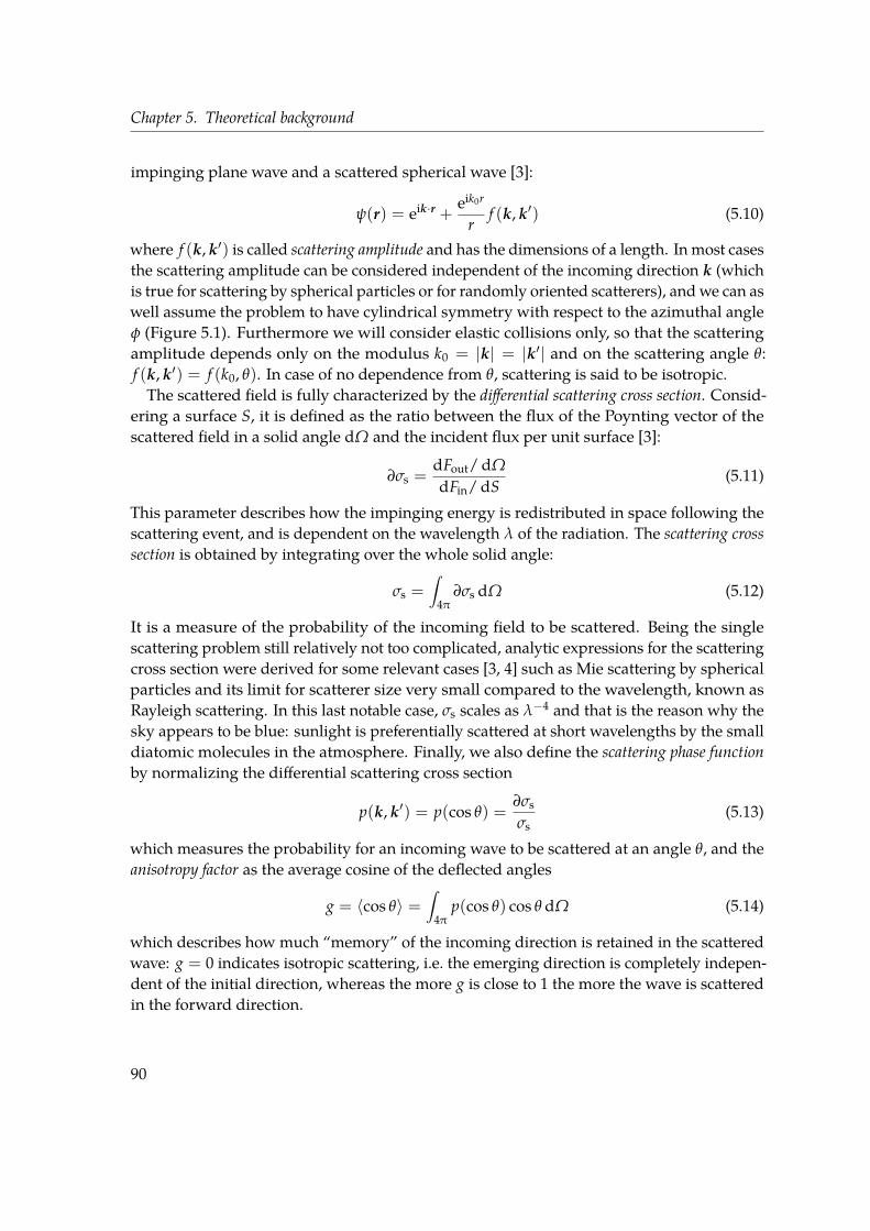
Chapter 5. Theoretical background
impinging plane wave and a scattered spherical wave [3]:
ψ(r) = eik·r +eik0r
rf (k, k′) (5.10)
where f (k, k′) is called scattering amplitude and has the dimensions of a length. In most casesthe scattering amplitude can be considered independent of the incoming direction k (whichis true for scattering by spherical particles or for randomly oriented scatterers), andwe can aswell assume the problem to have cylindrical symmetry with respect to the azimuthal angleφ (Figure 5.1). Furthermore we will consider elastic collisions only, so that the scatteringamplitude depends only on the modulus k0 = |k| = |k′| and on the scattering angle θ:f (k, k′) = f (k0, θ). In case of no dependence from θ, scattering is said to be isotropic.The scattered field is fully characterized by the differential scattering cross section. Consid-
ering a surface S, it is defined as the ratio between the flux of the Poynting vector of thescattered field in a solid angle dΩ and the incident flux per unit surface [3]:
∂σs =dFout/ dΩ
dFin/ dS(5.11)
This parameter describes how the impinging energy is redistributed in space following thescattering event, and is dependent on the wavelength λ of the radiation. The scattering crosssection is obtained by integrating over the whole solid angle:
σs =∫
4π∂σs dΩ (5.12)
It is a measure of the probability of the incoming field to be scattered. Being the singlescattering problem still relatively not too complicated, analytic expressions for the scatteringcross section were derived for some relevant cases [3, 4] such as Mie scattering by sphericalparticles and its limit for scatterer size very small compared to the wavelength, known asRayleigh scattering. In this last notable case, σs scales as λ−4 and that is the reason why thesky appears to be blue: sunlight is preferentially scattered at short wavelengths by the smalldiatomic molecules in the atmosphere. Finally, we also define the scattering phase functionby normalizing the differential scattering cross section
p(k, k′) = p(cos θ) =∂σsσs
(5.13)
which measures the probability for an incoming wave to be scattered at an angle θ, and theanisotropy factor as the average cosine of the deflected angles
g = 〈cos θ〉 =∫
4πp(cos θ) cos θ dΩ (5.14)
which describes how much “memory” of the incoming direction is retained in the scatteredwave: g = 0 indicates isotropic scattering, i.e. the emerging direction is completely indepen-dent of the initial direction, whereas the more g is close to 1 the more the wave is scatteredin the forward direction.
90

5.3. Multiple scattering
(a) (b) (c)
Figure 5.2.: Light propagating in different scattering regimes, modified from [5]. (a) When thereis no scattering, light passes undisturbed through the sample (ballistic light). (b) Single scatteringregime from sparse scatterers. (c) Multiple scattering regime from dense scatterers.
5.3. Multiple scattering
As mentioned in the previous section, the single scattering regime is relatively easy tostudy and it is successfully applied to describe relevant phenomena such as diffusion oflight by the atmosphere. In this regime, a wave propagating through a scattering mediumwill have undergone a number of scattering events close to one. In other cases, involv-ing bigger and denser scatterers such as water droplets in clouds, a multiple-scatteringregime sets in. This is the case of what happens with many objects encountered duringeveryday life, such as milk, foams, paper, snow, fog and clouds. All of these materialsshare similar looks in that they are appear to be white and opaque. Indeed, in a multiple-scattering regime, the dependence of the scattering cross section on the radiation wavelengthis not enough to determine a spectral selection of the scattered waves, so that light in abroad frequency range is back-diffracted in random directions causing the white opaqueaspect.The different scattering regimes so far outlined are illustrated in Figure 5.2. As shown
in panel c), a turbid medium can be thought of as an ensemble of point-like centres placedrandomly inside the material. In such configuration, modelling the multiple-scatteringproblem in the framework of the wave theory of light is not trivial. Some techniques existin which the total scattered field is first written as the superposition of the partial fieldsscattered by the individual particles and then the so-called Foldy-Lax equations are iteratedto finally derive an expansion for the scattered field [6]. However, these methods require theposition of each scattering centre to be known in advance (what is called quenched disorder,where scatterers are found at determined positions) and many iterations on the scatteredfields are needed. As the number of scatterers increases, these techniques become soonunsuitable for an efficient description.
91

Chapter 5. Theoretical background
As anticipated, in order to make the multiple-scattering problem more easily manageable,it is best to drop the deterministic description using fixed scatterers in favour of a statisticalapproach. In a homogeneously disordered sample, scatterers are randomly distributed witha constant density ρs so that we can identify the average distance ls between two consecutivescattering events as a characteristic property of the material, called scattering mean free path.We also define the scattering rate as
µs = σsρs =1ls
(5.15)
which measures the probability per unit length of a propagating wave of being scattered inanother direction. In order to fully characterize the turbid material, in addition to scatteringwe need to consider absorption as well, since part of the incident energy may be absorbed byatoms or molecules in the medium. Therefore, in full analogy we also define the absorptionrate and the absorption mean free path
µa = σaρa =1la
(5.16)
where ρa is the density of absorbers. When a wave of intensity I travels for a distance Linside an absorbing medium, its intensity decreases according to the Lambert-Beer law:
I = I0 exp(−µaL) (5.17)
Absorption is not the only process causing a decrease in the observed intensity: the energyredistributed in other directions because of scattering appears to be “lost” as well. Wheninvestigating microscopic optical properties such as ls, absorption is often a hindrance sinceit is not easy to decouple its effect from that of scattering. For what is said above we alsodefine the total extinction rate µe as
µe = µs + µa (5.18)
and the single-scattering albedoa =
µsµe
(5.19)
With the parameters introduced above we are able to describe the average scatteringproperties of a turbid material. Of course these quantities are meaningful as long as the farfield approximation that we used since the beginning is holding, that is to say in the limitwhere the scattering mean free path is longer than the radiation wavelength, so that for eachscattering event the theory outlined for the single scattering regime can still be used. Withthese basic concepts laid out, in the following section we shall see how light transport inturbid media can be modelled in the framework of Radiative Transport Theory (RTT).
92

5.4. The Radiative Transport Equation
5.4. The Radiative Transport Equation
The Radiative Transport Theory dates back to the end of 19th century, when it was firstderived to model light transport in foggy atmospheres [7]. It later found many applicationsin different areas of science and engineering, such as in astrophysics where it is used todescribe light propagation through the interstellar medium and in stellar atmospheres. Morerecently, light transport in biological tissues has become the object of study of the growingfield of biomedical optics and diagnostics [8].
In the following we are going to write the equation which lies at the core of the RadiativeTransport Theory, known as Radiative Transport Equation (RTE). In terms of its formulation,the RTE is a very simple equation, in that it is simply an energy balance equation statingenergy conservation inside a small test volume. Here we will describe the equation throughthe heuristic and intuitive point of view which was used when the equation was firstformulated. Recently though it was shown that the RTE can be rigorously derived fromMaxwell’s equations [9], thus recovering the initially missing formal link with wave theory.We start by assuming scattering events as point-like collisions both in space and time,
and by requiring that there be no correlations in the position of scattering centres so thatinterference effects between scattered waves can be ignored. Considering a small volume V,the RTE is simply written by balancing the flow of energy entering and leaving that volumealong a direction s [8, 10, 11]:
1v
∂I(r, t, s)∂t
= −s · ∇I(r, t, s)− µe I(r, t, s) +µe4π
∫
4πp(s, s′)I(r, t, s′)dΩ′ + Q(r, t, s) (5.20)
where I(r, t, s) is the radiance or specific intensity measured in Wm−2 sr−1. The variation intime of the radiance on the left-hand side is balanced on the right-hand side by four termswhich we can identify as follows:
1. the change in radiance due to energy entering and leaving the volume through itsboundaries;
2. the losses due to absorption and scattering;
3. the gain due to scattering into the direction s from another direction s′;
4. radiance gain due to possible sources inside the volume.
It is worth noting that in the RTE the wave nature of light is completely lost; its link withwave propagation is retained only in the scattering coefficient and scattering phase function.Electromagnetic energy is indeed considered to be carried by rays of light in the geometricaloptics sense. As we will soon see, this is a first step towards a description of light scatteringand propagation in terms of a random walk of fictitious energy-carrying particles.Despite its simple formulation, the RTE can’t be easily solved analytically. Before seeing
how to tackle the problem of solving the RTE, we can observe two properties of its solutions
93

Chapter 5. Theoretical background
[11]. First, considering a source term of unitary strength
Q(r, t, s) = δ(r)δ(t)δ(s) (5.21)
where δ is the Dirac delta function, if I(r, t, s) is a solution of the RTE then
I(r, t, s) =(
µeµe
)3
I(r, t, s) (5.22)
withr = r
µeµe
t = tµeµe
(5.23)
is a solution for amediumhaving an extinction coefficient µe and the same scattering functionand albedo. This is also known as similarity principle and it allows to scale the results foranother geometry, provided the same albedo and scattering function are kept the same.Second, if I(r, t, s′)|µa=0 is the solution for a nonabsorbing medium, then
I(r, t, s′) = exp(−µavt)I(r, t, s′)|µa=0 (5.24)
is a still a solution to the same equation when the absorption coefficient µa is independentof r.
5.5. The Diffusion Approximation
Given its complexity, the RTE cannot be solved directly. Several approximations have tobe made in order to attempt an analytical approach. One method consists in writing theradiance as an expansion of spherical harmonic functions truncated after N terms, whichis known as the PN-approximation. In particular, we will show that applying this methodwith N = 1 leads to the so-called Diffusion Approximation (DA).
Let’s consider an isotropic source emitting a pulse of energy E0 [11]:
Q(r, t, s) = Q0(r, t) =E0
4πδ(r− r′)δ(t) (5.25)
When scattering is stronger than absorption, we can assume the radiance to be almostisotropic plus a small directional flux:
I(r, t, s) =1
4πUd(r, t) +
34π
Fd(r, t) · s (5.26)
whereUd(r, t) =
∫
4πI(r, t, s)dω (5.27)
is the average diffuse intensity and
Fd(r, t) =∫
4πI(r, t, s)s dω = Fd(r, t)sf (5.28)
94

5.5. The Diffusion Approximation
is the diffuse flux vector. By inserting equations (5.25) and (5.26) into the RTE (5.20) andintegrating — over the whole solid angle — the RTE and the RTE multiplied by s, we obtainthe following coupled equations:
(1v
∂
∂t+ µ′s
)Fd(r, t) +
13∇Ud(r, t) = 0 (5.29)
1v
∂
∂tUd(r, t) +∇Fd(r, t) = Q0(r, t) (5.30)
whereµ′s = (1− g)µs (5.31)
is known as the reduced scattering coefficient. As usual, we also assume that the scatteringphase function depends only on the scattering angle between s and s′. Finally, we assumethe variation in time of the flux vector to be negligible over a length scale of the order of thetransport mean free path
lt =1µ′s
=1
(1− g)µs(5.32)
In formulas: ∣∣∣∣1
vµ′s
∂Fd(r, t)∂t
∣∣∣∣ |Fd(r, t)| (5.33)
With these assumptions, equation (5.29) becomes
Fd(r, t) = −1v
D∇Ud(r, t) (5.34)
known as Fick’s equation of diffusion, where D is the diffusion coefficient
D =v
3µ′s=
13(1− g)µs
=13
vlt (5.35)
measured in m2 s−1. By inserting Fick’s equation back into equation (5.30) we finally obtainthe Diffusion Equation (DE) [11, 12]:
1v
(∂
∂t− D∇2
)Ud(r, t) = Q0(r, t) (5.36)
For a source emitting an isotropic pulse as in equation (5.25), a general solution for the DEin an infinitely extended nonabsorbing medium is given by:
Ud(r, t) = E0v
(4πDt)3/2 exp(−|r− r′|2
4Dt
)(5.37)
which according to equation (5.24) can be easily extended for the case of an absorbingmedium by simple multiplication by exp(−µavt). The diffused intensity thus exhibits aGaussian profile in space which broadens in time.
95

Chapter 5. Theoretical background
5.6. Diffusion in bounded media
In the previous section a solution of the DE was derived in the case of an infinitely extendedmedium. For most practical cases though, a more interesting geometry is that of a scatteringmedium with finite size along at least one dimension, that is to say a layer or a slab. Theslab geometry is indeed used in many applications as a simple representation for biologicaltissues, a compressed breast or a layer of paint, just to make a few examples. It is thereforeof primary interest to derive analytical expressions for this relevant case.
Let’s consider a slab made of a scattering medium, having infinite dimensions along the xand y directions and a finite thickness L along z. Since the diffusing medium is bounded bya surface Σ, we have to impose some boundary condition for the diffuse specific intensityI(r, t, s) on that interface. Several different boundary conditions have been used to treatthe problem of a finite medium [13]. In the simplest case, when there is no refractive indexmismatch across the interface, the boundary is perfectly transmitting (i.e. there are no Fresnelreflections), so that all the light crossing the interface will leave the sample. In other wordswe assume perfectly absorbing boundary conditions by asking that, for r on Σ and s directedinward, there should be no diffuse light entering the medium (Zero Boundary Condition) [11,13]:
I(r, t, s) = 0 (5.38)
However, because of the earlier assumption that the intensity be almost isotropic (5.26), suchcondition cannot be satisfied exactly. Therefore we can only look for approximate boundaryconditions. The simplest approximation states that on the external surface the total diffuseflux directed inward must be zero [11, 12]:
∫
s·n>0I(r, t, s)(s · n)dΩ = 0 (5.39)
for r on Σ and where n is the inward normal to the interface surface Σ. We now consider theflux at the two boundaries in z = 0 and z = L. In case of no reflections, imposing a null fluxincoming from outside the slab leads to the two following boundary conditions [14, 15]:
U − 2lt3
∂U∂z
= 0 at z = 0
U +2lt3
∂U∂z
= 0 at z = L(5.40)
If we assume that ∂U/∂z is constant inside the sample near the boundaries and pretendthat we can extend the solutions outside the sample by linear extrapolation, then the twoconditions above are equivalent to require that U be zero at the fictitious coordinates z = −zeand z = L + ze where ze is called extrapolated length:
ze =2Dv
=23
lt (5.41)
96

5.6. Diffusion in bounded media
assuming the slab is placed at z = 0. This is known as Extrapolated Boundary Condition (EBC)and basically relates the sample thickness L with a fictitious thickness Leff = L + 2ze thatwould make the specific intensity vanish assuming we linearly extrapolate its derivativenear the boundaries. In case of refractive index mismatch between the sample and theenvironment, the total diffuse flux at the boundary directed inward into the medium mustequate the reflected fraction of the flux directed outward so that equation (5.39) becomes:
∫
s·n>0I(r, t, s)(s · n)dΩ =
∫
s·n<0R(s)I(r, t, s)|s · n|dΩ (5.42)
again for r on Σ and where R(s) is the Fresnel reflection coefficient for unpolarized light:
R(s) =12
[(n cos θi − cos θtn cos θi + cos θt
)2
+
(cos θi − n cos θtcos θi + n cos θt
)2]
(5.43)
In the equation above n = nin/nout is the refractive index contrast between the sample andthe environment, whereas θi (cos θi = −s · q) and θt = arcsin(n sin θi) are the incident andrefracted angle respectively. From equations (5.42) and (5.26) we have
Ud(r, t) +A2π
Fd(r, t) · n = 0 (5.44)
where the coefficient
A =1 + 3
∫ π/20 R(θi) cos2 θi sin θi dθi
1− 2∫ π/2
0 R(θi) cos θi sin θi dθi(5.45)
can be found in the literature written as an expansion of n [11]. In this case equation (5.41)becomes:
ze =2AD
v=
23
Alt (5.46)
By intuition we can state that a reasonable assessment of boundary conditions is importantin order to obtain accurate results, especially for optically thin samples (L lt) whereapproximations such as (5.39) are more easily disobeyed. The presence of a refractiveindex mismatch at the interface between the diffusing medium and the environment cansignificantly alter the magnitude of the specific intensity inside the medium as well asthe determination of the microscopic transport parameters such as lt. For example, for arefractive index contrast n ≈ 1.4 (a typical value for biological tissues) from equation (5.43)follows that the boundaries reflect more than 50% of light back into the sample, with theresult that from the point of view of diffusion the slab appears to be thicker than it reallyis. Additionally, a striking effect of the presence of reflections at the boundaries is that thefraction of transmitted light is heavily altered by the presence of ze, even for optically thicksamples (L lt) [14]:
T =lt + zeL + 2ze
(5.47)
97

Chapter 5. Theoretical background
k
ρ
z
0 L
−ze L + ze
lt2(ze + lt)
positive sources
negative sources
nout nin
Figure 5.3.: A pencil beam impinging on an infinite slab can be modelled as an isotropic sourcelocated at z = lt inside the sample. Extrapolated Boundary Conditions are met by considering aninfinite series of positive and negative sources [11].
We now turn to finding a solution for the time-dependent DE in the slab geometry asshown in Figure 5.3. Herewe consider a pencil beam of pulsed light impinging normally to theslab entrance surface placed at z = 0, that is we take a thin and collimated beam describedin the time domain by a Dirac delta function. This is a good approximation for an ultrashortlaser pulse, with geometrical dimensions much smaller than the sample size, which istypically used in real case experiments to probe light transport and diffusion in scatteringmedia. However, the DE as derived in section 5.5 was obtained with the assumption of anisotropic source (5.25) and cannot be used for an impinging beam as in this case.
Several methods can be used to model a pencil beam within our derivation of the DE. Forexample, the monodirectional source can be modelled [12, 16] as a continuous distributionof point-like sources located along the slab thickness, having an intensity proportional toµs exp(−zµt) (the probability for ballistic light to penetrate the sample at a depth z) andan angular distribution given by the scattering function. A simpler further approximationcan be made, is the slab is much thicker than the scattering mean free path, by replacingthe pencil beam with a single isotropic source located at z = lt inside the sample [17]. Thischoice can be explained by considering that, upon entering the slab, the incoming light willkeep on propagating along z before being isotropically scattered for the first time, an eventwhich will happen on average at a depth z = lt. The error introduced by this approximationis of course more relevant for thin slabs.Following the latter approach, we here consider a pulse of energy E0 emitted by an
isotropic point source located at z = lt:
Q(r, t) =E0
4πδ(x)δ(y)δ(z− lt)δ(t) (5.48)
We assume Extrapolated Boundary Conditions, i.e. an average diffuse intensity vanishing
98
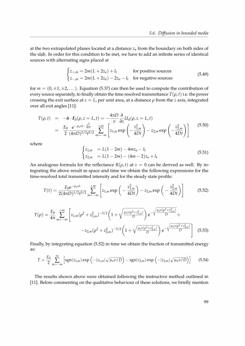
5.6. Diffusion in bounded media
at the two extrapolated planes located at a distance ze from the boundary on both sides ofthe slab. In order for this condition to be met, we have to add an infinite series of identicalsources with alternating signs placed at
z+,m = 2m(L + 2ze) + lt for positive sourcesz−,m = 2m(L + 2ze)− 2ze − lt for negative sources
(5.49)
for m = (0,±1,±2, . . . ). Equation (5.37) can then be used to compute the contribution ofevery source separately, to finally obtain the time resolved transmittance T(ρ, t) i.e. the powercrossing the exit surface at z = L, per unit area, at a distance ρ from the z axis, integratedover all exit angles [11]:
T(ρ, t) = −n · Fd(ρ, z = L, t) = −4πDv
∂
∂zUd(ρ, z = L, t)
=E0
2e−µavt− ρ2
4Dt
(4πD)3/2t5/2
+∞
∑m=−∞
[z1,m exp
(−
z21,m
4Dt
)− z2,m exp
(− z2
2,m
4Dt
)] (5.50)
where z1,m = L(1− 2m)− 4mze − ltz2,m = L(1− 2m)− (4m− 2)ze + lt
(5.51)
An analogous formula for the reflectance R(ρ, t) at z = 0 can be derived as well. By in-tegrating the above result in space and time we obtain the following expressions for thetime-resolved total transmitted intensity and for the steady state profile:
T(t) =E0e−µavt
2(4πD)1/2t3/2
+∞
∑m=−∞
[z1,m exp
(−
z21,m
4Dt
)− z2,m exp
(− z2
2,m
4Dt
)](5.52)
T(ρ) =E0
4π
+∞
∑m=−∞
[z1,m(ρ
2 + z21,m)
−3/2(
1 +
√µav(ρ2+z2
1,m)
D
)e−√
µav(ρ2+z21,m)
D +
−z2,m(ρ2 + z2
2,m)−3/2
(1 +
√µav(ρ2+z2
2,m)
D
)e−√
µav(ρ2+z22,m)
D
](5.53)
Finally, by integrating equation (5.52) in time we obtain the fraction of transmitted energyas:
T =E0
2
∞
∑m=−∞
[sgn(z1,m) exp
(−|z1,m|
õav/D
)− sgn(z2,m) exp
(−|z2,m|
õav/D
)](5.54)
The results shown above were obtained following the instructive method outlined in[11]. Before commenting on the qualitative behaviour of these solutions, we briefly mention
99

Chapter 5. Theoretical background
another derivation method based on eigenmode expansion, leading to formulas highlightinginteresting properties. We consider the diffusion equation in the presence of absorption:
1v
(∂
∂t− D∇2 + vµa
)Ud(r, t) = Q(r, t) (5.55)
Given the cylindrical symmetry in the slab geometry, it is best to separate the spatial coor-dinate r in a transverse component r⊥ and a longitudinal one z. Considering a point-likesource in z = lt, we take the Fourier transform in the spatial transverse component and theLaplace transform in time (with F [U(r⊥)] = U(k⊥) and L [U(t)] = U(s)). The DE thenbecomes [18, 19]:
Dv
(∂2
∂z2 − k2⊥ +
sD
+vµaD
)Ud(z, k⊥, s) = −U0(k⊥, s)δ(z− lt) (5.56)
Using Extrapolated Boundary Conditions a solution of the DE is written as:
Ud(z, κ) =vU0
Dκ
cosh(κ(lt − L + z− ze)) cosh(kze)sinh(L + 2ze)
(5.57)
whereκ2 = k2
⊥ +sD
+1L2a
(5.58)
andL2a =
Dvµa
=13
lsla (5.59)
is the squared average length at which light penetrates the sample before being absorbed.Transmission T and reflection R are defined as the flux computed in z = 0 and z = L
T = F(z = L) (5.60)R = −F(z = 0) (5.61)
and are easily found as functions of κ or s by replacing equation (5.56) in Fick’s equation (5.34).Of course the obtained quantities need to be inversely transformed to have them expressed asfunctions of space and time. For the relevant case of no absorption and considering a pulsedsource (so that its Laplace transform in time is unity) Q(r, t) = E0(r⊥)δ(z− lt)δ(t)/4π, thesolution can be expanded as [20]:
Ud(z, t) =2E0v
L + 2ze
∞
∑n=1
sin(
nπ(l + ze)L + 2ze
)sin(
nπ(z + ze)L + 2ze
)exp
(− n2π2Dt(L + 2ze)2
)(5.62)
Inserting the above equation into Fick’s equation (5.34) yields
F(z, t) = − 2E0Dπ
(L + 2ze)2
∞
∑n=1
n sin(
nπ(l + ze)L + 2ze
)cos
(nπ(z + ze)
L + 2ze
)exp
(− n2π2Dt(L + 2ze)2
)
(5.63)
100
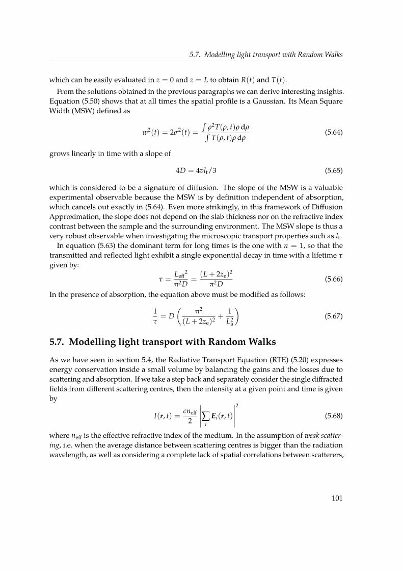
5.7. Modelling light transport with Random Walks
which can be easily evaluated in z = 0 and z = L to obtain R(t) and T(t).From the solutions obtained in the previous paragraphs we can derive interesting insights.
Equation (5.50) shows that at all times the spatial profile is a Gaussian. Its Mean SquareWidth (MSW) defined as
w2(t) = 2σ2(t) =∫
ρ2T(ρ, t)ρ dρ∫T(ρ, t)ρ dρ
(5.64)
grows linearly in time with a slope of
4D = 4vlt/3 (5.65)
which is considered to be a signature of diffusion. The slope of the MSW is a valuableexperimental observable because the MSW is by definition independent of absorption,which cancels out exactly in (5.64). Even more strikingly, in this framework of DiffusionApproximation, the slope does not depend on the slab thickness nor on the refractive indexcontrast between the sample and the surrounding environment. The MSW slope is thus avery robust observable when investigating the microscopic transport properties such as lt.
In equation (5.63) the dominant term for long times is the one with n = 1, so that thetransmitted and reflected light exhibit a single exponential decay in time with a lifetime τ
given by:
τ =Leff
2
π2D=
(L + 2ze)2
π2D(5.66)
In the presence of absorption, the equation above must be modified as follows:
1τ= D
(π2
(L + 2ze)2 +1L2a
)(5.67)
5.7. Modelling light transport with RandomWalks
As we have seen in section 5.4, the Radiative Transport Equation (RTE) (5.20) expressesenergy conservation inside a small volume by balancing the gains and the losses due toscattering and absorption. If we take a step back and separately consider the single diffractedfields from different scattering centres, then the intensity at a given point and time is givenby
I(r, t) =cneff
2
∣∣∣∣∣∑iEi(r, t)
∣∣∣∣∣
2
(5.68)
where neff is the effective refractive index of the medium. In the assumption of weak scatter-ing, i.e. when the average distance between scattering centres is bigger than the radiationwavelength, as well as considering a complete lack of spatial correlations between scatterers,
101

Chapter 5. Theoretical background
ls, g 6= 0
lt, g = 0
Figure 5.4.: A random walk performed by a particle being scattered inside a turbid medium. Accord-ing to the similarity relation, an anisotropic random walk (g 6= 0) with a scattering mean free pathof ls can always be mapped to a completely isotropic one (g = 0) but having a scattering mean freepath equal to lt.
then the interference terms average out to zero so that the total intensity is simply given bythe sum of the intensities of the scattered waves:
I(r, t) = ∑i
Ii(r, t) (5.69)
Of course, the wave nature of light cannot be neglected if the scattering is so important thatconsecutive scattering events happen within a single oscillation of the radiation, a regimewhich can lead to Anderson Localization of light [21].
Experimentally, in a typical setting where a light beam impinges on a turbid medium andthe transmitted light is collected, the interference terms in the summation (5.68) will giverise to a random speckle pattern originating from constructive and destructive interferencewhich depends on the exact configuration of scatterers being probed. The speckle pattern isaveraged out by probing different disorder configurations, i.e. by considering a differententrance point in the sample, to obtain an incoherent transmission profile.From the point of view of modelling instead, equation (5.69) allows us to think of light
transport in terms of a random walk of fictitious energy-carrying particles, which opensnew possibilities to find numerical solutions of the RTE. In fact, the RTE can be rewrittenso as to describe the transport of these scalar particles. If N(r, s, t) is the density of suchparticles propagating along a direction s, then the specific intensity is written as I(r, s, t) =N(r, s, t)Ev where E is the energy per particle. The RTE then becomes [5]:
1v
∂N∂t
= −s · ∇N − µeN +µe4π
∫
4πp(s, s′)N dΩ + QN (5.70)
where QN(r, t, s) = Q(r, t, s)/Ev is now the number of particles emitted per unit time,volume and solid angle.
From equation (5.70) it is now clear that solving the RTE is just a matter of tracing particlesinside the scattering medium, following them as they randomly walk from scatterer toscatterer. This can be done for example by implementing a Monte Carlo algorithm as willbe shown in chapter 6, which in the limit of an infinite number of particles yields an exact
102
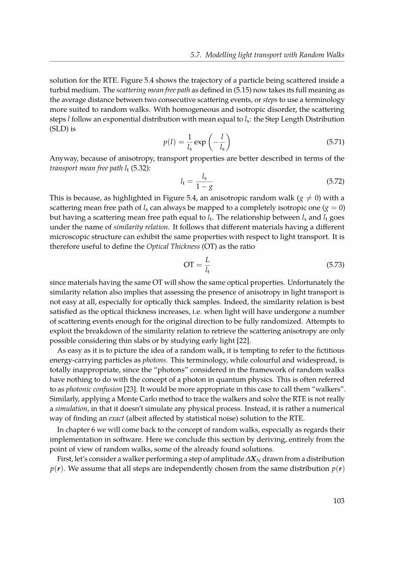
5.7. Modelling light transport with Random Walks
solution for the RTE. Figure 5.4 shows the trajectory of a particle being scattered inside aturbidmedium. The scattering mean free path as defined in (5.15) now takes its full meaning asthe average distance between two consecutive scattering events, or steps to use a terminologymore suited to random walks. With homogeneous and isotropic disorder, the scatteringsteps l follow an exponential distribution with mean equal to ls: the Step Length Distribution(SLD) is
p(l) =1ls
exp(− l
ls
)(5.71)
Anyway, because of anisotropy, transport properties are better described in terms of thetransport mean free path lt (5.32):
lt =ls
1− g(5.72)
This is because, as highlighted in Figure 5.4, an anisotropic random walk (g 6= 0) with ascattering mean free path of ls can always be mapped to a completely isotropic one (g = 0)but having a scattering mean free path equal to lt. The relationship between ls and lt goesunder the name of similarity relation. It follows that different materials having a differentmicroscopic structure can exhibit the same properties with respect to light transport. It istherefore useful to define the Optical Thickness (OT) as the ratio
OT =Llt
(5.73)
since materials having the same OTwill show the same optical properties. Unfortunately thesimilarity relation also implies that assessing the presence of anisotropy in light transport isnot easy at all, especially for optically thick samples. Indeed, the similarity relation is bestsatisfied as the optical thickness increases, i.e. when light will have undergone a numberof scattering events enough for the original direction to be fully randomized. Attempts toexploit the breakdown of the similarity relation to retrieve the scattering anisotropy are onlypossible considering thin slabs or by studying early light [22].
As easy as it is to picture the idea of a random walk, it is tempting to refer to the fictitiousenergy-carrying particles as photons. This terminology, while colourful and widespread, istotally inappropriate, since the “photons” considered in the framework of random walkshave nothing to do with the concept of a photon in quantum physics. This is often referredto as photonic confusion [23]. It would be more appropriate in this case to call them “walkers”.Similarly, applying a Monte Carlo method to trace the walkers and solve the RTE is not reallya simulation, in that it doesn’t simulate any physical process. Instead, it is rather a numericalway of finding an exact (albeit affected by statistical noise) solution to the RTE.
In chapter 6 we will come back to the concept of random walks, especially as regards theirimplementation in software. Here we conclude this section by deriving, entirely from thepoint of view of random walks, some of the already found solutions.
First, let’s consider awalker performing a step of amplitude∆XN drawn from adistributionp(r). We assume that all steps are independently chosen from the same distribution p(r)
103

Chapter 5. Theoretical background
and that they are isotropic, so that p(r) = p(r) and 〈∆XN〉 = 0 (i.e. there are no drifts). LetXN be the position of the walker after N steps
XN =N
∑i
xi =N
∑i
li xi (5.74)
and PN(R) the probability of finding the walker at position R after N steps. For the N + 1-thstep we can write the following recursion [24]:
PN+1(R) =∫
p(r)PN(R− r)ddr (5.75)
where d is the dimensionality of the space in which the random walk takes place. Theequation above holds thanks to the assumption of independence of the steps, which allowsthe probability to step from R− r to R to be factored in the integrand. For N → ∞, thelength scale on which PN(R) varies is much bigger than any typical r, so that we can takethe Taylor expansion:
PN+1(R) =∫
p(r)[
PN(R)− r · ∇PN(R) +12
r · ∇∇PN · r + . . .]
ddr (5.76)
= PN(R)− 0 +12 ∑
i∑
j
⟨rirj⟩ ∂2PN
∂Ri∂Rj+ . . .
= PN(R) +〈r · r〉
2d∇2PN(R) + . . .
If ∆t is the time between two consecutive steps we have t = N∆t and:
PN+1(R)− PN(R)
∆t=
⟨r2⟩
2d∆t∇2PN + . . . (5.77)
In the limit N → ∞ the distribution PN(R) = ρ(R, N∆t) satisfies the Diffusion Equation:
∂ρ
∂t= D∇2ρ (5.78)
with D =⟨r2⟩ /2d∆t. We solve this partial differential equation with the initial condition
ρ(R, 0) = δ(R) (i.e. the walk starts from the origin) by performing a Fourier transform1:
∂ρ
∂t= −Dk2ρ (5.81)
1Here we use the following definitions for Fourier transform and inverse transform:
ρ(k, t) =∫
e−ik·xρ(x, t)ddx (5.79)
ρ(x, t) =1
(2π)d
∫eik·x ρ(k, t)ddk (5.80)
104

5.7. Modelling light transport with Random Walks
This is an ordinary differential equation with solution:
ρ(k, t) = e−Dk2tρ(k, 0) = e−Dk2t (5.82)
which taking the inverse transform becomes:
ρ(R, t) =e−R2/4Dt
(4πDt)d/2 (5.83)
and we have obtained equation (5.37) again. As for the diffusion coefficient in (5.81), using⟨r2⟩ =
⟨l2⟩ and ∆t = 〈l〉 /v it can be written as
D =
⟨r2⟩
2d∆t=
v2d
⟨l2⟩
〈l〉 (5.84)
which for an exponential SLD yields (5.35) D = vlt/3 exactly. Equation (5.84) will play animportant role in our analysis (chapter 8) and it shows how the diffusion coefficient relatesto the first two momenta of the Step Length Distribution.Finally, we derive a powerful expression for the fraction of light transmitted through a
slab by showing that equation (5.47), although following from applying the full DiffusionTheory (DT) formalism or using Green’s function techniques, can also be obtained with asimple reasoning based on random walks [14]. Let’s consider a photon starting a randomwalk at a depth z = lt inside the slab and stopping either at zB = −ze and zR = L + zein case it is reflected or transmitted, respectively. For a photon reaching the centre ofthe slab, the probabilities of being transmitted or reflected must be the same so that wemust have T(L) = T(L′)/2 where L′ + 2ze = (L + 2ze)/2. We can iterate this reasoningby continuing to divide the remainder of the slab in two halves, so that after N timesT(L) = T[(L+ 2ze)/2N− 2ze]/2N . Eventually, when the slab thickness is twice the transportmean free path, a photon at the slab centre will have 50% probability of being reflected ortransmitted, which stops the recursion: T(2lt) = 1
2 . This yields equation (5.47) directly
TD =lt + zeL + 2ze
(5.85)
and it is easy to verify that this formula satisfies both conditions. This is just the diffusecontribution of transmitted light, to which one should add the ballistic contribution ofunscattered light (though it decays exponentially with increasing slab thickness: TB = e−L/ls)in order to obtain the total transmission.
105


Chapter 6.
MCPlusPlus: a Monte Carlo C++ code forradiative transport
I’m personally convinced that computer sciencehas a lot in commonwith physics. Both are abouthow the world works at a rather fundamentallevel. The dierence, of course, is that while inphysics you’re supposed to figure out how theworld is made up, in computer science you createthe world. Within the confines of the computer,you’re the creator. You get to ultimately controleverything that happens. If you’re good enough,you can be God. On a small scale.
(Linus Torvalds)
In this chapter we introduce MCPlusPlus, a Monte Carlo software library for the transport of lightthrough a multilayered system which was developed from scratch entirely in the framework of thisthesis. A short overview of Monte Carlo methods and of the internal structure of MCPlusPlus aregiven, highlighting the improvements of our software over existing Monte Carlo solutions.
6.1. Introducing MCPlusPlus
To perform the simulations presented in this workwe developed a newMonte Carlo softwarelibrary, calledMCPlusPlus, for the transport of light through a multilayered sample. Thissoftware was created from scratch aiming at enriching existing multilayer Monte Carlosoftware such as MCML [25] or CUDAMCML [26] and is made publicly available online [27].Being developed entirely in C++, the program extensively takes advantage of the object-oriented programming paradigm (OOP), which is particularly suited to model a randomwalk problem [28]. Since pieces of code can be encapsulated in reusable objects, OOP offersseveral advantages including scalability, modularity, ease of maintenance and abstraction. Ofequal importance is the fact that OOP naturally lends itself as a tool to describe a high-levelinterface to the software itself. Indeed,MCPlusPlus comes as a shared library rather than anexecutable package. As a notable feature, a Python interface to the library is also provided
107

Chapter 6. MCPlusPlus: a Monte Carlo C++ code for radiative transport
#!/usr/bin/python
from pymcplusplus import *
#define a sample consisting of two layers of different materialssample = Sample ()
#add a layer of material mat and thickness 1000ummat = Material ()mat.n = 1.5mat.g = 0mat.ls = 1000
sample.addLayer(mat ,1000)
#add a layer of material mat2 and thickness 500ummat2 = Material ()mat2.n = 1.3mat.g = 0.5mat.ls = 700
sample.addLayer(mat2,500)
externalMaterial = Material ()externalMaterial.n = 1
sample.setSurroundingEnvironment(externalMaterial)
#define a photon sourcesource = PencilBeamSource ()
#define the main simulation object , simulate 1e10 photons using 8 parallel threads.#note that each thread will use increasing seeds starting from 0sim = Simulation ()sim.setSample(sample)sim.setSource(source)sim.setNPhotons(10000000000)sim.setNThreads(8)sim.setSeed(0)sim.setOutputFileName("example.h5")
#define and add several histograms to the simulation
# 1) a histogram of the exit timeshist = Histogram ()hist.setDataDomain(DATA_TIMES)hist.setPhotonTypeFlags(FLAG_TRANSMITTED)hist.setMax(1000)hist.setBinSize(2)hist.setName("times")hist.setSpatialVarianceEnabled(True)sim.addHistogram(hist)
# 2) a histogram of the exit distances from the centerhist = Histogram ()hist.setDataDomain(DATA_POINTS );hist.setPhotonTypeFlags(FLAG_TRANSMITTED)hist.setMax(1000000)hist.setBinSize(50)hist.setName("points")sim.addHistogram(hist)
# 3) a bivariate histogram of the exit distances as a function of timehist = Histogram ()hist.setDataDomain(DATA_POINTS , DATA_TIMES)hist.setPhotonTypeFlags(FLAG_TRANSMITTED)hist.setMax(100000,1000)hist.setBinSize(500,2)hist.setName("points_vs_times")sim.addHistogram(hist)
# run the simulationsim.run()
Figure 6.1.: Example of simulation with MCPlusPlus using the Python scripting interface. The sam-ples consists of two layers of different materials and a pencil beam is used for the source. 1010 photonsare simulated on 8 parallel threads. Several histograms to be saved to the output file are configured.
108
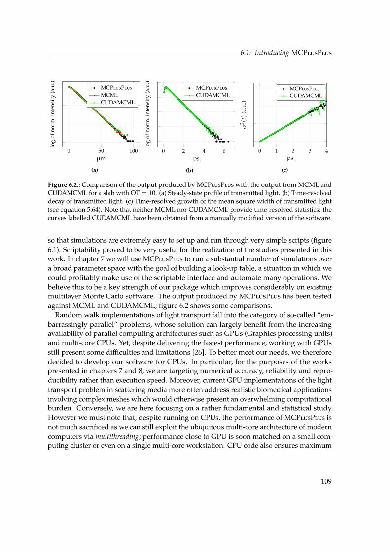
6.1. Introducing MCPlusPlus
0 50 100µm
log
ofno
rm.i
nten
sity
(a.u
.)
MCPlusPlusMCMLCUDAMCML
(a)
0 2 4 6ps
log
ofno
rm.i
nten
sity
(a.u
.)
MCPlusPlusCUDAMCML
(b)
0 1 2 3 4ps
w2 (
t)(a
.u.)
MCPlusPlusCUDAMCML
(c)
Figure 6.2.: Comparison of the output produced by MCPlusPlus with the output from MCML andCUDAMCML for a slab with OT = 10. (a) Steady-state profile of transmitted light. (b) Time-resolveddecay of transmitted light. (c) Time-resolved growth of the mean square width of transmitted light(see equation 5.64). Note that neither MCML nor CUDAMCML provide time-resolved statistics: thecurves labelled CUDAMCML have been obtained from a manually modified version of the software.
so that simulations are extremely easy to set up and run through very simple scripts (figure6.1). Scriptability proved to be very useful for the realization of the studies presented in thiswork. In chapter 7 we will use MCPlusPlus to run a substantial number of simulations overa broad parameter space with the goal of building a look-up table, a situation in which wecould profitably make use of the scriptable interface and automate many operations. Webelieve this to be a key strength of our package which improves considerably on existingmultilayer Monte Carlo software. The output produced by MCPlusPlus has been testedagainst MCML and CUDAMCML; figure 6.2 shows some comparisons.Random walk implementations of light transport fall into the category of so-called “em-
barrassingly parallel” problems, whose solution can largely benefit from the increasingavailability of parallel computing architectures such as GPUs (Graphics processing units)and multi-core CPUs. Yet, despite delivering the fastest performance, working with GPUsstill present some difficulties and limitations [26]. To better meet our needs, we thereforedecided to develop our software for CPUs. In particular, for the purposes of the workspresented in chapters 7 and 8, we are targeting numerical accuracy, reliability and repro-ducibility rather than execution speed. Moreover, current GPU implementations of the lighttransport problem in scattering media more often address realistic biomedical applicationsinvolving complex meshes which would otherwise present an overwhelming computationalburden. Conversely, we are here focusing on a rather fundamental and statistical study.However we must note that, despite running on CPUs, the performance of MCPlusPlus isnot much sacrificed as we can still exploit the ubiquitous multi-core architecture of moderncomputers via multithreading; performance close to GPU is soon matched on a small com-puting cluster or even on a single multi-core workstation. CPU code also ensures maximum
109

Chapter 6. MCPlusPlus: a Monte Carlo C++ code for radiative transport
hardware compatibility, while GPU-based implementations are hardware or even vendorspecific. Additionally, developing software for a pure CPU architecture has generally lesscomplications than writing GPU-compatible code; plenty of software libraries and high-quality Pseudo-Random Number Generators (PRNGs) are widely available for the CPU,providing us with the flexibility and freedom that we needed for the purpose of this work.
Finally, the extent of the simulations that wewill describe in the next chapter and especiallyin chapter 8 is particularly significant (up to 1014 photons), a fact which alone poses severalchallenges. Indeed, simulating such a large number of photons requires the use of 64-bitPRNGs in place of the more common 32-bit implementations, which would introduce astatistically significant truncation in the sampled distributions as better explained in thefollowing section. Accordingly, the correct representation of the random variates requiresthe use of long double floating point notation. Both these requirements are straightforwardon a CPU architecture, as opposed to GPUs, supporting our preference for the former.
6.2. The Monte Carlo method
Monte Carlo (MC) methods encompass a broad class of computational algorithms aimed atsolving a deterministic problem, whose analytic solution is often lacking or impractical, byrepeatedly sampling a probabilistic description of an analogue model. As the number ofobservations goes to infinity the estimate approaches the true value, therefore the MonteCarlo method provides an exact solution to the original problem. However, being basedon random sampling, that solution is affected by statistical noise, which decreases withan increasing number of trials. A simple typical example of a Monte Carlo technique isthe determination of the area of a lake having a generic shape. The problem is solved byenclosing the lake within a square, the area of which is easily calculated, and then throwinga number of point-like stones uniformly over the square area, counting how many of themfall inside or outside the lake. The ratio of the number of stones that fell into the lake andthe number of stones that fell outside the lake is then an estimate of the ratios of the twoareas. As the number of launched stones goes to infinity, the estimate becomes exact.
At the heart of a Monte Carlo method is the ability to sample random variables with well-defined probability distributions. Therefore, a good source of random numbers is neededfor this purpose. Truly random numbers can only be generated by observing an inherentlyrandom physical process, such as radioactive decay or some other quantum process (see sec-tion 1.3.3). However, while truly random numbers are required for applications concerningcryptography, their use in many other applications — such as Monte Carlo methods — is notonly impractical but also unneeded. Within a computer, pseudorandom are more efficientlyproduced through Pseudo-Random Number Generators (PRNGs), i.e. algorithms whichgenerate a deterministic sequence of numbers which approximate the properties of a trulyrandom sequence. In practice, they are periodic sequences with an extremely high period.MCPlusPlusmakes use of the PRNGs implemented in the Boost C++ libraries. In particular
110

6.2. The Monte Carlo method
we chose the broadly used Mersenne Twister algorithm which is fast while providing goodperformances1.
Let us consider a random variable χ, with a Probability Density Function (PDF) p(χ)normalized such that ∫ b
ap(χ)dχ = 1 (6.1)
Random numbers with an arbitrary PDF are usually generated starting from another randomvariable ξ uniformly distributed in the interval (0, 1), provided by the computer. TheCumulative Distribution Function (CDF) F(ξ) of this variable is thus
Cξ(ξ) =
0 if ξ ≤ 0
ξ if 0 < ξ ≤ 1
1 if ξ > 0
(6.2)
To sample the generic p(χ), we assume the existence of a nondecreasing function f (ξ) = χ
which provides a one-to-one mapping between ξ ∈ (0, 1) and χ ∈ (a, b) [29]. Therefore thefollowing equalities hold between the probabilities:
P f (0) < χ ≤ f (ξ1) = P0 < ξ ≤ ξ1 → Pa < χ ≤ χ1 = P0 < ξ ≤ ξ1 (6.3)
The equalities above can be changed to an equation of CDFs:
Cχ(χ1) = Cξ(ξ1) (6.4)
Using the definition of CDF and equation (6.2), the last expression becomes:∫ χ1
ap(χ)dχ = ξ1 for ξ ∈ (0, 1) (6.5)
Finally, solving for χ1 yields the sought function f (ξ1). A prominent example is the case of arandom variable following an exponential distribution, such as the Step Length Distribution(SLD) that we will use for the random walk process. In this case
p(l) =1ls
exp(− l
ls
)(6.6)
Equation (6.5) yields an expression for a sample variate l1 based on the random variate ξ1:
ξ1 =∫ l1
0p(l)dl = 1− el1/ls (6.7)
1The standard Mersenne Twister algorithm has a period of 219937−1 and good uniform distribution in up to623 dimensions for the 32-bit version (up to 311 dimensions for the 64-bit version). It also passes severaltests for statistical randomness.
111
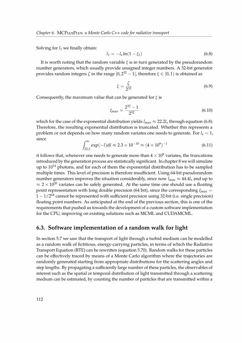
Chapter 6. MCPlusPlus: a Monte Carlo C++ code for radiative transport
Solving for l1 we finally obtain:l1 = −ls ln(1− ξ1) (6.8)
It is worth noting that the random variable ξ is in turn generated by the pseudorandomnumber generators, which usually provide unsigned integer numbers. A 32-bit generatorprovides random integers ζ in the range [0, 232 − 1], therefore ξ ∈ [0, 1) is obtained as
ξ =ζ
232 (6.9)
Consequently, the maximum value that can be generated for ξ is
ξmax =232 − 1
232 (6.10)
which for the case of the exponential distribution yields lmax ≈ 22.2ls through equation (6.8).Therefore, the resulting exponential distribution is truncated. Whether this represents aproblem or not depends on how many random variates one needs to generate. For ls = 1,since ∫ ∞
22.2exp(−l)dl ≈ 2.3× 10⁻¹⁰ ≈ (4× 10⁹)−1 (6.11)
it follows that, whenever one needs to generate more than 4× 10⁹ variates, the truncationsintroduced by the generation process are statistically significant. In chapter 8wewill simulateup to 1014 photons, and for each of them the exponential distribution has to be sampledmultiple times. This level of precision is therefore insufficient. Using 64-bit pseudorandomnumber generators improves the situation considerably, since now lmax ≈ 44.4ls and up to≈ 2× 10²⁰ variates can be safely generated. At the same time one should use a floatingpoint representation with long double precision (64 bit), since the corresponding ξmax =
1− 1/264 cannot be represented with sufficient precision using 32-bit (i.e. single precision)floating point numbers. As anticipated at the end of the previous section, this is one of therequirements that pushed us towards the development of a custom software implementationfor the CPU, improving on existing solutions such as MCML and CUDAMCML.
6.3. Software implementation of a random walk for light
In section 5.7 we saw that the transport of light through a turbid medium can be modelledas a random walk of fictitious, energy-carrying particles, in terms of which the RadiativeTransport Equation (RTE) can be rewritten (equation 5.70). Randomwalks for these particlescan be effectively traced by means of a Monte Carlo algorithm where the trajectories arerandomly generated starting from appropriate distributions for the scattering angles andstep lengths. By propagating a sufficiently large number of these particles, the observables ofinterest such as the spatial or temporal distribution of light transmitted through a scatteringmedium can be estimated, by counting the number of particles that are transmitted within a
112

6.3. Software implementation of a random walk for light
given bin in space and time. It is worth stressing again that, within the algorithm, no actualsimulation of physical processes takes place. Simply, a large number of random trajectoriesare generated in order to statistically sample the RTE and converge to an exact solution.Similarly, these fictitious particles have nothing to do with photons in the quantum sense.In fact, in this chapter we will refer to them as “walkers” to highlight their relationship witha random walk. For convenience we will nonetheless call them photons in chapters 7 and 8,which is accepted in the commonly used terminology.
In this section we describe some implementation details that are specific to MCPlusPlus.More information can be found in the online documentation [27].
6.3.1. Sample description
With MCPlusPlus, a system of multiple semi-infinite slabs can be simulated. The multilayergeometry is described through the Sample class. Each slab is characterized by a finitethickness, expressed in µm, and by a Material. Properties of a Material are its refractiveindex n, its scattering anisotropy g and its scatteringmean free path ls, again expressed in µm.For a non-scattering material, ls is set to infinity. Layers are stacked along increasing valuesof z in a Cartesian coordinate system, with the first slab being placed at z = 0. Finally, tocomplete the description of the simulated geometry, the Material properties of the (possiblydifferent) surrounding environments must be specified.
6.3.2. Source term
In MCPlusPlus, a simulation starts with the creation of a walker at a given position andwith an initial k vector. In most Monte Carlo implementations of light propagation throughscattering slabs, walkers are created at a fixed position and impinge perpendicularly on theslab surface, i.e. the initial k vector is (0, 0, 1). This is often called a pencil beam source, and itcan be defined as a combination of Dirac delta functions in the form δ(r− r0)δ(k− k0).Thanks to the flexibility given by the object-oriented programming paradigm, the in-
structions related to the creation of a walker are not hard-coded in the main body of thesoftware, but they are rather encapsulated within dedicated classes. In our case (figure 6.3)the Source class defines the interface and the basic properties of a generic source, thereforeit acts as a base class. Specific implementations of different sources are given in its derivedclasses. The PencilBeamSource class, for example, implements the pencil beam source thatwe just described. Contrarily to most Monte Carlo packages which provide a pencil beamsource only, with MCPlusPlus several sources are predefined or a custom source can bespecified by the user. Some of the available sources are the IsotropicPointSource and theGaussianRayBundleSource, the latter providing a ray-optic description of a Gaussian beamwaist [30]. The distribution in time of the generated walker can also be specified. For mostcases, the distribution is a Dirac delta δ(t− t0).
113

Chapter 6. MCPlusPlus: a Monte Carlo C++ code for radiative transport
UniformDistribution
Sech2Distribution
Source
Simulation
GaussianRayBundleSource
GaussianBeamSource
PencilBeamSource
IsotropicPointSourceH5OutputFileH5FileHelper
Histogram
Sample
NormalDistribution
IsotropicPsiGenerator
BaseObject
BaseRandom
CosThetaGenerator
AbstractDistribution
ExponentialDistribution
DeltaDistribution
Figure 6.3.:Hierarchy of the main classes within MCPlusPlus internal structure. The arrows connectderived classes to their base class.
yx
z
Figure 6.4.: An example of a GaussianRayBundleSource, one of the specialized sources providedby MCPlusPlus (not used in this work). This source mimics a laser beam focused by a lens; the zcoordinate of the focus can be chosen by the user. In this example, a sample made of three slabs inshown; walker trajectories (rays) are coloured differently within each slab. Here the Gaussian beamis focused on the boundary with the last medium.
114

6.3. Software implementation of a random walk for light
Whatever the choice of the source class, its function is to create a walker in its initial state.It therefore initializes the fields of the Walker class, which is simply a container structurefor storing the position and direction of the walker at each simulation step, according tothe particular distributions for that source. For example, with a PencilBeamSource walkersare always created at the same initial coordinate r0 and with k0 = (0, 0, 1), whereas fora GaussianRayBundleSource the initial distributions of positions and directions is morecomplicated (figure 6.4). Within the Walker class, the current Cartesian coordinates x, y andz of the walker are stored, together with the unit vector k described in terms of its directionalcosines (µx, µy, µz):
µx = k · x µy = k · y µz = k · z (6.12)
where x, y and z are the versors of the Cartesian axes.
6.3.3. Walker propagation
The core of the random walk process is implemented within the Simulation class. This iswhere all the classes defined above converge. Indeed, the task of this class is to propagatethe Walkers produced by the Source through the geometry provided by the Sample class.At each simulation steps, the position and direction of a Walker are updated.
Let us consider the generic n-th step of the random walk process. Suppose that a givenwalker just reached a position r while travelling in a direction k. The software has to propa-gate the walker to a new position r′ and a new direction k′. In other words, each simulationstep represents a scattering event. As we have already mentioned, we are only dealingwith homogeneous media with annealed disorder: in place of simulating the propagationthrough a structure of scattering centres at fixed positions in space (quenched or deterministicdisorder), we are instead building the random walk starting from the statistical distributionof the step lengths and scattering angles. This is computationally far easier.In order to randomly scatter a propagating walker, a new propagation direction has to
be chosen. While positions and directions of a walker are described in a fixed Cartesiancoordinate system, the scattering event is best described in a moving spherical coordinatesystem whose z axis is always aligned with the current propagation direction. A scatteringevent is determined by a random sampling of the deflection angle θ and the azimuthal angleφ (figure 5.1). For the polar angle θ we employ the Henyey-Greenstein scattering phasefunction [31], originally proposed for diffuse radiation in the galaxy and now commonlyused in the transport of light:
p(cos θ) =1− g2
2(1 + g2 − 2g cos θ)3/2 (6.13)
where g is the anisotropy factor as defined by equation (5.14). In case of isotropic scattering(g = 0), cos θ is uniformly distributed between −1 and 1. Therefore, starting from the usual
115

Chapter 6. MCPlusPlus: a Monte Carlo C++ code for radiative transport
random variate ξ uniformly distributed between 0 and 1 we have [25]:
cos θ =
12g
[1 + g2 −
(1−g2
1−g+2gξ
)2]
if g > 0
2ξ − 1 if g = 0(6.14)
The instructions controlling the random generation of cos θ are implemented within theCosThetaGenerator class, therefore the addition of other scattering phase functions in thefuture is straightforward. Since the azimuthal angle φ is uniformly distributed between 0and 2π, a random variate for φ is simply obtained as φ = 2πξ. Starting from cos θ and φ, thedirection cosines of the new vector k′ are given by2:
µ′x =sin θ√1− µ2
z(µxµz cos φ− µy sin φ) + µxcosθ (6.16)
µ′y =sin θ√1− µ2
z(µyµz cos φ + µx sin φ) + µycosθ (6.17)
µ′z = − sin θ cos φ√
1− µ2z + µz cos θ (6.18)
Once the scattering angles have been defined, the length of the current step must berandomly chosen. In a homogeneous and isotropic medium, the scattering step lengths lfollow an exponential distribution with mean equal to ls (equation 5.71) independent fromthe propagation direction:
p(l) =1ls
exp(− l
ls
)(6.19)
Through the PRNGs, the software samples the Step Length Distribution (6.19) to determinethe length l of the n-th step. The walker position is then updated, i.e. the walker is effectivelypropagated, with these simple expressions:
x′ = x + µxl y′ = y + µyl z′ = z + µzl (6.20)
The total propagation time is also incremented by l/v, where v = c/n is the speed of light inthat medium. The process is repeated with starting from the new position r′ and directionk′.The final position calculated with the equation above may lie inside another medium, i.e.
in another slab of a multilayer sample or it can end up in the surrounding environment.In these cases, the intersection with the nearest boundary is calculated and the walker ispropagated to that intersection point instead. The remainder length is discarded3. Once2When k is too close to the z axis, the following expressions are used instead:
µ′x = sin θ cos φ µ′y = sin θ sin φ µ′z = sgn(µz) cos θ (6.15)
3Note that this does not affect the overall distribution of generated lengths, since the exponential distributionis memoryless.
116
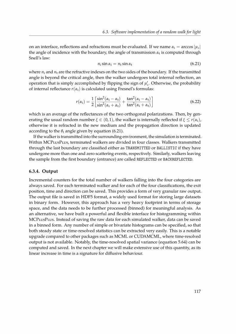
6.3. Software implementation of a random walk for light
on an interface, reflections and refractions must be evaluated. If we name αi = arccos |µz|the angle of incidence with the boundary, the angle of transmission αt is computed throughSnell’s law:
ni sin αi = nt sin αt (6.21)
where ni and nt are the refractive indexes on the two sides of the boundary. If the transmittedangle is beyond the critical angle, then the walker undergoes total internal reflection, anoperation that is simply accomplished by flipping the sign of µ′z. Otherwise, the probabilityof internal reflectance r(αi) is calculated using Fresnel’s formulas:
r(αi) =12
[sin2(αi − αt)
sin2(αi + αt)+
tan2(αi − αt)
tan2(αi + αt)
](6.22)
which is an average of the reflectances of the two orthogonal polarizations. Then, by gen-erating the usual random number ξ ∈ (0, 1), the walker is internally reflected if ξ ≤ r(αi),otherwise it is refracted in the new medium and the propagation direction is updatedaccording to the θt angle given by equation (6.21).
If thewalker is transmitted into the surrounding environment, the simulation is terminated.Within MCPlusPlus, terminated walkers are divided in four classes. Walkers transmittedthrough the last boundary are classified either as TRANSMITTED or BALLISTIC if they haveundergone more than one and zero scattering events, respectively. Similarly, walkers leavingthe sample from the first boundary (entrance) are called REFLECTED or BACKREFLECTED.
6.3.4. Output
Incremental counters for the total number of walkers falling into the four categories arealways saved. For each terminated walker and for each of the four classifications, the exitposition, time and direction can be saved. This provides a form of very granular raw output.The output file is saved in HDF5 format, a widely used format for storing large datasetsin binary form. However, this approach has a very heavy footprint in terms of storagespace, and the data needs to be further processed (binned) for meaningful analysis. Asan alternative, we have built a powerful and flexible interface for histogramming withinMCPlusPlus. Instead of saving the raw data for each simulated walker, data can be savedin a binned form. Any number of simple or bivariate histograms can be specified, so thatboth steady state or time-resolved statistics can be extracted very easily. This is a notableupgrade compared to other packages such asMCML or CUDAMCML, where time-resolvedoutput is not available. Notably, the time-resolved spatial variance (equation 5.64) can becomputed and saved. In the next chapter we will make extensive use of this quantity, as itslinear increase in time is a signature for diffusive behaviour.
117


Chapter 7.
Deducing effective light transport parametersin optically thin systems
In this study we tackle the so-called inverse problem of light transport in thin slabs, i.e. the de-termination of the microscopic properties at the base of light propagation (such as the scatteringmean free path ls and the scattering anisotropy g) starting from macroscopic ensemble observables.We investigate light transport through a single thin slab of scattering material by focusing on twoexperimental observables. The decay time of the transmitted intensity in response to a light pulseimpinging on the slab has long been accessible experimentally and used to determine the diffusionproperties. Notably, we also consider another robust observable which became experimentally ac-cessible with modern optical gating techniques, i.e. the Mean Square Width (MSW) growth of thespatial profile of the transmitted pulse. Such quantity grows linearly in time in a diffusive regime,and is inherently robust since by definition it does not depend on absorption and its slope is directlyrelated to the diffusion coefficient. We build a large database of these two observables over a broadparameter space in terms of ls, g and optical thickness (ranging from 1 to 10). With the combineduse of these two macroscopic quantities, which are both experimentally accessible, we develop alook-up table routine that allows us to retrieve the microscopic transport properties such as ls andg in the relevant case of a thin slab. The results presented here are in publication in New Journalof Physics [32].
7.1. Introduction
Studying light propagation through matter has provided powerful and versatile tools toinvestigate the optical properties of materials in different fields of science and technology.Indeed, predicting how light is scattered by a turbid medium allows one to relate theobserved experimental parameters, measured by shining light through a specimen of agiven material, to the microscopic structural and chemical properties. For example, it wasrecently demonstrated how the exceptionally white brightness of the body of Cyphochilus —a kind of beetle common in South Asia — originates from an optimized anisotropy of chitinnetworks acting as a dense scattering medium for light [33]. These networks are to be foundin the beetle’s scales which are just a few micrometers thick, providing an example of hownature efficiently managed to engineer whiteness. Thus, those findings are interesting notonly from the point of view of natural science, but also as a source of inspiration for thedesign of new materials. Material science is indeed one branch that can undoubtedly benefit
119

Chapter 7. Deducing effective light transport parameters in optically thin systems
from a thorough knowledge of the microscopic properties of matter, which as said can beprobed by passing light through the particular material under investigation. Also, light canbe used as a non-invasive diagnostic tool, e.g. for probing thin layers of paint in a painting.An important field of application, which grew considerably in the past years and is stillgrowing, is that of biomedical optics [8], in which light can be used as a non-destructive toolto quantitatively access the properties of in vivo tissues depending on how it is scattered orabsorbed [34, 35]. From just these few examples, it is clear how solving the so-called inverseproblem — i.e. the determination of the microscopic properties that affect light propagationstarting from macroscopic ensemble observables — is a problem of primary importanceboth from the point of view of fundamental science as well as application-wise. In thischapter we are going to describe the procedure that we have developed to map the observedmacroscopic parameters to a table of simulated observables (namely the Mean SquareWidthslope and the decay time), which allows us to tackle the inverse problem in thin slabs wherethe Diffusion Approximation fails.As we have seen in Chapter 5, the Diffusion Approximation (DA) provides a robust
theoretical framework leading to very simple analytical expressions that describe lighttransport both in space and time. With these, it is possible to solve the inverse problemand retrieve the microscopic parameters. However, the DA comes with some points offailure built-in, as a consequence of the approximations that we have made to derive it. Inparticular, we obtained the DA under the assumption of almost isotropic radiance (5.26),a condition that is truly verified only asymptotically in space and time and progressivelybreaks down if the characteristic scattering length becomes comparable to the thicknessof the slab or to the absorption length. Therefore, the DA is bound to significantly fail formedia whose extension is not large enough to allow the onset of a multiple-scattering regime.This is typical in biomedical optics, since biological materials often naturally come in theform of thin tissues or membranes: ocular fundus [36], vascular walls [37], living epithelialcells [38], skin dermis [39], bone tissue [40], dental enamel [41]. In this cases, in order tohave more accurate results, refined approximations to the Radiative Transport Equationare still actively investigated [42–44], or alternatively a Monte Carlo approach is able toprovide an exact solution for the RTE where the only uncertainty is given by statistical noise.Nevertheless, due to its simplicity and its convenience in characterizing scattering media,the DA still retains a large appeal, and numerous attempts were made to try to extend itsvalidity range in special situations by introducing all sorts of minor modifications [45, 46].Even at its standard formulation derived in Sections 5.5 and 5.6, the DA casts an incrediblysimple prediction on transverse transport: a light beam impinging on a scattering slab willbe transmitted with an enlarged Gaussian profile in space which grows linearly in timeas w2(t) = 4Dt, where the mean square width w2(t) is defined for an arbitrary intensitydistribution I(ρ, t) by equation (5.64), here rewritten for convenience:
w2(t) =
∫ ∞0 ρ2 I(ρ, t)ρ dρ∫ ∞
0 I(ρ, t)ρ dρ(7.1)
120

7.1. Introduction
Experimentally, the evolution in time of the Mean Square Width (MSW) can be measuredfrom a collection of discrete spatio-temporally resolved profiles I(ρ, ti) obtained with opti-cal gating techniques [19, 47]. The slope of its linear growth is predicted by the diffusionapproximation to be determined by the diffusion coefficient D, and the linear increase itselfcan be considered as a signature of diffusion. It is worth remarking how an experimentalobservable based on the mean square width is very robust in its nature, since by definition itis independent from absorption, which cancels out exactly at every ti in (7.1). Additionally,according to the diffusion approximation, the mean square width does not depend on theslab thickness nor on the refractive index contrast between the material and the surround-ing environment. These are unique properties to the mean square width, whereas otherobservables depend critically on boundary conditions, sample size and absorption.
The present study is aimed at characterizing light transport in the infinite slab geometry forthe relevant case of optically thin slabs, a configuration in which the diffusion approximationis expected to be no longer valid. In particular, we perform Monte Carlo simulations over abroad range of optical parameters and test how the DA prediction on transverse transport,i.e. the linear MSW increase, behaves as the optical thickness of the sample decreases. Infact we believe that the simple DA prediction can still be profitably applied in a thin slabgeometry, since boundary and confinement effects are less relevant along the slab’s mainextension where transverse transport occurs. Dealing with thin slabs of course means thatthe vast majority of transmitted light will be ballistic — i.e. light which has undergone anumber of scattering events equal to zero or close to unity — therefore uninteresting for ourpurposes. This represents a challenge also whenmodelling the Radiative Transport Equationby means of Monte Carlo, since in order to keep statistical noise levels to a minimum onehas to simulate an enormous number of photons. By taking into careful considerationtransverse transport and its related observables, our study completes the picture on thebreakdown of the diffusion approximation when moving from the diffusive to the ballisticregime — a transition that has been so far extensively characterized with respect to axialrather than transverse propagation [22, 48–50], relying mostly on the decay time τ as themain observable. Indeed, even when exploiting Monte Carlo modelling, which does notpose any limitation as for the available observables, transverse transport has been largelydisregarded in previous studies, supposedly because it was hardly accessible experimentallybefore the advent of more recent techniques [47]. With a large set of simulated data, wefinally develop a Look-Up Table (LUT) routine as a straightforward tool to solve the inverseproblem in thin slabs, starting from robust experimental observables such as τ and the MSWslope which are independent of absolute intensity measurements. Moreover, as we will seein chapter 8, tackling the problem of transverse transport in a confined geometry is one offundamental interest, as we will show that a multiple-scattering regime can occur even inthin semi-transparent media which are not usually associated with this transport regime.
121
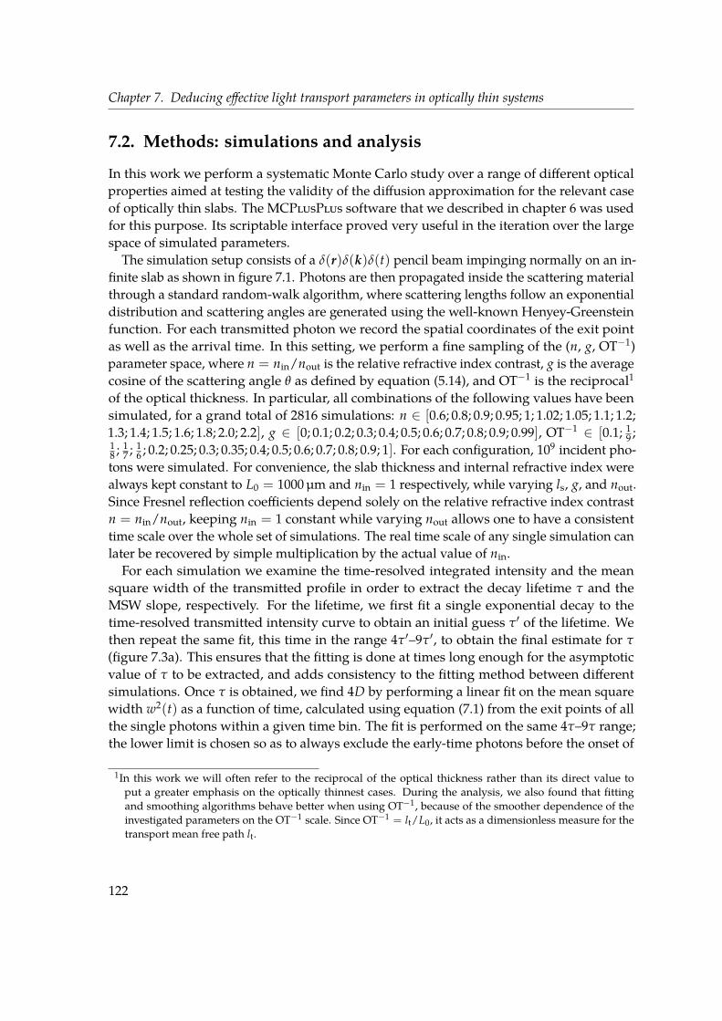
Chapter 7. Deducing effective light transport parameters in optically thin systems
7.2. Methods: simulations and analysis
In this work we perform a systematic Monte Carlo study over a range of different opticalproperties aimed at testing the validity of the diffusion approximation for the relevant caseof optically thin slabs. TheMCPlusPlus software that we described in chapter 6 was usedfor this purpose. Its scriptable interface proved very useful in the iteration over the largespace of simulated parameters.
The simulation setup consists of a δ(r)δ(k)δ(t) pencil beam impinging normally on an in-finite slab as shown in figure 7.1. Photons are then propagated inside the scattering materialthrough a standard random-walk algorithm, where scattering lengths follow an exponentialdistribution and scattering angles are generated using the well-known Henyey-Greensteinfunction. For each transmitted photon we record the spatial coordinates of the exit pointas well as the arrival time. In this setting, we perform a fine sampling of the (n, g, OT−1)parameter space, where n = nin/nout is the relative refractive index contrast, g is the averagecosine of the scattering angle θ as defined by equation (5.14), and OT−1 is the reciprocal1of the optical thickness. In particular, all combinations of the following values have beensimulated, for a grand total of 2816 simulations: n ∈ [0.6; 0.8; 0.9; 0.95; 1; 1.02; 1.05; 1.1; 1.2;1.3; 1.4; 1.5; 1.6; 1.8; 2.0; 2.2], g ∈ [0; 0.1; 0.2; 0.3; 0.4; 0.5; 0.6; 0.7; 0.8; 0.9; 0.99], OT−1 ∈ [0.1; 1
9 ;18 ; 1
7 ; 16 ; 0.2; 0.25; 0.3; 0.35; 0.4; 0.5; 0.6; 0.7; 0.8; 0.9; 1]. For each configuration, 109 incident pho-
tons were simulated. For convenience, the slab thickness and internal refractive index werealways kept constant to L0 = 1000 µm and nin = 1 respectively, while varying ls, g, and nout.Since Fresnel reflection coefficients depend solely on the relative refractive index contrastn = nin/nout, keeping nin = 1 constant while varying nout allows one to have a consistenttime scale over the whole set of simulations. The real time scale of any single simulation canlater be recovered by simple multiplication by the actual value of nin.For each simulation we examine the time-resolved integrated intensity and the mean
square width of the transmitted profile in order to extract the decay lifetime τ and theMSW slope, respectively. For the lifetime, we first fit a single exponential decay to thetime-resolved transmitted intensity curve to obtain an initial guess τ′ of the lifetime. Wethen repeat the same fit, this time in the range 4τ′–9τ′, to obtain the final estimate for τ
(figure 7.3a). This ensures that the fitting is done at times long enough for the asymptoticvalue of τ to be extracted, and adds consistency to the fitting method between differentsimulations. Once τ is obtained, we find 4D by performing a linear fit on the mean squarewidth w2(t) as a function of time, calculated using equation (7.1) from the exit points of allthe single photons within a given time bin. The fit is performed on the same 4τ–9τ range;the lower limit is chosen so as to always exclude the early-time photons before the onset of
1In this work we will often refer to the reciprocal of the optical thickness rather than its direct value toput a greater emphasis on the optically thinnest cases. During the analysis, we also found that fittingand smoothing algorithms behave better when using OT−1, because of the smoother dependence of theinvestigated parameters on the OT−1 scale. Since OT−1 = lt/L0, it acts as a dimensionless measure for thetransport mean free path lt.
122

7.2. Methods: simulations and analysis
30 ps 60 ps 90 ps 120 ps
ρ
I(ρ,t)
0 50 100
t(ps)
w2 (
t)/
l2 t(a
.u.)
0 50 100
t(ps)
log
T(t)
(a.u
.)
Figure 7.1.: Left panel: sketch of the investigated configuration. A pencil beam impinges on aninfinite slab, and can undergo multiple scattering even in thin slabs (as discussed in greater detail inchapter 8). At each time slice, the transmitted profile is approximately Gaussian. Its mean squarewidth w2(t) grows linearly in time (central panel) while the spatially integrated transmitted intensityT(t) falls exponentially (right panel).
the diffusive regime, while the upper limit is to avoid the noise found at very long times dueto insufficient statistics (figure 7.2a). As previously specified, mean square width values areexactly independent of absorption, which has thus been excluded from the simulations.It is worth explaining why it is appropriate to use the decay time as a time unit for the
mean square width evolution, since the former is mainly determined by transport propertiesalong the slab thickness, while the latter occurs mainly in-plane. A time range based onτ actually provides a convenient way of defining a consistent, self-tuning fitting windowacross the whole dataset. This simple choice is also advocated under practical reasons,since the decay time is undoubtedly the actual temporal unit that eventually dictates —both in real and numerical experiments — the signal-to-noise ratio. In this respect, everydiffusion coefficient within our simulated phase space has been determined under equalnoise conditions. No less important, limiting our investigation to a long-time window isalso relevant under a more technical point of view: for all practical purposes, the specificchoice of both the spatial source distribution and the phase function becomes negligible.
Each simulated point in the (n, g, OT−1) parameter space defines a discrete grid. Followingthe analysis protocol described above, the extracted values of D and τ can be assigned to eachpoint of the grid. In other words, we have two sets of four-dimensional data, that are bestarranged in the form of a hypersurface as shown in figures 7.2b and 7.3b. Instead of their rawvalues, we plot the deviations from the prediction cast by the diffusive approximation. Theobtained values for D, evaluated as 1/4 of the variance slope, are divided by the predictedvalue (equation 5.65)
DDA =13
ltc (7.2)
Accordingly, values for τ are compared to the expression that we found within the diffusive
123
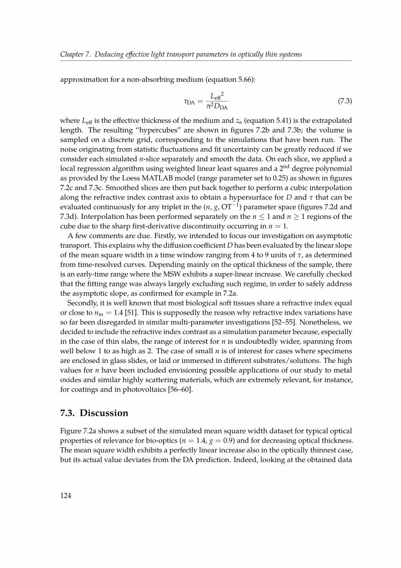
Chapter 7. Deducing effective light transport parameters in optically thin systems
approximation for a non-absorbing medium (equation 5.66):
τDA =Leff
2
π2DDA(7.3)
where Leff is the effective thickness of the medium and ze (equation 5.41) is the extrapolatedlength. The resulting “hypercubes” are shown in figures 7.2b and 7.3b; the volume issampled on a discrete grid, corresponding to the simulations that have been run. Thenoise originating from statistic fluctuations and fit uncertainty can be greatly reduced if weconsider each simulated n-slice separately and smooth the data. On each slice, we applied alocal regression algorithm using weighted linear least squares and a 2nd degree polynomialas provided by the Loess MATLAB model (range parameter set to 0.25) as shown in figures7.2c and 7.3c. Smoothed slices are then put back together to perform a cubic interpolationalong the refractive index contrast axis to obtain a hypersurface for D and τ that can beevaluated continuously for any triplet in the (n, g, OT−1) parameter space (figures 7.2d and7.3d). Interpolation has been performed separately on the n ≤ 1 and n ≥ 1 regions of thecube due to the sharp first-derivative discontinuity occurring in n = 1.A few comments are due. Firstly, we intended to focus our investigation on asymptotic
transport. This explainswhy the diffusion coefficient D has been evaluated by the linear slopeof the mean square width in a time window ranging from 4 to 9 units of τ, as determinedfrom time-resolved curves. Depending mainly on the optical thickness of the sample, thereis an early-time range where the MSW exhibits a super-linear increase. We carefully checkedthat the fitting range was always largely excluding such regime, in order to safely addressthe asymptotic slope, as confirmed for example in 7.2a.Secondly, it is well known that most biological soft tissues share a refractive index equal
or close to nin = 1.4 [51]. This is supposedly the reason why refractive index variations haveso far been disregarded in similar multi-parameter investigations [52–55]. Nonetheless, wedecided to include the refractive index contrast as a simulation parameter because, especiallyin the case of thin slabs, the range of interest for n is undoubtedly wider, spanning fromwell below 1 to as high as 2. The case of small n is of interest for cases where specimensare enclosed in glass slides, or laid or immersed in different substrates/solutions. The highvalues for n have been included envisioning possible applications of our study to metaloxides and similar highly scattering materials, which are extremely relevant, for instance,for coatings and in photovoltaics [56–60].
7.3. Discussion
Figure 7.2a shows a subset of the simulated mean square width dataset for typical opticalproperties of relevance for bio-optics (n = 1.4, g = 0.9) and for decreasing optical thickness.The mean square width exhibits a perfectly linear increase also in the optically thinnest case,but its actual value deviates from the DA prediction. Indeed, looking at the obtained data
124

7.3. Discussion
(figure 7.2d), two features are immediately noticeable. First of all, the diffusion approxi-mation appears to always underestimate the actual spreading rate, of course recoveringagreement for higher optical thicknesses as expected. A second, finer feature occurs inthe close proximity of n = 1, particularly evident at low g and OT values. Both these fea-tures arise from the interplay between geometric and boundary conditions. In particular,in chapter 8 we will see that the presence of internal reflections in a thin layer geometryhelps to selectively hold inside the slab those photons that happen to draw statisticallylonger steps. For the moment, we stress that the mean square width slope exhibits a distinctpattern of characteristic deviations from the diffusion approximation, which can therefore beexploited as a tool to unambiguously retrieve the intrinsic microscopic transport propertiesof a given sample. In particular, we notice a subtle dependence on g that, however small,can be profitably used to finally access the angular statistics of the scattering process.Looking at the decay times (figure 7.3d), it is worth highlighting two main differences
from the results described above for the mean square width slope. First of all, the observeddecay times deviate more from the values predicted by the diffusive approximation, as theycan take values as low as 20% of what is predicted by the DA (for the highest values of gand n). It is indeed known that refractive index contrasts greater than one (n > 1) are harderto be taken into account, even when appropriate boundary conditions are considered andeven at high OT [50]. Secondly, we note that deviations in both directions are possible, sincethe τ/τDA ratio can take values that are both greater and smaller than 1. We here stress theimportance of an accurate and precise modelling of the index contrast, which we think hasbeen often overlooked, for example when an averaged contrast is used to model asymmetricexperimental configurations [44, 61].
By combining the two investigated observables, i.e. the mean square width slope and thedecay time, some unique insight on the effects of absorption can be gained, as we will showin the next section. On one hand, the effects of absorption cancel out exactly in w2(t), whilethe asymptotic decay time is expected to shift exactly to
1τ→ 1
τ+ µav (7.4)
τ being the decay time in the non-absorbing case. The presence of absorption is oftenregarded as the source of numerous problems, since both scattering and absorption competeto the depletion of specific intensity from a given position, time and direction (an effectsometimes referred to as absorption-to-scattering cross-talk, see equation 5.20). This is oftenconsidered a major hindrance in the correct determination of transport properties [21, 62–66].Besides that, having a weakly absorbing medium — i.e. one where µa µ′s — is oftenquoted as a required condition for the diffusive theory to hold. Indeed, the diffusive regimecoincides with a multiple-scattering regime, in which long trajectories dominantly shapethe transport properties. In the presence of increasing absorption though, longer paths areselectively more and more penalized [5]. Diffusion theory therefore progressively breaksdown, since transport becomes dominated by short trajectories with few scattering events.
125
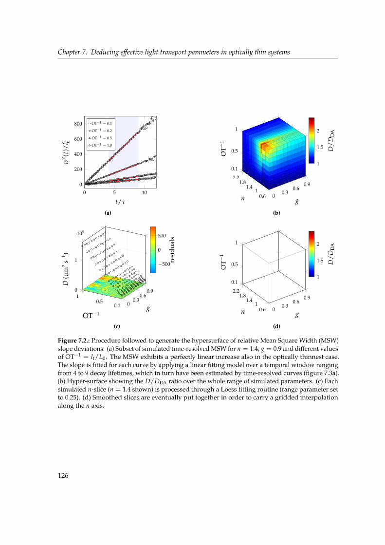
Chapter 7. Deducing effective light transport parameters in optically thin systems
0 5 10
0
200
400
600
800
t/τ
w2 (
t)/
l2 t
OT−1 = 0.1
OT−1 = 0.2
OT−1 = 0.5
OT−1 = 1.0
(a)
00.3
0.60.9
0.61
1.41.8
2.2
0.1
0.5
1
gn
OT−
1
1
1.5
2
D/
DD
A
(b)
00.3
0.60.9
0.10.5
10
1
·105
gOT−1
D(µ
m2
s−1)
−500
0
500
resi
dual
s
(c)
00.3
0.60.9
0.61
1.41.8
2.2
0.1
0.5
1
gn
OT−
1
1
1.5
2
D/
DD
A(d)
Figure 7.2.: Procedure followed to generate the hypersurface of relative Mean Square Width (MSW)slope deviations. (a) Subset of simulated time-resolvedMSW for n = 1.4, g = 0.9 and different valuesof OT−1 = lt/L0. The MSW exhibits a perfectly linear increase also in the optically thinnest case.The slope is fitted for each curve by applying a linear fitting model over a temporal window rangingfrom 4 to 9 decay lifetimes, which in turn have been estimated by time-resolved curves (figure 7.3a).(b) Hyper-surface showing the D/DDA ratio over the whole range of simulated parameters. (c) Eachsimulated n-slice (n = 1.4 shown) is processed through a Loess fitting routine (range parameter setto 0.25). (d) Smoothed slices are eventually put together in order to carry a gridded interpolationalong the n axis.
126
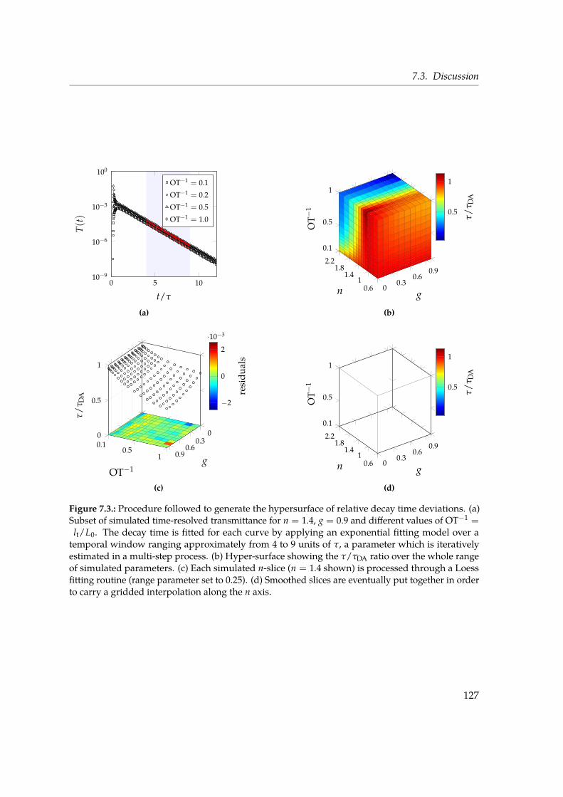
7.3. Discussion
0 5 1010−9
10−6
10−3
100
t/τ
T(t)
OT−1 = 0.1
OT−1 = 0.2
OT−1 = 0.5
OT−1 = 1.0
(a)
00.3
0.60.9
0.61
1.41.8
2.2
0.1
0.5
1
gn
OT−
1 0.5
1
τ/
τ DA
(b)
00.3
0.60.9
0.10.5
1
0
0.5
1
gOT−1
τ/
τ DA
−2
0
2
·10−3
resi
dual
s
(c)
00.3
0.60.9
0.61
1.41.8
2.2
0.1
0.5
1
gn
OT−
1 0.5
1
τ/
τ DA
(d)
Figure 7.3.: Procedure followed to generate the hypersurface of relative decay time deviations. (a)Subset of simulated time-resolved transmittance for n = 1.4, g = 0.9 and different values of OT−1 =lt/L0. The decay time is fitted for each curve by applying an exponential fitting model over atemporal window ranging approximately from 4 to 9 units of τ, a parameter which is iterativelyestimated in a multi-step process. (b) Hyper-surface showing the τ/τDA ratio over the whole rangeof simulated parameters. (c) Each simulated n-slice (n = 1.4 shown) is processed through a Loessfitting routine (range parameter set to 0.25). (d) Smoothed slices are eventually put together in orderto carry a gridded interpolation along the n axis.
127

Chapter 7. Deducing effective light transport parameters in optically thin systems
The task of assessing the presence of absorption has been to date a very challenging one, butthe use of absorption-independent observables such as the rate of the mean square widthgrowth can help disentangle its role. For this reason, techniques capable of providing directaccess to the mean square width recently stimulated a great deal of interest [67–69], giventhe absorption-independent nature of the variance expansion. The full potential of MSWmeasuring techniques probably has yet to be fully unravelled, and will eventually play a keyrole among the most accurate characterization techniques for both scattering and absorptionproperties.
On a last remark, we note that a vast literature on the validity range of the diffusionapproximation in the time domain has been produced [22, 48–50, 70–73], but a compre-hensive understanding of the interplay between optical thickness, refractive index contrastand absorption is still a debated topic. It is a commonly accepted fact that the diffusionapproximation fails gradually with decreasing optical thickness, with OT = 8 being custom-arily considered as the lower threshold under which the introduced error starts to becomenon negligible [50]. Nevertheless, in a recent work a non-absorbing slab with n ≈ 1.5 andOT = 8 was investigated experimentally, and a transmittance lifetime was found such thatthe diffusion approximation is unable to provide any real solution for τ [74]. This suggeststhat the breakdown of the diffusion approximation might step in abruptly depending onthe interplay between different parameters other than the optical thickness. In the followingsection we will show that the decay lifetime and mean square width expansion that wereexperimentally observed for that sample are in perfect agreement with our simulations. Infact, they can even be triangulated within our simulated dataset, by accessing the simulateddata following a Look-Up Table (LUT) approach.
7.4. Look-up table approach
In the introduction to this chapter we emphasized how solving the so-called inverse problem— i.e. the retrieval of the properties that govern light transport at the microscopic scale —is of great importance both fundamentally and application-wise. In the past years, thanksto the broad availability of high computing power, Monte Carlo methods have become awidely used tool to tackle the inverse problem. Broadly speaking, two main approaches areused: Monte Carlo fitting and Look-Up Table (LUT) routines.
In the first case, the forward problem is iteratively solved by means of Monte Carlo simula-tions while varying the transport parameters, until convergence with the experimental datais reached. This approach is computationally demanding, therefore existing implementa-tions typically take advantage of rescaling properties of the Radiative Transport Equation toadapt a limited set of pre-simulatedMonte Carlo data to the experimental measurements [36,49, 52, 75–79]. Unfortunately, this too presents some challenges, since rescaling must be doneon a single photon basis to limit the occurrence of “scaling artefacts”, thus requiring to storeeach exit time and position separately [77, 78]. Furthermore, improper binning strategies
128

7.4. Look-up table approach
are a possible source of artefacts, requiring complicated binning criteria to be devised [79].Finally, it is worth noting that while a single dimensionless Monte Carlo simulation fora semi-infinite geometry can be easily rescaled, for finite-thickness geometries (slabs) thecomputational burden increases quickly, since different scattering mean free paths valuesmust be simulated separately. This is probably the reason why only few examples can befound in the literature dealing with this configuration [52].LUT routines are instead based on a database of pre-simulated configurations that is
queried to solve the inverse problem. In this case, the computational burden is a one-timeeffort, concentrated in the construction of a look-up tablewhich can be later straightforwardlyaccessed at no computational cost. Several LUTmethods can be found in the literature, basedon both experimental [54] and simulated data [53, 55, 80–85]. The typical scalar parameterson which these routines rely are the total amount of transmitted/ballistic/reflected lightfrom a slab, which are linked to the transport properties. This triplet of observables, oftenreferred to as Ttot, Tcoll and Rtot, has been extensively exploited to retrieve optical parametersthrough Monte Carlo-based LUT routines [53, 55, 80–85]. Unfortunately, resorting to thiskind of observables brings about some problems. First of all, the mentioned parameters areall absolute quantities, therefore not easily measured [53, 83] and prone to unpredictablesystematic errors [85]. Secondly, for thin samples — which are the focus of this and otherstudies aimed at providing an alternative where the DA approximation breaks down —the importance of these observables is greatly reduced [36]: indeed, for thin systems theirvalues become dominated by light that has been either specularly reflected or ballisticallytransmitted through the sample, thus carrying very little information about the materialproperties.
Taking advantage of the large set of simulations that we have performed, we propose alook-up table (LUT) routine to demonstrate how the combined use of the mean square widthslope and the decay lifetime can be very effective at tracking down the microscopic transportproperties. The advantages originating from the use of these observables are manifold. Firstof all they are very robust, since they are free from any absolute intensity measurement andthey are evaluated well into the multiple-scattering regime; therefore there’s no need tocalibrate the source, the detector or to know exactly the excitation intensity. Also, knowledgeof the temporal response function or of the actual size of the excitation spot is not required,since both τ and w2(t) are asymptotic quantities. Nor is the precise determination of theorigin of the time axis (i.e. the exact time of pulse injection), which instead is critical inother measurements; indeed both the decay lifetime and the linear increase of the meansquare width do not exhibit any critical dependence on the exact delay at which they aredetermined, provided that it is sufficiently large. Besides the robustness of the observablesthat we have considered, a LUT approach has on its own some advantages over MonteCarlo fitting routines. Indeed, retrieval of data from a LUT is very fast, since no iterativeprocedure is involved, therefore a LUT is more suitable for real-time solving of the inverseproblem. A LUT based on our two scalar parameters can be rescaled easily; since the scalar
129

Chapter 7. Deducing effective light transport parameters in optically thin systems
parameters are extracted with their proper original binning, rescaling does not introduceany binning-related artefact. Finally, our LUT notably does not include absorption; thereforethe computational burden that this poses on Monte Carlo simulations can be reasonablyhandled, since we are dealing with a simulation phase space of reduced dimensionality.Actually, the fact that there even is no need to add absorption after the simulation is run,means that it is also not necessary to store exit times and positions on a single-photon basis;therefore, the LUT footprint in terms of the total size of data that has to be stored is kept tothe minimum.For the sake of simplicity, our present Monte Carlo-LUT demonstration is limited to the
retrieval of the following pairs of transport parameters:
• lt and g assuming that absorption is known, or
• lt and µa assuming that g is known.
The latter is a realistic and common assumption in similar works, especially those involvingbiological samples [52, 53, 76]. The effective refractive index n and the thickness of thesample L are also expected as input parameters. The LUT that we have developed, whichwe are now going to describe, can be queried online via a dedicated interface at this address:http://www.lens.unifi.it/quantum-nanophotonics/mcplusplus/lut/.To illustrate the steps involved in the look-up table routine (figure 7.4), we first test the
retrieval procedure against two simulated samples, and later on real experimental data. Wesimulate a set of parameters that are not included in the database on which the LUT is built;specifically, we consider two samples with L = 1.3 mm, n = 1.38, g = 0.95, ls = 45 µm andµa respectively equal to 0.2mm−1 and 0mm−1 (i.e. no absorption). From these simulationswe extract the mean square width slope and the decay time, which we use as inputs for theLUT routine to find what we pretend to be the unknown values.The first step of the LUT procedure involves rescaling of the mean square width and
lifetime hypersurfaces. Rescaling must be done both in space and time to match the targetthickness and refractive index. The original simulations were performed for a sample ofthickness L0 = 1 mm and unitary internal refractive index; dimensional analysis shows thateventually the mean square width and lifetime hypersurfaces are to be rescaled by L/(L0nin)
and ninL/L0 respectively.Let us consider the first case of a medium with unknown scattering mean free path and
absorption coefficient, but known g. After proper rescaling of the continuously interpolatedversion of the mean square width hypersurface (figure 7.2d), we can slice the data at thegiven refractive index contrast n. The obtained two-dimensional surface will feature aniso-level curve corresponding to themeasuredmean square width slope, whichwill basicallygive the expected OT−1, i.e. lt, in a completely absorption-independent way. For the testsample described above, fitting the simulated mean square width values yields a slopeof 337 750µm2 ps−1, i.e. D = 84 437 µm2 ps−1. By intersecting this iso-level curve with thesimulated value of g = 0.95 (which we take as known), we eventually retrieve the best OT−1
130

7.4. Look-up table approach
0.2
0.3
0.4
0.5
0.6
0.7
0.80.91
1.11.21.3
0 0.3 0.6 0.90.1
0.4
0.7
1
g
OT−
1
0.5
1
·105
D(µ
m2
ps−1
)
(a)
0 50 100 15010−11
10−8
10−5
t (ps)T(t)
sim. experimentfitno absorption
(b)
22
23
23
23
24
24
25
24 2425 25
26
26 26
27
27 2728 28
28
29 2930 30
29
31 31
30
31
0 0.3 0.6 0.90.1
0.4
0.7
1
g
OT−
1
22
24
26
28
30
τ(p
s)
(c)
0 0.2 0.4 0.6 0.8 1
22
24
26
g
τ(ps)
interp. τ on iso-D curvespline fit
(d)
Figure 7.4.: Demonstration of the MC-LUT routine. (a-b) Retrieving lt and µa with known g. Themeasured value of D is used to draw an iso-D curve (dashed line in panel a) on the proper n sliceextracted from the hypersurface shown in figure 7.2d. OT−1 is found by intersecting the iso-Dcurve with the value of g, which is assumed to be known. Once OT−1 is determined, the expectedabsorption-free lifetime value is retrieved from the hypersurface of figure 7.3d is plotted as a dashedblue line in panel b; comparison with the experimental lifetime yields µa. (c-d) Retrieving lt and gwith known µa. Intersecting iso-D and iso-τ curves yields g (panel c and d), which can then be usedas in the previous case.
131

Chapter 7. Deducing effective light transport parameters in optically thin systems
estimate (figure 7.4a). Nonetheless, even if the scattering anisotropy is not known a priori,plugging reasonably bounded values into the routine helps getting an estimate of how anuncertainty on g spreads over lt and eventually µa. Once that also OT−1 is determined, it issufficient to read the expected absorption-free lifetime value stored in τ(n,OT−1, g) (shownin figure 7.4b as a dashed blue line) from the interpolated lifetime hypersurface (figure 7.3d)and compare it directly to the measured value: the discrepancy between their reciprocalvalues will directly give µac/nin through equation (7.4). Fitting the simulated transmittedintensity decay yields a decay time of 11.234 ps, and we finally retrieve µa = 0.1997 mm−1
and lt = 897 µm, to be compared with the initial values µa = 0.2 mm−1 (δx ≈ −1.5× 10⁻³)and lt = ls/(1− g) = 45 µm/0.05 = 900 µm (δx ≈ −3× 10⁻³).
The second implementation of our routine allows to retrieve lt and g assuming that µa isknown. A common case is that of vanishing absorption, which is often encountered whenstudying for example metal oxide powders with NIR radiation. Since D is not affected byabsorption, we reconsider the same iso-D curve of figure 7.4a which we replot in figure 7.4c.Superimposing this curve over the τ(n = 1.38) surface and its experimental iso-τ curve at21.936 ps (dashed line in figure 7.4c) finally gives the estimated g parameter — for exampleby means of spline interpolation over a discrete set of (OT−1, g) pairs evaluated on the iso-Dcurve (figure 7.4d) — which can then be used proceeding as in the previous case. We findlt = 897 µm and g = 0.938 (δx ≈ −1.2× 10⁻²).We now test our LUT against recent experimental data, where mean square width mea-
surements are obtained by means of an ultrafast optical gating technique. Pattelli et al. [74]recently highlighted the robustness of the mean square width as a valuable experimentalobservable for the retrieval of the microscopic transport parameters. In that work, the au-thors consider a homogeneous isotropic sample made of TiO2 nanoparticles (g = 0.6, withvanishing absorption at the working wavelength of 810 nm) embedded in a polymer matrix;sample thickness was measured to be 203µm and the average refractive index at the workingwavelength is 1.52, close to that of many biological tissues. The authors found an experi-mental lifetime and a mean square width slope of 6.01 ps and 6984µm2 ps−1 respectively,for which the diffusion approximation was unable to provide any real solution all. They alsofound a value of lt = 25.5 µm with a brute-force Monte Carlo inversion procedure againstthe experimental data, involving the simulation of many combinations of optical parameters(what we defined above as Monte Carlo fitting). Here, by feeding the same experimentalparameters into our look-up table routine, we instantly find a value of lt = 25.7 µm, in goodagreement with the value reported in the paper.Evaluation of errors should be performed on a wide range of parameters, both from
simulations and experimental data, which is beyond the scope of this work. Nonetheless wenote that, especially at lower thickness where the diffusion approximation is bound to fail,our routine offers accurate retrieving capabilities as compared to other slab-geometry fittingand/or LUT approaches [52].
132

7.5. Conclusions
7.5. Conclusions
By means of Monte Carlo simulations, we have studied the radiative transfer problem inthe infinitely extended slab geometry. The numerical solutions that we obtain are com-pared to the predictions cast by diffusion theory. The peculiarity of this study is that bothtransverse and axial transport are addressed, using the mean square width growth rate andthe decay time of the spatially integrated transmitted intensity as the respective figures ofmerit. These two observables, measured at late times, provide valuable insight on lighttransport properties well into the diffusive regime. The mean square width growth rate isof particular interest since, within the diffusion approximation, it depends solely on thediffusion coefficient, as opposed to other time-resolved observables where also the thicknessand refractive index contrast usually play a critical role.
Our investigation provides a complete characterization of how the diffusive approximationgradually fails over a range of optical thicknesses from 10 to 1. An extensive database ofmean squarewidth slopes and decay lifetimeswas built, by systematically performingMonteCarlo simulations over a three-dimensional parameter space consisting of the refractiveindex contrast n, the scattering anisotropy g and scattering mean free path ls.As regards the mean square width expansion rate, our results deviate from the simple
diffusion approximation prediction especially at low optical thicknesses and scatteringanisotropy, always in the form of an underestimation of the actual rate. Notably, whenconsidering the case of high scattering anisotropywhich is most relevant in many biomedicalapplications, the magnitude of the observed deviation remains limited even at low opticalthicknesses. Decay times instead deviate significantly even when extrapolated boundaryconditions are included; in this case the diffusion approximation can both underestimate oroverestimate the retrieved value.
Taking advantage of the large simulated dataset, we presented a look-up table (LUT) basedon the combination of the decay time and mean square width slope as input parameters,which offer a series of relevant advantages over existing LUT solutions. Prominently, theirexperimental evaluation does not imply any absolute intensity measurement nor precisedetermination of the origin of the time axis. On the contrary the observables that we haveused are inherently precise and robust, since their scalar value is extracted by fitting multiplepoints of a curve. Finally, we have tested the usefulness of our LUT strategy against realexperimental measurements, by showing how microscopic transport properties could beinstantly retrieved for a notable case in which no solution could be foundwithin the diffusiveapproximation.
As a last point, we note that extensions of the presented LUT routine are of course possible.At least a third input observable in addition to the decay time and the mean square widthslope needs to be known in order to retrieve simultaneously all three transport parametersat once from an unknown medium. A possible candidate could be represented by theasymptotic slope of a steady state profile, which should exhibit an appreciable dependenceon g at lower optical thicknesses. Other relative parameters could be exploited, taking
133

Chapter 7. Deducing effective light transport parameters in optically thin systems
advantage of their g dependence, such as the rising time of the time-resolved decay curve[22]. To sum up, look-up table methods are very general in their nature and consequentlycan be profitably applied in a number of practical use cases. Of course, in order to tacklemore complex geometries (e.g. multilayered or anisotropic slabs) more observables areneeded. Nonetheless we believe that, whenever possible, mean square width and decaytime measurements should always be preferred and included in every LUT-based retrievalroutine, thanks to their intrinsic robustness.
134

Chapter 8.
Diffusion of light in thin slabs
In this chapter we study diffusion of light in thin slabs with a particular focus on transverse trans-port. Light diffusion is usually associated with thick, opaque media. Indeed, multiple scatteringis necessary for the onset of the diffusive regime and such condition is generally not met in almosttransparent media. However, as far as in plane propagation is concerned, transport is unboundedand will eventually become diffusive provided that sufficiently long times are considered. By meansof Monte Carlo simulations, we characterise this almost two-dimensional asymptotic diffusive regimethat sets in even for optically thin slabs (OT = 1) making again extensive use of the mean squarewidth growth in time. Even at such low optical thickness, we find a signature of diffusive behaviourin the linear increase of the mean square width slope with time, which however obviously deviatesfrom the prediction cast by the Diffusion Approximation. We show that geometric and boundaryconditions, such as the refractive index contrast, play an active role in redefining the very asymptoticvalue of the diffusion coefficient by directly modifying the statistical distributions underlying lighttransport in a scattering medium.
8.1. Introduction
DuringWorldWar II, AbrahamWald (1902–1950) was working as a member of the StatisticalResearch Group (Columbia University) when he was asked to estimate the vulnerabilityof military aircraft, so that reinforcement strategies could be devised in order to minimizelosses [86, 87]. A previous study by the Center for Naval Analyses, based on the examinationof returned aircraft, had erroneously come to the conclusion that armour should have beenadded to those parts of the aircraft that were damaged the most. Wald instead noted thatthe analysed population was strongly biased, since it relied solely on the data coming fromthe survived aircraft, while there was no means to assess the damage of those aircraft thathad been taken down. However, he was able to realize that the observed population wasnonetheless providing valuable information. In fact, Wald proposed that protections shouldinstead be added to those parts of the aircraft that were not hit, since the fact alone that theplane was able to return meant that it could withstand that kind of damage, i.e. the damagedparts were not critical.
This anecdote helps with introducing the statistical study that we describe in this chapter.Here we investigate light transport in optically thin slabs by focusing our attention onphotons that have “survived” long times inside the sample, and we show that they carry agreat deal of information about the microscopic transport properties of the material. When
135

Chapter 8. Diffusion of light in thin slabs
dealing with optically thin systems, one is faced with the problem that the vast majority oftransmitted light is ballistic or quasi-ballistic, i.e. it is immediately “lost” after zero or onlya few scattering events. Vice versa, those very few photons that instead happen to spendlonger times inside the scattering material will carry a signature of those conditions thatallowed their survival or, equivalently, prevented their early loss.In the previous chapter we numerically investigated how the predictions cast by the
Diffusion Approximation (DA) deviate from the “exact” results obtained by means of MonteCarlo (MC) simulations when optically thin samples are considered. Here, we use MonteCarlo simulations to investigate diffusive behaviour in the thin slab geometry, with a partic-ular focus on transverse transport. Light diffusion is usually associated with thick, opaquemedia, since the onset of multiple scattering is a necessary condition for diffusive behaviour.Conversely, such condition is generally not met in almost transparent media. Nonetheless,as far as in-plane transport is concerned, a multiple-scattering regime can occur even whenthin systems are considered [88]. Indeed, in an infinitely extended slab, transverse propa-gation is unbounded, and will eventually become diffusive at sufficiently long times. Inthis chapter we will specifically focus on this almost two-dimensional asymptotic diffusiveregime. While MC simulations are continuously contributing to unveiling the peculiarphysics that governs light transport in complex media such as heterogeneous or anisotropicmaterials [89, 90], our findings show that our comprehension of way simpler systems sucha homogeneous, isotropic single slab is still incomplete. For example, we show that evena minute tuning in the refractive index contrast allows to sensibly modify the long timebehaviour of semitransparent slabs.
8.2. Transport in a thin slab geometry
In this study we will make again extensive use of the Mean Square Width (MSW):
w2(t) =
∫ ∞0 ρ2 I(ρ, t)ρ dρ∫ ∞
0 I(ρ, t)ρ dρ(8.1)
where I(ρ, t) is the transmitted intensity as a function of time and of the distance fromthe slab axis ρ. We mentioned already many reasons which make the Mean Square Widthan interesting quantity. It is completely independent from absorption, which cancels outexactly at any time [68], and within the simple diffusion approximation it curiously doesnot depend on the slab thickness and its refractive index contrast. In the previous chapterwe found that the mean square width growth in time is remarkably linear — after a shortsuperlinear transient — over the whole range of investigated optical parameters, even at anoptical thickness as low as 1. This can be considered as a signature of diffusive behaviour.Although linear, its slope of course deviates from the simple prediction cast by diffusiontheory, according to which w2(t) = 4DDAt.
136

8.2. Transport in a thin slab geometry
1 1.5 21
1.5
2
2.5
n = nin/nout
D/
DD
A
g = 0g = 0.3g = 0.6g = 0.9
(a)
0 5 10 15
0
50
100
t/τ
w2 (
t)/
l2 t
n = 1.0n = 1.016n = 1.1
(b)
Figure 8.1.: (a) Crosscuts along different values of g of the simulated hyper-surface of figure 7.2b, takenat lt = L0 = 1 mm (OT = 1). For each point, the MSW slope has been evaluated from a simulation of1010 photons. The introduction of a small amount of boundary reflections appears to enhance in-planediffusion remarkably. A subset of parameters (black filled dots) where the effect is more dramaticis further investigated separately, by collecting a much larger statistics. (b) MSW growth for the threedifferent configurations highlighted in panel (a). Linear fits are performed excluding the range t < 4τ.
1 1.5 2
0.5
1
n = nin/nout
τ/
τ DA
g = 0g = 0.3g = 0.6g = 0.9
(a)
0 0.5 1
10
15
20
25
OT−1
τ/
n in(ps)
10 8 4 3 2 1OT
n = 1.1 fitn = 1.4 DA
(b)
Figure 8.2.: (a) Decay time relative deviations at OT = 1 showing crosscuts on g from the hypersurfaceof figure 7.3. The ratio can clearly go above 1 for specific values of n, especially at low g values. Thedependence of τ on OT for the two values highlighted as black filled circles is shown in panel (b),along with the DA prediction and a higher order fit. The DA can both oversetimate (red shaded area)or underestimate (blue shaded area) the simulated value.
137

Chapter 8. Diffusion of light in thin slabs
Considering again the simulations performed in the previous chapter, let us focus onthe case OT = 1. Figure 8.1a shows a subset of the diffusion coefficients obtained from thesimulated mean square width slopes, as extracted from the hypersurface of figure 7.2b forOT = 1. High deviations are obviously expected for such a low optical thickness. However,it is somewhat unexpected that the highest deviations occur in the proximity of n = 1,since the index-matching condition is sometimes quoted as a safer configuration for thediffusion approximation [22]. While this might be true under various circumstances, from anexperimental point of view the typical attempts to approximately index-match a thin samplewithin a reference material might more likely introduce an error rather than neutralize it,since apparently it’s the very smallest index mismatch that results in the strongest deviationsfrom the theory. The relative deviations are always in the form of an overestimation of thediffusion coefficient and they approach unity for increasing optical thickness, thus recoveringthe diffusive prediction as expected.
A possible, intuitive explanation for this nontrivial trend can be found by considering thed-dimensional modelling of diffusion as a randomwalk process. According to the derivationoutlined in section 5.7, given any arbitrary step length distribution P(l) with finite moments〈l〉 and 〈l2〉, the diffusion coefficient can be written as (equation 5.84)
D =1
2dv⟨l2⟩
〈l〉 =1d
vlt (8.2)
where the last equality holds for an exponential step length distribution with average steplength lt. As the optical thickness of the simulated slab decreases, transport occurs in anincreasingly planar geometry. Therefore the perceived dimensionality of the environment,d, drifts from 3 to 2. Hence, as suggested by the above equation, the effective diffusioncoefficient D as inferred from the mean square width slope might be up to 3/2 times higherthan its bulk nominal value. The perceived environment dimensionality is also clearlydependent on the refractive index contrast. Near n = 1, where deviations are more relevant,any late-time surviving photon will have performed an almost planar trajectory, more similarto a purely 2-dimensional walk. Indeed, since there are no reflections in the index-matchedcase, the photon is lost as soon as it “touches” the interface. Conversely, with increasedreflections at boundaries, trajectories are allowed to fold back into the sample thus perceivinga more 3-dimensional environment.
Another unexpected feature occurs in the close proximity of n = 1. The g-crosscuts in theOT = 1 plane shown in figure 8.1a reveal a sharp modulation of the diffusion coefficientacross unitary index contrast. In particular, contrarily to what one would expect from theabove discussion, the mean square width expansion exhibits a localminimum at n = 1 ratherthan a maximum. The introduction of a small amount of boundary reflections appears toenhance in-plane diffusion remarkably. The enhancement is asymmetric, and it reaches anabsolute maximum at n ≈ 1.016 for g = 0.In the quest for insights suggesting possible explanations for the origin of the observed
behaviour for D, we will perform further simulations as we will discuss in the next section.
138

8.3. Methods
Later in section 8.4 we will show that these features arise from a subtle interplay betweenthe optical properties of the sample and the boundary conditions.
Before further investigations on the observed trend for D, we here note in passing — eventhough in this chapter we aremainly concernedwith in-plane transport— that a qualitativelysimilar behaviour to what we have just described for D is mirrored in the relative deviationsof the decay times. This can be seen in figure 8.2a, where the same crosscuts at OT = 1 thatweshowed for D are taken from the hypersurface of figure 7.3b. It is worth discussing this pointseparately, especially given that — contrarily to the MSW slope — decay time measurementshave long been experimentally accessible and exploited to estimate the diffusion coefficientvia the usual expression (in case of a non-absorbing medium):
τDA =L2eff
π2DDA(8.3)
In chapter 7 we already noticed how the relative deviations for the decay times are moresignificant than for the MSW slope, even at high optical thickness, and how they can be bothgreater and lower than unity depending subtly on the scattering anisotropy and the refractiveindex contrast of the sample. Because of this, retrieval of the diffusion coefficient from adecay timemeasurement is sometimes regarded as a poor estimation, since it can lead both toover or underestimated values. Figure 8.2b further illustrates this, for the two representativecases shown as black filled circles in figure 8.2a which exhibit opposite deviations.
In the diffusion approximation, the lifetime equation can be written as
τDA =(L + 2ze)2
π2DDA= p0 + p+1lt + p−1l−1
t (8.4)
where p0 = 8AL/π2v, p+1 = 16A2/3π2v, p−1 = 3L2/π2v and A = A(n) is the correctionfactor accounting for internal reflections. From our simulations, we notice that a bettermodelling of the τ(lt) dependence can be obtained by also including higher order termsas p+2l2
t and p−2l−2t . This model perfectly reproduces each simulated value on a broad
parameter space (as shown in figure 8.2b, red curves), while preserving important physicalproperties of the lifetime dependence such as its divergence with OT→ ∞, which wouldnot be guaranteed by a generic polynomial fit.
8.3. Methods
To investigate the origin of the peculiar features that we have found in the relative deviationsfor D as a function of n (figure 8.1a), we sample the observed peak in the g = 0 crosscut at thethree key points highlighted as black filled circles in the figure, i.e. n = 1, 1.016 and 1.1, thelast being the coordinate where diffusion approximately recovers the value in n = 1. Thosethree set of parameters were simulated separately aiming at a much higher statistics com-pared to the simulations that were run to build the hypersurfaces of chapter 7. In particular
139
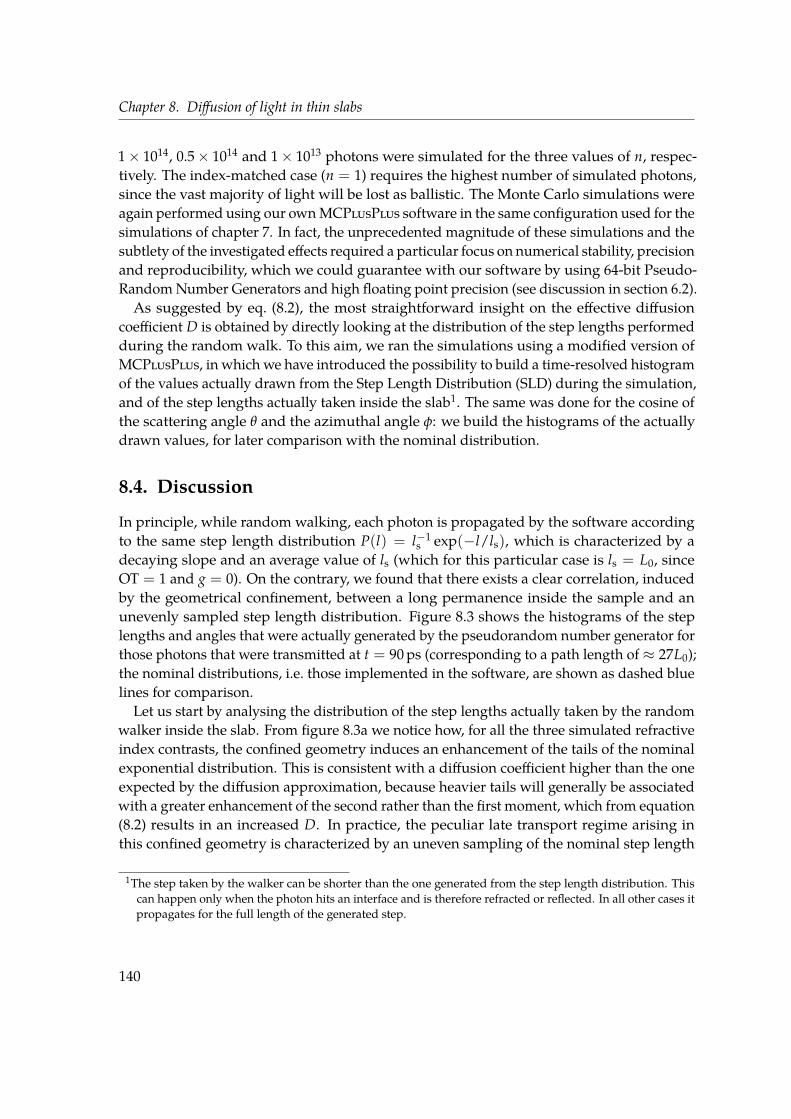
Chapter 8. Diffusion of light in thin slabs
1× 10¹⁴, 0.5× 10¹⁴ and 1× 10¹³ photons were simulated for the three values of n, respec-tively. The index-matched case (n = 1) requires the highest number of simulated photons,since the vast majority of light will be lost as ballistic. The Monte Carlo simulations wereagain performed using our ownMCPlusPlus software in the same configuration used for thesimulations of chapter 7. In fact, the unprecedented magnitude of these simulations and thesubtlety of the investigated effects required a particular focus on numerical stability, precisionand reproducibility, which we could guarantee with our software by using 64-bit Pseudo-RandomNumber Generators and high floating point precision (see discussion in section 6.2).As suggested by eq. (8.2), the most straightforward insight on the effective diffusion
coefficient D is obtained by directly looking at the distribution of the step lengths performedduring the random walk. To this aim, we ran the simulations using a modified version ofMCPlusPlus, in which we have introduced the possibility to build a time-resolved histogramof the values actually drawn from the Step Length Distribution (SLD) during the simulation,and of the step lengths actually taken inside the slab1. The same was done for the cosine ofthe scattering angle θ and the azimuthal angle φ: we build the histograms of the actuallydrawn values, for later comparison with the nominal distribution.
8.4. Discussion
In principle, while random walking, each photon is propagated by the software accordingto the same step length distribution P(l) = l−1
s exp(−l/ls), which is characterized by adecaying slope and an average value of ls (which for this particular case is ls = L0, sinceOT = 1 and g = 0). On the contrary, we found that there exists a clear correlation, inducedby the geometrical confinement, between a long permanence inside the sample and anunevenly sampled step length distribution. Figure 8.3 shows the histograms of the steplengths and angles that were actually generated by the pseudorandom number generator forthose photons that were transmitted at t = 90 ps (corresponding to a path length of ≈ 27L0);the nominal distributions, i.e. those implemented in the software, are shown as dashed bluelines for comparison.
Let us start by analysing the distribution of the step lengths actually taken by the randomwalker inside the slab. From figure 8.3a we notice how, for all the three simulated refractiveindex contrasts, the confined geometry induces an enhancement of the tails of the nominalexponential distribution. This is consistent with a diffusion coefficient higher than the oneexpected by the diffusion approximation, because heavier tails will generally be associatedwith a greater enhancement of the second rather than the first moment, which from equation(8.2) results in an increased D. In practice, the peculiar late transport regime arising inthis confined geometry is characterized by an uneven sampling of the nominal step length
1The step taken by the walker can be shorter than the one generated from the step length distribution. Thiscan happen only when the photon hits an interface and is therefore refracted or reflected. In all other cases itpropagates for the full length of the generated step.
140
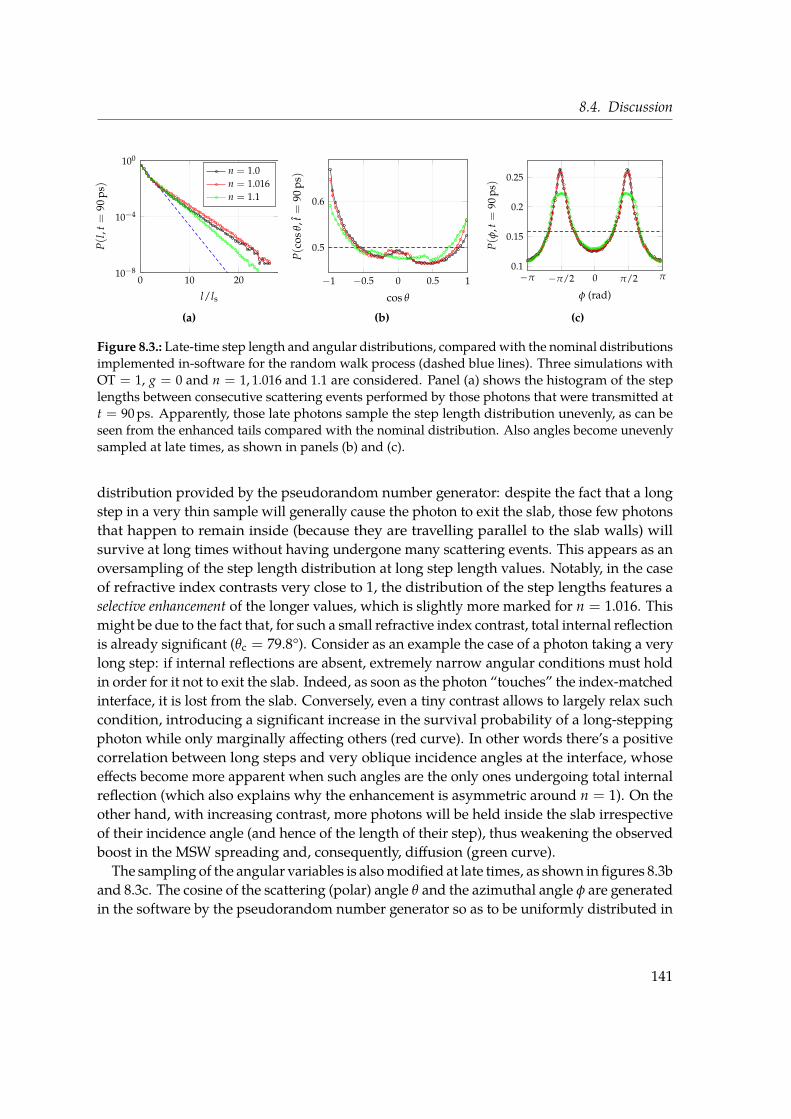
8.4. Discussion
0 10 2010−8
10−4
100
l/ls
P(l
,t=
90ps)
n = 1.0n = 1.016n = 1.1
(a)
−1 −0.5 0 0.5 1
0.5
0.6
cos θP(c
osθ,
t=
90ps)
(b)
−π −π/2 0 π/2 π0.1
0.15
0.2
0.25
φ (rad)
P(φ
,t=
90ps)
(c)
Figure 8.3.: Late-time step length and angular distributions, comparedwith the nominal distributionsimplemented in-software for the random walk process (dashed blue lines). Three simulations withOT = 1, g = 0 and n = 1, 1.016 and 1.1 are considered. Panel (a) shows the histogram of the steplengths between consecutive scattering events performed by those photons that were transmitted att = 90 ps. Apparently, those late photons sample the step length distribution unevenly, as can beseen from the enhanced tails compared with the nominal distribution. Also angles become unevenlysampled at late times, as shown in panels (b) and (c).
distribution provided by the pseudorandom number generator: despite the fact that a longstep in a very thin sample will generally cause the photon to exit the slab, those few photonsthat happen to remain inside (because they are travelling parallel to the slab walls) willsurvive at long times without having undergone many scattering events. This appears as anoversampling of the step length distribution at long step length values. Notably, in the caseof refractive index contrasts very close to 1, the distribution of the step lengths features aselective enhancement of the longer values, which is slightly more marked for n = 1.016. Thismight be due to the fact that, for such a small refractive index contrast, total internal reflectionis already significant (θc = 79.8°). Consider as an example the case of a photon taking a verylong step: if internal reflections are absent, extremely narrow angular conditions must holdin order for it not to exit the slab. Indeed, as soon as the photon “touches” the index-matchedinterface, it is lost from the slab. Conversely, even a tiny contrast allows to largely relax suchcondition, introducing a significant increase in the survival probability of a long-steppingphoton while only marginally affecting others (red curve). In other words there’s a positivecorrelation between long steps and very oblique incidence angles at the interface, whoseeffects become more apparent when such angles are the only ones undergoing total internalreflection (which also explains why the enhancement is asymmetric around n = 1). On theother hand, with increasing contrast, more photons will be held inside the slab irrespectiveof their incidence angle (and hence of the length of their step), thus weakening the observedboost in the MSW spreading and, consequently, diffusion (green curve).
The sampling of the angular variables is alsomodified at late times, as shown in figures 8.3band 8.3c. The cosine of the scattering (polar) angle θ and the azimuthal angle φ are generatedin the software by the pseudorandom number generator so as to be uniformly distributed in
141
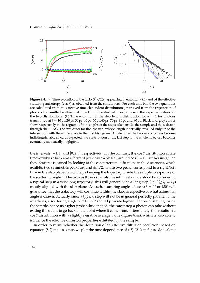
Chapter 8. Diffusion of light in thin slabs
0 10 20−0.1
0
0.1
0.2
0.3
t/τ
〈cos
θ〉
0.5
1
1.5
〈l2 〉/
2〈l〉
(mm
)
(a)
0 10 20
10−7
10−5
10−3
10−1
l/ls
P(l
,t)
(b)
Figure 8.4.: (a) Time evolution of the ratio 〈l2〉/2〈l〉 appearing in equation (8.2) and of the effectivescattering anisotropy 〈cos θ〉 as obtained from the simulations. For each time bin, the two quantitiesare calculated from the effective time-dependent distributions, retrieved from the trajectories ofphotons transmitted within that time bin. Blue dashed lines represent the expected values forthe two distributions. (b) Time evolution of the step length distribution for n = 1 for photonstransmitted at t = 10 ps, 20 ps, 30 ps, 40 ps, 50 ps, 60 ps, 70 ps, 80 ps and 90 ps. Black and grey curvesshow respectively the histograms of the lengths of the steps taken inside the sample and those drawnthrough the PRNG. The two differ for the last step, whose length is actually travelled only up to theintersection with the exit surface in the first histogram. At late times the two sets of curves becomeindistinguishable since, as expected, the contribution of the last step to the whole trajectory becomeseventually statistically negligible.
the intervals [−1, 1] and [0, 2π), respectively. On the contrary, the cos θ distribution at latetimes exhibits a back and a forward peak, with a plateau around cos θ = 0. Further insight onthese features is gained by looking at the concurrent modifications in the φ statistics, whichexhibits two symmetric peaks around ±π/2. These two peaks correspond to a right/leftturn in the slab plane, which helps keeping the trajectory inside the sample irrespective ofthe scattering angle θ. The two cos θ peaks can also be intuitively understood by consideringa typical step in a very long trajectory: this will generally be a long step (i.e. l & ls = L0)mostly aligned with the slab plane. As such, scattering angles close to θ = 0° or 180° willguarantee that the trajectory will continue within the slab, irrespective of what azimuthalangle is drawn. Actually, since a typical step will not be in general perfectly parallel to theinterfaces, a scattering angle of θ ≈ 180° should provide higher chances of staying insidethe sample, hence its higher probability: indeed, the safest step a photon can take withoutexiting the slab is to go back to the point where it came from. Interestingly, this results in acos θ distribution with a slightly negative average value (figure 8.4a), which is also able toinfluence the effective diffusion properties exhibited by the sample.In order to verify whether the definition of an effective diffusion coefficient based on
equation (8.2) makes sense, we plot the time dependence of 〈l2〉/2〈l〉 in figure 8.4a, along
142
8.5. Conclusions
with its nominal value of 1 plotted as a dashed blue line. Each point is computed startingfrom the empirical distributions registered for those photons that were transmitted withinthat time bin. The obtained curves successfully validate our interpretation based on arandomwalk picture of the diffusive process as expressed by equation (8.2), exhibiting goodqualitative agreement with the behaviour for D obtained from the mean square width slope.Indeed, the red curve (n = 1.016) features an enhanced 〈l2〉/2〈l〉 ratio. In principle, theoverall observed diffusion process will be influenced by both the modified step length andangular distributions, which in the investigated configurations appear to have oppositeeffects. While the latter would indeed tend to slightly slow down diffusion (〈cos θ〉 < 0), thepredominant effect clearly originates from the step lengths being substantially increased,leading to the observed enhanced in-plane diffusion especially for n = 1.016. Differentconfigurations might lead to a different overall balance between these two effects, whichalso appear to saturate to their respective asymptotic values on slightly different time scales,further illustrating the need for additional investigation even for the simple homogeneousand isotropic single slab model.
The asymptotic nature of the observed distributions suggests that a well-defined diffusioncoefficient does still exist, albeit not the one given by the diffusion approximation. This isfurther illustrated in figure 8.4b, where the time evolution of the step length distribution isshown for n = 1 (black curves; the n = 1.016 and 1.1 cases are analogous). The time-resolveddistributions seem to converge towards a single asymptotic envelope distribution with awell defined asymptotic decay which seems to be uniquely determined by the propertiesof the sample. It is interesting to compare the histogram of the actual steps performedinside the sample (black curves) with the histogram of the ones drawn from the PRNG(grey curves). The two differ only for the last step, whose length is respectively consideredeither partially (up to the intersection with the interface) or totally. Interestingly, once theasymptotic diffusive regime is reached, the sample appears to be less scattering than itactually is. Indeed, photons migrate as if the scatterers were further apart than they reallyare, i.e. with an effective transport mean free path which is greater than the one intrinsic tothe material. It should be noted that such discrepancy — which we are now able to correctlyidentify as the emerging of an effective transverse diffusion coefficient — has already beenreported experimentally in samples with an optical thickness as high as 8 [47], suggestingthat it can indeed represent an appreciable issue in a broad range of applications.
8.5. Conclusions
We have studied light transport in optically thin samples and shown that, at late times, adiffusive regime corresponding to in-plane transport sets in, exhibiting peculiar featuresespecially for small refractive index contrasts. Indeed, we were able to follow the evolutionof light deeply into the multiple-scattering regime, where light is undoubtedly diffusing asthe radial intensity profiles and their linear variance expansion clearly demonstrate.
143

Chapter 8. Diffusion of light in thin slabs
The unprecedented scale of the Monte Carlo simulations that we performed allows us toinspect transport properties on exceptionally long time scales. A subtle interplay occurringbetween the actual thickness of the slab, the refractive index contrast and the scatteringanisotropy emerges from our data. This results in a regime that is properly diffusive butwhich cannot be described in terms of the standard diffusion approximation. Such interplaygives rise to a different diffusion coefficient which emerges naturally from the overall opticaland geometric boundary conditions of the sample, and is uniquely determined by themthrough yet unknown relations. Following the usual approach based on the diffusionapproximation, it may be argued that it could be possible to take into account all the observedeffects by means of some refined extrapolated boundary condition. On the contrary, theoptical thickness must be regarded as one of the parameters actively and independentlyaffecting transport properties.Our results show that the currently established theoretical framework linking radiative
transfer theory to diffusion needs to be further refined, especially for thin systems and moregenerally for confined geometries. In particular, concerning microscopic optical propertiessuch as the scattering anisotropy or the mean free path, it seems appropriate to introduce adistinction between an intrinsic and an effective counterpart, where the former is the one thatwe are typically interested in retrieving while the latter might have a very different value andnature (e.g. tensorial instead of scalar) depending on incidental geometric conditions. Wehave shown in fact that a homogeneous, isotropic slice of a certain disordered material willeventually reach an asymptotic, multiple-scattering regime characterized by different (andpossibly anisotropic) statistical distributions, depending on both sample size and boundaryconditions.It is worth stressing that only a small fraction of incoming light is actually subject to
this effective transport mean free path. Indeed, in optically thin systems the vast major-ity of transmitted light is ballistic, therefore only a few photons will reach the asymptoticmultiple-scattering regime. Nonetheless experimental techniques capable of detecting thisdiscrepancy are nowadays available [47]. Furthermore, other applications can be envi-sioned where multiple-scattering in thin layers, even if limited to few photons, could play asignificant role (e.g. random lasers).
Finally, despite our case study is in the field of light transport, randomwalks are extremelygeneral models for a broad range of phenomena in complex systems, frommolecular kineticsto social behaviours. Therefore our findings could apply also to other scenarios where tightgeometric confinement holds and analogous boundary conditions can be modelled. Inthis respect we demonstrated how, depending on the application, the interplay betweentransport properties and the environment geometry can give rise to sharp and unexpectedmacroscopic migration features, which can be possibly exploited as an engineering degreeof freedom to enhance transport.
144

References
[1] C. Mencuccini and V. Silvestrini. Fisica 2. Elettromagnetismo-ottica. Corso di fisica per lefacoltà scientifiche. Con esempi ed esercizi. Liguori, 1998.
[2] J. Jackson. Classical Electrodynamics. Wiley, 1998.[3] E. Akkermans and G. Montambaux. Mesoscopic physics of electrons and photons. Cam-
bridge University Press, 2007.[4] H. van de Hulst. Light Scattering by Small Particles. Dover Books on Physics. Dover
Publications, 2012.[5] E. Alerstam. “Optical spectroscopy of turbid media: time-domain measurements and
accelerated Monte Carlo modelling”. PhD thesis. Lund University, 2011.[6] M. I. Mishchenko. “Maxwell’s equations, radiative transfer, and coherent backscat-
tering: A general perspective”. In: Journal of Quantitative Spectroscopy and RadiativeTransfer 101, 3 (2006), pp. 540–555.
[7] M. Mishchenko, L. Travis, and A. Lacis.Multiple Scattering of Light by Particles: Radia-tive Transfer and Coherent Backscattering. Cambridge University Press, 2006.
[8] L. Wang and H. Wu. Biomedical Optics: Principles and Imaging. Wiley, 2007.[9] M. I. Mishchenko. “Vector radiative transfer equation for arbitrarily shaped and
arbitrarily oriented particles: a microphysical derivation from statistical electromag-netics”. In: Applied Optics 41, 33 (2002), pp. 7114–7134.
[10] S. Chandrasekhar. Radiative Transfer. Dover, 1960.[11] D. Contini, F. Martelli, and G. Zaccanti. “Photon migration through a turbid slab
described by amodel based on diffusion approximation. I. Theory”. In:Applied Optics36, 19 (1997), pp. 4587–4599.
[12] A. Ishimaru.Wave propagation and scattering in random media. Elsevier Science, 2013.[13] R. C. Haskell, L. O. Svaasand, T.-T. Tsay, T.-C. Feng, B. J. Tromberg, and M. S. McA-
dams. “Boundary conditions for the diffusion equation in radiative transfer”. In:JOSA A 11, 10 (1994), pp. 2727–2741.
[14] D. Durian. “Influence of boundary reflection and refraction on diffusive photontransport”. In: Phys. Rev. E 50, 2 (1994), p. 857.
[15] J. Zhu, D. Pine, and D. Weitz. “Internal reflection of diffusive light in randommedia”.In: Phys. Rev. A 44, 6 (1991), p. 3948.
145

References
[16] M. Keijzer, W. M. Star, and P. R. Storchi. “Optical diffusion in layered media”. In:Applied Optics 27, 9 (1988), pp. 1820–1824.
[17] M. S. Patterson, B. Chance, and B. C. Wilson. “Time resolved reflectance and trans-mittance for the noninvasive measurement of tissue optical properties”. In: AppliedOptics 28, 12 (1989), pp. 2331–2336.
[18] P. Barthelemy. “Anomalous Transport of Light”. PhD thesis. European Laboratoryof Nonlinear Spectroscopy (LENS), 2009.
[19] L. Pattelli. “Ultrafast time- and space-resolved investigation of diffused light trans-mission through strongly heterogeneous media”. MS Thesis. European Laboratoryof Nonlinear Spectroscopy (LENS), 2013.
[20] T. J. Huisman. “Faster than diffusive light. Temporal behavior of superdiffusive light”.Internship Thesis. University of Twente and LENS, 2011.
[21] D. S. Wiersma, P. Bartolini, A. Lagendijk, and R. Righini. “Localization of light in adisordered medium”. In: Nature 390, 6661 (1997), pp. 671–673.
[22] T. Svensson, R. Savo, E. Alerstam, K. Vynck, M. Burresi, and D. S. Wiersma. “Exploit-ing breakdown of the similarity relation for diffuse light transport: simultaneousretrieval of scattering anisotropy and diffusion constant”. In:Optics Letters 38, 4 (2013),pp. 437–439.
[23] M. I. Mishchenko. “Gustav Mie and the fundamental concept of electromagneticscattering by particles: a perspective”. In: Journal of Quantitative Spectroscopy andRadiative Transfer 110, 14 (2009), pp. 1210–1222.
[24] C. Rycroft and M. Bazant. “Lecture 1: Introduction to Random Walks and Diffusion”.In: Lecture Notes on Random Walks and Diffusion, Department of Mathematics-MIT 2(2005).
[25] L. Wang, S. L. Jacques, and L. Zheng. “MCML—Monte Carlo modeling of lighttransport in multi-layered tissues”. In: Computer methods and programs in biomedicine47, 2 (1995), pp. 131–146.
[26] E. Alerstam, T. Svensson, and S.Andersson-Engels. “Parallel computingwith graphicsprocessing units for high-speed Monte Carlo simulation of photon migration”. In:Journal of Biomedical Optics 13, 6 (2008), pp. 060504–060504.
[27] G. Mazzamuto and L. Pattelli.MCPlusPlus: a Monte Carlo C++ code for radiative trans-port.url: http://www.lens.unifi.it/quantum-nanophotonics/mcplusplus/
[28] A. Doronin and I. Meglinski. “Online object orientedMonte Carlo computational toolfor the needs of biomedical optics”. In: Biomedical optics express 2, 9 (2011), p. 2461.
[29] M. H. Kalos and P. A. Whitlock.Monte Carlo methods. John Wiley & Sons, 2008.
146

References
[30] P. Milsom. “A ray-optic, Monte Carlo, description of a Gaussian beam waist–appliedto reverse saturable absorption”. In: Applied Physics B 70, 4 (2000), pp. 593–599.
[31] L. G. Henyey and J. L. Greenstein. “Diffuse radiation in the galaxy”. In: The Astro-physical Journal 93 (1941), pp. 70–83.
[32] G. Mazzamuto, L. Pattelli, D. Wiersma, and C. Toninelli.Deducing effective light trans-port parameters in optically thin systems. Sept. 2015.arXiv: 1509.04027 [physics.optics]. Accepted for publication in NJP.
[33] M. Burresi, L. Cortese, L. Pattelli, M. Kolle, P. Vukusic, D. S. Wiersma, U. Steiner, andS. Vignolini. “Bright-white beetle scales optimise multiple scattering of light”. In:Scientific Reports 4, 6075 (2014).
[34] G. Zonios, J. Bykowski, and N. Kollias. “Skin melanin, hemoglobin, and light scat-tering properties can be quantitatively assessed in vivo using diffuse reflectancespectroscopy”. In: Journal of Investigative Dermatology 117, 6 (2001), pp. 1452–1457.
[35] J. R. Mourant, J. P. Freyer, A. H. Hielscher, A. A. Eick, D. Shen, and T. M. Johnson.“Mechanisms of light scattering from biological cells relevant to noninvasive optical-tissue diagnostics”. In: Applied Optics 37, 16 (1998), pp. 3586–3593.
[36] M. Hammer, A. Roggan, D. Schweitzer, and G. Muller. “Optical properties of ocularfundus tissues-an in vitro study using the double-integrating-sphere technique andinverseMonte Carlo simulation”. In: Physics inMedicine and biology 40, 6 (1995), p. 963.
[37] E. K. Chan, B. Sorg, D. Protsenko, M. O’Neil, M. Motamedi, and A. J. Welch. “Ef-fects of compression on soft tissue optical properties”. In: Selected Topics in QuantumElectronics, IEEE Journal of 2, 4 (1996), pp. 943–950.
[38] V. Backman, R. Gurjar, K. Badizadegan, I. Itzkan, R. R. Dasari, L. T. Perelman, andM. Feld. “Polarized light scattering spectroscopy for quantitative measurement ofepithelial cellular structures in situ”. In: Selected Topics in Quantum Electronics, IEEEJournal of 5, 4 (1999), pp. 1019–1026.
[39] Y. Du, X. Hu,M. Cariveau, X. Ma, G. Kalmus, and J. Lu. “Optical properties of porcineskin dermis between 900 nm and 1500 nm”. In: Physics in Medicine and biology 46, 1(2001), p. 167.
[40] N. Ugryumova, S. J. Matcher, and D. P. Attenburrow. “Measurement of bone mineraldensity via light scattering”. In: Physics in Medicine and biology 49, 3 (2004), p. 469.
[41] C. L. Darling, G. D. Huynh, and D. Fried. “Light scattering properties of natural andartificially demineralized dental enamel at 1310 nm”. In: Journal of Biomedical Optics11, 3 (2006), pp. 034023–034023.
[42] A. Liemert and A. Kienle. “Exact and efficient solution of the radiative transportequation for the semi-infinite medium”. In: Scientific Reports 3, 2018 (2013).
147
References
[43] A. Liemert and A. Kienle. “Analytical solutions of the simplified spherical harmonicsequations”. In: Optics Letters 35, 20 (2010), pp. 3507–3509.
[44] R. Elaloufi, R. Carminati, and J.-J. Greffet. “Time-dependent transport through scat-tering media: from radiative transfer to diffusion”. In: Journal of Optics A: Pure andApplied Optics 4, 5 (2002), S103.
[45] A. Garofalakis, G. Zacharakis, G. Filippidis, E. Sanidas, D. D. Tsiftsis, V. Ntziachristos,T. G. Papazoglou, and J. Ripoll. “Characterization of the reduced scattering coefficientfor optically thin samples: theory and experiments”. In: Journal of Optics A: Pure andApplied Optics 6, 7 (2004), p. 725.
[46] V. Venugopalan, J. You, and B. Tromberg. “Radiative transport in the diffusion ap-proximation: an extension for highly absorbing media and small source-detectorseparations”. In: Phys. Rev. E 58, 2 (1998), p. 2395.
[47] L. Pattelli, R. Savo, M. Burresi, and D. Wiersma. Spatio-temporal visualization of lighttransport in complex photonic structures. Sept. 2015.arXiv: 1509.05735 [physics.optics]
[48] K. Yoo, F. Liu, and R. Alfano. “When does the diffusion approximation fail to describephoton transport in random media?” In: Phys. Rev. Lett. 64, 22 (1990), p. 2647.
[49] E. Alerstam, S. Andersson-Engels, and T. Svensson. “Improved accuracy in time-resolved diffuse reflectance spectroscopy”. In: Optics Express 16, 14 (2008), pp. 10440–10454.
[50] R. Elaloufi, R. Carminati, and J.-J. Greffet. “Diffusive-to-ballistic transition in dynamiclight transmission through thin scattering slabs: a radiative transfer approach”. In:JOSA A 21, 8 (2004), pp. 1430–1437.
[51] F. P. Bolin, L. E. Preuss, R. C. Taylor, and R. J. Ference. “Refractive index of somemammalian tissues using a fiber optic cladding method”. In: Applied Optics 28, 12(1989), pp. 2297–2303.
[52] A. Pifferi, P. Taroni, G. Valentini, and S. Andersson-Engels. “Real-time method forfitting time-resolved reflectance and transmittancemeasurements with aMonte Carlomodel”. In: Applied Optics 37, 13 (1998), pp. 2774–2780.
[53] J. S. Dam, T. Dalgaard, P. E. Fabricius, and S. Andersson-Engels. “Multiple polyno-mial regression method for determination of biomedical optical properties fromintegrating sphere measurements”. In: Applied Optics 39, 7 (2000), pp. 1202–1209.
[54] N. Rajaram, T. H. Nguyen, and J. W. Tunnell. “Lookup table–based inverse model fordetermining optical properties of turbid media”. In: Journal of Biomedical Optics 13, 5(2008), pp. 050501–050501.
148

References
[55] R. Hennessy, S. L. Lim, M. K. Markey, and J. W. Tunnell. “Monte Carlo lookuptable-based inverse model for extracting optical properties from tissue-simulatingphantoms using diffuse reflectance spectroscopy”. In: Journal of Biomedical Optics 18,3 (2013), pp. 037003–037003.
[56] J. Müller, B. Rech, J. Springer, and M. Vanecek. “TCO and light trapping in siliconthin film solar cells”. In: Solar Energy 77, 6 (2004), pp. 917–930.
[57] W. Beyer, J. Hüpkes, and H. Stiebig. “Transparent conducting oxide films for thinfilm silicon photovoltaics”. In: Thin Solid Films 516, 2 (2007), pp. 147–154.
[58] F. Huang, D. Chen, X. L. Zhang, R. A. Caruso, and Y.-B. Cheng. “Dual-FunctionScattering Layer of Submicrometer-SizedMesoporous TiO2 Beads for High-EfficiencyDye-Sensitized Solar Cells”. In: Advanced Functional Materials 20, 8 (2010), pp. 1301–1305.
[59] G. Yang, J. Zhang, P. Wang, Q. Sun, J. Zheng, and Y. Zhu. “Light scattering en-hanced photoanodes for dye-sensitized solar cells prepared by carbon spheres/TiO2 nanoparticle composites”. In: Current Applied Physics 11, 3 (2011), pp. 376–381.
[60] F. E. Gálvez, E. Kemppainen, H. Míguez, and J. Halme. “Effect of diffuse light scat-tering designs on the efficiency of dye solar cells: an integral optical and electricaldescription”. In: The Journal of Physical Chemistry C 116, 21 (2012), pp. 11426–11433.
[61] X. Zhang and Z.-Q. Zhang. “Wave transport through thin slabs of random mediawith internal reflection: Ballistic to diffusive transition”. In: Phys. Rev. E 66, 1 (2002),p. 016612.
[62] J. B. Fishkin, S. Fantini, E. Gratton, et al. “Gigahertz photon density waves in a turbidmedium: theory and experiments”. In: Phys. Rev. E 53, 3 (1996), p. 2307.
[63] F. Martelli, M. Bassani, L. Alianelli, L. Zangheri, and G. Zaccanti. “Accuracy ofthe diffusion equation to describe photon migration through an infinite medium:numerical and experimental investigation”. In: Physics in Medicine and biology 45, 5(2000), p. 1359.
[64] V. Ntziachristos and B. Chance. “Accuracy limits in the determination of absoluteoptical properties using time-resolved NIR spectroscopy”. In: Medical physics 28, 6(2001), pp. 1115–1124.
[65] F. Scheffold, R. Lenke, R. Tweer, and G. Maret. “Localization or classical diffusion oflight?” In: Nature 398, 6724 (1999), pp. 206–207.
[66] D. S. Wiersma, J. G. Rivas, P. Bartolini, A. Lagendijk, and R. Righini. “Reply: Local-ization or classical diffusion of light?” In: Nature 398 (1999), p. 207.
[67] H. Hu, A. Strybulevych, J. H. Page, S. E. Skipetrov, and B. A. van Tiggelen. “Localiza-tion of ultrasound in a three-dimensional elastic network”. In: Nature Physics 4, 12(2008), pp. 945–948.
149

References
[68] N. Cherroret, S. Skipetrov, and B. Van Tiggelen. “Transverse confinement of wavesin three-dimensional random media”. In: Phys. Rev. E 82, 5 (2010), p. 056603.
[69] T. Sperling, W. Buehrer, C. M. Aegerter, and G. Maret. “Direct determination of thetransition to localization of light in three dimensions”. In:Nature Photonics 7, 1 (2012),pp. 48–52.
[70] F. MacKintosh and S. John. “Diffusing-wave spectroscopy and multiple scattering oflight in correlated random media”. In: Phys. Rev. B 40, 4 (1989), p. 2383.
[71] K. Yoo and R. Alfano. “Time-resolved coherent and incoherent components of for-ward light scattering in random media”. In: Optics Letters 15, 6 (1990), pp. 320–322.
[72] J.-P. Bouchard, I. Veilleux, R. Jedidi, I. Noiseux, M. Fortin, and O. Mermut. “Referenceoptical phantoms for diffuse optical spectroscopy. Part 1–Error analysis of a timeresolved transmittance characterization method”. In: Optics Express 18, 11 (2010),pp. 11495–11507.
[73] L. Spinelli, F. Martelli, A. Farina, A. Pifferi, A. Torricelli, R. Cubeddu, and G. Zaccanti.“Calibration of scattering and absorption properties of a liquid diffusive medium atNIR wavelengths. Time-resolved method”. In: Optics Express 15, 11 (2007), pp. 6589–6604.
[74] L. Pattelli, R. Savo, M. Burresi, and D. Wiersma. Spatio-temporal visualization of lighttransport in complex photonic structures. Submitted to Light: Science & Applications.2015.arXiv: 1509.05735 [physics.optics]
[75] R. Graaff,M. Koelink, F. DeMul,W. Zijistra, A. Dassel, and J. Aarnoudse. “CondensedMonte Carlo simulations for the description of light transport”. In: Applied Optics 32,4 (1993), pp. 426–434.
[76] A. Kienle and M. S. Patterson. “Determination of the optical properties of turbidmedia from a single Monte Carlo simulation”. In: Physics in Medicine and biology 41,10 (1996), p. 2221.
[77] H. Xu, T. J. Farrell, and M. S. Patterson. “Investigation of light propagation models todetermine the optical properties of tissue from interstitial frequency domain fluencemeasurements”. In: Journal of Biomedical Optics 11, 4 (2006), pp. 041104–041104.
[78] E. Alerstam, S. Andersson-Engels, and T. Svensson. “White Monte Carlo for time-resolved photon migration”. In: Journal of Biomedical Optics 13, 4 (2008), pp. 041304–041304.
[79] M. Martinelli, A. Gardner, D. Cuccia, C. Hayakawa, J. Spanier, and V. Venugopalan.“Analysis of single Monte Carlo methods for prediction of reflectance from turbidmedia”. In: Optics Express 19, 20 (2011), pp. 19627–19642.
150
References
[80] A. M. Nilsson, R. Berg, and S. Andersson-Engels. “Measurements of the opticalproperties of tissue in conjunction with photodynamic therapy”. In: Applied Optics34, 21 (1995), pp. 4609–4619.
[81] A. Roggan, H. J. Albrecht, K. Doerschel, O. Minet, and G. J. Mueller. “Experimentalset-up and Monte-Carlo model for the determination of optical tissue propertiesin the wavelength range 330 to 1100 nm”. In: International Symposium on BiomedicalOptics Europe’94. International Society for Optics and Photonics. 1995, pp. 21–36.
[82] P. Thueler, I. Charvet, F. Bevilacqua, M. S. Ghislain, G. Ory, P. Marquet, P. Meda,B. Vermeulen, and C. Depeursinge. “In vivo endoscopic tissue diagnostics based onspectroscopic absorption, scattering, and phase function properties”. In: Journal ofBiomedical Optics 8, 3 (2003), pp. 495–503.
[83] J. S. Dam, N. Yavari, S. Sørensen, and S. Andersson-Engels. “Real-time absorption andscattering characterization of slab-shaped turbid samples obtained by a combinationof angular and spatially resolved measurements”. In: Applied Optics 44, 20 (2005),pp. 4281–4290.
[84] G. M. Palmer and N. Ramanujam. “Monte Carlo-based inverse model for calculatingtissue optical properties. Part I: Theory and validation on synthetic phantoms”. In:Applied Optics 45, 5 (2006), pp. 1062–1071.
[85] H. Karlsson, I. Fredriksson, M. Larsson, and T. Strömberg. “Inverse Monte Carlofor estimation of scattering and absorption in liquid optical phantoms”. In: OpticsExpress 20, 11 (2012), pp. 12233–12246.
[86] M. Mangel and F. J. Samaniego. “AbrahamWald’s work on aircraft survivability”. In:Journal of the American Statistical Association 79, 386 (1984), pp. 259–267.
[87] “A reprint of “A method of estimating plane vulnerability based on damage ofsurvivors” by AbrahamWald”. In: CRC (432 1980).
[88] M. Leonetti and C. López. “Measurement of transport mean-free path of light in thinsystems”. In: Optics Letters 36, 15 (2011), pp. 2824–2826.
[89] T. Svensson, K. Vynck, M. Grisi, R. Savo, M. Burresi, and D. S. Wiersma. “Holeyrandom walks: Optics of heterogeneous turbid composites”. In: Phys. Rev. E 87, 2(2013), p. 022120.
[90] E. Alerstam. “Anisotropic diffusive transport: Connecting microscopic scatteringand macroscopic transport properties”. In: Phys. Rev. E 89 (6 2014), p. 063202.
151


Part III.
Attachments


Necklace state hallmark in disordered 2D photonic systems
Fabrizio Sgrignuoli,1, 2 Giacomo Mazzamuto,2, 3 Niccolo Caselli,1, 3 Francesca Intonti,1, 3
Francesco Saverio Cataliotti,1, 3, 4 Massimo Gurioli,1, 3 and Costanza Toninelli2, 3, 4
1Dipartimento di Fisica ed Astronomia, Universita di Firenze,Via Sansone 1, I-50019 Sesto F.no, Firenze, Italy
2CNR-INO, Istituto Nazionale di Ottica, Via Carrara 1, 50019 Sesto F.no, Firenze, Italy∗3LENS and Universita di Firenze, Via Carrara 1, 50019 Sesto F.no, Firenze, Italy
4QSTAR, Largo Fermi 2, I-50125 Firenze, Italy
Necklace states arise from the coupling of otherwise confined modes in disordered photonic systemsand open high transmission channels in strongly scattering media. Despite their potential relevancein the transport properties of photonic systems, necklace-state statistical occurrence in dimensionshigher than one is hard to measure, because of the lack of a decisive signature. In this work we providean efficient prescription to tell apart in a single measurement a coupled-mode from a single localizedstate in a complex scattering problem, exploiting the analogy with well-characterized coupled cavitiesin photonic crystals. The phase spatial distribution of the electromagnetic field has been numericallycalculated and analyzed as a function of the coupling strength and of detuning between interactingmodes, respectively for coupled photonic crystal cavities and for partially disordered systems. Resultsconsistently show that when localized modes spectrally and spatially overlap only over a small surfaceextent, synchronous oscillation does not build up and the phase spatial distribution splits in twodistinct peaks. Having established such bimodal distribution as a necklace hallmark, this paperopens the possibility to assess and eventually tailor the role of necklace states in random systems,e.g. by varying correlations.
Reprinted with permission from F. Sgrignuoli, G. Mazzamuto, N. Caselli, F. Intonti, F. S. Cataliotti, M.
Gurioli, and C. Toninelli. Necklace state hallmark in disordered 2D photonic systems. In: ACS Photonics 2,
11 (2015), pp. 1636–1643. © 2015 American Chemical Society.
Transport properties in complex systems depend criti-cally on the interplay between disorder, correlations andinteraction. Communication, i.e. transport of informa-tion through physical carriers, is described in the sameparameter space. Photons are ideal candidates for thispurpose, both for fundamental and practical reasons. In-deed, they are inherently characterized by a negligibleinteraction cross section and well-established technologies,from self assembly to the most complex lithographic pro-cesses, enable efficient manipulation of the light flow inartificial photonic structures [1].
Photonic crystal fibers are perhaps the first exampleof a commercial product along this line. Fabrication im-perfections however induce unwanted scattering and hin-der performances, typically determining an upper boundto the propagation length in one-dimensional photonicwaveguides [2, 3]. However, scattering of light should
not be regarded as a simple linear loss channel. As thor-oughly discussed in Ref. [4], propagation is inhibited asthe sample length exceeds a critical length scale, dubbedlocalization length, because of the forming of trap statestrough interference. This phenomenology is related to thehalt of diffusion determined by the localization of the elec-tronic wave-function in certain semiconductors [5]. Suchapparently detrimental factor has been exploited, e.g bySapienza and co-workers, to modify the optical propertiesof solid-state quantum emitters coupled to confined opti-cal modes in 1D disordered systems [6], suggesting thatAnderson localized modes might offer an unconventionalplatform for cavity quantum electrodynamics applications.As a matter of fact, the progress in optical communica-tions relies on the understanding of transport mechanismsin presence of disorder.
Consider, as an example, the case of light control ona chip, in two dimensional photonic crystal structures,affected by random imperfections. Due to the strongdispersion in the density of states, disorder induces theformation of localized modes preferentially at the band-edge [7]. The transport properties are strongly relatedto the nature of such states. Indeed, in the language ofeigenchannel statistics, localization corresponds to thesingle-channel regime [8], where every transmission chan-nel is univocally related to the formation of a quasi-modein the structure [9]. Interestingly, these states can be ei-ther single localized ones, featuring exponentially decayingtails, or multi-peaked states, formed by the hybridizationof two or more separate modes. Besides robust confine-
155

ment hence, the complexity of light transport allowingfor high transmission channels generally impacts the con-nectivity between distant points, defined as the numberof eigenchannels connecting them [10].
The occurrence of so-called necklace states has beenoriginally predicted by Pendry [11], then observed intime-resolved experiments [12] and by measuring cumu-lative phase lag of the transmitted light field [13] in one-dimensional systems. In 2D however, where the outputin transmission is a complex speckle pattern, phase lagin not easily defined and a different approach is requiredto single out coupled modes. Such states in 2D disor-dered structures have been experimentally induced andmonitored by means of a local control of the refractiveindex, which gradually varied the coupling strength [14].However, the probability of their natural occurrence isnot yet known, especially because of the lack of a decisivesignature, enabling a statistical study over ensembles ofrealizations. Information about spectra, even if spatiallyresolved, is indeed not sufficient for this purpose, sincetwo modes which are accidentally resonant cannot bediscriminated from a single more extended mode. In Ref[15], the phase spatial probability distribution has beensuggested as a key to the problem, although remaining asingle case-study.
Here we present an extensive numerical analysis anddata interpretation for the connectivity of an integratedoptical system, where scattering occurs in 2D photoniccrystals with a small amount of disorder. In particular, wedefine and test an indicator, which combines the near-fieldspectral information with the phase spatial probabilitydistribution, allowing to assess necklace states on a verygeneral basis. It will hence enable to extract the internalcoupling/transport mechanism of complex modes in thelocalized regime from a single static measurement of thefield distribution. Our work provides a general result,which is not restricted to a small sample size, and doesnot depend on the specific type of disorder or degree ofcorrelations.
TRANSPORT THROUGH HYBRID MODES IN2D DISORDERED PHOTONIC CRYSTALS
Let us consider a 230 nm-thick photonic crystal (PhC)membrane of air holes arranged in a triangular lattice withlattice constant 325.5 nm, lateral dimension 12.1×13.7µm2, made of Si3N4, hence characterized by a refractiveindex of 2.1 and vanishing absorption in the near infrared,around 800 nm. Disorder is introduced in a controlledmanner by shifting the holes position by a small, normallydistributed, displacement with respect to the position ofthe perfect periodic lattice, with a given σ, measured inunits of the lattice constant. Enhanced multiple scat-tering with respect to an equivalent system without theunderlying periodic backbone [16] induces the formationof localized modes at random position in space but in arestricted frequency range, i.e. near the photonic band
edges where the density of states is higher [4, 7, 17]. Wehave considered disordered platforms with σ = 5%. Thisvalue guarantees an optimal interplay between order anddisorder. Simulations were performed studying the depen-dence of the cavity-like quality factor Q on the amount ofdisorder: modes appear near the photonic band edge in acontrollable fashion with the highest Qs appearing closerto the photonic gap. Furthermore, Q values decrease in-creasing the disorder σ from 1% to 5% pulling the modesinside the band gap. On the other hand, σ values lowerthan 5% generate modes very similar to the Bloch onesnot enabling the formation of the mode zoology typicalof random systems. In the chosen configuration, modesresult from multiple scattering and hence occur at unpre-dictable positions, making the structure behaving as adisordered one for our purposes.
A schematic of the disorder-nanostructured film withpore diameter size of 102 nm is reported in Fig.1a. Theelectromagnetic field is confined in the orthogonal direc-tion due to the discontinuity in the dielectric function,whereas the average periodic arrangement of holes in atriangular lattice defines the photonic band gap in thexy-plane.
Mimicking a relevant experimental configuration, weprobe the quasi-modes of this structure by continuous ex-citation of dipolar sources, parallel oriented and randomlylocated in the azimuthal plane. From the time-dependentresponse of the electromagnetic field after the dipoleshave been switched off, we extract the spectral responseof the system in any point of the structure by a Fouriertransform analysis, yielding an amplitude (A(x, y, λ)z)and a phase (Φ(x, y, λ)z) map for each wavelength (λ).The subscript z refers to the Hz polarization of the electro-magnetic field. The normalized spectral response (IN (λ))of a 2D photonic structure, shown in Fig.1b, is defined asthe integral:
I(λ) =
∫∫A(x, y, λ) dx dy (1)
where the normalization is performed with respect to themaximum value of I(λ), i.e IN (λ) = I(λ)/max(I(λ)).More details about the simulation methods are given inthe Supporting Information.
Several modes, with high degree of spatial localization,are identified by the peaks in Fig.1b. In Fig.1c we reportthe spatial distribution of the amplitude for the Hz fieldcomponent of three different modes labeled J, K andW, corresponding to the green square (λJ = 788.6 nm),grey diamond (λK = 785.1 nm) and red star marker(λW = 783.4 nm) in the calculated intensity spectrum(Fig.1b). It is worth noting that, although thesesimulations require the combination of high spatial andspectral resolution, the extracted information wouldnot be sufficient to tell the dynamics of transport fordifferent calculated photonic modes. Indeed, the mode Jhas a quality factor of ∼ 5700, defined as Q = λpeak/∆λ[18], while the mode K and the mode W have similar Qs(∼ 2800 and ∼ 2400 respectively). In order to estimate
156

a)
y
x
No
rma
lize
d In
ten
sity
Wavelength [nm]
Mode W
Mode KMode J
0.1
0.3
0.7
0.9
0.5
781 783 785 787 789
b)
c)Max
0
1 μm 1 μm 1 μm
-∏
∏
0
d)
1 μm 1 μm 1 μm
e)
0-∏ ∏
ϕ [rad]
PS
PD
[%]
2
4
6
8
10
00-∏ ∏
ϕ [rad]
0.5
1
1.5
2
3
0
2.5
PS
PD
[%]
0-∏ ∏
ϕ [rad]
0.2
0.4
0.6
0.8
1
0
1.2
PS
PD
[%]
Figure 1. a) Schematic view of the nanostructured film with gaussian disorder in the hole positions. b) FDTD intensity spectrumfor the Hz field component of a typical 2D disordered realization. c) Spatial distribution of the amplitude for the Hz fieldcomponent of three modes, labeled J (λJ = 788.6 nm), K (λK = 785.1 nm), and W (λW = 783.4 nm), identified by a greensquare, a gray diamond, and a red star in the spectrum b), respectively. d) and e) Phase map and spatial probability distributionof the phase for mode J, K, and W, respectively.
the spatial extent of the photonic mode, we use theinverse participation ratio as defined in [19]:
RIP =
∫|H(r)|4 d2r
(∫|H(r)|2 d2r)2
(2)
where the integral is performed over the detector planewhile H expresses the magnetic field. In particular,the mode J is very localized, i.e. 1/RIP ∼ 1.5µm2.On the other hand, concerning the mode K and W,we find similar spatial extent of 1/RIP ∼ 5.3µm2
and 1/RIP ∼ 6.7µm2 for the λK = 785.1 nm andλW = 783.4 nm resonance, respectively. However, aswe will demonstrate below, light at 785.1 nm tunnelsthrough a single mode, whereas transport at 783.4 nmrelies on a two-step process, more similar to what would
happen in a network of connected nodes. When the stateresults from the hybridization of two originally isolatedmodes, another timescale adds to the resonance lifetimeτ = 1/Γ and that is the inverse of the coupling constant g.Note that, in the limiting case of g Γ, strong couplingoccurs and the state recovers a single mode character,although spatially extended over a superposition of theuncoupled field profiles. The difference in quality factorsand spatial extents associated to these three states isnot surprising and reflects the statistical character of themultiple scattering underlying phenomenon.
In order to spot the different behaviors we analyze notonly the amplitude but also the spatial phase map andextract its spatial probability distribution (PSPD), asshown in Fig.1d and Fig.1e. As pointed out in Ref. [15],
157

the probability distribution of detecting a certain phase isa complexity index, which turns out to be single-peakedfor standing waves and broad for traveling waves. On theother hand, two weakly coupled modes (g . Γ), althoughoscillating at the same frequency (within the resonancespectral width) might be not synchronized, thus exhibitinga double peak in the phase distribution. Such distinctfeatures are clearly visible in Fig.1e. In fact, PSPD showsa single-peaked profile, for the eigenmodes J and K (greensquare and grey diamond marker), or a double-peakedprofile for the W resonance at 783.4 nm (red star marker).
Therefore, we raise the question: can the double-peakedphase profile be considered as an unique indicator of atransport mechanism based on a two-step process charac-terized by weakly coupled eigenmodes ? In this article,such hypothesis is tested on a well known system of cou-pled PhC based nano-cavities in which the coupling be-tween resonant modes can be controlled. We then extendthe concept to disordered structures where we varied thespectral overlap between modes. Coherent results confirmthe hypothesis here presented.
COUPLED PHOTONIC CRYSTALS CAVITIES: ATEST BED CONFIGURATION.
Photonic crystal cavities (PCCs) are dielectric pointdefects in the photonic crystals periodic lattice that gener-ate electromagnetic localized states in the photonic bandgaps [1]. Coupled PCCs are also denominated photoniccrystal molecules (PCMs) due to the analogy with atomicstates. The molecular-like interaction, characterized byan energy splitting of the normal modes [20], is achievedby an evanescent tunneling between each single PCC res-onant mode whenever the frequency matching and spatialoverlap between them are fulfilled [21–23].
Recently, a way to engineer the design of PCMs hasbeen proposed allowing an accurate control of the groundstate parity [24, 25]. The coupling constant g betweenthe atomic modes can be tuned and even changed in signby adjusting the hole diameter of the five central poresbetween two cavities, highlighted in green in Fig.2a. Inmore details, this diameter reduction produces a continuosdecrease of g, given by the overlap integral between thetwo atomic modes weighted over the dielectric functionof the photonic system [26], reaching the weakly couplingregime (g . Γ) and also a degenerate condiction (g ∼ 0).
Photonic crystal molecule characterization.
In order to test our conjecture about the phase be-haviour in the weak coupling regime, we have consideredthe same structure analyzed in Ref. [25]: a 320 nm-thickGaAs (n=3.484) membrane with lateral dimension of7.2×7.3 µm2. The photonic structure is composed by atwo dimensional triangular lattice of air-holes with latticeconstant of 308 nm. The pores have a diameter of 193.2
nm, leading to a 35% filling fraction. The single cavity isformed by four missing holes and it has largely character-ized in Ref. [27]. We have considered photonic moleculesresulting from the coupling of two cavities (labeled C1
and C2) aligned along the principal K-axis of the photoniccrystal, as shown in Fig.2a. We will use the label M1 andM2 to indicate the two main modes of the single cavity.
Fig.2b reports the spectrum of the photonic structuredepicted in panel a) in which the five central holes sizewas set equal to 175 nm. The label Pj was used toenumerate the four different eigenmodes with increasingindex for decreasing wavelength. The pairs P1, P2 andP3, P4 can be modeled in term of two coupled oscillatorswith almost the same free frequency, whose interactionis mediated by the coupling strength g [20, 22]. Themolecular mode splitting between the lower and the ex-
cited state is given by√
∆2 + 4g2, where ∆ expressesthe detuning [20]. Hence, assuming a vanishing detuning(nominally identical cavities), the wavelength splittingbetween the peaks P1, P2 and P3, P4 gives a directestimation of the coupling strength absolute value. Eachpeak is a hybrid mode, whose spatial distribution is delo-calized over the molecule [24] (for more details see alsoFig.3). In particular, P1 and P2 modes result from asmall but sizeable coupling between the two M1 modesof C1 and C2. Whereas P3 and P4 are generated bythe large coupling between the two M2 modes of the sin-gle cavity. Indeed, due to the spatial properties of themodes M1 and M2 [27, 28], the coupling between M1modes is smaller with respect to the interaction betweenthe field in M2, i.e λP1 − λP2 = 1.7 nm & ∆λ whileλP3 − λP4 = 16.4 nm ∆λ, where ∆λ is the resonancelinewidth, estimated to be of the order of 1 nm.
From strong to weak coupling
Following the seminal work of Ref. [25], the dynamicsof the four molecular-like modes is summarized in Fig.3.Let us now focus only on the dynamics of the resonantstates P3 and P4. Starting from a modified pore di-ameter size (dc) of 160 nm, corresponding to 19 nm ofwavelength splitting, we observe that an increase of thecentral holes diameter size produces a continuous decreaseof the photonic coupling up to zero splitting (red diamondin Fig.3a). Indeed, the spectrum shows a single resonantmode for dc = 255 nm, as evident from the red curve inFig.3b, meaning that the photonic coupling is decreaseddown to a value below the mode broadening. This leadsto a degeneracy of the P3 and P4 modes. With a furtherincrease, a clear crossing is observed: the lower energystate P3 changes as a function of dc. In more details, Fig.3panel c) and d) report the spatial distribution of the realpart of the Hz component before (blue diamond markerin the panel a) and after (green diamond marker in thepanel a) the degenerate point (red diamond marker in thepanel a): the field distribution of P3 and P4 interchangespassing trough the degenerate condition. This is due to a
158

Wavelength [μm]
P1
dC=175nm
P2
P4 P3
No
rma
lize
d In
ten
sity
0.1
0.3
0.7
0.9
0.5
1.27 1.28 1.29 1.30 1.31
y
x
C 1C2
a) b)
Figure 2. a) Scheme of the modified PCM (in green, five central pores with reduced diameter 175 nm) used to tune the couplingstrength between the two PCCs labeled C1 and C2. The K-axis is identified by the x coordinate. b) FDTD spectrum for the Hz
field component of the system in the panel a). It shows four fundamental modes. The label Pj was used to enumerate the fourdifferent eigenmodes with increasing index for decreasing wavelength.
dC= 255nm
f)e)
h)
λP
1-λ
P2 [n
m]
[email protected] [email protected]
g) [email protected] [email protected]
[email protected] [email protected])
[email protected] [email protected])
dC= 260nm
dC= 250nm
dC [nm]
0
1
2
3
4
a)
dC [nm]
λP
3-λ
P4 [n
m]
6
9
15
18
12
3
0 170 190 210 230 250
170 190 210 230 250
No
rma
lize
d in
ten
sity
0
0.4
0.8
1296
Wavelength [nm]
dC= 193nm
dC= 200nm
dC= 185nm
b)
No
rma
lize
d in
ten
sity
0
0.4
0.8
1225 1230
Wavelength [nm]
0
0.4
0.8
0
0.4
0.8
0
0.4
0.8
0
0.4
0.8
1294 1298 1
0
-1
1
0
-1
Figure 3. a) Spectral shift of the peaks P3 and P4 as a function of the hole diameter of the five central pores (dc). b) Evolutionof the resonant modes P3 and P4 near to the degenerate point dc = 255 nm (red curve) as a function of the wavelength (Hz
field component shown). c) and d) spatial distributions of the real part of the Hz component of P3 and P4 when dc = 250 nm(blue curve in panel b) and dc = 260 nm (green curve in panel b). Panels e) and f) show the spectral shift and the evolution forthe Hz field component of the normalized intensity spectra near the degenerate point (dc = 193 nm) of the peaks P1 and P2.g) and h) spatial distributions of the real part of the Hz component of the modes P1 and P2 before (dc = 185 nm, blue curve inpanel f) and after (dc = 200 nm, green curve in panel f) the degenerate point.
dielectric induced tuning. Moreover, increasing the holesdiameter size means subtracting dielectric material, ac-cordingly with the observed blue shift of both modes. Alocal change of the dielectric environment in the centralregion between C1 and C2 produces a modification of thelower energy state. The evolution of the resonant modesP1 and P2 shows similar behaviour (see Fig.3 bottompanels) [25].
Spatial probability distribution of the phase asindicator for the different coupling regime.
We are now in the position to explore the PSPD bothin the strong and in the weak coupling regime betweennominally identical cavities. The phase distribution, cal-culated as described in the previous sections, shows adouble-peaked profile when two PCC modes are weaklycoupled (Fig.4a and Fig.4c). On the other hand, it dis-plays a single-peaked profile when the two PCC modes arestrongly coupled, as shown in the insets of Fig.4 panel b)and d). Moreover, to identify each of the two components
159

Δϕ
[rad]
0.2
0.4
0.6
0.8
1
0 22 44
λP1-λ
P2 [nm]
Before CrossingAfter Crossingb)a)
d)c)
0-∏ ∏
ϕ [rad]
Total Phase
C1 Phase
C2 Phase
Δϕ
PSPD[%
]0.2
0.4
0.6
0.8
1
Δϕ
Total Phase
C1 Phase
C2 Phase
0-∏ ∏
ϕ [rad]
PSPD[%
]
0.2
0.4
0.6
0.8
1
PSPD
0-∏ ∏
ϕ [rad]
15 10 05 5 10 15
λP3-λ
P4 [nm]
0
0.4
0.8
1.6
1.2
Δϕ
[rad]
Before CrossingAfter Crossing
PSPD
0-∏ ∏
ϕ [rad]
0
0
λP1-λ
P2=0 nm
λP3-λ
P4=0 nm
Figure 4. a) Spatial probability distribution of the phase (PSPD) for the Hz field component of the modes P1 and P2 whendc = 193 nm (degenerate condition) exhibiting a double-peaked profile. b) Phase difference as a function of the wavelengthsplitting between the molecular modes P1-P2 before and after the crossing point (λP1 − λP2 = 0). The inset shows thesingle-peaked PSPD corresponding to the strong coupling between the M1 modes of the two PCCs. c) PSPD for the Hz fieldcomponent of the peaks P3 and P4 corresponding to the weak coupling between the two M2 modes of C1 and C2, once morecharacterized by a double-peaked profile. d) Phase difference relative to the molecular modes P3 and P4 before and after thecrossing point (λP3 − λP4 = 0). The inset shows the single-peaked PSPD when the strong coupling regime is reached. The errorbars are evaluated as the standard deviation between different fitting procedures. The red-dashed rectangles identify the spaceparameter in which g ≤ Γ, i.e. the weak coupling zone. Note that the reported probability distributions have π-periodicity.
of the double-peaked profile, we have isolated the contribu-tion of the two PCCs, evaluating the PSPD only on a rect-angular detector centered on C1 (red-shaded areas) andC2 (green-shaded areas) respectively. A finite phase shift∆ϕ, equal to the distance between the two peaks formingthe double-peaked profile (blue-shaded area), arises as thecavity modes are weakly coupled, i.e. in the range g ≤ Γ.This leads to a double peak in the PSPD produced by theweak coupling of the two M1 modes (Fig.4a) and of thetwo M2 modes (Fig.4c) when the modified hole diametersare equal to 193 nm and 255 nm, respectively. On thecontrary, the field oscillates in phase when the cavitymodes are strongly coupled (g Γ), hence a single peakappears in the PSPD for the P1 and P2 resonances (P3and P4 peaks), as shown in the inset of Fig.4b (Fig.4d).
∆ϕ as a function of the wavelength splitting betweenthe molecular modes P1 and P2 (P3 and P4), is reportedin Fig.4b (Fig.4d). The phase difference between the twosingle cavities becomes relevant only in a range in whichthe coupling constant is equal or lower with respect to theradiative losses, red-dashed rectangles zone in the figures.In our case, ∆ϕ vanishes when the coupling constantexceeds Γ. Interestingly, in the weak coupling regimethe phase lag ∆ϕ is finite but is not well defined as itstrongly depends on the excitation or initial conditions.On the other hand, ∆ϕ is completely insensitive to initialconditions when the coupling constant increases.
In summary, two weakly coupled modes, although oscil-lating at the same frequency with some non-zero spatialoverlap, are not synchronized, hence exhibit a double-peaked profile in the spatial probability distribution ofthe phase.
SIGNATURES FOR HYBRID MODEFORMATION IN DISORDERED PHOTONIC
CRYSTAL STRUCTURES.
Let us now apply such numerical analysis to a disor-dered configuration that is different with respect to theone discussed in the second section. The difference is onlyon the arrangement of the air-holes inside the membrane.Following the discussion of the previous sections, we makethe hypothesis that a hybrid state results from the cou-pling of distinct localized ones and that this results in adouble peak for the PSPD parameter. We further confirmthis assumption by combining this information with themode profile as a function of a controlled detuning of oneof the mode with respect to the other. In particular, welocally change the refractive index of a single scatter (ns)around the maximum value of the field distribution, black-dashed circle in Fig.5a. This single scatter was variedfrom ns = 1 to ns = 2 with a step of 0.05. For each valueof ns, the procedure presented in the second section was
160

a)
c)
Mode A1
1 μm
0
0.4
0.8
No
rma
lize
d in
ten
sity
788.5 789.0788.0
ns= 1.43
ns= 1.45
ns= 1.40
A2
A2
A1
A1
789.5Wavelength [nm]
b)
0
0.4
0.8
0
0.4
0.8
Overlap Region
y [μ
m]
x [μm]
Overlap Region
1
3
5
7
9
x [μm] 0 2 4 6 8 0 2 4 6 8
d) e)
Mode A2Mode A1
Mode A
1 μm
1
0
-1
1
0
-1
A
Total Phase
A1 Phase
A2 Phase
0-∏ ∏
ϕ [rad]
0.2
0.4
0.6
0.8
1
0
1.2
PS
PD
[%]
Mode A2
1 μm
Figure 5. a) Spatial distribution of the real part of the Hz field component for the two resonances, labeled A1 and A2 in thewavelength spectrum, reported in panel b and correspondent to a local refractive index (ns) of 1.4. The position of this scatter,related to the maximum value of the Mode A2, is marked by the black-dashed circle. b) Evolution of the Hz normalized intensityspectra as a function of wavelength for ns equal to 1.40 (blue curve), 1.43 (red curve), and 1.45 (green curve). c), d) and e)Spatial distribution of the real part of the Hz field component, related phase probability distribution, and binary phase maps,when the crossing condition (ns = 1.43) is met.
applied. As most of the modes are localized away from thescatterer, they are insensitive to this local perturbation.
Nevertheless, Fig.5b shows the evolution for the Hz
field component of the normalized intensity as a functionof wavelength for two modes (A1 and A2) as a functionof ns. These two modes are spatially close and detunedin frequency (Fig.5a and blue curve in Fig.5b). Adegenerate condition or a spectral overlap is observedfor ns = 1.43, corresponding to the red curve in Fig.5b.Increasing the dielectric perturbation (ns = 1.45), thepeak position of mode A1 and A2 are inverted withrespect to the situation depicted in Fig.5a: a crossingfeature is observed between these two resonances.
This is demonstrated in the bottom panels of Fig.5.At the crossing condition, when ns = 1.43, the spatialfield distribution has a bi-lobated profile, clearly formedby the combination of the mode A1 and mode A2
(Fig.5c. Moreover, the spatial probability distributionof the phase shows a double-peaked profile with asplitting of δφ = 0.4π (Fig.5d). In order to identifythe underlying localized modes, we have calculated thephase contribution from two spatially isolated areas,identified with dashed rectangles in Fig.5c and reportedit as red and green shaded curves in panel 5d. The areainterested by mode A1 and A2 is clearly evident when wecalculate the two binary phase maps reported in Fig.5e:black color denotes points with phase between 0.44 πand 0.57 π and in the range 0.59 − 0.72 π for mode A1
and A2, respectively. These two spatial distributionsidentify two distinct spatial regions associated with thestanding components of the two modes, which oscillates
at the same frequency but with a non zero phase lag.Moreover, a small spatial overlap zone, compatible withthe weak coupling condition, can be recognized in thered-highlighted area. This supports the picture of twoweakly coupled eigenmodes, overlapping both spectrallyand spatially, to form a hybrid state in which lighttransport relies on a two-step process. In analogy to theone-dimensional case, we dub these modes necklace states.
A similar analysis performed on mode K of the disor-dered realization depicted in Fig. 1 and reported in theSupporting Information confirms instead that a singlepeak in the PSPD corresponds to a shift without splittingof the spectrum upon perturbation.
SUMMARY
In summary, this work numerically investigates the for-mation of localized and hybrid modes, due to symmetrybreaking in partially disordered photonic crystals. Inorder to establish the role of so-called necklace states inthe transport properties, we define a unique signaturefor weakly coupled modes, based on the near-field spatialdistribution of the phase. This establishes a benchmarkin the study of 2D disordered systems. The phase spatialprobability distribution has been analyzed on a test bedarchitecture of coupled photonic nano-cavities, as a func-tion of their coupling strength. Similar results showing adouble-peaked profile have been produced in a simulatedexperiment, where the relative detuning between isolatedlocalized modes was brought to zero.
161

The prescription here discussed in order to assign anecklace state character from the phase spatial modula-tion of a given mode, could be meaningfully extended toexperimental cases. In fact, many near-field methods haveshown high resolution phase imaging in different nanores-onators, such as plasmonic nanorods and photonic crystalcavities [29–31]. These experimental methods exploitscattering SNOM in combination with pseudo-heterodynedetection or with the analysis of the spatial modulationof Fano lineshapes to retrieve the phase information alongthe sample surface. Therefore, they could be easily ex-tended also to photonic modes localized in disorderedsystems, as the ones presented theoretically in our paper.
Our conclusions provide a tool to tell apart necklacestates form single isolated modes and will be relevantto assess their role in the transition between diffusionto Anderson localization in random systems. Given thesimplicity of the proposed analysis, a systematic study ofnecklace-state occurrence as a function of correlations inrandom media can be envisaged.
ASSOCIATED CONTENT
Supporting Information
Details on the implemented simulation tool. Detuninganalysis of the mode K introduced in section Transportthrough hybrid modes in 2D disordered photonic crystals.
ACKNOWLEDGEMENTS
FS and FSC acknowledge support from the Italian Min-istry of University and Research through the ”Futuro inRicerca” project RBFR085XVZ-HYTEQ. CT and GM ac-knowledge support from the MIUR program Atom-basedNanotechnology and from the Ente Cassa di Risparmiodi Firenze with the project GRANCASSA. The authorsalso acknowledge Dr. F. Riboli, Dr A. Trombettoni, DrG. Gori and Prof. D. S. Wiersma for fruitful discussions.
[1] J. D. Joannopoulos, S. G. Johnson, J. N. Winn, andR. D. Meade, Photonic crystals: molding the flow of light(Princeton university press, 2011).
[2] A. F. Koenderink, A. Lagendijk, and W. L. Vos, Phys.Rev. B 72, 153102 (2005).
[3] S. Hughes, L. Ramunno, J. F. Young, and J. Sipe, Phys.Rev. Lett. 94, 033903 (2005).
[4] P. Garcıa, S. Smolka, S. Stobbe, and P. Lodahl, Phys.Rev. B 82, 165103 (2010).
[5] P. W. Anderson, Phys. Rev. 109, 1492 (1958).[6] L. Sapienza, H. Thyrrestrup, S. Stobbe, P. D. Garcia,
S. Smolka, and P. Lodahl, Science 327, 1352 (2010).[7] S. John, Phys. Rev. Lett. 58, 2486 (1987).[8] A. Chabanov, M. Stoytchev, and A. Genack, Nature 404,
850 (2000).[9] A. Pena, A. Girschik, F. Libisch, S. Rotter, and A. Cha-
banov, Nat. Commun. 5 (2014).[10] A. Caze, R. Pierrat, and R. Carminati, Phys. Rev. Lett.
111, 053901 (2013).[11] J. Pendry, J. Phys. C Solid State 20, 733 (1987).[12] J. Bertolotti, S. Gottardo, D. S. Wiersma, M. Ghulinyan,
and L. Pavesi, Phys. Rev. Lett. 94, 113903 (2005).[13] J. Bertolotti, M. Galli, R. Sapienza, M. Ghulinyan, S. Got-
tardo, L. Andreani, L. Pavesi, and D. Wiersma, Phys.Rev. E 74, 035602 (2006).
[14] F. Riboli, N. Caselli, S. Vignolini, F. Intonti, K. Vynck,P. Barthelemy, A. Gerardino, L. Balet, L. H. Li, A. Fiore,M. Gurioli, and D. Wiersma, Nature Mater. 13, 720(2014).
[15] C. Vanneste and P. Sebbah, Phys. Rev. A 79, 041802(2009).
[16] C. Toninelli, E. Vekris, G. A. Ozin, S. John, and D. S.Wiersma, Phys. Rev. Lett. 101, 123901 (2008).
[17] P. D. Garcıa, R. Sapienza, C. Toninelli, C. Lopez, andD. S. Wiersma, Phys. Rev. A 84, 023813 (2011).
[18] λpeak and ∆λ identify the peak spectral position and thefull width half maximum, respectively.
[19] A. D. Mirlin, Phys. Rep. 326, 259 (2000).[20] C. Cohen-Tannoudji, B. Diu, and F. Laloe, Quantum
mechanics, Quantum Mechanics (Wiley, 1977).[21] M. Bayer, T. Gutbrod, J. Reithmaier, A. Forchel, T. Rei-
necke, P. Knipp, A. Dremin, and V. Kulakovskii, Phys.Rev. Lett. 81, 2582 (1998).
[22] K. A. Atlasov, K. F. Karlsson, A. Rudra, B. Dwir, andE. Kapon, Opt. Express 16, 16255 (2008).
[23] S. Vignolini, F. Intonti, M. Zani, F. Riboli, D. S. Wiersma,L. H. Li, L. Balet, M. Francardi, A. Gerardino, A. Fiore,and M. Gurioli, Appl. Phys. Lett. 94, 151103 (2009).
[24] N. Caselli, F. Intonti, F. Riboli, A. Vinattieri, D. Gerace,L. Balet, L. Li, M. Francardi, A. Gerardino, A. Fiore,and M. Gurioli, Phys. Rev. B 86, 035133 (2012).
[25] N. Caselli, F. Intonti, F. Riboli, and M. Gurioli, Opt.Express 22, 4953 (2014).
[26] F.-S. Chien, J. Tu, W.-F. Hsieh, and S.-C. Cheng, Phys.Rev. B 75, 125113 (2007).
[27] S. Vignolini, F. Intonti, F. Riboli, D. S. Wiersma, L. Balet,L. H. Li, M. Francardi, A. Gerardino, A. Fiore, andM. Gurioli, Appl. Phys. Lett. 94, 163102 (2009).
[28] F. Intonti, F. Riboli, N. Caselli, M. Abbarchi, S. Vignolini,D. Wiersma, A. Vinattieri, D. Gerace, L. Balet, L. Li,M. Francardi, A. Gerardino, A. Fiore, and M. Gurioli,Phys. Rev. Lett. 106, 143901 (2011).
[29] N. Caselli, F. Intonti, F. La China, F. Riboli, A. Gerardino,W. Bao, A. Weber-Bargioni, L. Li, E. Linfield, F. Pagliano,A. Fiore, and M. Gurioli, Light Sci. Appl. 4 (2015).
[30] M. Schnell, A. Garcia-Etxarri, A. Huber, K. Crozier,J. Aizpurua, and R. Hillenbrand, Nature Photon. 3, 287(2009).
[31] M. Burresi, R. Engelen, A. Opheij, D. Van Oosten,D. Mori, T. Baba, and L. Kuipers, Phys. Rev. Lett.102, 033902 (2009).
162

Supporting Information: Necklace state hallmark in disordered 2D photonic systems
Fabrizio Sgrignuoli,1, 2 Giacomo Mazzamuto,2, 3 Niccolo Caselli,1, 3 Francesca Intonti,1, 3
Francesco Saverio Cataliotti,1, 3, 4 Massimo Gurioli,1, 3 and Costanza Toninelli2, 3, 4
1Dipartimento di Fisica ed Astronomia, Universita di Firenze,Via Sansone 1, I-50019 Sesto F.no, Firenze, Italy
2CNR-INO, Istituto Nazionale di Ottica, Via Carrara 1, 50019 Sesto F.no, Firenze, Italy∗
3LENS and Universita di Firenze, Via Carrara 1, 50019 Sesto F.no, Firenze, Italy4QSTAR, Largo Fermi 2, I-50125 Firenze, Italy
Reprinted with permission from F. Sgrignuoli, G. Mazzamuto, N. Caselli, F. Intonti, F. S. Cataliotti, M. Gurioli, and C. Toninelli. Necklace
state hallmark in disordered 2D photonic systems. In: ACS Photonics 2, 11 (2015), pp. 1636–1643. © 2015 American Chemical Society.
SIMULATION METHOD
To generate the photonic architectures discussed in the manuscript, we have developed a software tool to design,preview and export a photonic structure with a full control on parameters, such as the sample size and the latticeconstant [1]. This program allows to design, starting from a perfect lattice, photonic crystal cavities as well as randomrealization of disordered holes’ arrays, simply applying a normally distributed displacement with respect to the positionin the perfect periodic lattice.
Simulations for the disordered configurations have been performed in 2D, as the the size of the computationaldomain and the required high spatial resolution prevent the possibility to perform a full 3D modeling of the structures.Yet, we have taken into account the finite size of the membrane by studying guided modes of a 230 nm-thick Si3N4
waveguide and extracting an effective refractive index.
The time evolution of the electromagnetic field was calculated with the finite-different-time-domain method (FDTD)using a freely available software package (MEEP [2]). The mesh grid resolution was set to have at least ten gridpoints per wavelength in the higher refractive index material for both ordered and disorder configurations. We haveperformed convergence checks on the field distributions to confirm the proper discretization of the grid. In particularthe spatial resolution was set equal to 22 nm and 16 nm for the PCM and disordered structures, respectively. Perfectmatched layer conditions were used in all calculations.
In order to probe the eigenmodes of both configurations, an ensemble of electric oscillating dipoles, located in thexy plane, is used. The dipole emission is simulated assuming a gaussian shape profile [2]. For the PCM simulations,we have defined four different gaussian functions centered at 1250 nm, 1278 nm, 1295 nm, and 1300 nm with awidth equal to ≈ 100 nm, respectively. A total of 40 dipoles are used. Concerning the disordered configurations,since we do not know a priori the eigenmode features, we have excited a broadband frequency spectrum defining agaussian centered at 785 nm with a width equal to ≈ 300 nm. A total of 400 dipoles, randomly located and uniformlydistributed throughout the central part of the sample, was used.
In order to detect the field components, a square (3.1 × 3.1 µm2) and a rectangular (8 × 9 µm2) plane-detectorwere used for the PCM and disordered setup, respectively. In the latter case, in order to limit the size of thesimulation-output, we recorded only the Hz components. This is not believed to have influence on the results, as itwas checked extensively on the test-bed configuration. The simulation time was defined 65 and 150 times longer thanthe pulse-excitation length for the ordered and disordered configurations respectively. In this way, we detect onlythe field components resonant with the relevant modes of the structure. More precisely, we have considered a longobservation time window resulting in a spectral resolution of around 0.17 nm and around 0.1 nm for the photoniccrystals molecule and disordered simulations respectively. From the time-dependent response of the electromagneticfield after the dipoles have been switched off, we have extracted the spectral response of the system in any point of thestructures developing a Fast-Fourier-transform (FFT) simulation tool, based on a multicore computer architecture [1].Moreover, we have carefully verified that the phase spatial information does not depend on the delay between theFourier transform reference time and the free decay starting time.
163

b)
No
rma
lize
d in
ten
sity
0
0.5
1
0.5
1
0.5
1
0.5
1
786 786.5785.5
Wavelength [nm]
Infiltration position α
ns= 1.3
ns= 1.35
ns= 1.4
ns= 1.45
c) N
orm
aliz
ed
in
ten
sity
0
0.5
1
0.5
1
0.5
1
0.5
1
Infiltration position β
785 785.5 786
Wavelength [nm]
ns= 1.2
ns= 1.3
ns= 1.4
ns= 1.5
e)
No
rma
lize
d in
ten
sity
0
0.5
1
0.5
1
0.5
1
0.5
1
784.4 784.6 785
Wavelength [nm]
784.8
ns= 1.1
ns= 1.2
ns= 1.3
ns= 1.4
Infiltration position δd)
Max0
f) g)
α
1 μm 1 μm β 1 μmδ
Max0 Max0
Max
01 μm
α
β
δ
Mode Ka)
Figure 1. a) Spatial distribution of the amplitude for the Hz field component of the mode K (λK = 785.1 nm ) as reported in Fig.1panel c) of the manuscript. The white circles, labeled α, β, and δ, identify the positions in which we have varied the refractiveindex profile ns from 1 to 1.6. b), c), and d) Evolution of the calculated Hz-normalized intensity spectra as a function of thewavelength and for different ns values when we infiltrate the α, β, and δ position, respectively. e), f), and g) Spatial distributionof the amplitude for the Hz component of the mode K evaluated for the maximum peak spectral shift for the different cases.
TRANSPORT THROUGH HYBRID MODES IN 2D DISORDERED PHOTONIC CRYSTALS: MODE K
As discussed in the section “Transport through hybrid modes in 2D disordered photonic crystals”, we have analyzedthree different states, called J (λJ = 788.6 nm), K (λK = 785.1 nm), and W (λW = 783.4 nm). While mode J is alocalized one due to the small spatial extent and the high quality factor, the differences between the K (reported inFigure 1a and W modes can be understood only through the phase spatial probability distribution (PSPD): light at785.1 nm tunnels trough a single mode (PSPD has a single-peak), whereas transport at 784.4 nm relies on a two-stepprocess (PSPD shows a double peaked profile).
In order to further validate this statement and confirm our claim, we applied the study presented in section“Signatures for hybrid mode formation in disorder photonic crystal structures” also to the specific case of mode K. In
164
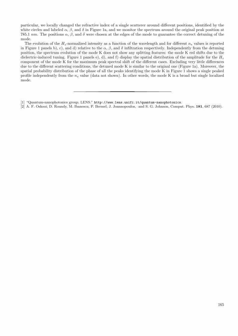
particular, we locally changed the refractive index of a single scatterer around different positions, identified by thewhite circles and labeled α, β, and δ in Figure 1a, and we monitor the spectrum around the original peak position at785.1 nm. The positions α, β, and δ were chosen at the edges of the mode to guarantee the correct detuning of themode.
The evolution of the Hz-normalized intensity as a function of the wavelength and for different ns values is reportedin Figure 1 panels b), c), and d) relative to the α, β, and δ infiltration respectively. Independently from the detuningposition, the spectrum evolution of the mode K does not show any splitting features: the mode K red shifts due to thedielectric-induced tuning. Figure 1 panels e), d), and f) display the spatial distribution of the amplitude for the Hz
component of the mode K for the maximum peak spectral shift of the different cases. Excluding very little differencesdue to the different scattering conditions, the detuned mode K is similar to the original one (Figure 1a). Moreover, thespatial probability distribution of the phase of all the peaks identifying the mode K in Figure 1 shows a single peakedprofile independently from the ns value (data not shown). In other words, the mode K is a broad but single localizedmode.
[1] “Quantum-nanophotonics group, LENS.” http://www.lens.unifi.it/quantum-nanophotonics.[2] A. F. Oskooi, D. Roundy, M. Ibanescu, P. Bermel, J. Joannopoulos, and S. G. Johnson, Comput. Phys. 181, 687 (2010).
165


Acknowledgements
The acknowledgement part is customarily written at the very end during the final rush. Ihope I won’t leave anyone behind.The first thoughts of course go to the members of the Quantum Nanophotonics group
at LENS and my supervisor dott.ssa Costanza Toninelli. I must say I’ve met very fewpeople with the same unlimited drive as yours. Trying to match that positive attitude was amotivating force throughout these years. Thanks for providing support in good and hardertimes, and for granting me the freedom to embark on new projects. During the first twoyears of this PhD I developed a close connection and friendship with Andrea Tabani. Beingolder and more experienced than me, I have always considered him as a reference point.It was thrilling to work with you in the lab, engage in deep discussions and laugh at yourjokes. I always felt like we could read in each other’s minds with a simple glance. In turn,I happened to be a reference person to Sahrish Rizvi, my fellow PhD student. In this case,I was the oldest. I am pleased to have helped you throughout your stay here in Italy. I’velearnt a great deal from your curiosity and spontaneity. It’s been extremely fun to sharethe office with Sofia Pazzagli, who joined our group last year. Always ready to jump intonew adventures, in terms of energy and unbounded scientific interests you are probablythe only one who can match Costanza’s. You definitely managed to make our workplace awarm place. Many thanks to Simona Checcucci, our new and bright PhD student, for yourfriendliness and kindness. The theoretical predictions on the DBT emission pattern shownfor comparison in this thesis are taken from her excellent Master Thesis. Pietro Lombardiand Fabrizio Sgrignuoli, the two post-docs of the group, also deserve a special attention.Though I haven’t worked closely with Pietro, I could in many opportunities appreciate hisvast and sound scientific knowledge. With Fabrizio, a hard-working number cruncher, Ihave worked on the project about the disordered photonic crystals. I admire his spontaneity,sincerity and sociability. During these years, I’ve had the unique and enriching opportunityto meet people from all corners of the world. This is the case for example of the visitingstudents who came to work in our group. Even if he stayed with us for just three months,I quickly became friends with Ankit Rathi, with whom I am pleased to be still in touchafter so many years. Very recently, I had fun speaking French with Eric Laporte. Even morerecently, I am pleased to have met Frederik Dieleman who left just yesterday.
I am grateful to prof. Francesco S. Cataliotti, with whom we shared much more than thelab, for the invaluable support continuously offered to our group. Thanks to the past andpresent members of his group: Cosimo, Stefano, Murtaza, Shahid, Ivan, Florian.

I’d like to give a sincere thank you to Lorenzo Pattelli, a longtime and dear friend withwhom I’ve had the privilege to work very closely. Indeed, the second part of this thesis isthe result of a year and a half of close cooperation. I must say that the amount and depth ofwork that we did wouldn’t have been possible without his intimate knowledge of the subjectand the related literature. Working with you has been inspiring and fun, as we unleashedour creativity through the initial development of MCPlusPlus and the data analysis thatfollowed. It was a pleasure to think aloud and share thoughts with you in the process. Inthe end, it looks like we finally managed to accomplish something together. This is alsoan opportunity to thank his supervisor prof. Diederik Wiersma and all the members of hisgroup: Matteo, Lobre, Sara, Francesco, Dmitry, Simone, Hao, Hua and Camilla. I’ve alwaysenjoyed a very good company with all of them.Several people deserve proper acknowledgement for having provided us access to their
laboratories and equipments. In particular, I thank prof. Massimo Gurioli for sharing theTi:sa laser with us, together with Francesca, Niccolò, Federico, prof.ssa Anna Vinattieriand my fellow LATEX enthusiast Francesco Biccari. Many thanks to prof. Mario Agio forproviding useful insights and always fruitful discussions. With him, I also thank the othermembers of QSTAR, especially Pierfrancesco Buonsante and Filippo Caruso for sharingthe computer cluster with us, which was extensively used for the simulations presented inthis thesis. From INO-CNR, I thank FrancescoMinardi, Alessandro Zavatta for the Ti:salaser and Mario Santoro for the Raman measurements. From CNR, many thanks to BrunoTiribilli for letting us use his Atomic Force Microscope. A special thanks of course goesto all the technicians and staff at LENS, who constantly contribute to the progress of ourresearch.I would like to thank also our collaborators around Europe. In particular, I’m grateful
to prof. Oliver Benson and his Nanooptik group at the Humboldt-Universität zu Berlin,especially Simon Schoenfeld, Günther Kewes, Oliver Neitzke and Jürgen Probst withwhom I’ve had the pleasure to work, even if for a very short time, in Berlin for the AFMmeasurements and for the fabrication of some photonic nanostructures. I also would liketo thank prof. Frank Koppens from ICFO and his group, especially Kevin Schädler andAntoine Reserbat-Plantey, for providing us with the graphene sample and for supportingour work and the related publication.
Last but not least, I would like to thank all my friends and fellow PhD students Lorenzo,Eva, Francesco, Barbara, Davide, Riccardo, Edo and all our common friends. It was apleasure to share this (long) journey with all of you.
I sincerely wish to acknowledge the continuous financial support from project MALICIA –Light-Matter interfaces in absence of cavities (Seventh Framework Programme for Researchof the European Comission, under FET-Open Grant Agreement n. 265522-FP7-ICT-2009-C);the European Laboratory for Non-Linear Spectroscopy (LENS); project GRANCASSA fromthe Ente Cassa di Risparmio di Firenze and project Atom-Based Nanotechnology fromMIUR(progetto premiale CNR-INO).