Single Mode Fiber VP i
16
Photonic Modules > Fibers > FiberNLS FiberNLS Nonlinear Dispersive Fiber (NLS) Purpose When used with sampled-mode signals, this module solves the nonlinear Schroedinger (NLS) equation describing the propagation of linearly-polarized optical waves in fibers using the split-step Fourier method. Depending on the signal representation, different effects are represented: if the signals are in a Single Frequency Band (SFB), or JoinSampledBands = ON, the model takes into account stimulated Raman scattering (SRS), four-wave mixing (FWM), self-phase modulation (SPM), cross-phase modulation (XPM), first order group-velocity dispersion (GVD), second order GVD and attenuation of the fiber. If the signals are in a Multiple Frequency Band (MFB), the above effects are calculated within each band. Use the module UniversalFiber (or UniversalFiberFwd) to include interactions between MFBs and also between MFBs and Parameterized Signals. For Parameterized Signals (CW representation) an ordinary differential equation system including Stimulated Raman Scattering (SRS) and frequency dependent attenuation is applied. For this to operate ConvertToParameterized must be set to ON. Keywords Fiber, Nonlinear, Split Step, Raman, XPM, FWM, SPM, GVD Inputs Outputs Parameters In this section: Physical Numerical\Split-Step Parameters Numerical\Raman Parameters Enhanced Port Purpose Signal/Data Type input Input optical signal Optical Blocks Port Purpose Signal/Data Type output Output optical signal Optical Blocks Seite 1 von 16 FiberNLS 04.02.2014 mk:@MSITStore:C:\Program%20Files\VPI\VPItransmissionMaker%209.1\doc\modu...
-
Upload
mvictoriarg -
Category
Documents
-
view
25 -
download
1
Transcript of Single Mode Fiber VP i

Photonic Modules > Fibers > FiberNLS
FiberNLS
Nonlinear Dispersive Fiber (NLS)
Purpose
When used with sampled-mode signals, this module solves the nonlinear Schroedinger (NLS)
equation describing the propagation of linearly-polarized optical waves in fibers using the split-step
Fourier method. Depending on the signal representation, different effects are represented: if the
signals are in a Single Frequency Band (SFB), or JoinSampledBands = ON, the model takes into
account stimulated Raman scattering (SRS), four-wave mixing (FWM), self-phase modulation
(SPM), cross-phase modulation (XPM), first order group-velocity dispersion (GVD), second order
GVD and attenuation of the fiber. If the signals are in a Multiple Frequency Band (MFB), the above effects are calculated within each band. Use the module UniversalFiber (or UniversalFiberFwd) to
include interactions between MFBs and also between MFBs and Parameterized Signals. For
Parameterized Signals (CW representation) an ordinary differential equation system including Stimulated Raman Scattering (SRS) and frequency dependent attenuation is applied. For this to
operate ConvertToParameterized must be set to ON.
Keywords
Fiber, Nonlinear, Split Step, Raman, XPM, FWM, SPM, GVD
Inputs
Outputs
Parameters
In this section:
PhysicalNumerical\Split-Step ParametersNumerical\Raman Parameters
Enhanced
Port Purpose Signal/Data Type
input Input optical signal Optical Blocks
Port Purpose Signal/Data Type
output Output optical signal Optical Blocks
Seite 1 von 16FiberNLS
04.02.2014mk:@MSITStore:C:\Program%20Files\VPI\VPItransmissionMaker%209.1\doc\modu...

PhysicalPhysicalPhysicalPhysical
Numerical\SplitNumerical\SplitNumerical\SplitNumerical\Split----Step ParametersStep ParametersStep ParametersStep Parameters
Name and Description Unit Type Volatile Value RangeDefault Value
ReferenceFrequency
Reference frequency for the specifiedparameters.
Hz float yes]0;∞[
a 193.1e12
Length
Fiber length.
m float yes[0.0;∞[
a 1.0e3
GroupRefractiveIndex
Group refractive index of thefundamental fiber mode at the reference frequency.
- float yes[0.0;∞[
a 1.47
Attenuation
Fiber attenuation per meter ifAttFileName is not specified.
dB/m float yes[0.0;10e-2]
w 0.2e-3
AttFileName
File for attenuation vs. frequency.
- inputfile yes - -
Dispersion
Dispersion coefficient in terms ofwavelength.
s/m^2 float yes [-500e-6;500e-
6]w
16e-6
DispersionSlope
Slope of the dispersion coefficient with
wavelength.
s/m^3 float yes [-50.0e3;50.0e3]
w
0.08e3
NonLinearIndex
Nonlinear refractive index measuredwith constant linear polarization. For fibers with randomly varying
birefringence this value should be reduced by a factor of 8/9.
m^2/W float yes [-50e-20;50e-
20]a
2.6e-20
CoreArea
Effective core area of the fiber for
nonlinear calculations.
m^2 float yes]0.0;∞[
a 80.0e-12
Tau1
Inverse of the negative frequencyoffset of the Raman gain peak from the Raman pump frequency.
s float yes [1e-15;50e-15]a
12.2e-15
Tau2
1/[2*pi*(width of the Raman gaincurve)].
s float yes [1e-15;50e-15]a
32.0e-15
RamanCoefficient
Fractional contribution of the delayedRaman response.
- float yes[0.0;1.0]
a 0.0
Name and Description Unit Type Volatile Value Range Default Value
StepSelectionMethod
Defines the method for selecting the size of the step in the split-step fourier method. WhenLocalErrorMethod is
selected, the step size is
- enum yes LocalErrorMethod,
NonlinearPhaseChange,ConstantStep
NonlinearPhaseChange
Seite 2 von 16FiberNLS
04.02.2014mk:@MSITStore:C:\Program%20Files\VPI\VPItransmissionMaker%209.1\doc\modu...

governed by
TargetLocalError parameter. If NonlinearPhaseChange is selected, the step size is specified by
MaxPhaseChange parameter. For ConstantStep setting,the fixed step size equal to MaxStepWidth in used in simulation.
SymmetricSplitStep
Type of the split-step Fourier method.(context sensitive)
- enum yes NO, YES No
MaxStepWidth
Maximum step width allowed in the split-step Fourier method.
m float yes]0.0;∞[
a 1.0e3
MinSplitStepWidth
The minimum allowed step width in the split-step Fourier method.(context sensitive)
m float yes[0.0;∞[
a 1.0
InitialSplitStepWidth
Initial step width for local error method in the split-step Fourier algorithm.
(context sensitive)
m float yes]0.0;∞[
a 1.0e3
TargetLocalError
Maximum tolerable local error in the split-step Fourier method. The
step width is chosen in such a way that the local error on a single simulation step is within [TargetLocalError/2;
2*TargetLocalError]. Smaller values of TargetLocalError result in smaller steps, which provide better accuracy, but require longer
computation time. The upper and lower limits of the step width are set by the parametersMaxStepWidth and
MinSplitStepWidth, respectively.(context sensitive)
- float yes]0;∞[
a 1.0e-3
MaxPhaseChange
Maximum tolerable
phase change acrossone step of the split-step Fourier method. The step width is chosen in such a way that the
phase of the optical field in the nonlinear step does not change by more than MaxPhaseChange over
deg float yes]0;∞[
a 0.05
Seite 3 von 16FiberNLS
04.02.2014mk:@MSITStore:C:\Program%20Files\VPI\VPItransmissionMaker%209.1\doc\modu...
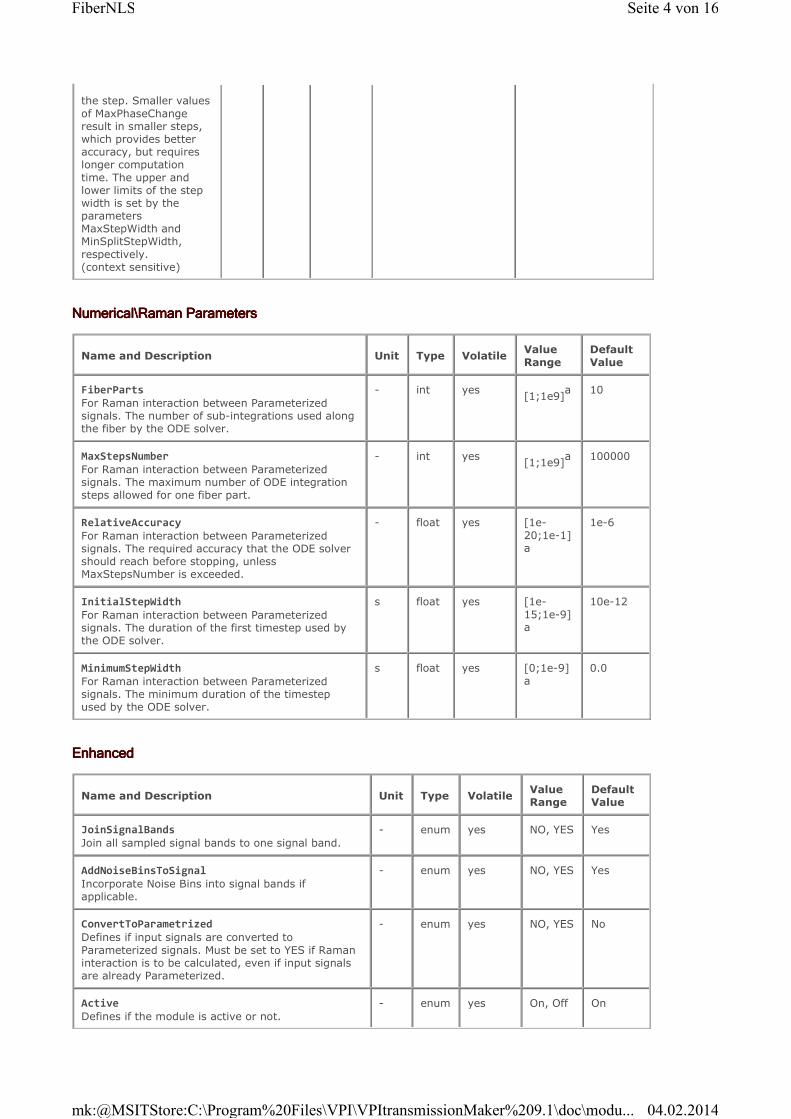
Numerical\Raman ParametersNumerical\Raman ParametersNumerical\Raman ParametersNumerical\Raman Parameters
EnhancedEnhancedEnhancedEnhanced
the step. Smaller values
of MaxPhaseChange result in smaller steps, which provides better accuracy, but requires longer computation
time. The upper and lower limits of the step width is set by the parameters MaxStepWidth and MinSplitStepWidth,
respectively.(context sensitive)
Name and Description Unit Type VolatileValue
Range
Default
Value
FiberParts
For Raman interaction between Parameterized signals. The number of sub-integrations used along the fiber by the ODE solver.
- int yes[1;1e9]
a 10
MaxStepsNumber
For Raman interaction between Parameterized signals. The maximum number of ODE integration steps allowed for one fiber part.
- int yes[1;1e9]
a 100000
RelativeAccuracy
For Raman interaction between Parameterized signals. The required accuracy that the ODE solvershould reach before stopping, unless MaxStepsNumber is exceeded.
- float yes [1e-
20;1e-1]a
1e-6
InitialStepWidth
For Raman interaction between Parameterized signals. The duration of the first timestep used by the ODE solver.
s float yes [1e-
15;1e-9]a
10e-12
MinimumStepWidth
For Raman interaction between Parameterized signals. The minimum duration of the timestep used by the ODE solver.
s float yes [0;1e-9]
a
0.0
Name and Description Unit Type VolatileValue Range
Default Value
JoinSignalBands
Join all sampled signal bands to one signal band.
- enum yes NO, YES Yes
AddNoiseBinsToSignal
Incorporate Noise Bins into signal bands if applicable.
- enum yes NO, YES Yes
ConvertToParametrized
Defines if input signals are converted to
Parameterized signals. Must be set to YES if Raman interaction is to be calculated, even if input signals are already Parameterized.
- enum yes NO, YES No
Active
Defines if the module is active or not.
- enum yes On, Off On
Seite 4 von 16FiberNLS
04.02.2014mk:@MSITStore:C:\Program%20Files\VPI\VPItransmissionMaker%209.1\doc\modu...

Description
The sampled bands must contain a single signal polarization. However, unpolarized noise can be
propagated in Noise Bins. This is useful for saturating optical amplifiers with both polarizations of
noise. However, this unpolarized noise should not be added to the sampled band, as only a linear-
polarization sampled signal can be handled. This requires the Global Parameter InbandNoiseBins =
ON, and the fiber parameter AddNoiseBinsToSignal = OFF.
This is one of the simplest fiber models in the range. It is the basis of many fiber simulations. However, more complex fiber models are provided to offer more flexibility in terms of input data
format, interactions between signal representations, bidirectional Raman amplification, dispersion
decreasing fiber (UniversalFiber or UniversalFiberFwd), polarization mode dispersion
(FiberNLS_PMD), fast simulation of jitter in RZ systems (JitterLongHaul, JitterShortHaul), and
simulation with aperiodic waveforms (TimeDomainFiber).
Note: For simulations where the nonlinear effects are unimportant, simply set NonLinearIndex
to zero and ignore the parameters CoreArea, Tau1, Tau2, RamanCoefficient, and all settings in
the Numerical Parameters category.
The simulation speed of this module can be improved using parallel computations on a multi-core central processing unit (CPU) or a supported graphical processing unit (GPU), see Chapter 3, “User
Interface Reference” in the VPItransmissionMaker™/ VPIcomponentMaker™ User Interface Reference for details on supported hardware and GUI controls for parallel simulations.
The FiberNLS module can use parallel computations for the split-step Fourier algorithm. Both FFT
calculation and multiplication of the sample arrays will be done in parallel.
When both multithreading within modules and GPU-assisted computation are switched on and
supported by the hardware, the module will use the GPU, as it usually reduces the simulation time.
Note: Only calculations with sampled bands will be parallelized, both on the CPU and GPU.
Split-Step Fourier Implementation
In this section:
Dispersion OperatorNonlinear Operator (with no Raman effect)Split-Step Fourier Method
Nonlinear Operator (with Raman effect)
The generalized nonlinear Schrödinger equation is used to describe the inband effects:
where denotes the slowly-varying complex-envelope of the electric field of the light wave,
characterizes its power, is the nonlinearity operator, and is the dispersion
operator.
Dispersion Operator
(1)
Seite 5 von 16FiberNLS
04.02.2014mk:@MSITStore:C:\Program%20Files\VPI\VPItransmissionMaker%209.1\doc\modu...

Note: For linear fibers, this is the only part of the theory that is required, as a single-section model will be applied if the NonLinearIndex is zero.
By removing changing the time reference to remove the intrinsic fiber delay, the dispersion
operator can be written as:
where:
The dispersion parameter, Dλ, has to be entered in SI units [10
-6 s/m
2= 1 ps/(km · nm)]
The dispersion slope parameter, Sλ, also has to be entered in SI units [10
3 s/m
3= 1 ps/
(km · nm2)]
Note: Setting the DispersionSlope to zero does not give a constant pulse spreading on each
WDM channel. This is because the dispersion is specified in terms of wavelength, but
implemented in terms of optical frequency. This is apparent when Dispersion and
DispersionSlope are set to zero, but there remains some pulse spreading.
The parameter AttFileName can be used to specify a file that contains the Attenuation
parameter [dB/m] vs. the optical frequency [Hz]. The file format is:193e12 0.2e3
193.1e12 0.2e3
193.2e12 0.2e3
Nonlinear Operator (with no Raman effect)
If stimulated Raman is to be excluded from the simulation (parameter RamanCoefficient = 0) the
nonlinear operator is simply given by:
(2)
β2 [s
2/m] describes the first order group-velocity dispersion (GVD), and is related to the
Dispersion parameter at the reference wavelength (= c/ReferenceFrequency) by
(3)
β3 [s
3/m] the second order GVD slope, and is related to the DispersionSlope S
λ= dD
λ/dλ by:
(4)
α [1/m] the attenuation constant. The Attenuation parameter a [dB/m] is related to α by
. (5)
(6)
Seite 6 von 16FiberNLS
04.02.2014mk:@MSITStore:C:\Program%20Files\VPI\VPItransmissionMaker%209.1\doc\modu...

and depends on the nonlinear index n2 (parameter NonlinearIndex, see Polarization
Considerations), the effective CoreArea Aeff
, as well as on the reference frequency fref
and the
velocity of light in vacuum c.
Split-Step Fourier Method
The split-step Fourier method divides the fiber into alternate sections of two types. The first type
represents the dispersion in the frequency domain, the second represents the nonlinearity in the
time domain. The choice of step-size is crucial in achieving a balance between computation time
and accuracy.
The step size, Δz (the length of fiber represented by one nonlinearity and one dispersion operator)
is determined according to the following parameter settings:
When using the local error method, the following should be observed:
where Δφnl
(radians) is the maximum acceptable nonlinear phase shift1. The parameter
MaxPhaseChange sets the maximum acceptable phase change (but in degrees) and is normally
within the range of 0.06…0.2 degs.
Note: For both local error and nonlinear phase change methods, the step size is limited from
above and below by settings of the parameters MaxStepWidth and MinSplitStepWidth,
respectively.
If the desired step size is less than MinSplitStepWidth, the module will stop with an error
message. Normally, the minimal step size should be set as a ‘guard condition’ to ensure that the simulation will not take an excessive amount of time.
If the desired step size is larger than MaxStepWidth, the module will use the maximal allowed
step size. This is normally set to be far less than the walk-off length (the fiber distance that
produces a relative phase shift of 2π radians between the carriers) between two optical carriers due to dispersion. Obviously, the wider the WDM spectrum within a SFB, the shorter
the step length should be. This actually shows that it is better to model a few WDM channels
in an SFB, than all channels (this is called the Mean Field Approach, and is discussed in the VPItransmissionMaker™Optical Systems User’s Manual).
If StepSelectionMethod = LocalErrorMethod, the module takes the step according to the
algorithm described in [1], maintaining the relative error at each step within range [ε/2; ε],
where the desired error value ε is defined by the parameter TargetErrorValue. This mode is
rather similar to adaptive step algorithms routinely used in ordinary differential equations.
+ Local error method has greater order with respect to step size than the other optionsavailable for the fiber modules, which means that it will be more efficient (require less steps) for high-accuracy simulations. However, due to a larger number of computations per
step, low-accuracy simulations can be somewhat longer.
+ In some cases, such as propagation of several frequency components in a shifted-
dispersion fiber, local error method tends to make larger errors in low-power regions of the
spectrum (like the FWM products).
If StepSelectionMethod = NonlinearPhaseChange, the step size, Δzφ
, determined by not
allowing the nonlinear phase shift (proportional to optical power) to exceed a defined value,
MaxPhaseChange. This gives a step size
(7)
Seite 7 von 16FiberNLS
04.02.2014mk:@MSITStore:C:\Program%20Files\VPI\VPItransmissionMaker%209.1\doc\modu...

Assuming a propagation of optical signals in +z direction and a symmetrical split-step algorithm
(parameter SymmetricSplitStep is set to YES, or if the parameter StepSelectionMethod is set to
LocalErrorMethod2), the mathematical formalism of the procedure can be described as follows:
If the parameter SymmetricSplitStep is set to NO, the equation changes to:
The nonlinearity operator is applied on the field at locus z0. Therefore, the exact dependence of
operator on the time-dependent amplitude in the interval Δz is replaced by its start value:
Nonlinear Operator (with Raman effect)
If the parameter RamanCoefficient is not zero, the nonlinearity operator is extended to:
where (parameter RamanCoefficient) represents the fractional contribution of the delayed
Raman response which is approximated by:
In Equation 11, (parameter Tau1) and (parameter Tau2) are two adjustable parameters to
provide a good fit to the Raman-gain spectrum:
The commonly used values are =0.18, τ1=12.2 fs, τ
2=32 fs giving an offset of 13 THz and a
width of 10 THz. The approximated Raman gain and a realistic spectrum which has been measured in silica fibers are shown in Figure 1.
If StepSelectionMethod = ConstantStep, the constant step size equal to the value of the
MaxStepWidth parameter will be used.
(8)
(9)
(10)
(11)
, t > 0 (12)
Tau1 (s) is the inverse of the frequency offset (in radians/s) between the Raman pump and
peak Raman gain,
Seite 8 von 16FiberNLS
04.02.2014mk:@MSITStore:C:\Program%20Files\VPI\VPItransmissionMaker%209.1\doc\modu...

Figure 1 Example of the measured (thick line) and approximated (thin line, default parameter setting) Raman spectra for pure silica at 1500 nm
Parameterized Signals and Noise Bins: Raman scattering
In this section:
Polarization Considerations
For Parameterized Signals and Noise Bins, the effect of stimulated Raman scattering is modeled by
the following ordinary differential equations:
where Aiis the amplitude of the i th Parameterized Signal, N
k is the amplitude of the k th Noise Bin,
and αi, α
kare representing their attenuation coefficients, respectively. In Equation 12, f
rdescribes
(13)
the fractional contribution of the delayed Raman response to the nonlinearity coefficient γ, and
represents the imaginary part of the Fourier-transformed Raman response function
at the frequency difference between the Parameterized Signals (fi− f
m). In the lower equation,
denotes the imaginary part of the Fourier transformed Raman response function at
the frequency difference between the Noise Bins and the Parameterized Signals.
This system of ordinary differential equations is solved using a 4th-order Runge-Kutta equation
solver. The parameters MaxStepsNumber, MaxPhaseChange, RelativeAccuracy, InitialStepWidth,
MinimumStepwidth are used to tune the equation solver. The parameter FiberParts can be used to
subdivide the fiber length into several sections. For each of these parts the integration algorithm is
restarted.
The demonstration Optical Systems Demos > Characterization > Raman Scattering > Raman Power Transfer illustrates this mode of operation.
Polarization Considerations
Seite 9 von 16FiberNLS
04.02.2014mk:@MSITStore:C:\Program%20Files\VPI\VPItransmissionMaker%209.1\doc\modu...

SPM is different for linear, circular and random polarizations. In a real fiber, Polarization-Mode
Dispersion (PMD) leads to a random evolution of polarization (between linear and circular) along the
fiber, which means that the strength of the SPM varies along the fiber (linear polarization produces
a stronger peak field than circular polarization). Averaging over all polarization states (assuming
complete polarization mixing, i.e., when the fiber is much longer than the beat length and
correlation length) gives a well-known factor of 8/9. This factor is often already included in the
measured value of the nonlinear refractive index, n2. In this case, the n
2 value can be directly used
for the parameter NonlinearIndex. However, if you use the n2 value that has been measured
without this correction, i.e. for constant linear polarization, the measured n2
should be multiplied by
a factor 8/9 before being input as a parameter.
To model the average effect of XPM between channels (using a SFB), where the polarizations of the
channels rotate with respect to one another over the length of the fiber, the nonlinear factor should
be reduced by a factor 2/3 (or 3/4 if the measured n2 value already includes the 8/9 factor). For
worst-case calculations (where the polarization remains linear along the fiber), the nonlinear
refractive index should not be reduced. Note that it is not possible to apply valid correction factors
simultaneously to SPM and XPM using this model. For accurate simultaneous simulation of the
mentioned effects the more complex fiber models FiberNLS_PMD, UniversalFiber or
UniversalFiberFwd should be used.
Signal Representation
In this section:
Block
Block
Single Frequency Bands (SFBs) are simulated using the split-step Fourier method. All signals are assumed to be polarization aligned within the band.
Multiple Frequency Bands (MFBs) are individually simulated using the split-step Fourier method. No
interaction between the bands is calculated. That is, Raman power transfer, XPM and FWM between
the bands are not calculated. MFBs may be converted to an SFB by setting JoinSignalBands to ON.
Parameterized Signals are computed solving the above system of ordinary differential equations
using a 4th-order Runge-Kutta equation solver. ConvertToParameterized should be set to ON. Any
sampled signals will be converted to Parameterized Signals if ConvertToParameterized is set to ON.
For parameterized signals, the values of a number of physical parameters are saved to the tracking
data (see Chapter 5 of the VPItransmissionMaker™Optical Systems User’s Manual). They can be
visualized using the LinkAnalyzer module. The fiber parameter GroupRefractiveIndex is used to
calculate the fiber delay (TransitTime in LinkAnalyzer).
The accumulated self-phase modulation in the signal tracking data is characterized by the phase
shift and is calculated according to [2]
where is the input signal power and is the effective fiber length.
Noise Bins
The system of ordinary differential equations includes the interaction between Noise Bins and
Parameterized Signals when ConvertToParameterized is set to ON.
Boundary Conditions
Periodic. For Aperiodic Boundary Conditions see TimeDomainFiber.
(14)
Seite 10 von 16FiberNLS
04.02.2014mk:@MSITStore:C:\Program%20Files\VPI\VPItransmissionMaker%209.1\doc\modu...

Reinitialization Behavior
Multiple Runs
Reinitialization is performed after each run.
Restart of Simulation or Reset during Simulation
Reinitialization is performed.
Reset during Simulation
Reinitialization is performed.
Module Deactivation
If parameter Active is OFF, the optical input signals will be passed through the module without any
changes.
Validation
In this section:
(1) Spectral broadening of a Gaussian pulse due to Self-Phase Modulation (SPM)(2) Temporal evolution of solitons
i) Fundamental solitonii) Second order Soliton
This section is intended to prove the agreement of known theoretical predictions for optical fibers.
Since there are numerous theoretical aspects to compare with the behavior of computational
applications, a choice of two test runs has been made focusing on both the nonlinear and dispersive
properties implemented in the module.
The two test runs explained below concentrate on the temporal and/or spectral evolution of single
pulses in single channels.
(1) Spectral broadening of a Gaussian pulse due to Self-Phase Modulation (SPM)
a) Theory
It is known [2], that in the limit of (no GVD) the nonlinear Schrödinger equation
becomes
where the normalized amplitude U (z,τ) is related to the field amplitude A(z,τ) by
The nonlinear length LNL
is introduced by
where γ is defined as described above and P0 is the peak power of the Gaussian pulse. The solution
(15)
(16)
(17)
Seite 11 von 16FiberNLS
04.02.2014mk:@MSITStore:C:\Program%20Files\VPI\VPItransmissionMaker%209.1\doc\modu...

to (15) is given by
with a phase argument
The effective fiber length zeff
becomes zeff
= z if α = 0 (no fiber loss) is assumed. The phase shift is
time-dependent and gives rise to a frequency chirp δ ω(t). The latter is given for a Gaussian pulse
by
where is the spectral width of the initial pulse, and Φmax
is the maximum phase shift
which is reached at the pulse center [2]. The spectral broadening is thus a function of the pulse
power and the propagation length z.
b) Simulation
TThe most important parameters are: PeakPower, NonlinearIndex, Length.
After every fiber length , the maximum phase shift is increased by one radian which, in
turn, gives rise to an interference pattern stemming from the superposition of the chirped pulse’s
frequency components. The number of peaks in the spectrum of the pulse M is approximately given by the relation
c) Results
The simulation has been performed with fiber lengths giving 0 π, 0.5 π, …, 3.5 π maximum phase
shift. The spectral plots resulting from this simulation are shown in Figure 2 and are in good
agreement with [2].
(18)
(19)
(20)
Seite 12 von 16FiberNLS
04.02.2014mk:@MSITStore:C:\Program%20Files\VPI\VPItransmissionMaker%209.1\doc\modu...

Figure 2 Spectrum of a Gaussian pulse as it propagates along the Fiber (Simulation Results). Parameters used: SampleRate 1024e9, BitRate 1e9, Bits 1, FWHM 1/(16*BitRate), PeakPower 0.1,
PRBSType ONE.
(2) Temporal evolution of solitons
Solitons are of major interest in optical fiber communications. The term “soliton” refers to special
kinds of waves that can propagate undistorted over long distances and remain unaffected after
collision with each other. Ideal Solitons exist in fibers with anomalous group-velocity dispersion (D
> 0, β2< 0, cf. (4)) and vanishing loss. Solitons are well suited for functional tests of this module,
since both nonlinear and dispersive properties enter into the numerical simulation.
i) Fundamental soliton
a) Theory
The analytic solution representing solitons is obtained, e.g., applying the inverse scattering method [2] [p. 142] to the nonlinear Schrödinger equation. This method leads to a general solution for
solitons of different orders. The fundamental soliton (first order) will propagate undistorted without
change in shape for arbitrarily long distances. A higher-order soliton exhibits an oscillating pattern of its temporal and spectral evolution.These spatial variations are periodic with length of z
0 (soliton
period) for solitons with an integer order.
A fundamental soliton is given by the analytic expression
with the normalized field amplitude U (ξ, τ), cf. (16), and
(22)
Seite 13 von 16FiberNLS
04.02.2014mk:@MSITStore:C:\Program%20Files\VPI\VPItransmissionMaker%209.1\doc\modu...
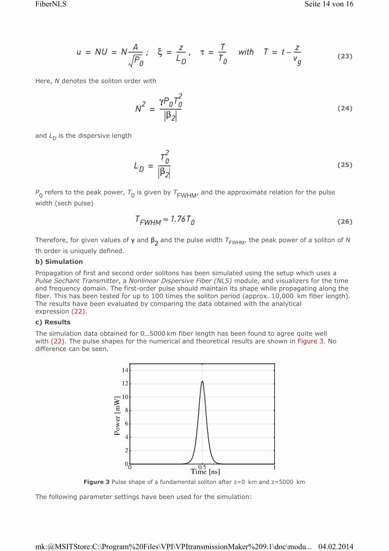
Here, N denotes the soliton order with
and LD is the dispersive length
P0 refers to the peak power, T
0 is given by T
FWHM, and the approximate relation for the pulse
width (sech pulse)
Therefore, for given values of γ and β2 and the pulse width T
FWHM, the peak power of a soliton of N
th order is uniquely defined.
b) Simulation
Propagation of first and second order solitons has been simulated using the setup which uses a
Pulse Sechant Transmitter, a Nonlinear Dispersive Fiber (NLS) module, and visualizers for the time and frequency domain. The first-order pulse should maintain its shape while propagating along the
fiber. This has been tested for up to 100 times the soliton period (approx. 10,000 km fiber length).
The results have been evaluated by comparing the data obtained with the analytical
expression (22).
c) Results
The simulation data obtained for 0…5000 km fiber length has been found to agree quite well
with (22). The pulse shapes for the numerical and theoretical results are shown in Figure 3. No
difference can be seen.
Figure 3 Pulse shape of a fundamental soliton after z=0 km and z=5000 km
The following parameter settings have been used for the simulation:
(23)
(24)
(25)
(26)
Seite 14 von 16FiberNLS
04.02.2014mk:@MSITStore:C:\Program%20Files\VPI\VPItransmissionMaker%209.1\doc\modu...
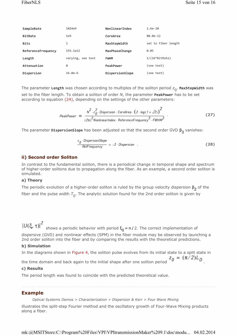
The parameter Length was chosen according to multiples of the soliton period z0. MaxStepWidth was
set to the fiber length. To obtain a soliton of order N, the parameter PeakPower has to be set
according to equation (24), depending on the settings of the other parameters:
The parameter DispersionSlope has been adjusted so that the second order GVD β3 vanishes:
ii) Second order Soliton
In contrast to the fundamental soliton, there is a periodical change in temporal shape and spectrum
of higher-order solitons due to propagation along the fiber. As an example, a second order soliton is simulated.
a) Theory
The periodic evolution of a higher-order soliton is ruled by the group velocity dispersion β2 of the
fiber and the pulse width T0. The analytic solution found for the 2nd order soliton is given by
shows a periodic behavior with period ξ0
= π / 2. The correct implementation of
dispersive (GVD) and nonlinear effects (SPM) in the fiber module may be observed by launching a
2nd order soliton into the fiber and by comparing the results with the theoretical predictions.
b) Simulation
In the diagrams shown in Figure 4, the soliton pulse evolves from its initial state to a split state in
the time domain and back again to the initial shape after one soliton period .
c) Results
The period length was found to coincide with the predicted theoretical value.
Example
Optical Systems Demos > Characterization > Dispersion & Kerr > Four Wave Mixing
illustrates the split-step Fourier method and the oscillatory growth of Four-Wave Mixing products along a fiber.
SampleRate 1024e9 NonlinearIndex 2.6e20
BitRate 1e9 CoreArea 80.0e12
Bits 1 MaxStepWidth set to fiber length
ReferenceFrequency 193.1e12 MaxPhaseChange 0.05
Length varying, see text FWHM 1/(16*BitRate)
Attenuation 0 PeakPower (see text)
Dispersion 16.0e6 DispersionSlope (see text)
. (27)
. (28)
Seite 15 von 16FiberNLS
04.02.2014mk:@MSITStore:C:\Program%20Files\VPI\VPItransmissionMaker%209.1\doc\modu...

Figure 4 Time evolution of a 2nd order soliton (N = 2). The fiber length is expressed in terms of
the periodic length . Parameter Settings: SampleRate 1024e9, NonlinearIndex 2.6e
20, BitRate 1e9, CoreArea 80.0e12, Bits 1, MaxStepWidth 1.0e3, RefFrequency 193.1e12,
MaxPhaseChange 0.05, Length (see text), FWHM 1/(16*BitRate), Attenuation 0, PeakPower (see
previous text), Dispersion 16.0e6, DispersionSlope (see previous text).
References
Setting to Δφnl
to 2π radians gives the Nonlinear Length, which is a useful metric.
The local error method implicitly uses symmetrical split-step algorithm, see details in [1].
Photonic Modules > Fibers > FiberNLS
[1] O. V. Sinkin, R. Holzlönner, J. Zweck, C.R. Menyuk, “Optimization of the split-step Fourier method in modeling optical-fiber communications systems,” J. Lightwave Technol., vol. 21, no. 1, pp. 61–68,
January 2003.
[2] G.P. Agrawal, Fiber-Optic Communication Systems, 2nd edition. Wiley Interscience, 1997, pp. 62-63.
[3] G. P. Agrawal, Nonlinear Fiber Optics, Academic Press, 1995.
1
2
© 2014 VPIphotonics GmbH
All rights reserved.www.VPIphotonics.com
forums.VPIphotonics.com
Seite 16 von 16FiberNLS
04.02.2014mk:@MSITStore:C:\Program%20Files\VPI\VPItransmissionMaker%209.1\doc\modu...


![Fiber for DUT [Compatibility Mode]](https://static.fdocuments.us/doc/165x107/577d2fd91a28ab4e1eb2dce6/fiber-for-dut-compatibility-mode.jpg)